mahabub-05

7/29/2019 Mahabub-05

http://slidepdf.com/reader/full/mahabub-05 1/9

I.Extensions of the option pricing model:

All the models discussed so far have assumed that the stock price is generated by a

continuous stochastic process with a constant variance. There are two model here for the

extension of the option pricing model, these are

I) Changing the Distributional Assumptions which assume about distribution of stock

prices that changes the model

II) Options to Value Special Situations which consider the various special circumstances

that cause us to consider alternations in the model parameter definitions.

These two extensions are discussed elaborately in the following

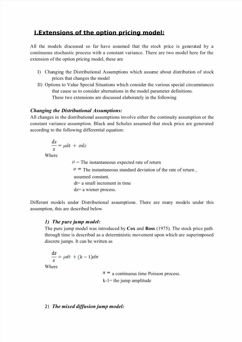
Changing the Distributional Assumptions:

All changes in the distributional assumptions involve either the continuity assumption or the

constant variance assumption. Black and Scholes assumed that stock price are generated

according to the following differential equation:

Where

= The instantaneous expected rate of return

The instantaneous standard deviation of the rate of return ,

assumed constant.

dt= a small increment in time

dz= a wiener process.

Different models under Distributional assumptions. There are many models under this

assumption, this are described below.

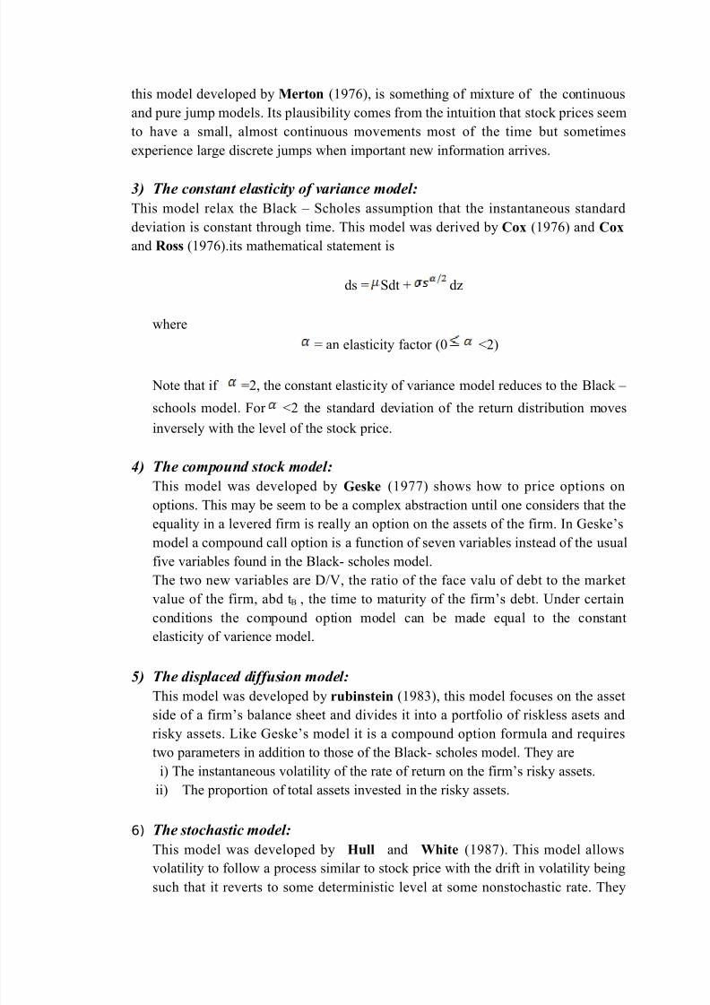
1) The pure jump model:

The pure jump model was introduced by Cox and Ross (1975). The stock price path

through time is described as a deterministic movement upon which are superimposed

discrete jumps. It can be written as

Where

a continuous time Poisson process.

k-1= the jump amplitude

2) The mixed diffusion jump model:

7/29/2019 Mahabub-05


this model developed by Merton (1976), is something of mixture of the continuous

and pure jump models. Its plausibility comes from the intuition that stock prices seem

to have a small, almost continuous movements most of the time but sometimes

experience large discrete jumps when important new information arrives.

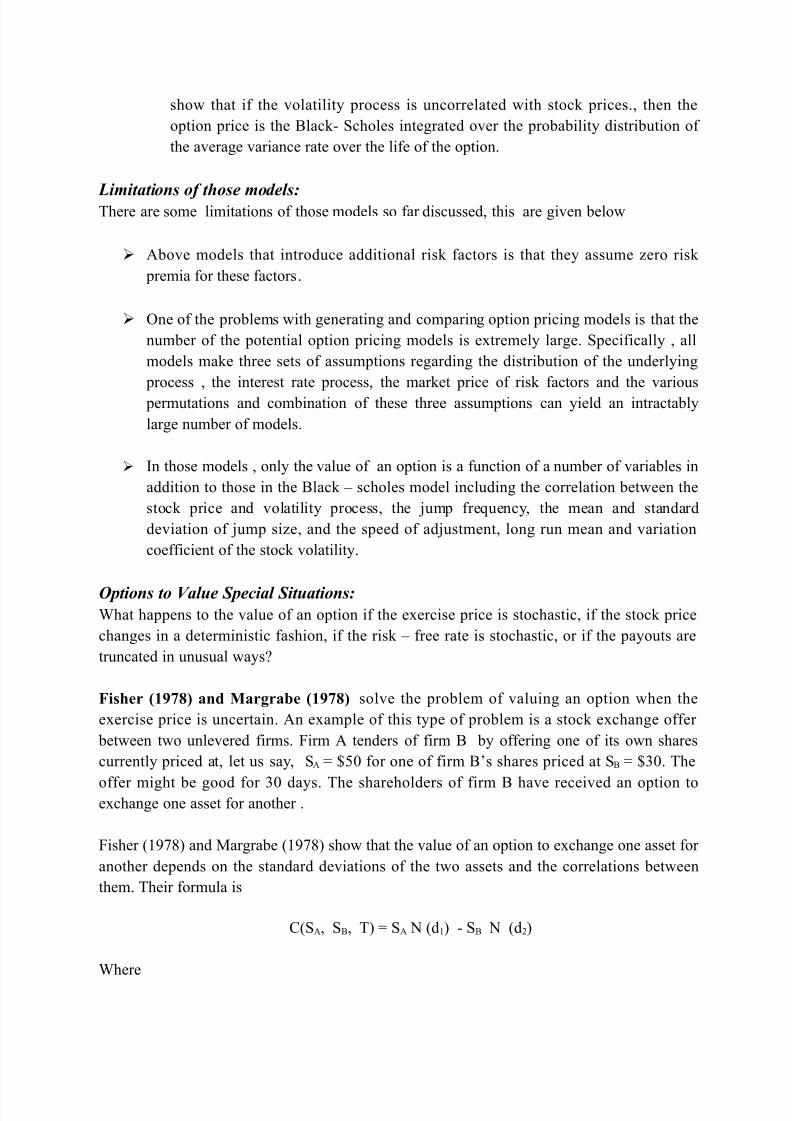
3) The constant elasticity of variance model:

This model relax the Black – Scholes assumption that the instantaneous standard

deviation is constant through time. This model was derived by Cox (1976) and Cox

and Ross (1976).its mathematical statement is

ds = Sdt + dz

where

= an elasticity factor (0 <2)

Note that if =2, the constant elasticity of variance model reduces to the Black –

schools model. For <2 the standard deviation of the return distribution moves

inversely with the level of the stock price.

4) The compound stock model:

This model was developed by Geske (1977) shows how to price options on

options. This may be seem to be a complex abstraction until one considers that the

equality in a levered firm is really an option on the assets of the firm. In Geske’smodel a compound call option is a function of seven variables instead of the usual

five variables found in the Black- scholes model.

The two new variables are D/V, the ratio of the face valu of debt to the market

value of the firm, abd tB , the time to maturity of the firm’s debt. Under certain

conditions the compound option model can be made equal to the constant

elasticity of varience model.

5) The displaced diffusion model:

This model was developed by rubinstein (1983), this model focuses on the asset

side of a firm’s balance sheet and divides it into a portfolio of riskless asets and

risky assets. Like Geske’s model it is a compound option formula and requires

two parameters in addition to those of the Black- scholes model. They are

i) The instantaneous volatility of the rate of return on the firm’s risky assets.

ii) The proportion of total assets invested in the risky assets.

6) The stochastic model:

This model was developed by Hull and White (1987). This model allows

volatility to follow a process similar to stock price with the drift in volatility being

such that it reverts to some deterministic level at some nonstochastic rate. They

7/29/2019 Mahabub-05


show that if the volatility process is uncorrelated with stock prices., then the

option price is the Black- Scholes integrated over the probability distribution of

the average variance rate over the life of the option.

Limitations of those models:There are some limitations of those models so far discussed, this are given below

Above models that introduce additional risk factors is that they assume zero risk

premia for these factors.

One of the problems with generating and comparing option pricing models is that the

number of the potential option pricing models is extremely large. Specifically , all

models make three sets of assumptions regarding the distribution of the underlying

process , the interest rate process, the market price of risk factors and the various

permutations and combination of these three assumptions can yield an intractably

large number of models.

In those models , only the value of an option is a function of a number of variables in

addition to those in the Black – scholes model including the correlation between the

stock price and volatility process, the jump frequency, the mean and standard

deviation of jump size, and the speed of adjustment, long run mean and variation

coefficient of the stock volatility.

Options to Value Special Situations:What happens to the value of an option if the exercise price is stochastic, if the stock price

changes in a deterministic fashion, if the risk – free rate is stochastic, or if the payouts are

truncated in unusual ways?

Fisher (1978) and Margrabe (1978) solve the problem of valuing an option when the

exercise price is uncertain. An example of this type of problem is a stock exchange offer

between two unlevered firms. Firm A tenders of firm B by offering one of its own shares

currently priced at, let us say, SA = $50 for one of firm B’s shares priced at SB = $30. The

offer might be good for 30 days. The shareholders of firm B have received an option toexchange one asset for another .

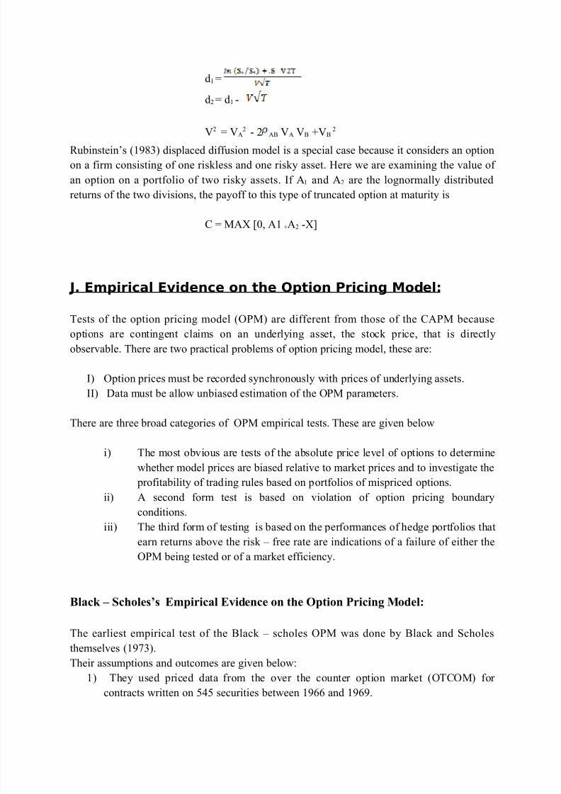
Fisher (1978) and Margrabe (1978) show that the value of an option to exchange one asset for

another depends on the standard deviations of the two assets and the correlations between

them. Their formula is

C(SA, SB, T) = SA N (d1) - SB N (d2)

Where

7/29/2019 Mahabub-05


d1 =

d2 = d1 -

V2 = VA2 - 2 AB VA VB +VB

2

Rubinstein’s (1983) displaced diffusion model is a special case because it considers an option

on a firm consisting of one riskless and one risky asset. Here we are examining the value of

an option on a portfolio of two risky assets. If A1 and A2 are the lognormally distributed

returns of the two divisions, the payoff to this type of truncated option at maturity is

C = MAX [0, A1 +A2 -X]

J. Empirical Evidence on the Option Pricing Model:

Tests of the option pricing model (OPM) are different from those of the CAPM because

options are contingent claims on an underlying asset, the stock price, that is directly

observable. There are two practical problems of option pricing model, these are:

I) Option prices must be recorded synchronously with prices of underlying assets.

II) Data must be allow unbiased estimation of the OPM parameters.

There are three broad categories of OPM empirical tests. These are given below

i) The most obvious are tests of the absolute price level of options to determine

whether model prices are biased relative to market prices and to investigate the

profitability of trading rules based on portfolios of mispriced options.

ii) A second form test is based on violation of option pricing boundary

conditions.

iii) The third form of testing is based on the performances of hedge portfolios that

earn returns above the risk – free rate are indications of a failure of either the

OPM being tested or of a market efficiency.

Black – Scholes’s Empirical Evidence on the Option Pricing Model:

The earliest empirical test of the Black – scholes OPM was done by Black and Scholes

themselves (1973).

Their assumptions and outcomes are given below:

1) They used priced data from the over the counter option market (OTCOM) for

contracts written on 545 securities between 1966 and 1969.

7/29/2019 Mahabub-05


2) Options traded on the OTCOM did not have standardized exercise prices or maturity

dates

3) Whenever the stock went ex- dividend, the exercise price on outstanding options was

lowered by the amount of the dividend.

4) The secondary market in nonstandardized OTCOM option was virtually nonexistent.5) They adopted a test procedure that used the OPM to generate the expected prices of

each option on each trading day.

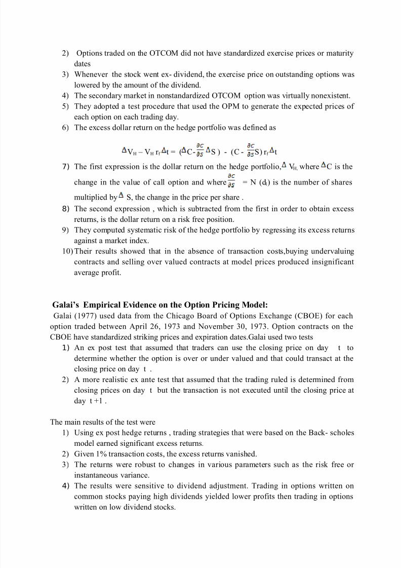
6) The excess dollar return on the hedge portfolio was defined as

VH – VH r f t = ( C- S ) - (C - S) r f t

7) The first expression is the dollar return on the hedge portfolio, VH, where C is the

change in the value of call option and where = N (d1) is the number of shares

multiplied by S, the change in the price per share .8) The second expression , which is subtracted from the first in order to obtain excess

returns, is the dollar return on a risk free position.

9) They computed systematic risk of the hedge portfolio by regressing its excess returns

against a market index.

10) Their results showed that in the absence of transaction costs,buying undervaluing

contracts and selling over valued contracts at model prices produced insignificant

average profit.

Galai’s Empirical Evidence on the Option Pricing Model:

Galai (1977) used data from the Chicago Board of Options Exchange (CBOE) for each

option traded between April 26, 1973 and November 30, 1973. Option contracts on the

CBOE have standardized striking prices and expiration dates.Galai used two tests

1) An ex post test that assumed that traders can use the closing price on day t to

determine whether the option is over or under valued and that could transact at the

closing price on day t .

2) A more realistic ex ante test that assumed that the trading ruled is determined from

closing prices on day t but the transaction is not executed until the closing price at

day t +1 .

The main results of the test were

1) Using ex post hedge returns , trading strategies that were based on the Back- scholes

model earned significant excess returns.

2) Given 1% transaction costs, the excess returns vanished.

3) The returns were robust to changes in various parameters such as the risk free or

instantaneous variance.

4) The results were sensitive to dividend adjustment. Trading in options written on

common stocks paying high dividends yielded lower profits then trading in optionswritten on low dividend stocks.

7/29/2019 Mahabub-05


5) Deviations from the model specifications led to worse performance.

6) Tests of spread strategies yielded results similar to those produced by hedging

strategies described above.

Bhattacharya,s empirical evidence on option pricing model:

He used CBOE transaction data from August 1976 to June 1977. He looked at three different

boundary conditions. An immediate exercise test was composed of situation where the trader

could earn more from exercising immediately from keeping his or her option alive. For a

sample of 86137 there were 1120 immediate exercise opportunities assuming zero transaction

costs. similar results was obtained for test of dividend adjusted lower bound for European call

option and for American call options.

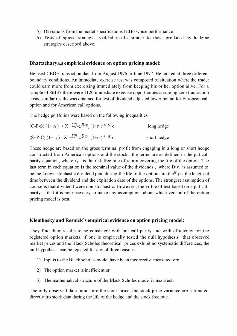
The hedge portfolios were based on the following inequalities

(C-P-S) (1+ r f ) + X + j (1+r f )&j o long hedge

(S+P-C) (1+ r f ) -X + j (1+r f )&j o short hedge

These hedge are based on the gross terminal profit from engaging in a long or short hedge

constructed from American options and the stock . the terms are as defined in the put call

parity equation, where r f is the risk free rate of return covering the life of the option. The

last term in each equation is the teeminal value of the dividends , where Div j is assumed to

be the known stochastic dividend paid during the life of the option and the j is the length of

time between the dividend and the expiration date of the options. The strongest assumption of

course is that dividend were non stochastic. However , the virtue of test based on a put call

parity is that it is not necessary to make any assumptions about which version of the option

pricing model is best.

Klemkosky and Resnick’s empirical evidence on option pricing model:

They find their results to be consistent with put call parity and with efficiency for the

registered option markets. if one is empirically tested the null hypothesis that observed

market prices and the Black Scholes theoretical prices exhibit no systematic differences, the

null hypothesis can be rejected for any of three reasons:

1) Inputs to the Black scholes model have been incorrectly measured orr

2) The option market is inefficient or

3) The mathematical structure of the Black Scholes model is incorrect.

The only observed data inputs are the stock price, the stock price variance are estimated

directly fro stock data during the life of the hedge and the stock free rate.

7/29/2019 Mahabub-05


Using CBOE daily closing prices between December 31, 1975 and December 31,1976 for all

call options listed for six major companies.

MacBeth and Merville empirical evidence on option pricing model:

In their first paper they estimated the implied standard deviation of the rate of return for the

underlying common stock br employing the Black Scholes model. Then by assuming that the

B-S model correctly prices at the money options with at least 90 days to expiration they are

able to estimate the percent deviation of observed call prices from B-S call prices. They

conclude that

1) The Black Scholes model prices are on average less than market prices for in the

money options.

2) The extent to which the Black Scholes model under prices an in the money option and

increases with the extent to which the option is in the money and decreases as the time

to decreases.

3) The Black Scholes model prices of out of the money options with less than 90 days to

expiration are, on the average, greater than market prices, but there does not appear to

be any consistent relationship between the extent to which thes options are overpriced

by the B-S model and the degree to which these options are out of the money or the

time to expiration.

The second Macbeth and merville paper compares the B-S model against the constant

elasticity of variance (CEV) model. The primary differences between two models is that the

B-S model assumes the variance of returns on the underlying assets remains constant,

whereas the constant elasticity of variance model assume the variance changes when the

stock price does.

Others empirical evidences on the option pricing model:

Beckers (1980)also compares the constant elasticity of variance with the B-S model. He uses

1253 daily observation for 47 different stocks to test the B-S assumption that the stock

variance is not a function of the stock price. The data reject this hypothesis.

Geske and Roll (1984) used transactions data for all option traded at middly on August

24,1976. A subsample of 119 options on 28 different stocks with zero schedule dividends

during their remaining life was identified within the main sample. Using regression analysis ,

they demonstrate that the original time, in versus out of the money.

7/29/2019 Mahabub-05


Nonparamatic tests of options paired either by differences in time to maturity or in exercise

prices were performed for two time periods.

1) August 21,1976 to October 21,1977

2) October 24,1977 to August 31,1978

Two interesting conclusions were found. First if the time to maturity is held constant , then he

B-S model is biased, but the direction of the bias is different in the two time periods that were

investigated. The second conclusion was that although some of the alternative pricing models

were compatible with the empirical results, none of them were superior in both time periods.

Amin and Ng (1993) test the ability of autoregressive conditionally heteroscedastic. They

find that the ARCH models display both moneyness and maturity related biases. On the other

hand they also find in terms of pricing errors that the model performed

Summary:Closed form solutions to the option pricing problem have been developed relatively

recently. Yet their potential for applications to problems in finance is tremendous. Almost all

financial assets are really contingent claim. Fro example, common stock is really a call option

on the value of the assets of levered firm. Similarly, risky debt, insurance, warrens and

convertible debt may all be thought of as options. Also, options pricing theory implications

for the capital structures of the firm, for investment policy, for merger and acquisitions, for

spin offs and for dividend policy. State preference theory, the capital assets pricing model,

arbitrage pricing theory and option pricing are disused here.

We have established that option pricing are functions of five parameters, the price of the

underlying security, its instantaneous variance, the exercise price on the option, the time to

maturity and the risk free rate. only one of these variables, the instantaneous variance is not

directly observables. Even more interesting is the fact that the option price does not depend:

I. On individual risk preferences or

II. On the expected rate of return on the underlying assets.

Both result follow from the fact that option prices are determined from pure arbitrageconditions available to the investors who established perfectly hedge portfolios.

Much remains to be done to empirically test the validity of the options pricing model in

general and of various versions of it such as the Black – scholea model, and other models that

incorporate additional risk factors. The empirical results thus far tend to be mixed. A number

of papers have reported the more complex models do not do significantly better than the

simple Black Scholes option pricing model. On the other hand, statistically significant

departures from the Black Scholes model have discovered, with indications that that the

departures are consistent with the market pricing additional risk such as stochastic volatility

and random jumps.

7/29/2019 Mahabub-05


mahabub-05

Documents