HAL Id: hal-00863802https://hal-brgm.archives-ouvertes.fr/hal-00863802

Submitted on 19 Sep 2013

HAL is a multi-disciplinary open accessarchive for the deposit and dissemination of sci-entific research documents, whether they are pub-lished or not. The documents may come fromteaching and research institutions in France orabroad, or from public or private research centers.

L’archive ouverte pluridisciplinaire HAL, estdestinée au dépôt et à la diffusion de documentsscientifiques de niveau recherche, publiés ou non,émanant des établissements d’enseignement et derecherche français ou étrangers, des laboratoirespublics ou privés.

Magnitude scaling of induced earthquakesBenjamin Edwards, John Douglas

To cite this version:Benjamin Edwards, John Douglas. Magnitude scaling of induced earthquakes. Geothermics, Elsevier,2014, 52, pp.132-139. <10.1016/j.geothermics.2013.09.012>. <hal-00863802>

1

Magnitude Scaling of Induced Earthquakes

Benjamin Edwards 1* and John Douglas 2

1 Swiss Seismological Service, ETH Zürich, Zürich, Switzerland.

2 Seismic and Volcanic Risks Unit (RSV), Risks and Prevention Division (DRP), BRGM, Orléans, France.

* Corresponding Author -- email: edwards@sed.ethz.ch; address: Swiss Seismological Service, ETH

Zürich, Sonneggstrasse 5, 8092 Zürich, Switzerland; telephone: +41 44 632 8963.

Abstract

Presented are the results of an earthquake magnitude homogenization exercise for several datasets

of induced earthquakes. The result of this exercise is to show that homogeneous computation of

earthquake moment- and local-magnitude is useful in hazard assessment of Enhanced Geothermal

Systems (EGSs). Data include records from EGSs in Basel (Switzerland), Soultz (France) and Cooper

Basin (Australia); natural geothermal fields in Geysers (California) and Hengill (Iceland), and a gas-

field in Roswinkel (Netherlands). Published catalogue magnitudes are shown to differ widely with

respect to Mw, with up to a unit of magnitude difference. We explore the scaling between maximum-

amplitude and moment-related scales. We find that given a common magnitude definition for the

respective types, the scaling between moment- and local-magnitude of small earthquakes follows a

second-order polynomial, consistent with previous studies of natural seismicity. Using both the

Southern-California ML scale and a PGV-magnitude scale (Mequiv) determined in this study, we find

that the datasets fall into two subsets with well-defined relation to Mw: Basel, Geysers and Hengill in

one and Soultz and Roswinkel in another (Cooper Basin data were not considered for this part of the

analysis because of the limited bandwidth of the instruments). Mequiv was shown to correlate 1:1

with ML, albeit with region-specific offsets, while the distinct subsets in the Mequiv to MW scaling led

us to conclude that source and/or attenuation properties between the respective regions were

different.

Keywords: Induced Seismicity; Earthquakes; Magnitude; Moment; Peak Ground Velocity; PGV;

Attenuation; Amplification.

2

1 Introduction

Enhanced Geothermal Systems (EGSs) aim to provide sustainable, cost-effective and

environmentally-friendly energy. They build upon the concepts of classic geothermal energy

production, but facilitate the production in case of insufficient fluid conductivity. An EGS project

aims to increase reservoir permeability through the use of micro-seismicity, with high-pressure fluids

forced into the system creating new, or opening pre-existing fractures in the rock. Such methods

provide the potential for initiating geothermal systems in any region with a sufficient temperature-

gradient; however, the substantial cost of such projects means that both water-heating and

electricity production are required to make them economically viable. The water-heating

requirement implies that EGS projects are often set up in populated regions, since the transport of

heated water requires costly insulation and transit pipelines. One such EGS project was the Deep

Heat Mining Project in the city of Basel, Switzerland. The project aimed to provide up to 3MW of

electricity, in addition to 20MW thermal energy, through a 200°C reservoir at 5km depth. Fluid

injection was abruptly halted on the 8th December, 2006, after increasing seismicity culminated in a

ML 2.6 event. A few hours later a ML 3.4 earthquake caused widespread light damage resulting in

insurance claims of over $9M (Giardini, 2009).

A thorough risk assessment of an EGS project is clearly required in order to assess and mitigate

potential losses and appease the local population. Given the induced seismicity related to an EGS, a

key component of such a risk study is a seismic hazard assessment. Such hazard studies are typically

carried out for sensitive facilities such as nuclear power stations. In these cases, events with

magnitudes between Mw 5.5 and 7.5 are typically the most important since they have the most

impact on long return-period hazard (Bazzurro and Cornell, 1999). However, in the case of an EGS,

magnitudes of interest start at around Mw 2 due to the proximity to populated areas and the goal of

avoiding nuisance to the population. In order to provide the frequencies of exceeding given ground-

motion (intensity) measures within particular intervals, probabilistic seismic hazard analysis (PSHA)

integrates ground-motion estimates over the magnitude-occurrence probability distribution. This is

3

facilitated through statistical analysis of earthquake magnitude catalogues, where the a- and b-

values of the Gutenberg and Richter (1944) Relation are defined for a given source area. Consistent

earthquake magnitude is, therefore, a critical component of PSHA.

Seismic monitoring of an EGS typically involves several medium- or short-period velocimeters

(sensors that measure ground velocity) around the reservoir. This facilitates hypocentre localisation,

depending on the methods employed, to within several hundred to tens of metres. Magnitudes are

typically provided based on peak-amplitude measures, with correction for the source-station

distance. The most common scale is the local- or Richter-magnitude, ML (Richter, 1935):

, (1)

with the peak-amplitude (in mm) on a Wood-Anderson torsion seismometer and a

correction factor for attenuation over distance . The main problem with such scales is that the

agency-dependent application of the attenuation correction often results in significantly different

magnitudes being assigned for the same size earthquake occurring in different regions (Fäh et al.,

2011). In PSHA, the moment magnitude is usually used, since: it does not saturate at large

magnitudes (although this is obviously not an issue for small EGS shocks); it is mostly agency-

independent due to the analysis of very-low frequency (hence weakly-attenuated or -amplified)

signals and; leads to simple, and therefore robust, recurrence statistics (e.g., a- and b-values).

Furthermore, the MW scale is the only one that can be directly estimated from fault parameters

(length, width and offset), typically used to assess the occurrence rate of large (infrequent)

earthquakes. Nevertheless, in the case of induced seismicity, it still has to be shown that the MW

scale is appropriate for PSHA, since it is based on fault area and slip, and therefore correlated to low-

frequency ground motions. In this study we construct a homogenized earthquake catalogue

including moment, local and PGV-equivalent magnitudes for a range of induced events. For

convenience we refer to the magnitudes calculated in this work as reference values, since we can

assure a common procedure and scale. However, magnitudes are, to an extent, an arbitrary measure.

4

The catalogue magnitudes may include processing for which we cannot account, such as expert

judgement. And indeed, the use of regional specific attenuation corrections may be necessary due to

differences in the propagation media. This should nevertheless become apparent upon comparison

of the different magnitudes.

2 Determination of Moment Magnitude

We follow the method of Edwards et al. (2010) for the computation of moment magnitudes for small

earthquakes. The method is based on the far-field spectral model of Brune (1970, 1971) and was

shown to provide magnitudes consistent within ±0.1 units of moment tensor (MT) solutions of M>3

events in Switzerland. MT solutions require waveform matching of long-period arrivals, which may

not be possible for small events due to noise or band-limited instrumentation. In contrast, spectral

matching to obtain moments only requires fitting of the flat portion of displacement spectra, which

can be done at fairly high frequencies above the background noise for small events. Therefore, such

methods are the only suitable approach to determine Mw for such earthquakes.

2.1 Data and Processing

Data were available from a range of instrument types depending on location. More information can

be found in Douglas et al. (2013). All data were first corrected for the full instrument response to

provide traces with units of ground velocity. Analysis windows were chosen based on a 5-95%

square velocity integral around the peak velocity. The multi-taper Fast Fourier Transform (mtFFT)

with 5-3π prolate tapers was used to convert these into Fourier velocity spectra, and a 1Hz log-

average smoothing filter was applied. Noise windows were taken from the first 5s of the traces, and

processed in the same way. To ensure we did not underestimate the noise, the resulting noise

estimates were conservatively raised to ensure that they matched the analysis window amplitudes

at the lowest and highest frequencies of the spectrum. Following this, the valid frequency limits (fmin

and fmax) of the analysis spectra at three times the noise level were determined. To retain a spectrum,

we required that this bandwidth (fmax/fmin) exceeded 10.

5

2.2 Model Setup

As in Edwards et al. (2010) we assumed a simple 1/R geometrical decay, while the anelastic

attenuation (t*) is determined on a path-specific basis during the inversion along with the spectral

plateau ( ) and the source corner-frequency (fc). In the case of induced events recorded at short

distances the attenuation terms should not be critical but the aim here is for consistency rather than

precision. For instance, in the case of an increase in the decay exponent of 10% (e.g., 1/R1.1), the

determined Mw would be 0.05 too low at 5km, or 0.07 too low at 10km when assuming 1/R decay.

Site amplification, which is known to strongly vary from site-to-site, is difficult to quantify due to the

lack of a reference. The inversion procedure detailed in Edwards et al. (2010) can account for site-

specific amplification provided that either the average amplification across the network is known or

at least one Mw value is independently available. When most stations are on hard rock, the average

amplification can be set to unity, meaning that the resultant site-specific amplification is relative to

the network average shear-wave velocity (Vs) profile (e.g., Poggi et al., 2011). However, if strong site

amplification exists the assumption of no average network amplification would cause Mw to be

overestimated (as site amplification is mistakenly attributed to the source). We, therefore, adopted

an approach to estimate the average network amplification through correlation of site effects.

The parameter (Anderson and Hough, 1984) characterises the high-frequency attenuation that is

generally attributed to the upper layers of rock and soil beneath a site, and can be simply measured

from the high-frequency decay of the Fourier acceleration spectra. Since it depends on properties of

the site, has been shown to correlate with the upper 30m time-travel average Vs (Vs30; e.g.,

Edwards et al., 2011), which is itself known to correlate with site amplification (e.g., Borcherdt,

1994). Edwards et al. (2011) showed that, in Switzerland, the could be used to approximate

average amplification at a given site, . However, such correlations are known to be associated with

high uncertainty. In order to reduce this uncertainty, and increase the degree of freedom of the

inversion for Mw, whilst still constraining the trade-off between amplification and magnitude, we

6

therefore fix the average amplification over the network (as opposed to individual station values).

When lacking other information, we, can estimate this average network amplification, , using:

∑[ ( ) ]

(2)

with equal to at site j. The inversion for Mw was then constrained such that site-specific

amplifications had to satisfy the average amplification, .

3 Comparison of Catalogue and Moment Magnitudes

In this section we compare the moment magnitudes estimating using the approach detailed above

and the magnitudes listed in available catalogues for the six considered sites.

3.1 Basel, Switzerland

The Basel EGS project began fluid injection on 2nd December, 2006 and continued until the 8th when

injection was halted due to rapidly increasing seismicity (Giardini, 2009). During this time around

11,570 m3 of water was injected at high pressures to stimulate the seismically active zone (Häring et

al., 2008). Prior to shutdown water was being injected in excess of 50 l/s with wellhead pressures

reaching up to 29.6 MPa (Häring et al., 2008, Deichmann and Giardini, 2009). Several hundred

earthquakes directly related to the EGS were located during and after the injection phase

(Deichmann and Giardini, 2009); however, we only analyse a subset that were manually located by

the Swiss Seismological Service (SED). This subset comprises events larger than about Mw 1.3, and

hence of most interest for seismic hazard, since they were possibly felt by the local population. In

the case of this dataset, the majority of recordings were made on the sedimentary basin underlying

the city of Basel on strong-motion surface sensors and borehole geophones deployed by Geothermal

Explorers Ltd. Further recordings were available from the SED’s broadband seismic network (SDSNet).

Despite their limited quantity, the recordings on the SDSNet are particularly advantageous since

Poggi et al. (2011) provide site-specific amplification (and a corresponding regional velocity model)

7

for these sites as part of a study of wider Swiss seismicity. As such, it was possible to constrain the

inversion in terms of the trade-off between site amplification and magnitude by fixing the

amplification at SDSNet sites.

In a previous comparison of magnitudes for earthquakes in the entire Swiss region, Goertz-Allmann

et al. (2011) showed that:

.

(3)

This relation was shown to be very similar to another model of regional ML:Mw scaling in Europe

derived by Grünthal et al. (2009). When compared with ML values from the Earthquake Catalogue of

Switzerland (ECOS09), inverted Mw values computed here were found to conform, on average, to

this MW:ML scaling relation (Figure 1). On closer analysis, ECOS09 MW, which were estimated from ML

using the scaling relation in Equation (3), are generally higher than the directly inverted values,

particularly for smaller events (Figure 1b). This is because site amplification was not taken into

account in the case of MW converted from ML in ECOS09, whilst for the inverted Mw presented here,

amplification was calculated for each recording site and is consistent with the Swiss reference

velocity model of Poggi et al. (2011). Of interest is the impact of borehole installations on observed

amplification. The deepest boreholes (adjacent to the injection well) are instrumented with three

seismometers: OTTER, OTER1 and OTER2. These lie at the surface (298m above sea-level), 545m and

2785m below the surface respectively. Average amplification obtained for OTTER was a factor of 2.1,

consistent with its position at the top of a sedimentary basin (with low seismic velocity Vs30=418ms-1).

Borehole sites OTER1 and OTER2 showed average amplification of 0.34 and 0.19 respectively. Part of

this deamplification is expected due to the fact that there is no free-surface effect in the borehole

(which is assumed to be a factor of 2 for all sites). Accounting for the lack of free surface at OTER1

and OTER2 leaves amplification of 0.68 and 0.38 respectively. The deamplification is accounted for

8

by considering that the rock velocity at the instrument location [OTTER1 Vs≈2kms-1 and OTER2 Vs≈

3.5kms-1 (Bethmann et al., 2012)] is higher than the reference rock with Vs30=1.1kms-1 (Edwards et al.,

2013). Since most of the EGS recordings are sited on deep sediments (more so for smaller events

only recorded locally on the sedimentary basin), they consequently undergo significant amplification,

computed magnitudes are higher when they do not properly account for this phenomenon (e.g., Mw

converted from ML in ECOS09). Nevertheless, the similarity of magnitude scaling between the EGS

events studied here and those in the wider tectonic context indicate that there is nothing

particularly special (e.g., in terms of radiated energy) about EGS events.

3.2 Geysers, California

The Geysers Geothermal Field is primarily a dry-steam field in a natural greywacke sandstone

reservoir at around 1-3 km depth. Seismic activity has increased since commercial exploitation

started in 1960 (Majer et al., 2007). Local seismicity is monitored through the dense Berkeley-

Geysers (BG) network, consisting of 29 3-component geophones, in addition to several nearby

stations of the Northern California Seismic Network (NCSN). We analyse data from the BG network

recorded between 2007 and 2011, made available by the Northern California Earthquake Data

Center.

Several events in the dataset include independent Mw estimates from MT inversions using data

recorded on broadband NCSN instruments. We use this to constrain the amplification-magnitude

trade-off by fixing events with known Mw≥3.5. Five further events with Mw<3.5 assigned by NCSN

were available and their values are compared with those derived by us in Figure 2. Three of the five

events are consistent to within 0.1 units. However, two of the events differ in magnitude by around

0.15. Whilst it is not unreasonable to expect our inverted values to differ by 0.15 units from the truth,

given the known standard deviation of 0.1, the moment tensor solutions are also not definitive,

particularly for such small magnitudes.

9

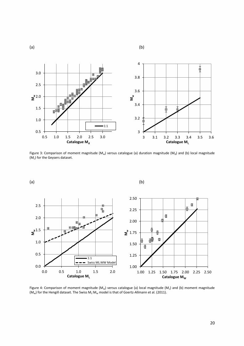
Comparing the remaining catalogue magnitudes with Mw we find that the duration magnitude (Md)

used by the Berkeley-Geysers (BG) network scales well with Mw (Figure 3), with R² = 0.98, but with a

constant offset. Using an L2 minimization, assuming known Md, we find that for the Geysers

catalogue in the range 0.9≤Md≤3:

(4)

Catalogue ML values (although there are few in this case) tend to be slightly lower than Mw, opposite

to the results for the Basel data in this magnitude range (Figure 3b).

The largest magnitude determined in our analysis was Mw 3.9. The offset of ML versus Mw in Figure 3

suggests this is anonymously high. A corresponding value from the NCSN was not available. However,

using the empirical GMPEs derived by Douglas et al. (2013) for induced seismicity we can see that a

mean value of Mw 3.9 is consistent with recorded peak ground velocity (PGV) for this event. Similarly,

upon recomputing ML for this event we find a higher value of 4.4, which is then more consistent with

the general trend.

3.3 Hengill, Iceland

Data from induced earthquakes related to the Hengill geothermal area were recorded as part of the

I-GET FP6 project (Jousset et al., 2011). The temporary array consisted of seven Guralp Systems

broadband seismometers. The dataset was supplemented by recordings from three 5s Lennarz

velocimeters of the Iceland Meteorological Office (IMO). Seismicity is thought to be related to

cooling and subsequent contraction of the rock (Jousset et al., 2011). κ0 values were first measured

for each station. From this the average amplification was estimated to be a factor of 2.1 using

equation (2). Computed Mw values are shown in Figure 4, compared with catalogue values for local

and moment magnitude from IMO. An offset of around 0.3 units between the Mw value determined

here and the catalogue values is apparent. The inverted Mw values also fall above the ML:Mw trend

line of Goertz-Allmann et al. (2011). Such a systematic difference suggests that the magnitudes were

computed using different assumptions. A particularly sensitive choice is the attenuation correction.

10

In our computation, we used the simplest assumption of 1/R decay; however, given adequate

knowledge of local attenuation, this may have been assigned differently.

3.4 Roswinkel, Netherlands

Roswinkel is the location of a natural gas-field in north-east Netherlands. The gas field is situated at a

depth of around 2 km and was exploited between 1980 and 2005. The strongest earthquake

recorded was an ML 3.4 event, which led to shaking equivalent to macroseismic intensity VI. Our

dataset consists of 27 events with 0.9≤ML≤3.2 recorded by up to five strong-motion sensors

deployed to record the seismicity related to the gas-field. Of these, 24 were assigned Mw values.

Unfortunately, most events were well recorded by only one to three instruments which may lead to

large deviations in magnitude estimation due to radiation effects. Nevertheless, the plot of Mw

versus catalogue ML shows a surprisingly linear scaling, with minimal scatter (Figure 5). Additionally,

the magnitudes conform quite closely to the Swiss Mw:ML scaling relation of Goertz-Allmann et al.

(2011), with a constant offset of around 0.1 units.

3.5 Soultz, France

The Soultz dataset is from a research EGS project situated in the Rhine Graben. Data are obtained

from three velocimeters, which recorded numerous earthquakes induced over the course of several

reservoir stimulation phases between 2003 and 2010. The main reservoir is located at around 5km

depth and is at approximately 200°C. We analyse data from the 2003 injection phase. From the

measured κ of 0.03s, it was estimated using Equation (2) that the average amplification would be a

factor of 2.1. The inversion showed that amplification was similar at all three instrumentation sites

(2.6, 1.8 and 2.0), probably due to their close proximity on similar geology. A comparison of

catalogue ML (provided by l'École et Observatoire des Sciences de la Terre, EOST) versus inverted MW

values is shown in Figure 6. In this case, the catalogue ML values are generally higher than MW, and

deviate by over 0.5 units from the Swiss Mw:ML scaling relation. One explanation for this could be

related to the very short recording distances for this data. In this case, the correct calibration of the

11

ML scale at such distance is critical, and may be overlooked if regional seismicity was used for its

derivation.

3.6 Cooper Basin, Australia

Cooper Basin lies in central Australia and is home to significant oil and gas production. A recent EGS

experiment in 2003 was performed by injecting more than 20,000 m³ of water into the Granitic crust

at 4.25 km depth (Baisch et al., 2006). Thousands of induced events were detected and recorded by

an eight station three-component geophone network deployed in boreholes at depths between 70

and 1700 m (Baisch et al., 2006). The limited instrument sensitivity presents a challenge in this case;

with the corner-frequency of the instrument’s velocity-response at around 10Hz. Nevertheless, due

to the relatively low-attenuation (recordings at short distance), and small magnitude, the spectral-

plateaus could still be reliably measured. Mw could, therefore, still be determined despite the

strongly band-limited data. Attenuation was measured as between κ=0.02 and 0.04s, which is not

particularly low, despite the borehole installations. This is probably because, despite the sensors

being located in boreholes, the limited penetration depths did not exceed the limit of the

sedimentary basin. Based on the observed attenuation, average amplification was estimated to be a

factor of 2.3. Inverted values were consistent with borehole depths: the shallower boreholes (90-

110m) generally leading to higher recorded amplification than the deeper boreholes (220-450m),

with factors of 3.6 and 1.1 respectively. In this case, we also accounted for the fact that the borehole

sensors are not subject to the free-surface effect (roughly a factor of two). The computed Mw (Figure

7) are systematically lower than Mw and lie above the Swiss ML:Mw relation by about 0.3 units. The

largest event in our database had ML 2.5, and was assigned as Mw 2.9. In this case, we suspect that

the significantly band-limited instrument led to the underestimation of ML.

4 Common Local Magnitude and Mequiv

In the previous section, we compared catalogue magnitudes with computed Mw. Significant and

systematic variations could be seen across the different datasets. This obviously has an impact on

12

the estimated hazard if a single ground motion prediction equation (GMPE) is used in all cases. An

important question to pose is: whether such differences are really justified, or whether they arise

purely from processing and computational decisions? In order to make a meaningful comparison

between the datasets, we recomputed all ML using a common correction for attenuation. This makes

a similar assumption to that used for our Mw calculation: regional differences in attenuation have a

low influence for short propagation distances. The equation used was as Equation (1), with A the

displacement in mm on a Wood-Anderson Torsion Seismometer (here simulated), along with the

attenuation correction used by the Southern California Seismic Network:

[ ] (5)

which is modified from Kanamori et al. (1993) . The resulting comparison with Mw is shown in Figure

8. Two subsets are apparent: those events which follow the model of Goertz-Allmann et al. (2011):

Geysers, Hengill and Basel (Figure 8a); and those which follow the same trend, but offset by around

half a magnitude unit: Roswinkel and Soultz (Figure 8b). Interestingly, Roswinkel has shifted from

presenting positive Mw-ML residuals, to negative, highlighting that magnitudes are not absolute.

Edwards et al. (2010) and Deichmann (2006) showed, through numerical simulations, that

differences in frequency dependent attenuation (e.g., Q and κ) have the most impact in scaling

between ML and Mw at low magnitudes, since, despite differences in stress-parameter, such events

all have significant proportions of high-frequency energy at the source. As such, we would suspect

that the two subsets of events exhibiting similar scaling behaviour undergo similar attenuation.

Between the two, we could then infer that attenuation at Geysers, Hengill and Basel is higher than at

Roswinkel (relative to the correction applied using Equation (5)). However, a further problem is

apparent, and that is the non-uniform distance distribution between individual databases.

Unfortunately, this could reflect discrepancies or bias in the distance-attenuation correction. For

instance, Roswinkel and Soultz (comprising one of the subsets) have very short average distances of

about 3 and 5km, respectively.

13

Bommer et al. (2006) introduced the concept of a PGV-referenced magnitude as part of their traffic-

light alert system for EGS projects, using the example of Berlin, El Salvador. The PGV-equivalent

magnitude (Mequiv), for a reference hypocentral depth was defined to be the event magnitude

required for an event at that depth to produce the same surface PGV, according to a prescribed

attenuation equation. In order to define the attenuation equation, we regressed Mw (to estimate

Mequiv), PGV and hypocentral distance using an equation of the form:

√ (6)

with R the hypocentral distance, and PGV in ms-1. All datasets with the exception of Cooper Basin

(because of the limited bandwidth of its data) were included in the regression. We found that

3.9720; 2.1577 and 4.6403, with 0.82. Unfortunately, the rather large indicates

that there is limited correspondence between Mw and PGV, at least using the functional form

adopted. This may be due to the role of source properties (such as slip kinematics or stress-drop),

which do not affect Mw, but have a significant impact on recorded PGV, particularly in the case of

weakly attenuated signals. Whilst the minimisation aimed to reduce the misfit between moment and

PGV-equivalent magnitude, PGV is nevertheless a point-measure on a seismogram. Therefore, it is

not surprising that it behaves similarly to ML, another point- and band-limited measure, as shown in

Figure 9. This similarity in scaling can be seen in Figure 10, which shows Mequiv versus recalculated ML.

It can again be noticed that the data fall into the same two distinct subgroups.

Since in this case, the attenuation correction was specifically designed for the data (as opposed to

the correction adopted for Southern California in the case of ML). We can infer (after checking the

residuals of the regression) that it is not a result of any bias in the distance correction which leads to

the difference in ML:Mw scaling. Rather, the difference must be a result of either: (a) different

attenuation, or (b) different source properties in the different regions, or indeed, a combination of

both.

14

5 Conclusion

We computed moment magnitude for induced earthquakes from a number of regions. Comparing

these against catalogue magnitudes, we found that they all broadly follow similar scaling behaviour,

but offset relative to one another. This scaling behaviour was found to follow a segmented

polynomial curve, consistent with the results of Goertz-Allmann et al. (2011). The scatter of all

catalogue ML values versus Mw was significant, which leads us to question what reported earthquake

magnitudes really tell us, and how they can be used in hazard assessments?

Part of the problem is through agency specific calibration of the ML scale, for example, how

attenuation is accounted for. This was highlighted by Fäh et al. (2011) during a catalogue

homogenization for the Earthquake Catalogue of Switzerland 2009: events occurring in the border

regions of Switzerland would be assigned systematically different magnitudes by the seismological

observatories operating on either side of the border. Clearly, some differences in attenuation

corrections may be justified. However, in order to compare all events independently of source

agency, we recomputed the ML values using a Californian attenuation model. In this case, with the

same data used for the computation of ML and Mw, and a unique attenuation correction, the scatter

in the scaling plots was significantly reduced. Nevertheless, two sub-classes of events were apparent,

the first with scaling exactly following the model of Goertz-Allmann et al. (2011), and a second with

approximately a half unit offset. This observation itself may indicate that the two sub-groups require

different attenuation corrections or calibration of the computation of ML from Wood-Anderson

amplitudes. Edwards et al. (2010) showed through simulated seismograms that the curvature of

ML:MW scaling is strongly controlled by source scaling (i.e., how stress-drop varies with Mw). The

similarity in shape of the ML:MW scaling in both subgroups indicates that average source-scaling is

therefore similar in all regions.

What is important to note is that due to the control of ML by relatively high frequencies (compared

to Mw), it is more sensitive to differences in attenuation. This fact, and the resultant ambiguity in the

15

meaning of ML, leads us to suggest that it is not suitable for ground-motion prediction or PSHA

where components (GMPEs, recurrence statistics, etc.) are adopted from other regions. Similarly, we

do not recommend that Mw is estimated from ML, apart from in the case that the conversion

equation is robustly determined from local (network specific) data (e.g., Douglas et al., 2013). The

magnitudes from the Cooper basin data were not included in this analysis, as we could not be sure

that the significantly-limited instrument bandwidth (f>10Hz) did not have an adverse impact on

estimated ML. This highlights the importance of monitoring decisions: while low-cost geophones are

suitable for detection and location, magnitude estimation requires recording in a suitable frequency

bandwidth.

Finally, we computed a PGV-equivalent magnitude, Mequiv, using an attenuation model computed

using the data of this study. It was shown that ML and Mequiv scale 1:1, although offsets are apparent

within particular datasets. This suggests a systematic difference in the PGV of records from a certain

dataset, with respect to the Wood-Anderson response, and may be indicative of underlying source-

or attenuation processes. Due to the 1:1 scaling of ML and Mequiv, the scaling of Mw with Mequiv was

similar to that observed for ML: with two distinct sub-classes. Since the attenuation correction for

PGV was computed using data from many regions, we could eliminate the influence of inappropriate

distance correction interacting with different average recording distances. As a result, we inferred

that the ground motion recorded in the various regions (Geysers, Hengill and Basel versus Soultz and

Roswinkel) is fundamentally different, either due to different source-, and/or different regional

attenuation-processes.

In the case of a probabilistic or deterministic hazard analysis for an EGS project, the expected

earthquake magnitude distribution is required as an input. We have seen here, that if all ML values

are taken as equal, it would have a significant impact on the hazard calculated in different regions. In

fact, after recomputing ML we saw that differences with respect to our reference Mw were quite

limited. The important aspect to consider is the compatibility of the magnitude computation (and

16

resulting distribution), the GMPE to be used in the hazard analysis and the observed data. What

must be avoided, is for equations to be chosen ad-hoc (e.g., ML attenuation corrections, or

conversion from ML to Mw), without consideration of the propagation of errors due to such decisions

further down the line. Finally, we recommend that magnitudes are properly defined, and that they

are calibrated with a suitable GMPE (e.g., Douglas et al., 2013), such that in the case of hazard

analysis, correct spectral ordinates can be properly estimated.

Acknowledgements

This study was partially funded by GEISER (Geothermal Engineering Integrating Mitigation of Induced

Seismicity in Reservoirs) project funded under contract 241321 of the EC-Research Seventh

Framework Programme (FP7). We thank Philippe Jousset for providing the data from Hengill; Michel

Frogneux for the data from Soultz; Lawrence Berkeley National Laboratory Geysers/Calpine seismic

network and NCEDC for the data from The Geysers; KNMI for the data from Roswinkel; the Swiss

Seismological Service and Geothermal Explorers Ltd. for the data from Basel and Geodynamics Ltd.

(Australia) for the data from Cooper Basin. We thank Lawrence Hutchings and Ernest Majer for their

reviews, which led to improvements to the clarity of this article.

References

Anderson, J. G. and S. E. Hough (1984). A Model for the Shape of the Fourier Amplitude Spectrum of Acceleration at High-Frequencies, Bulletin of the Seismological Society of America 74, 1969-1993.

Baisch, S., R. Weidler, R. Voros, D. Wyborn and L. de Graaf (2006). Induced seismicity during the stimulation of a geothermal HFR reservoir in the Cooper Basin, Australia, Bulletin of the Seismological Society of America 96, 2242-2256.

Bazzurro, P. and C. A. Cornell (1999). Disaggregation of seismic hazard, Bulletin of the Seismological Society of America 89, 501-520.

Bethmann, F., N. Deichmann and P. M. Mai (2012). Seismic wave attenuation from borehole and surface records in the top 2.5 km beneath the city of Basel, Switzerland, Geophysical Journal International 190, 1257-1270.

Bommer, J. J., S. Oates, J. M. Cepeda, C. Lindholm, J. Bird, R. Torres, G. Marroquin and J. Rivas (2006). Control of hazard due to seismicity induced by a hot fractured rock geothermal project, Engineering Geology 83, 287-306.

Borcherdt, R. D. (1994). Estimates of site-dependent response spectra for design (methodology and justification), Earthquake Spectra 10, 617-617.

17

Brune, J. N. (1970). Tectonic Stress and Spectra of Seismic Shear Waves from Earthquakes, Journal of Geophysical Research 75, 4997-&.

Brune, J. N. (1971). Correction, Journal of Geophysical Research 76, 5002-&. Deichmann, N. (2006). Local magnitude, a moment revisited, Bulletin of the Seismological Society of

America 96, 1267-1277. Deichmann, N. and D. Giardini (2009). Earthquakes Induced by the Stimulation of an Enhanced

Geothermal System below Basel (Switzerland), Seismological Research Letters 80, 784-798. Douglas, J., B. Edwards, B. M. Cabrera, V. Convertito, A. Tramelli, D. Kraaijpoel, N. Maercklin, N.

Sharma and G. De Natale (2013). Predicting ground motion from induced earthquakes in geothermal areas, Bulletin of the Seismological Society of America 103.

Edwards, B., B. Allmann, D. Fäh and J. Clinton (2010). Automatic computation of moment magnitudes for small earthquakes and the scaling of local to moment magnitude, Geophysical Journal International 183, 407-420.

Edwards, B., D. Fäh and D. Giardini (2011). Attenuation of seismic shear wave energy in Switzerland, Geophysical Journal International 185, 967-984.

Edwards, B., C. Michel, V. Poggi and F. D. (2013). Determination of Site Amplification from Regional Seismicity: Application to the Swiss National Seismic Networks. Accepted for publication in Seismological Research Letters.

Fäh, D., D. Giardini, P. Kästli, N. Deichmann, M. Gisler, G. Schwarz-Zanetti, S. Alvarez-Rubio, S. Sellami, B. Edwards and B. Allmann (2011). ECOS-09 Earthquake Catalogue of Switzerland Release 2011 Report and Database. Public catalogue, 17. 4. 2011. Swiss Seismological Service ETH ZurichReport SED/RISK.

Giardini, D. (2009). Geothermal quake risks must be faced, Nature 462, 848-849. Goertz-Allmann, B. P., B. Edwards, F. Bethmann, N. Deichmann, J. Clinton, D. Fah and D. Giardini

(2011). A New Empirical Magnitude Scaling Relation for Switzerland, Bulletin of the Seismological Society of America 101, 3088-3095.

Grünthal, G., R. Wahlstrom and D. Stromeyer (2009). The unified catalogue of earthquakes in central, northern, and northwestern Europe (CENEC)-updated and expanded to the last millennium, Journal of Seismology 13, 517-541.

Gutenberg, B. and C. F. Richter (1944). Frequency of earthquakes in California, Bulletin of the Seismological Society of America 34, 185-188.

Häring, M. O., U. Schanz, F. Ladner and B. C. Dyer (2008). Characterisation of the Basel 1 enhanced geothermal system, Geothermics 37, 469-495.

Jousset, P., C. Haberland, K. Bauer and K. Arnason (2011). Hengill geothermal volcanic complex (Iceland) characterized by integrated geophysical observations, Geothermics 40, 1-24.

Kanamori, H., J. Mori, E. Hauksson, T. H. Heaton, L. K. Hutton and L. M. Jones (1993). Determination of earthquake energy release and ML using TERRAscope, Bulletin of the Seismological Society of America 83, 330-346.

Majer, E. L., R. Baria, M. Stark, S. Oates, J. Bommer, B. Smith and H. Asanuma (2007). Induced seismicity associated with enhanced geothermal systems, Geothermics 36, 185-222.

Poggi, V., B. Edwards and D. Fäh (2011). Derivation of a Reference Shear-Wave Velocity Model from Empirical Site Amplification, Bulletin of the Seismological Society of America 101, 258-274.

Richter, C. F. (1935). An instrumental earthquake magnitude scale, Bulletin of the Seismological Society of America 25, 1-32.

18

List of Figure Captions

Figure 1: Comparison of moment magnitude (Mw) versus (a) local magnitude (ML) and (b) Earthquake

catalogue of Switzerland 2009 (ECOS09) Mw for the Basel EGS dataset. The Swiss ML:Mw scaling

relation of Goertz-Allmann et al. (2011) is shown.

Figure 2: Comparison between inverted and catalogue Mw values for Geysers, showing those events

with fixed Mw.

Figure 3: Comparison of moment magnitude (Mw) versus catalogue (a) duration magnitude (Md) and

(b) local magnitude (ML) for the Geysers dataset.

Figure 4: Comparison of moment magnitude (Mw) versus catalogue (a) local magnitude (ML) and (b)

moment magnitude (Mw) for the Hengill dataset. The Swiss ML:Mw model is that of Goertz-Allmann

et al. (2011).

Figure 5: Comparison of moment magnitude (Mw) versus catalogue local magnitude (ML) for the

Roswinkel dataset. The Swiss ML:Mw model is that of Goertz-Allmann et al. (2011).

Figure 6: Comparison of moment magnitude (Mw) versus catalogue local magnitude (ML) for the

Soultz dataset. The Swiss ML:Mw model is that of Goertz-Allmann et al. (2011).

Figure 7: Comparison of moment magnitude (Mw) versus catalogue local magnitude (ML) for the

Cooper Basin dataset. The Swiss ML:Mw model is that of Goertz-Allmann et al. (2011).

Figure 8: Comparison of common ML scale versus inverted Mw for all datasets in the study. (a)

Geysers, Hengill and Basel events, along with the Swiss ML:Mw model of Goertz-Allmann et al. (2011).

(b) Roswinkel and Soultz events plotted along with the Swiss ML:Mw model offset by 0.5 units.

Figure 9: Comparison of common Mequiv versus inverted Mw for all datasets in the study. (a) Geysers,

Hengill and Basel events. (b) Roswinkel and Soultz events.

Figure 10: Comparison of ML using the Southern California attenuation, with Mequiv.

19

Figures

(a) (b)

Figure 1: Comparison of moment magnitude (Mw) versus (a) local magnitude (ML) and (b) Earthquake catalogue of Switzerland 2009 (ECOS09) Mw for the Basel EGS dataset. The Swiss ML:Mw scaling relation of Goertz-Allmann et al. (2011) is shown.

Figure 2: Comparison between inverted and catalogue Mw values for Geysers, showing those events with fixed Mw.

0.5

1.0

1.5

2.0

2.5

3.0

3.5

0.5 1.0 1.5 2.0 2.5 3.0 3.5

Mw

Catalogue ML

1:1

Swiss ML:MW-0.6

-0.4

-0.2

0.0

0.2

0.4

0.6

1.0 1.5 2.0 2.5 3.0 3.5M

w D

iffe

ren

ce (

Inve

rte

d -

EC

OS0

9)

Catalog Mw (Converted) (ECOS09)

3

3.1

3.2

3.3

3.4

3.5

3.6

3.7

3.8

3.9

3 3.1 3.2 3.3 3.4 3.5 3.6 3.7 3.8 3.9

Mw

Catalogue Mw

Inv Mw

Fixed Mw

1:1

20

(a) (b)

Figure 3: Comparison of moment magnitude (Mw) versus catalogue (a) duration magnitude (Md) and (b) local magnitude (ML) for the Geysers dataset.

(a) (b)

Figure 4: Comparison of moment magnitude (Mw) versus catalogue (a) local magnitude (ML) and (b) moment magnitude (Mw) for the Hengill dataset. The Swiss ML:Mw model is that of Goertz-Allmann et al. (2011).

0.5

1.0

1.5

2.0

2.5

3.0

0.5 1.0 1.5 2.0 2.5 3.0

Mw

Catalogue Md

1:1

3

3.2

3.4

3.6

3.8

4

3 3.1 3.2 3.3 3.4 3.5 3.6

Mw

Catalogue ML

0.0

0.5

1.0

1.5

2.0

2.5

0.0 0.5 1.0 1.5 2.0

Mw

Catalogue ML

1:1

Swiss ML:MW Model

1.00

1.25

1.50

1.75

2.00

2.25

2.50

1.00 1.25 1.50 1.75 2.00 2.25 2.50

Mw

Catalogue MW

21

Figure 5: Comparison of moment magnitude (Mw) versus catalogue local magnitude (ML) for the Roswinkel dataset. The Swiss ML:Mw model is that of Goertz-Allmann et al. (2011).

Figure 6: Comparison of moment magnitude (Mw) versus catalogue local magnitude (ML) for the Soultz dataset. The Swiss ML:Mw model is that of Goertz-Allmann et al. (2011).

0.5

1.0

1.5

2.0

2.5

3.0

3.5

0.5 1.0 1.5 2.0 2.5 3.0 3.5

Mw

Catalogue ML

1:1

Swiss ML:MW Model

1.0

1.5

2.0

2.5

3.0

1.0 1.5 2.0 2.5 3.0

Mw

Catalogue ML

1:1

Swiss ML:MW Model

22

Figure 7: Comparison of moment magnitude (Mw) versus catalogue local magnitude (ML) for the Cooper Basin dataset. The Swiss ML:Mw model is that of Goertz-Allmann et al. (2011).

(a) (b)

Figure 8: Comparison of common ML scale versus inverted Mw for all datasets in the study. (a) Geysers, Hengill and Basel events, along with the Swiss ML:Mw model of Goertz-Allmann et al. (2011). (b) Roswinkel and Soultz events plotted along with the Swiss ML:Mw model offset by 0.5 units.

0.5

1.0

1.5

2.0

2.5

3.0

0.5 1.0 1.5 2.0 2.5 3.0

Mw

Catalogue ML

1:1

Swiss ML:Mw Model

0.5

1.0

1.5

2.0

2.5

3.0

3.5

4.0

4.5

5.0

0.5 1.0 1.5 2.0 2.5 3.0 3.5 4.0 4.5 5.0

Mw

California ML

Geysers

Hengill

Basel

1:1

Swiss ML:Mw model0.5

1.0

1.5

2.0

2.5

3.0

3.5

4.0

4.5

5.0

0.5 1.0 1.5 2.0 2.5 3.0 3.5 4.0 4.5 5.0

Mw

California ML

RoswinkelSoultz1:1Swiss ML:Mw - 0.5

23

(a) (b)

Figure 9: Comparison of common Mequiv versus inverted Mw for all datasets in the study. (a) Geysers, Hengill and Basel events. (b) Roswinkel and Soultz events.

Figure 10: Comparison of ML using the Southern California attenuation, with Mequiv.

0.5

1.0

1.5

2.0

2.5

3.0

3.5

4.0

4.5

5.0

0.5 1.0 1.5 2.0 2.5 3.0 3.5 4.0 4.5 5.0

Mw

Mequiv

Geysers

Hengill

Basel

1:1

0.5

1.0

1.5

2.0

2.5

3.0

3.5

4.0

4.5

5.0

0.5 1.0 1.5 2.0 2.5 3.0 3.5 4.0 4.5 5.0

Mw

Mequiv

Roswinkel

Soultz

1:1

0.5

1.0

1.5

2.0

2.5

3.0

3.5

4.0

4.5

5.0

0.5 1.0 1.5 2.0 2.5 3.0 3.5 4.0 4.5 5.0

Cal

ifo

rnia

ML

Mequiv

Geysers

Roswinkel

Hengill

Basel

Soultz

1:1