the magnitude distribution of earthquakes near southern

The magnitude distribution of earthquakes nearSouthern California faults

Morgan T. Page,1 David Alderson,2 and John Doyle3

Received 14 August 2010; revised 16 September 2011; accepted 28 September 2011; published 16 December 2011.

[1] We investigate seismicity near faults in the Southern California Earthquake CenterCommunity Fault Model. We search for anomalously large events that might be signs of acharacteristic earthquake distribution. We find that seismicity near major fault zones inSouthern California is well modeled by a Gutenberg-Richter distribution, with no evidenceof characteristic earthquakes within the resolution limits of the modern instrumentalcatalog. However, the b value of the locally observed magnitude distribution is found todepend on distance to the nearest mapped fault segment, which suggests that earthquakesnucleating near major faults are likely to have larger magnitudes relative to earthquakesnucleating far from major faults.

Citation: Page, M. T., D. Alderson, and J. Doyle (2011), The magnitude distribution of earthquakes near Southern Californiafaults, J. Geophys. Res., 116, B12309, doi:10.1029/2010JB007933.

1. Introduction

[2] It is well known that earthquake magnitudes withinlarge regions follow the Gutenberg-Richter (G-R) distribu-tion. The Gutenberg-Richter magnitude distribution relatesthe cumulative number of earthquakes N above a givenmagnitude, M, by

log Nð Þ ¼ a � bM ; ð1Þ

where a and b are constants [Ishimoto and Iida, 1939;Gutenberg and Richter, 1944]. The b value is generallyapproximately 1 [Frohlich and Davis, 1993], which means,in combination with constant stress drop scaling [e.g., Aki,1972], that the number of earthquakes in a given magni-tude range is proportional to the reciprocal of the fault rup-ture area. For California, b = 1 matches the modern catalogwell [Felzer, 2008; Hutton et al., 2010].[3] While the Gutenberg-Richter distribution is used to

model seismicity in large regions, there is some question asto whether it applies to earthquakes in individual fault zones.The characteristic magnitude distribution [Wesnousky et al.,1983; Schwartz and Coppersmith, 1984; Wesnousky, 1994]alternatively holds that large earthquakes in major faultzones occur at a higher rate relative to smaller earthquakesthan the Gutenberg-Richter distribution would predict. Thecharacteristic magnitude distribution has been suggested inpart because of an apparent mismatch between paleoinferredrates of large earthquakes on major faults and rates of smallerearthquakes from the instrumental catalog for a narrow

region surrounding the fault. In this work we consider onlythe modern instrumental catalog, for which hypocenters areknown and magnitudes are well characterized. This choicewill limit the size of the catalog and therefore the highestmagnitudes available; however, including data from manyfaults throughout California, rather than studying a singlefault zone, improves the power of our tests considerably.[4] The characteristic magnitude distribution is often

used in seismic hazard analysis [e.g., Working Group onCalifornia Earthquake Probabilities, 1990a, 1990b, 1995,1999; Field et al., 2008]. However, the use of the character-istic earthquake model can lead to some difficulty in match-ing regional catalog rates. On a state-wide basis, magnitudesare G-R distributed, and it can be difficult to produce anoverall catalog that matches the G-R distribution whenseismicity on individual faults is modeled with a charac-teristic distribution. Previous statewide hazard models forCalifornia have contained discrepancies between historicearthquake rates and rates given by the model betweenmagnitudes 6 and 7 [Field et al., 1999; Petersen et al., 2000].Significant tinkering with model parameters has beenrequired to alleviate what has colloquially become known asthe “battle of the bulge” [Field et al., 2008].[5] Inherent in the characteristic earthquake hypothesis is

a scaling break between the large and small events on agiven fault. Southern California is a good place to look forsuch a scaling break, if it exists, since there are earthquakecatalogs of well-located earthquakes with well-characterizedmagnitudes and digital models of 3-D fault surfaces in theregion. We investigate the magnitude distribution of earth-quakes near major fault zones in Southern California todetermine if the largest events in fault zones are larger thanwould be predicted by a Gutenberg-Richter distribution. Webegin by examining seismicity near the Parkfield section ofthe San Andreas Fault before extending our analysis to allmajor mapped fault zones in Southern California. We alsolook for changes in the magnitude distribution with distance

1U.S. Geological Survey, Pasadena, California, USA.2Operations Research Department, Naval Postgraduate School,

Monterey, California, USA.3Control and Dynamical Systems, California Institute of Technology,

Pasadena, California, USA.

Copyright 2011 by the American Geophysical Union.0148-0227/11/2010JB007933

JOURNAL OF GEOPHYSICAL RESEARCH, VOL. 116, B12309, doi:10.1029/2010JB007933, 2011

B12309 1 of 9

http://dx.doi.org/10.1029/2010JB007933

from major fault zones, to see if the catalog contains dif-ferences between major fault seismicity and regional seis-micity that are often assumed in seismic hazard models.

2. Seismicity Near Parkfield

[6] The Parkfield section of the San Andreas Fault hasbeen hypothesized to rupture in quasiperiodic “characteris-tic” events of approximately magnitude 6 [Bakun and Lindh,1985; Jackson and Kagan, 2006]. We do not consider timedependence in this study, but focus instead on the magnitudedistribution for this fault section. Is there an increase in M6earthquakes near Parkfield, beyond what would be consis-tent with G-R statistics?[7] Figure 1a shows the cumulative magnitude distribu-

tion for Parkfield section earthquakes. Events are includedfrom the ANSS catalog, 1984–2007, within 5 km of the faulttrace, as defined by the Working Group on CaliforniaEarthquake Probabilities [Field et al., 2008]. Comparingdirectly to a best fit G-R curve, the G-R distribution appears

to severely underpredict the rate of M6 earthquakes. Evenaccounting for b value error (95% confidence bounds for theb value are determined by maximum likelihood [Aki, 1965]does not account for this apparent overprediction. It is easyto see from Figure 1a one reason for the development of thecharacteristic earthquake hypothesis.[8] However, this simple analysis fails to account for the

inherent variability in the tail of the distribution wheresampling error becomes important. We can see this bygenerating 20 random sets of magnitudes drawn from theGutenberg-Richter distribution, each with the same numberof events as the Parkfield data set (Figure 1b). These samplesshow that variability in the tail of the power law distributionis the rule rather than the exception. In fact, considering thisvariability, the rate of M6 events in Parkfield is consistentwith a b = 1 G-R distribution at 95% confidence (the exact95% confidence bounds for each point in the curve areshown with the shading in Figure 1b).

3. Magnitude Distributions in Individual FaultZones

[9] We systematically extend our analysis to all majormapped faults in Southern California. We assign earth-quakes, in 3D, to the nearest fault in the Southern CaliforniaEarthquake Center (SCEC) Community Fault Model (CFM),version 3.0. This is similar to the rCFM earthquake data-base [Woessner and Hauksson, 2006; Hauksson, 2010]which assigns earthquakes to the nearest fault as defined bythe rectilinear CFM version 2.5. The SCEC CFM version 3.0that we use in this analysis contains triangulated, nonplanarfault surfaces. Like the rCFM catalog, we use events fromthe Southern California Seismic Network from 1981 to 2004(inclusive), relocated using a double-difference method[Hauksson and Shearer, 2005]. We adjust the relocated cat-alog in two ways: (1) we replace the magnitudes with morerecent magnitudes from the Southern California SeismicNetwork (SCSN), and (2) we add missing events that are inthe SCSN catalog but absent from the older rCFM database.This gives a total of 26,479 earthquakes above magnitude 2.5and within 20 km of the CFM fault segments. Importantly,the revised data set includes the 1992 M7.3 Landers earth-quake, which is absent from the original relocated catalog.This earthquake is the largest earthquake in the revised dataset. The addition of missing events and the use of newerSCSN magnitudes do not significantly change the resultswe present here.[10] We separate the earthquakes into bins on the basis of

the fault zone to which each is assigned, which is the closestfault in the CFM (we calculate the closest distance in 3D,taking into account the depths of the events and the non-planar fault sources of the CFM 3.0). The faults themselvesare chosen (“segmented”) just as they are defined in theCFM. There is certainly some subjectivity in how segmentsare defined; this cannot be avoided, but we do not personallymodify the faults as defined by the community consensusCFM representation. The largest earthquakes in the catalogmay indeed rupture multiple segments, or even have hypo-centers located by the catalog some distance from the pri-mary rupture. We consider hypocenters only and do not useextended sources or assign large earthquakes to multiplesegments; this also prevents data selection on our part as

Figure 1. The cumulative magnitude distribution for earth-quakes within 5 km of the Parkfield section of the SanAndreas Fault is shown in blue. (a) An analysis of the bvalue error alone could lead to the erroneous conclusion thatthe largest events in this zone violate Gutenberg-Richter(G-R) behavior. (b) However, random samples drawn froma G-R distribution (black lines) demonstrate considerablescatter. The largest event is within the scatter predicted fromrandom G-R samples and thus does not violate the nullhypothesis that Parkfield earthquake magnitudes are drawnfrom a G-R distribution with a b value of 1.

PAGE ET AL.: MAGNITUDES NEAR SOUTHERN CALIFORNIA FAULTS B12309B12309

2 of 9

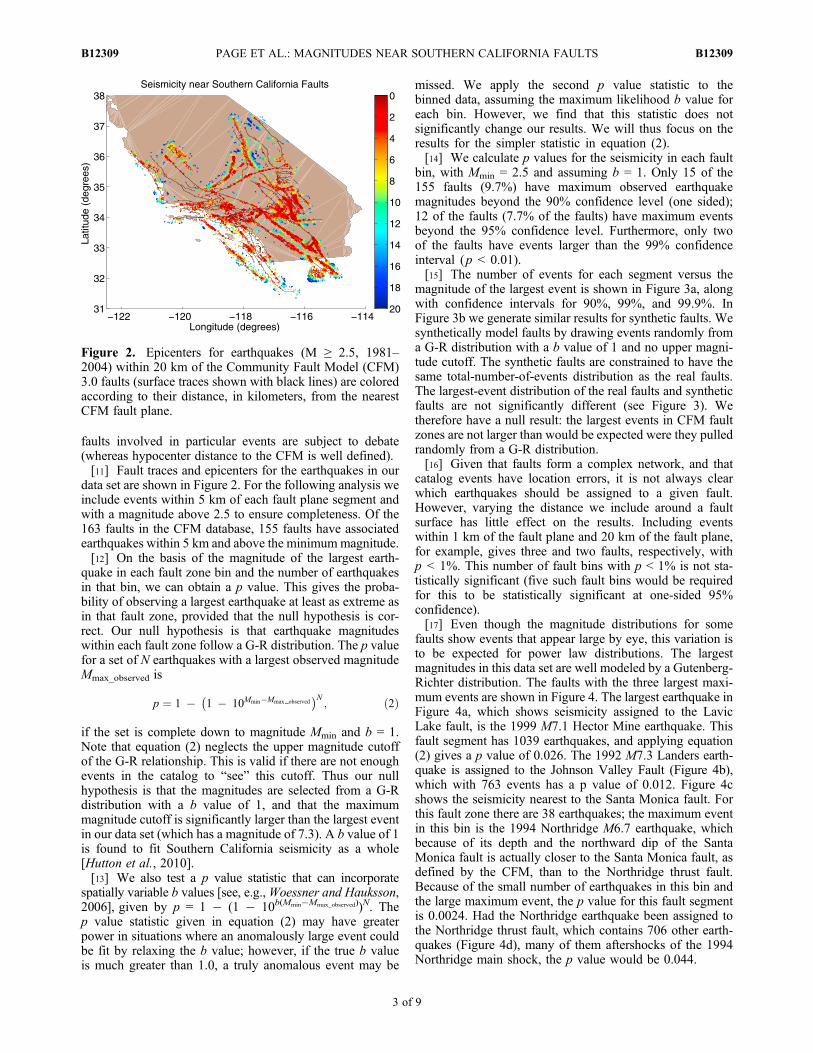
faults involved in particular events are subject to debate(whereas hypocenter distance to the CFM is well defined).[11] Fault traces and epicenters for the earthquakes in our

data set are shown in Figure 2. For the following analysis weinclude events within 5 km of each fault plane segment andwith a magnitude above 2.5 to ensure completeness. Of the163 faults in the CFM database, 155 faults have associatedearthquakes within 5 km and above the minimummagnitude.[12] On the basis of the magnitude of the largest earth-

quake in each fault zone bin and the number of earthquakesin that bin, we can obtain a p value. This gives the proba-bility of observing a largest earthquake at least as extreme asin that fault zone, provided that the null hypothesis is cor-rect. Our null hypothesis is that earthquake magnitudeswithin each fault zone follow a G-R distribution. The p valuefor a set of N earthquakes with a largest observed magnitudeMmax_observed is

p ¼ 1 � 1 � 10Mmin�Mmax observed� �N

; ð2Þ

if the set is complete down to magnitude Mmin and b = 1.Note that equation (2) neglects the upper magnitude cutoffof the G-R relationship. This is valid if there are not enoughevents in the catalog to “see” this cutoff. Thus our nullhypothesis is that the magnitudes are selected from a G-Rdistribution with a b value of 1, and that the maximummagnitude cutoff is significantly larger than the largest eventin our data set (which has a magnitude of 7.3). A b value of 1is found to fit Southern California seismicity as a whole[Hutton et al., 2010].[13] We also test a p value statistic that can incorporate

spatially variable b values [see, e.g.,Woessner and Hauksson,2006], given by p = 1 � (1 � 10b(Mmin�Mmax_observed))N. Thep value statistic given in equation (2) may have greaterpower in situations where an anomalously large event couldbe fit by relaxing the b value; however, if the true b valueis much greater than 1.0, a truly anomalous event may be

missed. We apply the second p value statistic to thebinned data, assuming the maximum likelihood b value foreach bin. However, we find that this statistic does notsignificantly change our results. We will thus focus on theresults for the simpler statistic in equation (2).[14] We calculate p values for the seismicity in each fault

bin, with Mmin = 2.5 and assuming b = 1. Only 15 of the155 faults (9.7%) have maximum observed earthquakemagnitudes beyond the 90% confidence level (one sided);12 of the faults (7.7% of the faults) have maximum eventsbeyond the 95% confidence level. Furthermore, only twoof the faults have events larger than the 99% confidenceinterval (p < 0.01).[15] The number of events for each segment versus the

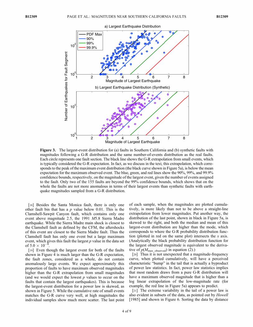
magnitude of the largest event is shown in Figure 3a, alongwith confidence intervals for 90%, 99%, and 99.9%. InFigure 3b we generate similar results for synthetic faults. Wesynthetically model faults by drawing events randomly froma G-R distribution with a b value of 1 and no upper magni-tude cutoff. The synthetic faults are constrained to have thesame total-number-of-events distribution as the real faults.The largest-event distribution of the real faults and syntheticfaults are not significantly different (see Figure 3). Wetherefore have a null result: the largest events in CFM faultzones are not larger than would be expected were they pulledrandomly from a G-R distribution.[16] Given that faults form a complex network, and that

catalog events have location errors, it is not always clearwhich earthquakes should be assigned to a given fault.However, varying the distance we include around a faultsurface has little effect on the results. Including eventswithin 1 km of the fault plane and 20 km of the fault plane,for example, gives three and two faults, respectively, withp < 1%. This number of fault bins with p < 1% is not sta-tistically significant (five such fault bins would be requiredfor this to be statistically significant at one-sided 95%confidence).[17] Even though the magnitude distributions for some

faults show events that appear large by eye, this variation isto be expected for power law distributions. The largestmagnitudes in this data set are well modeled by a Gutenberg-Richter distribution. The faults with the three largest maxi-mum events are shown in Figure 4. The largest earthquake inFigure 4a, which shows seismicity assigned to the LavicLake fault, is the 1999 M7.1 Hector Mine earthquake. Thisfault segment has 1039 earthquakes, and applying equation(2) gives a p value of 0.026. The 1992 M7.3 Landers earth-quake is assigned to the Johnson Valley Fault (Figure 4b),which with 763 events has a p value of 0.012. Figure 4cshows the seismicity nearest to the Santa Monica fault. Forthis fault zone there are 38 earthquakes; the maximum eventin this bin is the 1994 Northridge M6.7 earthquake, whichbecause of its depth and the northward dip of the SantaMonica fault is actually closer to the Santa Monica fault, asdefined by the CFM, than to the Northridge thrust fault.Because of the small number of earthquakes in this bin andthe large maximum event, the p value for this fault segmentis 0.0024. Had the Northridge earthquake been assigned tothe Northridge thrust fault, which contains 706 other earth-quakes (Figure 4d), many of them aftershocks of the 1994Northridge main shock, the p value would be 0.044.

Figure 2. Epicenters for earthquakes (M ≥ 2.5, 1981–2004) within 20 km of the Community Fault Model (CFM)3.0 faults (surface traces shown with black lines) are coloredaccording to their distance, in kilometers, from the nearestCFM fault plane.


3 of 9

[18] Besides the Santa Monica fault, there is only oneother fault bin that has a p value below 0.01. This is theClamshell-Sawpit Canyon fault, which contains only oneevent above magnitude 2.5, the 1991 M5.8 Sierra Madreearthquake. While the Sierra Madre main shock is closest tothe Clamshell fault as defined by the CFM, the aftershocksof this event are closest to the Sierra Madre fault. Thus theClamshell fault has only one event but a large maximumevent, which gives this fault the largest p value in the data setof 5.0 � 10�4.[19] Even though the largest event for both of the faults

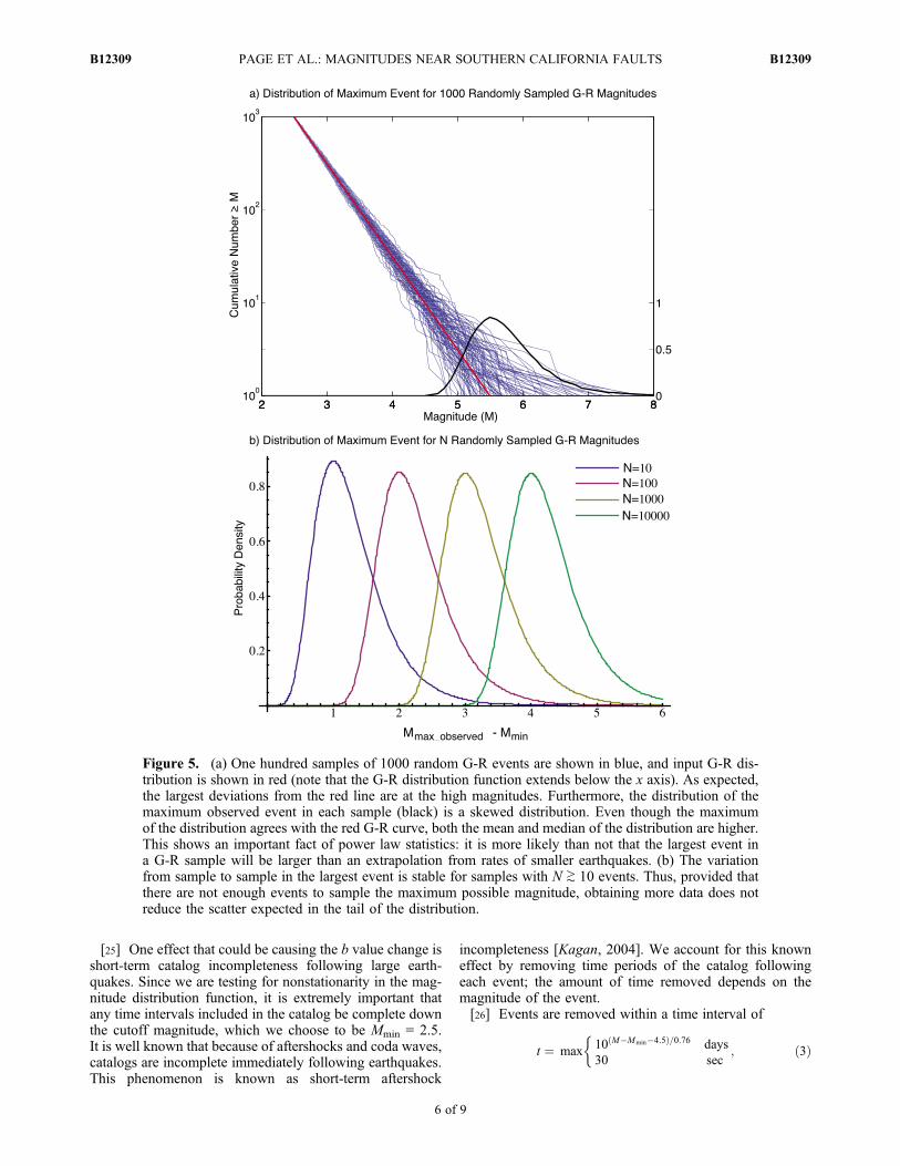
shown in Figure 4 is much larger than the G-R expectation,the fault zones, considered as a whole, do not containanomalously large events. We expect approximately thisproportion of faults to have maximum observed magnitudeshigher than the G-R extrapolation from small magnitudes(and we would expect the lowest p values to occur on thefaults that contain the largest earthquakes). This is becausethe largest-event distribution for a power law is skewed, asshown in Figure 5. While the cumulative rate of small eventsmatches the G-R curve very well, at high magnitudes theindividual samples show much more scatter. The last point

of each sample, when the magnitudes are plotted cumula-tively, is more likely than not to be above a straight-lineextrapolation from lower magnitudes. Put another way, thedistribution of the last point, shown in black in Figure 5a, isskewed to the right, and both the median and mean of thislargest-event distribution are higher than the mode, whichcorresponds to where the G-R probability distribution func-tion (plotted in red on the same plot) intersects the x axis.(Analytically the black probability distribution function forthe largest observed magnitude is equivalent to the deriva-tive of p(Mmax_observed) in equation (2).)[20] Thus it is not unexpected that a magnitude-frequency

curve, when plotted cumulatively, will have a perceivedcharacteristic “bump” in the tail that is actually a byproductof power law statistics. In fact, power law statistics impliesthat most random draws from a pure G-R distribution willhave a maximum observed magnitude that is higher than alog linear extrapolation of the low-magnitude rate (forexample, the red line in Figure 5a) appears to predict.[21] The extreme variability in the tail of a power law is

also evident in subsets of the data, as pointed out by Howell[1985] and shown in Figure 6. Sorting the data by distance

Figure 3. The largest-event distribution for (a) faults in Southern California and (b) synthetic faults withmagnitudes following a G-R distribution and the same number-of-events distribution as the real faults.Each circle represents one fault section. The black line shows the G-R extrapolation from small events, whichis typically considered the G-R expectation. In fact, as we discuss in the text, this extrapolation, which corre-sponds to the peak of the maximum event distribution (the black curve shown in Figure 5a), is below the meanexpectation for the maximum observed event. The blue, green, and red lines show the 90%, 99%, and 99.9%confidence bounds, respectively, on the magnitude of the largest event, given the number of events assignedto the fault. Only two of the 155 faults are beyond the 99% confidence bounds, which shows that on thewhole the faults are not more anomalous in terms of their largest events than synthetic faults with earth-quake magnitudes sampled from a G-R distribution.


4 of 9

from the CFM faults results in similar variability as therandom subsets shown in Figure 5a. In fact, this variability isnecessary; that is, one of the 10 subsets, on average, musthave a largest event a magnitude unit higher than a G-Rextrapolation from lower magnitudes if the total set ofearthquakes is to follow a G-R distribution as well (since adata set 10 times the size will have, on average, a largestobserved event 1 magnitude unit higher when b = 1). Thisvariability in the tail, interestingly, does not decrease withmore data until the data set is large enough to be affected bythe maximum possible magnitude for that region. This sta-bility of the largest-event distribution with respect to samplesize is shown in Figure 5b.

4. Magnitudes on the Fault Versus in the Bulk

[22] To what extent are earthquakes that nucleate on large,mapped faults different than earthquakes that nucleate onsmaller faults in the “bulk”? Certainly many of the faults arereadily apparent in seismicity locations; however, are thelarge, mapped faults apparent from other features of theseismicity, namely the magnitude distribution? Althoughthe major faults in California may accommodate much of thestrain release, it is another question whether large earth-quakes nucleate near the major faults, given the propensityfor faults to rupture together in single ruptures [Wesnousky,2008].[23] The extent to which magnitudes are sensitive to

nucleation location has important implications for hazardanalysis. If, for example, larger earthquakes are more likely

to nucleate closer to mapped faults, this would suggestincreased hazard from potential foreshocks located close tomajor faults relative to other regions [see, e.g., Agnew andJones, 1991]. Furthermore, if the magnitude distribution issensitive to the size of nearby faults, it also suggests that theG-R magnitude distribution we observe could be an effect ofthe fault network geometry.[24] The magnitude distribution of our catalog does, in

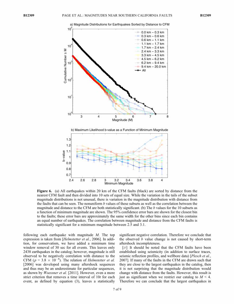
fact, change with distance from the CFM faults, as shownin Figure 6. The maximum likelihood b value for the 10%of earthquakes that are closest to the fault is 1.08 � 0.04at 95% confidence. By contrast the furthest bin from theCFM faults has a b value ranging from 1.15 to 1.24, at 95%confidence. The correlation (we use Pearson’s linear corre-lation in this paper) between the b values for the 10 binsshown in Figure 6a and the distance of the bins from theCFM faults is statistically significant. In addition, we canobtain an extremely statistically significant result whichdoes not rely on binning at all by calculating the correlationbetween the magnitude of each earthquake in the data setand its distance to the closest CFM fault. This correlation is�0.026 (it is negative because magnitudes tend to increaseas distance from the fault decreases). While this correlationmay seem small in the absolute sense (as is to be expectedgiven that the b values are not dramatically different) it is,in fact, significant at p = 3 � 10�5, as determined from ran-domly shuffled versions of the catalog. By increasing theminimum magnitude (see Figure 6b), we can remove enoughearthquakes so as to lose statistical significance; however,this does not happen for any Mmin ≤ 3.1.

Figure 4. (a–c) Cumulative magnitude-frequency distributions for the three faults with the largest earth-quakes in the data set. The G-R extrapolation with b = 1 is shown in red. While by eye these faults appearto contain anomalously large events, on the whole the largest-event distribution among the CFM faultsections is consistent with G-R behavior. (d) The 1994 M6.7 Northridge earthquake is located closer tothe Santa Monica fault than to the Northridge Thrust fault, as defined by the CFM 3.0; this results in amagnitude-frequency distribution for the Santa Monica fault that appears more anomalous because thesmaller aftershocks of the Northridge earthquake primarily locate on the Northridge Thrust. It shouldbe noted that picking out the faults with the largest earthquakes will naturally result in distributions thatappear to violate G-R behavior; however, this is a result of data selection, and when we analyze all thefaults, we find that the largest earthquakes do not violate G-R behavior.


5 of 9

[25] One effect that could be causing the b value change isshort-term catalog incompleteness following large earth-quakes. Since we are testing for nonstationarity in the mag-nitude distribution function, it is extremely important thatany time intervals included in the catalog be complete downthe cutoff magnitude, which we choose to be Mmin = 2.5.It is well known that because of aftershocks and coda waves,catalogs are incomplete immediately following earthquakes.This phenomenon is known as short-term aftershock

incompleteness [Kagan, 2004]. We account for this knowneffect by removing time periods of the catalog followingeach event; the amount of time removed depends on themagnitude of the event.[26] Events are removed within a time interval of

t ¼ max 10 M�Mmin�4:5ð Þ=0:76 days30 sec

;

�ð3Þ

Figure 5. (a) One hundred samples of 1000 random G-R events are shown in blue, and input G-R dis-tribution is shown in red (note that the G-R distribution function extends below the x axis). As expected,the largest deviations from the red line are at the high magnitudes. Furthermore, the distribution of themaximum observed event in each sample (black) is a skewed distribution. Even though the maximumof the distribution agrees with the red G-R curve, both the mean and median of the distribution are higher.This shows an important fact of power law statistics: it is more likely than not that the largest event ina G-R sample will be larger than an extrapolation from rates of smaller earthquakes. (b) The variationfrom sample to sample in the largest event is stable for samples with N ≳ 10 events. Thus, provided thatthere are not enough events to sample the maximum possible magnitude, obtaining more data does notreduce the scatter expected in the tail of the distribution.


6 of 9

following each earthquake with magnitude M. The topexpression is taken from [Helmstetter et al., 2006]. In addi-tion, for conservatism, we have added a minimum timewindow removal of 30 sec for all events. This leaves only2438 earthquakes in the catalog; however, magnitude is stillobserved to be negatively correlation with distance to theCFM (p = 3.8 � 10�4). The relation of Helmstetter et al.[2006] was developed using many aftershock sequencesand thus may be an underestimate for particular sequences,as shown by Woessner et al. [2011]. However, even a morestrict criterion that removes a time interval of 10t for eachevent, as defined by equation (3), leaves a statistically

significant negative correlation. Therefore we conclude thatthe observed b value change is not caused by short-termaftershock incompleteness.[27] It should be noted that the CFM faults have been

established using seismicity (in addition to surface traces,seismic reflection profiles, and wellbore data) [Plesch et al.,2007]. If many of the faults in the CFM are drawn such thatthey are close to the largest earthquakes in the catalog, thenit is not surprising that the magnitude distribution wouldchange with distance from the faults. However, this result isjust as significant when we restrict our catalog to M < 4.Therefore we can conclude that the largest earthquakes in

Figure 6. (a) All earthquakes within 20 km of the CFM faults (black) are sorted by distance from thenearest CFM fault and then divided into 10 sets of equal size. While the variation in the tails of the subsetmagnitude distributions is not unusual, there is variation in the magnitude distribution with distance fromthe faults that can be seen. The nonuniform b values of these subsets as well as the correlation between themagnitude and distance to the CFM are both statistically significant. (b) The b values for the 10 subsets asa function of minimum magnitude are shown. The 95% confidence error bars are shown for the closest binto the faults; these error bars are approximately the same width for the other bins since each bin containsan equal number of earthquakes. The correlation between magnitude and distance from the CFM faults isstatistically significant for a minimum magnitude between 2.5 and 3.1.


7 of 9

the catalog (M ≥ 4) are not driving this result. The best testto ensure that there is no circularity between the develop-ment of the CFM and changes in the magnitude distributionwith respect to it would be to perform these tests on theportion of the catalog developed post-CFM. Unfortunately,this version of the CFM was last updated in January 2004,which is roughly coincident with the end of our catalog.Newer relocated catalogs are not yet available; in the futurean updated catalog will allow one to test whether this effectis observed in seismicity not used to develop the CFM.

5. Discussion

[28] We observe highly statistically significant changes inb value with distance from the major faults in SouthernCalifornia, as defined by the CFM 3.0. If these observedb value changes are persistent in time (and, importantly, arenot caused by the process by which the CFM is defined) andextend up to high magnitudes then it suggests that earth-quakes nucleating near major faults have greater potential tobecome large earthquakes. Importantly, this b value changeis a different phenomenon than spatial maximum-magnitudevariation; it suggests that even if the maximum possiblemagnitude is sufficiently large, it is still less likely that anearthquake nucleating 10–20 km from a major fault inSouthern California to be large in magnitude compared to anearthquake nucleating within, for example, 1 km from amajor mapped fault. This result also suggests that the lengthsof local faults influence the magnitude distribution (to theextent that the faults represented in the CFM are the longestand most well defined), which is surprising given that faultsare known to “link up” as a fault network, as evidenced byearthquakes that rupture multiple faults.[29] The more complex, nonplanar fault surfaces as

defined in the CFM 3.0 are necessary to clearly see theobserved b value variation. The changes in b values observedbetween different bins when earthquakes are sorted withdistance from the CFM, as shown in Figure 6, are not sta-tistically significant for the same earthquakes sorted by dis-tance to the CFM version 2.5, although the correlationbetween magnitude and distance from the fault for theunbinned data is borderline statistically significant (this testhas greater power).[30] Interestingly, while we do see evidence of fault

geometry influencing the magnitude distribution, we do notsee evidence of non-G-R behavior for the largest earth-quakes. Could faults have characteristic behavior beyondthe magnitudes available in the instrumental catalog? Welimited our analysis to the modern catalog, which does limitour ability to constrain the magnitude distribution at magni-tudes greater than 7. However, if the regional G-R relation-ship is a result of the power law distribution of fault lengths,as suggested byWesnousky [1999], this suggests that smallerfaults have characteristic behavior at smaller magnitudes.Our data set contains segments from long faults such as theSan Andreas fault, as well as far smaller faults; still, we seeno evidence of anomalously large events for any of the faultzones.[31] It seems that fault geometry does influence the magni-

tude distribution, but through the b value (which changes therates at all magnitudes) rather than at characteristic magni-tudes. Magnitude distributions may appear “characteristic”

by eye, but this is, in fact, due to the large intrinsic vari-ability of samples from a power law distribution. This workshows that the available data is consistent with the nullhypothesis of G-R scaling near major faults.

6. Conclusion

[32] Many seismic hazard products rely on the assumptionthat earthquakes that nucleate on a major fault are different(e.g., likely to be larger in magnitude) than those thatnucleate “in the bulk” (i.e., on smaller, unmapped faults).We do, in fact, see changes in the magnitude distributionwith distance from the major faults, however, they are notof the “characteristic” variety typically included in suchmodels. We see evidence for changes in b value but do notsee evidence for non-G-R behavior for the largest events.Still, these changes in b value, although small, can have alarge effect on rates at high magnitudes and are thereforeimportant for seismic hazard analysis.

[33] Acknowledgments. We would like to thank J. Woessner andE. Hauksson for providing their rCFM catalog and K. Felzer and J. M.Carlson for many helpful discussions.

ReferencesAgnew, D. C., and L. M. Jones (1991), Prediction probabilities from fore-shocks, J. Geophys. Res., 96, 11,959–11,971, doi:10.1029/91JB00191.

Aki, K. (1965), Maximum likelihood estimate of b in the formula logN = a � bM and its confidence limits, Bull. Earthquake Res. Inst. TokyoUniv., 43, 237–239.

Aki, K. (1972), Earthquake mechanism, Tectonophysics, 13(1–4), 423–446,doi:10.1016/0040-1951(72)90032-7.

Bakun, W. H., and A. G. Lindh (1985), The Parkfield, California, earth-quake prediction experiment, Science, 229(4714), 619–624, doi:10.1126/science.229.4714.619.

Felzer, K. R. (2008), Appendix I: Calculating California seismicity rates,Tech. Rep. OFR 2007-1437I, U.S. Geol. Surv., Reston, Va.

Field, E. H., D. D. Jackson, and J. F. Dolan (1999), A mutually consistentseismic-hazard source model for southern California, Bull. Seismol. Soc.Am., 89(3), 559–578.

Field, E. H., et al. (2008), The Uniform California Earthquake RuptureForecast, version 2 (UCERF 2), Tech. Rep. OFR 2007–1437, U.S. Geol.Surv., Reston, Va.

Frohlich, C., and S. D. Davis (1993), Teleseismic b values; or much adoabout 1.0, J. Geophys. Res., 98(B1), 631–644, doi:10.1029/92JB01891.

Gutenberg, B., and C. F. Richter (1944), Frequency of earthquakes inCalifornia, Bull. Seismol. Soc. Am., 4, 185–188.

Hauksson, E. (2010), Spatial separation of large earthquakes, aftershocks,and background seismicity: Analysis of interseismic and coseismicseismicity patterns in southern California, Pure Appl. Geophys., 167,979–997, doi:10.1007/s00024-010-0083-3.

Hauksson, E., and P. Shearer (2005), Southern California hypocenterrelocation with waveform cross-correlation, Part 1: Results using the double-difference method, Bull. Seismol. Soc. Am., 95, 896–903, doi:10.1785/0120040167.

Helmstetter, A., Y. Y. Kagan, and D. D. Jackson (2006), Comparisonof short-term and time-independent earthquake forecast models forSouthern California, Bull. Seismol. Soc. Am., 96, 90–106, doi:10.1785/0120050067.

Howell, B. F. (1985), On the effect of too small a data base on earthquakefrequency diagrams, Bull. Seismol. Soc. Am., 75, 1205–1207.

Hutton, K. L., J. Woessner, and E. Hauksson (2010), Earthquake monitor-ing in Southern California for seventy-seven years, Bull. Seismol. Soc.Am., 100, 423–446.

Ishimoto, M., and K. Iida (1939), Observations of earthquakes registeredwith the microseismograph constructed recently, Bull. Earthquake Res.Inst. Univ. Tokyo, 17, 443–478.

Jackson, D. D., and Y. Y. Kagan (2006), The 2004 Parkfield earthquake,the 1985 prediction, and characteristic earthquakes; lessons for the future,Bull. Seismol. Soc. Am., 96, S397–S409, doi:10.1785/0120050821.

Kagan, Y. Y. (2004), Short-term properties of earthquake catalogs andmodels of earthquake source, Bull. Seismol. Soc. Am., 94, 1207–1228,doi:10.1785/012003098.


8 of 9

Petersen, M. D., C. H. Cramer, M. S. Reichle, A. D. Frankel, and T. C.Hanks (2000), Discrepancy between earthquake rates implied by historicearthquakes and a consensus geologic source model for California, Bull.Seismol. Soc. Am., 90, 1117–1132, doi:10.1785/0119990008.

Plesch, A., et al. (2007), Community Fault Model (CFM) for Southern Cali-fornia, Bull. Seismol. Soc. Am., 97, 1793–1802, doi:10.1785/0120050211.

Schwartz, D. P., and K. J. Coppersmith (1984), Fault behavior and charac-teristic earthquakes: Examples from the Wasatch and San Andreas faultzones, J. Geophys. Res., 89, 5681–5698.

Wesnousky, S. G. (1994), The Gutenberg-Richter or characteristic earth-quake distribution, which is it?, Bull. Seismol. Soc. Am., 84, 1940–1959.

Wesnousky, S. G. (1999), Crustal deformation processes and the stability ofthe Gutenberg-Richter relationship, Bull. Seismol. Soc. Am., 89, 1131–1137.

Wesnousky, S. G. (2008), Displacement and geometrical characteristics ofearthquake surface ruptures: Issues and implications for seismic-hazardanalysis and the process of earthquake rupture, Bull. Seismol. Soc. Am.,98, 1609–1632.

Wesnousky, S. G., C. H. Scholz, K. Shimazaki, and T. Matsuda (1983),Earthquake frequency distribution and the mechanics of faulting, J. Geophys.Res., 88, 9331–9340.

Working Group on California Earthquake Probabilities (1990a), Probabili-ties of large earthquakes occurring in California on the San Andreas fault,Tech. Rep. OFR 88–398, U.S. Geol. Surv., Reston, Va.

Working Group on California Earthquake Probabilities (1990b), Probabil-ities of large earthquakes in the San Francisco Bay Region California,U.S. Geol. Surv. Circ., 1053, 51 pp.

Working Group on California Earthquake Probabilities (1995), Seismichazards in southern California: Probable earthquakes, 1994–2024, Bull.Seismol. Soc. Am., 85, 379–439.

Working Group on California Earthquake Probabilities (1999), Earthquakeprobabilities in the San Francisco Bay Region: 2000–2030—A summaryof findings, Tech. Rep. OFR 99–517, U.S. Geol. Surv., Reston, Va.

Woessner, J., and E. Hauksson (2006), Associating Southern Californiaseismicity with late Quaternary faults: Implications for seismicity parameters,paper presented at Southern California Earthquake Center Annual Meet-ing, Palm Springs, Calif.

Woessner, J., S. Hainzl, W. Marzocchi, M. J. Werner, A. M. Lombardi,F. Catalli, B. Enescu, M. Cocco, M. C. Gerstenberger, and S. Wiemer(2011), A retrospective comparative forecast test on the 1992 Landerssequence, J. Geophys. Res., 116, B05305, doi:10.1029/2010JB007846.

D. Alderson, Operations Research Department, Naval Postgraduate School,Monterey, CA 93943, USA. ([email protected])J. Doyle, Control and Dynamical Systems, California Institute of

Technology, 103 Steele, M/C 107–81, Pasadena, CA 91125, USA.([email protected])M. T. Page, U.S. Geological Survey, 525 South Wilson Ave., Pasadena,

CA 91106‐3212, USA. ([email protected])


9 of 9

the magnitude distribution of earthquakes near southern

Documents