macroeconomic facts chapter 3. 2 introduction two kinds of regularities in economic data:...
Post on 21-Dec-2015
219 views
TRANSCRIPT

Macroeconomic Facts
Chapter 3

2
Introduction
• Two kinds of regularities in economic data:
- Relationships between the growth components in different variables.
- Relationships between the cycles.
• The relationships can be described by persistence and coherence.
• Detrending helps us to uncover hidden patterns in the data.
• Business Cycle
3
Transforming Economic Data
• Measuring Variables
- Time series
- Relationships between diff. time series
- Predict future
- Government policy
4
Transforming Economic Data
• Separating Growth From Cycles
- Data are measured at different intervals
annual, quarterly, monthly and etc.
- To make the data more amenable to analysis, we transform it by seasonal adjustment or detrending.
5
Transforming Economic Data
• The trend is the low-frequency component of a time series.
The theory of economic growth
• The deviation of the series from its trend is called the high-frequency component.
The theory of business cycle
6
Transforming Economic Data
• Removing a Trend
- Fitting a trend line to a set of points and defining the cycle as the differences between the original series and the trend.
- Before fitting a trend, we typically take the logarithm of the original series.
Why?

7
Transforming Economic Data
• Removing a Trend
- Suppose “Y” is growing at a constant, compound rate.
- Compound growth (exponential growth) means that annual increments to the series themselves contribute to growth in subsequent year.
Y is nonlinear but log of Y is linear.
See Figure 3.1 A.
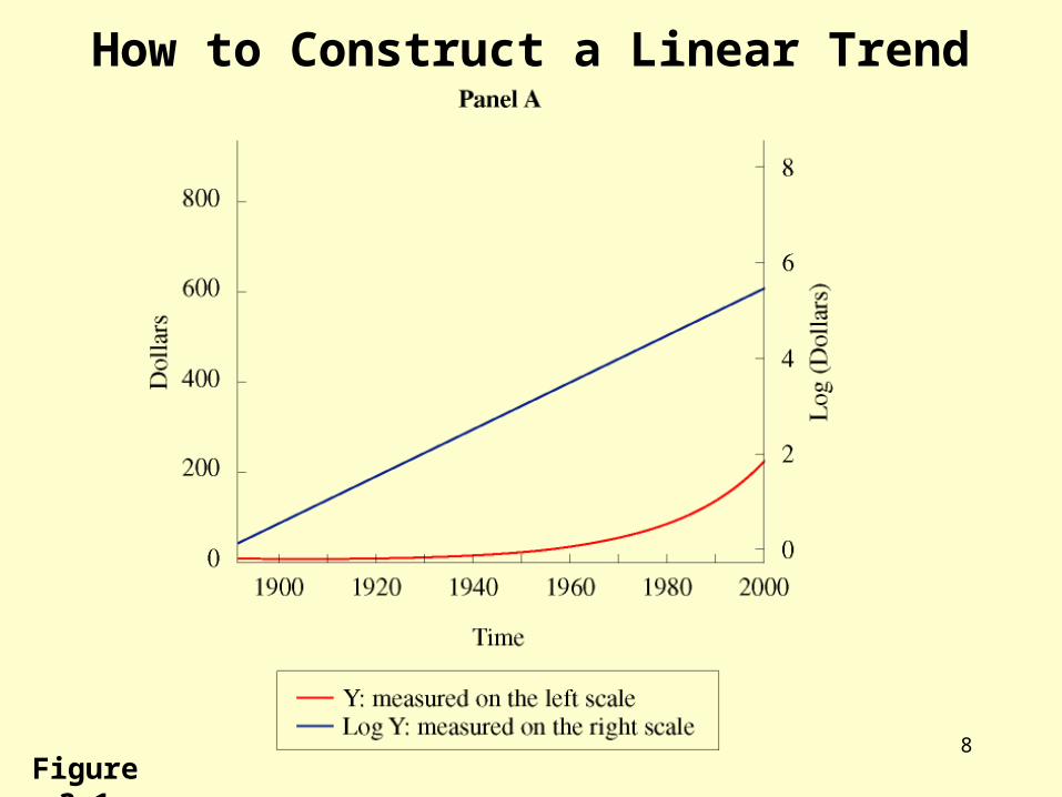
8Figure 3.1
How to Construct a Linear Trend

9
Transforming Economic Data
• Removing a Trend- Many economics variables have an underlying
growth rate that is constant, but it fluctuate randomly around this underlying rate from one year to the next.
- Linear detrending is to fit the best straight line through the graph of the logarithm.
- The fitted line is called the linear trend (low-frequency) and the deviations from the fitted line are called the linear cycle (high-frequency).

10Figure 3.1
How to Construct a Linear Trend
11
Transforming Economic Data
• Detrending Method
- The linear trend has the disadvantage that the trend itself is assumed constant.
- If a series is detrended using the linear method, the series may deviate from its underlying growth rate in the long run. we need to fit a flexible trend.

12
Transforming Economic Data
• Detrending Method
- A third method of revealing the high-frequency relationship is to look at a growth rates of data rather than at the raw data itself
differencing
1987 19861987
1986
GDP GDPDGDP
GDP

13
Transforming Economic Data
• Importance of Detrending
- Detrending reveals relationships between time series that exist at on frequency but not at another.
- Many relationship can be easily observed from the high-frequency component.
- See Figure 3.2
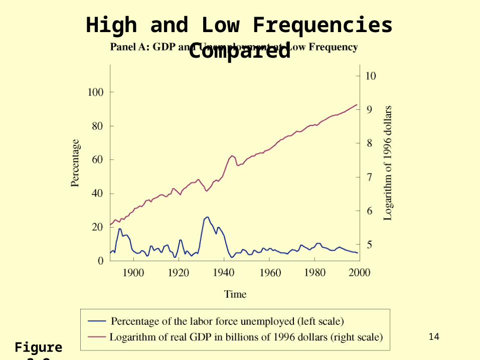
14Figure 3.2
High and Low Frequencies Compared
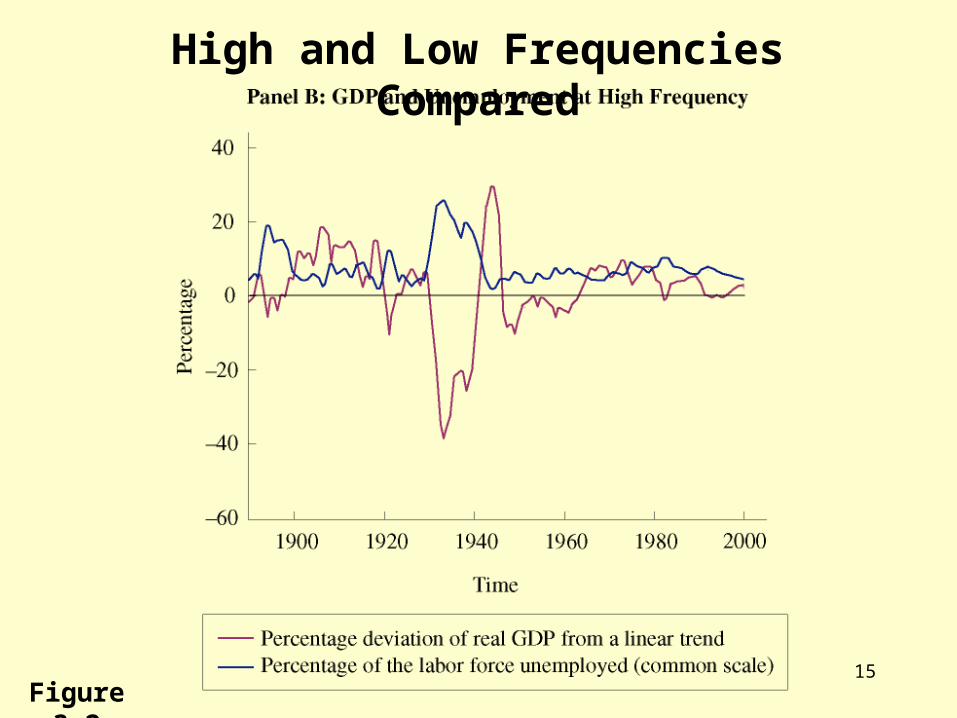
15Figure 3.2
High and Low Frequencies Compared

16
Transforming Economic Data
• Quantifying Business Cycles
- The business cycle is an irregular, persistent fluctuation of real GDP around its trend growth rate.
- It is accompanies by highly coherent co-movements in many other economic variables.

17
Transforming Economic Data
• Quantifying Business Cycles
- One tool used to describe business cycles is the correlation coefficient.
- It is used to measure the strength of a relationship between two variables (coherence) and the strength of the relationship between a single variable and its own history (persistence).

18
Transforming Economic Data
• Peaks and Troughs- The common features of business cycles are
peaks, troughs, expansions and recessions. Ex: GDP- Peak: the point at which the growth rate of
GDP begins to decline.- Trough- Expansion: the period between a trough and its
subsequent peak.- Recession

19©2002 South-Western College PublishingFigure 3.3
A Stylized Business Cycle

20
Transforming Economic Data
• Peaks and Troughs
- Real data do not display the kinds of regularities as in figure 3.3.
- The regularities in economic data are statistical.
- No two business cycles are exactly alike, so we aim at their average behavior and relationship.

21
Transforming Economic Data
• The Correlation Coefficient
- Scatter Plot : a graph in which each each point represents an observation from two different variables at a given time. (See Figure 3.4)
- Statistician have developed a way of quantifying the relationship between two variables in a scatter plot with a single number the correlation coefficient.

22
Transforming Economic Data
• The Correlation Coefficient
1
2 2
n
i ii
xy
i i
xy
x y
x x y y
x x y y
23
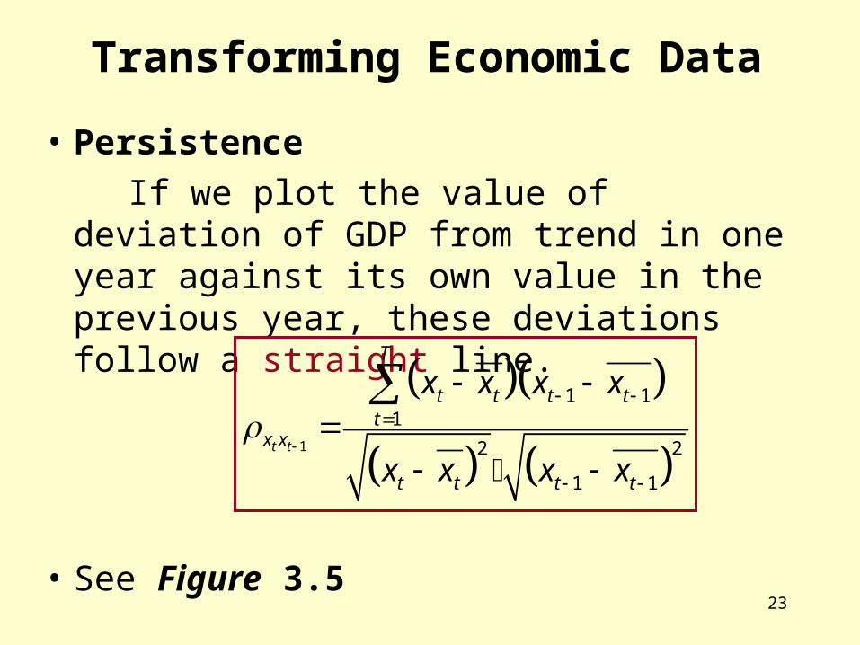
Transforming Economic Data
• Persistence
If we plot the value of deviation of GDP from trend in one year against its own value in the previous year, these deviations follow a straight line.
• See Figure 3.5
1
1 11
2 2
1 1
t t
T
t t t tt
x x
t t t t
x x x x
x x x x

24
Transforming Economic Data
• Coherence
- A second important feature of economic time series is that they tend to move together coherence.
1
2 2
T
t tt
xy
t t
x x y y
x x y y

25
Transforming Economic Data
• Coherence
- If a time series goes up (down) when GDP goes up (down), we say the series is procyclical.
ex. Consumption, Investment
- A series that moves in the opposite direction to GDP is countercyclical.
ex. Unemployment
- See BOX 3.1

26Table 3.1
27
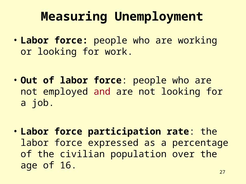
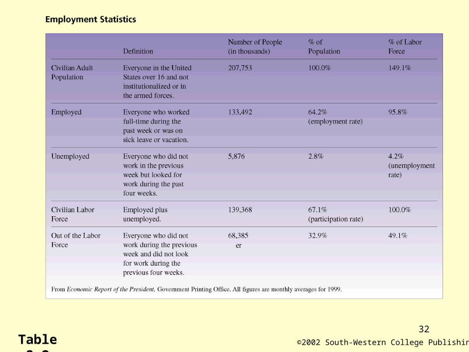
Measuring Unemployment
• Labor force: people who are working or looking for work.
• Out of labor force: people who are not employed and are not looking for a job.
• Labor force participation rate: the labor force expressed as a percentage of the civilian population over the age of 16.

28
Measuring Unemployment
• Employment Rate:
the fraction of the population employed.
• Unemployment Rate:
the fraction of the labor force looking for a job.
employed
adult population
unemployed
labor force

29Box 3.2A
Labor Force Participation Since 1950

30Box 3.2B
Labor Force Participation Since 1950

31
Measuring Unemployment
• Does a increase in the employment rate imply a decrease in the unemployment rate ?
employedemployment rate =
adult population
employed
labor force + out of labor force
unemployedunemployment rate =
labor force
32
©2002 South-Western College PublishingTable 3.2

33
Measuring GDP Growth
- Real GDP was measured by the base-year method.
- Recently, the Commerce Department has switched to the chain weighted method as an alternative to reduce the relative price effects.

34

35
From GDP Growth to GDP
Index of real GDP and the chain weighting method.
36
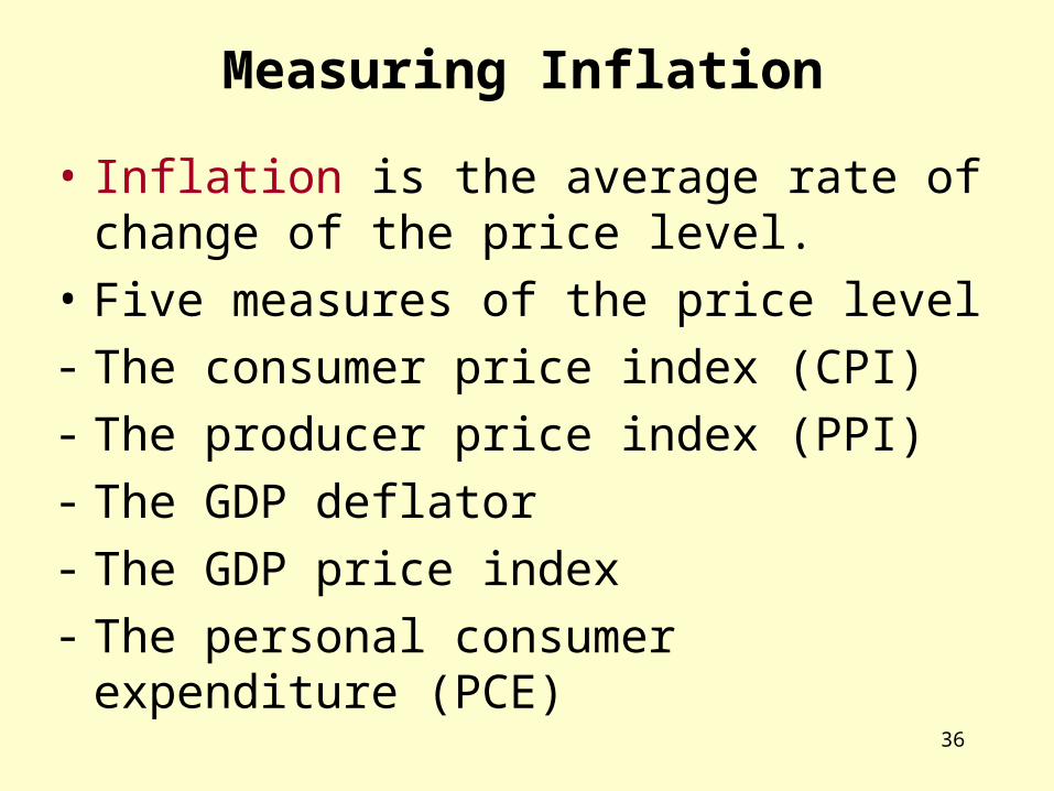
Measuring Inflation
• Inflation is the average rate of change of the price level.
• Five measures of the price level
- The consumer price index (CPI)
- The producer price index (PPI)
- The GDP deflator
- The GDP price index
- The personal consumer expenditure (PCE)
37
Measuring Inflation
• A price index is a weight average of the prices of many different commodities where weights are constants that are multiplied by each price and that sum to one.
• The weights denotes importance.

38
Different Kinds of Price Indices
• Three alternative kinds of price indices:
- Laspeyres (CPI, PPI GDP deflator)
past consumed bundle
- Paasche (GDP deflator)
current consumed bundle
- Superlative (GDP price index, PCE)

39
The CPI and the PPI
• CPI tried to measure the average cost of living of a representative household.
• PPI tried to measure the average cost of the inputs of a representative producer.
• Many economists watch the PPI closely since price increases that occur in the PPI often eventually end up in the CPI
PPI is the leading indicator of inflation.
• Shortage: It overstates inflation. (Laspeyres)
40
The GDP Deflator and the GDP Price Index
• Corresponding to the Commerce Department’s switch from a base-year to a chain weighted measure of growth, there has been a switch from the GDP deflator to the GDP price index.
• Example: Table 3.3, 1999-2000
• For GDP price indices, inflation is measured as the average of the percentage change in the price indices obtained from using adjacent years as the base.

41
The PCE Price Index
• Like the GDP price index, PCE is a Superlative index.
• Like the CPI, the PCE includes only those commodities that represent personal consumption expenditures by households.

42
Inflation and the Business Cycle
• Many time series are strongly procyclical (e.g., consumption) or strongly countercyclical (e.g., unemployment).
• Inflation is neither procyclical nor countercyclical.
See Figure 3.6.

43
Inflation and the Business Cycle
• Figure 3.7• 1920-40 : Inflation seems to be procyclical.• 1940-90: Inflation seems to be countercyclical.• Keynes believed that the Great Depression was
caused by the demand shocks and inflation would be procyclical.
• Real business cycle theorists assert that most business fluctuations occur as a result of changes in productivity, and they predict that inflation should be countercyclical.

44©2002 South-Western College PublishingFigure 3.7
Growth and Inflation: Pre- and Postwar

45
Homework
Question 4, 6, 7, 12, 13

END