Macroeconomic factors and micro-level bank risk

Claudia M. Buch(University of Tübingen, CESifo and IAW)

Sandra Eickmeier(Deutsche Bundesbank)

Esteban Prieto(University of Tübingen)

Discussion PaperSeries 1: Economic StudiesNo 20/2010Discussion Papers represent the authors’ personal opinions and do not necessarily reflect the views of theDeutsche Bundesbank or its staff.

Editorial Board: Klaus Düllmann Frank Heid Heinz Herrmann Karl-Heinz Tödter Deutsche Bundesbank, Wilhelm-Epstein-Straße 14, 60431 Frankfurt am Main, Postfach 10 06 02, 60006 Frankfurt am Main Tel +49 69 9566-0 Telex within Germany 41227, telex from abroad 414431 Please address all orders in writing to: Deutsche Bundesbank, Press and Public Relations Division, at the above address or via fax +49 69 9566-3077

Internet http://www.bundesbank.de

Reproduction permitted only if source is stated.

ISBN 978-3–86558–650–6 (Printversion) ISBN 978-3–86558–651–3 (Internetversion)

Abstract

The interplay between banks and the macroeconomy is of key importance for financial and economic stability. We analyze this link using a factor-augmented vector autoregressive model (FAVAR) which extends a standard VAR for the U.S. macroeconomy. The model includes GDP growth, inflation, the Federal Funds rate, house price inflation, and a set of factors summarizing conditions in the banking sector. We use data of more than 1,500 commercial banks from the U.S. call reports to address the following questions. How are macroeconomic shocks transmitted to bank risk and other banking variables? What are the sources of bank heterogeneity, and what explains differences in individual banks’ responses to macroeconomic shocks? Our paper has two main findings: (i) Average bank risk declines, and average bank lending increases following expansionary shocks. (ii) The heterogeneity of banks is characterized by idiosyncratic shocks and the asymmetric transmission of common shocks. Risk of about 1/3 of all banks rises in response to a monetary loosening. The lending response of small, illiquid, and domestic banks is relatively large, and risk of banks with a low degree of capitalization and a high exposure to real estate loans decreases relatively strongly after expansionary monetary policy shocks. Also, lending of larger banks increases less while risk of riskier and domestic banks reacts more in response to house price shocks.

JEL codes: E44, G21

Keywords: FAVAR, bank risk, macro-finance linkages, monetary policy, microeconomic adjustment

Non-technical summary

The interplay between banks and the macroeconomy is of key importance for financial and economic stability. We analyze this link using a factor-augmented vector autoregressive model (FAVAR) which extends a standard VAR for the US macroeconomy over the period 1985-2008. The model includes GDP growth, inflation, the Federal Funds rate, house price inflation, and a set of factors summarizing conditions in the banking sector (not interpreted further). We use data of more than 1,500 commercial banks from the US Call Reports. We make several contributions to the existing literature. First, the FAVAR model allows us to analyze the dynamic interactions between bank-specific and macroeconomic developments in a flexible way while taking into account the endogeneity of macro factors and banking factors. Second, the model permits the inclusion of a large set of bank-level information and therefore to model linkages between individual banks and between different banking variables. Moreover, we can assess the exposure of each individual bank to macroeconomic shocks. Third, previous papers analyzing the bank lending channel or the risk-taking channel regress bank-level loans or risk on the monetary policy interest rate, GDP growth, or asset prices which are, in general, driven by a number of different shocks while we focus on the impact of identified orthogonal shocks on bank variables. Fourth, FAVAR models have previously mostly been fitted to large macroeconomic or aggregate financial datasets, while we fit our FAVAR to micro-level data.

We address the following questions.

(i) What is the effect of macroeconomic shocks on bank risk, capitalization, returns, and lending?

(ii) What explains the heterogeneous reactions to these and other disturbances across banks? How important are idiosyncratic shocks vs. the asymmetric transmission of common shocks? Which bank-level features affect the exposure of banks to monetary policy and house price shocks?

We find that average bank risk declines, and average bank lending increases, following expansionary shocks. Shocks to banking factors matter for economic activity, especially in the medium term, when they explain more than 25 percent. Their explanatory power is even larger for house prices and the monetary policy interest rate (over 30 percent). The heterogeneity of banks is characterized by both idiosyncratic shocks and the asymmetric transmission of common shocks. While average risk declines, risk of about 1/3 of all banks rises in response to a monetary loosening. Lending of small, not very liquid, and domestic banks increases and risk of banks with a low degree of capitalization and a large fraction of real estate loans in total loans decreases relatively strongly after expansionary monetary policy shocks. Also, lending of larger banks increases less while risk of riskier and domestic banks responds more to house price shocks.

Nicht-technische Zusammenfassung

Wie Banken und die Makroökonomie zusammen wirken, ist für eine Volkswirtschaft sehr wichtig, nicht zuletzt auch für die Stabilität des Finanzsystems. Das vorliegende Papier analysiert diesen Zusammenhang für die USA mit Hilfe eines ‘factor-augmented vector autoregressive model (FAVAR)’, welches ein Standard-VAR über den Zeitraum 1985-2008 erweitert. Wir modellieren den Zuwachs des Bruttoinlandsprodukts, die allgemeine Inflation, den Notenbankzins, die Inflation der Immobilienpreise zusammen mit einer Reihe von Faktoren, welche die Entwicklungen im Bankensystem zusammenfassen (die aber nicht näher interpretiert werden). Dazu verwenden wir Daten von über 1500 Geschäftsbanken aus den US Call Reports. Das Papier leistet in vierfacher Hinsicht einen Beitrag, der über die bereits existierende Literatur hinausgeht. Erstens lassen sich mit Hilfe des FAVARs die dynamischen Interaktionen zwischen bankspezifischen und makroökonomischen Entwicklungen in flexibler Weise modellieren. Makro- und Bankenfaktoren können sich dabei gegenseitig beeinflussen. Zweitens kann eine Vielzahl von Daten auf der Ebene einzelner Banken einbezogen werden. Insofern können die Verflechtungen zwischen einzelnen Banken und zwischen unterschiedlichen Bankenvariablen modelliert werden. Des Weiteren können wir die Effekte makroökonomischer Schocks auf einzelne Banken abschätzen. Drittens untersuchen wir die Übertragung identifizierter orthogonaler Schocks auf Banken, während vorangegangene Analysen die Kreditvergabe beziehungsweise das Risiko einzelner Banken auf den geldpolitischen Zins, den Zuwachs des Bruttoinlandsprodukts oder die Vermögenspreisinflation, die in der Regel von einer Reihe unterschiedlicher Schocks getrieben werden, regressiert haben. Viertens wurden FAVAR-Modelle zuvor vor allem auf große makroökonomische oder aggregierte Finanzmarktdatensätze angewandt, während wir unser FAVAR auf einen Mikro-Datensatz anwenden.

Die folgenden Fragen werden beantwortet.

(i) Wie beeinflussen makroökonomische Schocks das Risiko sowie die Kapitalisierung, den Ertrag und die Kreditvergabe von Banken?

(ii) Was erklärt die Heterogenität, mit der Banken auf solche und andere Störungen reagieren? Wie wichtig sind idiosynkratische (bank-spezifische) Schocks im Vergleich zur asymmetrischen Übertragung gemeinsamer Schocks? Welche bankspezifischen Eigenschaften sind Ausschlag gebend für die Reaktion von Banken nach geldpolitischen und Immobilienpreisschocks?

Wir finden einen Rückgang des durchschnittlichen Bankenrisikos und einen Anstieg der durchschnittlichen Kreditvergabe nach expansiven Schocks. Schocks auf die Bankenfaktoren sind für die gesamtwirtschaftliche Entwicklung nicht unerheblich, vor allem in der mittleren Frist, in der sie über 25 Prozent erklären. Ihr Erklärungsgehalt ist besonders groß für die Entwicklung der Immobilienpreise und des geldpolitischen Zinses (über 30 Prozent). Heterogenität in den Entwicklungen von Banken ergibt sich sowohl aufgrund idiosynkratischer Schocks als auch der asymmetrischen Übertragung gemeinsamer Schocks. Zwar sinkt das durchschnittliche Bankenrisiko, das Risiko von einem Drittel aller untersuchten Banken allerdings steigt nach einem expansiven geldpolitischen Schock. Die Kreditvergabe kleiner, nicht besonders liquider und Banken, deren Geschäft auf das Inland

begrenzt ist, erhöht sich und das Risiko von Banken mit einer niedrigen durchschnittlichen Eigenkapitalquote und einem großen Anteil von Immobilienkrediten an den Krediten insgesamt verringert sich relativ stark nach expansiven geldpolitischen Schocks. Wir finden zudem, dass die Kreditvergabe relativ risikoreicher Banken ohne oder geringem internationalem Geschäft nach positiven Immobilienpreisschocks in geringerem Maße steigt, während ihr Risiko stärker sinkt.

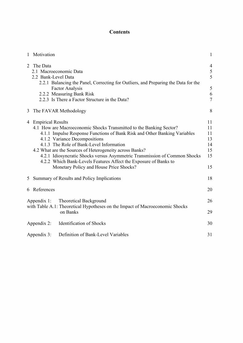
Contents 1 Motivation 1 2 The Data 4 2.1 Macroeconomic Data 5 2.2 Bank-Level Data 5 2.2.1 Balancing the Panel, Correcting for Outliers, and Preparing the Data for the Factor Analysis 5 2.2.2 Measuring Bank Risk 6 2.2.3 Is There a Factor Structure in the Data? 7 3 The FAVAR Methodology 8 4 Empirical Results 11 4.1 How are Macroeconomic Shocks Transmitted to the Banking Sector? 11 4.1.1 Impulse Response Functions of Bank Risk and Other Banking Variables 11 4.1.2 Variance Decompositions 13 4.1.3 The Role of Bank-Level Information 14 4.2 What are the Sources of Heterogeneity across Banks? 15 4.2.1 Idiosyncratic Shocks versus Asymmetric Transmission of Common Shocks 15 4.2.2 Which Bank-Levels Features Affect the Exposure of Banks to Monetary Policy and House Price Shocks? 15 5 Summary of Results and Policy Implications 18 6 References 20 Appendix 1: Theoretical Background 26 with Table A.1: Theoretical Hypotheses on the Impact of Macroeconomic Shocks on Banks 29 Appendix 2: Identification of Shocks 30 Appendix 3: Definition of Bank-Level Variables 31

Table and Figures Table 1: Correlation Between Median Banking Variables 32 Table 2: Cumulated Variance Shares Explained by the First 15 Principal Components Calculated from Datasets Associated with Individual Banking Variables 32 Table 3: Identifying Restrictions 33 Table 4: Forecast Error Variance Decomposition 33 Table 5: Dispersion of Common and Idiosyncratic Components 33 Table 6: Regression Results 34 Figure 1: Kernel Densities of Banking Variables – Balanced versus Unbalanced Data 35 Figure 2: Comparison of Bank Risk Measures 36 Figure 3: Impulse Response Functions of Macroeconomic Factors 37 Figure 4: Impulse Response Functions of Median Banking Variables 38 Figure 5: Impulse Response Functions of Macroeconomic Factors from the Baseline FAVAR and a VAR without Micro-Level Information 39 Figure 6: Monetary Policy Shock Series 40 Figure 7: Impulse Response Functions of Individual Banks (5th to 95th Quantiles) 41

1 Motivation

How are macroeconomic shocks transmitted to bank risk and other banking variables? What are the sources of bank heterogeneity, and what explains differences in individual banks’ responses to macroeconomic shocks? We provide answers to these questions by analyzing the exposure of banks to macroeconomic developments in the U.S. over the period 1985-2008.

Our analysis is based on a factor-augmented vector autoregressive model (FAVAR) in the tradition of Bernanke et al. (2005) which extends a standard macroeconomic VAR comprising GDP growth, inflation, house price inflation, and the monetary policy interest rate with a set of factors summarizing a large amount of information from bank-level data. Our bank-level dataset contains bank risk which is our focus. We also include bank capitalization, profitability, and loans as bank-level variables which affect the transmission mechanism of macroeconomics shocks on risk. Data for a balanced panel of about 1,500 banks are taken from the U.S. call reports. We decompose the banking data into common and idiosyncratic components. A set of macroeconomic (supply, demand, monetary policy and house price) shocks is identified and, based on an impulse response analysis, their transmission through the banking system is assessed. We look at the effects of the shocks not only on aggregate bank variables, but we also on individual banks. Using cross-sectional regressions, we study which bank-level features can explain differences in banks’ responses to macroeconomic shocks.

Our main findings are as follows. (i) Average bank lending increases following expansionary shocks. Average bank risk declines after most expansionary macroeconomic shocks. House price and monetary policy shocks are particularly important for bank risk. (ii) There is a substantial degree of heterogeneity across banks both in terms of idiosyncratic shocks and the asymmetric transmission of common (banking and macroeconomic) shocks. While average risk declines, risk of a sizeable fraction of banks rises in response to expansionary shocks. The degree of capitalization, the exposure to real estate loans, the riskiness and the presence of foreign affiliates matter for individual banks’ risk responses.

Corresponding author: Sandra Eickmeier, Deutsche Bundesbank, Economic Research Centre, Wilhelm-Epstein-Str. 14, 60431 Frankfurt am Main, Germany, Phone: +49 69 9566 4705. E-mail: sandra.eickmeier@bundesbank.de. The views expressed in this paper do not necessarily reflect the views of the Deutsche Bundesbank. The paper has partly been written during visits of C.M. Buch and E. Prieto to the research centre of the Deutsche Bundesbank. The hospitality of Bundesbank is gratefully acknowledged. We would like to thank Falko Fecht, Heinz Herrmann, Thomas Laubach as well as the participants of the Annual Meeting of the Monetary Group of the Verein für Socialpolitik, held in Gerzensee in February 2010, at the CESifo Conference on Macro, Money, and International Finance (Munich, Februar 2010), at a seminar at the Bundesbank, at the 16th International Conference on Computing in Economics and Finance (London, July 2010) and the Annual Conference of the Verein für Socialpolitik (Kiel, September 2010) for most helpful comments on an earlier version of this paper. All errors and inconsistencies are solely in our own responsibility.

1

Our study is related to theoretical and empirical work on the effects of macroeconomic (mostly monetary policy) developments on bank risk. Financial accelerator mechanisms imply that changes in interest rates may have countervailing effects on bank risk. On the one hand, lower interest rates reduce the interest rate burden for firms, lower the risk of outstanding flexible loan contracts, thereby increasing the probability of repayment and the value of the underlying collateral. On the other hand, the borrowing capacity of high-risk firms increases with the value of pledgeable assets. Also, banks might engage in riskier, high yield, projects to offset the negative effects of lower interest rates on profits. Risk might increase. Conversely, higher interest rates increase the agency costs of lending, banks reduce the amount of credit to monitoring-intensive firms, and they invest more in safe assets (“flight-to-quality”) (Bernanke et al. 1996, Dell’Ariccia and Marquez 2006, Matsuyama 2007).

While the original financial accelerator models do not assign a specific role to banks, recent macroeconomic models explicitly analyze the feedback between banks and the macroeconomy in the context of dynamic stochastic general equilibrium (DSGE) models (Angeloni and Faia 2009, Dib 2010, Gerali et al. 2010, Meh and Moran 2010, Zhang 2009).1 In these models, the impact of expansionary shocks on bank lending is unequivocally positive, but the impact on bank risk is less clear cut (Appendix 1 and Table A.1). In Angeloni and Faia (2009), for instance, a declining interest rate, following a positive supply or monetary policy shock, reduces banks’ funding costs and increases the probability to repay depositors. To maximize profits, banks optimally choose to increase leverage. But the decline in interest rates also lowers banks’ return on assets and this, together with higher leverage, increases bank risk. In Zhang (2009), on the contrary, expectations of future outcomes play a central role. A positive technology shock, for instance, increases the return on capital above its expected value which in turn corresponds to a lower than expected loan default rate. The bank thus realizes unexpected profits on its loan portfolio. Bank capital is accumulated through these earnings, strengthening banks’ balance sheet positions and reducing risk.

A small set of empirical papers looks at the impact of monetary policy shocks on bank risk, with ambiguous findings. A few recent papers analyze the risk-taking channel of monetary policy and investigate whether low policy interest rates encourage lending to high-risk borrowers (Rajan 2005, Borio and Zhu 2008). Empirical studies based on bank-level data find evidence that lower interest rates increase bank risk (Altunbas et al. 2009, Gambacorta 2009, Ioannidou et al. 2009, Jiménez et al. 2007).2 Based on time series evidence for the U.S.,

1 These models differ with regard to the financial frictions (demand- versus supply-side), the assumptions on the degree of competition in the banking sector, the modeling of bank risk, the stickiness of interest rates, and the types of macroeconomic shocks. 2 The risk-taking channel focuses on the incentives to engage in ex ante riskier projects. We instead measure changes in bank risk ex post. Our data do not allow isolating changes in the structure of the existing portfolios of banks and the structure of new lending (Jiménez et al. 2007). Also, we do not control for the duration of a

2

Eickmeier and Hofmann (2010) and Angeloni et al. (2010) find a decline of various credit risk spreads and an increase of bank balance sheet risk, respectively, following a positive monetary policy shock. Using a model that captures the feedback between bank-level distress and the macroeconomy, De Graeve et al. (2008), in contrast, find a decline in German banks’ probability of distress after a monetary policy loosening. The impact of other shocks has, to the best of our knowledge, so far not been subject to careful empirical investigation.3

Our modeling approach implicitly accounts for the key mechanisms stressed in the theoretical papers and provides empirical evidence on the net effect of macroeconomic shocks on bank risk.

Our main research question, the exposure of banks to macroeconomic factors, also features prominently in recent proposals for regulatory reforms (Basel Committee 2009). Rochet (2008) suggests on the basis of a theoretical model that banks should face a capital requirement and a deposit insurance premium that increases with their exposure to macroeconomic factors. Farhi and Tirole (2009) analyze the incentives of banks to coordinate their exposure to macroeconomic shocks, and they argue that banks which react more to macroeconomic factors should be regulated more tightly. Gersbach and Hahn (2009) propose a regulatory framework under which a banks’ required level of equity capital depends on the equity capital of its peers and, in this sense, on the macroeconomic environment. Implementing these proposals requires information about individual banks’ exposures to macroeconomic factors. Our results inform this debate.

We make several contributions. First, the FAVAR model allows analyzing the dynamic interaction between bank-specific and macroeconomic developments in a flexible way. Several VAR-studies allow for the interaction between credit and macroeconomic factors (e.g. Ciccarelli et al. 2009, Eickmeier et al. 2009), but these studies do not focus on bank risk or bank-specific effects. Bank-level studies on the risk-taking or bank lending channel, in contrast, allow macroeconomic factors to affect bank risk, but macroeconomic factors are not modeled as a function of banking variables. Our setup accounts for the endogeneity of both, macroeconomic- and banking factors.

Second, the FAVAR allows including lots of bank-level data. The factor model exploits the comovement between individual banks and allows us to model linkages between individual banks, i.e. through the interbank market or the exposure to common shocks. The need to account for linkages between financial institutions is one key lesson of the recent crisis

particular monetary policy stance but consider “average” shocks over the entire sample period (Altunbas et al. 2009). For these reasons, our results are not directly comparable with results for the risk-taking channel of monetary policy. 3 Altunbas et al. (2009) find that higher GDP growth lowers bank risk but changes in asset prices have no clear-cut impact in risk. The analysis of these factors in risk is, however, not the focus of their paper. Moreover, the authors do not identify structural (real or asset price) shocks.

3

(Brunnermeier 2008, IMF 2009). Moreover, we model the interaction between different banking variables, including the risk and the return of banks, and thus accounting for the fact that, in “search for yield”, banks may increase risk (Hellwig 2008, Rajan 2005). Another important implication of the fact that we can include lots of bank-level data in our model is that we can assess the exposure of each individual bank to macroeconomic shocks.

Third, previous papers analyzing the bank lending channel or the risk-taking channel regress bank-level lending or risk on the monetary policy interest rate, GDP growth, or asset prices (e.g. Altunbas et al. 2009, Cetorelli and Goldberg 2008, Ioannidou et al. 2009, Jiménez et al. 2007, Kashyap and Stein 2000).4 The macroeconomic indicators are reduced-form constructs, and their developments may reflect the pass-through of different types of shocks. Instead, we consider identified orthogonal macroeconomic shocks which allow us to better disentangle the common drivers of banking developments.

Fourth, FAVAR models have previously been fitted to large macroeconomic datasets (e.g. Bernanke et al. 2005, Boivin and Giannoni 2008) or aggregate financial datasets (e.g. De Nicoló and Lucchetta 2010, Eickmeier and Hofmann 2010). The methodology, however, allows exploiting even richer information, and its application also to micro-level data is the natural next step. We will show that omitting bank-level information might bias estimates of impulse responses and shocks series. Our study is one of the first using a FAVAR model linked to a micro-level dataset. It is closely related to Dave et al. (2009) who use a similar modeling approach for U.S. data but focus on the bank lending channel while our focus is on risk.5

In Sections 2 and 3, we present the data and the FAVAR methodology, respectively. In Section 4, we provide and discuss the empirical results and conclude in Section 5.

2 The Data

The key feature of our empirical model is the joint analysis of macroeconomic data and bank-level data, which we describe in this section. We also compare our risk measure to alternative risk measures used in the literature and address potential concerns regarding the presence of a factor structure in the data.

4 These papers on risk-taking address the issue that monetary policy is endogenous by either approximating monetary policy of the countries studied by foreign policy rates (Jiménez et al. 2007) or by Taylor rule gaps, i.e. deviations of the policy rate from the rate implied by the Taylor rule (Altunbas et al. 2009). 5 Other papers combining factor models and micro-level data (with a different focus) are Den Reijer (2007) and Otrok and Pourpourides (2008).

4

2.1 Macroeconomic Data

Our set of macroeconomic variables comprises log differences of real GDP, the GDP deflator, real house prices, and the level of the effective Federal Funds rate. Real house prices are measured as the Freddie Mac Conventional Mortgage house price, divided by the GDP deflator. The data are retrieved from FreeLunch.com, a free internet service provided by Moody’s Economy.com.

2.2 Bank-Level Data

Our source for bank-level data is the Consolidated Report of Condition and Income (call reports) that all insured commercial banks in the United States submit to the Federal Reserve each quarter. A complete description of all variables is provided in Appendix 3. From the call reports, we compile a dataset consisting of quarterly income statements and balance sheet data over the period 1985Q1–2008Q2, i.e. our analysis does not include the period following the bankruptcy of Lehman Brothers. (See Frankel and Saravelos (2010) for a similar definition of the pre-crisis period.) Using instead information up to the beginning of the Great Recession in the fourth quarter of 2007 does not qualitatively change our main results.

We consider the following banking variables. Bank risk is measured using the share of non-performing loans in total loans. The (unweighted) ratio of equity capital to total assets is used as a measure of bank balance sheet strength. Our measure of banks’ profitability is return on assets, defined as net income to total assets. Finally, we include (growth of) total bank loans.

2.2.1 Balancing the Panel, Correcting for Outliers, and Preparing the Data for the Factor Analysis

Following previous micro banking studies, we apply a number of screens to exclude implausible and unreliable observations. We exclude observations with (i) negative or missing values for total assets, (ii) negative total loans, (iii) loan-to-assets ratios larger than one, or (iv) capital-to-assets ratios larger than one. In addition, entire banks with gross total assets below $25 million and banks engaged in a merger are dropped from the sample.6 Finally, if one of the three ratios (non-performing loans-to-total loans, capital-to-assets, and net income-to-assets) of an individual bank falls in the bottom or top percentile at any point in time, the entire bank is dropped. We only include banks which are in business during the entire period under study. Overall, these corrections reduce the sample from 13,375 banks in the unbalanced panel to 1,512 banks in the balanced panel. Figure 1 shows that balancing has not much changed the distribution of the data.

6 Berger and Bouwmann (2009) state that banks with total assets below $25 millions are not likely to be viable commercial banks.

5

The bank-level data are treated in the usual manner for factor analysis. All series are seasonally adjusted, and they enter the dataset as stationary variables. Because loans are assumed to be integrated of order 1, we include them as log differences in our model. The balance sheet ratios can be considered stationary, hence there is no need to difference them. The stationary series are then demeaned, and structural breaks in the means are accounted for.7 Moreover, the series are standardized to have unit variance, and outliers are removed. Outliers are defined as observations with absolute median deviations larger than six times the interquartile range. They are replaced by the median value of the preceding five observations (Stock and Watson 2005).

2.2.2 Measuring Bank Risk

The non-performing loans ratio is our main measure of bank risk. It captures the asset risk of banks and thus the share of bank loans that are actually in default. This measure is available for a large number of banks for a long time period. Another advantage is that it is not much affected by changes in accounting standards. Also, it matches up with theoretical models that describe banks as intermediaries between depositor and lenders and that consider loan defaults as the main source of instabilities in banking (e.g. Boyd and De Nicoló 2005, Martínez-Miera and Repullo 2010, Zhang 2009).

Alternative measures of bank risk have been used in the literature as well (see, e.g. Beck 2008 for a survey), and Figure 2 shows how they are related to the non-performing loans ratio. The z-score measure is calculated using information on banks’ level of equity, the standard deviation of profits, and profits. Loosely speaking, the z-score is inversely related to the probability that the bank’s equity base is eroded, e.g. higher values indicate less risk. Although the focus of this risk measure differs from the non-performing loans ratio, the z-score for the U.S. banking system tracks the median non-performing loans ratio quite well (Figure 2a). The disadvantage of the z-score is that it requires calculating the volatility of profits over a certain time window, the choice of which is somewhat arbitrary.8 Figure 2a also reveals that the non-performing loans ratio is highly correlated with the cross-section dispersion of individual banks’ return on assets. This measure is the banks’ counterpart of the cross-section dispersion of firms’ earnings which has been used in the literature to capture uncertainty or risk in the business sector (as, e.g., discussed in Bloom 2009).

7 Some ratios do not seem to revert to a constant mean. This is possibly due to regulatory changes which led to an adjustment in capital ratios and other banking variables. To account for these changes, we detect breakpoints by applying the sequential multiple breakpoint test of Bai and Perron (1998, 2003) (and the Gauss routines provided by Pierre Perron on his webpage) to all series of our (stationary) dataset, and we subtract the (possibly shifted) means from the series (see Eickmeier 2009 for a similar treatment of (macroeconomic) data in a factor modelling setup). When we, instead, linearly detrend the series, the results are basically unaffected. 8 Related to this, the z-score, as it is shown in Figure 2, by construction, lags the non-performing loans ratio.

6

Finally, we have checked how more market-based measures of bank risk are related with the median non-performing loans ratio (see Figure 2b). We have used CDS spreads obtained from Bloomberg, EDFs from Moody’s KMV, and stock market volatility (source: Goldman Sachs).9 One disadvantage of these measures is that they are not available for the full sample period or for all banks. CDS spreads and EDFs trace the non-performing loans ratio reasonably well. These market-based measures, however, tend to peak in times of financial market stress. The non-performing loans ratio, in contrast, shows a much smoother pattern and arguably tracks fundamental risk of banks in a more reliable way.

2.2.3 Is There a Factor Structure in the Data?

Exploiting a rich amount of (bank-level) information can be beneficial in a factor analysis. Our factor model, however, also needs to provide a good description of the data. For this to be the case, there needs to be a factor structure among the series included, or, put differently, factors can be accurately estimated only if the series strongly co-move (Boivin and Ng 2006). This issue is particularly relevant for microeconomic data as opposed to (aggregate) macroeconomic data to which factor models have been previously employed and which tend to exhibit a greater comovement.

We first assess to what extent the different banking variables (risk, capitalization, return, lending) are correlated. Table 1 shows that the medians are highly correlated. The non-performing loans ratio and capitalization are particularly strongly (negatively) correlated because a decline in asset quality forces banks to write down assets. The correlation is, however, not perfect. Unlike the non-performing loans ratio, capitalization is also determined by regulatory requirements. Moreover, banks use it as a signaling devise and might avoid adjustments in response to negative macroeconomic shocks.

We next examine to what extent individual banks are related. Table 2 shows the variance shares explained by the first 15 principal components extracted separately from bank-level datasets associated with each of the four variables. There is reasonably strong comovement among banks for all banking variables with 6 factors explaining at least 40 percent and 9 factors explaining at least 50 percent of the variation in the ratios. The comovement is a bit lower for loan growth where 7 and 12 factors are needed to explain 40 and 50 percent, respectively.

We have carried out further robustness checks. We have first removed cross-sectional outliers from the dataset, i.e. we have dropped banks from the sample with absolute median deviations larger than six times the interquartile range (on average over the sample period).10 We have also downweighted each bank-level series by the inverse of the standard deviation

9 We thank Yener Altunbas and David Marqués Ibañez for their help with the EDF series. 10 This procedure identifies about 300 series as outliers.

7

of its idiosyncratic component (weighted principal components, see Boivin and Ng 2006). Finally, we have aggregated the balance sheets of all banks that belong to the same bank holding company. This alternative dataset contains 560 bank holding companies, and we have extracted factors from this dataset. Bank holding companies may be able to shift resources among the banks they control (Kashap and Stein 2000), and we would expect the comovement between bank holding companies to be larger than between individual banks. The factors extracted from our original dataset and the factors estimated in these robustness checks are very highly correlated. The trace R² from a regression of the principal components extracted from the original dataset on the principal components estimated from the modified datasets lie between 0.95 and 0.99.11

As a final check, we have assessed whether omission of regional banking factors affect our estimation of the national factors. We have separately extracted factors from the bank-level data by state using principal components. We have then pooled the state-level factors and estimated national factors from the pooled dataset (see, e.g., Del Negro and Otrok 2007, Kose et al. 2003, Mönch et al. 2009, Beck et al. 2009 for alternative approaches).12 The trace R² from a regression of the principal components extracted from the entire dataset on the principal components extracted from the set of state-level factors is, again, very high (0.99). Hence, neglecting regional factors does not seem to affect our nation-wide factor estimation.

3 The FAVAR Methodology

With the bank-level variables at hand, we next describe how we use this information to model the dynamic feedback effects between U.S. banks and the macroeconomy. We start from a small-scale macroeconomic VAR model which includes GDP growth ( tyΔ ), GDP deflator inflation ( tpΔ ), the Federal Funds rate ( tffr ), and real house price inflation thpΔ as endogenous variables. These variable are summarized in an ( 4) 1M = × -dimensional vector

[ ]t t t t tG y p hp ffr= Δ Δ Δ . GDP growth, inflation, and interest rates represent the standard block of variables included in macroeconomic VARs (e.g. Christiano et al. 1996, Peersman 2005); fewer studies also include house prices in such a VAR (Bjørnland and Jacobsen 2008, Jarociński and Smets 2008). We include house prices not only because they may be relevant for the macroeconomy but also because they reflect the value of assets that can potentially serve as collateral for bank lending.

11 The comparison is based on the first 6 principal components because 6 latent factors are also used in our analysis below. Below, we will explain this choice of the number of factors. 12 More precisely, of the 50 states in the U.S. we consider only the states with at least 10 banks (which would result in at least 40 series per state). This leaves us with 40 states. We estimate the state-level factors as the first 6 principal components from bank-level data for each of the 40 states. We pool the estimated state-level factors, extract the first 6 principal components from the 240 (= 6×40) state-level factors, and compare them with the first 6 principal components estimated from the entire dataset.

8

We augment the vector Gt with a set of r “banking factors” Bt which yields the 1r M+ × -dimensional vector [ ]F G ' B ' '=t t t . The vector of banking factors [ ]1B '=t t rtb b is unobserved and needs to be estimated.

We model the joint dynamics of macroeconomic variables and banking factors as a VAR( p ) process:

A( )F c Pw= +t tL , (1)

where 1A( ) A ... A ppL I L L= − − − is a lag polynomial of finite order p , c comprises

deterministic terms,13 and w t is a vector of structural shocks which can be recovered by imposing restrictions on P .

Let the elements of Ft be the common factors driving the 1×N vector Xt which summarize our four banking variables (loan growth, the non-performing loans ratio, return on assets, and the capital ratio) of 1,512 individual banks. To assess the impact of macroeconomic shocks on the “average” bank, we also include in Xt the medians of the four banking variables.14 Hence, the cross-section dimension is N = 6,052 (= 1,512×4 + 4).

It is assumed that Xt follows an approximate dynamic factor model (Bai and Ng 2002, Stock and Watson 2002):

X 'F= Λ + Ξt t t , (2)

where [ ]'1 Nttt ξξ=Ξ denotes a 1×N vector of idiosyncratic components.15 The matrix of factor loadings [ ]1 Nλ λΛ = has dimension r M N+ × , , 1,...,i i Nλ = is of dimension

1r M+ × , and r M N+ << holds. Common and idiosyncratic components are orthogonal, the common factors are mutually orthogonal, and idiosyncratic components can be weakly mutually and serially correlated in the sense of Chamberlain and Rothschild (1983). Equations (1) and (2) represent a FAVAR model as has been introduced by Bernanke et al. (2005).16

The model is estimated in five steps.

First, the dimension of Ft , i.e. the overall number of common factors r M+ , is determined to be 10. These include the 4 observable macroeconomic factors and the 6r = latent banking factors. We make this choice because our main results change when the number of factors is

13 As the observables are not demeaned, we include constants. 14 To save time and capacity, we will compute confidence bands only for these median variables but we will focus on point estimates for individual banks’ responses. Point estimates of median impulse response functions are very similar to point estimates of impulse response functions of the median bank. 15 Note that Ft

can contain dynamic factors and lags of dynamic factors. Insofar, equation (2) is not restrictive. 16 Bernanke et al. (2005) are interested in a monetary policy shock and include the Federal Funds rate as the only observable in the FAVAR. Our model most closely resembles the one used in Eickmeier and Hofmann (2010) which models a set of latent factors estimated from lots of non-financial sector balance sheet items and other financial variables.

9

lowered, but are barely affected when it is increased, and because we prefer a sparse parameterization.

In the second step, we estimate Bt by removing the observed factors from the overall factor space. We do this with the aid of the iterative procedure proposed by Boivin and Giannoni (2007). We obtain an initial estimate of Bt , (0)Bt , as the first 6=r principal components of Xt . Then we regress Xt on (0)Bt and Gt , ending up with )0(ˆ

GΛ , the coefficients (or factor loadings) that belong to Gt . We calculate (0) (0)ˆX X G= − Λt t G t and estimate (1)Bt as the first r principal components of (0)Xt . This procedure is repeated until convergence,17 and we end up with the estimator of Bt , Bt .

The latent banking factors together with the observable macroeconomic factors explain 43 percent of the variation in the bank-level dataset which represents a reasonable degree of comovement between the banking variables.

Third, a VAR(1) model is fitted to ˆG ' B ' '⎡ ⎤⎣ ⎦t t . The lag order of 1 is suggested by the BIC.

Fourth, we identify macroeconomic shocks combining sign restrictions and zero contemporaneous restrictions, as will be explained shortly.

In the fifth and final step, confidence bands of the impulse response functions are constructed using the bootstrap-after-bootstrap technique proposed by Kilian (1998). This technique allows removing a possible bias in the VAR coefficients which can arise due to the small sample size. The number of bootstrap replications equals 500. Notice that, since TN > , we neglect the uncertainty involved with the factor estimation, as suggested by Bernanke et al. (2005).

As regards the fourth step, the identification of macroeconomic shocks, we apply sign restrictions on short-run impulse response functions (e.g. Canova and De Nicoló 2003, Faust 1998, Peersman 2005, Uhlig 2005) and contemporaneous zero restrictions. The identification scheme is implemented in two steps. The first step involves carrying out a Cholesky decomposition of the covariance matrix of the reduced form VAR residuals. We impose the following ordering: Bt t t t ty p hp ffrΔ → Δ → Δ → → . We label the Cholesky residuals associated with the equations explaining house price inflation, the r latent banking factors’ and the Federal Funds rate “house price shock”, “shocks to the banking factors” (or “banking shocks”) and “monetary policy shocks”, respectively. We should note that we cannot be sure that the shocks to the banking factors truly represent shocks that occur in the banking sector or “banking shocks”. They may instead also contain shocks that are not modeled explicitly,

17 We define the procedure as having converged if the sum of squared residual from a regression of x , 1,...,=it i N on

( )B jt

and Gt has hardly changed compared to the sum of squared residual from a regression of x , 1,...,=it i N on ( 1)B −j

t

and G t (by no more than a small value which we shall set at 0.000001).

10

such as shocks to balance sheets of the non-financial private sector (which may, however, also be propagated through the banking system).

The second step aims at disentangling “aggregate supply shocks” and “aggregate demand shocks”. It involves rotating the Cholesky residuals associated with the equations for GDP growth and GDP deflator inflation and imposing the following theoretically motivated sign restrictions. After an aggregate supply shock, GDP and the GDP deflator move in opposite directions whereas after an aggregate demand shock, these two variables as well as the Federal Funds rate move in the same direction. The sign restrictions are imposed contemporaneously and on the first four lags after the shock. Results are robust with respect to the restricted number of lags. The identifying restrictions are summarized in Table 3, and in Appendix 2 we explain how we identified the shocks in more detail.

The sign restrictions are consistent with standard theoretical models.18 The ordering implies that GDP as well as aggregate and house prices do not react contemporaneously to banking and monetary shocks, which is fairly standard in SVAR studies. GDP and the overall price level react with a delay to house price movements (e.g. Jarociński and Smets 2008). Moreover, we allow the monetary policy instrument to respond contemporaneously to all shocks. By ordering the policy instrument below the banking factors, we follow most of the SVAR literature which models macroeconomic and banking variables together (Ciccarelli et al. 2009). Reasons for sluggish adjustment of the banking sector to monetary policy could be the need to renegotiate existing contracts or close customer relationships that banks do not want to interrupt. Consistent with this assumption, the empirical banking literature finds that interest rate spells of banks are sticky and do not react quickly to market interest rates (Berger and Hannan 1991).

4 Empirical Results

We organize the presentation of our empirical results around our two main research questions.

4.1 How are Macroeconomic Shocks Transmitted to the Banking Sector?

4.1.1 Impulse Response Functions of Bank Risk and Other Banking Variables

To look at how macroeconomic shocks are transmitted to macroeconomic variables we present in Figure 3 impulse response functions of GDP, the GDP deflator, house prices, and the Federal Funds rate to aggregate supply, aggregate demand, monetary policy, and house price shocks. We show median responses together with 68% confidence bands to shocks of the size of one standard deviation.

18 See, e.g., Peersman (2005) but also the DGSE models with banks overviewed in Table A.1.

11

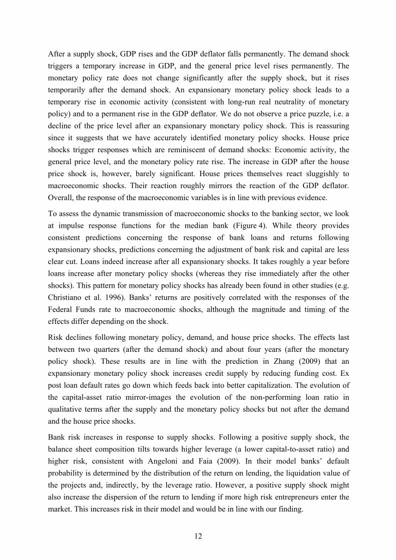
After a supply shock, GDP rises and the GDP deflator falls permanently. The demand shock triggers a temporary increase in GDP, and the general price level rises permanently. The monetary policy rate does not change significantly after the supply shock, but it rises temporarily after the demand shock. An expansionary monetary policy shock leads to a temporary rise in economic activity (consistent with long-run real neutrality of monetary policy) and to a permanent rise in the GDP deflator. We do not observe a price puzzle, i.e. a decline of the price level after an expansionary monetary policy shock. This is reassuring since it suggests that we have accurately identified monetary policy shocks. House price shocks trigger responses which are reminiscent of demand shocks: Economic activity, the general price level, and the monetary policy rate rise. The increase in GDP after the house price shock is, however, barely significant. House prices themselves react sluggishly to macroeconomic shocks. Their reaction roughly mirrors the reaction of the GDP deflator. Overall, the response of the macroeconomic variables is in line with previous evidence.

To assess the dynamic transmission of macroeconomic shocks to the banking sector, we look at impulse response functions for the median bank (Figure 4). While theory provides consistent predictions concerning the response of bank loans and returns following expansionary shocks, predictions concerning the adjustment of bank risk and capital are less clear cut. Loans indeed increase after all expansionary shocks. It takes roughly a year before loans increase after monetary policy shocks (whereas they rise immediately after the other shocks). This pattern for monetary policy shocks has already been found in other studies (e.g. Christiano et al. 1996). Banks’ returns are positively correlated with the responses of the Federal Funds rate to macroeconomic shocks, although the magnitude and timing of the effects differ depending on the shock.

Risk declines following monetary policy, demand, and house price shocks. The effects last between two quarters (after the demand shock) and about four years (after the monetary policy shock). These results are in line with the prediction in Zhang (2009) that an expansionary monetary policy shock increases credit supply by reducing funding cost. Ex post loan default rates go down which feeds back into better capitalization. The evolution of the capital-asset ratio mirror-images the evolution of the non-performing loan ratio in qualitative terms after the supply and the monetary policy shocks but not after the demand and the house price shocks.

Bank risk increases in response to supply shocks. Following a positive supply shock, the balance sheet composition tilts towards higher leverage (a lower capital-to-asset ratio) and higher risk, consistent with Angeloni and Faia (2009). In their model banks’ default probability is determined by the distribution of the return on lending, the liquidation value of the projects and, indirectly, by the leverage ratio. However, a positive supply shock might also increase the dispersion of the return to lending if more high risk entrepreneurs enter the market. This increases risk in their model and would be in line with our finding.

12

Our result of a decline in bank risk after expansionary monetary policy shocks is therefore similar to the findings by De Graeve et al. (2008) (for Germany) but not to those from other empirical studies such as Angeloni et al. (2010) or from the risk-taking channel literature.

The correlation between banks’ risk and return is negative after the demand and the house price shocks. This would be consistent with theoretical models arguing that banks with higher returns (and thus presumably higher market power) engage in less risky lending than banks with lower returns (Allen and Gale 2004, Martínez-Miera and Repullo 2008). The correlation between bank returns and risk after the supply and the monetary policy shocks depends on the horizon; it is positive at short horizons but becomes negative at medium horizons. Recent DSGE models have different implications on the correlation between risk and return. Following a monetary policy shock, this correlation is negative in Angeloni and Faia (2010) but positive in Meh and Moran (2010) or Zhang (2009).

4.1.2 Variance Decompositions

While Figure 4 provides information on the dynamic responses of (median) bank-level variables to macroeconomic shocks, Table 4 shows the forecast error variance decomposition and allows assessing the relative importance of each of these shocks. We distinguish the short run (the one-year forecast horizon) from the medium run (the five-year horizon). Macroeconomic shocks together explain 27 percent of the non-performing loans ratio, 33 percent of the capital ratio, and 12 and 14 percent of returns on assets and loans, respectively, of the median bank in the short run. These numbers increase for the ratio variables by 1-8 percentage points in the medium run and decline for loans by 2 percentage points. For risk at short horizons, house price shocks are most important, consistent with theoretical models that emphasize the role of real estate as collateral for bank loans (Goel et al. 2009). Monetary policy shocks play the biggest role for risk at medium horizons. Aggregate demand shocks account for the greatest share of the variation in loans at short horizons. At medium horizons, all shocks play an about equally discernible role for loans. An additional finding is that the idiosyncratic (variable-specific) components are about as important as common banking shocks for the non-performing loans and the capital ratios and they are more important for return on assets and loans.

Table 4 also reveals that shocks to the latent banking factors (or “banking shocks”) are quite important for macroeconomic variables. These shocks explain between 22 and 35 percent of the forecast error variance of the macroeconomic variables in the medium run. The shares are largest for house prices and for the monetary policy rate. The short-term effects are smaller, ranging between 4 percent (GDP deflator) and 26 percent (Federal Funds rate).

13

4.1.3 The Role of Bank-Level Information

We finally assess how omitting information extracted from the micro-level banking dataset would bias our results. Figure 5 compares the impulse responses of the observable macroeconomic factors derived from our benchmark FAVAR model with impulse responses obtained from a VAR in which we replace the banking factors by the median values of our bank-balance sheet variables. The responses of GDP, the GDP deflator, and house prices following macroeconomic shocks are very similar in magnitude and shape in both models. There are, however, notable differences in the responses of the Federal Funds rate after all four shocks. In particular, the VAR model without micro-level information predicts significantly larger and more persistent responses of the interest rate relative to our benchmark FAVAR model. The reason could be that monetary policy reacts to the banking factors (beyond its reaction to median bank variables).

An additional finding is that monetary policy shocks identified from the VAR model with the median banking variables are larger than the shocks extracted from the benchmark FAVAR (Figure 6). This suggests that the VAR model assigns shocks originating in the banking market to monetary policy.19 Figure 6 also reveals that our FAVAR model identifies a sequence of expansionary monetary policy shocks in 2002 and then again between 2003 and 2006. This is consistent with the general consensus of rather loose monetary policy in this period (e.g. Eickmeier and Hofmann 2010, or Taylor 2009). In contrast, the VAR ignoring the micro-level banking data would point to contractionary monetary policy shocks between 2003 and 2006. We have also compared a VAR with the four median banking variables with a VAR which includes only the four macroeconomic variables. Findings are almost identical, and we do not show results from the pure macroeconomic VAR here. Hence, information contained in the micro bank-level data seems to matter.

In sum, we find that macroeconomic shocks play a non-trivial role for developments in the banking sector. Bank risk for the median bank falls following most expansionary macroeconomic shocks, and lending increases. Furthermore, the correlation between banks’ risk and return is negative after all shocks at medium horizons. We also find that shocks to the banking factors affect the macroeconomy, especially monetary policy rates and house prices. Results should, however, be taken with caution. Our “banking factors” ( Bt ) capture shocks to banks, but they could also capture shocks to other (financial) factors. We finally show that omitting bank-level information would bias estimated impulse response functions of the monetary policy rate. It would also attribute shocks originating in the banking sector

19 We omit the identified supply, demand and house price shock series since they are very similar in both models.

14

(incorrectly) to monetary policy shocks and yield a rather implausible shape of the monetary policy shocks.

4.2 What are the Sources of Heterogeneity across Banks?

So far, we have focused on adjustments of the “median” bank following macroeconomic shocks. However, the rich structure of our dataset also allows analyzing bank heterogeneity. Bank heterogeneity has two dimensions: There may be a substantial idiosyncratic component in bank-level developments, but heterogeneity may also reflect that banks respond differently to the common shocks. Next, we analyze the importance of these sources of heterogeneity by looking at the dispersion of the common and the idiosyncratic components of bank-level developments. In a final step, we will use information on bank characteristics to explain different adjustments to macroeconomic shocks.

4.2.1 Idiosyncratic Shocks versus Asymmetric Transmission of Common Shocks

Table 5 shows the dispersion of idiosyncratic and common components of individual banks’ risk, capitalization, profitability, and lending over the sample period. Bank heterogeneity is not only due to idiosyncratic shocks but also due to the asymmetric transmission of common shocks. For all variables but the capital ratio asymmetric transmission is more important.20

To visualize the transmission of common macroeconomic shocks to individual banks we show in Figure 7 the (5th to 95th quantiles of) impulse response functions of individual banks.21 The graph reveals substantial heterogeneity after all macroeconomic shocks, in line with results by Dave et al. (2009) for the development of loans after monetary policy shocks. Although risk has been shown to decline for the median bank in response to a monetary policy loosening, Figure 7 shows that risk indeed rises for a large fraction (roughly 1/3) of banks.

4.2.2 Which Bank-Level Features Affect the Exposure of Banks to Monetary Policy and House Price Shocks?

In a next step, we analyze whether the impact of monetary policy and house price shocks differs across individual banks with different characteristics in any systematic way. We regress individual banks’ impulse response functions of risk and lending after two and four quarters on several variables which are intended to capture long-run, structural differences across banks.

We focus on monetary policy and house price shocks for three main reasons: First, house price shocks play a prominent role in theoretical studies featuring financial accelerator

20 We obtain the same qualitative result also using a larger dataset with a less stringent outlier correction. 21 We show the 5th to 95th quantiles instead of all impulse response functions for better visibility.

15

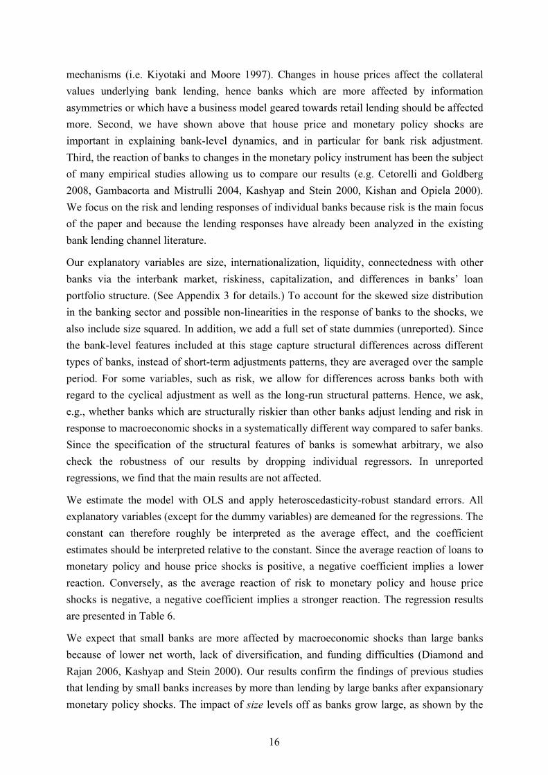
mechanisms (i.e. Kiyotaki and Moore 1997). Changes in house prices affect the collateral values underlying bank lending, hence banks which are more affected by information asymmetries or which have a business model geared towards retail lending should be affected more. Second, we have shown above that house price and monetary policy shocks are important in explaining bank-level dynamics, and in particular for bank risk adjustment. Third, the reaction of banks to changes in the monetary policy instrument has been the subject of many empirical studies allowing us to compare our results (e.g. Cetorelli and Goldberg 2008, Gambacorta and Mistrulli 2004, Kashyap and Stein 2000, Kishan and Opiela 2000). We focus on the risk and lending responses of individual banks because risk is the main focus of the paper and because the lending responses have already been analyzed in the existing bank lending channel literature.

Our explanatory variables are size, internationalization, liquidity, connectedness with other banks via the interbank market, riskiness, capitalization, and differences in banks’ loan portfolio structure. (See Appendix 3 for details.) To account for the skewed size distribution in the banking sector and possible non-linearities in the response of banks to the shocks, we also include size squared. In addition, we add a full set of state dummies (unreported). Since the bank-level features included at this stage capture structural differences across different types of banks, instead of short-term adjustments patterns, they are averaged over the sample period. For some variables, such as risk, we allow for differences across banks both with regard to the cyclical adjustment as well as the long-run structural patterns. Hence, we ask, e.g., whether banks which are structurally riskier than other banks adjust lending and risk in response to macroeconomic shocks in a systematically different way compared to safer banks. Since the specification of the structural features of banks is somewhat arbitrary, we also check the robustness of our results by dropping individual regressors. In unreported regressions, we find that the main results are not affected.

We estimate the model with OLS and apply heteroscedasticity-robust standard errors. All explanatory variables (except for the dummy variables) are demeaned for the regressions. The constant can therefore roughly be interpreted as the average effect, and the coefficient estimates should be interpreted relative to the constant. Since the average reaction of loans to monetary policy and house price shocks is positive, a negative coefficient implies a lower reaction. Conversely, as the average reaction of risk to monetary policy and house price shocks is negative, a negative coefficient implies a stronger reaction. The regression results are presented in Table 6.

We expect that small banks are more affected by macroeconomic shocks than large banks because of lower net worth, lack of diversification, and funding difficulties (Diamond and Rajan 2006, Kashyap and Stein 2000). Our results confirm the findings of previous studies that lending by small banks increases by more than lending by large banks after expansionary monetary policy shocks. The impact of size levels off as banks grow large, as shown by the

16

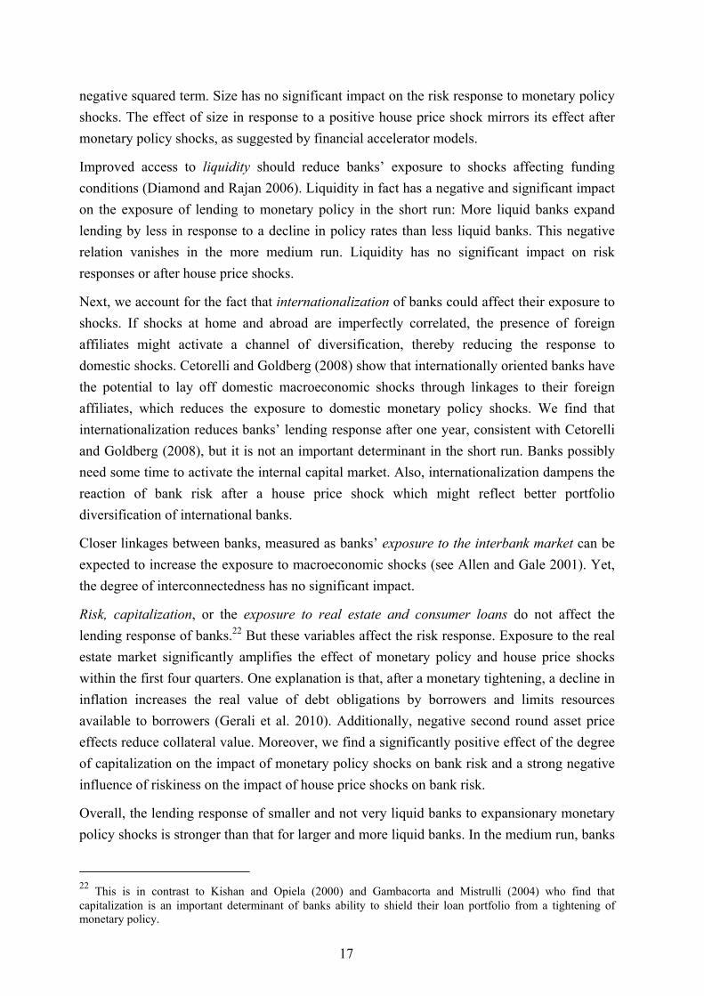
negative squared term. Size has no significant impact on the risk response to monetary policy shocks. The effect of size in response to a positive house price shock mirrors its effect after monetary policy shocks, as suggested by financial accelerator models.

Improved access to liquidity should reduce banks’ exposure to shocks affecting funding conditions (Diamond and Rajan 2006). Liquidity in fact has a negative and significant impact on the exposure of lending to monetary policy in the short run: More liquid banks expand lending by less in response to a decline in policy rates than less liquid banks. This negative relation vanishes in the more medium run. Liquidity has no significant impact on risk responses or after house price shocks.

Next, we account for the fact that internationalization of banks could affect their exposure to shocks. If shocks at home and abroad are imperfectly correlated, the presence of foreign affiliates might activate a channel of diversification, thereby reducing the response to domestic shocks. Cetorelli and Goldberg (2008) show that internationally oriented banks have the potential to lay off domestic macroeconomic shocks through linkages to their foreign affiliates, which reduces the exposure to domestic monetary policy shocks. We find that internationalization reduces banks’ lending response after one year, consistent with Cetorelli and Goldberg (2008), but it is not an important determinant in the short run. Banks possibly need some time to activate the internal capital market. Also, internationalization dampens the reaction of bank risk after a house price shock which might reflect better portfolio diversification of international banks.

Closer linkages between banks, measured as banks’ exposure to the interbank market can be expected to increase the exposure to macroeconomic shocks (see Allen and Gale 2001). Yet, the degree of interconnectedness has no significant impact.

Risk, capitalization, or the exposure to real estate and consumer loans do not affect the lending response of banks.22 But these variables affect the risk response. Exposure to the real estate market significantly amplifies the effect of monetary policy and house price shocks within the first four quarters. One explanation is that, after a monetary tightening, a decline in inflation increases the real value of debt obligations by borrowers and limits resources available to borrowers (Gerali et al. 2010). Additionally, negative second round asset price effects reduce collateral value. Moreover, we find a significantly positive effect of the degree of capitalization on the impact of monetary policy shocks on bank risk and a strong negative influence of riskiness on the impact of house price shocks on bank risk.

Overall, the lending response of smaller and not very liquid banks to expansionary monetary policy shocks is stronger than that for larger and more liquid banks. In the medium run, banks

22 This is in contrast to Kishan and Opiela (2000) and Gambacorta and Mistrulli (2004) who find that capitalization is an important determinant of banks ability to shield their loan portfolio from a tightening of monetary policy.

17

with foreign affiliates react less strongly to monetary policy shocks in terms of lending. Risk declines by more for banks highly engaged in real estate lending and for riskier banks, while better capitalized banks react less in terms of risk to monetary policy shocks. Moreover, lending of larger banks increases less in response to house prices shocks. Riskier banks react more to house price shocks while international banks react less in terms of risk.

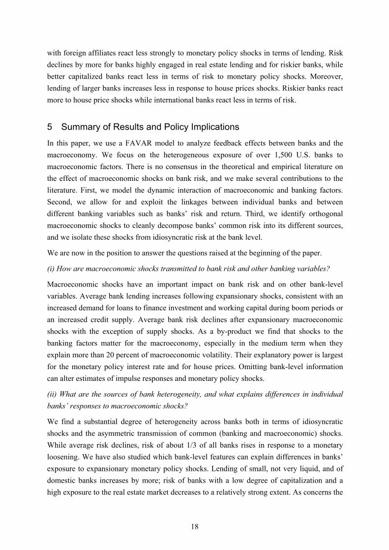
5 Summary of Results and Policy Implications

In this paper, we use a FAVAR model to analyze feedback effects between banks and the macroeconomy. We focus on the heterogeneous exposure of over 1,500 U.S. banks to macroeconomic factors. There is no consensus in the theoretical and empirical literature on the effect of macroeconomic shocks on bank risk, and we make several contributions to the literature. First, we model the dynamic interaction of macroeconomic and banking factors. Second, we allow for and exploit the linkages between individual banks and between different banking variables such as banks’ risk and return. Third, we identify orthogonal macroeconomic shocks to cleanly decompose banks’ common risk into its different sources, and we isolate these shocks from idiosyncratic risk at the bank level.

We are now in the position to answer the questions raised at the beginning of the paper.

(i) How are macroeconomic shocks transmitted to bank risk and other banking variables?

Macroeconomic shocks have an important impact on bank risk and on other bank-level variables. Average bank lending increases following expansionary shocks, consistent with an increased demand for loans to finance investment and working capital during boom periods or an increased credit supply. Average bank risk declines after expansionary macroeconomic shocks with the exception of supply shocks. As a by-product we find that shocks to the banking factors matter for the macroeconomy, especially in the medium term when they explain more than 20 percent of macroeconomic volatility. Their explanatory power is largest for the monetary policy interest rate and for house prices. Omitting bank-level information can alter estimates of impulse responses and monetary policy shocks.

(ii) What are the sources of bank heterogeneity, and what explains differences in individual banks’ responses to macroeconomic shocks?

We find a substantial degree of heterogeneity across banks both in terms of idiosyncratic shocks and the asymmetric transmission of common (banking and macroeconomic) shocks. While average risk declines, risk of about 1/3 of all banks rises in response to a monetary loosening. We have also studied which bank-level features can explain differences in banks’ exposure to expansionary monetary policy shocks. Lending of small, not very liquid, and of domestic banks increases by more; risk of banks with a low degree of capitalization and a high exposure to the real estate market decreases to a relatively strong extent. As concerns the

18

exposure to house price shocks we find that lending of larger banks increases less while risk of riskier and domestic banks reacts more after expansionary house price shocks.

Our findings are interesting from a banking regulation perspective. The result that less liquid and not well capitalized banks react more to macroeconomic shocks support proposals requiring more capital and higher liquidity ratios if regulators are concerned that the banking sector acts as an accelerator of macroeconomic shocks. At the same time, we find that small and purely domestic banks are more vulnerable to macroeconomic shocks. But one should also take into account that the systemic impact of these banks on the macroeconomy is rather small. Regulatory policy would therefore need to balance different criteria (the relevance of an institution for systemic risk and its exposure to macroeconomic shocks) when deciding upon new capital or liquidity requirements.

In terms of future research, there are three additional issues which we consider promising. First, it would be interesting to disentangle domestic and global macroeconomic shocks and to assess if internationally active banks are worse off after adverse global shocks. Second, non-linearities, e.g. in the reaction of banks to common (macroeconomic and banking) shocks, may be present in exceptional situations such as banking crises. Our model has to be seen as suitable to analyze macro-banking feedbacks in “normal” times, but could be extended to allow for non-linearities. Third, the role of shocks to large banks for macroeconomic dynamics would be worth examining in details.

Overall, our analysis can be seen as a first step into the direction of jointly modeling dynamics of the banking sector and the macroeconomy. They suggest that these feedback effects are relevant for both, understanding macroeconomic dynamics as well as the behavior of banks. Research of this type would certainly benefit from high-quality microeconomic panel data.

19

6 References

Allen, F. and D. Gale (2001). Financial Contagion. Journal of Political Economy 108(1): 1-33.

Allen, F. and D. Gale (2004). Competition and Financial Stability. Journal of Money, Credit and Banking 36(3): 453-80.

Altunbas, Y., L. Gambacorta, D. Marqués Ibañez (2009). An Empirical Assessment of the Risk-Taking Channel. University of Wales, Bank for International Settlements, and European Central Bank. Mimeo. Basel.

Angeloni, I., and E. Faia (2009). A Tale of Two Policies: Prudential Regulation and Monetary Policy with Fragile banks. Kiel Institute for die World Economy. Kiel Working Paper 1569. Kiel.

Angeloni, I., E. Faia, M. Lo Duca (2010) Monetary Policy and Risk Taking, University of Frankfurt, Mimeo.

Bai, J. and S. Ng (2002). Determining the Number of Factors in Approximate Factor Models. Econometrica 70(1): 191-221.

Bai J. and P. Perron (2003). Computation and Analysis of Multiple Structural Change Models. Journal of Applied Econometrics 18: 1-22.

Basel Committee on Banking Supervision (2009). Consultative proposals to strengthen the resilience of the banking sector announced by the Basel Committee. 17.12.2009. Basel.

Beck, G., K. Hubrich, and M. Marcellino (2009). Regional Inflation Dynamics within and across Euro Area Countries and a Comparison with the US. Economic Policy 57: 141-184.

Beck, T. (2008). Bank Competition and Financial Stability: Friends or Foes? World Bank Policy Research Working Paper 4656. Washington DC.

Berger, A. and T. Hannan (1991). The Rigidity of Prices: Evidence from the Banking Industry. American Economic Review 81(4): 938-45.

Berger, A. and C. Bouwman (2009). Bank Liquidity Creation. Review of Financial Studies 22(9): 3779-3837

Bernanke, B., M. Gertler, and S. Gilchrist (1996). The Financial Accelerator and the Flight to Quality. The Review of Economics and Statistics 78(1): 1-15.

20

Bernanke, B.S., J. Boivin, and P. Eliasz (2005). Measuring the Effects of Monetary Policy: A Factor-Augmented Vector Autoregressive (FAVAR) Approach. Quarterly Journal of Economics (February): 387-422.

Bjørnland, H., and D. H. Jacobsen (2008). The Role of House Prices in the Monetary Policy Transmission Mechanism in the US. Norges Bank Working Paper 2008/24. Oslo.

Bloom, N. (2009). The Impact of Uncertainty Shocks. Econometrica 77(3): 623-685.

Boivin, J. and S. Ng (2006). Are more data always better for factor analysis? Journal of Econometrics 132(1): 169-194.

Boivin, J. and M. P. Giannoni (2007). Global Forces and Monetary Policy Effectiveness. National Bureau of Economic Research (NBER). Chapters, in: International Dimensions of Monetary Policy: 429-478. Cambridge, MA.

Boivin, J., M. Giannoni, and I. Mihov (2009). Sticky Prices and Monetary Policy: Evidence from Disaggregated US Data. American Economic Review 99(1): 350-84.

Borio, C., and H. Zhu (2008). Capital Regulation, Risk-Taking and Monetary Policy: A Missing Link in the Transmission Mechanism?. Bank for International Settlements Working Paper, No. 268. Basel.

Boyd, J. H. and G. De Nicoló (2005), The Theory of Bank Risk Taking and Competition Revisited. The Journal of Finance 60: 1329–1343.

Brunnermeier, M.K. (2008). Deciphering the Liquidity and Credit Crunch 2007-2008. Bureau of Economic Research (NBER). Working Paper 14612. Cambridge, MA.

Canova, F., and G. De Nicoló (2003). On the Sources of Business Cycles in the G-7. Journal of International Economics, Elsevier 59(1): 77-100.

Cetorelli, N. and L. S. Goldberg (2008). Banking Globalization, Monetary Transmission, and the Lending Channel. National Bureau of Economic Research (NBER), Working Paper 14101, Cambridge MA.

Chamberlain, G., and M. Rothschild (1983). Arbitrage, Factor Structure and Mean-Variance Analysis in Large Asset Markets, Econometrica, 51, 1305-1324.

Christiano, L. J., M. Eichenbaum and C. Evans (1996). The Effects of Monetary Policy Shocks: Evidence from the Flow of Funds. The Review of Economics and Statistics 78(1): 16-34.

Ciccarelli, M., A. Maddaloni, and J.-L. Peydró (2009). Trusting the Bankers: A New Look at the Credit Channel of Monetary Policy. European Central Bank. Mimeo. Frankfurt a.M.

21

Dave, C., S.J. Dressler, and L. Zhang (2009). The Bank Lending Channel: a FAVAR Analysis. University of Texas at Dallas, Villanova University. Mimeo.

Del Negro, M., and C. Otrok (2007). 99 Luftballons: Monetary Policy and the House Price Boom Across States, Journal of Monetary Economics, 54, 1962-1985.

Den Reijer, A.H.J. (2007). Identifying Regional and Sectoral Dynamics of the Dutch Staffing Labour Cycle. DNB Working Paper 153.

De Nicoló, G., and M. Lucchetta (2010). Systemic Risk and the Macroeconomy. International Monetary Fund. IMF Working Paper 10/29. Washington DC.

De Graeve, F., T. Kick and M. Koetter (2008). Monetary policy and financial (in)stability: An integrated micro-macro approach. Journal of Financial Stability 4(3): 205-231.

Dell’Ariccia, G., and R. Marquez (2006). Lending Booms and Lending Standards. The Journal of Finance LXI(5): 2511-2546.

Diamond, D. W. and R. G. Rajan, (2006). Money in a Theory of Banking. American Economic Review 96(1): 30-53.

Dib, A (2010). Banks, Credit Market Frictions, and Business Cycles. mimeo

Eickmeier, S. (2009). Comovements and Heterogeneity in the Euro Area Analyzed in a Non-Stationary Dynamic Factor Model. Journal of Applied Econometrics 24(6): 933-959.

Eickmeier, S., B. Hofmann, and A. Worms (2009). Macroeconomic Fluctuations and Bank Lending: Evidence for Germany and the Euro Area. German Economic Review 10(2): 193-223.

Eickmeier, S., and B. Hofmann (2010). Housing Booms, Financial (Im)Balances and Monetary Policy. ECB Working Paper 1178 and Bundesbank Discussion Paper (Series 1), 07/2010. Frankfurt a.M.

Farhi, E., and J. Tirole (2009). Collective Moral Hazard, Maturity Mismatch and Systemic Bailouts. National Bureau of Economic Research (NBER). Working Paper 15138. Cambridge, MA.

Frankel, J, and G. Saravelos (2010). Are Leading Indicators of Financial Crises Useful for Assessing Country Vulnerability? Evidence from the 2008-09 Global Crisis. National Bureau of Economic Research (NBER). Working Paper 16047. Cambridge, MA.

Fry, R. and A. Pagan (2007). Some Issues in Using Sign Restrictions for Identifying Structural VARs. National Center for Economic Research (NCER). Working Paper 14. Canberra.

Gambacorta, L. and P. E Mistrulli,. (2004).Does bank capital affect lending behavior? Journal of Financial Intermediation 13(4): 436-457.

22

Gambarcorta, L. (2009). Monetary Policy and the Risk-Taking Channel. BIS Quarterly Review. December: 43-53. Basel.

Gerali, A., S. Neri, L. Sessa, F. M. Signoretti (2010). Credit and Banking in a DSGE Model of the Euro Area. Journal of Money, Credit and Banking 42: 107–141.

Gersbach, H., and V. Hahn (2009). Banking-on-The-Average Rules. CER-ETH - Center of Economic Research at ETH Zurich. Working Paper No. 09/107. Zurich.

Goel, Anand M., Fenghua Song, and Anjan V. Thakor (2009). Infectious Leverage. Federal Reserve Bank of Chicago, Pennsylvania State University, and Washington University. Mimeo.

Hellwig, M. (1997). Banks, Markets, and the Allocation of Risks in an Economy. Sonderforschungsbereich 504 Publications 97-35, Sonderforschungsbereich 504, Universität Mannheim & Sonderforschungsbereich 504, University of Mannheim.

Hellwig, M. (2009).Systemic Risk in the Financial Sector: An Analysis of the Subprime-Mortgage Financial Crisis. De Economist 157(2): 129-207.

International Monetary Fund (IMF) (2009). Global Financial Stability Report. April. Washington DC.

Ioannidou, V., Ongena, S. and Peydro, J.L., (2009).Monetary Policy, Risk-Taking, and Pricing: Evidence from a Quasi-Natural Experiment. Discussion Paper 2009-31 S, Tilburg University, Center for Economic Research.

Jarociński, M., and F. Smets (2008). House Prices and the Stance of Monetary Policy. Federal Reserve Bank of St. Louis Review 90(4): 339-65.

Jiménez, G., S. Ongena, J.L. Peydró, and J. Saurina (2007). Hazardous Times for Monetary Policy: What Do Twenty-Three Million Bank Loans Say About the Effects of Monetary Policy on Credit Risk. Bank of Spain, ECB, and Tilburg University. Mimeo.

Kashyap, A. K., and J. C. Stein (2000). What Do a Million Observations on Banks Say about the Transmission of Monetary Policy? American Economic Review 90(3): 407-428.

Kilian, L. (1998).Small-Sample Confidence Intervals For Impulse Response Functions. The Review of Economics and Statistics 80(2): 218-230.

Kishan, R. P. and T. P Opiela (2000). Bank Size, Bank Capital, and the Bank Lending Channel. Journal of Money, Credit and Banking 32(1): 121-41.

King, T. B. (2008). Discipline and Liquidity in the Interbank Market. Journal of Money, Credit and Banking 40(2-3): 295-317.

23

Kiyotaki, N. and Moore, J. (1997). Credit Cycles. Journal of Political Economy 105(2): 211-48.

Kose, A., C. Otrok, and C.H. Whiteman (2003). International Business Cycles: World, Region and Country Specific Factors. American Economic Review 93(4): 1216-1239.

Martínez-Miera, D., and R. Repullo (2010). Does Competition Reduce the Risk of Bank Failure? Review of Financial Studies 23(10): 3638-3664.

Matsuyama, K. (2007). Credit Traps and Credit Cycles. American Economic Review 97(1): 503-516.

Meh, C., and K. Moran (2010). The Role of Bank Capital in the Propagation of Shocks. Journal of Economic Dynamics and Control 34: 555-576.

Mönch, E., S. Ng, and S. Potter (2009). Dynamic Hierarchical Factor Models, Federal Reserve Bank of New York Staff Reports. 412 December. New York.

Otrok, C., and P.M. Pourpourides (2008). On the Cyclicality of Real Wages and Wage Differentials. Mimeo. University of Virginia.

Peersman, G. (2005). What Caused the Early Millennium Slowdown? Evidence based on Vector Autoregressions. Journal of Applied Econometrics 20(2): 185-207.

Rajan, R.G. (2005). Has Financial Development Made the World Riskier? National Bureau of Economic Research (NBER). Working Paper 11728. Cambridge, MA.

Rochet, J.-C. (2008). Macroeconomic Shocks and Banking Supervision. In: Rochet, Why are there so many banking crises? The Politics and Policy of Bank Regulation.

Rubio-Ramírez, J.F., D.F. Waggoner, T. Zha (2010). Structural Vector Autoregressions: Theory of Identification and Algorithms for Inference Review of Economic Studies 77(2): 665-696.

Stock, J. H. and M.W. Watson (1998). Diffusion indexes. NBER Working Paper 6702.

Stock, J. H. and M.W. Watson (2002). Macroeconomic Forecasting using Diffusion Indexes. Journal of Business and Economic Statistics 20(2): 147-162.

Stock, J. H. and M. W. Watson (2005). Implications of Dynamic Factor Models for VAR Analysis. National Bureau of Economic Research (NBER). Working Paper 11467. Cambridge, MA.

Taylor, J. (2009). The Financial Crisis and the Policy Responses: An Empirical Analysis of What Went Wrong. NBER Working Paper 14631.

Uhlig, H. (2005). What are the Effects of Monetary Policy on Output? Results from an Agnostic Identification Procedure. Journal of Monetary Economics 52: 381-419.

24

Walsh, Carl E. (2003). Monetary Theory and Policy (2nd edition). The MIT Press (Cambridge MA).

Zhang, L. (2009). Bank Capital Regulation, the Lending Channel, and Business Cycles. Deutsche Bundesbank. Discussion Paper Series 1: Economic Studies. 33/2009. Frankfurt a.M.

25

Appendix 1: Theoretical Background on the Effects of Macroeconomic Shocks on Banks

In a complete markets setting, banks should be exposed to idiosyncratic risk but they can write contracts insuring them against macroeconomic risks (Hellwig 1997). Yet, models assuming financial contracts that isolate banks from macroeconomic shocks miss important interactions between banks and the macroeconomy (Zhang 2009). Theoretical contributions explaining the exposure of banks to macroeconomic risk need to assume frictions on financial markets.

Most previous work linking banks and the macroeconomy focuses on monetary policy shocks and the lending channel. Walsh (2003) distinguishes two aspects. According to the bank lending channel, policies that affect the reserves of the banking system influence the transmission of monetary impulses. If access to uninsured funding is limited due to financial frictions, banks cut their lending in response to a tighter monetary policy, and negative output responses are reinforced. According to the financial-accelerator mechanism, the availability of cash flow and the net worth of firms affect the availability of external finance. If a recession weakens firms’ internal resources, the volume supply of credit declines, and the negative effects of the downturn are aggravated.

Recent macroeconomic models explicitly incorporate banks in DSGE models and analyze the feedback between banks and different macroeconomic shocks (Table A.1). Angeloni and Faia (2009) and Angeloni et al. (2010) analyze the impact of monetary, productivity, demand (fiscal policy), and asset price shocks. In their model, banks use equity and deposits to finance lending to entrepreneurs. Entrepreneurs have no internal funds and require financing from banks as relationship lenders. Banks have special skills in redeploying assets that are liquidated early. Since the entrepreneurs’ project outcome depends on the realization of a random shock, depositors run the bank whenever they realize that the return from the project is insufficient to serve all depositors. The model predicts that, following a positive productivity shock, inflation and interest rates fall, and output increases. In the model, the deposit rate moves one to one with the policy rate. Therefore, a decline in the interest rate corresponds to a reduction in banks’ cost of funding. A reduction in the deposit rate increases the probability that project returns are high enough to serve all claims of depositors. Consequently, banks optimally choose to increase the ratio of external funding in an attempt to maximize return to bank capital. The decline in interest rates lowers banks’ return on assets and this, together with the more fragile balance sheet composition, increases bank risk. A similar mechanism increases bank risk after an expansionary monetary policy shock.

Bank risk in the model by Angeloni and Faia (2009) is the probability of a bank run occurring, and this probability is determined by the distribution of the returns on lending, the

26

liquidation value of the projects, and indirectly on the leverage ratio. In our empirical model, the proxy for bank risk is the share of non-performing loans in total loans. This measure should be positively correlated with the definition of risk in their theoretical model.

In Angeloni and Faia (2009), the focus is on banks’ role as liquidity providers. Zhang (2009) instead focuses on an interaction between credit frictions on the demand side (net worth of firms) and the supply side (bank capital). In her model, banks and firms share macroeconomic risks because banks cannot write contracts isolating them from macroeconomic risk. Instead, loan contracts between banks and entrepreneurs are based on the expectation of future capital return and expected loan default rates. A positive technology shock, for instance, increases the return on capital above its expected value which in turn corresponds to a loan default ratio lower than expected by banks. The bank thus realizes unexpected profits on its loan portfolio. Bank capital is accumulated through these earnings, strengthening banks’ balance sheet position and consequently reducing the expected probability of default. The implications of this model differ from those in Angeloni and Faia (2009) since expansionary monetary or technology shocks lower risk.

Meh and Moran (2010) arrive at a similar conclusion in a model featuring a double moral hazard problem between banks and investors (i.e. depositors), on the one hand, and banks and firms, on the other hand. In this model bank capital mitigates the principal-agent problem between banks and depositors. By investing their own net worth into entrepreneurial projects, banks “signal” that they monitor entrepreneurs. Therefore, higher bank capital increases banks’ ability to attract loanable funds. At the same time, the amount entrepreneurs can borrow depends on their own net worth, as in a financial accelerator model. In this model, a monetary easing reduces the costs of loanable funds, leading banks to rely more on external funding to finance lending. This leads to a reduction in the capital-asset–ratio, and bank risk increases.

In the papers cited so far, changes in interest rate spreads are not modeled as a transmission mechanism of macroeconomic shocks because banks are assumed to operate under perfect competition. Gerali et al. (2010) modify this assumption by introducing monopolistic competition on the deposit and the lending side of banks’ business. Moreover, different types of transaction costs prevent banks from adjusting their interest rates and balance sheets instantaneously. Banks lend to entrepreneurs as well as to a group of “impatient” households with a high rate of time preference. While the model is very rich in terms of the structure of the banking system, it does not focus on the implications of the macroeconomy for bank risk, which is the focus of our analysis.

In sum, theoretical literature has quite clear-cut implications with regard to the impact of different macroeconomic shocks on the volume of lending and the profitability of banks. Expansionary shocks increase lending, and the returns of banks mirror changes in interest rates. Implications for the impact of these shocks on bank risk and on capitalization are less

27

clear-cut. While some papers suggest a positive correlation between expansionary shocks and bank risk, this correlation might also be negative if a financial accelerator mechanism is at work and if banks “flee to quality”.

Recent literature has also discussed the exposure of banks to macroeconomic factors as a determinant of systemic risks in banking. In Farhi and Tirole (2009), the probability of success of projects financed by banks depends on macroeconomic shocks. Banks choose the correlation of their portfolio risk with that of other banks. There is a strategic complementarity in these choices – the higher the number of banks holding similar portfolios, the more likely is a (monetary) bail out in case of a negative shock. Banks want to fail when the largest possible number of other banks is failing. One implication of the model is that a low (policy) interest rate increases risk because of increased bank leverage (a lower capital-asset-ratio). This implication would be in line with the model by Angeloni and Faia (2009).

28

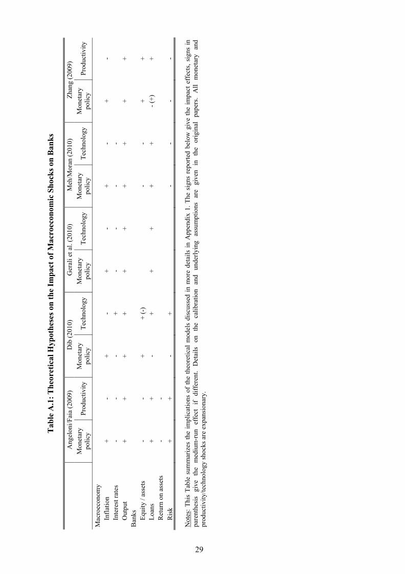
Tab

le A

.1: T

heor

etic

al H

ypot

hese

s on

the

Impa

ct o

f Mac

roec

onom

ic S

hock

s on

Ban

ks

A

ngel

oni/F

aia

(200

9)

Dib

(201

0)

Ger

ali e

t al.

(201

0)

Meh

/Mor

an (2

010)

Zh

ang

(200

9)

M

onet

ary

polic

y Pr

oduc

tivity

M

onet

ary

polic

y Te

chno

logy

M

onet

ary

polic

y Te

chno

logy

M

onet

ary

polic

y Te

chno

logy

M

onet

ary

polic

y Pr

oduc

tivity

Mac

roec

onom

y

In

flatio

n +

- +

- +

- +

- +

- In

tere

st ra

tes

- -

- +

- -

- -

Out

put

+ +

+ +

+ +

+ +

+ +

Ban

ks

Equi

ty /

asse

ts

- -

+ +

(-)

- -

+ +

Loan

s +

+ -

+ +

+ +

+ - (

+)

+ R

etur

n on

ass

ets

- -

Ris

k

+ +

- +

- -

- -

Not

es: T

his

Tabl

e su

mm

ariz

es th

e im

plic

atio

ns o

f th

e th

eore

tical

mod

els

disc

usse

d in

mor

e de

tails

in A

ppen

dix

1. T

he s

igns

rep

orte

d be

low

giv

e th

e im

pact

eff

ects

, sig

ns in

pa

rent

hesi

s gi

ve

the

med

ium

-run

ef

fect

if

diff

eren

t. D

etai

ls

on

the

calib

ratio

n an

d un

derly

ing

assu

mpt

ions

ar

e gi

ven

in

the

orig

inal

pa

pers

. A

ll m

onet

ary

and

prod

uctiv

ity/te

chno

logy

shoc

ks a

re e

xpan

sion

ary.

29

Appendix 2: Identification of Shocks

Suppose that tu is the 1r M+ × vector of reduced-form VAR residuals where the latent and observable factors are the endogenous variables. The 1r M+ × vector of (orthogonalized) Cholesky residuals tv is estimated as

ˆˆ ˆv Aut t= , (A1)

where A is the lower triangular Cholesky matrix of )ucov( t . We partition vt in two parts, the 2 1× vector of Cholesky residuals associated with GDP growth and GDP deflator inflation 1...2vt and the 2 1 1r M+ − + × vector of Cholesky residuals associated with house price inflation, the Federal Funds rate and the latent banking factors 3...v r M

t+ , and

1...2 3...ˆ ˆ ˆv = v ' v ' 'r Mt t t

+⎡ ⎤⎣ ⎦ . The estimated vector of structural shocks 1...2 3...ˆ ˆ ˆw w ' w ' 'r Mt t t

+⎡ ⎤= ⎣ ⎦ is related to vt as follows. Let 1...2 1...2ˆ ˆw =vt t and 3... 3...ˆ ˆw =Rvr M r M

t t+ + where R is the 2 2× rotation

matrix and 2R'R I= and, by construction, ˆcov(w ) It r M+= .

The rotation matrix R is chosen such that the identifying restrictions specified in the main text are satisfied. We follow Rubio-Ramírez et al. (2010) and let Ω be an 2 2× random matrix with each element having an independent standard normal distribution and QRΩ = be the QR decomposition of Ω .

It turns out that more than one R satisfy the sign restrictions. Following Fry and Pagan (2007) we choose out of K R s that satisfy the sign restrictions, the R that leads to impulse response functions which are as close as possible to their median values; for details see Fry and Pagan (2007). K is set at 100 to keep it computationally tractable.

30

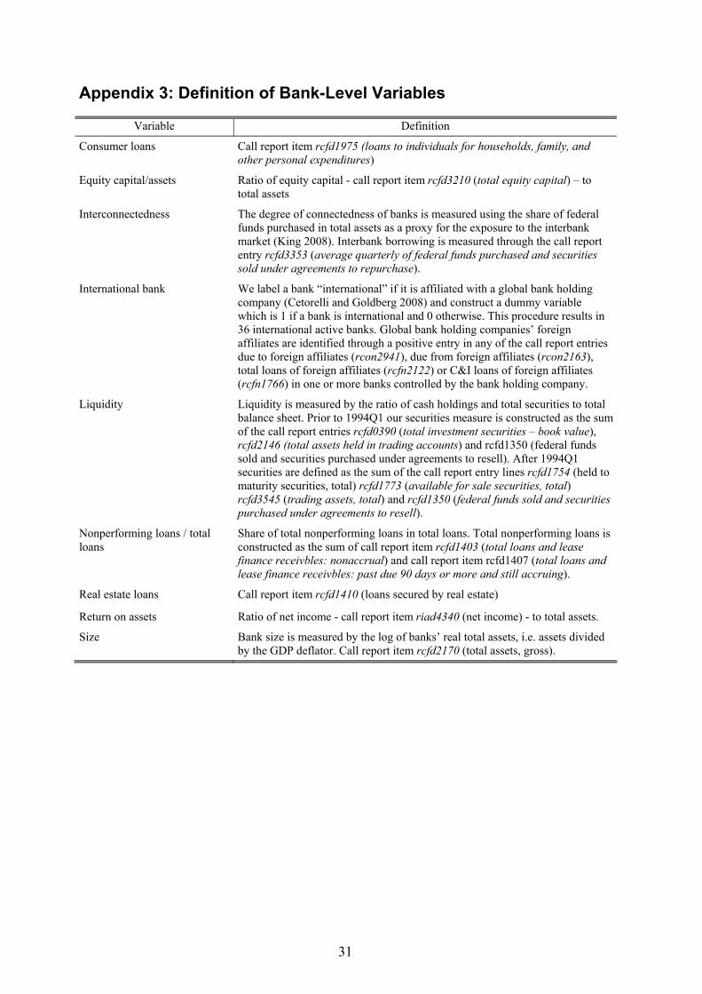
Appendix 3: Definition of Bank-Level Variables

Variable Definition

Consumer loans Call report item rcfd1975 (loans to individuals for households, family, and other personal expenditures)

Equity capital/assets Ratio of equity capital - call report item rcfd3210 (total equity capital) – to total assets

Interconnectedness The degree of connectedness of banks is measured using the share of federal funds purchased in total assets as a proxy for the exposure to the interbank market (King 2008). Interbank borrowing is measured through the call report entry rcfd3353 (average quarterly of federal funds purchased and securities sold under agreements to repurchase).

International bank We label a bank “international” if it is affiliated with a global bank holding company (Cetorelli and Goldberg 2008) and construct a dummy variable which is 1 if a bank is international and 0 otherwise. This procedure results in 36 international active banks. Global bank holding companies’ foreign affiliates are identified through a positive entry in any of the call report entries due to foreign affiliates (rcon2941), due from foreign affiliates (rcon2163), total loans of foreign affiliates (rcfn2122) or C&I loans of foreign affiliates (rcfn1766) in one or more banks controlled by the bank holding company.

Liquidity Liquidity is measured by the ratio of cash holdings and total securities to total balance sheet. Prior to 1994Q1 our securities measure is constructed as the sum of the call report entries rcfd0390 (total investment securities – book value), rcfd2146 (total assets held in trading accounts) and rcfd1350 (federal funds sold and securities purchased under agreements to resell). After 1994Q1 securities are defined as the sum of the call report entry lines rcfd1754 (held to maturity securities, total) rcfd1773 (available for sale securities, total) rcfd3545 (trading assets, total) and rcfd1350 (federal funds sold and securities purchased under agreements to resell).

Nonperforming loans / total loans

Share of total nonperforming loans in total loans. Total nonperforming loans is constructed as the sum of call report item rcfd1403 (total loans and lease finance receivbles: nonaccrual) and call report item rcfd1407 (total loans and lease finance receivbles: past due 90 days or more and still accruing).

Real estate loans Call report item rcfd1410 (loans secured by real estate)

Return on assets Ratio of net income - call report item riad4340 (net income) - to total assets.

Size Bank size is measured by the log of banks’ real total assets, i.e. assets divided by the GDP deflator. Call report item rcfd2170 (total assets, gross).

31

Table 1: Correlation Between Median Banking Variables

Non-performing loans / total loans

Equity capital / assets Return on assets Change in loans

Non-performing loans / loans 1.00 Equity capital / assets -0.89 1.00 Return on assets -0.34 0.41 1.00 Change in loans -0.30 0.28 0.40 1.00

Notes: This table shows the correlation matrix of the median banks’ variables over the entire sample period 1985Q1 – 2008Q2.

Table 2: Cumulated Variance Shares Explained by the First 15 Principal Components Calculated from Datasets Associated with Individual Banking Variables

Non-performing loans / total loans Equity capital / assets Return on assets Change in loans

1 0.14 0.16 0.12 0.10 2 0.21 0.27 0.20 0.17 3 0.28 0.35 0.27 0.23 4 0.33 0.42 0.33 0.29 5 0.38 0.48 0.38 0.33 6 0.43 0.52 0.42 0.37 7 0.46 0.56 0.45 0.40 8 0.50 0.60 0.49 0.43 9 0.52 0.63 0.51 0.45

10 0.55 0.65 0.53 0.47 11 0.57 0.67 0.55 0.49 12 0.60 0.69 0.57 0.51 13 0.62 0.70 0.59 0.53 14 0.63 0.72 0.61 0.54 15 0.65 0.73 0.62 0.56

Notes: This table shows the variance shares explained by 1 up to 15 principal components. The principal components are extracted from data sets corresponding to one bank level variable´.

32

Table 3: Identifying Restrictions

Supply Demand House price Monetary policy Shocks to latent shocks shocks shocks shocks (banking) factorsGDP + + 0 0 0 GDP deflator - + 0 0 0 House price 0 0 Federal Funds rate + Banking factors 0

Notes: The sign restrictions are imposed contemporaneously and on the first four lags after the shocks. The zero restrictions are imposed contemporaneously.

Table 4: Forecast Error Variance Decomposition

Supply shocks

Demand shocks

House price shocks

Monetary policy shocks

Shocks to latent

(banking) factors

Idiosyncratic shocks

1-year horizon GDP 0.57 0.28 0.01 0.00 0.09 GDP deflator 0.45 0.40 0.05 0.02 0.04 House price 0.03 0.02 0.83 0.00 0.08 Federal Funds rate 0.02 0.40 0.12 0.13 0.26 Non-performing loans / loans 0.05 0.06 0.10 0.06 0.30 0.39 Equity capital / assets 0.07 0.18 0.04 0.04 0.28 0.36 Return on assets 0.08 0.03 0.01 0.00 0.10 0.77 Loans 0.05 0.06 0.03 0.00 0.09 0.74 5-year horizon GDP 0.46 0.11 0.04 0.02 0.26 GDP deflator 0.36 0.22 0.03 0.05 0.22 House price 0.03 0.03 0.48 0.01 0.31 Federal Funds rate 0.03 0.32 0.12 0.12 0.35 Non-performing loans / loans 0.04 0.10 0.08 0.13 0.34 0.23 Equity capital / assets 0.05 0.16 0.03 0.10 0.36 0.21 Return on assets 0.07 0.04 0.02 0.00 0.21 0.64 Loans 0.03 0.03 0.03 0.03 0.32 0.48

Notes: The forecast error variance of the banking variables refers to the median bank.

Table 5: Dispersion of Common and Idiosyncratic Components

Non-performing loans / total loans

Equity capital / assets Return on assets Change in loans

Common component 0.70 0.53 0.81 0.84 Idiosyncratic component 0.63 0.77 0.50 0.49

Notes: This table shows the cross-sectional standard deviations on average over the sample period.

33

Tab

le 6

: Reg

ress

ion

Res

ults

M

onet

ary

polic

y sh

ock

Hou

se p

rice

shoc

k

Loan

s, ½

yea

r Lo

ans,

1 ye

ar

Ris

k, ½

yea

r R

isk,

1ye

ar

Loan

s, ½

yea

r Lo

ans,

1 ye

ar

Ris

k, ½

yea

r R

isk,

1ye

ar

Size

-0

.695

***

-1.2

43**

* -0

.019

-0

.008

-1

.476

***

-2.2

65**

* 0.

053

0.09

2

(0.2

09)

(0.4

10)

(0.0

36)

(0.0

24)

(0.4

20)

(0.6

84)

(0.0

86)

(0.0

64)

Squa

red

size

0.

030*

**

0.05

4***

0.

001

0.00

0 0.

063*

**

0.09

7***

-0

.003

-0

.004

(0.0

09)

(0.0

17)

(0.0

02)

(0.0

01)

(0.0

18)

(0.0

29)

(0.0

04)

(0.0

03)

Con

nect

edne

ss

0.19

1 0.

621

0.01

6 -0

.022

-0

.699

-1

.287

0.

004

-0.0

09

(0

.452

) (0

.892

) (0

.067

) (0

.048

) (0

.905

) (1

.351

) (0

.104

) (0

.047

) Li

quid

ity

-0.1

77*

-0.2

22

0.00

7 -0

.005

0.

036

0.39

5 0.

01

-0.0

1

(0.0

97)

(0.1

87)

(0.0

18)

(0.0

13)

(0.1

97)

(0.2

88)

(0.0

25)

(0.0

12)

Cap

italiz

atio

n 0.

163

0.34

2 0.

043

0.08

7**

-0.5

79

-0.6

87

0.09

0.

016

(0

.300

) (0

.566

) (0

.054

) (0

.037

) (0

.642

) (0

.928

) (0

.087

) (0

.040

) R

isk

-0.1

81

-0.8

32

0.13

3 -0

.159

-1

.31

-0.8

14

-0.8

86**

-0

.574

***

(0

.964

) (1

.857

) (0

.219

) (0

.158

) (2

.049

) (2

.879

) (0

.360

) (0

.159

) C

onsu

mer

loan

s / to

tal l

oans

-0

.015

-0

.079

-0

.016

0.

003

-0.1

08

-0.1

06

0.04

0.

017

(0

.108

) (0

.207

) (0

.016

) (0

.011

) (0

.202

) (0

.290

) (0

.026

) (0

.012

) R

eal e

stat

e lo

ans /

tota

l loa

ns

0.09

6 0.

121

-0.0

33**

* -0

.015

* 0.

185

0.23

1 -0

.041

**

0.02

0**

(0

.065

) (0

.126

) (0

.012

) (0

.009

) (0

.138

) (0

.194

) (0

.019

) (0

.008

) In

tern

atio

nal d

umm

y -0

.066

-0

.181

* -0

.011

0.

000

-0.0

39

-0.0

35

0.02

7**

0.00

4

(0.0

53)

(0.1

09)

(0.0

11)

(0.0

07)

(0.0

93)

(0.1

38)

(0.0

11)

(0.0

05)

Con

stan

t 0.

054

0.13

8*

-0.0

07

-0.0

15**

* 0.

098

0.20

5*

-0.0

37**

* -0

.011

*

(0.0

42)

(0.0

81)

(0.0

08)

(0.0

05)

(0.0

91)

(0.1

22)

(0.0

14)

(0.0

06)

Num

ber o

f ban

ks

1512

15

12

1512

15

12

1512

15

12

1512

15

12

R²

0.07

3 0.

072

0.06

1 0.

082

0.06

1 0.

055

0.11

3 0.

077

Not

es: T

he d

epen

dent

var

iabl

e is

the

impu

lse

resp

onse

func

tions

for t

he n

on-p

erfo

rmin

g lo

ans r

atio

and

loan

s to

expa

nsio

nary

mon

etar

y po

licy

and

hous

e pr

ice

shoc

ks.

Expl

anat

ory

varia

bles

are

dem

eane

d ba

nk c

hara

cter

istic

s as d

efin

ed in

Sec

tion

3.2.

For

mor

e de

tails

, see

als

o ta

ble

App

endi

x 3.

A fu

ll se

t of s

tate

dum

mie

s is i

nclu

ded.

***

, **,

*

= si

gnifi

canc

e at

the

1%, 5

%, 1

0%-le

vel.

Het

eros

ceda

stic

ity-r

obus

t sta

ndar

d er

rors

are

in b

rack

ets.

34

Figure 1: Kernel Densities of Banking Variables – Balanced versus Unbalanced Data

0 10 20 30 40 500

0.2

0.4Non-performing loans/loans

5 10 15 20 250

0.05

0.1

0.15

0.2

0.25Equity capital/assets

-2 -1 0 1 2 3 40

0.2

0.4

0.6

0.8

1Return on assets

9 10 11 12 13 14 15 160

0.2

0.6

0.6log Loans

Notes: Dashed red and solid black lines show kernel density estimates of unbalanced and balanced dataset respectively. The support used to estimate the kernel densities is given by the 1st and 99th percentile of the distribution of the unbalanced dataset.

35

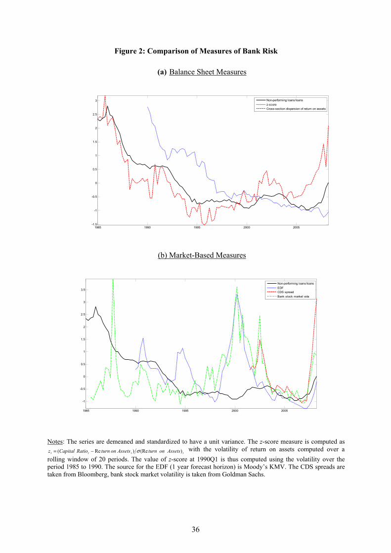
Figure 2: Comparison of Measures of Bank Risk

(a) Balance Sheet Measures

1985 1990 1995 2000 2005-1.5

-1

-0.5

0

0.5

1

1.5

2

2.5

3

Non-performing loans/loansz-scoreCross-section dispersion of return on assets

(b) Market-Based Measures

1985 1990 1995 2000 2005

-1

-0.5

0

0.5

1

1.5

2

2.5

3

3.5

Non-performing loans/loansEDFCDS spreadBank stock market vola

Notes: The series are demeaned and standardized to have a unit variance. The z-score measure is computed as tttt AssetsonturnAssetsonturnRatioCapitalz )(Re)Re( σ−= with the volatility of return on assets computed over a

rolling window of 20 periods. The value of z-score at 1990Q1 is thus computed using the volatility over the period 1985 to 1990. The source for the EDF (1 year forecast horizon) is Moody’s KMV. The CDS spreads are taken from Bloomberg, bank stock market volatility is taken from Goldman Sachs.

36

Figu

re 3

: Im

puls

e R

espo

nse

Func

tions

of M

acro

econ

omic

Fac

tors

05

1015

200

0.1

0.2

0.3

GD

PSupply

05

1015

20

-0.1

-0.0

50G

DP

def

lato

r

05

1015

20

-0.3

-0.2

-0.10

0.1

Hou

se p

rice

05

1015

20

-0.0

50

0.050.1

FFR

05

1015

200

0.1

0.2

Demand

05

1015

200

0.050.1

05

1015

20

-0.20

0.2

05

1015

20

0

0.1

0.2

0.3

05

1015

20-0

.15

-0.1

-0.0

500.

05

House price

05

1015

20

0

0.02

0.04

05

1015

200

0.2

0.4

0.6

0.8

05

1015

20

0

0.1

0.2

05

1015

20

0

0.050.1

Monetary policy

05

1015

200

0.02

0.04

05

1015

20-0

.10

0.1

0.2

05

1015

20-0

.2

-0.10

Not

es: W

e sh

ow th

e m

edia

n an

d th

e on

e st

anda

rd d

evia

tion

conf

iden

ce b

ands

. In

perc

ent (

GD

P, th

e G

DP

defla

tor a

nd h

ouse

pric

es) a

nd in

per

cent

age

poin

ts (F

eder

al F

unds

rate

).

37

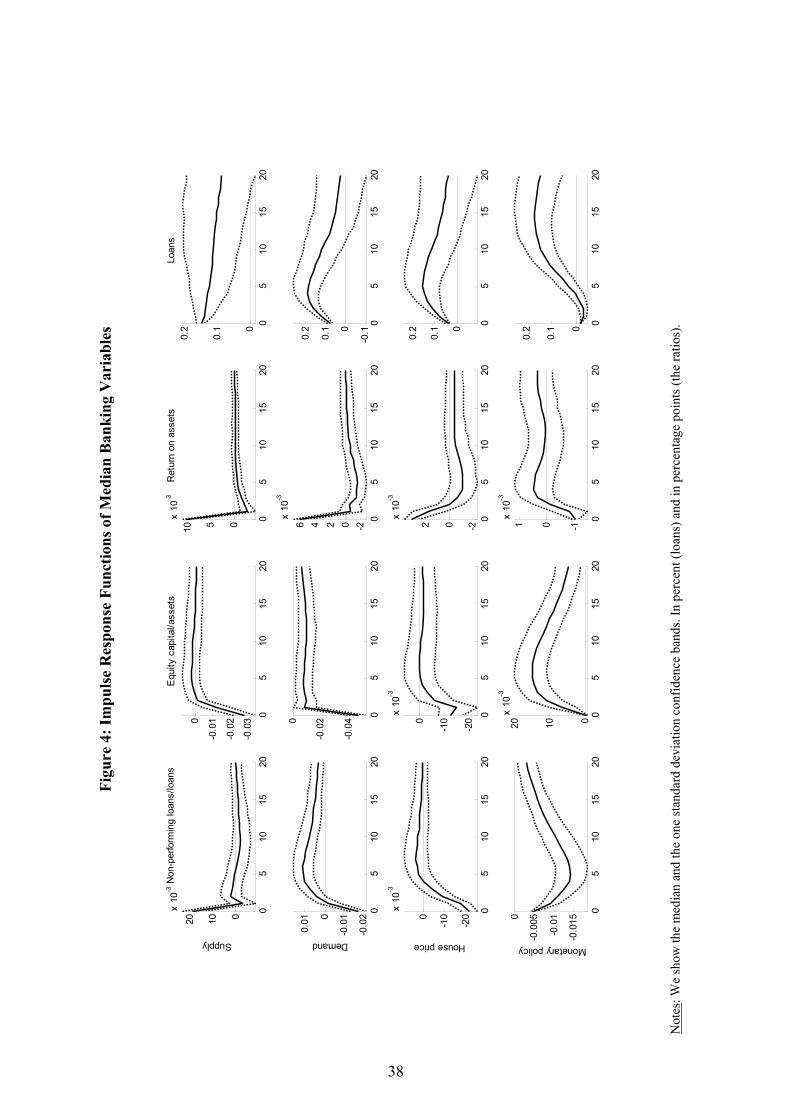
Figu

re 4

: Im

puls

e R

espo

nse

Func

tions

of M

edia

n B

anki

ng V

aria

bles

05

1015

20

01020x

10-3

Non

-per

form

ing

loan

s/lo

ans

Supply

05

1015

20-0

.03

-0.0

2

-0.0

10

Equ

ity c

apita

l/ass

ets

05

1015

20

0510x

10-3

Ret

urn

on a

sset

s

05

1015

200

0.1

0.2

Loan

s

05

1015

20-0

.02

-0.0

10

0.01

Demand

05

1015

20

-0.0

4

-0.0

20

05

1015

20-20246

x 10

-3

05

1015

20-0

.10

0.1

0.2

05

1015

20

-20

-100

x 10

-3

House price

05

1015

20

-20

-100

x 10

-3

05

1015

20-202

x 10

-3

05

1015

20

0

0.1

0.2

05

1015

20

-0.0

15

-0.0

1

-0.0

050

Monetary policy

05

1015

2001020

x 10

-3

05

1015

20

-101x

10-3

05

1015

20

0

0.1

0.2

Not

es: W

e sh

ow th

e m

edia

n an

d th

e on

e st

anda

rd d

evia

tion

conf

iden

ce b

ands

. In

perc

ent (

loan

s) a

nd in

per

cent

age

poin

ts (t

he ra

tios)

.

38

Figu

re 5

: Im

puls

e R

espo

nse

Func

tions

of M

acro

econ

omic

Fac

tors

from

the

Bas

elin

e FA

VA

R a

nd a

VA

R W

ithou

t Mic

ro-L

evel

In

form

atio

n

05

1015

024x

10-3

supplyG

DP

05

1015

-1.5-1

-0.50

x 10

-3G

DP d

efla

tor

05

1015

-4-20

x 10

-3Ho

use

pric

e

05

1015

0

0.1

0.2

FFR

05

1015

0123

x 10

-3

demand

05

1015

0

0.51

x 10

-3

05

1015

-8-6-4-202x

10-3

05

1015

0

0.1

0.2

0.3

05

1015

-101

x 10

-3

House Price

05

1015

-505

x 10

-4

05

1015

0

0.00

5

0.01

0.01

5

05

1015

0

0.1

0.2

0.3

05

1015

0510

x 10

-4

Monetary Policy

05

1015

024

x 10

-4

05

1015

024x

10-3

05

1015

-0.2

-0.10

Not

es: W

e sh

ow th

e m

edia

n an

d th

e on

e st

anda

rd d

evia

tion

conf

iden

ce b

ands

of

the

benc

hmar

k FA

VA

R m

odel

(bl

ack)

and

a s

tand

ard

VA

R w

ith th

e fo

ur m

edia

n ba

nkin

g va

riabl

es (r

ed).

In p

erce

nt (l

oans

) and

in p

erce

ntag

e po

ints

(the

ratio

s). T

he s

ize

of th

e sh

ocks

(i.e

. the

con

tem

pora

neou

s im

pact

of s

uppl

y an

d de

man

d sh

ocks

on

GD

P, o

f hou

se

pric

e sh

ocks

on

hous

e pr

ices

and

of m

onet

ary

polic

y sh

ocks

on

the

Fede

ral F

unds

rate

) obt

aine

d fr

om th

e V

AR

was

stan

dard

ized

to b

e th

e sa

me

as th

e si

ze o

f the

shoc

ks o

btai

ned

from

the

FAV

AR

.

39

Figu

re 6

: Mon

etar

y Po

licy

Shoc

k Se

ries

1990

1995

2000

2005

-4-3-2-10123

Not

es: S

hock

s est

imat

ed b

ased

on

the

benc

hmar

k FA

VA

R, i

.e. t

he m

odel

incl

udin

g ba

nk-le

vel i

nfor

mat

ion,

(sol

id b

lack

) and

the

VA

R w

ith th

e m

edia

n ba

nkin

g va

riabl

es (d

ashe

d re

d). T

he si

ze o

f the

shoc

ks is

one

stan

dard

dev

iatio

n.

40

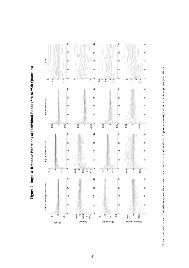
Figu

re 7

: Im

puls

e R

espo

nse

Func

tions

of I

ndiv

idua

l Ban

ks (5

th to

95t

h Q

uant

iles)

05

1015

20

-0.10

0.1

Non

-per

form

ing

loan

s/lo

ans

Supply

05

1015

20

-0.10

0.1

Equ

ity c

apita

l/ass

ets

05

1015

20-0

.050

0.05

Ret

urn

on a

sset

s

05

1015

20

-0.50

0.51

Loan

s

05

1015

20

-0.1

5-0

.1-0

.050

0.05

Demand

05

1015

20-0

.15

-0.1

-0.0

50

0.05

05

1015

20-0

.050

0.05

05

1015

20-101

05

1015

20-0

.2

-0.10

0.1

House price

05

1015

20

-0.10

0.1

05

1015

20-0

.050

0.05

05

1015

20

-0.50

0.51

1.5

05

1015

20

-0.0

50

0.05

Monetary policy

05

1015

20

-0.0

50

0.05

05

1015

20

-0.0

20

0.02

05

1015

20

-0.50

0.51

Not

es: P

oint

est

imat

es o

f im

puls

e re

spon

se fu

nctio

ns to

one

stan

dard

dev

iatio

n sh

ock.

In p

erce

nt (l

oans

) and

in p

erce

ntag

e po

ints

(the

ratio

s).

41

42

The following Discussion Papers have been published since 2009:

Series 1: Economic Studies

01 2009 Spillover effects of minimum wages Christoph Moser in a two-sector search model Nikolai Stähler 02 2009 Who is afraid of political risk? Multinational Iris Kesternich firms and their choice of capital structure Monika Schnitzer 03 2009 Pooling versus model selection for Vladimir Kuzin nowcasting with many predictors: Massimiliano Marcellino an application to German GDP Christian Schumacher 04 2009 Fiscal sustainability and Balassone, Cunha, Langenus policy implications for the euro area Manzke, Pavot, Prammer Tommasino 05 2009 Testing for structural breaks Jörg Breitung in dynamic factor models Sandra Eickmeier 06 2009 Price convergence in the EMU? Evidence from micro data Christoph Fischer 07 2009 MIDAS versus mixed-frequency VAR: V. Kuzin, M. Marcellino nowcasting GDP in the euro area C. Schumacher 08 2009 Time-dependent pricing and New Keynesian Phillips curve Fang Yao 09 2009 Knowledge sourcing: Tobias Schmidt legitimacy deficits for MNC subsidiaries? Wolfgang Sofka 10 2009 Factor forecasting using international targeted predictors: the case of German GDP Christian Schumacher

43

11 2009 Forecasting national activity using lots of international predictors: an application to Sandra Eickmeier New Zealand Tim Ng 12 2009 Opting out of the great inflation: Andreas Beyer, Vitor Gaspar German monetary policy after the Christina Gerberding breakdown of Bretton Woods Otmar Issing 13 2009 Financial intermediation and the role Stefan Reitz of price discrimination in a two-tier market Markus A. Schmidt, Mark P. Taylor 14 2009 Changes in import pricing behaviour: the case of Germany Kerstin Stahn 15 2009 Firm-specific productivity risk over the Ruediger Bachmann business cycle: facts and aggregate implications Christian Bayer 16 2009 The effects of knowledge management Uwe Cantner on innovative success – an empirical Kristin Joel analysis of German firms Tobias Schmidt 17 2009 The cross-section of firms over the business Ruediger Bachmann cycle: new facts and a DSGE exploration Christian Bayer 18 2009 Money and monetary policy transmission in the euro area: evidence from FAVAR- and VAR approaches Barno Blaes 19 2009 Does lowering dividend tax rates increase dividends repatriated? Evidence of intra-firm Christian Bellak cross-border dividend repatriation policies Markus Leibrecht by German multinational enterprises Michael Wild 20 2009 Export-supporting FDI Sebastian Krautheim

44

21 2009 Transmission of nominal exchange rate changes to export prices and trade flows Mathias Hoffmann and implications for exchange rate policy Oliver Holtemöller 22 2009 Do we really know that flexible exchange rates facilitate current account adjustment? Some new empirical evidence for CEE countries Sabine Herrmann 23 2009 More or less aggressive? Robust monetary Rafael Gerke policy in a New Keynesian model with Felix Hammermann financial distress Vivien Lewis 24 2009 The debt brake: business cycle and welfare con- Eric Mayer sequences of Germany’s new fiscal policy rule Nikolai Stähler 25 2009 Price discovery on traded inflation expectations: Alexander Schulz Does the financial crisis matter? Jelena Stapf 26 2009 Supply-side effects of strong energy price Thomas A. Knetsch hikes in German industry and transportation Alexander Molzahn 27 2009 Coin migration within the euro area Franz Seitz, Dietrich Stoyan Karl-Heinz Tödter 28 2009 Efficient estimation of forecast uncertainty based on recent forecast errors Malte Knüppel 29 2009 Financial constraints and the margins of FDI C. M. Buch, I. Kesternich A. Lipponer, M. Schnitzer 30 2009 Unemployment insurance and the business cycle: Stéphane Moyen Prolong benefit entitlements in bad times? Nikolai Stähler 31 2009 A solution to the problem of too many instruments in dynamic panel data GMM Jens Mehrhoff

45

32 2009 Are oil price forecasters finally right? Stefan Reitz Regressive expectations toward more Jan C. Rülke fundamental values of the oil price Georg Stadtmann 33 2009 Bank capital regulation, the lending channel and business cycles Longmei Zhang 34 2009 Deciding to peg the exchange rate in developing countries: the role of Philipp Harms private-sector debt Mathias Hoffmann 35 2009 Analyse der Übertragung US-amerikanischer Schocks auf Deutschland auf Basis eines FAVAR Sandra Eickmeier 36 2009 Choosing and using payment instruments: Ulf von Kalckreuth evidence from German microdata Tobias Schmidt, Helmut Stix 01 2010 Optimal monetary policy in a small open economy with financial frictions Rossana Merola 02 2010 Price, wage and employment response Bertola, Dabusinskas to shocks: evidence from the WDN survey Hoeberichts, Izquierdo, Kwapil Montornès, Radowski 03 2010 Exports versus FDI revisited: C. M. Buch, I. Kesternich Does finance matter? A. Lipponer, M. Schnitzer 04 2010 Heterogeneity in money holdings Ralph Setzer across euro area countries: Paul van den Noord the role of housing Guntram Wolff 05 2010 Loan supply in Germany U. Busch during the financial crises M. Scharnagl, J. Scheithauer

46

06 2010 Empirical simultaneous confidence Òscar Jordà, Malte Knüppel regions for path-forecasts Massimiliano Marcellino 07 2010 Monetary policy, housing booms Sandra Eickmeier and financial (im)balances Boris Hofmann 08 2010 On the nonlinear influence of Stefan Reitz Reserve Bank of Australia Jan C. Ruelke interventions on exchange rates Mark P. Taylor 09 2010 Banking and sovereign risk S. Gerlach in the euro area A. Schulz, G. B. Wolff 10 2010 Trend and cycle features in German residential investment before and after reunification Thomas A. Knetsch 11 2010 What can EMU countries’ sovereign bond spreads tell us about market perceptions of default probabilities Niko Dötz during the recent financial crisis? Christoph Fischer 12 2010 User costs of housing when households face Tobias Dümmler a credit constraint – evidence for Germany Stephan Kienle 13 2010 Extraordinary measures in extraordinary times – public measures in support of the financial Stéphanie Marie Stolz sector in the EU and the United States Michael Wedow 14 2010 The discontinuous integration of Western Europe’s heterogeneous market for corporate control from 1995 to 2007 Rainer Frey 15 2010 Bubbles and incentives: Ulf von Kalckreuth a post-mortem of the Neuer Markt in Germany Leonid Silbermann

47

16 2010 Rapid demographic change and the allocation of public education resources: evidence from East Germany Gerhard Kempkes 17 2010 The determinants of cross-border bank flows to emerging markets – new empirical evidence Sabine Herrmann on the spread of financial crisis Dubravko Mihaljek 18 2010 Government expenditures and unemployment: Eric Mayer, Stéphane Moyen a DSGE perspective Nikolai Stähler 19 2010 NAIRU estimates for Germany: new evidence on the inflation-unemployment trade-off Florian Kajuth 20 2010 Macroeconomic factors and Claudia M. Buch micro-level bank risk Sandra Eickmeier, Esteban Prieto

48

Series 2: Banking and Financial Studies 01 2009 Dominating estimators for the global Gabriel Frahm minimum variance portfolio Christoph Memmel 02 2009 Stress testing German banks in a Klaus Düllmann downturn in the automobile industry Martin Erdelmeier 03 2009 The effects of privatization and consolidation E. Fiorentino on bank productivity: comparative evidence A. De Vincenzo, F. Heid from Italy and Germany A. Karmann, M. Koetter 04 2009 Shocks at large banks and banking sector Sven Blank, Claudia M. Buch distress: the Banking Granular Residual Katja Neugebauer 05 2009 Why do savings banks transform sight deposits into illiquid assets less intensively Dorothee Holl than the regulation allows? Andrea Schertler 06 2009 Does banks’ size distort market prices? Manja Völz Evidence for too-big-to-fail in the CDS market Michael Wedow 07 2009 Time dynamic and hierarchical dependence Sandra Gaisser modelling of an aggregated portfolio of Christoph Memmel trading books – a multivariate nonparametric Rafael Schmidt approach Carsten Wehn 08 2009 Financial markets’ appetite for risk – and the challenge of assessing its evolution by risk appetite indicators Birgit Uhlenbrock 09 2009 Income diversification in the Ramona Busch German banking industry Thomas Kick 10 2009 The dark and the bright side of liquidity risks: evidence from open-end real estate funds in Falko Fecht Germany Michael Wedow

49

11 2009 Determinants for using visible reserves Bornemann, Homölle in German banks – an empirical study Hubensack, Kick, Pfingsten 12 2009 Margins of international banking: Claudia M. Buch Is there a productivity pecking order Cathérine Tahmee Koch in banking, too? Michael Koetter 13 2009 Systematic risk of CDOs and Alfred Hamerle, Thilo Liebig CDO arbitrage Hans-Jochen Schropp 14 2009 The dependency of the banks’ assets and Christoph Memmel liabilities: evidence from Germany Andrea Schertler 15 2009 What macroeconomic shocks affect the German banking system? Analysis in an Sven Blank integrated micro-macro model Jonas Dovern 01 2010 Deriving the term structure of banking Stefan Eichler crisis risk with a compound option Alexander Karmann approach: the case of Kazakhstan Dominik Maltritz 02 2010 Recovery determinants of distressed banks: Thomas Kick Regulators, market discipline, Michael Koetter or the environment? Tigran Poghosyan 03 2010 Purchase and redemption decisions of mutual Stephan Jank fund investors and the role of fund families Michael Wedow 04 2010 What drives portfolio investments of German banks in emerging capital markets? Christian Wildmann 05 2010 Bank liquidity creation and Berger, Bouwman risk taking during distress Kick, Schaeck

50

06 2010 Performance and regulatory effects of non-compliant loans in German synthetic mortgage-backed securities transactions Gaby Trinkaus 07 2010 Banks’ exposure to interest rate risk, their earnings from term transformation, and the dynamics of the term structure Christoph Memmel 08 2010 Completeness, interconnectedness and distribution of interbank exposures – a parameterized analysis of the stability of financial networks Angelika Sachs 09 2010 Do banks benefit from internationalization? C. M. Buch Revisiting the market power-risk nexus C. Tahmee Koch, M. Koetter

51

Visiting researcher at the Deutsche Bundesbank

The Deutsche Bundesbank in Frankfurt is looking for a visiting researcher. Among others under certain conditions visiting researchers have access to a wide range of data in the Bundesbank. They include micro data on firms and banks not available in the public. Visitors should prepare a research project during their stay at the Bundesbank. Candidates must hold a PhD and be engaged in the field of either macroeconomics and monetary economics, financial markets or international economics. Proposed research projects should be from these fields. The visiting term will be from 3 to 6 months. Salary is commensurate with experience. Applicants are requested to send a CV, copies of recent papers, letters of reference and a proposal for a research project to: Deutsche Bundesbank Personalabteilung Wilhelm-Epstein-Str. 14 60431 Frankfurt GERMANY