machos in m31? absence of evidence but not evidence of absence · self-lensing — a macho halo...

$: MACHOs in M31? Absence of evidence but not evidence of absence · self-lensing — a MACHO halo fraction of 30% or higher can be ru led at the 95% conﬁdence level. The event distribution$
Work supported in part by Department of Energy contract DE-AC02-76SF00515

MACHOs in M31? ⋆ Absence of evidence but not evidence ofabsence

Jelte T.A. de Jong1, Lawrence M. Widrow2, Patrick Cseresnjes3, Konrad Kuijken4,1, Arlin P.S. Crotts3, AlexanderBergier3, Edward A. Baltz5, Geza Gyuk6, Penny D. Sackett7, Robert R. Uglesich8, and Will J. Sutherland9

(The MEGA collaboration )

1 Kapteyn Astronomical Institute, University of Groningen,PO Box 800, 9700 AV, Groningen, The Netherlands2 Department of Physics, Engineering Physics, and Astronomy, Queen’s University, Kingston, ON K7L 3N6, Canada3 Columbia Astrophysics Laboratory, 550 W 120th St., Mail Code 5247, New York, NY 10027, United States4 Sterrewacht Leiden, University of Leiden, PO Box 9513, 2300RA, Leiden, The Netherlands5 Kavli Institute for Particle Astrophysics and Cosmology, Stanford University, PO Box 20450, MS 29, Stanford, CA 94309,

United States6 Department of Astronomy and Astrophysics, University of Chicago, 5640 South Ellis Avenue, Chicago, IL 60637, United

States7 Research School of Astronomy and Astrophysics, AustralianNational University, Mt. Stromlo Observatory, Cotter Road,

Weston ACT 2611, Australia8 Laboratory of Applied Mathematics, Box 1012, Mount Sinai School of Medicine, One Gustave L. Levy Place, New York,

NY 10029, United States9 Institute of Astronomy, Madingley Rd, Cambridge CB3 0HA, United Kingdom

Received ?/ Accepted ???

Abstract. We present results of a microlensing survey toward the Andromeda Galaxy (M31) carried out during four observingseasons at the Isaac Newton Telescope (INT). This survey is part of the larger microlensing survey toward M31 performed bythe Microlensing Exploration of the Galaxy and Andromeda (MEGA) collaboration. Using a fully automated search algorithm,we indentify 14 candidate microlensing events, three of which are reported here for the first time. Observations obtained atthe Mayall telescope are combined with the INT data to produce composite lightcurves for these candidates. The results fromthe survey are compared with theoretical predictions for the number and distribution of events. These predictions are basedon a Monte Carlo calculation of the detection efficiency and disk-bulge-halo models for M31. The models provide the fullphase-space distribution functions (DFs) for the lens and source populations and are motivated by dynamical and observationalconsiderations. They include differential extinction and span a wide range of parameter spacecharacterized primarily by themass-to-light ratios for the disk and bulge. For most models, the observed event rate is consistent with the rate predicted forself-lensing — a MACHO halo fraction of 30% or higher can be ruled at the 95% confidence level. The event distribution doesshow a large near-far asymmetry hinting at a halo contribution to the microlensing signal. Two candidate events are locatedat particularly large projected radii on the far side of the disk. These events are difficult to explain by self lensing and onlysomewhat easier to explain by MACHO lensing. A possibility is that one of these is due to a lens in a giant stellar stream.

Key words. Gravitational lensing – M31: halo – Dark matter

1. Introduction

Compact objects that emit little or no radiation form a classofplausible candidates for the composition of dark matter halos.Examples include black holes, brown dwarfs, and stellar rem-nants such as white dwarfs and neutron stars. These objects,

Send offprint requests to: Jelte T.A. de Jong, e-mail:[email protected]⋆ Based on observations made with the Isaac Newton Telescope op-

erated on the island of La Palma by the Isaac Newton Group in theSpanish Observatorio del Roque de los Muchachos of the Instituto deAstrofisica de Canarias

collectively known as Massive Astrophysical Compact HaloObjects or MACHOs, can be detected indirectly through grav-itational microlensing wherein light from a background star isamplified by the spacetime curvature associated with the object(Paczynski 1986).

The first microlensing surveys were performed by theMACHO (Alcock et al. 2000) and EROS (Lasserre et al. 2000;Afonso et al. 2003) collaborations and probed the Milky Wayhalo by monitoring stars in the Large and Small MagellanicClouds. While both collaborations detected microlensingevents they reached different conclusions. The MACHO col-

SLAC-PUB-11361

astrp-ph/0507286

Submitted to Astrophys.J.Lett.

2 Jelte T.A. de Jong et al.: MACHOs in M31? Absence of evidencebut not evidence of absence

laboration reported results that favour a MACHO halo fractionof 20%. On the other hand, the results from EROS are con-sistent with no MACHOs and imply an upper bound of 20%on the MACHO halo fraction. The two surveys are not in-consistent with each other since they probe different ranges inMACHO masses. They do leave open the question of whetherMACHOs make up a substantial fraction of halo dark matterand illustrate an inherent difficulty with microlensing searchesfor MACHOs, namely that they must contend with a back-ground of self-lensing events (e.g., lensing by stars in theMilkyWay or Magellanic clouds), variable stars, and supernovae.TheMagellanic Cloud surveys are also hampered by having onlytwo lines of sight through the Milky Way halo.

Microlensing surveys towards M31 have important advan-tages over the Magellanic Cloud surveys (Crotts 1992). Themicrolensing event rate for M31 is greatly enhanced by thehigh density of background stars and the availability of lines-of-sight through dense parts of the M31 halo. Furthermore,since lines of sight toward the far side of the disk pass throughmore of the halo than those toward the near side, the eventdistribution due to a MACHO population should exhibit anear-far asymmetry (Gyuk & Crotts 2000; Kerins et al. 2001;Baltz et al. 2003).

Unlike stars in the Magellanic Clouds, those in M31 arelargely unresolved, a situation that presents a challenge forthe surveys but one that can be overcome by a variety oftechniques. To date microlensing events toward M31 havebeen reported by four different collaborations, VATT-Columbia(Uglesich et al. 2004), MEGA (de Jong et al. 2004), POINT-AGAPE (Paulin-Henriksson et al. 2003; Calchi Novati et al.2003, 2005) and WeCAPP (Riffeser et al. 2003).

Recently, the POINT-AGAPE collaboration presented ananalysis of data from three seasons of INT observations inwhich they concluded that “at least 20% of the halo massin the direction of M31 must be in the form of MACHOs”(Calchi Novati et al. 2005). Their analysis is significant be-cause it is the first for M31 to include a model for the detectionefficiency.

The MEGA collaboration is conducting a microlensing sur-vey in order to quantify the amount of MACHO dark matter inthe M31 halo. Observations are carried out at a number of tele-scopes including the 2.5m Isaac Newton Telescope (INT) on LaPalma, and, on Kitt Peak, the 1.3m McGraw-Hill, 2.4m Hiltner,and 4m Mayall telescopes. The observations span more than4 seasons. The first three seasons of INT data were acquiredjointly with the POINT-AGAPE collaboration though the datareduction and analysis have been performed independently.

In de Jong et al. (2004) (hereafter Paper I) we presented14 candidate microlensing events from the first two seasonsof INT data. The angular distribution of these events hintedat a near-far asymmetry albeit with low statistical significance.Recently An et al. (2004a) pointed out that the distributionofvariable stars also shows a near-far asymmetry raising ques-tions about the feasibility of the M31 microlensing program.However, the asymmetry in the variable stars is likely causedby extinction which can be modelled.

In this paper, we present our analysis of the 4-year INTdata set. This extension of the data by two observing seasons

compared to Paper I is a significant advance, but this data setis still only a subset of the MEGA survey. The forthcominganalysis of the complete data set will feature a further increasein time-sampling and baseline coverage and length. But thereare more significant advances from Paper I. We improve uponthe photometry and data reduction in order to reduce the num-ber of spurious variable-source detections. We fully automatethe selection of microlensing events and model the detectionefficiency through extensive Monte Carlo simulations. Armedwith these efficiencies, we compare the sample of candidatemicrolensing events with theoretical predictions for the rate ofevents and their angular and timescale distributions. These pre-dictions are based on new self-consistent disk-bulge-halomod-els (Widrow & Dubinski 2005) and a model for differential ex-tinction across the M31 disk. The models are motivated by pho-tometric and kinematic data for M31 as well as a theoreticalunderstanding of galactic dynamics.

Our analysis shows that the observed number of events canbe explained by self-lensing due to stars in the disk and bulge ofM31 though we cannot rule out a MACHO fraction of 30%. Wedisagree with the conclusions presented in Calchi Novati etal.(2005) and argue that their results are based on a flawed modelfor M31.

Data acquisition and reduction methods are discussed inSect. 2. The construction of a catalogue of artificial microlens-ing events is described in Sect. 3. This catalogue provides thebasis for a Monte Carlo simulation of the survey and is used, inSect. 4, to set the selection criteria for microlensing events. Ourcandidate microlensing events are presented in Sect. 5. Thear-tificial event catalogue is then used in Sect. 6 to calculate thedetection efficiency. Our extinction model is presented in Sect.7. In Sect. 8 the theoretical models are described and the predic-tions for event rate and distribution are presented. A discussionof the results and our conclusions are presented in Sects. 9 and10.

2. Data acquisition and reduction

Observations of M31 were carried out using the INT WideField Camera (WFC) and spread equally over the two fieldsof view shown in Fig. 1. The WFC field of view is approxi-mately 0.25o and consists of four 2048x4100 CCDs with apixel scale of 0.333′′. The chosen fields cover a large part ofthe far side (SE) of the M31 disk and part of the near side.Observations span four observing seasons each lasting fromAugust to January. Since the WFC is not always mounted onthe INT, observations tend to cluster in blocks of two to threeweeks with comparable-sized gaps during which there are noobservations.

Exposures during the first (1999/2000) observing seasonwere taken in three filters, r′, g′ and i′, which correspondclosely to Sloan filters. For the remaining seasons (2000/01,2001/02, 2002/03), only the r′ and i′ filters were used. Nightlyexposure times for the first season were typically 10 minutesin duration but ranged from 5 to 30 minutes. For the remainingseasons the default exposure time was 10 minutes per field andfilter. Standard data reduction procedures, including biassub-traction, trimming and flatfielding were performed in IRAF.

Jelte T.A. de Jong et al.: MACHOs in M31? Absence of evidence but not evidence of absence 3

fig01.jpg

Fig. 1. the layout of the two INT Wide Field Camera (WFC)fields in M31. A small part of the south field close to the bulgeis not used since the image subtraction is not of high qualitydue to the high surface brightness.

2.1. Astrometric registration and image subtraction

We use Difference Image Photometry (DIP)(Tomaney & Crotts 1996) to detect variable objects inthe highly crowded fields of M31. Individual images aresubtracted from a high quality reference image to yield differ-ence images in which variable objects show up as residuals.Most operations are carried out with the IRAF packageDIFIMPHOT.

Images are transformed to a common astrometric referenceframe. A high signal-to-noise (S/N) reference image is made bystacking high-quality images from the first season. Exposuresfrom a given night are combined to produce a single “epoch”with Julian date taken to be the weighted average of the Juliandates of the individual exposures.

Average point spread functions (PSFs) for each epoch andfor the reference image are determined from bright unsaturatedstars. A convolution kernel is calculated by dividing the Fouriertransform of the PSF from an epoch by the PSF transform fromthe reference image. This kernel is used to degrade the imagewith better seeing (usually the reference image) before imagesubtraction is performed (Tomaney & Crotts 1996).

Image subtraction does not work well in regions with veryhigh surface brightness because of a lack of suitable, unsatu-rated stars. For this reason we exclude a small part of the southfield located in a high-surface brightness region of the bulge(see Fig. 1).

2.2. Variable source detection

Variable sources show up in the difference images as residu-als which can be positive or negative depending on the flux ofthe source in a given epoch relative to the average flux of thesource as measured in the reference image. However, differenceimages tend to be dominated by shot noise. The task at hand isto differentiate true variable sources from residuals that are dueto noise.

The program SExtractor (Bertin & Arnouts 1996) is usedto detect “significant residuals” in r′ epochs, defined as groupsof 4 or more connected pixels that are all at least 3σ above

Table 1.Overview of the number of epochs used for each fieldand filter.

r′ i′

North South North South99/00 48 50 21 1800/01 58 57 66 6201/02 28 30 27 2802/03 35 32 33 30Total 169 169 147 138

or below the background. Residuals from different epochs arecross-correlated and those that appear in two or more consec-utive epochs are catalogued as variable sources. (Because offringing, the i′ difference images are of poorer quality than ther′ ones and we therefore use r′ data to make the initial identifi-cation.)

2.3. Lightcurves and Epoch quality

The difference images for a number of epochs are discardedfor a variety of reasons. Epochs with poor seeing do not giveclean difference images. We require better than 2′′ seeing anddiscard 7 epochs and parts of 12 epochs where this condition isnot met. PSF-determination fails if an image is over-exposed.We discard 7 epochs and parts of another 7 epochs for this rea-son. Finally 2 epochs from the second and third seasons arediscarded because of guiding errors.

Lightcurves for the variable sources are obtained by per-forming PSF-fitting photometry on the residuals in the differ-ence images. Lightcurves are also produced at positions whereno variability is identified and fit to a flat line. These lightcurvesserve as a check on the flux error bars derived from photometrystatistics. For each epoch, we examine the distribution of thedeviations from the flat-line fits normalized by the photomet-ric error bar. Epochs where this distribution shows broad non-gaussian wings are discarded since wings in the distribution arelikely caused by guiding errors or highly variable seeing be-tween individual exposures. When the normalized error distri-bution is approximately gaussian but with a dispersion greaterthan one, the error bars are renormalized.

Approximately 19% of the 209 r′ epochs and 22% of the183 i′ epochs are discarded. The number of epochs that remainfor each season, filter, and field are tabulated in Table 1. Thoughvariable objects are detected in r′, lightcurves are constructedin both r′ and i′. In total, 105,447 variable source lightcurvesare generated.

3. Artificial microlensing events

This section describes the construction of a catalogue of ar-tificial microlensing lightcurves which forms the basis of ourMonte Carlo simulations. We add artificial events to the differ-ence images and generate lightcurves in the same manner as isdone with the actual data. The details of this procedure followa review of microlensing basics and terminology.


3.1. Microlensing lightcurves

The lightcurve for a single-lens microlensing event is describedby the time-dependent flux (Paczynski 1986):

F(t) = F0u2 + 2

u√

u2 + 4≡ F0A(t) (1)

whereF0 is the unlensed source flux andA is the amplification.u = u(t) is the projected separation of the lens and the sourcein units of the Einstein radius,

RE =

√

4Gmc2

DOLDLS

DOS, (2)

wherem is the lens mass and theD’s are the distances betweenobserver, lens and source. If the motions of lens, source, andobserver are uniform for the duration of the lensing event wecan write

u(t) =

√

β2 +

(

t − tmax

tE

)2

(3)

whereβ is the impact parameter in units ofRE, that is, the mim-imum value attained byu. tmax is the time of maximum ampli-fication andtE is the Einstein time, defined as the time it takesthe source to cross the Einstein radius.

In classical microlensing the measured lightcurves containcontributions from unlensed sources. Blending, as this effect isknown, changes the shape of the lightcurve and can also spoilthe achromaticity implicit in equation 1. In our survey, we mea-sure flux differences that are created by subtracting a referenceimage. Since the flux from unlensed sources is subtracted froman image to form the difference image, blending is not a prob-lem unless the unlensed sources are variable. Blending by vari-able sources does introduce variations in the baseline flux andadversely affects the fit.

For a difference image the microlensing lightcurve takes theform

∆F(t) ≡ F(t) − Fref = ∆Fbl + F0(A(t) − 1) (4)

whereFref is the reference image flux and∆Fbl ≡ F0 − Fref.Thus, if in the reference image the source is not lensed,Fref =

F0 and therefore∆Fbl ≡ 0. Only if the source is amplified inthe refence image will∆Fbl be non-zero and negative.

For unresolved sources, a situation known as pixel lensing(and the one most applicable to stars in M31), those microlens-ing events that can be detected typically have high amplifica-tion. In the high amplification limit,tE andβ are highly degen-erate (Gould 1996; Baltz & Silk 2000) and difficult to extractfrom the lightcurve. It is therefore advantageous to parameter-ize the event duration in terms of the half-maximum width ofthe peak,

tFWHM = tEw(β) , (5)

where

w(β) = 2√

2 f ( f (β2)) − β2 (6)

and

f (x) =x+ 2√

x(x+ 4)− 1 (7)

(Gondolo 1999).w(β) has the limiting formsw(β ≪ 1) ≃ β√

3andw(β≫ 1) ≃ β(

√2− 1)1/2.

3.2. Simulation parameters

The parameters that characterize microlensing events fallintotwo categories: “microlensing parameters” such asβ, tmax, andtE, and parameters that describe the source such as its bright-nessF0,r, its r′-i′ colourC, and its position. We survey manylines-of-sight across the face of M31. Furthermore, all types ofstars can serve as a source for microlensing. Therefore, ourarti-ficial event catalogue must span a rather large parameter space.This parameter space is summarized in Table 2 and motivatedby the following arguments:

– Peak times and baseline fluxesWe demand that the portion of the lightcurve near peak am-plitude is well-sampled and therefore restricttmax to one ofthe four INT observing seasons. The reference images areconstructed from exposures obtained during the first sea-son. If a microlensing event occurs during the first seasonand if the source is amplified in one or more exposures dur-ing this season, the baseline in the difference image will bebelow the true baseline. For an actual event in season one,this off-set is absorbed in one of the fit parameters for thelightcurve. For artificial events, the baseline is corrected byhand.

– Event durationsLimits on the duration of detectable events follow natu-rally from the setup of the survey and the requirement thatevents are sampled through their peaks. Since the INT ex-posures are combined nightly, events withtFWHM < 1 dayare practically undetectable except for very high amplifica-tions. On the other hand, events withtFWHM approachingthe six-month length of the observing season are also diffi-cult to detect with the selection probability decreasing lin-early withtFWHM. We simulate events at six discrete valuesof tFWHM: 1, 3, 5, 10, 20 and 50 days.

– Source fluxes and coloursFaint stars are more abundant than bright ones. On the otherhand, microlensing events are more difficult to detect whenthe source is a faint star. The competition between thesetwo effects means that there is a specific range of the sourceluminosity function that is responsible for most of the de-tectable microlensing events.The maximum flux difference during a microlensing eventis

∆Fmax = F0

β2 + 2

β√

β2 + 4− 1

(8)

where we are ignoring the∆Fbl term in equation 4.Let ∆Fdet be the detection threshold for∆Fmax. A lowerbound on∆Fmax implies an upper bound onβ which,through equation 8, is a function of the ratioF0/Fdet:


Fig. 2. The solid line in this figure shows the R-band luminos-ity function from Mamon & Soneira (1982). Multiplying thisfunction with the square of the maximum impact parameterβmax needed to detect a microlensing event gives the dashedline. The line shown is for a detection threshold of 1 ADU s−1

in r′. The upper horizontal axis shows absolute R-band magni-tude, the lower axis the corresponding r′ flux.

βu = βu (F0/Fdet). The probability that a given sourceis amplified to a detectable level scales asβ2

u. In Fig. 2we show both the R-band luminosity function,N∗, fromMamon & Soneira (1982) and the product of this lumi-nosity function withβ2

u assuming a detection threshold ofFdet = 1 ADU s−1. The latter provides a qualitative pictureof the distribution of detectable microlensing events. Thisdistribution peaks at an absolute R-band magnitude of ap-proximately 0 indicating that most of the sources for de-tectable microlensing events are Red Giant Branch (RGB)stars.Since there is no point in simulating events we cannot de-tect we let the impact parameterβ vary randomly between0 andβu. Table 2 summarizes the fluxes and values forβu

used in the simulations.For the artificial event catalogue, we use source stars witha r′ fluxes at several discrete values between 0.01 and 10ADU s−1. Typical the r′−i′ colours of RGB stars range be-tweenC = 0.5 and 2.0. We assumeC = 0.75 for our ar-tificial events. As a check of the dependence of the detec-tion efficiency with colour, we also simulate events withC = 1.25.

– Position in M31Lightcurve quality and detection efficiency vary with po-sition in M31 for several reasons. The photometric sensi-tivity and therefore the detection efficiency depend on theamount of background light from M31 and are lowest inthe the bright central areas of the bulge. Difference imagesfrom these areas are also highly crowded with variable-star

Table 2.Fluxes and maximum impact parameters probed in thesimulations of microlensing events.

F0,r mr F0,i mi βu

(ADU s−1) (ADU s−1)0.01 29.5 0.011 28.75 0.010.1 27.0 0.11 26.25 0.090.5 25.2 0.55 24.45 0.351.0 24.5 1.11 23.75 0.5610.0 22.0 11.1 21.25 1.67

residuals which influence the photometry and add noise tothe microlensing lightcurves. To account for the position-dependence of the detection efficiency, artificial events aregenerated across the INT fields. To be precise, the artificialevent catalogue is constructed in a series of runs. For eachrun, artificial events are placed on a regular grid with spac-ing of a 45 pixels (≃ 15′′) so that there are 3916 artificialevents per chip. The grid is shifted randomly between runsby a maximum of 10 pixels.

To summarize, artificial events are characterizedtFWHM, F0,C, tmax, β, and the angular position. These events are added asresiduals to the difference images using the PSF in the subre-gion of the event. The residuals also include photon noise. Thenew difference images are analysed as in Sect. 2 and lightcurvesare built for all artificial events detected as variable objects.

4. Microlensing event selection

The vast majority of variable sources in our data set are vari-able stars. In this section we describe an automated algo-rithm that selects candidate microlensing lightcurves from thisrather formidable background. Our selection criteria pickoutlightcurves that have a flat baseline and a single peak with the“correct” shape. The criteria take the form of conditions ontheχ2 statistic that measures the goodness-of-fit of an observedlightcurve to equation 4. The fit involves seven free parameters:tmax, β, tE , F0,r, F0,i ,∆Fbl,r, and∆Fbl,i . To increase computationspeed we first obtain rough estimates fortmax andtE from the r′

lightcurve and then perform the full 7-parameter fit using bothr′ and i′ lightcurves.

Gravitational lensing is achromatic and therefore the ob-served colour of a star undergoing microlensing remains con-stant in contrast with the colour of certain variables. While wedo not impose an explicit achromaticity condition, changesinthe colour of a variable source show up as a poor simultane-ous r′ and i′ fit. Because many red variable stars vary little incolour, as defined by measurable differences in flux ratios, thelightcurve shape and baseline flatness are better suited fordis-tinguishing microlensing events from long period variablestars(LPVs) than a condition on achromaticity.

Lightcurves must contain enough information to ade-quately fit both the peak of the microlensing event and the base-line. We therefore impose the following conditions: (1) Ther′

and i′ lightcurves must contain at least 100 data points. (2) Thepeak must be sampled by several points well-above the base-line. (3) The upper half of the peak, as defined in the difference-


Fig. 3. Scatter plots of∆χ2 vs.χ2 for simulated events withtFWHM=50 days (a), 10 days (b), 1 day (c), and for the actual datafor 1 CCD. The solid lines correspond to equations 9 and 10.

image lightcurve, must lie completely within a well-sampledobserving period. The second condition can be made more pre-cise. We allow for one of the following two possibilities: (a) 4or more data points in the r′-lightcurve are 3σ above the base-line or (b) 2 or more points in r′ and 1 or more points in i′ are3σ above the baseline. (The r′ data is weighted more heavilythan the i′ data because it is generally of higher quality and be-cause i′ was not sampled as well during the first season.) Thethird condition insures that we sample both rising and fallingsides of the peak. We note that there are periods during the lasttwo seasons where we do not have data due to bad weather.The periods we use are the following: 01/08/1999-13/12/1999,04/08/2000-23/01/2001, 13/08/2001-16/10/2001, 01/08/2002-10/10/2002, and 23/12/2002-31/12/2002.

The selection of candidate microlensing events is based onthe χ2-statistic for the fit of the observed lightcurve to equa-tion 4 as well as∆χ2 ≡ χ2

flat − χ2 whereχ2

flat is theχ2-statisticfor the fit of the observed lightcurve to a flat line. Ourχ2-cutsare motivated by simulations of artificial microlensing events.In Fig. 3 we show the distribution of artificial events withtFWHM = 50, 10, and 1 days (panels a, b, and c respectively)and for all variable sources in one of the CCDs (panel d). InFig. 4, we show the variable sources from all CCDs that satisfyconditions 1-3. The plots are presented in terms ofχ2/N and

∆χ2/N whereN is the number of data points in an event. Wechoose the following cuts:

∆χ2 > 1.5N (9)

and

χ2 < (N − 7) f(

∆χ2)

+ 3(2(N − 7))1/2 (10)

wheref(

∆χ2)

= ∆χ2/100+1. The first criterion is meant to fil-ter out peaks due to noise or variable stars. The second criterioncorresponds to a 3σ-cut in χ2 for low signal-to-noise events.Theχ2 threshold increases with increasing∆χ2. Panels a-c ofFig. 3 show a trend whereχ2 increases systematically with∆χ2.This effect is due to the photometry routine in DIFIMPHOTwhich underestimates the error in flux measurements for highflux values. The functionf is meant to compensate for this ef-fect.

The selection criteria appear as lines in Figs. 3 and 4. (Todraw these lines, we takeN = 309 though in practiceN isdifferent for individual lightcurves.)

5. Candidate events

Of the 105 477 variable sources 28 667 satisfy conditions 1-3.Of these, 14 meet the criteria set by equations 9 and 10. The


Fig. 4.∆χ2/N versusχ2/N for variable sources that satisfy se-lection criteria (1), (2) and (3) for peak and lightcurve sam-pling. The solid line indicates criteria (4) and (5) for peaksig-nificance and goodness of fit. Criterium (5) depends on thenumber of points in the lightcurves, and the line drawn hereis for N=309, the typical number of available data points persource. Two candidate events with higher∆χ2/N are indicatedwith arrows, labeled with their∆χ2/N value.

positions of 12 of these events in theχ2/N − ∆χ2/N plane areshown in Fig. 4.

5.1. Sample description

In Table 3 we summarize the properties and fit parameters ofthe 14 candidate microlensing events. The first column givesthe assigned names of the events using the nomenclature fromPaper I. The numbering reflects the fact that candidates 4,5, 6, and 12 from Paper I are evidently variable stars sincethey peaked a second time in the fourth season. The other 10events from Paper I are “rediscovered” in the current morerobust analsis. Four additional candidates, events 15, 16,17,and 18, are presented. Event 16 is the same as PA-99-N1 fromPaulin-Henriksson et al. (2003) and was not selected in our pre-vious analysis because the baseline was too noisy due to anearby bright variable star. It now passes our selection criteriathanks to the smaller aperture used for the photometry (see dis-cussion below). The three other events all peaked in the fourthobserving season and are reported here for the first time.

The coordinates of the events are given in columns 2 and 3of Table 3; their positions within the INT fields are shown inFig. 5. The fit parameters,χ2, and∆χ2 are given in the remain-ing columns. In Appendix A we show the r′ and i′ lightcurves,thumbnails from the difference images for a number of epochs,and a comparison of∆r′ and∆i′ for points near the peak. Thelatter provides an indication of the achromaticity of the event.The lightcurves include data points from observations at the 4m

fig05.jpg

Fig. 5. The locations of the 14 microlensing events within theINT fields are shown here with the dots. Events 7 and 16 cor-respond with events N2 and N1 from Paulin-Henriksson et al.(2003). Their event S3 is indicated with a cross and lies in thehigh surface brightness region that we exclude from our anal-ysis. Also marked with a cross (B1) is the position of level 1candidate 1 of Belokurov et al. (2005).

Mayall telescope on Kitt Peak (KP4m) though the fits use onlyINT data.

We have already seen that variable stars can mimic mi-crolensing events. Blending of variable stars is also a problemsince it leads to noisy baselines. This problem was rather se-vere in Paper I causing us to miss event PA-99-N1 found by thePOINT-AGAPE collaboration (Paulin-Henriksson et al. 2003).In an effort to reduce the effects of blending by variable stars,we use a smaller aperature when fitting the PSF to residuals inthe difference images. Nevertheless, some variable star blend-ing is unavoidable, especially in the crowded regions closetothe center of M31. Event 3 provides an example of this effect.A faint positive residual is visible in the 1997 KP4m differ-ence image as shown in Fig. 6. The residual is located one pixel(0.21′′) from the event and is likely due to a variable star. It cor-responds to the data point in the lightcurve∼1000 days beforethe event and well-above the baseline (see Fig. A.3). The KP4mdata point from 2004 is also above the baseline but in this andother difference images, no residual is visible. The implicationis that variable stars can influence the photometry even whenthey are too faint to be detected directly from the differenceimages.

Good simultaneous fits are obtained in both r′ and i′ for allcandidate events. Event 7 has a highχ2/N of 1.98, but since∆χ2/N is very high, the event easily satisfies our selection cri-teria. In high S/N events, secondary effects from parallax orclose caustic approaches can cause measurable deviations fromthe standard microlensing fit. In addition, as discussed above,we tend to underestimate the photometric errors at high fluxlevels. An et al. (2004b) studied this event in detail and foundthat the deviations from the standard microlensing shape ofthePOINT-AGAPE lightcurve are best explained by a binary lens.The somewhat highχ2 for events 10 and 15 are probably be-cause they are located in regions of high surface brightness.

All of the candidate events are consistent with achromatic-ity, though for events with low S/N, it is difficult to draw firmconclusions directly from the lightcurves or∆r ′ vs.∆i′ plots.


Table 3.Coordinates, highest measured difference flux, and some fit parameters for the 14 candidate microlensing events.

Candidate RA DEC ∆r′ tmax tFWHM χ2/N ∆χ2/N F0,r r′-i′

event (J2000) (J2000) (mag) (days) (days) (ADU s−1) (mag)MEGA-ML 1 0:43:10.54 41:17:47.8 21.8±0.4 60.1± 0.1 5.4± 7.0 1.12 1.91 0.1±0.3 0.6MEGA-ML 2 0:43:11.95 41:17:43.6 21.51±0.06 34.0± 0.1 4.2± 0.7 1.06 2.48 3.4±1.7 0.3MEGA-ML 3 0:43:15.76 41:20:52.2 21.6±0.1 420.03± 0.03 2.3± 2.9 1.14 2.11 0.08±0.21 0.4MEGA-ML 7 0:44:20.89 41:28:44.6 19.37±0.02 71.8± 0.1 17.8± 0.4 1.98 256.9 6.8±0.4 1.5MEGA-ML 8 0:43:24.53 41:37:50.4 22.3±0.2 63.3± 0.3 27.5± 1.2 0.82 3.03 20.4±22.9 0.6MEGA-ML 9 0:44:46.80 41:41:06.7 21.97±0.08 391.9± 0.1 2.3± 0.4 1.02 2.49 0.9±0.4 0.2MEGA-ML 10 0:43:54.87 41:10:33.3 22.2±0.1 75.9± 0.4 44.7± 5.6 1.28 5.88 1.4±0.5 1.1MEGA-ML 11 0:42:29.90 40:53:45.6 20.72±0.03 488.43± 0.04 2.3± 0.3 1.03 13.27 1.5±0.4 0.2MEGA-ML 13 0:43:02.49 40:45:09.2 23.3±0.1 41.0± 0.3 26.8± 1.5 0.75 1.68 9.2±10.8 0.8MEGA-ML 14 0:43:42.53 40:42:33.9 22.5±0.1 455.9± 0.1 25.4± 0.4 1.11 3.74 146±182 0.4MEGA-ML 15 0:43:09.28 41:20:53.4 21.63±0.08 1145.5± 0.1 16.1± 1.1 1.23 4.41 7.0±2.2 0.5MEGA-ML 16 0:42:51.22 41:23:55.3 21.16±0.06 13.38± 0.02 1.4± 0.1 0.93 2.81 2.6±0.7MEGA-ML 17 0:41:55.60 40:56:20.0 22.2±0.1 1160.7± 0.2 10.1± 2.6 0.79 2.02 0.5±0.3 0.4MEGA-ML 18 0:43:17.27 41:02:13.7 22.7±0.1 1143.9± 0.4 33.4± 2.3 1.13 1.83 13.7±16.3 0.5

Fig. 6. Detail of two KP4m difference images centered on theposition of event 3.Left: October 27th 1997, almost 3 yearsbefore the event peaks, a very faint residual is seen centeredjust 1 pixel (0.21′′) away from the event.Right:September 26th2000, during the peak of the event that is displaced from theposition of the faint variable.

The values forF0,r andC for the events give some indicationof the properties of the source stars. The unlensed fluxes areconsistent with the expected range of 0.1−10 ADUs−1 and thecolours for most of the events are typical of RGB stars. Notehowever that for many of the events, the uncertainties forF0,β, andtFWHM are quite large. These uncertainties reflect degen-eracies among the lightcurve fit parameters.

The number of candidate events varies considerably fromseason to season. We find 7 events in the first season, 4 in thesecond season, none in the third season and 3 in the fourth sea-son. The paucity of events during the third and fourth seasonsis not surprising given that we have fewer epochs for thoseseasons (see table 1). In particular, the gaps in time coverageduring those seasons conspired against the detection of shortduration events.

5.2. Comparison with other surveys

The POINT-AGAPE collaboration published several analysesof the INT observations. In Paulin-Henriksson et al. (2003)they presented four convincing microlensing events from the

Fig. 7.Our photometry for microlensing event candidate 1 fromBelokurov et al. (2005).

first two observing seasons using stringent selection criteria. Inparticular, they restricted their search to events with high S/Nand tFWHM < 25 days. They argued that one of these events(PA-00-S3) is probably due to a stellar lens in the M31 bulge.This event lies in the region of the bulge excluded from ouranalysis (see Fig. 1). The other three events, PA-99-N1, PA-99-N2, and PA-00-S4, correspond respectively to our events 15,7,and 11. Evidently, the remaining eight events from our analysis


Fig. 8. Relative probability of detecting a microlensing eventof a source star with a certain intrinsic flux. This probabilityis the product of the number of available stars (taken from theluminosity function), the square of the maximum impact pa-rameter for which an event can be detected, and the detectionefficiency for each source population, averaged over alltFWHM.

of the first two INT seasons did not satisfy their rather severeselection criteria.

In Belokurov et al. (2005), the POINT-AGAPE collabora-tion analysed data from the first three INT observing seasonswithout any restrictions on the event duration. Using differ-ent selection criteria from their previous analyses, they foundthree high quality candidates. Two to these events were alreadyknown (PA-00-S4 or MEGA-ML-11 and PA-00-S3). The onenew event is present in our survey but does not pass our se-lection criteria because of a highχ2. The lightcurve for thisevent, along with our best-fit model, is shown Fig. 7. Themodel does not do a good job of reproducing the observedlightcurve behaviour. In particular, the observed lightcurve ap-pears to be asymmetric about the peak timetmax. The observedr′-lightcurve is systematically below the model 15-20 daysprior to tmax. Both r′ and i′ lightcurves are above the model10-15 days aftertmax. Since there are no data available on therising part of the peak,tmax is poorly constrained and may infact be less than the 770 days used in the fit. The shape of ourr′ lightcurve is similar to the one presented in Belokurov et al.(2005) (NB. They removed one epoch close to the peak cen-ter that is present in our lightcurve.) In i′ the peak shapes aresomewhat different.

Peak asymmetries can be caused by secondary effects suchas parallax. In our opinion, a more likely explanation for thiscase is that the event is a nova-like eruptive variable. Granted,the event appears to be achromatic. But classical novae can beachromatic on the declining part of the lightcurve (see, forex-ample, Darnley et al. (2004)), precisely where there is data. Ifthis is a classical nova, it would be a very fast one, with a de-cline rate corresponding to∼0.6 mag per day.

Calchi Novati et al. (2005) found six candidate microlens-ing events in an analysis of the three-year INT data

set. Of these events, four are the same as reported byPaulin-Henriksson et al. (2003) and two are new events: PA-00-N6 and PA-99-S7. The latter of these is located in the brightpart of the southern field excluded in our analysis (Fig. 1).Candidate event PA-00-N6 is present in our data, but was onlydetected in one epoch in our automatic SExtractor residual de-tection step and therefore did not make it into the catalogueofvariable sources. Calchi Novati et al. (2005) do not detect ourevents 1, 2, 3, 8, 9, 10, 13, and 14, all peak in the first two ob-serving seasons. Evidently, these events do not satisfy their S/Nconstraints.

6. Detection efficiency

We determine the detection efficiency for microlensing eventsby applying the selection criteria from Sect. 4 to the catalogueof artificial events from Sect. 3. As discussed above, simulatedlightcurves are generated by adding artificial events to thedif-ference images and then passing the images through the pho-tometry analysis routine designed for the actual data. Thoselightcurves that satisfy the selection criteria for microlensingform a catalogue of simulateddetectablemicrolensing events.The detection efficiency is the ratio of the number of theseevents to the original number of artificial events.

We first check that our artificial event catalogue includesthe portion of the source luminosity function responsible formost of the detectable events. The functionN∗β2

u in Fig. 2 ismeant to give a qualitative picture of the detectability of mi-crolensing as a function of source luminosity. Here we con-sider the functionPdet ≡ N∗β2

uǫ whereǫ is detection efficiencyas a function ofF0,r integrated overβ, tFWHM and position.Pdet

gives the relative probability for detection of a microlensingevent as a function of the source luminosity. As shown in Fig.8, the range 0.01 to 10 ADU s−1 adequately covers the peak ofthis probability distribution.

Our goal is to represent the detection efficiency in terms ofa simple portable function of a few key parameters. We adopt astrategy whereby the detection efficiency is modelled as func-tions of tFWHM and∆Fmax for individual subregions of the twofields. The parametersβ andtmax are “integrated out” andC isfixed to the value 0.75. This strategy is motivated by the fol-lowing considerations.

In Fig. 9 we plot the detection efficiencies as a function ofβ for four different values oftFWHM. In each of the panels, theefficiencies are integrated over position within a single chip ofthe INT fields. The top (bottom) panels are for the south-eastchip of the north (south) field. The right (left) panels are forbright (faint) source stars. The general trend is for the detec-tion efficiency to increase with increasingtFWHM and decreas-ing β. This trend is expected since longer duration events aremore likely to be observed near the peak and smaller values ofβ imply larger amplification factors. ForF(r) = 10 ADU s−1,tFWHM ≥ 10 days and smallβ ≤ 0.7, the detection efficienciesdecrease with decreasingβ. The decrease is more severe forthe tFWHM = 50 day events where the detection efficiency ac-tually drops below that for thetFWHM = 10 day events. Theproblem may be that we underestimate the photometric errorat high fluxes therefore causingχ2 to be systematically high.

10 Jelte T.A. de Jong et al.: MACHOs in M31? Absence of evidence but not evidence of absence

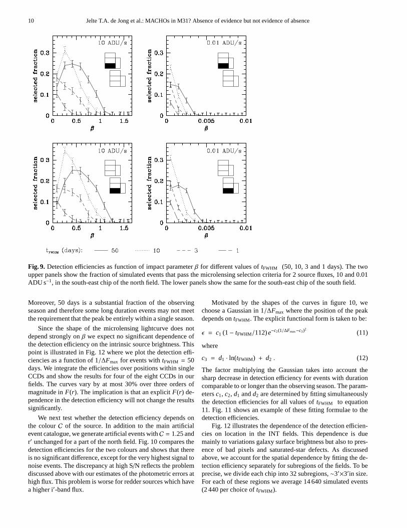
Fig. 9. Detection efficiencies as function of impact parameterβ for different values oftFWHM (50, 10, 3 and 1 days). The twoupper panels show the fraction of simulated events that passthe microlensing selection criteria for 2 source fluxes, 10 and 0.01ADU s−1, in the south-east chip of the north field. The lower panels show the same for the south-east chip of the south field.

Moreover, 50 days is a substantial fraction of the observingseason and therefore some long duration events may not meetthe requirement that the peak be entirely within a single season.

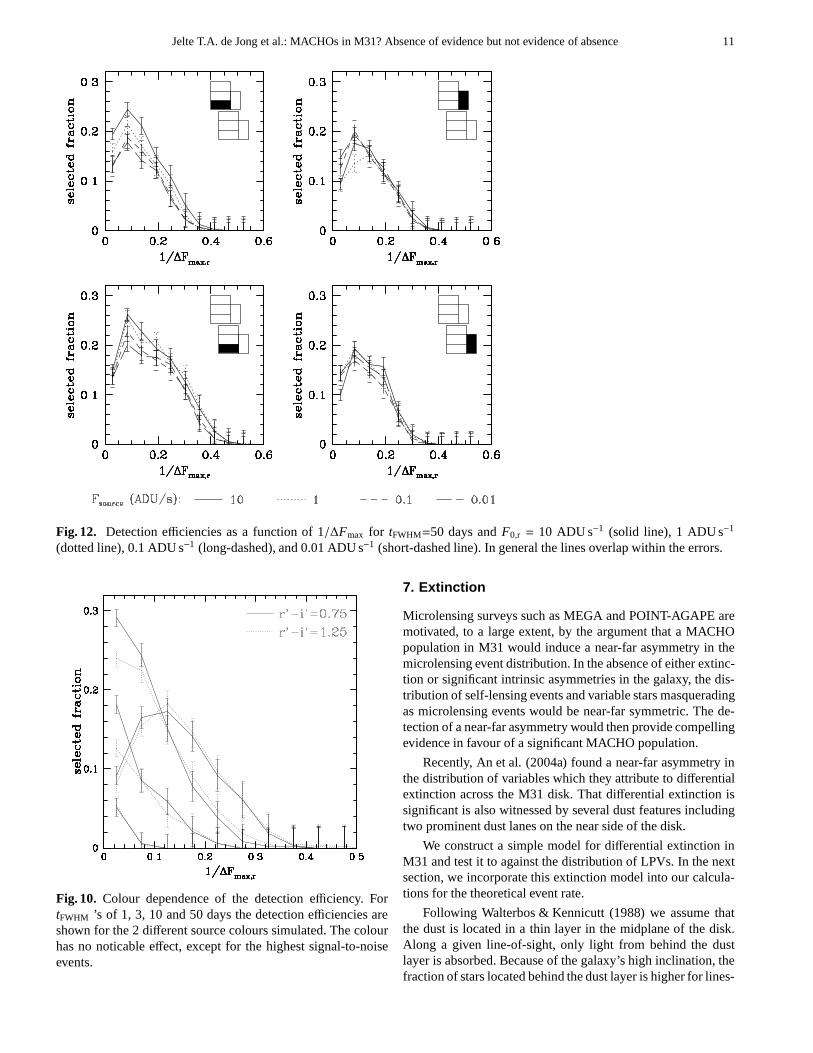
Since the shape of the microlensing lightcurve does notdepend strongly onβ we expect no significant dependence ofthe detection efficiency on the intrinsic source brightness. Thispoint is illustrated in Fig. 12 where we plot the detection effi-ciencies as a function of 1/∆Fmax for events withtFWHM = 50days. We integrate the efficiencies over positions within singleCCDs and show the results for four of the eight CCDs in ourfields. The curves vary by at most 30% over three orders ofmagnitude inF(r). The implication is that an explicitF(r) de-pendence in the detection efficiency will not change the resultssignificantly.

We next test whether the detection efficiency depends onthe colourC of the source. In addition to the main artificialevent catalogue, we generate artificial events withC = 1.25 andr′ unchanged for a part of the north field. Fig. 10 compares thedetection efficiencies for the two colours and shows that thereis no significant difference, except for the very highest signal tonoise events. The discrepancy at high S/N reflects the problemdiscussed above with our estimates of the photometric errors athigh flux. This problem is worse for redder sources which havea higher i′-band flux.

Motivated by the shapes of the curves in figure 10, wechoose a Gaussian in 1/∆Fmax where the position of the peakdepends ontFWHM. The explicit functional form is taken to be:

ǫ = c1 (1− tFWHM/112)e−c2(1/∆Fmax−c3)2(11)

where

c3 = d1 · ln(tFWHM) + d2 . (12)

The factor multiplying the Gaussian takes into account thesharp decrease in detection efficiency for events with durationcomparable to or longer than the observing season. The param-etersc1, c2, d1 andd2 are determined by fitting simultaneouslythe detection efficiencies for all values oftFWHM to equation11. Fig. 11 shows an example of these fitting formulae to thedetection efficiencies.

Fig. 12 illustrates the dependence of the detection efficien-cies on location in the INT fields. This dependence is duemainly to variations galaxy surface brightness but also to pres-ence of bad pixels and saturated-star defects. As discussedabove, we account for the spatial dependence by fitting the de-tection efficiency separately for subregions of the fields. To beprecise, we divide each chip into 32 subregions,∼3′×3′in size.For each of these regions we average 14 640 simulated events(2 440 per choice oftFWHM).


Fig. 12. Detection efficiencies as a function of 1/∆Fmax for tFWHM=50 days andF0,r = 10 ADU s−1 (solid line), 1 ADU s−1

(dotted line), 0.1 ADU s−1 (long-dashed), and 0.01 ADU s−1 (short-dashed line). In general the lines overlap within the errors.

Fig. 10. Colour dependence of the detection efficiency. FortFWHM ’s of 1, 3, 10 and 50 days the detection efficiencies areshown for the 2 different source colours simulated. The colourhas no noticable effect, except for the highest signal-to-noiseevents.

7. Extinction

Microlensing surveys such as MEGA and POINT-AGAPE aremotivated, to a large extent, by the argument that a MACHOpopulation in M31 would induce a near-far asymmetry in themicrolensing event distribution. In the absence of either extinc-tion or significant intrinsic asymmetries in the galaxy, thedis-tribution of self-lensing events and variable stars masqueradingas microlensing events would be near-far symmetric. The de-tection of a near-far asymmetry would then provide compellingevidence in favour of a significant MACHO population.

Recently, An et al. (2004a) found a near-far asymmetry inthe distribution of variables which they attribute to differentialextinction across the M31 disk. That differential extinction issignificant is also witnessed by several dust features includingtwo prominent dust lanes on the near side of the disk.

We construct a simple model for differential extinction inM31 and test it to against the distribution of LPVs. In the nextsection, we incorporate this extinction model into our calcula-tions for the theoretical event rate.

Following Walterbos & Kennicutt (1988) we assume thatthe dust is located in a thin layer in the midplane of the disk.Along a given line-of-sight, only light from behind the dustlayer is absorbed. Because of the galaxy’s high inclination, thefraction of stars located behind the dust layer is higher forlines-


Fig. 11. Detection efficiencies as a function of 1/∆Fmax fordifferent values oftFWHM. The symbols give the results of theMonte Carlo calculation for one chip. The lines correspond tothe fitting formula, equation 11.

of-sight on the near side of the disk than for those on the farside, as illustrated in Fig. 13. Therefore, even if the distributionof dust is intrinsically symmetric, extinction will have a greatereffect on the near side of the disk.

Based on these assumptions the observed intensity along aparticular line-of-sight is

Iobs = Ifront + Ibacke−τ (13)

whereIfront (Iback) is the intensity of light originating from infront of (behind) the dust layer andτ is the optical depth. Thisequation can be rewritten in terms of the total intrinsic intensity,Iintr, and the fractionx of light that originates from in front ofthe dust layer:

Iobs = xIintr + (1− x)Iintre−τ . (14)

The three unknowns in this equation,Iintr, x, ande−τ, dependon wavelength. Rewriting equation 14 for the B-band we have

e−τB =Iobs(B)/Iintr(B) − xB

1− xB. (15)

As a first approximation we assume thatIobs(I ) = Iintr(I ) sothat

e−τB =Iobs(B)/(CBI · Iobs(I )) − x

1− x(16)

whereCBI ≡ Iintr(B)/Iintr(I ) is the intrinsicI − B colour of thestellar population. An improved estimate ofIintr(I ) is obtainedby transforming the extinction factor from B to I via the stan-dard reddening law (Savage & Mathis 1979). The calculationis repeated several times

o13

FarNear

Fig. 13. Schematic representation of the line-of-sight throughthe M31 galaxy from an observer on earth. Because of the highinclination of M31, most of the light observed on the near sideof the disk is coming from behind the dust lanes.

Table 4.Disk and bulge parameters used to derivex, the frac-tion of light originating in front of the midplane of M31: thescalelength and scaleheight,hl andhz, for disk and bulge, andthe fraction of the total light coming from the bulge.

Disk Bulge Lb/(Lb + Ld)hl (kpc) hz (kpc) hl (kpc) hz (kpc)

B 5.8 0.3 1.2 0.75 0.39I 5.0 0.7 1.2 0.75 0.45

We approximatexB and xI from a simple model of thegalaxy wherein the intrinsic (i.e., three-dimensional) light dis-tribution η (x) for the disk and bulge are taken to be doubleexponentials. In cylindrical coordinates for M31, we have

ηi (x) = η0e−r/hiRe−z/hi

z (17)

where the superscripti denotes either the disk or bulge,η0

is a normalization constant, andhR andhz are the radial andvertical scale lengths, respectively. Different scale lengths areused for B and I because the two bands have different sen-sitivities to young and old populations of stars. Young starstend to lie closer to the disk midplane than old ones. Ourchoices for the parameters are given in Table 4. The val-ues of the disk scalelengths and the bulge-to-disk-ratios aretaken from Walterbos & Kennicutt (1988). The scalelengths forbulge are adapted from their de Vaucouleurs fit while the diskscaleheights are based on the distribution of different stellarpopulations in the Milky Way disk. The observablesIobs(I )andIobs(B) are from Guhathakurta et al. (2004) who cover a1.7×5 field centered on M31. We derive colour profiles fromtheir mosaics which are found to be similar to the profilesin Walterbos & Kennicutt (1988). The colour is approximatelyconstant within 30′′ and becomes bluer at larger radii.

Our I-band extinction map for M31 is shown in Fig. 14. Themajor dust lanes are clearly visible in the northern field and, asexpected, the derived extinction is much larger on the near sideof the galaxy than on the far side. The I-band attenuation is< 40% and reaches a maximum in the innermost dust lane anda few smaller complexes.

Our model almost certainly underestimates the effect ofextinction across the M31 disk. The approximationIobs(I ) ≃Iintr(I ) is a poor starting point in the limit of large opticaldepths. Forτ ≫ 1, most of the light in both B and I from be-hind the dust layer is absorbed and thereforeIobs(B)/Iobs(I ) ≃CBI. However substituting this result into equation 15 gives


< 0.6

0.6 - 0.7

0.7 - 0.8

0.8 - 0.9

0.9 - 1.0

== 1.0

major axis

Fig. 14. Calculated extinction map in the I-band. Extinction is clearly more severe on the near side of the disk. Note that thereare only a few small patches where the extinction factor rises above 40%.

exp(−τ) ≃ 1, an obvious contradiction. By the same token,if the dust is distributed in high-τ clumps, thenI andB wave-lengths will be absorbed by equal amounts given essentiallyby the geometric cross section of the clumps. Moreover, thethin-layer approximation tends to yield an underestimate of theextinction factor (Walterbos & Kennicutt 1988). Finally, scat-tering increases the flux observed towards the dust lanes andtherefore also leads one to underestimate the extinction factor.Some of these problems can be solved by using infrared datain the construction of the extinction map. In a future paper weplan to use 2MASS data in order to derive a more accuratemodel for differential extinction in M31.

We can use the distribution of variable stars in our surveyto test and refine the extinction model. The underlying assump-tion of this exercise is that the intrinsic distribution of vari-ables is the same on the near and far sides of the disk. Webegin by determining the periods of the variable stars usinga multi-harmonic periodogram (Schwarzenberg-Czerny 1996)suitably modified to allow for unevenly sampled data. A six-term Fourier series is then fit to each lightcurve yielding addi-

tional information such as the amplitude of the flux variations.Only variables with lightcurves that are well-fit by the Fourierseries are used.

We will use LPVs to test the extinction model becausethey generally belong to quite old stellar populations. This isan advantage because the majority of the microlensing sourcestars also belong to older populations which are more smoothlydistributed over the galaxy than younger variables such asCepheids. We select LPVs with periods between 150 and 650days and focus on two regions of our INT fields. One of these islocated on the near-side of the disk where extinction is expectedto be high while the other is located symmetrically about theM31 center on the far side. Fig. 15 shows the spatial distribu-tion of the LPVs. Since extinction reduces the amplitude of theflux variations and the average flux by the same factor we canstudy extinction by comparing the distributions in∆F for thenear and far sides. These flux variation distributions are shownin Fig. 16. For low∆F, where the shapes of the distributionsare dominated by the detection efficiency, results for the nearand far side agree. For high∆F, where the detection efficiency


Fig. 15.The distribution of the LPVs in M31 with the two sym-metrically placed regions used for the LPV amplitude analysisindicated. The northern field is located on the near side andcontains some of the most heavily extincted parts, the southernfield is on the far side and hardly affected by extinction. Theseregions are similar to N2 and S2 regions from An et al. (2004a),only adjusted to avoid the part of the southern INT field that isnot used in our analysis.

for variables approaches 100%, one finds a large discrepancybetween the near and far-side distributions.

To test whether this discrepancy is indeed due to extinctionwe transform the coordinates of LPVs on the far side to theirmirror image on the near side. The amplitude of the flux vari-ation is then reduced by the model extinction factor suitablytransformed from I to r′ (Savage & Mathis 1979). The new dis-tribution, shown in Fig. 16, is still significantly above thenear-side distribution at large∆F though it does provide a bettermatch than the original far-side distribution. The implication isthat our model underestimates extinction. To explore this pointfurther we consider models in whichτ is replaced bycτ wherec > 1. In Fig. 16, we show the distributions of the far side LPVsfor τ → 2τ (long-dashed line) andτ → 2.5τ (dot-dashed line).Apparently, the bright end of the (mirror) far-side distributionwith τ increased by a factor of 2.5 agrees with the bright end ofthe near-side distribution. We therefore conclude that ourorig-inal model does indeed underestimate the effects of extinction.In some places this will be stronger than in others, but over theprobed region the model underestimates extinction effectivelyby perhaps a factor of 2.5 inτ.

Fig. 16. Luminosity functions of LPVs in the 2 symmetri-cally placed regions. The far side flux distributions were scaledslightly to correct for small differences in area due to the gapsbetween the CCDs. The solid line is for the near side region andthe dotted for the uncorrected far side region. The short-dashed,long-dashed, and dot-dashed lines are far side distributions cor-rected for increasing levels of extinction.

8. Theoretical predictions

The detection efficiencies found in Sect. 6 allow us to predictthe number and distribution of events given a specific model forthe galaxy. Though M31 is one of the best studied galaxies, anumber of the parameters crucial for microlensing calculations,are not well-known. Chief among these are the mass-to-lightratios of the disk and bulge,(M/L)d and(M/L)b, respectively.The light distributions for these components are constrained bythe surface brightness profile while the mass distributionsof thedisk, bulge, and halo are constrained by the rotation curve andline-of-sight velocity dispersion profile. However, the mass-to-light ratios are poorly constrained primarily because the shapesof the disk and halo contributions to the rotation curve are simi-lar (e.g. van Albada et al. 1985). One can compensate for an in-crease in(M/L)d by decreasing the overall density of the halo.Stellar synthesis models (Bell & de Jong 2001), combined withobservations of the colour profile of M31, can be used to con-strain the mass-to-light ratios though these models come withtheir own internal scatter and assumptions. Another poorlycon-strained parameter is the thickness of the disk which affects thedisk-disk self-lensing rate.

In this section we describe theoretical calculations for theexpected number of events in the MEGA-INT survey. We con-sider a suite of M31 models which span a wide range of valuesin (M/L)d and (M/L)b. The dependence of the microlensingrate on other parameters is also explored.


8.1. Self-consistent models of M31

The standard practice for modeling disk galaxies is to choosesimple functional forms for the space density of the disk, bulge,and halo tuned to fit observational data. For microlensing calcu-lations, velocity distributions are also required. Typically, oneassumes that the velocity distribution for each of the compo-nents is isotropic, isothermal, and Maxwellian with a disper-sion given by the depth of the gravitational potential or, inthecase of the bulge, the observed line-of-sight velocity disper-sion. (But see Kerins et al. (2001) where the effects of velocityanisotry are discussed.) This approach can lead to a varietyofproblems. First, these “mass models” do not necessarily rep-resent equilibrium configurations, that is, self-consistent solu-tions to the collisionless Boltzmann and Poisson equations. Asystem initially specified by the model may well relax to a verydifferent state. Another issue concerns dynamical instability.Self-gravitating rotationally supported disks form strong bars.This instability may be weaker or absent altogether if the disk issupported, at least in part, by the bulge and/or halo. Therefore,models with very high(M/L)d are the most susceptible to barformation and can be ruled out.

In order to overcome these difficulties we use new,multi-component models for disk galaxies developed byWidrow & Dubinski (2005). The models assume axisymmetryand incorporate an exponential disk, a Hernquist model bulge(Hernquist 1990), and an NFW halo (Navarro et al. 1996).They represent self-consistent equilibrium solutions to the cou-pled Poisson and collisionless Boltzmann equations and aregenerated using the approach described in Kuijken & Dubinski(1995).

The phase-space distribution functions (DFs) for the disk,bulge, and halo (fdisk, fbulge, and fhalo respectively) are chosenanalytic functions of the integrals of motion. For the axisym-metric and time-independent system considered here, the an-gular momentum about the symmetry axis,Jz, and the energy,E, are integrals of motion. Widrow & Dubinski (2005) assumethat fhalo depends only on the energy whilefbulge incorporatesa Jz-dependence into the Hernquist model DF to allow for ro-tation. For both halo and bulge, the DFs are “lowered” as withthe King model (King 1966) so that the density goes to zero ata finite “truncation” radius. The disk DF is a function ofE, Jz,and an approximate third integral of motion,Ez, which corre-sponds to the energy associated with vertical motions of starsin the disk (Kuijken & Dubinski 1995).

Self-consistency requires that the space density,ρ, andgravitational potential,ψ, satisfy the following two equations:

ρ =

∫

d3v(

fdisk + fbulge+ fhalo

)

(18)

and

∇2ψ = 4πGρ . (19)

Self-consistency is achieved through an iterative scheme andspherical harmonic expansion ofρ andψ. Straightforward tech-niques allow one to generate an N-body representation suitablefor pseudo-observations of the type described below. The N-body representations also provide very clean initial conditions

for numerical simulations of bar formation and disk warpingand heating.

The DFs are described by 15 parameters which canbe tuned to fit a wide range of observations. In addition,one must specify mass-to-light ratios if photometric datais used. Our strategy is to compare pseudo-observations ofM31 with actual observational data to yield aχ2-statistic.Minimization of χ2 over the model parameter space – per-formed in Widrow & Dubinski (2005) by the downhill simplexmethod (see e.g. Press et al. 1992) – leads to a best-fit model.

Following Widrow & Dubinski (2005) (see, alsoWidrow et al. (2003) who carried out a similar exercisewith the original Kuijken & Dubinski (1995) models) weutilize measurements of the surface brightness profile,rotation curve, and inner (that is, bulge region) velocityprofiles. We use R-band surface brightness profiles for themajor and minor axes from Walterbos & Kennicutt (1988).(Widrow & Dubinski (2005) used the global surface bright-ness profile from Walterbos & Kennicutt (1988) which wasobtained by averaging the light distribution in ellipticalrings.The use here of both major and minor axis profiles should yielda more faithful bulge-disk decomposition.) The theoreticalprofiles are corrected for internal extinction using the modeldescribed in the previous section. In addition, a correction forGalactic extinction is included. We assume photometric errorsof 0.2 mag. We use a composite rotation curve constructedfrom observations by Kent (1989) and Braun (1991) thatrun from 2 to 25 kpc in galactocentric radius. Values anderror bars for the circular speed are obtained at intervals of10 arcmin ≃ 2.2 kpc using kernal smoothing (Widrow et al.2003). Finally, we use kinematic measurements from McElroy(1983) to constrain the dynamics in the innermost part of thegalaxy. We smooth his data along the minor axis to give valuesfor the line-of-sight stellar rotation and velocity dispersion at0.5 kpc and 1.0 kpc. The values at these radii are insensitiveto the effects of a central supermassive object and reflect thedynamics of the bulge stars with little disk contamination(McElroy 1983). An overallχ2 for the model is calculated bycombining results from the three types of data. Photometricand kinematic data are given equal weight; the circular rotationcurve measurements are weighted more heavily than the bulgevelocity and dispersion measurements. To be precise, we use

χ2 =1√

2

(

χ2sbp+

13χ2

disp+23χ2

rc

)

(20)

whereχ2sbp, χ

2bulge, andχ2

rc are the individualχ2-statistics forthe photometric, bulge kinematics, and rotation curve measure-ments.

In Fig. 17 we compare predictions for model A1 with ob-servations. Shown are the surface brightness profiles alongma-jor and minor axes and the circular rotation curve. Not shownis the excellent agreement between model and observationsfor the stellar rotation and dispersion measurements in thebulge region. Theχ2 statistic for this model is 1.06 (see Table5). This model was constructed assuming(M/L)d = 2.4 and(M/L)b = 3.6, values motivated by the stellar population syn-thesis models of Bell & de Jong (2001). Along the far side of


Fig. 17. Comparison of pseudo-observations of model A1 toreal observations.Upper panel:model surface brightness pro-files (solid lines) along the major and minor axis compared toobservations by Walterbos & Kennicutt (1988) (dots). For clar-ity the profiles are shifted down in steps of 2 magnitudes. Fromthe top down the profiles correspond to: SW major axis, NEmajor axis, SE minor axis (near side), and NW minor axis (farside).Lower panel:model rotation curve (solid line) and com-bined rotation curve from Kent (1989) and Braun (1991). Thethree lower lines correspond to the contributions to the rotationcurve of the bulge (dotted), disk (long dash) and halo (shortdash).

the minor axis, where the surface brightness profile is relativelyfree of extinction, theB−Rcolour is 1.8 in the bulge region and1.6 in the disk region Walterbos & Kennicutt (1988). A cor-rection for Galactic extinction brings these numbers down by0.18. Substituting into the appropriate formula from Table 1 ofBell & de Jong (2001) yield the mass-to-light ratios chosen forthis model.

In model A1, the scale height of the disk was fixed toa value of 1.0 kpc. Note that our model uses a sech2-lawfor the vertical structure of the disk. A sech2-scale height of1 kpc is roughly equivalent to an exponential scale height of0.5 − 0.7 kpc. The observations used in this study do not pro-vide a tight constraint on the scale height of the disk and so weappeal to observations of edge-on disk galaxies. Kregel et al.(2002) studied correlations between the (exponential) verticalscale height and other structural parameters such as the radialscale height and asymptotic circular speed in a sample of 34

edge-on spirals. Using these correlations we arrive at an ex-ponential scale height forM31 of 0.6 kpc with a fairly largescatter.

We also fix the disk truncation radius for this model to28 kpc which is at the high end of the range favoured inKregel et al. (2002). Lower values appear to be inconsistentwith the measured surface brightness profile. The remainingparameters for the disk, bulge, and halo DFs are varied in orderto minimizeχ2.

Table 5 outlines other models considered in this paper.Models B1-E1 explore the(M/L)b − (M/L)d plane. Theχ2 forthese models are generally quite low, a reflection of the modeldegeneracy mentioned above. In these models, disk and bulge“mass” are traded off against halo mass. Previous investigations(Widrow & Dubinski 2005) suggest that model E1 is unstableto the formation of a strong bar while the other models are sta-ble against bar formation or perhaps allow for a weak bar.

The aforementioned models used values for the extinctionfactor derived in Sect. 7. As discussed in that section, there area number of reasons to expect that this model underestimatesthe amount of extinction in M31. Indeed, our analysis of thenear-far asymmetry in LPVs favours a higher optical depth bya factor of 2.5, that is, the substitutione−τ → e−2.5τ. For thisreason, we consider a parallel sequence of models, A2-F2, withhigh extinction. Note that theχ2 for these models are as goodas if not better than those for the corresponding low-extinctionmodels.

8.2. Event rate calculation

The event rate is calculated by performing integrals over thelens and source distribution functions. The rate for lensestoenter the lensing tube of a single source is

d5R =fl(l l , vl)Ml

2REv⊥ dlldvl dβ (21)

wherefl is the DF for the lens population,l l is the observer-lensdistance (DOL in the language of equation 2),v⊥ is the trans-verse velocity of the lens with respect to the observer-sourceline-of-sight, andMl is the mass of the lens. In writing thisequation, we assume all lenses have the same mass.

For a distribution of sources described by the DFfs, equa-tion 21 is replaced by the following expression for the rate perunit solid angle

dRdΩ=

∫

fl(l l , vl)Ml

fs(ls, vs)(M/L)s Ls

2REv⊥

× dlldvl l2s dlsdvs dβ (22)

wherels is the observer-source distance,(M/L)s is the mass-to-light ratio of the source andLs is the source luminosity. (Forthe moment, we treat all sources as being identical.)

We perform the integrals using a Monte Carlo method. TheDFs are sampled at discrete points:

fp(lp, vp) =Σp

Np

Np∑

i=1

δ(lp − l i) δ(vp − vi) (23)


where p ∈ l, s, Σp is the surface density of either lensor source population, andNp is the number of points usedto Monte Carlo either lens or source populations. The nine-dimensional integral in equation 22 is replaced by a double sumand an integral overβ:

dRdΩ= Ssl

∑

i, j

∫ βu

0dβRi j (24)

where

Ssl =ΣlΣs

NlMlNsLs (M/L)s(25)

and

Ri j ≡ (2REv⊥)i j l2j . (26)

Note thatS depends on the line of sight densities of the lensand source distributions along with characteristics of thetwopopulations.Ri j depends on the coordinates and velocities ofthe lens and source (hence thei j subscripts). The sum is re-stricted to lens-source pairs withl l < ls. For each lens-sourcepair, the Einstein crossing time,tE,i j is easily calculated. Thedifferential event rate is then

d2RdΩdtE

= Ssl

∑

i, j

∫ βu

0dβRi jδ(tE,i j − tE) . (27)

8.3. Stellar and MACHO populations

The formulae in the previous section apply to the six lens-source combinations in our model: disk-disk, disk-bulge,bulge-disk, bulge-bulge, halo-disk, and halo-bulge. As writtenthe formulae assume homogeneous populations. For the diskand bulge populations, we modify equation 27 to include in-tegrals over the mass and luminosity functions as appropriate.We write the luminosity function (LF) as

dNdMR

= Ag(MR) . (28)

and the mass function as

dNdM = Bh(M,M0) (29)

where A and B are normalization constants andM0 is thelower bound for the mass function (MF). We take the func-tion g from Mamon & Soneira (1982) and the functionhfrom Binney & Merrifield (1998) (their equation 5.16) with thepower-law formdN/dM ∝M−1.8 extended toM0. A andB areevaluated separately for the disk and bulge populations. Inthecase of the disk, we assume that 30% of the mass is in the formof gas. The LF is normalized to giveL = L⊙ with the provisothatLs in equation 22 is given in solar units. To determine thenormalization constantB of the mass function, we write

Bh(M⊙,M0) =

(

dNdMV

dMV

dM

)∣

∣

∣

∣

∣

∣M=M⊙(30)

where the V-band LF is again from Mamon & Soneira (1982)and dMV/dM is from Kroupa et al. (1993). Equation 30 isevaluated at solar values for convenience. The relation( M

L

)

R=

∫

Bh(M,M0)MdM∫

Ag(MR)L(MR)dMR

(31)

can then be solved forM0. Thus, a disk with highM/L containsmore low-mass stars than a disk with lowM/L.

For simplicity, and because we lack a model for whatMACHOs actually are, we assume all MACHOs have the samemass,MM that is

dNdM = δ (M−MM) . (32)

8.4. Theoretical prediction for the number of events

Recall that the efficiency ǫ is written as a function oftFWHM

and∆Fmax. (The efficiency also depends on the line of sight.)These quantities are explicit functions ofβ, Fr , andtE. Thus,the expected number of events per unit solid angle is

dEdΩ= E A BSls

∑

i, j

∫ βu

0dβ

∫

dMRg (MR)

×∫

dMlh (M,M0)Ri j ǫ (tFWHM, ∆F) (33)

whereE is the overall duration of the experiment. Our surveycovers four half-year seasons and so, with our choice of unitsfor ǫ anddR/dΩ, we haveE = 2.

The number of events expected in each of the 250 bins usedfor the extinction calculation and labelled by “k” is

Ek = ∆Ω

(

dEdΩ

)

k

(34)

where∆Ω = 9 arcmin2 is the angular area of a bin.Ek car-ries an additional label (suppressed for notational simplicity)which denotes the lens-source combination. The total numberof events isE = ∑Ek.

8.5. Binary lenses

Our microlensing selection criteria are based on the assump-tion that the lenses are single point-mass objects. However,at least half of all stars are members of multiple star sys-tems. Microlensing lightcurves for a lens composed of two ormore point masses can deviate significantly from the standardlightcurve (Schneider & Weiss 1986) and may therefore escapedetection. The deviations are strongest when the source crossesor comes close to the so-called caustics, positions in the sourceplane where the magnification factor is formally infinite. (Theactual magnification factor is finite due to the finite size ofthe source.) The size of the caustic region is largest when theseparation of the components of the lens is comparable to theEinstein radius corresponding to the total mass (equation 2).Mao & Paczynski (1991) estimated that∼10% of microlensingevents towards the bulge of the Milky Way (mainly self-lensing


events) should show strong binary characteristics. Since theEinstein radius for bulge-bulge self-lensing toward the MilkyWay and M31 are comparable, we can expect a similar 10% ef-fect in our survey. That is, the calculated theoretical predictionsfor self-lensing are revised downward by∼ 10%.

8.6. Results

Table 5 presents the theoretical predictions for the total numberof events expected in the MEGA-INT four-year survey. Theresults are given for both self-lensing (Eself) and halo lensing(Ehalo). The values quoted forEhalo assume 100% of the halo isin the form of MACHOs. In other words, these values shouldbe multiplied by the MACHO halo fraction in order to get theexpected number of events for a MACHO component. We notethat lensing by the Milky Way halo is not included in theseresults. This possible contribution is expected to be small, sincethe number of microlensing events from a 100% MW halo isa few times lower than for a 100% M31 halo (Gyuk & Crotts2000; Baillon et al. 1993) for MACHO masses around 0.5M⊙.

We also consider the near-far asymmetry for self and halolensing. In Fig. 18, we show the cumulative distribution ofevents for self and halo lensing as a function of the distancefrom the major axis,s. We takes to be positive on the far sideof the disk. For this plot, we choose model A1 but since the dis-tributions are normalized to give 14 total events, the differencebetween the models is rather inconsequential. We see that bothself and halo lensing models do a good job of describing theevent distribution in the inner 0.2. The halo distribution doesa somewhat better job of modelling the three events betweens = 0.2 and s = 0.3. Neither halo nor self lensing modelspredict anywhere near two event fors> 0.35.

To further explore the distribution, we define the asymme-try parameterA:

A =∑Ek · sk

E . (35)

In Table 5 we give values forAself andAhalo. We also pro-vide an averageAave which assumes that MACHOs make upthe shortfall between the expected number of events and theobserved value of 14. In cases where the expected number ofevents is greater than 14, we setAave = Aself. The asymmetryparameter for the 14 candidate events isAdata= 0.125.

The general trend, in terms of total expected number ofevents, is that as the mass-to-light ratios are increased,Eself

increases andEhalo decreases. There are counter examples. Inmodel C1, the(M/L)b (as compared with model A1) leads to aless massive disk and lowerEself. Recall that for each choice ofmass-to-light ratios, the remaining parameters are adjusted tominimizeχ2. The process can lead to rather complicated inter-dependencies between the model parameters. The self-lensingrate decreases with decreasinghz as illustrated with model F1.The self-lensing rate is generally reduced in the high extinctionmodels relative to the low extinction ones. Finally we see thatthe halo event rate decreases with increasing MACHO mass.Models G and H illustrate this point and span the range inMM

identified by Alcock et al. (2000) as the most probable massrange for Milky Way MACHOs.

Fig. 18.Cumulative event distribution as a function of distancefrom the major axis (in degrees). Shown are the data (dots),self-lensing distribution (solid line), and halo-lensingdistribu-tion (dotted line). Both self- and halo-lensing lines are scaledto give a total of 14 events.

Fig. 19.Cumulative microlensing event distribution as a func-tion of timescale. The line and point-types are the same as inFig. 18.

The timescale distribution is easily calculated using themethod outlined in the previous section. Essentially, one calcu-latestFWHM for each lens-source pair in the Monte Carlo sum.In Fig. 19 we show the cumulative timescale distribution of ourcandidate microlensing event sample and model A1. In con-structing the curves for self and halo lensing, we have scaledthe distributions to give a total of 14 events.


Table 5. Results of the microlensing modeling using self-consistent M31 models. In the first columns some model parametersand the combinedχ2 are listed. The remaining columns contain the predicted number of events due to self-lensing (Esel f), due tohalo-lensing (Ehalo), the asymmetry of the self-lensing (Asel f), of the halo-lensing (Ahalo), and of the combination of both (Aave).The number of self-lensing eventsEsel f has been corrected for the fact that∼10% of the events will show strong binary effectsand therefore be selected against. The microlensing event rate due to the haloEhalo is for a 100% MACHO halo, i.e. all of thehalo mass is assumed to be in the MACHOs. For calculating the combined self- and halo-lensing asymmetry parameterAave asmaller fraction of the halo mass is assumed to be in MACHOs, namely the amount necessary to make up the difference, if any,betweenEsel f and the observed number of 14 candidate events. The disk scale heightshz aresech2 scale heights. The upper, lowextinction part of the table contains models with internal extinction values as derived in section 7, while the lower, high extinctionpart contains models with increased extinction, as motivated by our analysis of the LPV amplitudes.

Low extinction

Models withm=0.5 M⊙ andhz=1.0 kpc(M/L)d (M/L)b χ2 Eself Ehalo Aself Ahalo Aave

A1 2.4 3.6 1.06 14.2 30.9 0.037 0.086 0.037B1 2.4 2.9 1.17 13.4 31.5 0.031 0.085 0.033C1 2.4 4.3 1.02 13.1 29.6 0.039 0.092 0.043D1 1.8 2.4 1.34 11.3 35.5 0.031 0.082 0.041E1 3.6 4.4 1.03 15.8 24.6 0.030 0.091 0.030

Models with (M/L)d=2.4 and (M/L)b=3.6hz MM χ2 Eself Ehalo Aself Ahalo Aave

F1 0.5 0.5 1.10 12.5 30.7 0.037 0.084 0.042G1 1.0 0.1 1.06 14.2 43.1 0.037 0.088 0.037H1 1.0 1.0 1.06 14.2 25.9 0.037 0.085 0.037

High extinction

Models withMM = 0.5M⊙ andhz=1.0 kpc(M/L)d (M/L)b χ2 Eself Ehalo Aself Ahalo Aave

A2 2.4 3.6 0.99 12.4 28.6 0.052 0.095 0.057B2 2.4 2.9 1.08 12.2 32.6 0.046 0.094 0.052C2 2.4 4.3 0.99 14.5 29.6 0.056 0.098 0.056D2 1.8 2.4 1.23 10.3 34.5 0.045 0.095 0.058E2 3.6 4.4 1.04 14.2 22.8 0.046 0.105 0.046

Models with (M/L)d=2.4 and (M/L)b=3.6hz MM χ2 Eself Ehalo Aself Ahalo Aave

F2 0.5 0.5 1.06 11.2 30.5 0.052 0.095 0.061G2 1.0 0.1 0.99 12.4 39.1 0.052 0.098 0.057H2 1.0 1.0 0.99 12.4 23.8 0.052 0.093 0.057

9. Discussion

The numbers expected for events due to self-lensing across themodels probed in Table 5 fall within the narrow range of 10-16. The relative insensitivity ofEself to changes in the mass-to-light ratios is a result of our approach to constructing models;changes in(M/L)b and(M/L)d are compensated by changes inthe structural parameters of the disk, bulge, and halo so as tominimizeχ2 for the fit to the rotation curve and surface bright-ness data. Consider models D1 and E1. The mass-to-light ratiosdiffer by a factor of∼ 2 whileEself differs by only a factor of1.4; with the lowM/L values in model D1, the rotation curvedata drive up the disk and bulge luminosity distributions attheexpense of a poorer fit for the photometric data. A balance isstruck and the net result is that the change inEself is signifi-cantly smaller than what one might expect.

The analysis of the first three seasons of INT data bythe POINT-AGAPE collaboration (Calchi Novati et al. 2005)provides a cautionary tale in this regard. They presentsix high quality, short duration microlensing candidateswith one of these events attributed to M32-M31 lensing.Calchi Novati et al. (2005) also model the detection efficiencyand calculate number of expected self and halo-lensing eventsfor a variety of M31 models. In all of their models, the num-ber of events for self lensing is predicted to be less than∼ 1.5.Since this number is significantly less than the observed num-ber, they conclude that some of the events are due to MACHOsand estimate that the MACHO halo fraction is at least 20%.

Calchi Novati et al. (2005) use the model from Kerins et al.(2001) but allow the disk and bulge mass-to-light ratios andbulge dispersion to vary. Herein lies the problem. Kerins etal.(2001) choose(M/LB) = 4 and 9 for the disk and bulge, re-spectively with the structural parameters for the disk, bulge,


and halo chosen to fit the observed surface brightness profileand rotation curve. The reference model in Calchi Novati et al.(2005) uses the same structural parameters for the three com-ponents but takes(M/LB)b = 3. For fixed bulge “light”, thischange in the mass-to-light ratio implies a rotation curve thatfalls short of the data at small radii as illustrated in the upperpanel of Fig. 20. The result is that Calchi Novati et al. (2005)have underestimated the self-lensing rate.

Calchi Novati et al. (2005) argue that the evidence is insen-sitive to large changes in the mass-to-light ratios of the disk andbulge. In their Table 11 they explore the dependence of the self-lensing rate on disk and bulge mass-to-light ratios. The numberof events expected for the reference model is 0.72. The numberincreases to 1.1 when the disk mass-to-light ratio is increasedto 9 but this model also gives a poor fit to the rotation curve(see middle panel of Fig. 20). They also find that the expectednumber of self-lensing events increases to 1.5 when the bulgemass-to-light ratio is increased to 8 and this model does pro-vide a good fit to the rotation curve. At first glance, an increasein the self-lensing rate by a factor of two over the referencemodel makes sense since this is approximately the same factorby which the bulge mass is increased. However, this line-of-reasoning ignores dynamical considerations which demand thatthe velocity dispersion increase roughly as the square rootofthe mass. We have created self-consistent models that closelyapproximate the models in Table 11 of Calchi Novati et al.(2005) and find that the increase in the expected number of self-lensing events is roughly a factor of four when the bulge mass-to-light ratio is increased from 3 to 8. Thus, for their heavybulge model, we expect 3 events from self lensing which is notsignificantly different from the observed number, 5.

One final note. The choice of 0.3 kpc for thesech2 scaleheight is small by perhaps a factor of 3 if M31 is a typical spi-ral galaxy as represented in the survey by Kregel et al. (2002).Thickening the disk increases the disk-disk self-lensing rate.

For our models, the number of events due to self-lensingis consistent with the total number of events observed but notinconsistent with a significant MACHO fraction for the halo ofM31. We can make this statement more quantitative by treatinghalo events as a Poisson process with background due to self-lensing and employing the approach of Feldman & Cousins(1998). We letn be the number of observed events consistingof MACHO events with meanfEhalo, where f is the MACHOfraction, and a background due to self-lensing with knownmeanEself. For this analysis, we ignore the background dueto variables and background supernovae. The probability dis-tribution function

P (n| f ) = ( fEhalo+ Eself)n exp

[− ( fEhalo+ Eself)]

/n! . (36)

To obtain confidence intervals forf :

1. CalculateP (n| f ) for N values of f ∈ 0, 1 and sort fromhigh to low. The maximum ofP defines the most probablevalue of f . The values ofP are normalized so that the sumof all sampled values ofP is 1.

2. Accept values off starting from the highest value ofP un-til the sum ofP exceeds the desired confidence level. Thelargest and smallest values of acceptedf define the confi-dence interval.

Fig. 20.Comparison of observed rotation curve with the rota-tion curves based on the models used in Calchi Novati et al.(2005). Upper panel: the default model.Middle panel: theheavy disk model.Lower panel:the heavy bulge model. Theline types and observational data are the same as in Fig. 17.

In Table 6 we provide most probable values off and 95%confidence intervals for all of the models in Table 5. We providethese values both for the case of the full sample of 14 observedcandidate events (n=14), as well as for the case of 11 observedevents (n=11), for reasons discussed below.

We next turn to the distribution of events across the M31disk as represented by the asymmetry parameters. From Table5 we see thatAself < Ahalo < Adata. The (weak) asymmetry inthe self-lensing distribution is due to extinction. Note that thevalues are significantly belowAdataeven for the high extinctionmodels.

The asymmetry parameter for the halo is signicantly higherthan that for self-lensing events and close to, though stillbe-low, Adata. However, the asymmetry parameter for combina-tions of self and halo lensing are well belowAdata. Evidently,the distribution of candidate events is difficult to explain withany reasonable combination of self and halo lensing.

The large asymmetry in the data is due, for the most part,to events 11, 13, and 14 (see Table 7). It is therefore worthconsidering alternative explanations for these events. Asarguedin Paulin-Henriksson et al. (2002), the lens for event 11 likelyresides in M32 and since we have not included M32 in ourmodel, this event should be removed from the analysis. Doingso leads to a modest reduction inAdata.

Events 13 and 14 may be more difficult to explain. Formodel A1, the predicted number of self-lensing events withs>s(event 18) is 0.005 while the predicted number of MACHO


events in the same range ins is 0.14f . Thus, the probability ofhaving two events either from self or halo lensing is exceed-ingly small, unless the halo fraction is very large. However,since some contamination by variable stars of our sample cannot be excluded, one or both of these events may be a variablestar. We note, for example, that event 13 has the lowest S/N inour sample. The probability of having one event for MACHOlensing with f = 0.20 is∼ 3%, small, but not vanishingly so.

A closer inspection of the model is also warranted.Recall that our models assume axisymmetry whereas M31exhibits a variety of non-axisymmetric features such as diskwarping. This point is illustrated in the isophotal map byHodge & Kennicutt (1982). From the map, one finds that event13 lies on the B=24 (R=22.6) contour while model A1 predictsR=23.5. Thus, the model may in fact underestimate the surfacebrightness of the disk by a factor of 2, and hence the disk-diskself-lensing rate by a factor of 4. (The reason for the discrep-ancy is not completely clear. The contours on the far side doappear to be “boxier” than those predicted by the model.)

It is interesting to note that events 13 and 14 are coinci-dent with the location of the giant stellar stream discoveredby Ibata et al. (2001). This stream runs across the southernINT field, approximately perpendicular to the major axis andover M32. Indeed, M32 may be the progenitor of the stream(Merrett et al. 2003). The average V-band surface brightness ofthe stream isΣV ≈ 30± 0.5 mag arcsec−2 (Ibata et al. 2001)but this is measured far from the projected positions of events13 and 14. The surface brightness of the stream might be sig-nificantly higher near the position of M32. Perhaps the mostconservative statement one can make about the stream is thatitis not bright enough to distort the contours near events 13 and14, that is, it cannot be brighter than the disk at these radii. Themicrolensing event rate due to stars in the stream is of courseenhanced relative to the rate for self-lensing by the ratio of thedistance from the stream to the disk and the thickness of thedisk, that is, by a factor of∼ 20. The stream-disk lensing ratemight be further enhanced if the stars in the stream have a largeproper motion relative to the disk. These arguments suggestthat the number of stream-disk events in the vicinity of M32might be 0.03− 0.1; perhaps high enough to explain one event.

Fig. 21 provides a summary of our results with respect tothe expected number of events and the asymmetry parameter.The points with error bars represent the data for the 4 casesconsidered in Table 7. The solid circles and lines correspondto the high extinction case; the open circles and dotted linescorrespond to the low extinction case. The circles assume pureself lensing while the lines trace out the values for increasingMACHO fraction with the tick-mark indicating the position off = 0.2. Once again, we see that the asymmetry parameter forthe data is higher than that for any of the models. Removingevents 13 and 14 does improve the situation as does increasingthe optical depthτ; the asymmetry remains a little higher butconsistent with the models.

10. Conclusions

This paper presents the analysis of four seasons of M31 ob-servations at the INT, a subset of the MEGA survey of M31.

Table 6.Most probable value and 95% confidence limits for theMACHO halo fraction f from the Feldman & Cousins (1998)analysis, for the full sample and the case without candidateevents 11, 13, and 14.

14 events 11 eventsmodel fbest conf. interval fbest conf. intervalA1 0. [0,0.28] 0. [0.,0.21]B1 0.02 [0,0.29] 0. [0.,0.22]C1 0.03 [0,0.32] 0. [0.,0.24]D1 0.08 [0,0.30] 0. [0.,0.22]E1 0. [0,0.32] 0. [0.,0.25]F1 0.05 [0,0.32] 0. [0.,0.24]G1 0. [0,0.20] 0. [0.,0.15]H1 0. [0,0.34] 0. [0.,0.25]A2 0.06 [0.,0.35] 0. [0.,0.25]B2 0.06 [0.,0.31] 0. [0.,0.23]C2 0. [0.,0.29] 0. [0.,0.22]D2 0.11 [0.,0.33] 0.02 [0.,0.24]E2 0. [0.,0.39] 0. [0.,0.29]F2 0.09 [0.,0.35] 0. [0.,0.26]G2 0.04 [0.,0.25] 0. [0.,0.18]H2 0.07 [0.,0.42] 0. [0.,0.31]

Table 7. Observed number of events and the asymmetry oftheir spatial distribution, shown for the full sample of 14 eventsand for cases where the probable M32 event (11) and candi-date events 13 and 14 are ignored. The quoted errors are 1σ

errors, determined with the bootstrap method. Also shown isthe asymmetry for the long-period variable stars (LPVs).

Events used Edata Adata

Full sample 14 0.125± 0.046without 11 13 0.120± 0.049without 13, 14 12 0.076± 0.034without 11, 13, 14 11 0.066± 0.034LPVs 20,864 0.071± 0.001

The observations were carried out to search for MACHOs inthe halo of M31. Our fully automated search algorithm iden-tified 14 candidate microlensing events from over 105 variablesources. Three of the candidates were previously unpublished.The spatial and timescale distributions are consistent with mi-crolensing.

The core of this paper is the comparison of this candidateevent sample with a calculation of the expected number ofevents from self and halo lensing. This calculation breaks intothree parts: a model for the extinction across the M31 disk; amodel for the detection efficiency; and a suite of self-consistentdisk-bulge-halo models for M31.

The results with regard to the fundamental question ofwhether there is a significant MACHO fraction in the halo areinconclusive. Based on the total number of events, we find thatthe most probable MACHO halo fractionf varies between 0and 0.1 depending on the model. Our event rate analysis is con-sistent with a total absence of MACHOs as the confidence in-tervals for all of our models includef = 0. On the other handwe can not exclude some MACHO component, since the con-


10 15 20 250.02

0.04

0.06

0.08

0.1

0.12

Fig. 21.Asymmetries and event numbers for data and models.The points with error bars on the left showE andA for thesample of candidate events and the subsamples listed in table7. The solid lines correspond to the high and the dotted linestothe low extinction models from table 5. The dots are the pureself-lensing points, with the MACHO mass fraction increasingalong the line. MACHO fractions of 20% are indicated withvertical lines.

fidence intervals extend typically up tof = 0.25 and even upto f = 0.4 for a few models.

The spatial distribution of the candidate events is highlyasymmetric and does seem to favor a MACHO component.However, for different reasons it is questionable whether the3 candidate events that largely determine the asymmetry signalshould be used in this analysis. Thus, we conclude that bothfrom the observed number of events, and from their spatial dis-tribution we find no compelling evidence for the presence ofMACHOs in the halo of M31.

Acknowledgements.We would like to thank Raja Guhathakurta andPhil Choi for making their M31 map available to us and StephaneCourteau for useful conversations. We also thank all observers whohave performed the observations for this survey and the ING staff.Support is acknowledged from STScI (GO 10273) and NSF (grants0406970 and 0070882). JdJ and KK thank the LKBF for travel sup-port.

References

Afonso, C., Albert, J. N., Andersen, J., et al. 2003, A&A, 400,951

Alcock, C., Allsman, R. A., Alves, D. R., et al. 2000, ApJ, 542,281

An, J. H., Evans, N. W., Hewett, P., et al. 2004a, MNRAS, 351,1071

An, J. H., Evans, N. W., Kerins, E., et al. 2004b, ApJ, 601, 845An, J. H., Evans, N. W., Kerins, E., et al. 2004c, ApJ, 601, 845

Baillon, P., Bouquet, A., Giraud-Heraud, Y., & Kaplan, J. 1993,A&A, 277, 1

Baltz, E. A., Gyuk, G., & Crotts, A. 2003, ApJ, 582, 30Baltz, E. A. & Silk, J. 2000, ApJ, 530, 578Bell, E. F. & de Jong, R. S. 2001, ApJ, 550, 212Belokurov, V., An, J., Evans, N. W., et al. 2005, MNRAS, ???Bertin, E. & Arnouts, S. 1996, A&AS, 117, 393Binney, J. & Merrifield, M. 1998, Galactic astronomy

(Galactic astronomy / James Binney and MichaelMerrifield. Princeton, NJ : Princeton University Press,1998. (Princeton series in astrophysics) QB857 .B522 1998($35.00))

Braun, R. 1991, ApJ, 372, 54Calchi Novati, S., Jetzer, P., Scarpetta, G., et al. 2003, A&A,

405, 851Calchi Novati, S., Paulin-Henriksson, S., An, J., et al. 2005,

subm., astro-ph/0504188Crotts, A. P. S. 1992, ApJL, 399, L43Darnley, M. J., Bode, M. F., Kerins, E., et al. 2004, MNRAS,

353, 571de Jong, J. T. A., Kuijken, K., Crotts, A. P. S., et al. 2004, A&A,

417, 461Feldman, G. J. & Cousins, R. D. 1998, Phys. Rev. D, 57, 3873Gondolo, P. 1999, ApJL, 510, L29Gould, A. 1996, ApJ, 470, 201Guhathakurta, P., Choi, P. I., & Raychaudbury, S. 2005, in prepGyuk, G. & Crotts, A. 2000, ApJ, 535, 621Hernquist, L. 1990, ApJ, 356, 359Hodge, P. W. & Kennicutt, R. C. 1982, AJ, 87, 264Ibata, R., Irwin, M., Lewis, G., Ferguson, A. M. N., & Tanvir,

N. 2001, Nature, 412, 49Kent, S. M. 1989, AJ, 97, 1614Kerins, E., Carr, B. J., Evans, N. W., et al. 2001, MNRAS, 323,

13King, I. R. 1966, AJ, 71, 64Kregel, M., van der Kruit, P. C., & de Grijs, R. 2002, MNRAS,

334, 646Kroupa, P., Tout, C. A., & Gilmore, G. 1993, MNRAS, 262,

545Kuijken, K. & Dubinski, J. 1995, MNRAS, 277, 1341Lasserre, T., Afonso, C., Albert, J. N., et al. 2000, A&A, 355,

L39Mamon, G. A. & Soneira, R. M. 1982, ApJ, 255, 181Mao, S. & Paczynski, B. 1991, ApJL, 374, L37McElroy, D. B. 1983, ApJ, 270, 485Merrett, H. R., Kuijken, K., Merrifield, M. R., et al. 2003,

MNRAS, 346, L62Navarro, J. F., Frenk, C. S., & White, S. D. M. 1996, ApJ, 462,

563Paczynski, B. 1986, ApJ, 304, 1Paulin-Henriksson, S., Baillon, P., Bouquet, A., et al. 2002,

ApJL, 576, L121Paulin-Henriksson, S., Baillon, P., Bouquet, A., et al. 2003,

A&A, 405, 15Press, W. H., Teukolsky, S. A., Vetterling, W. T., & Flannery,

B. P. 1992, Numerical recipes in C. The art of scientific com-puting (Cambridge: University Press, —c1992, 2nd ed.)

Riffeser, A., Fliri, J., Bender, R., Seitz, S., & Gossl, C. A. 2003,


ApJL, 599, L17Savage, B. D. & Mathis, J. S. 1979, ARA&A, 17, 73Schneider, P. & Weiss, A. 1986, A&A, 164, 237Schwarzenberg-Czerny, A. 1996, ApJL, 460, L107+Tomaney, A. B. & Crotts, A. P. S. 1996, AJ, 112, 2872Uglesich, R. R., Crotts, A. P. S., Baltz, E. A., et al. 2004, ApJ,

612, 877van Albada, T. S., Bahcall, J. N., Begeman, K., & Sancisi, R.

1985, ApJ, 295, 305Walterbos, R. A. M. & Kennicutt, R. C. 1988, A&A, 198, 61Widrow, L. M. & Dubinski, J. 2005, ApJ., in pressWidrow, L. M., Perrett, K. M., & Suyu, S. H. 2003, ApJ, 588,

311

Appendix A: Candidate event lightcurves

On the following pages, for each of the 14 candidate microlens-ing events in our sample, the r′ and i′ lightcurves and thumb-nails taken from the difference centered on the event positionsare shown, together with a short discussion. Apart from the INTr′ and i′ data, KP4m R and I data points are also plotted in thelightcurves. The fits shown are however the fits done to onlythe INT data.


MEGA-ML-1

Located close to the center of M31, this event has a rather noisybaseline. Apart from the background of very faint variablesthere are some variable sources clearly visible in the differenceimages. As can be seen in the thumbnails in figure A.1(b) abright variable is located just a few pixels from the position ofthe candidate event. Another, fainter variable is seen at a simi-lar distance above and to the left. The other variable sources arefurther away and should have no influence on the photometry.

MEGA-ML-2

This candidate event is located very close to MEGA-ML-1 andtherefore has the same problems connected to being close thecenter of M31. In the thumbnails of days 94, 754, and 1208we see a variable source a few pixels to the left of the eventposition. This variable is brighter in r′ than in i′, which causesthe r′ baseline to be the most noisy.

MEGA-ML-3

This candidate event is also located close to the M31 center.In figure 6 we already demonstrated that a very faint variablesource is positioned∼0.25′′away from this candidate event. Inthe i′ thumbnails another variable is visible just above and tothe right of the event. This variable has a bright episode be-tween days 440 and 480, causing the bump in the baseline inthe i′ lightcurve.

MEGA-ML-7

By far the brightest event in our sample, the thumbnails ofMEGA-ML-7 show a very bright residual close to the peakcenter. Since the peak occurs during the first season, some ofthe exposures used for creating the reference image containeda significant amount of the magnified flux, so that the base-line lies at a negative difference flux. There are some variablesnearby, but none of them are close or bright enough to signif-icantly influence the photometry. The distance to the centerofM31 is also quite large (∼22′), reducing the background of faintvariable sources. As pointed out by Paulin-Henriksson et al.(2003), there are some systematic deviations from the best fitmicrolensing model. An et al. (2004c) find that this anomalycan be explained by a binary lens.

MEGA-ML-8

This near side event is located∼23′ from the center of M31.A variable that is particularly bright in i′ is situated about2.4′′ NW of the candidate event, but should not have muchof an effect on the photometry. The baselines of the lightcurvesindeed look stable and well-behaved.

MEGA-ML-9

Peak coverage is poor for this candidate event, but the baselinesare stable. The thumbnails show quite a lot of faint variables,

two of which are located very close, approximately 1′′ to theleft of the event position, accounting for the noise in the i′ base-line that is higher than in the r′ lightcurve.

MEGA-ML-10

This event is a beautiful example of a combined lightcurve withKP4m and INT data. Peak coverage in INT i′ is poor, but theKP4m I data points follow the fit (derived only from INT data)very well. A fairly bright variable is situated slightly above andto the right of the event position and there is a hint of a veryfaint variable about 1′′ to the left. Although the INT baselinein i′ is noisy, the r′ and both KP4m R and I lightcurves show anvery stable and well-behaved baseline.


figapp01a.gif

Fig. A.1. (a)Event 1: lightcurves. The two upper panels show the full r′ and i′ lightcurves of the microlensing event. In the lowerleft corner are zooms on the peak region. In the lower right corner the r′ flux is plotted versus the i′ flux; if the colour is constant,the points should lie on a straight line. Also drawn is the best fit microlensing model. The solid circles are points from the INTdata, the open circles are from the KP4m data. The start of theINT survey, August 1st 1999, is used as the zeropoint for thetimescale.

figapp01b.jpg

Fig. A.1. (b) Event 1: thumbnails. The two upper rows of thumbnails show are taken from r′ and i′ difference images during thepeak of the candidate event. Selected thumbnails from the baseline are also shown in the two bottom rows. Each thumbnail is30×30 pixels or 10×10′′ in size.

figapp02a.gif

Fig. A.2. (a)Event 2: lightcurves. See caption of A.1(a).

figapp02b.jpg

Fig. A.2. (b) Event 2: thumbnails. See caption of A.1(b).


figapp03a.gif


figapp03b.jpg


figapp04a.gif


figapp04b.jpg


figapp05a.gif



figapp05b.jpg


figapp06a.gif


figapp06b.jpg


figapp07a.gif


figapp07b.jpg



MEGA-ML-11

A high signal-to-noise event with a good fit and stable base-line. There is some noise in the i′ baseline, caused by the vari-able source that is visible in the thumbnails of days 6 and 756at ∼1.3′′ above the event position. During the fourth observ-ing season a few bad columns were lying exactly on top of theevent position, so that there is only 1 INT data point available.However, the KP4m data show that the baseline remains flateverywhere.

MEGA-ML-13

This candidate event has the lowest signal-to-noise of our sam-ple. It is situated far out in the far side of the disk at∼31′ fromthe center of the galaxy and the relatively low galaxy back-ground makes it possible to detect these kind of faint events.Due to the y-axis scale the i′ the baseline looks quite noisy,but it is in fact not significantly more so than for other candi-date events. The thumbnails of days 398 and 520 show that theclosest variable source is located∼1.4′′ below and to the leftof the event, which explains the scatter in the i′ baseline.

MEGA-ML-14

At ∼35.5′ from the M31 center, this candidate event is the mostfar out in the disk of all events in our sample. The i′ photometryof this candidate event is compromised by the variable sourceat∼1.3′′. From the i′ thumbnails one can also see that the eventlies at the edge of a fringe, making the background in the lowerhalf of the thumbnails brighter than in the upper half. This canalso cause some extra scatter in the photometry. Overall, how-ever, the microlensing fit is very good and both INT and KP4mlightcurves show a stable baseline.

MEGA-ML-15

This event is again located close to the center of M31 and pre-sumably has a strong background of faint variable sources. Inthe thumbnails also several variables are visible very close tothe event position, both in r′ and in i′. The lightcurve base-lines are rather noisy because of this, but show no coherentsecondary bumps and the KP4m baselines are very stable.

MEGA-ML-16

Not selected in our first analysis of the first two seasons ofINT data (de Jong et al. 2004) due to baseline variability, the i′

lightcurve of this event is strongly influenced by a bright vari-able situated just 1.1′′ to the north. Using a smaller extractionaperture for the photometry in the present analysis, the i′ base-line is still very noisy and the same is true for the KP4m I-banddata. The INT r′ and KP4m R data are much better behavedand the r′ peak is fit very well by the microlensing fit.

MEGA-ML-17

The i′ baseline is slightly noisy, but the r′ and both KP4mlightcurves are well-behaved. In the thumbnails no very closevariables are visible.

MEGA-ML-18

This candidate event shows quite large scatter in the baselineand also in the peak. Faint variables might be the culprits, al-though the event is not located very close to the galaxy center(∼15.1′). The thumbnails show no variable sources very closeto the event position, however they do show that this event issituated on the edge of a fringe running diagonally across thethumbnails. This fringe and the fact that it can change posi-tion slightly between frames is the most probable cause for thenoisy i′ photometry.


figapp08a.gif


figapp08b.jpg


figapp09a.gif


figapp09b.jpg


figapp10a.gif



figapp10b.jpg

Fig. A.10. (b)Event 14: thumbnails. See caption of A.1(b).

figapp11a.gif


figapp11b.jpg


figapp12a.gif


figapp12b.jpg



figapp13a.gif


figapp13b.jpg


figapp14a.gif


figapp14b.jpg


This figure "fig01.jpg" is available in "jpg" format from:

http://arxiv.org/ps/astro-ph/0507286


This figure "figapp01a.gif" is available in "gif" format from:



This figure "figapp01b.jpg" is available in "jpg" format from:



This figure "fig05.jpg" is available in "jpg" format from:



machos in m31? absence of evidence but not evidence of absence · self-lensing — a macho halo...

Documents