machine learning for naval architecture, ocean and marine
TRANSCRIPT

Machine Learning for Naval Architecture, Ocean and Marine Engineering
J.P. Panda
Department of Mechanical Engineering, DIT University, Dehradun, Uttarakhand, India
Abstract
Machine Learning (ML) based algorithms have found significant impact in many fields of engineering and sci-
ences, where datasets are available from experiments and high fidelity numerical simulations. Those datasets
are generally utilized in a machine learning model to extract information about the underlying physics and
derive functional relationships mapping input variables to target quantities of interest. Commonplace ma-
chine learning algorithms utilized in Scientific Machine Learning (SciML) include neural networks, regression
trees, random forests, support vector machines, etc. The focus of this article is to review the applications
of ML in naval architecture, ocean and marine engineering problems; and identify priority directions of
research. We discuss the applications of machine learning algorithms for different problems such as wave
height prediction, calculation of wind loads on ships, damage detection of offshore platforms, calculation of
ship added resistance and various other applications in coastal and marine environments. The details of the
data-sets including the source of data-sets utilized in the ML model development are included. The features
used as the inputs to the ML models are presented in detail and finally the methods employed in optimization
of the ML models were also discussed. Based on this comprehensive analysis we point out future directions
of research that may be fruitful for the application of ML to ocean and marine engineering problems.
Keywords: Machine learning, data-driven modeling, Experiments, CFD, Naval Architecture, Ocean
Engineering, Marine Engineering
1. Introduction
In the fields of naval architecture, ocean and marine engineering large amounts of data are generated
from sources such as ocean wave and current measurements, sea floor mapping by AUVs, ship manoeuvring
and recorded wind speeds interacting with the ships at different locations across the globe, etc. This data
potentially represents latent knowledge that can advance our understanding of and our solutions for these
fields. But the volume and diversity of this data limits manual analysis by human domain experts. Using
machine learning based techniques researchers can utilize, interpret, visualize and analyze this data. This
enables the generation of data driven surrogate models for these physical phenomena. These predictive
models can be utilized for estimation of wave height and ship parameters such as container capacity and
added mass coefficient, etc.
Machine learning (ML) is a branch of Artificial Intelligence (AI) that focuses on enabling computers
to infer models from data and constraints. The various steps involved in developing a ML model are data
preparation, feature engineering, data modelling, and model evaluation. Data preparation involves collection
of raw data, data cleaning (deals with the missing values and removing outliers) and formatting the raw
data that can be incorporated in a machine learning model. Feature Engineering is the process of converting
the raw data into physics based features, which can be correlated with a quantity of interest in a particular
field of engineering. One example of quantity of interest in the field of Marine Engineering is the drag
coefficient of an autonomous underwater vehicle (AUV), which has relations with size of the AUV, velocity
of the flow, upcoming turbulence intensity and various other environmental factors. Feature Engineering
provides adequate data for a machine learning model that can enhance the performance of the model. Next
step of the of the machine learning is data modelling, that is splitting data into training and testing sets. In
1corresponding author: [email protected]
Preprint submitted to Ocean Engineering September 14, 2021
arX
iv:2
109.
0557
4v1
[cs
.LG
] 1
Sep
202
1

the training process both the inputs and the quantity of interests(outputs) are provided to the model. The
machine learning algorithm maps the input variables with outputs and give a target function which can be
used to predict the unknown parameters for other set of input variables(testing data).
There are mainly four different types of machine learning techniques. Those are supervised, unsupervised,
semi-supervised and reinforcement learning. In supervised machine learning the outputs for a given set of
inputs are used for training the model and once the model is trained, it is used for prediction. In unsupervised
learning the outputs for given inputs are unknown. The semi-supervised learning is in between supervised and
unsupervised learning where some samples may have training labels and others may not. In reinforcement
learning the machine is exposed to the environment, where it learns by optimizing its reward. Among all the
machine learning techniques, the supervised learning methods are most widely adopted in the engineering
community. In supervised learning labelled data used for for training and problems of classification and
regression are solved. Popular supervised machine learning algorithms are Linear Regression, Support Vector
Machines (SVM), Neural Networks, Decision Trees, Naive Bayes, etc.
In this article we provide a detailed review of application of ML algorithms in the naval architecture,
ocean and marine Engineering and grouped those into following categories: wave forecasting, AUV opera-
tion and control, applications in ship research, design and reliability analysis of breakwaters, detection of
damaged mooring lines, applications in propeller research, damage detection of offshore platforms and few
other miscellaneous applications like beach classification, condition monitoring of marine machinery system,
Performance assessment of shipping operations, autonomous ship hull corrosion cleaning system, wave en-
ergy forecasting, prediction of wind and wave induced load effects on floating suspension bridges and tidal
current prediction. Based on this comprehensive analysis we point out future directions of research that may
be fruitful for the application of ML to coastal and marine problems.
2. Machine learning basics
Machine learning is the process of finding the associations between inputs and outputs and parameters
of a system using limited data. The learning process can be summarized as follows (Cherkassky and Mulier,
2007):
R(w) =
∫L[y, φ(x, y, w)]p(x, y)dxdy (1)
In the above equation, data x and y are the samples form the probability distribution p, the structure of the
ML model is defined by φ(x, y, w), and w are the parameters. The learning objectives are balanced by the
loss function L. There are three broad categories of ML algorithms, those are supervised, unsupervised, and
semi-supervised.
2.1. Supervised Learning
In supervised learning, correct information is available to the ML algorithm. The data utilized for the
development of the ML model are labeled data, where labels are available corresponding to the output.
The unknown parameters of the ML model are determined through minimization of the cost function. The
supervised learning correspond to various regression and interpolation methods.The loss function of the ML
model can be simply defined as:
L[y, φ(x, y, w)] = |x||y|b (2)
2.2. Unsupervised Learning
In unsupervised learning, the features are extracted from the data by specification of certain criteria
and supervision and ground truth levels are not required. The problems involved in unsupervised learning
are clustering, quantization and dimensionality reduction. The dimensionality reduction involve proper
2

Fig. 1: Classification of ML algorithms as supervised, semi-supervised and unsupervised and reinforcement learning.
Fig. 2: The learning problem
orthogonal decomposition, autoencoders and principal component analysis. In clustering, similar groups in
data can be identified. The most common ML algorithm used in clustering of data is the k-means clustering
(Hartigan and Wong, 1979).
2.3. Semisupervised Learning
In semisupervised learning, the ML algorithm is partially supervised, either with corrective information
from the environment or with limited labeled training data. In semi-supervised learning two alorithms are
mainly used, those are generative adversarial networks (Creswell et al., 2018) and Reinforcement learning
(Sutton and Barto, 2018).
3. Popular Machine learning algorithms
3.1. Artificial Neural Network
Artificial Neural Networks(ANN) (fig.3a) are the machine learning systems inspired from the biological
neural networks. The biological neural networks(BNN) are the circuits that carry out a specific task when
activated. These are population of neurons interconnected by synapses. Similar to BNNs, ANNs have
artificial neurons(fig.3b). The most widely used ANN is a multilayer perception(MLP), which has more than
one hidden layers and has applications in both regression and classification problems. The MLP has input
layer, hidden layers and output layer. The MLP correlates inputs to the outputs. While passing through the
hidden layers the inputs are multiplied by weights. Each neuron in the MLP has a function y that correlates
the input. The ultimate aim is to reduce the error at the output by optimizing the weights. In every layer
of the neural network, the neuron response is given by an activation function, and a cost is given by a
biased weighted sum. For two consecutive layers [k − 1, k], the neural network operation can be expressed
mathematically as follows:
yj = fj(
n∑i=1
wijxi + bj), i ∈ [0, n] ∧ i ∈ [0,m] (3)
3

Fig. 3: Structure of a neural network
where n and m are number of layers in k − 1 and kth layers respectively. For neuron j, yj is the output
and xi is the input signal from neuron i, bj is the bias of the neuron and wij is the weight associated with
connections i and j.
The MLP can learn from data and optimize the weights. The learning task in DNNs is obtained by
updating the weights and minimizing the output error. The DNNs employ back-propagation algorithm in
the training process and it is good for both speed and performance. There are several optimization techniques
by which the weights can be calculated. Those are gradient descent, Quasi- Newton, Stochastic Gradient
Descent or the Adaptive moment Estimation etc.
3.2. Convolutional Neural Network
Convolutional neural network (CNN) is type of neural network mainly used in image processing. The
CNN has mainly three layers, those are convolutional layer, pooling layer and a fully connected layer. The
schematic of CNN is shown in fig.5. The job of convolutional layer is to extract latent features form an image
by applying convolutional filters to the input. A set of learnable filters are the parameters of CNN connected
only to a local region in the input volume spatially, but to the full depth. The detailed methodology involved
in CNN can be presented as follows:
xli,j = g(xl−1 ∗W l)i,j = g(∑m
∑n
xl−1i+m,j+nw
lm,n) (4)
in above equation, xli,j is (i,j)th value of lth layer and wlm,n is (m,n)th weight of convolution filter in
the lth layer. g is the non-linear activation function. Suppose, the (l − 1)th layer has dimensions of
W(width), H(height) and C(Channel) and the lth layer convolutional filter dimensions F(width), F(height)
and C(Channel), then the lth layer can be derived by applying the nonlinear activation function g to the
convolution operation. The function of nonlinear activation function is to model the nonlinear relationship
the subsequent layers.
3.3. Recurrent neural network
Recurrent neural networks (RNN) are used for processing sequential data. RNNs can also process data
with much longer sequences and sequences with variable length. RNNs can be designed in different methods
as discussed in Goodfellow et al. (2016): a) a RNN that generate an output at every time step and recurrent
connections between the hidden units, b) a RNN that generate an output at every time step and recurrent
connectivity only from the output at one time step to the hidden units at the next time step and c) RNNs
with recurrent connectivity among the hidden units that reads entire sequence and produce a single output.
4
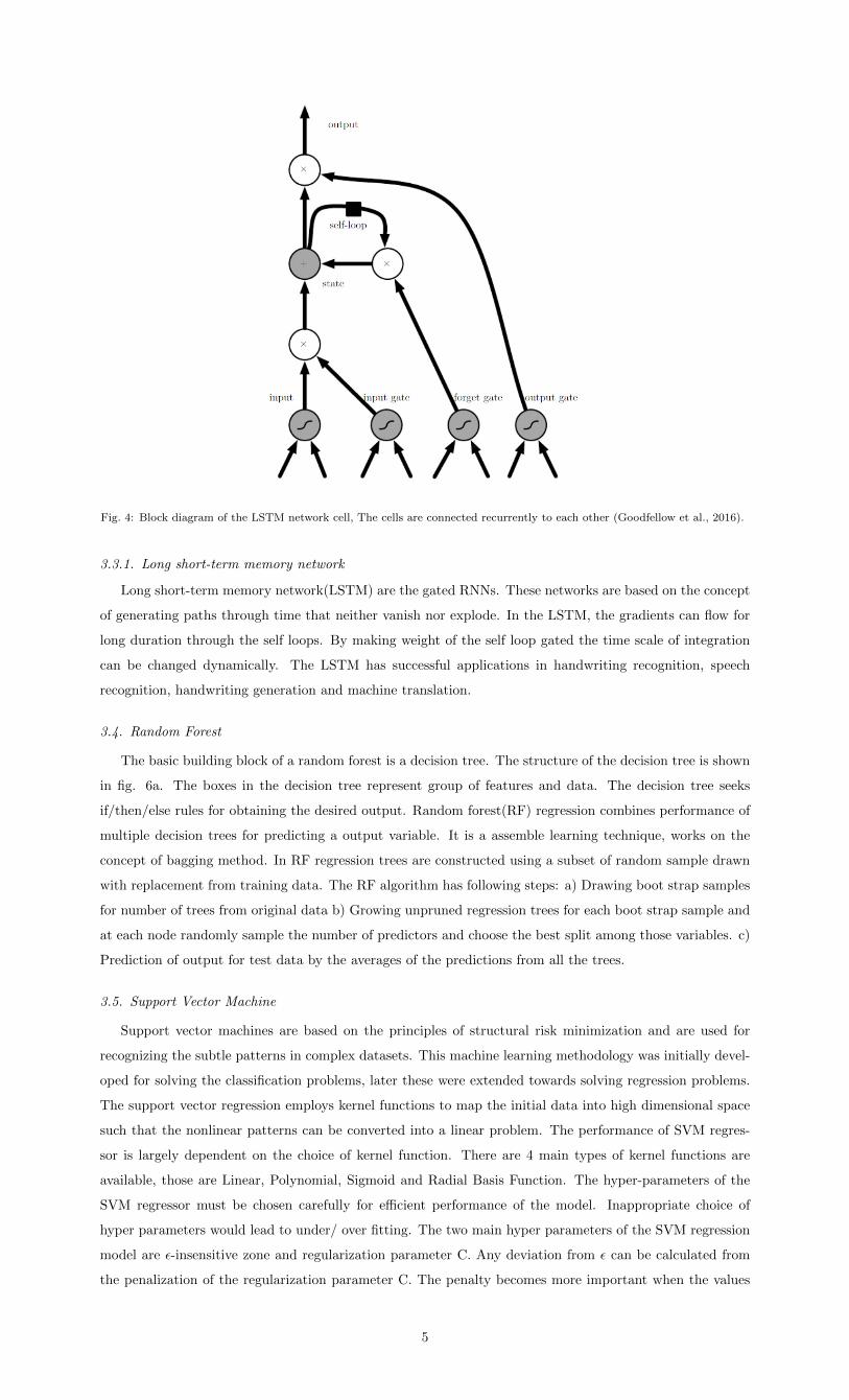
Fig. 4: Block diagram of the LSTM network cell, The cells are connected recurrently to each other (Goodfellow et al., 2016).
3.3.1. Long short-term memory network
Long short-term memory network(LSTM) are the gated RNNs. These networks are based on the concept
of generating paths through time that neither vanish nor explode. In the LSTM, the gradients can flow for
long duration through the self loops. By making weight of the self loop gated the time scale of integration
can be changed dynamically. The LSTM has successful applications in handwriting recognition, speech
recognition, handwriting generation and machine translation.
3.4. Random Forest
The basic building block of a random forest is a decision tree. The structure of the decision tree is shown
in fig. 6a. The boxes in the decision tree represent group of features and data. The decision tree seeks
if/then/else rules for obtaining the desired output. Random forest(RF) regression combines performance of
multiple decision trees for predicting a output variable. It is a assemble learning technique, works on the
concept of bagging method. In RF regression trees are constructed using a subset of random sample drawn
with replacement from training data. The RF algorithm has following steps: a) Drawing boot strap samples
for number of trees from original data b) Growing unpruned regression trees for each boot strap sample and
at each node randomly sample the number of predictors and choose the best split among those variables. c)
Prediction of output for test data by the averages of the predictions from all the trees.
3.5. Support Vector Machine
Support vector machines are based on the principles of structural risk minimization and are used for
recognizing the subtle patterns in complex datasets. This machine learning methodology was initially devel-
oped for solving the classification problems, later these were extended towards solving regression problems.
The support vector regression employs kernel functions to map the initial data into high dimensional space
such that the nonlinear patterns can be converted into a linear problem. The performance of SVM regres-
sor is largely dependent on the choice of kernel function. There are 4 main types of kernel functions are
available, those are Linear, Polynomial, Sigmoid and Radial Basis Function. The hyper-parameters of the
SVM regressor must be chosen carefully for efficient performance of the model. Inappropriate choice of
hyper parameters would lead to under/ over fitting. The two main hyper parameters of the SVM regression
model are ε-insensitive zone and regularization parameter C. Any deviation from ε can be calculated from
the penalization of the regularization parameter C. The penalty becomes more important when the values
5

Fig. 5: Architecture of CNN
Fig. 6: Architecture of of a random forest, a)a single decision tree b)a random forest
of C is higher and SVR fits the data. The penalty becomes negligible, when the value of C is small and SVR
gets flat. For higher value of ε SVR becomes flat and for smaller value of ε, SVR fits data.
4. Application of Machine learning in the marine environment
4.1. Wave forecasting
Waves are generated by complex interaction of wind with the ocean and the process by which ocean
waves are generated is not fully understood and is extremely uncertain and complex. The information of
wave heights at different locations is essential for operation related activities in the ocean. Most of the
works related to operation activities in the ocean are carried out with wave heights estimated over a period
of some hours or days. Traditionally deterministic models are used for prediction of height of waves and
wave periods (Sandhya et al., 2014). The ocean waves can both be forecasted and hindcasted using different
physics based approaches. Waves can be forecasted using meterological conditions and can be hindcasted
with different meterological charts. In wave forecasting, differential equations for wind-wave relationship and
wave energy are solved numerically. The methods using differential equations generally predict wave heights
for a period of 6-72 hours. The cost of numerical simulations using differential equations is very high and
the simulations are time consuming and the numerical predictions are always associated with uncertainties.
The uncertainties appears in the prediction results because of the approximations utilized in the model
development.
Because of the limitations in the traditional methods of wave height predictions and the rapid development
of ML methods, now researchers have started utilizing various ML algorithms (Mafi and Amirinia, 2017;
Etemad-Shahidi and Mahjoobi, 2009; Deka and Prahlada, 2012; Wang et al., 2018a; Law et al., 2020; Oliveira
et al., 2020; Deshmukh et al., 2016) such as neural networks (Deo et al., 2001; Deo and Naidu, 1998; Sahoo
and Bhaskaran, 2019), recurrent neural networks (Mandal and Prabaharan, 2006) and random forests for
prediction of wave heights. Deo et al. (2001) have used a simple 3 layered feed forward neural network to
predict the significant wave height and wave period. They considered the wind speed as input to the neural
network for March 1988 to July 1988 and further from December 1988 to May 1989. The location of the
data collection point was off Karwar in India. The ANN prediction of wave height is shown in fig. 7. Tsai
6

Fig. 7: Neural network prediction of wave heights and periods (Deo et al., 2001).
and Tsai (2009) have used ANN to predict the significant wave height, significant wave period, maximum
wave height and spectral peakedness parameter. The input parameters of the neural network are : average
of the highest one third pressure wave heights, corresponding pressure wave period, average pressure zero-
crossing period, maximum pressure wave height , average pressure wave height, root mean square pressure
wave height, average of one-tenth highest pressure wave height, successive pressure wave height correlation
and pressure spectral peakedness parameter. The detailed definitions of the above parameters are available
in (Tsai and Tsai, 2009). The ANN model was trained using data obtained from stations ranged from 11
to 41 m. The predicted results are compared with the results obtained from linear theory. The ANN model
predicted better results for water depths in between 20 to 41 meter in comparison to the linear theory. Rao
and Mandal (2005) used neural networks to estimate wave parameters from cyclone generated wind fields.
They considered 11 cyclones, which crossed the southern east coast of India in their studies. The inputs to
the neural network are difference between central and peripheral pressure, radius of maximum wind and the
speed of forward motion of cyclone. The outputs of the neural network are wave heights and periods. They
considered the feed forward neural network with back propagation algorithm in their modelling. The NN
model predictions are contrasted against other established wave hindcasting models and the observed very
good correlation between NN and physics based model results.
Oh and Suh (2018) used wavelet and neural network hybrid models for real-time forecasting of wave
heights. They developed the hybrid model by combining empirical orthogonal function analysis and wavelet
analysis with the neural network and used wave height data at different locations and meteorological data
in the surrounding are for training the ANN model. Their developed model was useful for prediction of
wave heights where past wave height and meteorological data are available. Doong et al. used ANN based
models to predict the the occurrence of coastal freak waves. An actual picture of a coastal freak wave is
shown in fig. 9. These waves are generated by interaction of waves with various coastal structures such as
rocks. They used seven parameters(significant wave height, peak period, wind speed, wave groupiness factor,
Benjamin Feir Index (BFI), kurtosis, and wind-wave direction misalignment) for training their model. They
used a single hidden layer neural network with back propagation algorithm. The field data used in their
study were collected from the Longdong Data Buoy(Central weather bureau of Taiwan). The buoy was at a
location of 1 km off the Longdong coast, where the water depth was 23m. Choi et al. (2020) used deep neural
networks to estimate significant wave height using raw ocean images8. A CNN based classification model was
constructed with four CNN structures. Their method of wave height prediction had two steps: a) the best
CNN model for ocean image processing was found among VGGNet, Inception.v3, ResNet and DenseNet. b)
The model performance was improved using transfer learning and structure modification. It was observed
that the VGGNet and ResNet based model with transfer learning and various feature extractors yielded
good performance in significant wave height modeling.
Traditionally strom surges are predicted using fluid dynamics methods(finite difference method) that
utilizes large number of equations and the simulations are time consuming. Rajasekaran et al. (2008) applied
support vector regression methodology to forecast typhoon surge. The typhoon surge must be accurately
predicted to avoid property loss. For the development of ML model they used the input data are pressure,
7

Fig. 8: Raw ocean images (Choi et al., 2020).
Fig. 9: An actual picture of a coastal freak wave (Doong et al., 2018).
wind velocity, wind direction and estimated astronomical tide and the out put is the storm surge level.
The ML model developed with support vector regression was verified using original data collected at the
Longdong station at Taiwan for the Aere typhoon. The location of the Longdong harbour is shown in fig.
10. Malekmohamadi et al. (2011) evaluated the efficacy of support vector machine, bayesian networks and
artificial neural networks in predicting the wave height. The data required for training the models were
collected at a buoy station at Lake Superior. They noticed ANN prediction of the wave height matched well
with the observational data and are better than prediction of the other ML models.
4.2. AUV operation and control
An AUV(autonomous underwater vehicle) is a self propelled unmanned vehicle, that can conduct various
activities in the deepest corners of Ocean or near the free surface (Tyagi and Sen, 2006). These don’t involve
any human supervision. Typical applications of AUV includes, sea floor mapping for construction of offshore
structures, characterization physical chemical and biological properties of ocean, Oceanographic applications
and many more. Since there is minimal human supervision for AUV operation, design of accurate control
system of AUV plays major role in the design of AUV. These vehicles have are robotic devices with own
propulsion system for navigation and have onboard computer for decision making (Sahoo et al., 2019).
Machine learning techniques has various application in the design of control system of the AUV. Zhang
et al. (2020) used neural networks for modelling an adaptive trajectory tracking control scheme for under
actuated autonomous underwater. The AUV was subjected to unknown asymmetrical actuator saturation
8

Fig. 10: Locations of Longdong harbour, Taiwan (Rajasekaran et al., 2008).
Fig. 11: Schematic of the DI-SMANNC for hybrid visual servoing of an underwater vehicle (Gao et al., 2017).
and unknown dynamics. The AUV kinematic controller was designed by using neural network compensa-
tion and adaptive estimation techniques. The neural network was used to approximate the complex AUV
hydrodynamics and differential of desired tracking velocities. The stability of the NN model was tested
against Lyapunov theory and backstepping technique. Zhang et al. (2018) proposed a novel bilateral adap-
tive control scheme for achieving position and force coordination performance of underwater manipulator
teleoperation system under model uncertainty and external disturbance. A new nonlinear model reference
adaptive impedance controller with bound-gain-forgetting (BGF) composite adaptive law is designed for the
master manipulator force tracking of the slave manipulator. They have used a radial basis function neural
network for local approximation of slave manipulator’s position tracking. The RBFNN based on Ge-Lee
(GL) matrix is adopted to directly approximate each element of the slave manipulator dynamic, and the
robust term with a proper update law is designed to suppress the error between the estimate model and the
real model, and the external disturbance. Gao et al. (2017) proposed a hybrid visual servo(HVS) controller
for underwater vehicles using a dynamic inversion based sliding mode adaptive neural network control. The
method was developed for tracking the HVS reference trajectory generated from a constant target pose. The
dynamic uncertainties were compensated using a single layer feed forward neural network, with an adaptive
sliding mode controller. The control system proposed was composed of a sliding model controller combined
with a neural network compensator is employed to construct a pseudo control signal required to track a
smooth reference trajectory, that is generated by a target pose through a reference model. A dynamic inver-
sion module was also incorporated in the control system to convert the pseudo control into actual thruster
control signals by using approximate dynamic model of underwater vehicles. The schematic of the proposed
control system architecture is shown in fig.11. Chu et al. (2016) proposed an observer based adaptive neural
network control approach for a class of remotely operated vehicles whose velocity and angular velocity state
9

in the body fixed frame are unmeasured. The thruster control signal was considered as the input to the
tracking control system. An adaptive state observer based on local recurrent neural network was proposed
to estimate the velocity and angular velocity state online. The adaptive learning method was also used to
estimate the scale factor of the thrust model.
4.3. Machine learning applied in ship research
4.3.1. Estimation of ship parameters
Ray et al. (1996) utilized neural networks to predict container capacity of a container ship. They used
database of previously built ships to predict the number of containers which can be accommodated on a vessel
and to design a container stowage plan. The input to the neural network are the length, breadth, depth,
deadweight and speed of the vessel and the output is the container capacity(number of containers). Margari
et al. (2018) used artificial neural networks to predict the resistance hullforms. The hull forms are sixteen
in number and those were mainly designed to be used as bulk carriers and tankers by the U.S. Maritime
Admisistration. The experimental data for the residual resistance coefficient were used to train and test a
series of neural networks. They considered a feed forward multilayered perception in their analysis. The
input vector to the neural network consists of length to breadth ratio, the breadth to draft ratio, the block
coefficient and the Froude number and the output is the residual resistance coefficient. Cepowski (2020)
predicted the added resistance of a ship in regular head waves. Experimental data collected from model test
measurements was used to train the neural network model. The predicted added resistance has applications
in the preliminary design stage. The function for the added mass coefficient was approximated as:
CAW = f(LBP,B, d, CB,Fn, λ/LBP ) (5)
where: LBP is the length between perpendiculars, B is the breadth, d is the draught,CB is the block
coefficient, Fn is the Froude number, λ is the wave length and f is the function for the prediction of ship added
resistance coefficient. Zhang and Zou (2013) used support vector machine for estimation of hydrodynamic
coefficients in the mathematical models of ship manoeuvring motion from captive model test results. The
towing test and pure sway test were also considered in the model testing. The comparison of the test data
and SVM predicted results suggest that, SVM is an effective method in predicting hydrodynamic coefficients
in captive model test. They also noticed that, the SVM model predictions are comparatively poor, for
polluted test data and uncertainties in the hydrodynamic models. The efficacy of SVM with polluted test
data can be enhanced by treating test data with de-noising approaches. Xu and Soares (2019) used a least
square support vector machine for estimation of parameters nonlinear manoeuvring model in shallow water.
4.3.2. Automatic Ship docking
Shuai et al. (2019) proposed an ANN based approach for automatic ship docking in presence of environ-
mental disturbances (12). The data required for ANN training was obtained by operating the ship by a skilled
captain using a joystick to control ship’s rudder and thrust. In the ANN based controller model the inputs
are the parameters selected from data analysis(those are state of vessel and environmental information) and
the output are the ship’s propeller speed and rudder angle. The vessel’s state are its heading and position,
speed of the vessel, the force of vessel in different degrees of freedom, and the environmental information
are force of wind in each degrees of freedom, the wind speed and wind direction.They used gradient descent
method to minimize the mean square error between the required output value and the actual output value
of the neural network. Based on sensitivity the optimal parameters for the ANN input are chosen as relative
distance between ship and dock and the heading angle. The output of the ANN is rudder angle and thruster
speed.
4.3.3. Ship manoeuvring simulation
Luo et al. (2014) used support vector regression for manoeuvring simulation of catamaran. The implicit
models are derived for the manoeuvring motion, instead of the traditional method of calculation hydrody-
namic coefficients. For development of the SVM regressor model data obtained from full scale trials were
10

Fig. 12: Schematic of the ANN based control strategy for automated ship docking (Shuai et al., 2019).
Fig. 13: Kinematic parameters in ship manoeuvring simulation, detailed definition of these parameters are available in Luo
et al. (2014)
used. The effects of wind and current induced disturbances were also considered in the model development.
The inputs to the SVM model were rudder angle, surge speed, yaw rate and sway speed respectively and
outputs are derivatives of the surge speed,sway speed and yaw rate respectively. They utilized Gauss function
kernel in the SVM to improve the performance of the approximation.
4.3.4. ship trajectory prediction
Tang et al. (2019) used Long Short-Term Memory(LSTM) network to model and predict the trajectories
of the vessels. The ground truth automatic identification data in the Tianjin port of China was used to
train and test the ML model. The inputs to the LSTM model are geographical location, speed, heading
and other status information and the output is the status of ship at any future moment. It was observed
that, the predicted trajectories are better than the traditional kalman filter model. The predicted trajectory
of the ship is shown in fig. 14. In the figure, the first 10 minute trajectory data was used to train the
LSTM model and the trajectory after 10th to 20th minute was predicted by the LSTM model. Volkova et al.
(2021) applied artificial neural networks(ANN) to predict trajectory of the ship. THE AIS data were used
for the ANN model development.This method of trajectory planning is mainly useful for river vessels and
river-sea vessels, when the vessel is near a hydraulic structure and there is problem in obtaining satellite
signals because of interference. The likelihood of collision can be decreased with application of ML based
trajectory prediction models.
4.3.5. Calculation of wind load on ship
Wind loads on ships, is an important parameter that need to calculated accurately, because that is
directly correlated with analysis of ship stability, maneuvering, station keeping and ship speed estimation.
Valcic and Prpic-Orsic (2016) developed a radial basis function neural network model by using elliptic Fourier
11

Fig. 14: Trajectory prediction of the ship (Tang et al., 2019).
Fig. 15: Box-plot of shaft power vs GPS speed (Parkes et al., 2018).
features of closed contours and wind load data collected from wind load data of three types of ships, those
are car carriers, container ships and offshore supply vessels. The trained neural network was employed for
the prediction of non-dimensional wind load coefficients.
4.3.6. Shaft power prediction of large merchant ships
Parkes et al. (2018) used neural networks to predict shaft power of large merchant ships. The data
required for training the neural network model was obtained from a data-set of 27 months of continuously
monitored data sampled in every 5 minutes from three vessels of same design(Sample data is shown in fig.15
reproduced from Parkes et al. (2018). The data consists of vessel movements recorded with varied geographic
locations and weather conditions. The variables used in training of the neural network model are GPS ship
speed, ship speed through water, true wind speed, apparent wind direction, draught, headings, trim and
wave height. The above mentioned parameters/features were used as input to the neural network model and
the output of the neural network is the shaft power. The shaft power is the product of shaft torque and
angular velocity. From accurate measurement of shaft power the engine efficiency can be calculated.
12

Fig. 16: ANN based model framework for fuel consumption prediction (Farag and Olcer, 2020).
4.3.7. Prediction of fuel consumption of ship main engine
Gkerekos et al. (2019) predicted the fuel consumption of main ship engine using different machine learning
algorithms, those are support vector machines, random forest regressors, tree regressors, ensemble methods
and artificial neural networks. Gkerekos et al. (2019) mainly compared the predictive capability of above
mentioned models in the prediction of the fuel consumption. Two different ship board data-sets were collected
using two different strategies of data collection, noon reports and automated data logging and monitoring,
were used for the model development. The ML models developed using different algorithms were found to be
accurately predict the fuel consumption under different weather condition, load condition, sailing distance,
drafts and speed. Farag and Olcer (2020) used ANN and multi-regression techniques to estimate the ship
power and fuel consumption. The data used for the ML model development was obtained from Farag (2017).
The data-set consists of data from two sea voyages collected at different loading conditions. Gkerekos and
Lazakis (2020) also used deep neural networks to develop a fuel consummation model and used that model in
the route optimisation process. Karagiannidis and Themelis (2021) feed forward neural networks to predict
the ship fuel consumption. The effect of data prepossessing on the model predictive accuracy was mainly
analyzed. Yuan et al. (2021) used LSTM to model the real time fuel consumption of vessels and utilized the
ML model to optimize the fuel consumption of the inland vessel using Reduced Space Searching Algorithm.
4.3.8. Ship collision avoidance
Gao and Shi (2020) used generative adversarial network(GAN) to generate appropriate anthropomorphic
collision avoidance decisions and bypass the process of ship collision risk assessment based on the quantifi-
cation of a series of functions. The LSTM cell was combined with GAN to improve capacity of memory
and the current availability of the overall system. The data required for the development of the ML model
was obtained from ship encounter azimuth map. The data-set has 12 types of ship encounter modes from
automatic identification system(AIS) big data (Yang et al., 2021). The proposed ML model can be applied
in intelligent collision avoidance, route planning and operational efficiency estimation.
13

4.4. Design and reliability analysis of breakwaters
Breakwaters are constructed in ports and harbors to prevent an anchorage from the erosion from the harsh
wave climate and long shore drift. The breakwaters the intensity of wave action in the ocean(Panduranga
et al., 2021; Kaligatla et al., 2021; Vijay et al., 2020).
Kim and Park (2005) used artificial neural networks to design and reliability analysis rubble mound
breakwater. The inputs to the neural networks are chosen by taking different combinations of the variables,
P , N , Sd, ζm, cosθ, h/Hs, SS, h/Ls and Ts. h/Hs is the water depth parameter, Ls is the period of
significant wave, h/Hs is the significant wave height, P is the permeability of the breakwater, N is the
number of wave attack and the other parameters have their usual meaning as used in breakwater reliability
analysis(Kim and Park, 2005). Based on different input combinations they used five neural networks to model
the stability of the breakwater and the predictions of the neural networks are compared against conventional
empirical model of Van Der Meer (1990). The stability model of Van Der Meer (1990) has the from:
Ns = 6.2P 0.18(Sd√Nw
)0.21√ζm
(6)
for ζm < ζc.
Kim et al. (2014) have used ANN to estimate the damage of breakwaters considering tidal level variations.
They employed the wave height prediction neural network into a Montecarlo simulation. The ANN was used
to predict the wave height in front of the breakwater. The inputs to the ANN are deep sea wave height and
the other was the tidal level in front of the breakwater and the significant wave height is the output of the
ANN.
4.5. Detection of damaged mooring lines
Chung et al. (2020) used ANN to detect the damaged mooring line in tension leg platform through
pattern analysis of floater responses. They used numerical simulation data(time series data of environment
and floater responses) of charm3D for training and testing of the neural network. The environmental data
are related to wave and wind, while the floater response data are related to the six degrees of freedom:
surge,sway, heave, roll, pitch and yaw. They considered a ANN with five hidden layers in their modeling.
The number of nodes in each layer as follows (16,100,300,500,300,100,9). 16 and 9 correspond to the first
and last layer and other numbers indicate the number of neuron in respective hidden layers. Their ANN
model was a classification network, whose job was to detect which mooring line is damaged by assigning an
explicit label to it. Aqdam et al. (2018) used radial basis function neural network to detect the fault in the
mooring line. The effects of uncertainties in the modeling (material, boundary, measurement uncertainties,
hydrodynamic effects) were considered in developing the ML models.
4.6. Machine learning applied in propeller research
Propellers are used in ships and submarines to create thrust to propel the vehicle (Prabhu et al., 2017;
Kumar et al., 2017; Nandy et al., 2018) . The blades are designed in such a manner so that their rotational
movement through the fluid generates a pressure difference between the two surfaces of blades. The pro-
pellers used in marine Engineering applications are mostly screw propellers with helical blades rotating on a
propeller shaft. Mahmoodi et al. (2019) used gene expression programming(GEP) to evaluate hydrodynamic
performance and cavitation volume of the marine propeller with various geometrical and physical conditions.
CFD data of propeller thrust, torque and cavitation volume at different rake angle, pitch ratio, skew an-
gle, advance velocity ratio and cavitation number are utilized in the development of the GEP model. The
mathematical expressions are developed for torque, thrust and cavitation volume in terms of the physical
and geometrical parameters. Shora et al. (2018) used ANNs to predict the hydrodynamic performance and
cavitation volume of propellers at different operating conditions. The data utilized in training and testing of
the ANN model was obtained from CFD simulations of the flow past the propeller with varied geometrical
and physical parameters. The input variables to the neural network are taken as rake angle, skew angle,
14

Fig. 17: Neural network used in modeling of the propeller induced erosion (Luo et al., 2014).
pitch ratio, advanced ratio and cavitation number and the output variables are propeller thrust, propeller
torque and cavitation volume. They generated 180 different data-sets by varying the input parameters. For
different output, they considered different configuration of ANN for minimum mean squared error. They
considered feed-forward and back-propagation ANNs in their simulations. Their ANN models very good
prediction accuracy(greater than 0.99). Kim et al. (2021) used convolutional neural networks to study the
risk of propeller cavitation erosion. The CNN model was trained using various ship model test results of
cavitation characteristics. Three types of CNN were used for the ML model development, those are VGG,
GoogleNet and ResNet. Ryan et al. (2013) used ANN to model propeller induced erosion alongside quay
walls in shallow water harbours and compared the predictive capability of the ANN by contrasting the results
with other regression based models. The structure of the ANN used in modeling of the propeller induced
erosion is shown in fig. 17. The ANN has five inputs, one output and six hidden layers. The input param-
eters to the neural network are Clarence distance from propeller tip to bed, propeller diameter, distance to
quay wall, rudder angle and densimetric Froude number and the output of the neural network is the depth
of maximum scour at a particular time instant. The data required for the ANN model was obtained from
deep rectangular GRP-lined plywood tank, using two open propellers.
4.7. Damage detection of offshore platforms
Offshore platforms are large structures installed in deep seas with facilities drilling of well to explore
natural gas and petroleum that lies in the seabed. These are damaged during their service life, because
of complex marine environments and human factors. In order to ensure the safety of marine operations,
the structural health monitoring such as, vibration based damage detection technique must be employed.
The vibration based damage detection method can identify the presence, location severity of the damages
of structures. Bao et al. (2021) used one-dimensional convolutional networks to detect the damage sensitive
features automatically from a offshore platform using raw strain response data. The CNN model was
validated using numerical simulations of jacket-type offshore platform for random and regular wave excitation
in different directions. Different damage locations and the noise effect were considered for finding the damage
localization and damage severity. The feature extraction capability of the CNN was enhanced using the data
pre-processing procedure based on convolution and deconvolution for noisy data. The CNN model developed
was tested for three different cases: e.g. offshore platform subject to a sinusoidal excitation, a white noise
extraction and a impulse excitation. Basically the model of Bao et al. (2021) is an extension of the work of
Abdeljaber et al. (2017), in which they had used CNN to detect the damage of a grandstand simulator at
Qatar University.
15

Fig. 18: Types of sandy beaches.(A) open sand beach.(B) supported sand beach.(C) bi-supported sand beach.(D) enclosed sand
beach Lopez et al. (2015).
4.8. Miscellaneous applications in the marine environment
4.8.1. Beach classification
Lopez et al. (2015) applied SVM and ANN to classify nine different types of beaches, those are mainly
micro-tidal sand and gravel beaches. The beach types are a) sand and gravel beaches, b) sand and gravel
separated beaches, c) gravel and sand separated beaches, d) Gravel and sand beaches, e) pure gravel beaches,
f) supported sand beaches, g) open sand beaches, h) bi-supported sand beaches, i) enclosed beaches. The ML
model results are compared with results of discriminant analysis. The 14 variables used in the classification
model development are: modality, D50, D10, D90, source, breaking wave height perpendicular to the beach,
frequency, direction associated with the wave height perpendicular to the beach, length profile, type profile,
slope of the berm, distance to the source and Posidonia depth. The above mentioned terms has their usual
definitions and is available in Lopez et al. (2015). The ML models developed with the above 14 variables,
were optimized with variation of neurons in the hidden layers and the SVM was modelled with different
kernels, those are linear, polynomial, radial basis function and sigmoid.
4.8.2. Condition monitoring of marine machinery system
Condition based maintenance is an advanced data-driven method of machine maintenance, in which
historical data collected by shipboard monitoring system is utilized by intelligence analysis tool to guide the
planned maintenance. This makes the machine maintenance work, more scientific, systematic, and planned.
Tan et al. (2020) used one class classification technology, that needs one class samples to train the model.
Six different classifiers were used in the modeling of the condition monitoring system, those are one class
support vector machine, support vector data description, Global k-nearest neighbors, Local outlier factor,
Isolation forest, Angle-based outlier detection. In the development of ML models, the data-set of marine gas
turbine propulsion system was used.
4.8.3. Performance assessment of shipping operations
Energy efficient operations can lead to reduced fuel consumption and reduction in environment pollution.
The improvements in the energy use efficiency can be achieved both by technical upgrades and through
16

Fig. 19: Schematic of the support vector machine classification. A non-linear mapping was used to map the observations into
a higher dimensional space Pagoropoulos et al. (2017).
Fig. 20: The block diagram of close loop optimal automated water blasting Le et al. (2021).
behavioural changes of the on board crew members. Pagoropoulos et al. (2017) used multi-class support
vector machines to identify the presence of energy efficient operations. The support vector machine utilized
a radial basis function kernel, that facilitates the adaptive modeling of the interface between the classes and
thus significantly improves classification performance as shown in fig.19. The data required for developing
the ML model was obtained through discussions with senior officers and technical superintends(mainly the
positive and negative patterns of energy efficient operations were identified). The main source of data utilized
in the model development was collected from noon reports (Poulsen and Johnson, 2016) and based on the
noon reports the energy consumption data were divided per consumer and covered the auxiliary machine
parts used for generation of electricity, boilers, main engine, pumps and incinerators.
4.8.4. Autonomous ship hull corrosion cleaning system
The ships can be smoothly operated with cleaning of the hulls in shipyards. Le et al. (2021) used
autonomous system based on reinforcement learning (Sutton and Barto, 2018) to remove the corrosion of a
ship by water blasting. The cleaning of ships by autonomous robotic systems ensure reduced consumption
of water, time and energy in contrast to the manual cleaning. Le et al. (2021) developed a water blasting
framework for a novel robot platform, which can navigate smoothly on a vertical plane and is designed with
the adhesion mechanism of a permanent magnet. In order to ensure shortest travel distance and time to save
resources used in the cleaning process, the complete way-point path planning is modeled as a classic travel
salesman problem. The level of corroded areas after water-blasting was assessed by using deep convolutional
neural networks. A detailed discussion of the operation strategy of the robot is available in Le et al. (2021).
The block diagram of the close loop optimal automated water blasting is shown in fig.20.
4.8.5. Wave energy forecasting
Wave energy is a promising source of renewable energy. Bento et al. (2021) employed artificial neural
networks to predict wave energy flux and other wave parameters. The The neural network model optimized
using moth-flame optimization and the proposed model was assessed using 13 different data-sets collected
from locations across the Atlantic, Pacific coast and Gulf of Mexico. Mousavi et al. (2021) used LSTM to
forecast power generation of a wave energy converter using artificial neural networks. The effective forecast
17

Fig. 21: A finite element model of 3-span suspension bridge with 2 floating pylons (Xu et al., 2020).
of wave energy will lead to reduced cost of investment in construction of the device and it is also essential
for operation and management of electric power. They have used both experimental and numerical data for
training and testing of the model. The experimental data was utilized from He (2020) and the numerical data
was obtained from numerical simulations using Flow-3D software. In their study, a ML model was developed
for a correlation between wave height and the generated electric power. Vieira et al. (2021) developed a novel
time efficient approach to calibrate VARANS-VOF models for simulation of wave interaction with porous
structures using Artificial Neural Networks. These methods are useful for reducing time consumption in
predicting the wave parameters using traditional fluid dynamics methods.
4.8.6. Prediction of wind and wave induced load effects on floating suspension bridges
Xu et al. (2020) used ANN and SVM to predict long-term extreme load effects of floating suspension
bridges. They used ML models as surrogate models, in conjunction with the Monte-carlo based methods,
for the faster prediction of the loads. For their case study a 3-span suspension bridge with 2 floating pylons
under combined wind and wave actions was used as shown in fig.21. In the new Monte-Carlo framework, the
implicit limit-state function was replaced by the surrogate models based on ANN and SVM. It was noticed
that, the ML based Monte-Carlo method require less computational effort and predicted more accurate
results.
4.8.7. Tidal current prediction
The traditional method of tidal current prediction employs computer applications with classical harmonic
analysis. Those are computationally expensive for real time predictions. Sarkar et al. (2018) used Bayesian
machine learning (Gaussian processes) for the prediction of tidal currents. With use of ML based techniques
the uncertainties and complexity of the problem were enabled to represent in the modeling basis. The
data used in the development of ML algorithm were collected from National Oceanic and Atmospheric
Administration (NOAA). The location of tidal current observation sites are Southampton Shoal Channel,
Old Port Tampa, Sunshine Sky Bridge and Martinez-AMORCO Pier. The data obtained from these sites
were used for long-term predictions. The Gaussian process with periodic kernel function was found to be
suitable for the modeling problem concerned, because of its harmonic nature. Immas et al. (2021) utilized
deep learning models to develop tools for in situ prediction of ocean currents, those are, a Long Short-Term
Memory (LSTM) Recurrent Neural Network and a Transformer. The data utilized for model development
were also obtained from NOAA. In addition to speed, they also predicted the direction of ocean currents.
It was noticed that the predictions of Ocean currents are more accurate in contrast to the predictions of
harmonic methods(Immas et al., 2021). Sumangala and Warrior (2020) used ANN to model the currents of
Bay of Bengal. They mainly improved the velocity predictions using ANN model.
4.9. Application of ML in CFD
The field of Naval Architecture, Ocean and Marine Engineering often employs CFD as a tool for modeling
and prediction of flow past ships and underwater vehicles (Panda and Warrior, 2021c; Mitra et al., 2019,
2020), visualization of flow past propellers (Prabhu et al., 2017), analysis of wave induced load on offshore
structures, simulations of waves and currents and simulations of wave energy converters (Mohapatra et al.,
18

Fig. 22: The SDF representation of base airfoil (Hui et al., 2020).
2021a,b; Mohapatra and Sahoo, 2020) . The commercial software used in CFD analysis are ANSYS FLUENT
(Fluent, 2011), STAR-CCM+ (CD-adapco, 2017) and SHIPFLOW (Larsson et al., 1989). CFD is cheaper in
comparison to experimental methods and can be applied for flow prediction in larger and complex domains,
like modeling flow past larger ships and predicting complex flow past propellers. The basic building block
of such CFD tools are turbulence models. In literature, ML techniques are either applied for faster flow
prediction using surrogate models or developing turbulence closure models using large data-sets of direct
numerical simulations(DNS) or experiments.
In this section, we will provide a detailed overview of application of ML algorithms in CFD and turbulence
modeling. The Naval Architects and CFD engineers working with different research problems may employ
such advanced techniques for modeling and prediction of the complex oceanic flow fields.
4.9.1. Fluid flow field prediction using reduced order models
Sekar et al. (2019) used deep neural networks for flow prediction over airfoils. They used a deep convo-
lutional neural network for extraction of features from the different shapes of the airfoil and utilized those
shape related features along with Reynolds number and angle of attack as inputs to the DNN model. The
outputs to the DNN are pressure and velocity components across the airfoil. The data required for training
the DNN model is obtained from CFD simulations. They predicted the flow field at much faster speed (150
times) in comparison to the traditional CFD methods and the results are as accurate as the traditional CFD
predictions. Hui et al. (2020) utilized CNN to predict pressure distribution around airfoils. The data-set
library was formed using numerical simulation data from deformed airfoils. The airfoil was parametrized
using the signed distance function(SDF). Renganathan et al. (2020) utilized DNN fro non-intrusive model
order reduction of the parametric inviscid transonic flow past an airfoil. They preserved the accuracy of
flow prediction at a significant lower computational cost. Kong et al. (2021a) used CNN to predict the
velocity field for flow in in a scramjet isolator. The data required for training model was obtained from
numerical simulations of flow at different Mach numbers and back pressures. The CNN has multiple recon-
struction and feature extraction modules. A mapping relationship was established between the wall pressure
on isolator and the velocity field on the isolator. Kong et al. (2021b) used DL approach for super-resolution
flow field reconstruction of a scramjet isolator. In contrast to the work of Kong et al. (2021a), Kong et al.
(2021b) used experimental data-sets for the development of the DL model. They used both single path and
multi-path network models based on CNNs for flow field reconstruction. It was noticed that the multi-path
CNNs has better predictive accuracy in comparison to the single path CNNs. Lee and You (2021) used
CNN for predicting unsteady volume wake three-dimensional flow fields. The ML model was trained with
past information of flow velocity and pressure. They also performed different analysis to find structural
19

Fig. 23: Sample input and output data for the point-net (Kashefi et al., 2021).
similarities among feature maps to reduce the number of feature maps containing redundant flow structures.
Such reduction process can decrease the size of neural network without affecting the prediction performance.
Hasegawa et al. (2020) developed a reduced order model(ROM) for unsteady flow prediction by combining
CNN and LSTM, which are trained in a sequential manner. The CNN model was trained using DNS data
obtained from numerical simulations with 80 bluff bodies and tested on 20 bluff bodies. They also tested
the ML-ROM model for unseen bluff bodies, and the predicted results were quite satisfactory, this shows
the universality of ML-ROM based models. Nakamura et al. (2021) modeled three dimensional complex flow
using ROM. The ROM consists of a CNN and a LSTM. The function CNN was to map high dimensional flow
fields into a low-dimensional latent space and the LSTM was used to predict temporal evolution of latent
vectors.The data required for training the ROM was obtained from DNS. Leer and Kempf (2021) utilized
MLP in conjuction with radial-logarithmic filter mask (RLF) for developing a universally applicable ML
concept fast flow field estimation for various geometry types. The function of RLF is to provide information
about the geometry in a compressed form for the MLP. They applied new concept for both internal and
external flows such as airfoils and car shapes. The ML model was developed with data generated from CFD
simulations for different geometries and the was tested for different unknown geometries.
Sun et al. (2020) proposed a physics constrained deep learning (DL) approach for surrogate modeling of
fluid flows. The surrogate model was developed without relying on CFD simulation data. They proposed a
structured DNN to enforce the initial and boundary conditions and the Navier-Stokes (NS) equation were
incorporated into the loss of the DNN in the training. Kashefi et al. (2021) proposed a novel deep learning
(DL) approach (Point net architecture) for flow prediction in irregular geometries when the flow field is either
a function of the size and shape of the bluff body or the shape of the domain. The grid vertices (spatial
positions) of the mesh in the CFD domain were taken as the input to the DL model and corresponding
flow parameters at those points were considered as output. The point net architecture learns the non-linear
relationship between the inputs and outputs. The Point net model was trained for in-compressible laminar
steady flow past a cylinder and for testing its generalizability, it was used for prediction of flow around
multiple objects and airfoils. The ML model predictions are found to be satisfactory and also accurate.
4.9.2. Turbulence modeling with ML
Turbulent flows are a classification of fluid flows that are characterised by the manifestation of spatio-
temporal chaos, hyper-sensitivity to perturbations, increased rates of diffusion, heat and mass transfer, etc.
As has been observed turbulence is the norm and not the exception in nature (Moin and Kim, 1997). In
engineering context the ability to predict the evolution of turbulence is of critical importance (Pope, 2000).
Because of the chaotic nature exact numerical prediction of turbulent flows is impracticable. Most engineering
CFD studies rely on turbulence models to account for turbulence. The accuracy of CFD simulations are
largely dependent on choice of turbulence models.
The simplest class of turbulence models are the mixing length based models, also referred to as one
equation models (Speziale, 1991). While these are simple and computationally inexpensive they require
extensive input parameters for each case. Many of these parameters cannot be determined without reliable
CFD simulations leading to a paradoxical situation. Because of this one equation models are not regularly
used in engineering applications. The second category of turbulence models is the eddy viscosity based models
20
that includes popular models like the k− ε, k−ω models. These use the concept of an eddy viscosity to form
a constitutive equation between the Reynolds stresses and the instantaneous mean gradients. Eddy viscosity
based models are universal, robust and computationally inexpensive. But they have significant limitations in
flows separation and re-attachment (Speziale et al., 1990; Mishra et al., 2019), flows around inhomogeneities
like walls (Pope, 2000), flows with moderate to high degrees of anisotropy (Pope, 2000; Mishra and Girimaji,
2019), etc. The final category of turbulence models are Reynolds Stress Models, that utilize the Reynolds
Stress Transport Equations to formulate individual transport equations for the components of the Reynolds
stress tensor. These include the Launder-Reece-Rodi (LRR) model (Launder et al., 1975), the Speziale-
Sarkar-Gatski (SSG) model (Speziale et al., 1991; Sarkar and Speziale, 1990), the Mishra-Girimaji model
(Mishra and Girimaji, 2013, 2017), etc. Reynolds stress models offer higher accuracy and robustness at a
higher computational cost. However Reynolds stress models have limitations as well especially in flows with
high influence of rotational effects (Mishra and Girimaji, 2010), significant streamline curvature (Mishra
and Girimaji, 2014), etc. We observe that while there are many different turbulence models, they all have
significant limitations that affect their accuracy, their applicability and their robustness. All the above
mentioned models are developed by calibrating the model coefficients with respect to experimental or direct
numerical simulation(DNS) data. With increase in computational facilities and data storage capacity and
advancements in the ML techniques, current emphasis of turbulence researchers have been shifted towards
development of turbulence models by using different ML algorithms (Jimenez, 2018) such as random forest,
gradient boosting trees and deep neural networks. In this section, a detailed discussion turbulence models
developed with ML approaches will be provided.
Duraisamy et al. (2015) proposed new methods in turbulence and transition modeling using neural
networks and Gaussian processes. They developed improved functional forms using ML and applied those
functional forms to predict the flow field. Singh et al. (2017) used neural networks for developing model
augmentations for the Spalart-Allmaras model. The model forms are constructed and incorporated into the
CFD solver. Ling et al. (2016) used deep neural networks to develop a model for Reynolds stress anisotropy
tensor by using high fidelity DNS data. They have proposed a new neural network (Tensor Basis Neural
Network) that can accommodate the invariant properties (Galilean Invariance) into the modeling basis.
The neural network structure was optimized using Bayesian optimizationSnoek et al. (2012). A significant
improvement in flow predictions were noticed when the ML model predictions are compared against the
baseline RANS models. A data-driven Physics Informed Machine Learning(PIML) approach was proposed
by Wang et al. (2017), in which the discrepancies in the RANS modeled Reynolds stresses were reconstructed.
They used Random forests for modeling of the discrepancies with DNS data and the model developed was
used to predict flow field for other flow cases, which were not used for model development. Wu et al. (2018)
proposed a systematic approach for choosing the input feature variables used in turbulence modeling. They
considered strain rate tensor, rotation rate tensor, pressure gradient, TKE gradient, Wall distance based
Reynolds number, turbulence intensity and ratio of turbulent time-scale to mean strain time-scale as the
input features to model the discrepancy between RANS modeled and true Reynolds stresses. They used
gradient of the flow features in place of the actual value to ensure Galilean invariance (Pope, 2000). Finally
the predictive capability of the ML model was tested against square duct and periodic hill flows. Kaandorp
and Dwight (2020) proposed Tensor Basis Random Forest(TBRF), a novel machine learning algorithm to
predict the Reynolds stress anisotropy tensor(RSAT). The use of tensor basis ensures the Galilean invariance
in the prediction of the RSAT. The TBRF was trained with various flow cases of DNS/LES data and was
tested for unseen flows. The predicted values of the RSAT was finally employed in a RANS solver for flow
prediction in unseen flows. Zhu et al. (2021) developed surrogate turbulence model for prediction of flow
past airfoils at high Reynolds numbers. Rather than using DNS or LES data, they utilized results from
numerical simulations of Spallart-Allmaras (SA) model for training the DNN. The model was trained with
six different six different free stream conditions for NACA0012 airfoil.
Panda and Warrior (2021b) have proposed a data-driven model for the pressure strain correlation of
21

turbulence(Panda and Warrior, 2018; Panda et al., 2020) using Reynolds stress anisotropy, dissipation, tur-
bulence kinetic energy and the strain rate as the input to the DNN . They used DNS data of flow in channels
at different friction Reynolds numbers for the development of the DNN based model and the model was
tested for flows in different Reynolds numbers and also for a fully unknown test case of Couette flow in chan-
nels. The model predictions was also contrasted against other established pressure strain correlation models.
Panda and Warrior (2021a) compared the predictive capability of random forest, gradient boosted tree and
DNN in Reynolds stress transport modeling. They mainly considered the modeling of the pressure strain
correlation of turbulence. Using Bayesian optimization they recommended the optimal hyper-parameters of
the DNN.
Wang et al. (2018b) proposed ML based subgrid-scale models(SGS) using DNN and RF for LES. They
considered 30 flow variables as inputs to the ML model and analysed the feature importance of input variables
and found that the filtered velocity and second derivative of the input velocity has larger influence on the
output variable. The newly proposed ANN based SGS model has a correlation coefficient of 0.7. The proposed
ANN based SGS model was found to be accurate than the Smagorinsky model and the dynamic Smagorinsky
model for flow predictions in isotropic turbulence. Yuan et al. (2020) used a deconvolutional artificial neural
network(DANN) for modeling SGS. The input features for the DANN are the filtered velocities at different
spatial points. It was observed that the DANN model predicted the SGS stress more accurately than the
approximate deconvolution method and the velocity gradient model with a corrrelation coefficient of 0.99.
Xie et al. (2020) developed ANN based algebraic models for the SGS in LES of turbulence at the Taylor
Reynolds number ranging from 180 to 250. They had constructed the coefficients of the non-linear algebraic
model using the ANN. It was shown that the ANN based non-linear algebraic model predicted the SGS
stress more accurately in a priori tests.
5. Challenges and Priority Research Directions
Machine learning applications are having significant successes and impact across different problems in
marine engineering, ocean engineering and naval architecture. Nonetheless we need to ensure a higher degree
of trust in ML models, enable adequate verification and validation (V&V) of data driven models, and utilize
the strengths of data driven algorithms together with the decades of purely physics based understanding
that has been developed in these fields (Hu et al., 2020).
An important step is to include physics and domain knowledge in machine learning models (Baker
et al., 2019). This can be done at various levels for example the choice of the model algorithm and its
hyperparameters, the features that are inputted to the algorithm, or directly appending physics constraints
in the loss functions and optimization. As an illustration we can enforce mass and momentum conservation
as constraints by appending additional losses that penalize the violation of these constraints in the loss
functions of the turbulence models generated by deep neural networks. This would ensure more physical
data driven models. This would also reduce the space of functions that the optimizer has to query over and
lead to better models that require less training data.
Another important step is generating measures of interpretability and explainability from ML models
(Zaman, 2020). As an illustration in physics based models that are commonplace in marine and ocean
engineering every term and each expression has physical meaning and represents different physics based
interactions and processes. Machine learning models do not allow such understanding and rationalization.
This lack of transparency leads to an understandable lack of trust in ML models from scientists and engi-
neers working in marine and ocean applications. This also obviates any model validation. Verification and
validation are essential steps to be executed before the deployment of any physics based models in marine
and ocean engineering and should be so for data driven models as well. Model verification for ML models
can be and is carried out using test datasets to estimate generalization error. For model validation we need
to be able to unearth the model’s reasoning for its predictions. Due to the black box nature of algorithms
like deep neural networks, this is not possible yet. Hence there is a critical need to interpret and explain the
22

reasoning of trained ML models before they can start to replace traditional physics and empiricism based
models.
A final need is to ensure robustness in the performance of ML models (Hegde, 2020). Traditional models
in marine and ocean applications have been based on physics. Physical laws such as symmetries, conservation
of mass, momentum and species, etc are universal and extend to all ranges of parameter space. But machine
learning models are restricted to the range where training data was utilized for their optimization. In regions
of feature space far from the training data ML models make extremely poor predictions. For their general
application there is a need to guarantee robustness in model performance.
6. Concluding remarks
In this article, we have provided a detailed review of application of machine learning algorithms in
ocean engineering, naval architecture and marine engineering applications. The different machine learning
algorithms are discussed in detail. The ML applications in the marine environment were classified into
several categories such as wave forecasting, AUV operation and control, ship research, design and reliability
analysis of breakwaters, applications in propeller research etc. The features used in modeling different marine
processes and parameters were discussed in detail. The source of data utilized in model development are
presented. The features used as inputs to the ML models are discussed in detail. Different algorithms used
in optimization of the ML models were also discussed. A detailed overview of application of ML in CFD and
turbulence modeling were also presented. Based on this comprehensive review and analysis we point out
future directions of research that may be fruitful for the application of ML to ocean and marine engineering
as well as problems in naval architecture. This review article will provide an avenue for marine engineers
and naval architects to learn the basics of ML models and its applications in the ocean engineering, naval
architecture and marine engineering applications.
23

References
Abdeljaber, O., Avci, O., Kiranyaz, S., Gabbouj, M., Inman, D.J., 2017. Real-time vibration-based structural
damage detection using one-dimensional convolutional neural networks. Journal of Sound and Vibration
388, 154–170.
Aqdam, H.R., Ettefagh, M.M., Hassannejad, R., 2018. Health monitoring of mooring lines in floating
structures using artificial neural networks. Ocean Engineering 164, 284–297.
Baker, N., Alexander, F., Bremer, T., Hagberg, A., Kevrekidis, Y., Najm, H., Parashar, M., Patra, A.,
Sethian, J., Wild, S., et al., 2019. Workshop report on basic research needs for scientific machine learning:
Core technologies for artificial intelligence. Technical Report. USDOE Office of Science (SC), Washington,
DC (United States).
Bao, X., Fan, T., Shi, C., Yang, G., 2021. One-dimensional convolutional neural network for damage
detection of jacket-type offshore platforms. Ocean Engineering 219, 108293.
Bento, P., Pombo, J., Mendes, R., Calado, M., Mariano, S., 2021. Ocean wave energy forecasting using
optimised deep learning neural networks. Ocean Engineering 219, 108372.
CD-adapco, S., 2017. Star ccm+ user guide version 12.04. CD-Adapco: New York, NY, USA .
Cepowski, T., 2020. The prediction of ship added resistance at the preliminary design stage by the use of
an artificial neural network. Ocean Engineering 195, 106657.
Cherkassky, V., Mulier, F.M., 2007. Learning from data: concepts, theory, and methods. John Wiley &
Sons.
Choi, H., Park, M., Son, G., Jeong, J., Park, J., Mo, K., Kang, P., 2020. Real-time significant wave height
estimation from raw ocean images based on 2d and 3d deep neural networks. Ocean Engineering 201,
107129.
Chu, Z., Zhu, D., Jan, G.E., 2016. Observer-based adaptive neural network control for a class of remotely
operated vehicles. Ocean Engineering 127, 82–89.
Chung, M., Kim, S., Lee, K., et al., 2020. Detection of damaged mooring line based on deep neural networks.
Ocean Engineering 209, 107522.
Creswell, A., White, T., Dumoulin, V., Arulkumaran, K., Sengupta, B., Bharath, A.A., 2018. Generative
adversarial networks: An overview. IEEE Signal Processing Magazine 35, 53–65.
Deka, P.C., Prahlada, R., 2012. Discrete wavelet neural network approach in significant wave height fore-
casting for multistep lead time. Ocean Engineering 43, 32–42.
Deo, M., Naidu, C.S., 1998. Real time wave forecasting using neural networks. Ocean engineering 26,
191–203.
Deo, M.C., Jha, A., Chaphekar, A., Ravikant, K., 2001. Neural networks for wave forecasting. Ocean
engineering 28, 889–898.
Deshmukh, A.N., Deo, M., Bhaskaran, P.K., Nair, T.B., Sandhya, K., 2016. Neural-network-based data
assimilation to improve numerical ocean wave forecast. IEEE Journal of Oceanic Engineering 41, 944–953.
Doong, D.J., Peng, J.P., Chen, Y.C., 2018. Development of a warning model for coastal freak wave occur-
rences using an artificial neural network. Ocean Engineering 169, 270–280.
Duraisamy, K., Zhang, Z.J., Singh, A.P., 2015. New approaches in turbulence and transition modeling using
data-driven techniques, in: 53rd AIAA Aerospace Sciences Meeting, p. 1284.
24

Etemad-Shahidi, A., Mahjoobi, J., 2009. Comparison between m5 model tree and neural networks for
prediction of significant wave height in lake superior. Ocean Engineering 36, 1175–1181.
Farag, Y.B., Olcer, A.I., 2020. The development of a ship performance model in varying operating conditions
based on ann and regression techniques. Ocean Engineering 198, 106972.
Farag, Y.B.A., 2017. A decision support system for ship’s energy efficient operation: based on artificial
neural network method. Thesis .
Fluent, A., 2011. Fluent 14.0 user’s guide. ANSYS FLUENT Inc .
Gao, J., An, X., Proctor, A., Bradley, C., 2017. Sliding mode adaptive neural network control for hybrid
visual servoing of underwater vehicles. Ocean Engineering 142, 666–675.
Gao, M., Shi, G.Y., 2020. Ship collision avoidance anthropomorphic decision-making for structured learning
based on ais with seq-cgan. Ocean Engineering 217, 107922.
Gkerekos, C., Lazakis, I., 2020. A novel, data-driven heuristic framework for vessel weather routing. Ocean
Engineering 197, 106887.
Gkerekos, C., Lazakis, I., Theotokatos, G., 2019. Machine learning models for predicting ship main engine
fuel oil consumption: A comparative study. Ocean Engineering 188, 106282.
Goodfellow, I., Bengio, Y., Courville, A., 2016. Deep learning. MIT press.
Hartigan, J.A., Wong, M.A., 1979. Algorithm as 136: A k-means clustering algorithm. Journal of the royal
statistical society. series c (applied statistics) 28, 100–108.
Hasegawa, K., Fukami, K., Murata, T., Fukagata, K., 2020. Machine-learning-based reduced-order modeling
for unsteady flows around bluff bodies of various shapes. Theoretical and Computational Fluid Dynamics
34, 367–383.
He, J., 2020. Coherence and cross-spectral density matrix analysis of random wind and wave in deep water.
Ocean Engineering 197, 106930.
Hegde, A.S., 2020. Quantifying the agreement between computational models and experimental data under
uncertainty. University of California, Berkeley.
Hu, X., Hu, H., Verma, S., Zhang, Z.L., 2020. Physics-guided deep neural networks for power flow analysis.
IEEE Transactions on Power Systems 36, 2082–2092.
Hui, X., Bai, J., Wang, H., Zhang, Y., 2020. Fast pressure distribution prediction of airfoils using deep
learning. Aerospace Science and Technology 105, 105949.
Immas, A., Do, N., Alam, M.R., 2021. Real-time in situ prediction of ocean currents. Ocean Engineering
228, 108922.
Jimenez, J., 2018. Machine-aided turbulence theory. Journal of Fluid Mechanics 854.
Kaandorp, M.L., Dwight, R.P., 2020. Data-driven modelling of the reynolds stress tensor using random
forests with invariance. Computers & Fluids 202, 104497.
Kaligatla, R., Sharma, M., Sahoo, T., 2021. Wave interaction with a pair of submerged floating tunnels
in the presence of an array of submerged porous breakwaters. Journal of Offshore Mechanics and Arctic
Engineering 143, 021402.
Karagiannidis, P., Themelis, N., 2021. Data-driven modelling of ship propulsion and the effect of data
pre-processing on the prediction of ship fuel consumption and speed loss. Ocean Engineering 222, 108616.
25

Kashefi, A., Rempe, D., Guibas, L.J., 2021. A point-cloud deep learning framework for prediction of fluid
flow fields on irregular geometries. Physics of Fluids 33, 027104.
Kim, D.H., Kim, Y.J., Hur, D.S., 2014. Artificial neural network based breakwater damage estimation
considering tidal level variation. Ocean engineering 87, 185–190.
Kim, D.H., Park, W.S., 2005. Neural network for design and reliability analysis of rubble mound breakwaters.
Ocean engineering 32, 1332–1349.
Kim, J.H., Lee, H., Hur, J.W., 2021. A study on the risk of propeller cavitation erosion using convolutional
neural network. Journal of the Society of Naval Architects of Korea 58, 129–136.
Kong, C., Chang, J., Li, Y., Wang, Z., 2021a. A deep learning approach for the velocity field prediction in
a scramjet isolator. Physics of Fluids 33, 026103.
Kong, C., Chang, J., Wang, Z., Li, Y., Bao, W., 2021b. Data-driven super-resolution reconstruction of
supersonic flow field by convolutional neural networks. AIP Advances 11, 065321.
Kumar, S., Nagarajan, V., Sha, O., 2017. Measurement of flow characteristics in propeller slipstream of a
twin propeller twin rudder model ship. International Shipbuilding Progress 63, 1–40.
Larsson, L., Broberg, L., Zhang, D., 1989. Shipflow–a cfd system for ship design, in: International Symposium
on Practical Design of Ships and Mobile Units (PRADS), 4th, pp. 53–65.
Launder, B., Reece, G.J., Rodi, W., 1975. Progress in the development of a reynolds-stress turbulence
closure. Journal of fluid mechanics 68, 537–566.
Law, Y., Santo, H., Lim, K., Chan, E., 2020. Deterministic wave prediction for unidirectional sea-states in
real-time using artificial neural network. Ocean Engineering 195, 106722.
Le, A.V., Kyaw, P.T., Veerajagadheswar, P., Muthugala, M.V.J., Elara, M.R., Kumar, M., Nhan, N.H.K.,
2021. Reinforcement learning-based optimal complete water-blasting for autonomous ship hull corrosion
cleaning system. Ocean Engineering 220, 108477.
Lee, S., You, D., 2021. Analysis of a convolutional neural network for predicting unsteady volume wake flow
fields. Physics of Fluids 33, 035152.
Leer, M., Kempf, A., 2021. Fast flow field estimation for various applications with a universally applicable
machine learning concept. Flow, Turbulence and Combustion 107, 175–200.
Ling, J., Kurzawski, A., Templeton, J., 2016. Reynolds averaged turbulence modelling using deep neural
networks with embedded invariance. Journal of Fluid Mechanics 807, 155–166.
Lopez, I., Aragones, L., Villacampa, Y., Compan, P., Satorre, R., 2015. Morphological classification of
microtidal sand and gravel beaches. Ocean engineering 109, 309–319.
Luo, W., Moreira, L., Soares, C.G., 2014. Manoeuvring simulation of catamaran by using implicit models
based on support vector machines. Ocean Engineering 82, 150–159.
Mafi, S., Amirinia, G., 2017. Forecasting hurricane wave height in gulf of mexico using soft computing
methods. Ocean Engineering 146, 352–362.
Mahmoodi, K., Ghassemi, H., Nowruzi, H., Shora, M.M., 2019. Prediction of the hydrodynamic performance
and cavitation volume of the marine propeller using gene expression programming. Ships and Offshore
Structures 14, 723–736.
Malekmohamadi, I., Bazargan-Lari, M.R., Kerachian, R., Nikoo, M.R., Fallahnia, M., 2011. Evaluating the
efficacy of svms, bns, anns and anfis in wave height prediction. Ocean Engineering 38, 487–497.
26

Mandal, S., Prabaharan, N., 2006. Ocean wave forecasting using recurrent neural networks. Ocean engineer-
ing 33, 1401–1410.
Margari, V., Kanellopoulou, A., Zaraphonitis, G., 2018. On the use of artificial neural networks for the calm
water resistance prediction of marad systematic series’ hullforms. Ocean Engineering 165, 528–537.
Mishra, A.A., Duraisamy, K., Iaccarino, G., 2019. Estimating uncertainty in homogeneous turbulence evo-
lution due to coarse-graining. Physics of Fluids 31, 025106.
Mishra, A.A., Girimaji, S., 2019. Linear analysis of non-local physics in homogeneous turbulent flows.
Physics of Fluids 31, 035102.
Mishra, A.A., Girimaji, S.S., 2010. Pressure–strain correlation modeling: towards achieving consistency with
rapid distortion theory. Flow, turbulence and combustion 85, 593–619.
Mishra, A.A., Girimaji, S.S., 2013. Intercomponent energy transfer in incompressible homogeneous tur-
bulence: multi-point physics and amenability to one-point closures. Journal of Fluid Mechanics 731,
639–681.
Mishra, A.A., Girimaji, S.S., 2014. On the realizability of pressure–strain closures. Journal of Fluid Mechanics
755, 535–560.
Mishra, A.A., Girimaji, S.S., 2017. Toward approximating non-local dynamics in single-point pressure–strain
correlation closures. Journal of Fluid Mechanics 811, 168–188.
Mitra, A., Panda, J., Warrior, H., 2019. The effects of free stream turbulence on the hydrodynamic charac-
teristics of an auv hull form. Ocean Engineering 174, 148–158.
Mitra, A., Panda, J.P., Warrior, H.V., 2020. Experimental and numerical investigation of the hydrody-
namic characteristics of autonomous underwater vehicles over sea-beds with complex topography. Ocean
Engineering 198, 106978.
Mohapatra, P., Sahoo, T., 2020. Hydrodynamic performance analysis of a shore fixed oscillating water
column wave energy converter in the presence of bottom variations. Proceedings of the Institution of
Mechanical Engineers, Part M: Journal of Engineering for the Maritime Environment 234, 37–47.
Mohapatra, P., Vijay, K., Bhattacharyya, A., Sahoo, T., 2021a. Performance of a shore fixed oscillating
water column device for different bottom slopes and front wall drafts: A study based on computational
fluid dynamics and biem. Journal of Offshore Mechanics and Arctic Engineering 143, 032002.
Mohapatra, P., Vijay, K., Bhattacharyya, A., Sahoo, T., 2021b. Performance of a shore fixed oscillating
water column device for different bottom slopes and front wall drafts: A study based on computational
fluid dynamics and biem. Journal of Offshore Mechanics and Arctic Engineering 143, 032002.
Moin, P., Kim, J., 1997. Tackling turbulence with supercomputers. Scientific American 276, 62–68.
Mousavi, S.M., Ghasemi, M., Manshadi, M.D., Mosavi, A., 2021. Providing a prediction model to the output
power of a wave en-ergy converter by artificial neural network. Preprint .
Nakamura, T., Fukami, K., Hasegawa, K., Nabae, Y., Fukagata, K., 2021. Convolutional neural network
and long short-term memory based reduced order surrogate for minimal turbulent channel flow. Physics
of Fluids 33, 025116.
Nandy, S., Nagarajan, V., Sha, O.P., 2018. On the heuristic based electronic control of marine cycloidal
propeller. Applied Ocean Research 78, 134–155.
Oh, J., Suh, K.D., 2018. Real-time forecasting of wave heights using eof–wavelet–neural network hybrid
model. Ocean Engineering 150, 48–59.
27

Oliveira, P., Lotufo, A., Lopes, M., Maciel, G., 2020. Impact wave predictions by a fuzzy artmap neural
network. Ocean Engineering 202, 107165.
Pagoropoulos, A., Møller, A.H., McAloone, T.C., 2017. Applying multi-class support vector machines for
performance assessment of shipping operations: The case of tanker vessels. Ocean Engineering 140, 1–6.
Panda, J., Warrior, H., 2018. A representation theory-based model for the rapid pressure strain correlation
of turbulence. Journal of Fluids Engineering 140, 081101.
Panda, J., Warrior, H., 2021a. Evaluation of machine learning algorithms for predictive reynolds stress
transport modeling. arXiv preprint arXiv:2105.13641 .
Panda, J., Warrior, H., 2021b. Modelling the pressure strain correlation in turbulent flows using deep neural
networks. arXiv preprint arXiv:2103.00907 .
Panda, J.P., Mitra, A., Warrior, H.V., 2020. A review on the hydrodynamic characteristics of autonomous
underwater vehicles. Proceedings of the Institution of Mechanical Engineers, Part M: Journal of Engi-
neering for the Maritime Environment , 1475090220936896.
Panda, J.P., Warrior, H.V., 2021c. Numerical studies on drag reduction of an axisymmetric body of revolution
with antiturbulence surface. Journal of Offshore Mechanics and Arctic Engineering 143, 064501.
Panduranga, K., Koley, S., Sahoo, T., 2021. Surface gravity wave scattering by multiple slatted screens
placed near a caisson porous breakwater in the presence of seabed undulations. Applied Ocean Research
111, 102675.
Parkes, A., Sobey, A., Hudson, D., 2018. Physics-based shaft power prediction for large merchant ships using
neural networks. Ocean Engineering 166, 92–104.
Pope, S., 2000. Turbulent Flows. Cambridge University Press, New York.
Poulsen, R.T., Johnson, H., 2016. The logic of business vs. the logic of energy management practice:
understanding the choices and effects of energy consumption monitoring systems in shipping companies.
Journal of Cleaner Production 112, 3785–3797.
Prabhu, J., Nagarajan, V., Sunny, M., Sha, O., 2017. On the fluid structure interaction of a marine cycloidal
propeller. Applied Ocean Research 64, 105–127.
Rajasekaran, S., Gayathri, S., Lee, T.L., 2008. Support vector regression methodology for storm surge
predictions. Ocean Engineering 35, 1578–1587.
Rao, S., Mandal, S., 2005. Hindcasting of storm waves using neural networks. Ocean Engineering 32,
667–684.
Ray, T., Gokarn, R., Sha, O., 1996. Neural network applications in naval architecture and marine engineering.
Artificial Intelligence in Engineering 10, 213–226.
Renganathan, S.A., Maulik, R., Rao, V., 2020. Machine learning for nonintrusive model order reduction of
the parametric inviscid transonic flow past an airfoil. Physics of Fluids 32, 047110.
Ryan, D., Hamill, G.A., Johnston, H.T., 2013. Determining propeller induced erosion alongside quay walls
in harbours using artificial neural networks. Ocean Engineering 59, 142–151.
Sahoo, A., Dwivedy, S.K., Robi, P., 2019. Advancements in the field of autonomous underwater vehi-
cle. Ocean Engineering 181, 145 – 160. URL: http://www.sciencedirect.com/science/article/pii/
S0029801819301623, doi:https://doi.org/10.1016/j.oceaneng.2019.04.011.
Sahoo, B., Bhaskaran, P.K., 2019. Prediction of storm surge and coastal inundation using artificial neural
network–a case study for 1999 odisha super cyclone. Weather and Climate Extremes 23, 100196.
28

Sandhya, K., Nair, T.B., Bhaskaran, P.K., Sabique, L., Arun, N., Jeykumar, K., 2014. Wave forecasting
system for operational use and its validation at coastal puducherry, east coast of india. Ocean Engineering
80, 64–72.
Sarkar, D., Osborne, M.A., Adcock, T.A., 2018. Prediction of tidal currents using bayesian machine learning.
Ocean Engineering 158, 221–231.
Sarkar, S., Speziale, C.G., 1990. A simple nonlinear model for the return to isotropy in turbulence. Physics
of Fluids A: Fluid Dynamics 2, 84–93.
Sekar, V., Jiang, Q., Shu, C., Khoo, B.C., 2019. Fast flow field prediction over airfoils using deep learning
approach. Physics of Fluids 31, 057103.
Shora, M.M., Ghassemi, H., Nowruzi, H., 2018. Using computational fluid dynamic and artificial neural
networks to predict the performance and cavitation volume of a propeller under different geometrical and
physical characteristics. Journal of Marine Engineering & Technology 17, 59–84.
Shuai, Y., Li, G., Cheng, X., Skulstad, R., Xu, J., Liu, H., Zhang, H., 2019. An efficient neural-network
based approach to automatic ship docking. Ocean Engineering 191, 106514.
Singh, A.P., Medida, S., Duraisamy, K., 2017. Machine-learning-augmented predictive modeling of turbulent
separated flows over airfoils. AIAA journal 55, 2215–2227.
Snoek, J., Larochelle, H., Adams, R.P., 2012. Practical bayesian optimization of machine learning algorithms.
Advances in neural information processing systems 25.
Speziale, C.G., 1991. Analytical methods for the development of reynolds-stress closures in turbulence.
Annual review of fluid mechanics 23, 107–157.
Speziale, C.G., Gatski, T.B., Mac Giolla Mhuiris, N., 1990. A critical comparison of turbulence models for
homogeneous shear flows in a rotating frame. Physics of Fluids A: Fluid Dynamics 2, 1678–1684.
Speziale, C.G., Sarkar, S., Gatski, T.B., 1991. Modelling the pressure–strain correlation of turbulence: an
invariant dynamical systems approach. Journal of fluid mechanics 227, 245–272.
Sumangala, D., Warrior, H., 2020. Coastal modelling incorporating artificial neural networks for improved
velocity prediction. ISH Journal of Hydraulic Engineering , 1–11.
Sun, L., Gao, H., Pan, S., Wang, J.X., 2020. Surrogate modeling for fluid flows based on physics-constrained
deep learning without simulation data. Computer Methods in Applied Mechanics and Engineering 361,
112732.
Sutton, R.S., Barto, A.G., 2018. Reinforcement learning: An introduction. MIT press.
Tan, Y., Tian, H., Jiang, R., Lin, Y., Zhang, J., 2020. A comparative investigation of data-driven approaches
based on one-class classifiers for condition monitoring of marine machinery system. Ocean Engineering
201, 107174.
Tang, H., Yin, Y., Shen, H., 2019. A model for vessel trajectory prediction based on long short-term memory
neural network. Journal of Marine Engineering & Technology , 1–10.
Tsai, J.C., Tsai, C.H., 2009. Wave measurements by pressure transducers using artificial neural networks.
Ocean Engineering 36, 1149–1157.
Tyagi, A., Sen, D., 2006. Calculation of transverse hydrodynamic coefficients using computational fluid
dynamic approach. Ocean Engineering 33, 798–809.
Valcic, M., Prpic-Orsic, J., 2016. Hybrid method for estimating wind loads on ships based on elliptic fourier
analysis and radial basis neural networks. Ocean engineering 122, 227–240.
29

Van Der Meer, J.W., 1990. Rock slopes and gravel beaches under wave attack. Report .
Vieira, F., Taveira-Pinto, F., Rosa-Santos, P., 2021. Novel time-efficient approach to calibrate varans-vof
models for simulation of wave interaction with porous structures using artificial neural networks. Ocean
Engineering 235, 109375.
Vijay, K., Neelamani, S., Sahoo, T., Al-Salem, K., Nishad, C., 2020. Scattering of gravity waves by a pontoon
type breakwater with a series of pervious and impervious skirt walls. Ships and Offshore Structures , 1–13.
Volkova, T.A., Balykina, Y.E., Bespalov, A., 2021. Predicting ship trajectory based on neural networks
using ais data. Journal of Marine Science and Engineering 9, 254.
Wang, J.X., Wu, J.L., Xiao, H., 2017. Physics-informed machine learning approach for reconstructing
reynolds stress modeling discrepancies based on dns data. Physical Review Fluids 2, 034603.
Wang, W., Tang, R., Li, C., Liu, P., Luo, L., 2018a. A bp neural network model optimized by mind
evolutionary algorithm for predicting the ocean wave heights. Ocean Engineering 162, 98–107.
Wang, Z., Luo, K., Li, D., Tan, J., Fan, J., 2018b. Investigations of data-driven closure for subgrid-scale
stress in large-eddy simulation. Physics of Fluids 30, 125101.
Wu, J.L., Xiao, H., Paterson, E., 2018. Physics-informed machine learning approach for augmenting turbu-
lence models: A comprehensive framework. Physical Review Fluids 3, 074602.
Xie, C., Yuan, Z., Wang, J., 2020. Artificial neural network-based nonlinear algebraic models for large eddy
simulation of turbulence. Physics of Fluids 32, 115101.
Xu, H., Soares, C.G., 2019. Hydrodynamic coefficient estimation for ship manoeuvring in shallow water
using an optimal truncated ls-svm. Ocean Engineering 191, 106488.
Xu, Y., Fenerci, A., Øiseth, O., Moan, T., 2020. Efficient prediction of wind and wave induced long-term
extreme load effects of floating suspension bridges using artificial neural networks and support vector
machines. Ocean Engineering 217, 107888.
Yang, D., Wu, L., Wang, S., 2021. Can we trust the ais destination port information for bulk ships?–
implications for shipping policy and practice. Transportation Research Part E: Logistics and Transporta-
tion Review 149, 102308.
Yuan, Z., Liu, J., Zhang, Q., Liu, Y., Yuan, Y., Li, Z., 2021. Prediction and optimisation of fuel consumption
for inland ships considering real-time status and environmental factors. Ocean Engineering 221, 108530.
Yuan, Z., Xie, C., Wang, J., 2020. Deconvolutional artificial neural network models for large eddy simulation
of turbulence. Physics of Fluids 32, 115106.
Zaman, M.S., 2020. Scientific Deep Learning: Deep Learning for Quantum Physics. Ph.D. thesis. State
University of New York at Binghamton.
Zhang, J., Liu, W., Li, L., Li, Z., et al., 2018. The master adaptive impedance control and slave adaptive
neural network control in underwater manipulator uncertainty teleoperation. Ocean Engineering 165,
465–479.
Zhang, J., Xiang, X., Zhang, Q., Li, W., 2020. Neural network-based adaptive trajectory tracking control
of underactuated auvs with unknown asymmetrical actuator saturation and unknown dynamics. Ocean
Engineering 218, 108193.
Zhang, X.G., Zou, Z.J., 2013. Estimation of the hydrodynamic coefficients from captive model test results
by using support vector machines. Ocean Engineering 73, 25–31.
Zhu, L., Zhang, W., Sun, X., Liu, Y., Yuan, X., 2021. Turbulence closure for high reynolds number airfoil
flows by deep neural networks. Aerospace Science and Technology 110, 106452.
30