Machine Learning for Market Microstructureand High Frequency Trading ∗

Michael Kearns† Yuriy Nevmyvaka‡

1 Introduction

In this chapter, we overview the uses of machine learning for high frequency trading and marketmicrostructure data and problems. Machine learning is a vibrant subfield of computer science thatdraws on models and methods from statistics, algorithms, computational complexity, artificial intelli-gence, control theory, and a variety of other disciplines. Its primary focus is on computationally andinformationally efficient algorithms for inferring good predictive models from large data sets, andthus is a natural candidate for application to problems arising in HFT, both for trade execution andthe generation of alpha.

The inference of predictive models from historical data is obviously not new in quantitative fi-nance; ubiquitous examples include coefficient estimation for the CAPM, Fama and French fac-tors [5], and related approaches. The special challenges for machine learning presented by HFTgenerally arise from the very fine granularity of the data — often microstructure data at the resolutionof individual orders, (partial) executions, hidden liquidity, and cancellations — and a lack of under-standing of how such low-level data relates to actionable circumstances (such as profitably buying orselling shares, optimally executing a large order, etc.). In the language of machine learning, whereasmodels such as CAPM and its variants already prescribe what the relevant variables or “features” arefor prediction or modeling (excess returns, book-to-market ratios, etc.), in many HFT problems onemay have no prior intuitions about how (say) the distribution of liquidity in the order book relates tofuture price movements, if at all. Thus feature selection or feature engineering becomes an importantprocess in machine learning for HFT, and is one of our central themes.

Since HFT itself is a relatively recent phenomenon, there are few published works on the applica-tion of machine learning to HFT. For this reason, we structure the chapter around a few case studiesfrom our own work [6, 14]. In each case study, we focus on a specific trading problem we wouldlike to solve or optimize; the (microstructure) data from which we hope to solve this problem; thevariables or features derived from the data as inputs to a machine learning process; and the machinelearning algorithm applied to these features. The cases studies we will examine are:

• Optimized Trade Execution via Reinforcement Learning [14]. We investigate the problemof buying (respectively, selling) a specified volume of shares in a specified amount of time,

∗This article appears in published form as a chapter in High Frequency Trading - New Realities for Traders,Markets and Regulators, David Easley, Marcos Lopez de Prado and Maureen O’Hara editors, Risk Books, 2013.http://riskbooks.com/book-high-frequency-trading†Department of Computer and Information Science, University of Pennsylvania. Email:mkearns@cis.upenn.edu‡Department of Computer and Information Science, University of Pennsylvania. Email:yuriy.nevmyvaka@gmail.com

1

with the goal of minimizing the expenditure (respectively, maximizing the revenue). We applya well-studied machine learning method known as reinforcement learning [16], which has rootsin control theory. Reinforcement learning applies state-based models that attempt to specifythe optimal action to take from a given state according to a discounted future reward criterion.Thus the models must balance the short-term rewards of actions against the influences theseactions have on future states. In our application, the states describe properties of the limit orderbook and recent activity for a given security (such as the bid-ask spread, volume imbalancesbetween the buy and sell sides of the book, and the current costs of crossing the spread to buyor sell shares). The actions available from each state specify whether to place more aggressivemarketable orders that cross the spread or more passive limit orders that lie in the order book.

• Predicting Price Movement from Order Book State. This case study examines the applica-tion of machine learning to the problem of predicting directional price movements, again fromequities limit order data. Using similar but additional state features as in the reinforcementlearning investigation, we seek models that can predict relatively near-term price movements(as measured by the bid-ask midpoint) from market microstructure signals. Again the primarychallenge is in the engineering or development of these signals. We show that such prediction isindeed modestly possible, but it is a cautionary tale, since the midpoint is a fictitious, idealizedprice; and once one accounts for trading costs (spread-crossing), profitability is more elusive.

• Optimized Execution in Dark Pools via Censored Exploration [6]. We study the applicationof machine learning to the problem of Smart Order Routing (SOR) across multiple dark pools,in an effort to maximize fill rates. As in the first case study, we are exogenously given thenumber of shares to execute, but while in the first case we were splitting the order across time,here we must split it across venues. The basic challenge is that for a given security at a giventime, different dark pools may have different available liquidity, thus necessitating an adaptivealgorithm that can divide a large order up across multiple pools to maximize execution. Wedevelop a model that permits a different distribution of liquidity for each venue, and a learningalgorithm that estimates this model in service of maximizing the fraction of filled volume perstep. A key limitation of dark pool microstructure data is the presence of censoring: if weplace an order to buy (say) 1000 shares, and 500 are filled, we are certain exactly only 500were available; but if all 1000 shares are filled, it is possible that more shares were availablefor trading. Our machine learning approach to this problem adapts a classical method fromstatistics known as the Kaplan-Meier Estimator in combination with a greedy optimizationalgorithm.

Related Work. While methods and models from machine learning are used in practice ubiqui-tously for trading problems, such efforts are typically proprietary, and there is little published empiri-cal work. But the case studies we examine do have a number of theoretical counterparts that we nowsummarize.

Algorithmic approaches to execution problems are fairly well studied, and often applies methodsfrom the stochastic control literature [2, 8, 7, 3, 4]. These papers seek to solve problems similarto ours — execute a certain number of shares over some fixed period as cheaply as possibly – butapproach it from another direction. They typcially start with an assumption that the underlying “true”stock price is generated by some known stochastic process. There is also a known impact function thatspecifies how arriving liquidity demand pushes market prices away from this true value. Having thisinformation, as well as time and volume constraints, it is then possible to compute the optimal strategy

2

explicitly. It can be done either in closed form or numerically (often using dynamic programming, thebasis of reinforcement learning). The main difference between this body of work and our approach isour use of real microstructure data to learn feature-based optimized control policies. There are alsointeresting game-theoretic variants of execution problems in the presence of an arbitrageur [12], andexaminations of the tension between exploration and exploitation [15].

There is a similar theoretical dark pool literature. Some work [10] starts with the mathematicalsolution to the optimal allocation problem, and trading data comes in much later for calibration pur-poses. There are also several extensions of our own dark pool work [6]. In [1], our framework isexpanded to handle adversarial (i.e. not i.i.d.) scenarios. Several brokerage houses have implementedour basic algorithm and improved upon it. For instance, [13] adds time-to-execution as a featureand updates historical distributions more aggressively, and [11] aims to solve essentially the sameallocation/order routing problem, but for lit exchanges.

2 High Frequency Data for Machine Learning

The definition of high frequency trading remains subjective, without widespread consensus on thebasic properties of the activities it encompasses, including holding periods, order types (e.g. passiveversus aggressive), and strategies (momentum or reversion, directional or liquidity provision, etc.).However, most of the more technical treatments of HFT seem to agree that the data driving HFTactivity tends to be the most granular available. Typically this would be microstructure data directlyfrom the exchanges that details every order placed, every execution, and every cancellation, andthat thus permits the faithful reconstruction (at least for equities) of the full limit order book, bothhistorically and in real time. 1 Since such data is typically among the raw inputs to an HFT system orstrategy, it is thus possible to have a sensible discussion of machine learning applied to HFT withoutcommitting to an overly precise definition of the latter — we can focus on the microstructure data andits uses in machine learning.

Two of the greatest challenges posed by microstructure data are its scale and interpretation. Re-garding scale, a single day’s worth of microstructure data on a highly liquid stock such as AAPL ismeasured in gigabytes. Storing this data historically for any meaningful period and number of namesrequires both compression and significant disk usage; even then, processing this data efficiently gen-erally requires streaming through the data by only uncompressing small amounts at a time. But theseare mere technological challenges; the challenge of interpretation is the more significant. What sys-tematic signal or information, if any, is contained in microstructure data? In the language of machinelearning, what “features” or variables can we extract from this extremely granular, lower-level datathat would be useful in building predictive models for the trading problem at hand?

This question is not special to machine learning for HFT, but seems especially urgent there. Com-pared to more traditional, long-standing sources of lower-frequency market and non-market data, themeaning of microstructure data seems relatively opaque. Daily opening and closing prices generallyaggregate market activity and integrate information across many participants; a missed earnings targetor an analyst’s upgrade provide relatively clear signals about the performance of a particular stock orthe opinion of a particular individual. What interpretation can be given for a single order placementin a massive stream of microstructure data, or to a snapshot of an intraday order book — especially

1Various types of hidden, iceberg and other order types can limit the complete reconstruction, but does not alter thefundamental picture we describe here.

3

considering the fact that any outstanding order can be cancelled by the submitting party any time priorto execution? 2

To offer an analogy, consider the now-common application of machine learning to problems innatural language processing (NLP) and computer vision. Both of them remain very challengingdomains. But in NLP, it is at least clear that the basic unit of meaning in the data is the word, whichis how digital documents are represented and processed. In contrast, digital images are representedat the pixel level, but this is certainly not the meaningful unit of information in vision applications— objects are, but algorithmically extracting objects from images remains a difficult problem. Inmicrostructure data, the unit of meaning or actionable information is even more difficult to identify,and is probably noisier than in other machine learning domains. As we proceed through our casestudies, proposals will be examined for useful features extracted from microstructure data, but itbears emphasizing at the outset that these are just proposals, almost certainly subject to improvementand replacement as the field matures.

3 Reinforcement Learning for Optimized Trade Execution

Our first case study examines the use of machine learning in perhaps the most fundamentalmicrostructre-based algorithmic trading problem, that of optimized execution. In its simplest form,the problem is defined by a particular stock, say AAPL; a share volume V ; and a time horizon ornumber of trading steps T . 3 Our goal is to buy 4 exactly V shares of the stock in question withinT steps, while minimizing our expenditure (share prices) for doing so. We view this problem from apure agency or brokerage perspective: a client has requested that we buy these shares on their behalf,and the time period in which we must do so, and we would like to obtain the best possible priceswithin these constraints. Any subsequent risk in holding the resulting position of V shares is borneby the client.

Perhaps the first observation to make about this optimized trading problem is that any sensibleapproach to it will be state-based — that is, will make trading and order placement decisions thatare conditioned on some appropriate notion of “state”. The most basic representation of state wouldsimply be pairs of numbers (v, t) indicating both the volume v ≤ V remaining to buy, and thenumber of steps t ≤ T remaining to do so. To see how such a state representation might be useful inthe context of microstructure data and order book reconstruction, if we are in a state where v is smalland t is large (thus we have bought most of our target volume, but have most of our time remaining),we might choose to place limit orders deep in the buy book in the hopes of obtaining lower prices forour remaining shares. In contrast, if v is large and t is small, we are running out of time and havemost of our target volume still to buy, so we should perhaps start crossing the spread and demandingimmediate liquidity to meet our target, at the expense of higher expenditures. Intermediate statesmight dictate intermediate courses of action.

While it seems hard to imagine designing a good algorithm for the problem without making use ofthis basic (v, t) state information, we shall see that there are many other variables we might profitablyadd to the state. Furthermore, mere choice of the state space does not specify the details of howwe should act or trade in each state, and there are various ways we could go about doing so. One

2A fair estimate would be that over 90 per cent of placed orders are cancelled.3For simplicity we shall assume a discrete-time model in which time is divided into a finite number of equally spaced

trading opportunities. It is straightforward conceptually to generalize to continuous-time models.4The case of selling is symmetric.

4

traditional approach would be to design a policy mapping states to trading actions “by hand”. Forinstance, basic VWAP 5 algorithms might compare their current state (v, t) to a schedule of howmuch volume they “should” have traded by step t according to historical volume profiles for the stockin question, calibrated by the time of day and perhaps other seasonalities. If v is such that we are“behind schedule”, we would trade more aggressively, crossing the spread more often, etc.; if we are“ahead of schedule”, we would trade more passively, sitting deeper in the book and hoping for priceimprovements. Such comparisons would be made continuously or periodically, thus adjusting ourbehavior dynamically according to the historical schedule and currently prevailing trading conditions.In contrast to this hand-designed approach, here we will focus on an entirely learning-based approachto developing VWAP-style execution algorithms, where we will learn a state-conditioned tradingpolicy from historical data.

Reinforcement Learning (RL) [16], which has its roots in the older field of control theory, is abranch of machine learning explicitly designed for learning such dynamic state-based policies fromdata. While the technical details are beyond our scope, the primary elements of an RL application areas follows:

• The identification of a (typically finite) state space, whose elements represent the variable con-ditions under which we will choose actions. In our case, we shall consider state spaces thatinclude (v, t) as well as additional components or features capturing order book state.

• The identification of a set of available actions from each state. In our application, the actionswill consist of placing a limit order for all of our remaining volume at some varying price. Thuswe will only have a single outstanding order at any moment, but will reposition that order inresponse to the current state.

• The identification of a model of the impact or influence our actions have, in the form of execu-tion probabilities under states, learned from historical data.

• The identification of a reward or cost function indicating the expected or average payoff fortaking a given action from a given state. In our application, the cost for placing a limit orderfrom a given state will be any eventual expenditures from the (partial) execution of the order.

• Algorithms for learning an optimal policy — that is, a mapping from states to actions — thatminimizes the empirical cost (expenditures for purchasing the shares) on training data.

• Validation of the learned policy on test data by estimating its out-of-sample performance (ex-penditures).

Note that a key difference between the RL framework and more traditional predictive learning prob-lems such as regression is that in RL we learn directly how to act in the environment represented bythe state space, not simply predict target values.

We applied the RL methodology to the problem of optimized trade execution (using the choicesfor states, actions, impact and rewards indicated above) to microstructure data for several liquidstocks. Full historical order book reconstruction was performed, with the book simulation used bothfor computing expenditures in response to order executions, and for computing various order bookfeatures that we added to the basic (v, t) state, discussed below.

5Volume Weighted Average Price, which refers to both the benchmark of trading shares at the market average per shareover a specified time period, and algorithms which attempt to achieve or approximate this benchmark.

5

As a benchmark for evaluating our performance, we compare resulting policies to one-shot sub-mission strategies and demonstrate the benefits of a more dynamic, multi-period, state-based learningapproach. 6 One-shot strategies place a single limit order at some price p for the entire target volumeV at the beginning of the trading period, and leave it there without modification for all T steps. Atthe end of the trading period, if there is any remaining volume v, a market order for the remainingshares is placed in order to reach the target of V shares purchased. Thus if we choose the buyingprice p to be very low, putting an order deep in the buy book, we are effectively committing ourselvesto a market order at the end of the trading period, since none of our order volume will be executed.If we choose p to be very high, we cross the spread immediately and effectively have a market orderat the beginning of the trading period. Intermediate choices for p seek a balance between these twoextremes, with perhaps some of our order being executed at improved prices, and the remaining liq-uidated as a market order at the end of trading. One-shot strategies can thus encompass a range ofpassive and aggressive order placement, but unlike the RL approach, do not condition their behavioron any notion of state. In the experiments we now describe, we describe the profitability of the poli-cies learned by RL to the optimal (expenditure minimizing) one-shot strategy on the training data; wethen report test set performance for both approaches.

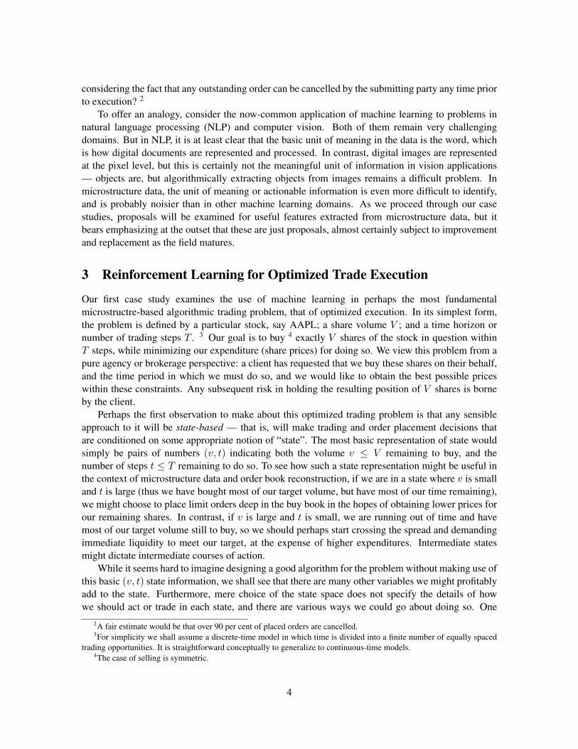
The potential promise of the learning approach is demonstrated by Figure 1. In this figure, wecompare the test set performance of the optimal one-shot strategy, and the policies learned by RL.To normalize price differences across stocks, we measure performance by implementation shortfall— namely, how much the average share price paid is greater than the midpoint of the spread at thebeginning of the trading period; thus, lower values are better. In the figure, we consider several valuesof the target volume and the period over which trading takes place, as well as both a coarser and finerchoice for how many discrete values we divide these quantities into in our state space representation(v, t). In every case we see that the performance of the RL policies is significantly better than theoptimal one-shot. We sensibly see that trading costs are higher overall for the higher target volumesand shorter trading periods. We also see that finer-grained discretization improves RL performance,an indicator that we have enough data to avoid overfitting from fragmenting our data across too largea state space.

Aside from the promising performance of the RL approach, it is instructive to visualize the de-tails of the actual policies learned, and is possible to do so in such a small, two-dimensional staterepresentation. Figure 2 shows examples of learned policies, where on the x and y axes, we indicatethe state (v, t) discretized into 8 levels each for both the number of trading steps remaining and theinventory (number of shares) left to purchase, and on the z axis, we plot the action learned by RLtraining relative to the top of the buy book (ask). Thus action ∆ corresponds to positioning our buyorder for the remaining shares at the bid plus ∆. Negative ∆ are orders placed down in the buy book,while positive ∆ enters or crosses the spread.

The learned policies are broadly quite sensible in the manner discussed earlier — when inventoryis high and time is running out, we cross the spread more aggressively; when inventory is low and mostof our time remains, we seek price improvement. But the numerical details of this broad landscapevary from stock to stock, and in our view this is the real value of machine learning in microstructureapplications — not in discovering “surprising” strategies per se, but in using large amounts of data

6 In principle we might compare our learning approach to state-of-the-art execution algorithms, such as the aforemen-tioned VWAP algorithms used by major brokerages. But doing so obscures the benefits of a principled learning approachin comparison to the extensive hand-tuning and optimization in industrial VWAP algorithms, and the latter may also makeuse of exotic order types, multiple exchanges, and other mechanisms outside of our basic learning framework. In practice,a combination of learning and hand-tuning would likely be most effective.

6

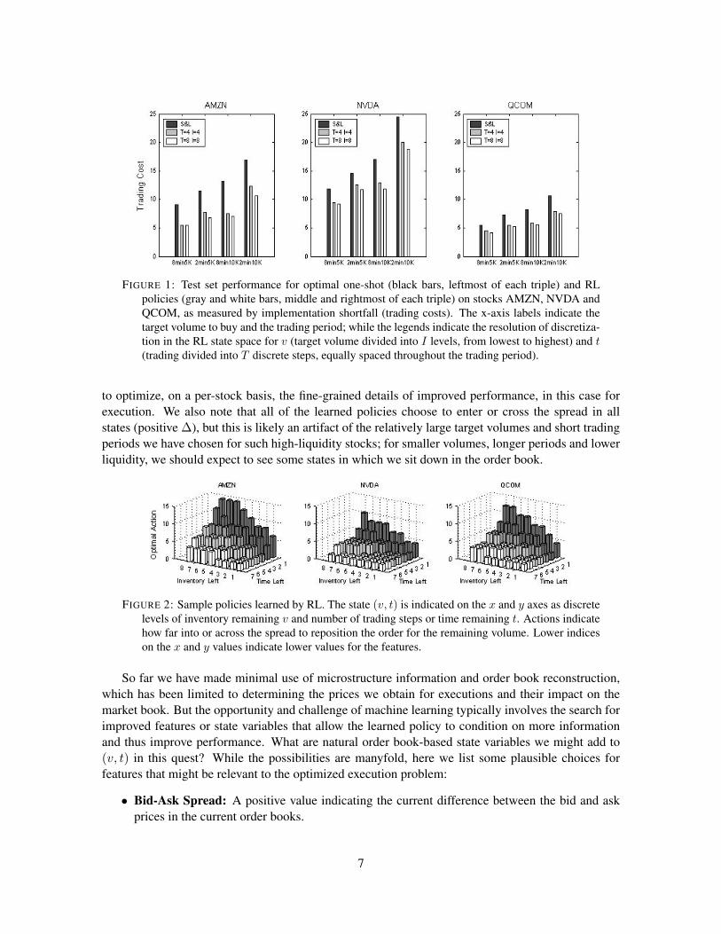
 FIGURE 1: Test set performance for optimal one-shot (black bars, leftmost of each triple) and RL

policies (gray and white bars, middle and rightmost of each triple) on stocks AMZN, NVDA andQCOM, as measured by implementation shortfall (trading costs). The x-axis labels indicate thetarget volume to buy and the trading period; while the legends indicate the resolution of discretiza-tion in the RL state space for v (target volume divided into I levels, from lowest to highest) and t(trading divided into T discrete steps, equally spaced throughout the trading period).

to optimize, on a per-stock basis, the fine-grained details of improved performance, in this case forexecution. We also note that all of the learned policies choose to enter or cross the spread in allstates (positive ∆), but this is likely an artifact of the relatively large target volumes and short tradingperiods we have chosen for such high-liquidity stocks; for smaller volumes, longer periods and lowerliquidity, we should expect to see some states in which we sit down in the order book.

 FIGURE 2: Sample policies learned by RL. The state (v, t) is indicated on the x and y axes as discrete

levels of inventory remaining v and number of trading steps or time remaining t. Actions indicatehow far into or across the spread to reposition the order for the remaining volume. Lower indiceson the x and y values indicate lower values for the features.

So far we have made minimal use of microstructure information and order book reconstruction,which has been limited to determining the prices we obtain for executions and their impact on themarket book. But the opportunity and challenge of machine learning typically involves the search forimproved features or state variables that allow the learned policy to condition on more informationand thus improve performance. What are natural order book-based state variables we might add to(v, t) in this quest? While the possibilities are manyfold, here we list some plausible choices forfeatures that might be relevant to the optimized execution problem:

• Bid-Ask Spread: A positive value indicating the current difference between the bid and askprices in the current order books.

7

• Bid-Ask Volume Imbalance: A signed quantity indicating the number of shares at the bidminus the number of shares at the ask in the current order books.

• Signed Transaction Volume: A signed quantity indicating the number of shares bought in thelast 15 seconds minus the number of shares sold in the last 15 seconds.

• Immediate Market Order Cost: The cost we would pay for purchasing our remaining sharesimmediately with a market order.

Along with our original state variables (v, t), the features above provide a rich language for dynami-cally conditioning our order placement on potentially relevant properties of the order books. For in-stance, for our problem of minimizing our expenditure for purchasing shares, perhaps a small spreadcombined with a strongly negative signed transaction volume would indicate selling pressure (sellerscrossing the spread, and filling in the resulting gaps with fresh orders). In such a state, depending onour inventory and time remaining, we might wish to be more passive in our order placement, sittingdeeper in the buy book in the hopes of price improvements.

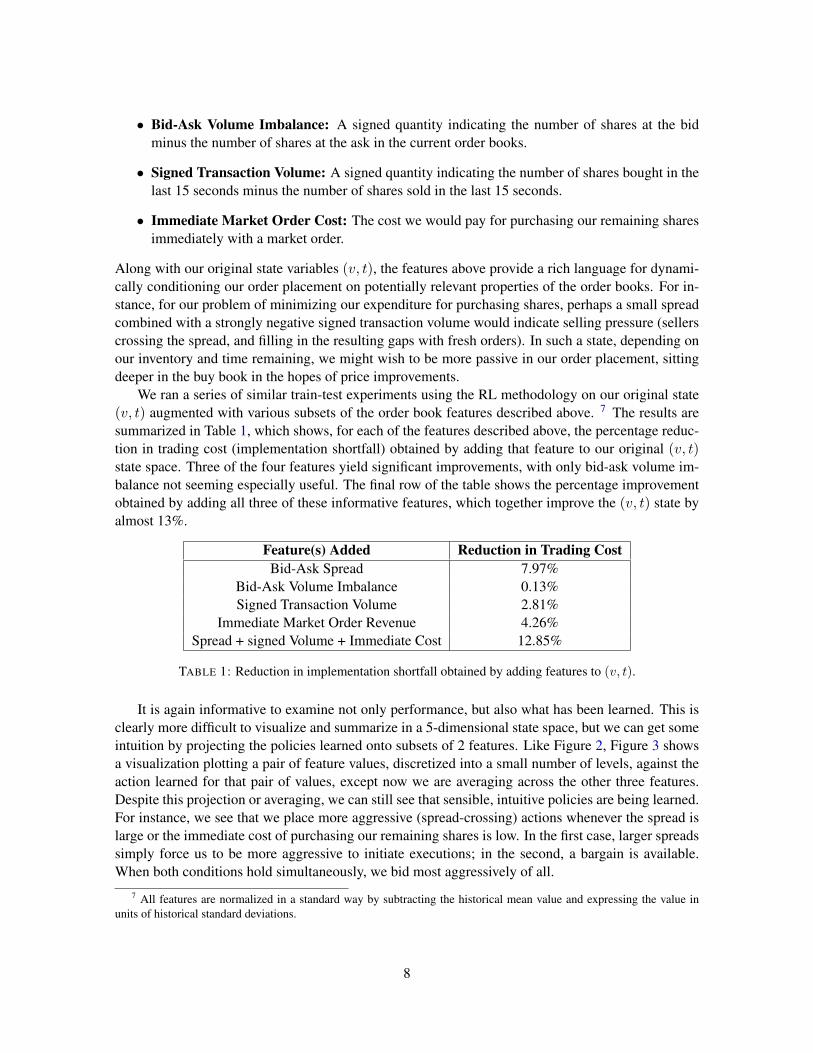
We ran a series of similar train-test experiments using the RL methodology on our original state(v, t) augmented with various subsets of the order book features described above. 7 The results aresummarized in Table 1, which shows, for each of the features described above, the percentage reduc-tion in trading cost (implementation shortfall) obtained by adding that feature to our original (v, t)state space. Three of the four features yield significant improvements, with only bid-ask volume im-balance not seeming especially useful. The final row of the table shows the percentage improvementobtained by adding all three of these informative features, which together improve the (v, t) state byalmost 13%.

Feature(s) Added Reduction in Trading CostBid-Ask Spread 7.97%

Bid-Ask Volume Imbalance 0.13%Signed Transaction Volume 2.81%

Immediate Market Order Revenue 4.26%Spread + signed Volume + Immediate Cost 12.85%

TABLE 1: Reduction in implementation shortfall obtained by adding features to (v, t).

It is again informative to examine not only performance, but also what has been learned. This isclearly more difficult to visualize and summarize in a 5-dimensional state space, but we can get someintuition by projecting the policies learned onto subsets of 2 features. Like Figure 2, Figure 3 showsa visualization plotting a pair of feature values, discretized into a small number of levels, against theaction learned for that pair of values, except now we are averaging across the other three features.Despite this projection or averaging, we can still see that sensible, intuitive policies are being learned.For instance, we see that we place more aggressive (spread-crossing) actions whenever the spread islarge or the immediate cost of purchasing our remaining shares is low. In the first case, larger spreadssimply force us to be more aggressive to initiate executions; in the second, a bargain is available.When both conditions hold simultaneously, we bid most aggressively of all.

7 All features are normalized in a standard way by subtracting the historical mean value and expressing the value inunits of historical standard deviations.

8

 FIGURE 3: Sample policies learned by RL for 5-feature state space consisting of (v, t) and three

additional order book features, projected onto the features of spread size and immediate cost topurchase remaining shares. Lower indices on the x and y values indicate lower values for thefeatures.

4 Predicting Price Movement from Order Book State

The case study of Section 3 demonstrated the potential of machine learning approaches to problems ofpure execution: we considered a highly constrained and stylized problem of reducing trading costs (inthis case, as measured by implementation shortfall), and showed that machine learning methodologycould provide important tools for such efforts.

It is of course natural to ask whether similar methodology can be fruitfully applied to the problemof generating profitable state-based models for trading using microstructure features. In other words,rather than seeking to reduce costs for executing a given trade, we would like to learn models thatthemselves profitably decide when to trade (that is, under what conditions in a given state space)and how to trade (that is, in which direction and with what orders), for alpha generation purposes.Conceptually (only) we can divide this effort into two components:

• The development of features that permit the reliable prediction of directional price movementsfrom certain states. By “reliable” we do not mean high accuracy, but just enough that ourprofitable trades outweigh our unprofitable ones.

• The development of learning algorithms for execution that capture this predictability or alphaat sufficiently low trading costs.

In other words, in contrast to Section 3, now we must first find profitable predictive signals, and thenhope they are not erased by trading costs. As we shall see, the former goal is relatively attainable,while the latter is relatively difficult.

It is worth remarking that for optimized execution in Section 3, we did not consider many featuresthat directly captured recent directional movements in execution prices; this is because the problemconsidered there exogenously imposed a trading need, and specified the direction and volume, somomentum signals were less important than those capturing potential trading costs. For alpha gen-eration, however, directional movement may be considerably more important. We thus conductedexperiments employing the following features:

• Bid-Ask Spread: Similar to that used in Section 3.

• Price: A feature measuring the recent directional movement of executed prices.

9

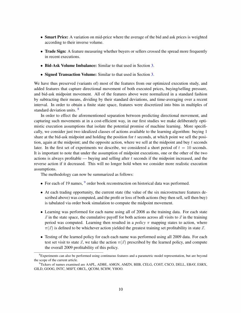
• Smart Price: A variation on mid-price where the average of the bid and ask prices is weightedaccording to their inverse volume.

• Trade Sign: A feature measuring whether buyers or sellers crossed the spread more frequentlyin recent executions.

• Bid-Ask Volume Imbalance: Similar to that used in Section 3.

• Signed Transaction Volume: Similar to that used in Section 3.

We have thus preserved (variants of) most of the features from our optimized execution study, andadded features that capture directional movement of both executed prices, buying/selling pressure,and bid-ask midpoint movement. All of the features above were normalized in a standard fashionby subtracting their means, dividing by their standard deviations, and time-averaging over a recentinterval. In order to obtain a finite state space, features were discretized into bins in multiples ofstandard deviation units. 8

In order to effect the aforementioned separation between predicting directional movement, andcapturing such movements at in a cost-efficient way, in our first studies we make deliberately opti-mistic execution assumptions that isolate the potential promise of machine learning. More specifi-cally, we consider just two idealized classes of actions available to the learning algorithm: buying 1share at the bid-ask midpoint and holding the position for t seconds, at which point we sell the posi-tion, again at the midpoint; and the opposite action, where we sell at the midpoint and buy t secondslater. In the first set of experiments we describe, we considered a short period of t = 10 seconds.It is important to note that under the assumption of midpoint executions, one or the other of the twoactions is always profitable — buying and selling after t seconds if the midpoint increased, and thereverse action if it decreased. This will no longer hold when we consider more realistic executionassumptions.

The methodology can now be summarized as follows:

• For each of 19 names, 9 order book reconstruction on historical data was performed.

• At each trading opportunity, the current state (the value of the six microstructure features de-scribed above) was computed, and the profit or loss of both actions (buy then sell, sell then buy)is tabulated via order book simulation to compute the midpoint movement.

• Learning was performed for each name using all of 2008 as the training data. For each state~x in the state space, the cumulative payoff for both actions across all visits to ~x in the trainingperiod was computed. Learning then resulted in a policy π mapping states to action, whereπ(~x) is defined to be whichever action yielded the greatest training set profitability in state ~x.

• Testing of the learned policy for each each name was performed using all 2009 data. For eachtest set visit to state ~x, we take the action π(~x) prescribed by the learned policy, and computethe overall 2009 profitability of this policy.

8Experiments can also be performed using continuous features and a parametric model representation, but are beyondthe scope of the current article.

9Tickers of names examined are AAPL, ADBE, AMGN, AMZN, BIIB, CELG, COST, CSCO, DELL, EBAY, ESRX,GILD, GOOG, INTC, MSFT, ORCL, QCOM, SCHW, YHOO.

10

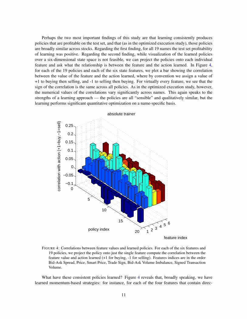
Perhaps the two most important findings of this study are that learning consistently producespolicies that are profitable on the test set, and that (as in the optimized execution study), those policiesare broadly similar across stocks. Regarding the first finding, for all 19 names the test set profitabilityof learning was positive. Regarding the second finding, while visualization of the learned policiesover a six-dimensional state space is not feasible, we can project the policies onto each individualfeature and ask what the relationship is between the feature and the action learned. In Figure 4,for each of the 19 policies and each of the six state features, we plot a bar showing the correlationbetween the value of the feature and the action learned, where by convention we assign a value of+1 to buying then selling, and -1 to selling then buying. For virtually every feature, we see that thesign of the correlation is the same across all policies. As in the optimized execution study, however,the numerical values of the correlations vary significantly across names. This again speaks to thestrengths of a learning approach — the policies are all “sensible” and qualitatively similar, but thelearning performs significant quantitative optimization on a name-specific basis.

1 2 3 4 5 6

0

5

10

15

20

−0.1

−0.05

0

0.05

0.1

0.15

0.2

0.25

feature index

absolute trainer

policy index

corr

elat

ion

with

act

ion

(+1=

buy,

−1=

sell)

FIGURE 4: Correlations between feature values and learned policies. For each of the six features and19 policies, we project the policy onto just the single feature compute the correlation between thefeature value and action learned (+1 for buying, -1 for selling). Features indices are in the orderBid-Ask Spread, Price, Smart Price, Trade Sign, Bid-Ask Volume Imbalance, Signed TransactionVolume.

What have these consistent policies learned? Figure 4 reveals that, broadly speaking, we havelearned momentum-based strategies: for instance, for each of the four features that contain direc-

11

tional information (Price, Smart Price, Trade Sign, Bid-Ask Volume Imbalance, and Signed Trans-action Volume), higher values of the feature (which all indicate either rising execution prices, risingmidpoints, or buying pressure in the form of spread-crossing) are accompanied by greater frequencyof buying in the learned policies. We should emphasize, however, that projecting the policies ontosingle features does not do justice to the subtleties of learning regarding interactions between the fea-tures. As just one simple example, if instead of conditioning on a single directional feature having ahigh value, we condition on several of them having high values, the correlation with buying becomesconsiderably stronger than for any isolated feature.

0 5 10 15 20−500

0

500

1000

1500

2000

2500

3000spread vs. all

0 5 10 15 20−500

0

500

1000

1500

2000

2500

3000price vs. all

0 5 10 15 20−2000

−1000

0

1000

2000

3000smartprice vs. all

0 5 10 15 200

500

1000

1500

2000

2500

3000

3500sign vs. all

0 5 10 15 20−3000

−2000

−1000

0

1000

2000

3000imbalance vs. all

0 5 10 15 200

500

1000

1500

2000

2500

3000volume vs. all

FIGURE 5: Comparison of test set profitability across 19 names for learning with all six features (redbars, identical in each subplot) versus learning with only a single feature (blue bars).

As we did for optimized execution, it is also instructive to examine which features are moremore or less informative or predictive of profitability. In Figure 5 there is a subplot for each of the sixfeatures. The red bars are identical in all six subplots, and show the test set profitability of the policies

12

learned for each of the 19 names when all six features are used. The blue bars in each subplot showthe test set profitability for each of the 19 names when only the corresponding single feature is used.General observations that can be made include:

• Profitability is usually better using all six features than any single feature.

• Smart Price appears to be the best single feature, and often is slightly better than using allfeatures together, a sign of mild overfitting in training. However, for one stock using all featuresis considerably better, and for another doing so avoids a significant loss from using Smart Priceonly.

• Spread appears to be the less useful single feature, but does enjoy significant solo profitabilityon a handful of names.

−3 −2 −1 0 1 2 3−4

−3

−2

−1

0

1

2

3x 10−8

state value

actio

n le

arne

d

(a) short term: momentum

−3 −2 −1 0 1 2 3−3

−2.5

−2

−1.5

−1

−0.5

0

0.5

1x 10−6

state value

actio

n le

arne

d

(b) medium term: reversion

−3 −2 −1 0 1 2 3−2

−1.5

−1

−0.5

0x 10−6

state value

(c) long term: directional drift

−3 −2 −1 0 1 2 3−3

−2

−1

0

1

2

3x 10−6

state value

actio

n le

arne

d

(d) long term, corrected: reversion

FIGURE 6: Learned policies depend strongly on timescale. For learning with a single feature measur-ing the recent directional price move, we show the test set profitability of buying in each possiblestate for varying holding periods.

While we see a consistent momentum relationship between features and actions across names,the picture changes when we explore different holding periods. Figure 6 illustrates how learning dis-covers different models depending on the holding period. We have selected a single “well-behaved”stock 10 (DELL) and plot value functions – which measure the test-set profits or losses — of a buy

10 The results we describe for DELL, however, do generalize consistently across names.

13

order in each possible state of a single-feature state space representing recent price changes. 11 Notethat since executions take place at the midpoints, the value functions for selling are exactly oppositethose shown. We show the value function for several different holding periods.

Over very short holding periods (see Figure 6(a)), we see fairly consistent momentum behavior:for time periods of milliseconds to seconds, price moves tend to continue. At these time scales, buyingis (most) profitable when the recent price movements have been (strongly) upwards, and unprofitablewhen the price has been falling. This echoes the consistency of learned multi-feature momentumstrategies described above, which were all at short holding. Features that capture directional movesare positively correlated with future returns: increasing prices, preponderance of buy trades, andhigher volumes in the buy book all forecast higher returns in the immediate future.

We see a different pattern, however, when examining longer holding periods (dozens of secondsto several minutes). At those horizons, (see Figure 6(b)), our learner discovers reversion strategies:buying is now profitable under recent downward price movements, and selling is profitable after up-ward price movements. Again, these results are broadly consistent across names and related features.

A desirable property of a “good fit” in statistical learning is to have models with features thatpartition the variable that they aim to predict into distinct categories. Our short-term momentum andlonger-term reversion strategies exhibit such behavior: in the momentum setting, the highest val-ues of past returns predict the highest future returns, and the most negative past returns imply themost negative subsequent realizations (and vice-versa for reversion). Furthermore, this relationshipis monotonic, with past returns near zero corresponding to near-zero future returns: in Figure 6(a)and (b) the most pronounced bars are the extremal ones. We lose this desirable monotonicity, how-ever, when extending our holding period even further: in the range of 30 minutes to several hours,conditioning on any of our chosen variables no longer separates future positive and negative returns.Instead, we end up just capturing the overall price movement or directional drift – as demonstrated inFigure 6(c), the expected value of a buy action has the same (negative) sign across all states, and isdistributed more uniformly, being roughly equal to the (negative) price change over the entire trainingperiod (divided by the number of training episodes). Thus since the price went down over the courseof the training period, we simply learn to sell in every state, which defeats the purpose of learning adynamic state-dependent strategy.

The discussion so far highlights the two aspects that one must consider when applying machinelearning to high frequency data: the nature of the underlying price formation process, and the roleand limitations of the learning algorithm itself. In the first category, a clean picture of market me-chanics emerges: when we look at price evolution over milliseconds to seconds, we likely witnesslarge marketable orders interacting with the order book, creating directional pressure. Over severalminutes, we see the flip side of this process: when liquidity demanders push prices too far from theirequilibrium state, reversion follows. On even longer time scales, our microstructure-based variablesare less informative, apparently losing their explanatory power.

On one hand, it may be tempting to simply conclude that for longer horizons microstructurefeatures are immaterial to the price formation process, but longer holding periods are of a particularinterest to us. As we have pointed out in our HFT profitability study [9], there is a tension betweenshorter holding periods and the ability to overcome trading costs (specifically, the bid-ask spread).While the direction of price moves is easiest to forecast over the very short intervals, the magnitudeof these predictions – and thus the margin that allows one to cover trading costs – grows with holding

11As usual, the feature is normalized by subtracting the mean and binned by standard deviations, so -3 means the recentprice change is 3 standard deviations below its historical mean, and +3 means it is three standard deviations above.

14

periods (notice that the scale of the y axis, which is measuring profitability, is 100 times larger inFigure 6(b) than in Figure 6(a)). Ideally, we would like to find some compromise horizon, which islong enough to allow prices to evolve sufficiently in order to beat the spread, but short enough formicrostructure features to be informative of directional movements.

In order to reduce the influence of any long-term directional price drift, we can adjust the learningalgorithm to account for it. Instead of evaluating the total profit per share or return from a buy actionin a given state, we monitor the relative profitability of buying in that state versus buying in everypossible state. For example, suppose a buy action in state S yields 0.03 cents per trade on average;while that number is positive, suppose always buying (that is, in every state) generates 0.07 cents pertrade on average (presumably because the price went up over the course of the entire period), thereforemaking state s relatively less advantageous for buying. We would then assign −0.04 = 0.03 − 0.07as the value of buying in that state. Conversely, there may be a state-action pair that has negativepayout associated with it over the training period, but if this action is even more unprofitable whenaveraged across all states (again, presumably due to a long-term price drift), this state-action pair beassigned a positive value. Conceptually, such “adjustment for average value” allows us to filter out theprice trend and hone in on microstructure aspects, which also makes learned policies perform morerobustly out-of-sample. Empirically, resulting learned policies recover the desired symmetry, whereif one extremal state learns to buy, the opposite extremal state learns to sell – notice the transformationfrom Figure 6(c) to Figure 6(d), where we once again witness mean reversion.

While we clearly see patterns in the short-term price formation process and are demonstrativelysuccessful in identifying state variables that help predict future returns, profiting from this predictabil-ity is far from trivial. It should be clear from the figures in this section that the magnitude of ourpredictions is in fractions of a penny, whereas the tightest spread in liquid US stocks is one cent.So in no way should the results be interpreted as a recipe for profitability: even if all the featureswe enumerate here are true predictors of future returns, and even if all of them line up just right formaximum profit margins, one still cannot justify trading aggressively and paying the bid-ask spread,since the magnitude of predictability is not sufficient to cover transaction costs. 12

So what can be done? We see essentially three possibilities. First, as we have suggested earlier,we could hold our positions longer, so that price changes are larger than spreads, giving us highermargins. However, as we have seen, the longer the holding period, the less directly informativemarket microstructure aspects seem to become, thus making prediction more difficult. Second, wecould trade with limit orders, hoping to avoid paying the spread. This is definitely a fruitful direction,where one jointly estimates future returns and the probability of getting filled, which then must beweighed against adverse selection (probability of executing only when predictions turn out to bewrong). This is a much harder problem, well outside of the scope of this article. And finally, athird option is to find or design better features that will bring about greater predictability, sufficient toovercome transaction costs.

It should be clear now that the overarching theme of these suggested directions is that the machinelearning approach offers no easy paths to profitability. Markets are competitive, and finding sourcesof true profitability is extremely difficult. That being said, what we have covered in this section isa framework for how to look for sources of potential profits in a principled way – by defining statespaces, examining potential features and their interplay, using training-test set methodology, imposingsensible value functions, etc – that should be a part of the arsenal of a quantitative professional, sothat we can at least discuss these problems in a common language.

12Elsewhere we have documented this tension empirically at great length [9].

15

5 Machine Learning for Smart Order Routing in Dark Pools

The studies we have examined so far apply machine learning to trading problems arising in relativelylong-standing exchanges (the open limit order book instantiation of a continuous double auction),where microstructure data has been available for some time. Furthermore, this data is rich — showingthe orders and executions for essentially all market participants, comprising multiple order types, andso on — and is also extremely voluminous. In this sense these exchanges and data are ideal testbedsfor machine learning for trading, since (as we have seen) they permit the creation of rich featurespaces for state-based learning approaches.

But machine learning methodology is also applicable to recently emerging exchanges, with newmechanisms and with data that is considerably less rich and voluminous. For our final case study,we describe the use of a machine learning approach to the problem of Smart Order Routing (SOR) indark pools. Whereas our first study investigated reinforcement learning for the problem of dividinga specified trade across time, here we examine learning to divide a specified trade across venues —that is, multiple competing dark pools, each offering potentially different liquidity profiles. Beforedescribing this problem in greater detail, we first provide some basic background on dark pools andtheir trade execution mechanism.

Dark pools were originally conceived as a venue for trades in which liquidity is of greater concernthan price improvement — for instance, trades whose volume is sufficiently high that executing in thestandard lit limit order exchanges (even across time and venues) would result in unacceptably hightrading costs and market impact. For such trades, one would be quite satisfied to pay the “currentprice” — say, as measured by the bid-ask midpoint — as long as there were sufficiently liquidity todo so. The hope is that dark pools can perhaps match such large-volume counterparties away fromthe lit exchanges.

In the simplest form of dark pool mechanism, orders simply specify the desired volume for agiven name, and the direction of trade (buy or sell); no prices are specified. Orders are queued ontheir respective side of the market in order of their arrival, with the oldest orders at the front of thequeue. Any time there is liquidity on both sides of the market, execution occurs. For instance, supposeat a given instant the buy queue is empty, and the sell queue consists of two orders for 1000 and 250shares. If a new buy order arrives for 1600 shares, it will immediately be executed for 1250 sharesagainst the outstanding sell orders, after which the buy queue will contain the order for the residual350 shares and the sell queue will be empty. A subsequent arrival of a buy order for 500 shares,followed by a sell order for 1000 shares, will result in an empty buy queue and the residual sell orderfor 150 (= 1000 − 350 − 500) shares. Thus at any instant, either one or both of the buy and sellqueues will be empty, since incoming orders are either added to the end of the non-empty queue, orcause immediate execution with the other side. In this sense, all orders are “market” orders, in thatthey express a demand for immediate liquidity.

At what prices do the executions take place, since orders do not specify prices? As per theaforementioned motivation of liquidity over price (improvement), in general dark pool executionstake place at the prevailing prices in the corresponding lit (limit order) market for the stock in question– for instance, at the midpoint of the bid-ask spread, as measured by the National Best Bid and Offer(NBBO). Thus while dark pools operate separately and independently of the lit markets, their pricesare strongly tied to those lit markets.

From a data and machine learning perspective, there are two crucial differences between darkpools and their lit market counterparts:

16

• Unlike the microstructure data for the lit markets, in dark pools one has access only to one’sown order and execution data, rather than the entire trading population. Thus the rich fea-tures measuring market activity, buying and selling pressure, liquidity imbalances, etc. that weexploited in Sections 3 and 4 are no longer available.

• Upon submitting an order to a dark pool, all we learn is whether our order has been (partially)executed, not how much liquidity might have been available had we asked for more. For in-stance, suppose we submit an order for 10,000 shares. If we learn that 5,000 shares of it havebeen executed, then we know that only 5,000 shares were present on the other side. However,if all 10,000 shares have been executed, then any amount larger than 10,000 might have beenavailable. More formally, if we submit an order for V shares and S shares are available, welearn only the value min(V, S), not S. In statistics this is known as censoring. We shall seethat the machine learning approach we take to order routing in dark pools explicitly accountsfor censored data.

These two differences mean that dark pools provide us with considerably less information not onlyabout the activity of other market participants, but even about the liquidity present for our own trades.Nevertheless, we shall see there is still a sensible and effective machine learning approach.

We are now ready to define the SOR problem more mathematically. We assume that there are nseparate dark pools available (as of this writing n > 30 in the United States alone), and we assumethat these pools may offer different liquidity profiles for a given stock — for instance, one pool maybe better at reliably executing small orders quickly, while another may have a higher probability ofexecuting large orders. We model these liquidity profiles by probability distributions over availableshares. More precisely, let Pi be a probability distribution over the non-negative integers. We assumethat upon submitting an order for Vi shares to pool i, a random value Si is drawn according to Pi;Si models the shares available on the other side of the market of our trade (selling if we are buying,buying if we are selling) at the moment of submission. Thus as per the aforementioned mechanism,min(Vi, Si) shares will be executed. The SOR problem can now be formalized as follows: givenan overall target volume V we would like to (say) buy, how should we divide V into submissionsV1, . . . , Vn to the n dark pools such that

∑ni=1 Vi = V , and we maximize the (expected) number of

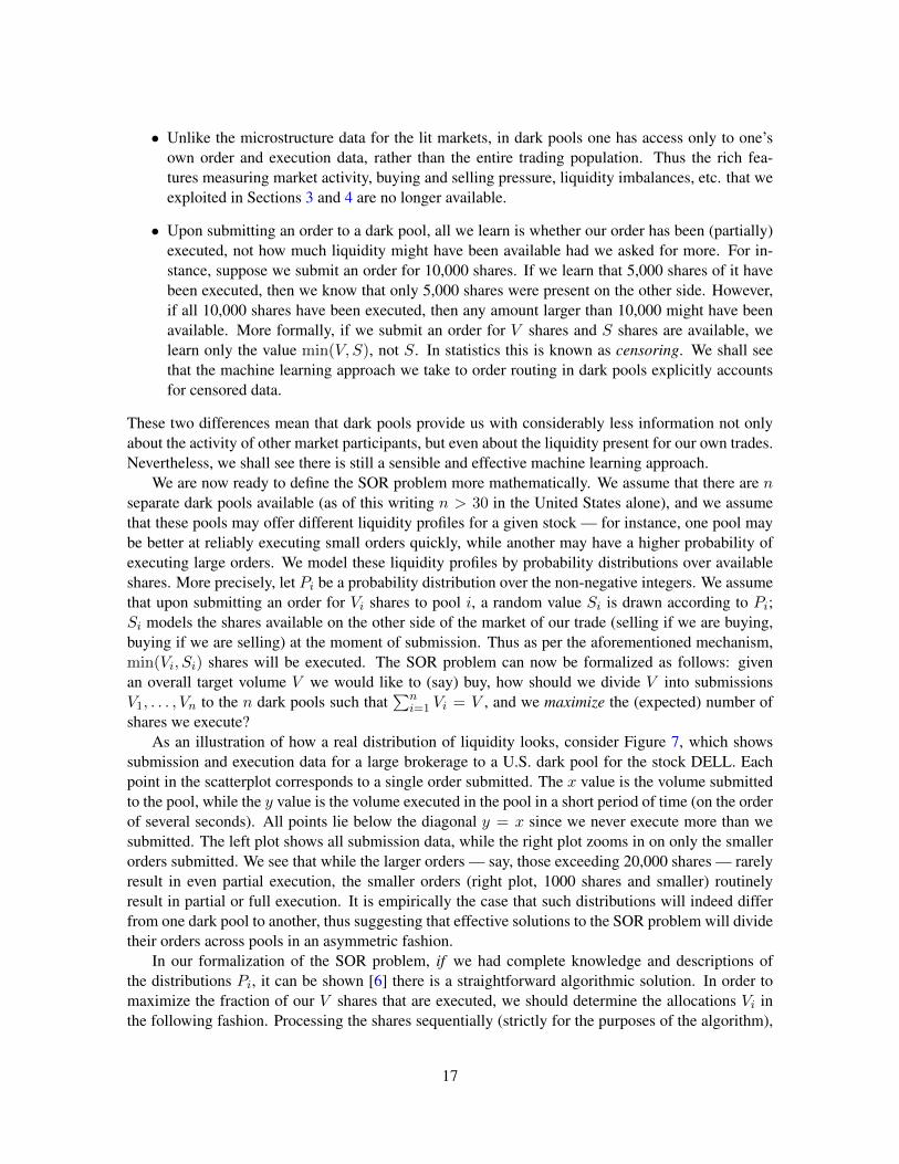
shares we execute?As an illustration of how a real distribution of liquidity looks, consider Figure 7, which shows

submission and execution data for a large brokerage to a U.S. dark pool for the stock DELL. Eachpoint in the scatterplot corresponds to a single order submitted. The x value is the volume submittedto the pool, while the y value is the volume executed in the pool in a short period of time (on the orderof several seconds). All points lie below the diagonal y = x since we never execute more than wesubmitted. The left plot shows all submission data, while the right plot zooms in on only the smallerorders submitted. We see that while the larger orders — say, those exceeding 20,000 shares — rarelyresult in even partial execution, the smaller orders (right plot, 1000 shares and smaller) routinelyresult in partial or full execution. It is empirically the case that such distributions will indeed differfrom one dark pool to another, thus suggesting that effective solutions to the SOR problem will dividetheir orders across pools in an asymmetric fashion.

In our formalization of the SOR problem, if we had complete knowledge and descriptions ofthe distributions Pi, it can be shown [6] there is a straightforward algorithmic solution. In order tomaximize the fraction of our V shares that are executed, we should determine the allocations Vi inthe following fashion. Processing the shares sequentially (strictly for the purposes of the algorithm),

17

0 2 4 6 8 10

x 104

0

1

2

3

4

5

6

7

8

9

10x 104

volu

me

fille

d

volume submitted

all orders

0 200 400 600 800 10000

100

200

300

400

500

600

700

800

900

1000

volu

me

fille

d

volume submitted

small orders

FIGURE 7: Sample submission and execution data for DELL from a large brokerage firm orders to aU.S. dark pool. The x axis shows the volume submitted, and the y value the volume executed in ashort period following submission. Points on the diagonal correspond to censored observations.

we allocate the conceptually “first” share to whichever pool has the highest probability of executing asingle share. Then inductively, if we have already determined a partial allocation of the V shares, weshould allocate our “next” share to whichever pool has the highest marginal probability of executingthat share, conditioned on the allocation made so far. In this manner we process all V shares anddetermine the resulting allocation Vi for each pool i. We shall refer to this algorithm for makingallocations under known Pi the greedy allocation algorithm. It can be shown that the greedy allocationalgorithm is an optimal solution to the SOR problem, in that it maximizes the expected number ofshares executed in a single round of submissions to the n pools. Note that if the submission of our Vshares across the pools results in partial executions leaving us with V ′ < V shares remaining, we canalways repeat the process, resubmitting the V ′ shares in the allocations given by the greedy algorithm.

The learning problem for SOR arises from the fact that we do not have knowledge of the distribu-tions Pi, and must learn (approximations to) them from only our own, censored order and executiondata — that is, data of the form visualized in Figure 7. We have developed an overall learning algo-rithm for the dark pool SOR problem that learns an optimal submission strategy over a sequence ofsubmitted volumes to the n venues. The details of this algorithm are beyond the current scope, butcan be summarized as follows:

• The algorithm maintains, for each venue i, an approximation P̂i to the unknown liquidity dis-tribution Pi. This approximation is learned exclusively from the algorithm’s own order sub-mission and execution data to that venue. Initially, before any orders have been submitted, allof the approximations P̂i have some default form.

• Since the execution data is censored by our own submitted volume, we cannot employ basicstatistical methods for estimating distributions from observed frequencies. Instead, we usethe Kaplan-Meier estimator (sometimes also known as the product limit estimator), which isthe maximum likelihood estimator for censored data [6] . Furthermore, since empirically theexecution data exhibits and overwhelming incidence of no shares executed, combined withoccasional executions of large volumes (see Figure 7), we adapt this estimator for a parametricmodel for the P̂i that has the form of a power law with a separate parameter for zero shares.

18

• For each desired volume V to execute, the algorithm simply behaves as if its current approx-imate distributions P̂i are in fact the true liquidity distributions, and chooses the allocationsVi according to the greedy algorithm applied to the P̂i. Each submitted allocation Vi then re-sults in an observed volume executed (which could be anything from zero shares to a censoredobservation of Vi shares).

• With this fresh execution data, the estimated distributions P̂i can be updated, and the processrepeated for the next target volume.

In other words, the algorithm can be viewed as a simple repeated loop of optimization followedby re-estimation: our current distributional estimates are inputs to the greedy optimization, whichdetermines allocations, which result in executions, which allow us to estimate improved distributions.It is possible, under some simple assumptions, to prove that this algorithm will rapidly converge tothe optimal submission strategy for the unknown true distributions Pi. Furthermore the algorithm iscomputationally very simple and efficient, and variants of it have been implemented in a number ofbrokerage firms.

0 500 1000 1500 20000.06

0.065

0.07

0.075

0.08

0.085

0.09

0.095

0.1

0.105

0.11

episodes

fract

ion

exec

uted

Ticker = XOM, Volume = 8000, Trials = 800, Smoothing = 0.99

0 500 1000 1500 2000

0.13

0.14

0.15

0.16

0.17

0.18

0.19

episodes

fract

ion

exec

uted

Ticker = AIG, Volume = 8000, Trials = 800, Smoothing = 0.99

0 500 1000 1500 20000.08

0.085

0.09

0.095

0.1

0.105

0.11

0.115

0.12

episodes

fract

ion

exec

uted

Ticker = NRG, Volume = 8000, Trials = 800, Smoothing = 0.99

FIGURE 8: Performance curves for our learning algorithm (red) and a simple adaptive heuristic (blue),against benchmarks measuring uniform allocations (black) and ideal allocations (green).

Some experimental validation of the algorithm is provided in Figure 8, showing simulations de-rived using the censored execution data for four U.S. dark pools. Each subplot shows the evolutionof our learning algorithm’s performance on a series of submitted allocations for a given ticker to thepools. The x axis measures time or trials for the algorithm — that is, the value of x is the number ofrounds of submitted volumes so far. The y axis measures the total fraction of the submitted volumethat was executed across the four pools; higher values are thus better. The red curves for each nameshow the performance of our learning algorithm. In each case performance improves rapidly withadditional rounds of allocations, as the estimates P̂i become better approximations to the true Pi.

As always in machine learning, it is important to compare our algorithm’s performance to somesensible benchmarks and alternatives. The least challenging comparison is shown by the black hor-izontal line in each figure, which represents the expected fraction of shares executed if we simplydivide every volume V equally amongst the pools — thus there is no learning, and no accountingfor the asymmetries that exist amongs the venues. Fortunately we see the learning approach quicklysurpasses this sanity-check benchmark.

A more challenging benchmark is the horizontal green line in each subplot, which shows theexpected fraction of shares executed when performing allocations using the greedy algorithm appliedto the true distributions Pi. This is the best performance we could possibly hope to achieve, and wesee that our learning algorithm approaches this ideal quickly for each stock.

19

Finally, we compare the learning algorithm’s performance to a simple adaptive algorithm thatis a “poor man’s” form of learning. Rather than maintaining estimates of the complete liquiditydistribution for each venue i, it simply maintains a single numerical weight wi, and allocates Vproportional to thewi. If a submission to venue i results in any shares being executed, wi is increased;otherwise it is decreased. We see that while in some cases this algorithm can also approach the trueoptimal, in other cases it asymptotes at a suboptimal value, and in others it seems to outright divergefrom optimality. In each case our learning algorithm outperforms this simple heuristic.

6 Conclusions

In this article we have presented both the opportunities and challenges of a machine learning approachto HFT and market microstructure. We have considered both problems of pure execution, over bothtime and venues, and predicting directional movements in search of profitability. These were illus-trated via three detailed empirical case studies. In closing, we wish to emphasize a few “lessonslearned” common to all of the cases examined:

• Machine learning provides no easy paths to profitability or improved execution, but does pro-vide a powerful and principled framework for trading optimization via historical data.

• We are not believers in the use of machine learning as a black box, nor the discovery of “sur-prising” strategies via its application. In each of the case studies, the result of learnings madebroad economic and market sense in light of the trading problem considered. However, thenumerical optimization of these qualitatitve strategies is where the real power lies.

• Throughout we have emphasized the importance and subtlety of feature design and engineeringto the success of the machine learning approach. Learning will never succeed without informa-tive features, and may even fail with them if they are not expressed or optimized properly.

• All kinds of other fine-tuning and engineering are required to obtain the best results, such asthe development of learning methods that correct for directional drift in Section 4.

Perhaps the most important overarching implication of these lessons is that there will always bea “human in the loop” in machine learning applications to HFT (or any other long-term effort toapply machine learning to a challenging, changing domain). But applied tastefully and with care, theapproach can be powerful and scalable, and is arguably necessary in the presence of microstructuredata of such enormous volume and complexity as confronts us today.

Acknowledgements

We give warm thanks to Alex Kulesza for his collaboration on the research described in Section 4,and to Frank Corrao for his valuable help on many of our collaborative projects.

References

[1] A. Agarwal, P. Bartlett, and M. Dama. Optimal Allocation Strategies for the Dark Pool Problem.Technical Report, arXiv.org, 2010.

20

[2] D. Bertsimas and A. Lo. Optimal Control of Execution Costs. J. Financial Markets, 1(1), 1998.

[3] J. Bouchaud, M. Mezard, and M. Potters. Statistical Properties of Stock Order Books: EmpiricalResults and Models. Quantitative Finance, 2:251–256, 2002.

[4] R. Cont and A. Kukanov. Optimal Order Placement in Limit Order Markets. Technical Report,arXiv.org, 2013.

[5] E. Fama and K. French. Common Risk Factors in the Returns on Stocks and Bonds. Journal offinancial economics, 33(1):3–56, 1993.

[6] K. Ganchev, M. Kearns, Y. Nevmyvaka, and J. Wortman. Censored Exploration and the DarkPool Problem. Communications of the ACM, 53(5):99–107, 2010.

[7] O. Guant, C.A. Lehalle, and J.F. Tapia. Optimal Portfolio Liquidation with Limit Orders. Tech-nical Report, arXiv.org, 2012.

[8] I. Kharroubi and H. Pham. Optimal Portfolio Liquidation with Execution Cost and Risk. SIAMJournal on Financial Mathematics, 1(1), 2010.

[9] A. Kulesza, M. Kearns, and Y. Nevmyvaka. Empirical Limitations on High Frequency TradingProfitability. Journal of Trading, 5(4):50–62, 2010.

[10] S. Laruelle, C.A. Lehalle, and G. Pages. Optimal Split of Orders Across Liquidity Pools : AStochastic Algorithm Approach. SIAM Journal on Financial Mathematics, 2(1), 2011.

[11] C. Maglaras, C. C. Moallemi, and H. Zheng. Optimal Order Routing in a Fragmented Market.Working paper, 2012.

[12] C. C. Moallemi, B. Park, and B. Van Roy. Strategic Execution in the Presence of an UninformedArbitrageur. Journal of Financial Markets, 15(4):361391, 2012.

[13] JP Morgan. Dark Matters Part 1: Optimal Liquidity Seeker (JP Morgan Electronic Client Solu-tions). May 2012.

[14] Yuriy Nevmyvaka, Yi Feng, and Michael Kearns. Reinforcement Learning for Optimized TradeExecution. In Proceedings of the 23rd international conference on Machine learning, pages673–680. ACM, 2006.

[15] B. Park and B. Van Roy. Adaptive Execution: Exploration and Learning of Price Impact. Tech-nical Report, arXiv.org, 2012.

[16] Richard S. Sutton and Andrew G. Barto. Reinforcement Learning: An Introduction. MIT Press,1998.

21