MA162: Finite mathematicsLinear Programming: More on Method of Corners

Paul Koester

University of Kentucky

April 21, 2014

Schedule:

Overview

Last class, we introduced the method of corners.

Today, we look at the four main steps1 Step 1: Graph the lines2 Step 2: Deal with inequalities3 Step 3: Find the corners4 Step 4: Evaluate objective on the corners

We will look at a rather lengthy example. We will illustratethe basic flavor of each of the above steps, but we will skipover a lot of the computations. The computations are includedin this set of notes. To get the most out of this example,

After class, try to complete all of the steps on your own.Refer to these slides for the details

We will also talk about the advantages and disadvantages ofthe method of corners.

Example

Maximize the linear function

f (x , y) = 2x + 3y − 1

subject to the constraints

3x − y ≥ −1

x + y ≤ 7

x + 2y ≤ 10

−x + 4y ≥ 0

x − y ≤ 3

x ≥ 0

0 ≤ y ≤ 4

Step 1: Graph each equality

For an individual inequality, start with the equality:

3x − y = −1

Since this line is not vertical, not horizontal, nor passes through(0, 0), we should find its x and y intercepts.x-intercept: y = 0 implies 3x − 0 = −1 implies x = −1/3.y -intercept: x = 0 implies 3 · 0 − y = −1 implies y = 1.

(−1/3, 0)

(0, 1)

3x − y = −1

Step 1: Graph each equality

The fourth constraint is −x + 4y ≥ 0. The corresponding equalityis −x + 4y = 0. The x and y intercepts are each 0. This isinsufficient information to plot the line. Instead, rewrite asy = (1/4)x . This is a line through the origin and with slope 1/4.

3x − y = −1

−x + 4y = 0

Step 1: Graph each equality

In a similar way, we graph each of the remaining constraints.3x − y = −1

−x + 4y = 0

x + y = 7

x + 2y = 10

x − y = 3

y = 4

y = 0

x = 0

Step 2: Deal with the INequalites

3x − y ≥ −1

−x + 4y ≥ 0

x + y ≤ 7

x + 2y ≤ 10

x − y ≤ 3

y ≤ 4

y ≥ 0

x ≥ 0

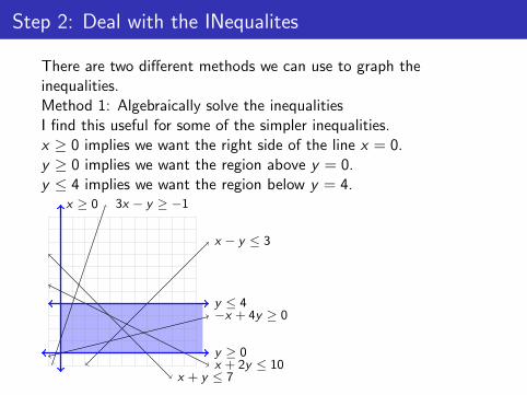
Step 2: Deal with the INequalites

There are two different methods we can use to graph theinequalities.Method 1: Algebraically solve the inequalitiesI find this useful for some of the simpler inequalities.x ≥ 0 implies we want the right side of the line x = 0.y ≥ 0 implies we want the region above y = 0.y ≤ 4 implies we want the region below y = 4.

3x − y ≥ −1

−x + 4y ≥ 0

x + y ≤ 7x + 2y ≤ 10

x − y ≤ 3

y ≤ 4

y ≥ 0

x ≥ 0

Step 2: Deal with the INequalites

This also works well for inequalities in which the coefficients of xand y are both positive.x + y ≤ 7 implies region on bottom left of x + y = 7x + 2y ≤ 10 implies region on bottom left of x + 2y = 10

3x − y ≥ −1

−x + 4y ≥ 0

x + y ≤ 7x + 2y ≤ 10

x − y ≤ 3

y ≤ 4

y ≥ 0

x ≥ 0

Step 2: Deal with the INequalites

If the coefficients of x and y have opposite signs, solve for y.x − y ≤ 3 implies y ≥ x − 3. Think of this as saying y is large. Wewant region above x − y = 3.

3x − y ≥ −1

−x + 4y ≥ 0

x + y ≤ 7

x + 2y ≤ 10

x − y ≤ 3

y ≤ 4

y ≥ 0

x ≥ 0

Step 2: Deal with the INequalites

Similarly, −x + 4y ≥ 0 rearranges to y ≥ x/4.Think of this as saying y is large, so we want region abovex − 4y = 0.

3x − y ≥ −1

−x + 4y ≥ 0

x + y ≤ 7

x + 2y ≤ 10

x − y ≤ 3

y ≤ 4

y ≥ 0

x ≥ 0

Step 2: Deal with the INequalites

Finally, 3x − y ≥ −1 rearranges to y ≤ 3x + 1.Think of this as saying y should be small, so want region belowy = 3x + 1.

3x − y ≥ −1

−x + 4y ≥ 0

x + y ≤ 7

x + 2y ≤ 10

x − y ≤ 3

y ≤ 4

y ≥ 0

x ≥ 0

Step 2: Deal with the INequalites

We have found the correct region. The next step is to find thecorners of the region.

3x − y ≥ −1

−x + 4y ≥ 0

x + y ≤ 7

x + 2y ≤ 10

x − y ≤ 3

y ≤ 4

y ≥ 0

x ≥ 0

Step 3: Finding the Corners

Since we have a nice computer generated plot and all of thecorners appear to have integer coefficients, we can easily read offthe corners.However, we won’t always have such nice graphs, so how can wefind the corner points in general?Each corner point arises by intersecting a pair of the lines.Notice, however, that not all intersection points are corners of theshaded region.Use the shaded region to help determine which pairs of lines needto be intersected.

Step 3: Finding the Corners, First Point

3x − y ≥ −1

−x + 4y ≥ 0

x + y ≤ 7

x + 2y ≤ 10

x − y ≤ 3

y ≤ 4

y ≥ 0

x ≥ 0

The red corner is obtained by intersection the red lines,

x + y = 7x + 2y = 10[

1 1 71 2 10

]R2 7→R2−R1−−−−−−−→

[1 1 70 1 3

]R1 7→R1−R2−−−−−−−→

[1 0 40 1 3

]So the red corner point is (x , y) = (4, 3)

Step 3: Finding the Corners, Second Point

3x − y ≥ −1

−x + 4y ≥ 0

x + y ≤ 7

x + 2y ≤ 10

x − y ≤ 3

y ≤ 4

y ≥ 0

x ≥ 0

The red corner is obtained by intersection the red lines,x + y = 7x − y = 3[

1 1 71 −1 3

]R2 7→R2−R1−−−−−−−−→

[1 1 70 −2 −4

]R2 7→R2/−2−−−−−−−−→

[1 1 70 1 2

]R1 7→R1−R2−−−−−−−−→

[1 0 50 1 2

]

So the red corner point is (x , y) = (5, 2)

Step 3: Finding the Corners, Third Point

3x − y ≥ −1

−x + 4y ≥ 0

x + y ≤ 7

x + 2y ≤ 10

x − y ≤ 3

y ≤ 4

y ≥ 0

x ≥ 0

The red corner is obtained by intersection the red lines,x − y = 3−x + 4y = 0[

1 −1 3−1 4 0

]R2 7→R2+R1−−−−−−−−→

[1 −1 30 3 3

]R2 7→R2/3−−−−−−−→

[1 −1 30 1 1

]R1 7→R1+R2−−−−−−−−→

[1 0 40 1 1

]

So the red corner point is (x , y) = (4, 1)

Step 3: Finding the Corners, Fourth Point

3x − y ≥ −1

−x + 4y ≥ 0

x + y ≤ 7

x + 2y ≤ 10

x − y ≤ 3

y ≤ 4

y ≥ 0

x ≥ 0

The red corner is obtained by intersection the red lines,x = 0−x + 4y = 0[

1 0 0−1 4 0

]R2 7→R2+R1−−−−−−−−→

[1 0 00 4 0

]R2 7→R2/4−−−−−−−→

[1 0 00 1 0

]

So the red corner point is (x , y) = (0, 0)

Step 3: Finding the Corners, Fifth Point

3x − y ≥ −1

−x + 4y ≥ 0

x + y ≤ 7

x + 2y ≤ 10

x − y ≤ 3

y ≤ 4

y ≥ 0

x ≥ 0

The red corner is obtained by intersection the red lines,x = 03x − y = −1[

1 0 03 −1 −1

]R2 7→R2−3R1−−−−−−−−−→

[1 0 00 −1 −1

]R2 7→−R2−−−−−−→

[1 0 00 1 1

]

So the red corner point is (x , y) = (0, 1)

Step 3: Finding the Corners, Sixth Point

3x − y ≥ −1

−x + 4y ≥ 0

x + y ≤ 7

x + 2y ≤ 10

x − y ≤ 3

y ≤ 4

y ≥ 0

x ≥ 0

The red corner is obtained by intersection the red lines,3x − y = −10 y = 4[

3 −1 −10 1 4

]R1 7→R1+R2−−−−−−−−→

[3 0 30 1 4

]R1 7→R1/3−−−−−−−→

[1 0 10 1 4

]

So the red corner point is (x , y) = (1, 4)

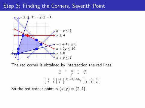
Step 3: Finding the Corners, Seventh Point

3x − y ≥ −1

−x + 4y ≥ 0

x + y ≤ 7

x + 2y ≤ 10

x − y ≤ 3

y ≤ 4

y ≥ 0

x ≥ 0

The red corner is obtained by intersection the red lines,x + 2y = 100 y = 4[

1 2 100 1 4

]R1 7→R1−2R2−−−−−−−−−→

[1 0 20 1 4

]

So the red corner point is (x , y) = (2, 4)

Step 4: Finishing the Method of Corners

Now that we have all of the corners, we need only plug all thecorners into the profit function and pick the one that gives thelargest profit. Recall our goal was to maximizef (x , y) = 2x + 3y − 1.

x y f(x, y)

4 3 2 · 4 + 3 · 3 − 1 = 16

5 2 2 · 5 + 3 · 2 − 1 = 15

4 1 2 · 4 + 3 · 1 − 1 = 10

0 0 2 · 0 + 3 · 0 − 1 = −1

0 1 2 · 0 + 3 · 1 − 1 = 2

1 4 2 · 1 + 3 · 4 − 1 = 13

2 4 2 · 2 + 3 · 4 − 1 = 15

The objective function is maximized at the point (x , y) = (4, 3)and the maximum value is 16.

Method of Corners: Pros and Cons

Disadvantages:The geometric intuition is applicable mainly for the case with2 variables. 3 variables requires using 3-dimensionalpolyhedra. More than 3 variables requires working with higherdimensional polytopes, which cannot be directly visualized.

Method of corners requires checking every single corner point.If there are lots of equations and/or lots of variables, justfinding all of the corner points can take too long. Finding allof the corners in a problem with 100 variables and 200constraints (and realistic business problems can be this large)is beyond the power of modern supercomputers.

Method of Corners: Pros and Cons

Advantages:Despite being computationally tedious, the underlying idea ofthe computations are rather intuitive. This is in contrast tothe Simplex Algorithm, which runs much faster than theMethod of Corners but the underlying process is not aintuitive.

Appendix: Alternate approach to Step 2

Instead of algebraically solving each inequality as we did, you caninstead choose a sample point from each region, then test thesample points until you determine a region that satisfies all of theconstraints.To illustrate, we only look at three regions, but in practice you mayneed to pick a sample point from every single region.

3x − y ≥ −1

−x + 4y ≥ 0

x + y ≤ 7x + 2y ≤ 10

x − y ≤ 3

y ≤ 4

y ≥ 0

x ≥ 0

(5, 8)

(10, 1)(1, 2)

Appendix: Alternate approach to Step 2

For example, plug (5, 8) into each constraint:

3x − y ≥ −1 ??? 3 · 5 − 8 = 7 ≥ −1 TRUE

x + y ≤ 7 ??? 5 + 8 = 13 ≤ 7??? FALSE!!!

This tells us the pink region is NOT the desired solution.3x − y ≥ −1

−x + 4y ≥ 0

x + y ≤ 7x + 2y ≤ 10

x − y ≤ 3

y ≤ 4

y ≥ 0

x ≥ 0

(5, 8)

(10, 1)(1, 2)

Appendix: Alternate approach to Step 2

In fact,

x + y ≤ 7 ??? 5 + 8 = 13 ≤ 7??? FALSE!!!

This tells us that (5,8) is on the wrong side of x + y = 7, so theentire yellow region is out.

3x − y ≥ −1

−x + 4y ≥ 0

x + y ≤ 7x + 2y ≤ 10

x − y ≤ 3

y ≤ 4

y ≥ 0

x ≥ 0

(5, 8)

(10, 1)(1, 2)

Appendix: Alternate approach to Step 2

In this manner, you keep plugging in sample points and ruling outregions until you find a point that satisfies all of the constraints.This method is fast if you are lucky to find such a point early on.However, when many regions are involved, this method can take avery long time