m383c: methods of applied mathematics
TRANSCRIPT
M383C:Methods of Applied MathematicsArun DebrayDecember 12, 2015
Source: http://brownsharpie.courtneygibbons.org/?pa=78.
These notes were taken in UT Austin’s M383C class in Fall 2015, taught by Todd Arbogast. I live-TEXed them using vim, and assuch there may be typos. Please send questions, comments, complaints, and corrections to [email protected].
Contents
Chapter 1. Normed Linear Spaces and Banach Spaces 31.1 General Remarks: 8/26/15 31.2 Banach Spaces: 8/28/15 51.3 Bounded Linear Operators: 8/31/15 71.4 `p-norms: 9/2/15 101.5 `p and Lp-spaces: 9/4/15 121.6 Lp(Ω) is Banach: 9/9/15 151.7 The Hahn-Banach Theorem: 9/11/15 181.8 The Hahn-Banach Theorem, II: 9/14/15 191.9 Separability: 9/16/15 211.10 The Minkowski Functional and the Baire Category Theorem: 9/18/15 231.11 The Open Mapping Theorem: 9/21/15 251.12 The Uniform Boundedness Principle: 9/23/15 271.13 Weak and Weak-∗ Convergence: 9/25/15 291.14 The Banach-Alaoglu Theorem: 9/28/15 311.15 The Generalized Heine-Borel Theorems: 9/30/15 331.16 The Dual to an Operator: 10/2/15 35
Chapter 2. Inner Product Spaces and Hilbert Spaces 382.1 Orthogonality: 10/5/15 382.2 Projections: 10/7/15 402.3 Orthonormal Bases: 10/9/15 422.4 Midterm Breakdown: 10/12/15 452.5 Classification of Hilbert Spaces: 10/14/15 472.6 Fourier Series and Weak Convergence in Hilbert Spaces: 10/16/15 50
Chapter 3. Spectral theory 533.1 Basic Spectral Theory in Banach Spaces: 10/19/15 533.2 Compact Operators: 10/21/15 553.3 Spectra of Compact Operators: 10/23/15 573.4 The Spectral Theorem for Compact Operators: 10/26/15 593.5 The Spectral Theorem for Self-Adjoint Operators: 10/28/15 613.6 The Spectral Theorem for Self-Adjoint Operators, II: 10/30/15 623.7 Positive Operators: 11/2/15 633.8 Compact, Self-Adjoint Operators and the Ascoli-Arzelà Theorem: 11/4/15 663.9 Sturm-Liouville Theory: 11/6/15 683.10 Solving Sturm-Liouville Problems With Green’s Functions: 11/9/15 703.11 Applying Spectral Theorems to Sturm-Liouville Problems: 11/11/15 73
Chapter 4. Distributions 774.1 The Space of Test Functions: 11/16/15 774.2 Distributions: 11/18/15 794.3 Examples of and Operations on Distributions: 11/20/15 81
1
2
4.4 Differentiation of Distributions: 11/23/15 844.5 Midterm 2 Review: 11/25/15 864.6 Convolution of Distributions: 11/30/15 884.7 Applications of Distributions to Linear Differential Equations: 12/2/15 904.8 Linear Differential Operators with Constant Coefficients: 12/4/15 93
CHAPTER 1
Normed Linear Spaces and Banach Spaces
Lecture 1: 8/26/15
General Remarks.
Though the course name is “Methods of Applied Mathematics,” this is a misnomer; the course is really aboutfunctional analysis.
The course will use the Canvas website (http://canvas.utexas.edu/), and office hours will be afterclass (modulo lunch), Mondays and Wednesdays from 12:30 to 1:50. Under UT Direct, there’s also a CLIPS page,but that’s less central to the course.
The textbook is a set of course notes; it hasn’t changed much since 2013, so if you have that version, you’ll befine. They’ll be ready at the copy center by Friday or Monday.
Homework will be due every week, assigned one Friday, and due the next. The first assignment will be due ina little over a week. We’re encouraged to work in groups, but must write up our own individual proofs. Midtermswill be weeks 7 and 12, probably, and will be topical; the final, at the end of the semester, will be comprehensive.
In this course, we’ll cover chapters 2 – 5 of the lecture notes. Some elementary topology and Lesbegueintegration (the first chapter) will be assumed.
Now, for some math. The professor is an applied mathematician, doing numerical analysis, and morespecifically, approximation of differential equations. Functional analysis is useful for that, but also plenty of otherfields, even including abstract algebra! Nonetheless, the course will be presented from an applied perspective.
The background is that we’re trying to solve a problem of the form T (u) = f . Here, T is a model or differentialequation; it’s some kind of operator. f is the data that we’re given, and we want to find the solution u. We use theframework of functional analysis to understand the nature of the functions u and f : their properties and whatclasses of functions they live in. We also want to know the nature of the operator T . In particular, we’ll focus oncases where T is linear, since anything nonlinear can usually be locally approximated with a linear one. Thus, weshould start with the linear case.
The set of all functions is a vector space, of course, so we’re led to study vector spaces. At the undergraduatelevel, one studies finite-dimensional spaces, but here we’ll use infinite-dimensional ones. Vector spaces also give usthe required linearity. But since we also have questions of convergence, we’ll introduce topology, so this coursecombines algebra and topology.
In this class, F will denote a field, either R or C (a lot of the time, the stuff we’re doing won’t depend onwhich).
Definition. Let X be a vector space over F. Then, X is a normed linear space (henceforth NLS) if it has a norm, afunction ‖·‖ : X → R+ = [0,∞) such that for every x , y ∈ X and λ ∈ F,
• ‖λx‖= |λ|‖x‖,• ‖x‖= 0 iff x = 0, and• ‖x + y‖ ≤ ‖x‖+ ‖y‖.
The last stipulation is called the triangle inequality.
These conditions on the norm mean it’s a measure of size: stretching a vector stretches the norm, the onlything with size 0 is the origin, and the triangle inequality corresponds to the familiar geometric one. It turns outthese are the only properties we need to measure size.
3
1.1. General Remarks: 8/26/15 4
Example 1.1.1.
(1) d-dimensional Euclidean space Fd comes with a familiar norm: if x = (x1, . . . , xn) for x j ∈ F, then
‖x‖=
√
√
√
√
d∑
j=1
|x j |2.
Sometimes, this is simply denoted |x |. Thus, whenever we talk about Fd , we really mean (Fd ,‖·‖), thenormed linear space.
(2) If a < b, where a, b ∈ [−∞,∞], let C([a, b]) denote the space of continuous functions f : [a, b]→ Fsuch that supx∈[a,b]| f (x)| is finite.1 This is indeed a vector space; then, it turns to a normed linear spacewith the norm
‖ f ‖= supx∈[a,b]
| f (x)|.
Notice that the norm must be finite, which is satisfied here. The first two properties are clearly satisfied,and because the absolute value is a norm on R, then the triangle equality is also satisfied.
(3) We can pair C([a, b]) with a different norm ‖·‖L1 , defined by
‖ f ‖L1 =
∫ b
a
| f (x)|dx .
The integral certainly exists, since f is continuous, but it might be infinite; thus, we assume that a and bare finite, so [a, b] is compact, and
∫ b
a
| f (x)|dx ≤ (b− a) supx∈[a,b]
| f (x)|,
so we’re bounded. It’s also not that hard to show that ‖·‖L1 is a norm, as the integral is linear.
We now have two norms on C([a, b]); are they “the same?” Though the underlying vector spaces are thesame, the measures of size are different, so as normed linear spaces they are not the same.
We can find more examples sitting inside other NLSes.
Proposition 1.1.2. Let (X ,‖·‖) be an NLS and V ⊆ X be a linear subspace. Then, (V,‖·‖) is an NLS.
It’s easy to check that the three requirements are still met.We can measure size, so since we’re in a vector space, we can measure distance. In general, we have a metric.
Specifically, if (X ,‖·‖) is an NLS, define d : X × X → R+ by d(x , y) = ‖x − y‖. Why is this a metric? It has tosatisfy the following three properties for all x , y, z ∈ X .
(1) d(x , y) = 0 iff x = y .(2) d(x , y) = d(y, x).(3) d(x , y) + d(y, z)≥ d(x , z).
It’s easy to check that the d induced from the norm is indeed a metric; each metric property follows from one ofthe norm properties.
And now that we can measure distance, we have a topology; specifically a metric topology, the simplest of alltopologies. That is, a normed linear space is a metric space. To be specific, define the ball of radius r about x ,where r > 0 and x ∈ X , as
Br(x) = y ∈ X | d(x , y)< r.This is an open ball, so the distance must be strictly less than r.
The topology is defined by setting U ⊆ X to be open if for every x ∈ U , there exists an r > 0 such thatBr(x) ⊆ U . In other words, an open set doesn’t contain its boundary. A set F ⊆ X is closed if its complementF c = X \ F is open.
Definition. A subset F of a metric space X is sequentially closed if whenever xn∞n=1 is a sequence in F convergingto an x ∈ X (in the sense of the metric, i.e. d(xn, x)→ 0), then x ∈ F .
1Recall that the supremum of a set is its least upper bound: for example, sup(0, 1) = 1, even though 1 isn’t part of the set. This distinguishesthe supremum from the maximum.
5 Chapter 1. Normed Linear Spaces and Banach Spaces
In a metric space (this is not true in general!), F is closed iff F is sequentially closed.Now, we have algebra (the vector space), the metric (giving us convergence, compactness, etc.), and the norm.
How are they related?
Proposition 1.1.3. In an NLS X , addition, scalar multiplication, and the norm are all continuous functions.
PROOF. We’ll prove this for addition and the norm; scalar multiplication is analogous to addition.Addition is a function + : X × X → X . Let xn ⊆ X with xn → x and yn ⊆ X with yn → y. Continuity is
equivalent to xn + yn→ x + y for all such sequences. That is, I need d(xn + yn, x + y)→ 0, but that’s equivalentto ‖(xn + yn)− (x + y)‖ → 0.
Since xn → x and yn → y, then ‖xn − x‖ → 0 and ‖yn − y‖ → 0. It looks like we should use the triangleinequality.
‖(xn + yn)− (x + y)‖= ‖(xn − x) + (yn − y)‖≤ ‖xn − x‖+ ‖yn − y‖ → 0.
The norm is a little different. Suppose xn→ x , which means we need to show that ‖xn‖ → ‖x‖. Well,
‖x‖= ‖x − xn + xn‖≤ ‖x − xn‖+ ‖xn‖≤ 2‖x − xn‖+ ‖x‖.
Since we’ve sandwiched ‖x − xn‖, then lim‖xn‖= ‖x‖.2
Lecture 2: 8/28/15
Banach Spaces.
Recall that if (X ,‖·‖) is an NLS, we have a metric d(x , y) = ‖x − y‖ and a topology. More generally, if (X , d)is a metric space, xn→ x is the same as d(xn, x)→ 0. In our case, this means that ‖xn − x‖ → 0.
Definition. A sequence xn∞n=1 is a Cauchy sequence if limn,m→∞
d(xn, xm) = 0.
Here, n and m go to infinity independently, which might be confusing; an alternate way to phrase this is thatxn is Cauchy if for all ε > 0, there exists an N = Nε > 0 such that d(xn, xm)< ε whenever m, n≥ N .
In a Cauchy sequence, the terms get closer and closer together, but do they converge? Consider (0,∞) andxn = 1/n. This is Cauchy, but would converge to 0, which isn’t part of our set; in a sense, it’s a “hole” in our set.This is annoying.
Definition.• A metric space X is complete if every Cauchy sequence on X converges in X .• A complete NLS is called a Banach space.
We’ll also give some properties of subspaces of NLSes.
Definition. Let X be an NLS. A set M ⊆ X is bounded if there exists an R> 0 such that M ⊆ BR(0) = x : ‖x‖ ≤ R.
Equivalently, M is bounded if there’s a finite R such that ‖x‖ ≤ R for all x ∈ M .
Proposition 1.2.1. Every Cauchy sequence in an NLS is bounded.
PROOF. The idea is that all but a finite number of points in a sequence are within distance 1 of each other.Let xn
∞n=1 be a Cauchy sequence in an NLS X . By definition (using ε = 1), there’s an N > 0 such that
‖xn − XN‖ ≤ 1 for all n≥ N . Using the triangle inequality, ‖xn‖ ≤ ‖xN‖+ 1 for all n≥ N .Now, let M =max‖x1‖, . . . ,‖xN−1‖ and R=max‖xN‖+ 1, M; both of these are finite sets, and therefore
have maxima. Thus, ‖xn‖ ≤ R for all n.
Even if the limit isn’t there, the sequence is still bounded, which is nice. Also, notice how we used the norm;boundedness in metric spaces maybe isn’t so interesting.
2This was all that the professor said about the proof that the norm is continuous. Here’s an alternate proof in case you, like me, didn’t getit: since xn → x , then for any n ∈ N, there’s an Nn such that if m ≥ Nn, then xm − x ∈ B1/n(0). But that means that ‖xm − x‖ < 1/n. Since1/n→ 0, then ‖xn − x‖ → 0 as well.
1.2. Banach Spaces: 8/28/15 6
Example 1.2.2. Let’s give some examples of Banach spaces.(1) Rd and Cd , as we learned in elementary real analysis.(2) C([a, b]) with ‖ f ‖ = supx∈[a,b]| f (x)| is Banach, because a sequence fn is Cauchy iff it converges
uniformly, and we know the uniform limit of continuous functions is continuous.
C([a, b]) with norm
‖ f ‖L1 =
∫ b
a
| f (x)|dx
is not complete, and therefore not Banach! This will verify the statement we made last lecture, that these spacesaren’t the same. This is interesting behavior, because it doesn’t happen in finite dimensions, and is an example ofthe subtle differences in behavior between finite-dimensional and infinite-dimensional vector spaces.
We’ll let a = −1 and b = 1, though by suitable rescaling or translation this works for any [a, b] with a and bfinite.
Let fn(x) be 1 on [−1, 0], then decrease linearly on [0, 1/n], and then be 0 on [1/n, 1]. Then,
‖ fn − fm‖L1 =
∫ 1
−1
| fn(x)− fm(x)|dx
=
∫ 1
0
| fn(x)− fm(x)|dx
≤∫ 1
0
(| fn(x)|+ | fm(x)|)dx
=1
2n+
12m
.
This goes to 0, so fn is Cauchy. But it converges to the step function
f (x) =§
1, x < 00, x > 0.
This is because
‖ fn − f ‖L1 =
∫ 1
−1
| fn(x)− f (x)|dx
=
∫ 1
0
| fn(x)|dx =1
2n,
which goes to 0, so fn→ f after all.This means that when we talk about C([a, b]), unless otherwise specified, we’ll use the other norm, which
makes it into a Banach space.This situation, where the same vector space has two norms with different topological properties, is actually
fairly common.
Definition. Let X be a vector space and ‖·‖1 and ‖·‖2 be norms on X . One says that the two norms are equivalentif there exist c, d > 0 such that for all x ∈ X , c‖x‖1 ≤ ‖x‖2 ≤ d‖x‖1.
This means that, though they might not agree precisely, the vague notions of “small” and “large” are the samein both norms.
We’ll see eventually that all norms on a finite-dimensional space are equivalent, even though we already knowthat ‖·‖ and ‖·‖L1 are inequivalent on C([a, b]). We do know, however, that for f ∈ C([0,1]), ‖ f ‖L1 ≤ ‖ f ‖,3 butthe other bound fails: there is no constant C such that ‖ f ‖ ≤ C‖ f ‖L1 . We’ll see this using the sequence fn,where fn increases linearly from 0 to n on [0, 1/n], decreases on [1/n, 2/n], and is 0 elsewhere. This sweeps out atriangle, so ‖ fn‖= n, but ‖ fn‖L1 = 1 for all n, and thus no such C exists.
Proposition 1.2.3. Let ‖·‖1 and ‖·‖2 be two equivalent norms on X . Then, their induced topologies are the same.
To be precise, the collections of open sets U1 and U2 induced from ‖·‖1 and ‖·‖2, respectively, are identical.
3More generally, on C([a, b]), ‖ f ‖L1 ≤ (b− a)‖ f ‖.
7 Chapter 1. Normed Linear Spaces and Banach Spaces
PROOF. We’ll let B1r (x) denote the ball of radius r around x in ‖·‖1, and define B2
r (x) similarly.Since ‖·‖1 and ‖·‖2 are equivalent, there exist c and d such that for any x and r, B1
r/d(x) ⊆ B2r (x) ⊆ B1
r/c(x).Thus, if U2 is any open set inU2, then for any x ∈ U2, there’s an r such that B2
r (x) ⊆ U2, and therefore B1r/d(x) ⊆ U2,
and so U2 is open in U1, and the argument in the other direction is similar.
Convexity. Convexity is an important notion because it allows us to talk about the line joining two points.
Definition. Let X be a vector space over F. Then, a set C ⊆ X is convex if whenever x , y ∈ C , the linet x + (1− t)y : 0≤ t ≤ 1 is contained in C .
Proposition 1.2.4. In any NLS, Br(x) is convex.
PROOF. Let y, z ∈ Br(x) and t ∈ [0,1]. We want to show that t y + (1− t)z ∈ Br(x). We’ll have to write x asx + t x − t x and then use the triangle inequality. Specifically,
‖t y + (1− t)z − x‖= ‖t(y − x) + (1− t)(z − x)‖≤ t‖y − x‖+ (1− t)‖z − x‖< t r + (1− t)r = r.
This is more interesting than it looks, because in some spaces that are otherwise similar to NLSes, there existballs that are non-convex.
Even in finite dimensions, balls aren’t necessarily round; they can even be square! But that doesn’t make muchof a difference.
Linear Operators. We’ll talk about linear operators in order to manipulate and transform functions.
Definition. A linear operator is a function T : X → Y of vector spaces X and Y such that(1) T (x + y) = T (x) + T (y), and(2) T (λx) = λT (x).
The idea is that scalar multiplication and addition in X and Y (which are a priori very different) are consideredthe same by T , which commutes with them.
Definition. A linear operator T : X → Y , where X and Y are NLSes, is bounded if it takes bounded sets to boundedsets.
That is, if C ⊆ X is bounded, then T (C) = y : y = T (x) for some x ∈ C.The definition is nice, but everybody thinks of bounded operators by the following characterization.
Proposition 1.2.5. Let X and Y be normed linear spaces and T : X → Y be linear. Then, T is bounded iff there existsan C > 0 such that ‖T x‖Y ≤ C‖x‖X for all x ∈ X .
PROOF. First, suppose T is bounded. Then, the image of B1(0) (in X ) is some bounded set, and therefore containedin a ball BR(0) for some R. In particular, if y ∈ B1(0), then ‖T y‖Y ≤ R.
Given x ∈ X , if x = 0 then T x = 0, so we’re good. If x 6= 0, let y = (1/2‖x‖X ) · x , so that ‖y‖ = 1/2, andtherefore y ∈ B1(0), and therefore ‖T y‖ ≤ R. That is,
T
12‖x‖
‖x‖
=1
2‖x‖‖T x‖ ≤ R,
and therefore ‖T x‖ ≤ 2R‖x‖, so with C = 2R we’re done.Conversely, suppose there exists a C > 0 such that ‖T x‖ ≤ C‖x‖ for all x ∈ X . Let M ⊆ X be bounded; then,
M ⊆ BR(0) for some R. For an x ∈ M , ‖T x‖ ≤ C‖x‖ ≤ CR, so T (X ) ⊆ BCR(0) in Y , and thus T is bounded.
Lecture 3: 8/31/15
Bounded Linear Operators.
Let X and Y be normed linear spaces; the maps between them that we’ll consider are linear operatorsT : X → Y , as in the previous lecture.
If T is one-to-one and onto, then we should have an inverse T−1 : Y → X . It’s easy to check that T−1 is linear;you probably checked this as an undergraduate. In this situation, we have structure preservation: it doesn’t matter
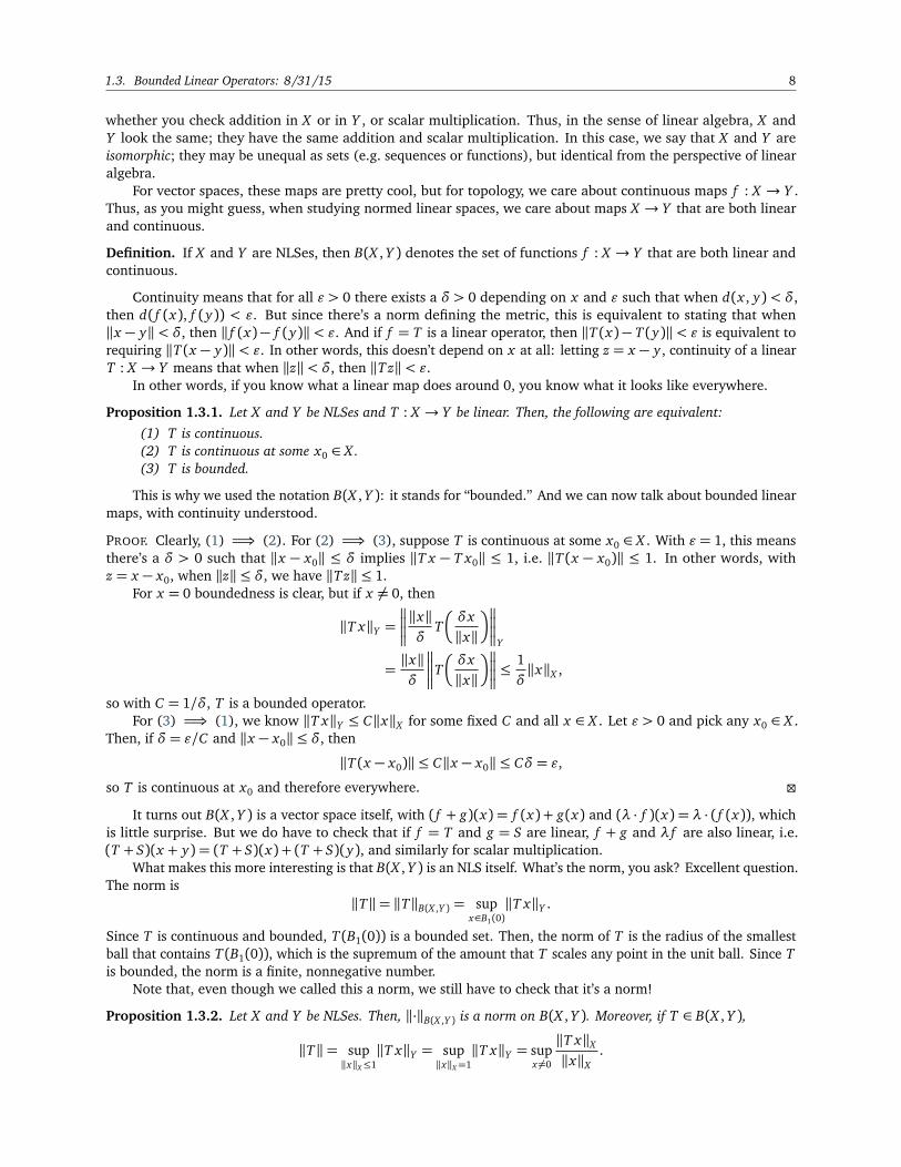
1.3. Bounded Linear Operators: 8/31/15 8
whether you check addition in X or in Y , or scalar multiplication. Thus, in the sense of linear algebra, X andY look the same; they have the same addition and scalar multiplication. In this case, we say that X and Y areisomorphic; they may be unequal as sets (e.g. sequences or functions), but identical from the perspective of linearalgebra.
For vector spaces, these maps are pretty cool, but for topology, we care about continuous maps f : X → Y .Thus, as you might guess, when studying normed linear spaces, we care about maps X → Y that are both linearand continuous.
Definition. If X and Y are NLSes, then B(X , Y ) denotes the set of functions f : X → Y that are both linear andcontinuous.
Continuity means that for all ε > 0 there exists a δ > 0 depending on x and ε such that when d(x , y) < δ,then d( f (x), f (y)) < ε. But since there’s a norm defining the metric, this is equivalent to stating that when‖x − y‖< δ, then ‖ f (x)− f (y)‖< ε. And if f = T is a linear operator, then ‖T (x)− T (y)‖< ε is equivalent torequiring ‖T (x − y)‖< ε. In other words, this doesn’t depend on x at all: letting z = x − y , continuity of a linearT : X → Y means that when ‖z‖< δ, then ‖Tz‖< ε.
In other words, if you know what a linear map does around 0, you know what it looks like everywhere.
Proposition 1.3.1. Let X and Y be NLSes and T : X → Y be linear. Then, the following are equivalent:(1) T is continuous.(2) T is continuous at some x0 ∈ X .(3) T is bounded.
This is why we used the notation B(X , Y ): it stands for “bounded.” And we can now talk about bounded linearmaps, with continuity understood.
PROOF. Clearly, (1) =⇒ (2). For (2) =⇒ (3), suppose T is continuous at some x0 ∈ X . With ε = 1, this meansthere’s a δ > 0 such that ‖x − x0‖ ≤ δ implies ‖T x − T x0‖ ≤ 1, i.e. ‖T(x − x0)‖ ≤ 1. In other words, withz = x − x0, when ‖z‖ ≤ δ, we have ‖Tz‖ ≤ 1.
For x = 0 boundedness is clear, but if x 6= 0, then
‖T x‖Y =
‖x‖δ
T
δx‖x‖
Y
=‖x‖δ
T
δx‖x‖
≤1δ‖x‖X ,
so with C = 1/δ, T is a bounded operator.For (3) =⇒ (1), we know ‖T x‖Y ≤ C‖x‖X for some fixed C and all x ∈ X . Let ε > 0 and pick any x0 ∈ X .
Then, if δ = ε/C and ‖x − x0‖ ≤ δ, then
‖T (x − x0)‖ ≤ C‖x − x0‖ ≤ Cδ = ε,
so T is continuous at x0 and therefore everywhere.
It turns out B(X , Y ) is a vector space itself, with ( f + g)(x) = f (x) + g(x) and (λ · f )(x) = λ · ( f (x)), whichis little surprise. But we do have to check that if f = T and g = S are linear, f + g and λ f are also linear, i.e.(T + S)(x + y) = (T + S)(x) + (T + S)(y), and similarly for scalar multiplication.
What makes this more interesting is that B(X , Y ) is an NLS itself. What’s the norm, you ask? Excellent question.The norm is
‖T‖= ‖T‖B(X ,Y ) = supx∈B1(0)
‖T x‖Y .
Since T is continuous and bounded, T (B1(0)) is a bounded set. Then, the norm of T is the radius of the smallestball that contains T (B1(0)), which is the supremum of the amount that T scales any point in the unit ball. Since Tis bounded, the norm is a finite, nonnegative number.
Note that, even though we called this a norm, we still have to check that it’s a norm!
Proposition 1.3.2. Let X and Y be NLSes. Then, ‖·‖B(X ,Y ) is a norm on B(X , Y ). Moreover, if T ∈ B(X , Y ),
‖T‖= sup‖x‖X≤1
‖T x‖Y = sup‖x‖X=1
‖T x‖Y = supx 6=0
‖T x‖X
‖x‖X.

9 Chapter 1. Normed Linear Spaces and Banach Spaces
Furthermore, if Y is Banach, then B(X , Y ) is too.
This last point is quite interesting: completeness follows when the range is complete, but the domain doesn’tmatter.
PROOF. First, that ‖·‖ is a norm: we have three properties to show.
• We need ‖T‖ = 0 iff T = 0. Clearly, if T = 0 (i.e. T(x) = 0 for all x), then ‖T‖ = supx∈B1(0)‖T x‖ =‖0‖ = 0. Conversely, if we assume ‖T‖ = 0, then for any x ∈ B1(0), ‖T x‖ = 0, so T x = 0. Thus,T |B1(0) = 0. For general x , we’ll scale x = 2‖x‖(x/2‖x‖), so
T x = 2‖x‖T
x2‖x‖
= 2‖x‖ · 0= 0,
since x/2‖x‖ ∈ B1(0). Thus, T = 0.• For linearity of the norm,
‖λT‖= supx∈B1(0)
‖λT x‖= supx∈B1(0)
|λ|‖T x‖= |λ| supx∈B1(0)
‖T x‖= |λ|‖T‖.
Exercise. Finish the proof that this is a norm by addressing the triangle inequality, which isn’t too complicated.
Next, we have the different ways of calculating the norm. The idea is that since T is continuous, the supremumshouldn’t depend on whether the boundary is present or not. One interesting corollary of the formulas forcalculating ‖T‖ is that for any x ∈ X , ‖T x‖ ≤ ‖T‖‖x‖.
The last part does require care. Let Tn∞n=1 be a Cauchy sequence. That is, given an ε > 0, there’s an N > 0such that if m, n ≥ N , then ‖Tn − Tm‖B(X ,Y ) < ε. Thus, given an x ∈ X , ‖Tn x − Tm x‖Y ≤ ‖Tn − Tm‖‖x‖X . Theright-hand side goes to 0 as a Cauchy sequence in m and n, and therefore the left-hand side does too. That is,Tn x∞n−1 ⊂ Y is a Cauchy sequence. Since Y is Banach, this means there’s a limit limn→∞ Tn x = T (x) ∈ Y . Thisdefines a map T : X → Y ; we need to prove that it’s bounded linear and that Tn→ T .
First, let’s look at linearity.
T (x + y) = limn→∞
Tn(x + y) = limn→∞
(Tn x + Tn y).
Since addition is continuous, we can break this up as
= limn→∞
Tn x + limn→∞
Tn y = T x + T y.
Similarly, since scalar multiplication is continuous,
T (λx) = limn→∞
Tn(λx) = λT (x).
Next, let’s check that T is bounded. Since the norm is continuous,
‖T x‖Y =
limn→∞
Tn x
Y
= limn→∞‖Tn x‖Y .
However, this limit a priori might not exist, so we have to use the limsup.
≤ limsupn→∞
‖Tn‖‖x‖X
= M‖x‖X .
Here, M is an upper bound on ‖Tn‖, because Tn is Cauchy and therefore bounded. Thus, we know T ∈ B(X , Y ).Finally, to show Tn→ T , we need to be careful: limits depend on the topology that we’re using, and so we
should be careful that we’re using the topology defined by ‖·‖B(X ,Y ).Let x ∈ B1(0). Then,
‖T x − T y‖Y = limm→∞
‖Tm x − Tn x‖
= limm→∞
‖(Tm − Tn)x‖
≤ lim supm→∞
‖Tm − Tn‖‖x‖.
Since Tn is Cauchy, then for any ε > 0, ‖Tm − Tn‖< ε when m, n are sufficiently large, and therefore the limsupgoes to 0 as n→∞, and so Tn→ T .
1.4. `p-norms: 9/2/15 10
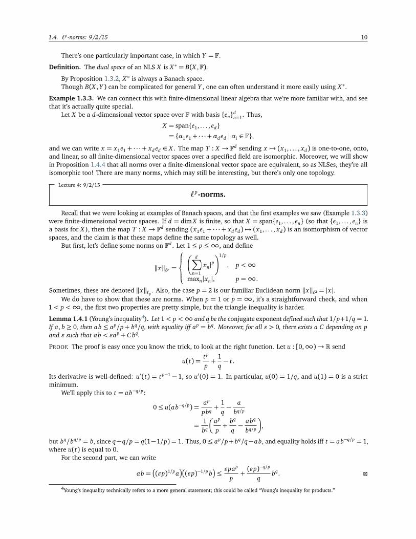
There’s one particularly important case, in which Y = F.
Definition. The dual space of an NLS X is X ∗ = B(X ,F).
By Proposition 1.3.2, X ∗ is always a Banach space.Though B(X , Y ) can be complicated for general Y , one can often understand it more easily using X ∗.
Example 1.3.3. We can connect this with finite-dimensional linear algebra that we’re more familiar with, and seethat it’s actually quite special.
Let X be a d-dimensional vector space over F with basis endn=1. Thus,
X = spane1, . . . , ed= α1e1 + · · ·+αd ed | αi ∈ F,
and we can write x = x1e1 + · · ·+ xd ed ∈ X . The map T : X → Fd sending x 7→ (x1, . . . , xd) is one-to-one, onto,and linear, so all finite-dimensional vector spaces over a specified field are isomorphic. Moreover, we will showin Proposition 1.4.4 that all norms over a finite-dimensional vector space are equivalent, so as NLSes, they’re allisomorphic too! There are many norms, which may still be interesting, but there’s only one topology.
Lecture 4: 9/2/15
`p-norms.
Recall that we were looking at examples of Banach spaces, and that the first examples we saw (Example 1.3.3)were finite-dimensional vector spaces. If d = dim X is finite, so that X = spane1, . . . , en (so that e1, . . . , en isa basis for X ), then the map T : X → Fd sending (x1e1 + · · ·+ xd ed) 7→ (x1, . . . , xd) is an isomorphism of vectorspaces, and the claim is that these maps define the same topology as well.
But first, let’s define some norms on Fd . Let 1≤ p ≤∞, and define
‖x‖`p =
d∑
n=1
|xn|p
1/p
, p <∞
maxn|xn|, p =∞.
Sometimes, these are denoted ‖x‖`p. Also, the case p = 2 is our familiar Euclidean norm ‖x‖`2 = |x |.
We do have to show that these are norms. When p = 1 or p =∞, it’s a straightforward check, and when1< p <∞, the first two properties are pretty simple, but the triangle inequality is harder.
Lemma 1.4.1 (Young’s inequality4). Let 1< p <∞ and q be the conjugate exponent defined such that 1/p+1/q = 1.If a, b ≥ 0, then ab ≤ ap/p+ bq/q, with equality iff ap = bq. Moreover, for all ε > 0, there exists a C depending on pand ε such that ab < εap + C bq.
PROOF. The proof is easy once you know the trick, to look at the right function. Let u : [0,∞)→ R send
u(t) =t p
p+
1q− t.
Its derivative is well-defined: u′(t) = t p−1 − 1, so u′(0) = 1. In particular, u(0) = 1/q, and u(1) = 0 is a strictminimum.
We’ll apply this to t = ab−q/p:
0≤ u(ab−q/p) =ap
pbq+
1q−
abq/p
=1bq
ap
p+
bq
q−
abq
bq/p
,
but bq/bq/p = b, since q−q/p = q(1−1/p) = 1. Thus, 0≤ ap/p+ bq/q−ab, and equality holds iff t = ab−q/p = 1,where u(t) is equal to 0.
For the second part, we can write
ab =
(εp)1/pa
(εp)−1/p b
≤εpap
p+(εp)−q/p
qbq.
4Young’s inequality technically refers to a more general statement; this could be called “Young’s inequality for products.”

11 Chapter 1. Normed Linear Spaces and Banach Spaces
For conjugate exponents, we have the convention that the conjugate of 1 is∞, and vice versa.
Theorem 1.4.2 (Hölder’s inequality). Let 1≤ p ≤∞ and q be its conjugate exponent. If x , y ∈ Fd , then∑
n
|xn yn| ≤ ‖x‖`p‖y‖`q .
When p = 2, this is also known as the Cauchy-Schwarz inequality.
PROOF. The cases p = 1,∞ are trivial; expand their definitions out. Similarly, if x = 0 or y = 0, there’s not a lotto say. Thus, we’re left with 1< p <∞, so we can use Lemma 1.4.1.
Let a = |xn|/‖x‖`p and b = |yn|/‖y‖`q . Then, by Lemma 1.4.1,
|xn|‖x‖`p
|yn|‖y‖`q
≤|xn|
p
p‖x‖p`p
+|yn|
q
q‖y‖q`q
,
so summing all n of those,∑
n|xn yn|‖x‖`p‖y‖`q
≤∑
|xn|p
p‖x‖p`p
+
∑
|yn|q
q‖y‖q`q
=‖x‖p
`p
p‖x‖p`p
+‖y‖q
`q
q‖x‖q`q
=1p+
1q= 1.
Now, we can use this to prove the triangle inequality for ‖·‖`p . We’ll need two things for the Hölder inequality,so just take one term out of the pth power:
‖x + y‖p`p =
d∑
n=1
|xn + yn|p
≤d∑
n=1
|xn + yn|p−1(|xn|+ |yn|)
≤
d∑
n=1
|xn + yn|(p−1)q
1/q
(‖x‖`p + ‖y‖`q).
Since p and q are conjugate, p = (p− 1)q, so the first term is ‖x − y‖p/q`p . Thus,
‖x + y‖p−p/q`p ≤ ‖x‖`p + ‖y‖`p ,
and p− p/q = 1, so we’re done.Moreover, all these norms are equivalent.
Proposition 1.4.3. Let 1≤ p ≤∞. Then, for all x ∈ Fd ,
‖x‖`∞ ≤ ‖x‖`p ≤ d1/p‖x‖`∞ .
These estimates are sharp, the first at x = (1, 0,0 . . . , 0), and the second at x = (1, 1, . . . , 1).
PROOF. Let m be an index for which |xm|=maxn|xn|. Since f (x) = x1/p is an increasing function,
‖x‖`∞ = |xm|= (|xm|p)1/p ≤
d∑
n=1
|xn|p
1/p
= ‖x‖`p ,

1.5. `p and Lp-spaces: 9/4/15 12
and
‖x‖`p =
d∑
n=1
|xn|p
1/p
≤
d∑
1
|xm|p
1/p
= (d|xm|p)1/p = d1/p‖x‖`∞ .
Notice that some of these proof methods fail horribly in infinite dimensions.It turns out that on all finite-dimensional vector spaces, all norms are equivalent.
Proposition 1.4.4. All norms on a finite-dimensional NLS are equivalent. Moreover, a K ⊂ X is compact iff it is closedand bounded.
That means there’s only one topology.
PROOF. Let d = dim X and endn=1 be a basis. Then, let T : X → Fd be the coordinate map defined above. Let ∼=denote an isomorphism of NLSes.
We’ll define a norm ‖·‖1 on x by ‖x‖1 = ‖T x‖`1 : of the three properties, the last two are trivial (since T islinear), so we just need to prove that ‖x‖1 = 0 iff x = 0. But T is one-to-one and onto, so this follows, and ‖·‖1 isin fact a norm.5
Thus, (X ,‖·‖1) ∼= (Fd ,‖·‖`1), so they really are the “same” space. This is because T : X → Fd is a boundedmap, with C = 1, and therefore continuous, and T−1 is also linear and continuous. Thus, T is an isomorphism ofvector spaces and a homeomorphism of topological spaces, so we can take results in Fd and apply them to X .
The Heine-Borel theorem from undergraduate real analysis tells us that K ⊂ Fd is closed and boundediff it’s compact. But since X and Fd have the same topology, then this is also true in X . In particular, S1
1 =x ∈ X : ‖x‖1 = 1 is also compact.
Now, for any norm ‖·‖ on X and x ∈ X ,
‖x‖=
d∑
n=1
xnen
≤d∑
n=1
|xn|‖en‖ ≤ C‖x‖1,
where C = maxn‖en‖. Notice that this step won’t work in infinite dimensions. Our upper bound implies that(Top)‖·‖ ⊆ (Top)‖·‖1
, so the former topology is said to be stronger. We’ll prove the two are equal by providing alower bound.
We have a continuous map ‖·‖ : (X ,‖·‖1) → R. It’s also continuous as a map ‖·‖ : (X ,‖·‖) → R. Leta = infx∈S1
1‖x‖; since S1 is compact and the norm is continuous, the minimum is attained, and it must be positive
(because 0 6∈ S11).
Thus, for any x ∈ X , ‖x/‖x‖1‖ ≥ a, so ‖x‖ ≥ a‖x‖1, which is our desired lower bound.
Corollary 1.4.5. If X is a d-dimensional NLS, then X ∼= Fd .
Corollary 1.4.6. If X and Y are NLSes and X is finite-dimensional, then every linear T : X → Y is bounded andX ∗ = Fd , given by T (x) = y · x.
Lecture 5: 9/4/15
`p and Lp-spaces.
“There are different sizes of infinity, and this one is the best.”
Last time we showed that if (X ,‖·‖) is a finite-dimensional NLS, then it’s isomorphic and homeomorphic to(Fd ,‖·‖`2), where d = dim X . Moreover, X is Banach, and (Fd)∗ ∼= Fd . Finite dimensions aren’t very interesting,but they’re a good place to gain intuition.
A lot of this nice stuff goes away for infinite-dimensional spaces, and some are nicer than others.
5A great way to create a new norm is to map from one space to another (or the same one) and pull the norm back.

13 Chapter 1. Normed Linear Spaces and Banach Spaces
Example 1.5.1. Let 1≤ p ≤∞. We’ll define a space `p which behaves sort of like an “F∞.” Specifically,
`p =
x = xn∞n=1 : xn ∈ F,‖x‖`p <∞
,
where
‖x‖`p =
∞∑
n=1
|xn|p
1/p
, p finite
supn|xn|, p =∞.The same proofs for the `p-norms in finite-dimensional spaces apply, and show that `p is an NLS.
Theorem 1.5.2 (Hölder’s inequality in `p). If 1≤ p ≤∞, 1/p+ 1/q = 1, and x ∈ `p and y ∈ `q, then∞∑
n=1
|xn yn| ≤ ‖x‖`p‖y‖`q .
Again, the proof is identical to the one for the finite-dimensional `p-norm.Note that `∞ can be a bit weird relative to the rest of the `p spaces.If p is finite, then `p has countably infinite dimension, i.e. it has a basis that’s countable. This is subtle: the span
of a basis is the set of finite linear combinations; in the infinite case, we would have to worry about convergence.Anyways, set
ein =§
1, i = n0, i 6= n.
Then, a basis for `p, called the Schauder basis, isB = ei∞i=1, and its span is
span(B) =¦
αi1 ei1 +αi2 ei2 + · · ·+αin ein : n ∈ N,αi j∈ F
©
.
Note that this is not a basis in the linear-algebraic sense (which would have to be uncountable); rather, this meansthat `p is the closure of span(B). That is, for all x ∈ `p, there’s a unique representation x =
∑∞j=1 x je
j , meaningthat if xN denotes the N th partial sum, then xN ∈ span(B) for all N , and
‖x − xN‖`p =
∞∑
n=N+1
|xn|p
1/p
−→ 0.
This is a little weird, but the point is that, since you can’t take infinite sums in a basis, things can get a little strange.But everything comes from the finite case.
`∞ does not have a countable basis. As a result, we sometimes consider subspaces with a countable basis.Define
c0 = x ∈ `∞ : limn→∞
xn = 0 and
f0 = x ∈ `∞ : xn = 0 for all but finitely many n.
For example, (1, 1, 1 . . . ) ∈ `∞, but it’s not in c0 or f0, and (1, 1/2, 1/3, . . . ) is in c0 but not f0. f0 and c0 inherit the`∞-norm and become NLSes in their own right.
If 1≤ p ≤ q <∞, then we have the following chain of inclusions:
f0 ( `p ⊆ `q ( c0 ( `∞.
If you’re looking for examples (or, sometimes, counterexamples), c0 and f0 are often useful. For example, onf0, we have a function T : f0→ F defined by
T (x) =∞∑
n=1
nxn.
Since each α ∈ f0 is a finite sequence, then this is well-defined, and it’s linear, but it’s not bounded, since T (ei) = ibut ‖ei‖`∞ = 1 for all i. Thus, we have a linear map which is not continuous.
Exercise. If 1≤ p ≤∞, show that `p is Banach.
This is conceptually easy but a bit of work, coming down to calculus, and so we know that limits of Cauchysequences exist. However, since `1 is a subspace of `∞, we can consider the NLS (`1,‖·‖`∞); this space is notBanach.
1.5. `p and Lp-spaces: 9/4/15 14
Lemma 1.5.3. Let 0< p < 1 and define `p in the same way as above. In this case, however, `p is not an NLS, because‖·‖`p isn’t a norm.
PROOF IDEA. We can look at (F2,‖·‖`p) to see this: we proved that, given the triangle inequality, the unit ball isconvex. However, the unit ball isn’t convex when p < 1. The same proof works for `p, but with a less explicitpicture.
The Hölder inequality allows us to create many continuous linear functionals T : `p → F when 1≤ p ≤∞.Let q be the conjugate exponent (so 1/p+ 1/q = 1), and choose any y ∈ `q. Then, we can produce a Ty ∈ (`p)∗,i.e. Ty : `p → F, defined by
Ty(x) =∞∑
n=1
xn yn.
Moreover, Ty is bounded, because |Ty(x)| ≤ ‖y‖`q‖x‖`p .This defines an inclusion `q ,→ (`p)∗.
Exercise. In fact, when p is finite, `q = (`p)∗. Moreover, T : `q → (`p)∗ sending T (y)→ Ty is a bounded operator,as ‖Ty‖(`p)∗ = ‖y‖`q .
That is, the dual space is the conjugate space; to show this, figure out how to write T(ei) as yi for someyi ∈ `q.
The above result is untrue for `∞; in fact, (`∞)∗ ) `1, but c∗0 = `1.
That’s all that we really need to say about `p for now; it’s one step up from finite-dimensional spaces, and is abit different, but not all that exotic. Right now, our examples are Fd , which is finite-dimensional; `p when p isfinite, which has a countable basis, and `∞, which has no countable basis.
Lesbegue spaces. Let Ω ⊆ Rd be a measurable set with nonzero measure. We want to define a space offunctions on Ω. However, when we talk about functions and measure, we really want to define two functions fand g as “the same” if f (x) = g(x) except on a set of measure zero. If this is true, no integral can distinguish fand g.
FIGURE 1.1. An example of an LP space. Source: http://iloveaustin.tumblr.com/.

15 Chapter 1. Normed Linear Spaces and Banach Spaces
Definition. Let 1≤ p <∞, and define Lp(Ω) be the set of measurable functions6 f : Ω→ F such that∫
Ω| f (x)|p dx
is finite. Lp(Ω) becomes an NLS with the norm
‖ f ‖p =
∫
Ω
| f (x)|p1/p
,
though we’ll have to show that.
Once again, we can define this for p < 1, but it won’t end up being a norm.When p =∞, we’ll do things a little differently, as usual.
Definition.• A measurable f : Ω→ F is essentially bounded by K ∈ R if | f (x)| ≤ K for almost every x ∈ Ω (i.e. the set
where this is not true has measure zero).• The essential supremum of f , denoted ess supx∈Ω| f (x)|, is the infimum of the K that essentially bound f .
Then, we can define L∞(Ω) as the set of (equivalence classes of) measurable functions whose essentialsuprema are finite, and ‖ f ‖∞ = ess supx∈Ω| f (x)|. This will also be an NLS, though we’ll have to show that too.
Proposition 1.5.4. If 0< p ≤∞, then Lp(Ω) is a vector space, and ‖ f ‖p = 0 iff f = 0 almost everywhere on Ω.
PROOF. First, why is Lp(Ω) closed under addition? If p is finite, then
| f (x) + g(x)|p ≤ (| f (x)|+ |g(x)|)p ≤ 2p(| f (x)|p + |g(x)|p),
so when one integrates, if f , g ∈ Lp(Ω), then the rightmost quantity is bounded and therefore the leftmost one is.Scalar multiplication (and the scaling property of the norm) is easy: just write down the definition.
For p = ∞, the maximum of the sum cannot be bigger than the sum of the maxima, so ‖ f + g‖∞ =‖ f ‖∞ + ‖g‖∞. Scaling and scalar multiplication are also straightforward.
Thus, all we have left is the triangle inequality, which we’ll show next class.
Lecture 6: 9/9/15
Lp(Ω) is Banach.
Recall that if Ω ⊆ Rd , then Lp(Ω) is the set of equivalence classes of measurable functions Ω → F with‖ f ‖p <∞, where f ∼ g if they differ on a set of measure zero. Then, the p-norm is
‖ f ‖p =
∫
Ω
| f (x)|p dx
1/p
, p <∞
ess supx∈Ω| f (x)|, p =∞.
Last time, we showed that Lp(Ω) is a vector space, and two of the properties of NLSes, the zero and scalingproperties. Today we’ll attack the triangle inequality; just as for `p, we’ll need Hölder’s inequality.
Proposition 1.6.1 (Hölder’s inequality for Lp). Let 1 ≤ p ≤∞ and 1/p+ 1/q = 1. If f ∈ Lp(Ω) and g ∈ Lq(Ω),then f g ∈ L1(Ω) and ‖ f g‖1 ≤ ‖ f ‖p‖g‖q, with equality iff | f (x)|p is proportional to |g(x)|q.
PROOF. If p = 1 or p =∞, we already know that∫
Ω| f (x)g(x)|dx ≤ ‖g‖∞
∫
Ω| f |dx = ‖ f ‖1‖g‖∞.
If 1< p <∞, we know from Lemma 1.4.1 that ab ≤ ap/p+ bq/q, with equality when ap = bq. If ‖ f ‖p = 0or ‖g‖q = 0, then we’re done; otherwise,
| f (x)|‖ f ‖p
|g(x)|‖g‖q
≤| f (x)|p
‖ f ‖pp p+|g(x)|q
‖g‖qqq
,
so integrating, we get∫
| f g|‖ f ‖p‖g‖q
≤ 1,
with equality when | f (x)|p/‖ f ‖pp = |g(x)|
q/‖g‖qq, which gives us our proportionality.
6To be pedantic, the elements of Lp(Ω) are equivalence classes of functions that differ from f on a set of measure zero, since the integralsare the same.

1.6. Lp(Ω) is Banach: 9/9/15 16
Theorem 1.6.2 (Minkowski’s inequality). If 1≤ p ≤∞, then ‖ f + g‖p ≤ ‖ f ‖p + ‖g‖p.
PROOF. Notice that if f or g isn’t in Lp(Ω), then its p-norm is infinite, so we’re done. The result is also clear ifp = 1 or p =∞: the supremum of the sum is less than the sum of the suprema, and similarly with absolute value.
So we only have to worry about 1 < p <∞, and here we’ll use a similar trick as for `p spaces, taking onecopy of a pth power.
‖ f + g‖pp =
∫
Ω
| f (x) + g(x)|p dx
≤∫
Ω
| f (x) + g(x)|p−1(| f (x)|+ |g(x)|)dx .
Using Hölder’s inequality,
≤∫
Ω
| f (x) + g(x)|(p−1)q
1/q
‖ f ‖p + ‖g‖p
= ‖ f + g‖p−1p
‖ f ‖p + ‖g‖p
,
so dividing by ‖ f + g‖p−1, we’re done.
Lp spaces are very important in analysis, and form an important set of examples for NLSes. A little later, we’llshow that they’re complete, but we should note that we’re measuring the size of a function using varying p, whichmeasure different things, between emphasizing large values at a point, or large values at infinity.
On R, imagine a function that goes to∞ as x → 0+ and 0 as x →∞. If p is large, we’re emphasizing thelarge values of the function, so if it grows too quickly it might not be in Lp(R). If p is small, then we’re emphasizingthe long tail as x →∞; if it dies too slowly, it might not be in Lp(R). An instructive example is x p, which is insome Lq spaces but not others.
An easier way to think about this is to bound Ω, so we don’t have to worry about long tails.
Proposition 1.6.3. Let µ denote the Lesbegue measure, and suppose µ(Ω) is finite. Let 1≤ p ≤ q ≤∞.(1) If f ∈ Lq(Ω), then f ∈ Lp(Ω), and in fact ‖ f ‖p = (µ(Ω))1/p−1/q‖ f ‖q.(2) If f ∈ L∞(Ω), then f ∈ Lp(Ω) for 1≤ p ≤<∞, and limp→∞‖ f ‖p = ‖ f ‖∞.(3) If f ∈ Lp(Ω) for 1≤ p <∞ and ‖ f ‖p ≤ K for all such p, then f ∈ L∞(Ω) and ‖ f ‖∞ ≤ K.
These will be proven in the homework. Part (2) is the reason the L∞-norm is named such. Note also thatthere exist f such that f ∈ Lp(Ω) for 1≤ p <∞ but f 6∈ L∞(Ω), even when Ω has finite measure.
The general proof idea is to consider sets of bad points and see what happens.
Proposition 1.6.4. For 1≤ p ≤∞ and Ω measurable, Lp(Ω) is complete.
Thus, we have another useful class of Banach spaces.
PROOF. As usual, we’ll start with a Cauchy sequence fn(x)∞n=1 in Lp(Ω). The idea will be to write
fn(x) = f1(x) + f2(x)− f1(x) + f3(x)− f2(x) + · · ·+ fn(x)− fn−1(x),
so if we group the fi(x)− fi−1(x), then these pieces should be small, and therefore we ought to converge to somefunction f (x). There are technical problems, though, since we don’t know how fast the fn converge, so we need totry fi(x)− fi−k(x) for k > 1. Moreover, we’ll use absolute values. This is the idea; now, let’s write it down carefully.
First, select a subsequence such that ‖ fn j+1− fn j
‖ ≤ 2− j for all j; we can do this because if we have n j−1, there’san n j such that ‖ fn j
− fm‖ ≤ 2− j when m≥ n j ≥ n j−1.Let
Fm(x) = | fn1(x)|+
m∑
j=1
| fn j+1(x)− fn j
(x)| ≥ 0,
so that Fm(x) is increasing in m pointwise, so there’s a limit (which might be∞, but that’s OK). Let F(x) =limm→∞ Fm(x) ∈ [0,∞]. Then,
‖Fm‖p ≤ ‖ fn1‖p +
n∑
j=1
2− j ≤ ‖ fn1‖p + 1,
which is finite. But more interestingly, F ∈ Lp(Ω) too! We’ll have to treat L∞ as a special case again.
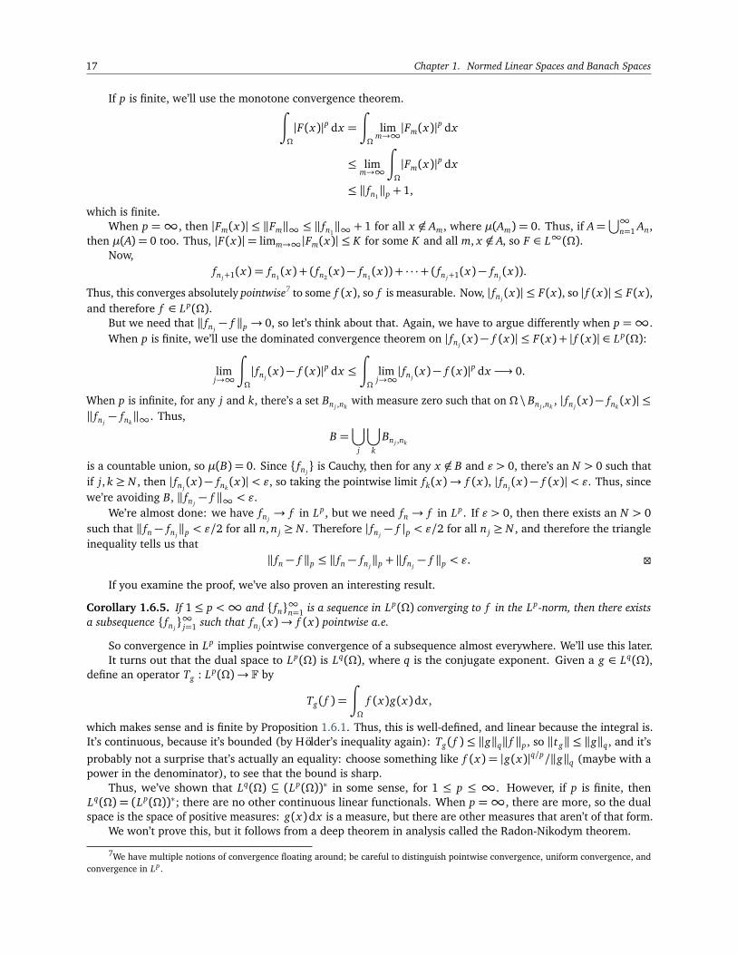
17 Chapter 1. Normed Linear Spaces and Banach Spaces
If p is finite, we’ll use the monotone convergence theorem.∫
Ω
|F(x)|p dx =
∫
Ω
limm→∞
|Fm(x)|p dx
≤ limm→∞
∫
Ω
|Fm(x)|p dx
≤ ‖ fn1‖p + 1,
which is finite.When p =∞, then |Fm(x)| ≤ ‖Fm‖∞ ≤ ‖ fn1
‖∞ + 1 for all x 6∈ Am, where µ(Am) = 0. Thus, if A=⋃∞
n=1 An,then µ(A) = 0 too. Thus, |F(x)|= limm→∞|Fm(x)| ≤ K for some K and all m, x 6∈ A, so F ∈ L∞(Ω).
Now,fn j+1(x) = fn1
(x) + ( fn2(x)− fn1
(x)) + · · ·+ ( fn j+1(x)− fn j(x)).
Thus, this converges absolutely pointwise7 to some f (x), so f is measurable. Now, | fn j(x)| ≤ F(x), so | f (x)| ≤ F(x),
and therefore f ∈ Lp(Ω).But we need that ‖ fn j
− f ‖p → 0, so let’s think about that. Again, we have to argue differently when p =∞.When p is finite, we’ll use the dominated convergence theorem on | fn j
(x)− f (x)| ≤ F(x) + | f (x)| ∈ Lp(Ω):
limj→∞
∫
Ω
| fn j(x)− f (x)|p dx ≤
∫
Ω
limj→∞| fn j(x)− f (x)|p dx −→ 0.
When p is infinite, for any j and k, there’s a set Bn j ,nkwith measure zero such that on Ω \ Bn j ,nk
, | fn j(x)− fnk
(x)| ≤‖ fn j− fnk
‖∞. Thus,
B =⋃
j
⋃
k
Bn j ,nk
is a countable union, so µ(B) = 0. Since fn j is Cauchy, then for any x 6∈ B and ε > 0, there’s an N > 0 such that
if j, k ≥ N , then | fn j(x)− fnk
(x)|< ε, so taking the pointwise limit fk(x)→ f (x), | fn j(x)− f (x)|< ε. Thus, since
we’re avoiding B, ‖ fn j− f ‖∞ < ε.
We’re almost done: we have fn j→ f in Lp, but we need fn → f in Lp. If ε > 0, then there exists an N > 0
such that ‖ fn − fn j‖p < ε/2 for all n, n j ≥ N . Therefore | fn j
− f |p < ε/2 for all n j ≥ N , and therefore the triangleinequality tells us that
‖ fn − f ‖p ≤ ‖ fn − fn j‖p + ‖ fn j
− f ‖p < ε.
If you examine the proof, we’ve also proven an interesting result.
Corollary 1.6.5. If 1≤ p <∞ and fn∞n=1 is a sequence in Lp(Ω) converging to f in the Lp-norm, then there existsa subsequence fn j
∞j=1 such that fn j(x)→ f (x) pointwise a.e.
So convergence in Lp implies pointwise convergence of a subsequence almost everywhere. We’ll use this later.It turns out that the dual space to Lp(Ω) is Lq(Ω), where q is the conjugate exponent. Given a g ∈ Lq(Ω),
define an operator Tg : Lp(Ω)→ F by
Tg( f ) =
∫
Ω
f (x)g(x)dx ,
which makes sense and is finite by Proposition 1.6.1. Thus, this is well-defined, and linear because the integral is.It’s continuous, because it’s bounded (by Hölder’s inequality again): Tg( f )≤ ‖g‖q‖ f ‖p, so ‖t g‖ ≤ ‖g‖q, and it’sprobably not a surprise that’s actually an equality: choose something like f (x) = |g(x)|q/p/‖g‖q (maybe with apower in the denominator), to see that the bound is sharp.
Thus, we’ve shown that Lq(Ω) ⊆ (Lp(Ω))∗ in some sense, for 1 ≤ p ≤ ∞. However, if p is finite, thenLq(Ω) = (Lp(Ω))∗; there are no other continuous linear functionals. When p =∞, there are more, so the dualspace is the space of positive measures: g(x)dx is a measure, but there are other measures that aren’t of that form.
We won’t prove this, but it follows from a deep theorem in analysis called the Radon-Nikodym theorem.
7We have multiple notions of convergence floating around; be careful to distinguish pointwise convergence, uniform convergence, andconvergence in Lp .

1.7. The Hahn-Banach Theorem: 9/11/15 18
Lecture 7: 9/11/15
The Hahn-Banach Theorem.
“Almost everything has three properties. Have you noticed that?”
Corollary 1.7.1. Let X be an NLS, Y ⊂ X be a linear subspace, and f : Y → F be bounded. Then, there exists anF ∈ X ∗ such that F |Y = f and ‖F‖X ∗ = ‖ f ‖Y ∗ .
Though Lp functions can be complicated, all of them can be well-approximated by less complicated functions.Recall that a simple function is a Lesbegue-integrable function that takes on only finitely many values, and that afunction is compactly supported if it is equal to 0 outside of a compact set.
Proposition 1.7.2. For 1≤ p ≤∞, the set S of all measurable simple functions with compact support is dense inLp(Ω).
This says that for any f ∈ Lp(Ω) and ε > 0, there’s a ϕ ∈ S such that ‖ f −ϕ‖Lp(Ω) < ε. The proof comes frommeasure theory: the integral was defined by the limit of approximations by simple functions, and so these simplefunctions are successively better approximations.
Definition. Let C∞0 (Ω) denote the space of compactly supported, continuous functions.
Proposition 1.7.3. If Ω is an open set and 1≤ p <∞, then C∞0 (Ω) is dense in Lp(Ω).
The proof follows from another measure-theoretic result called Lusin’s theorem.Now, we’ll move into some deeper (and, well, harder) theorems and questions in functional analysis. We’ll
start with a question.Let X be a finite-dimensional NLS and Y ⊂ X be a subspace. Given a linear f : Y → R, can we extend f to X ?
The answer is yes. But what about the infinite-dimensional case? Here, we care about continuous (so bounded)linear operators.
Once again, the answer is that it’s possible, but this is hard to prove, and it’ll take us a while to prove that. Wewon’t need all the properties of a norm to prove that, so we can weaken what we need in terms of the norm.
Definition. Let X be a vector space over F. We say that p : X → [0,∞) is sublinear if
(1) p(λx) = λp(x) for all λ≥ 0 and x ∈ X , and(2) p(x + y)≤ p(x) + p(y) for all x , y ∈ X .
If in addition p satisfies (1) for all λ ∈ F, p is called a seminorm.
If a seminorm also satisfies p(x) = 0 implies x = 0, then p is a norm.The Hahn-Banach theorem about extension of linear operators will apply perfectly well to sublinear operators.
First, let’s deal with the simplest version we can think of.
Lemma 1.7.4. Let X be a vector space over R and Y ( X be a linear subspace. Let p be sublinear on X and f : Y → Rbe linear such that f (y)≤ p(y) for all y ∈ Y . For a given x0 ∈ X \ Y , let eY = spanY, x0= Y +Rx0 = y +λx0 :y ∈ Y,λ ∈ R; then, there exists a linear map ef : eY → R such that ef |Y = f and −p(−x)≤ ef (x)≤ p(x) for all x ∈ eY .
The definitions of eY all show that it’s “Y plus one more dimension.”
PROOF. If ef (x)≤ p(x), then −ef (x) = ef (−x)≤ p(−x), so ef (x)≥ −p(−x), and so the lower bound comes for free.We’ll present the proof not as a cleaned-up proof, but how one would think of the proof when trying to prove
it.If we had such an ef , what would it look like? ey ∈ eY can be written ey = y +λx0 for some y ∈ Y and λ ∈ R,
so ef (ey) = ef (y +λx0) = ef (y) +λef (x0) = f (y) +λef (x0), since ef |Y = f .So if we had defined α ∈ R to be ef (x0), then we get a function, and correspondingly, given ef , we get α = ef (x0).
Thus, ef is characterized by α.However, we need to be careful: is this really well-defined? We chose y; what if you choose a different one
than I do? It turns out that you have to choose the same y: suppose ey = y + λx0 = z + µx0 for y, z ∈ Y andλ,µ ∈ R. Thus, y − z = (µ−λ)x0, but y − z ∈ Y , so since x0 6∈ Y , then µ−λ= 0, and therefore y = z; thus, thischoice of y is well-defined, so ef really is characterized by α.
19 Chapter 1. Normed Linear Spaces and Banach Spaces
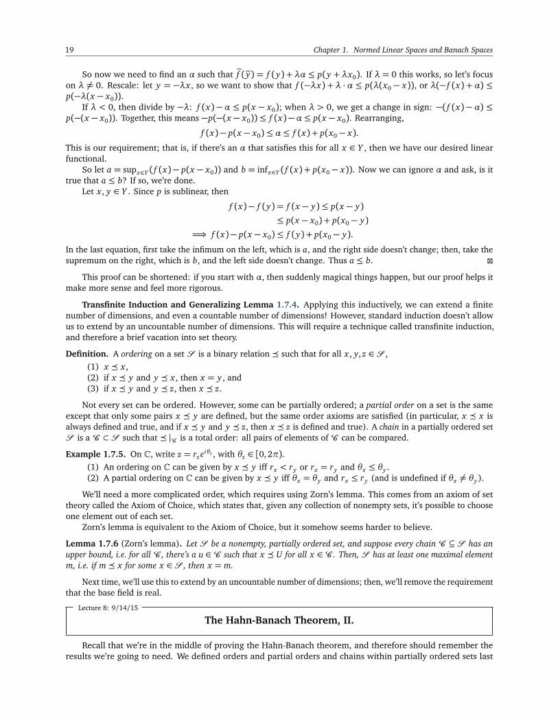
So now we need to find an α such that ef (ey) = f (y) + λα ≤ p(y + λx0). If λ = 0 this works, so let’s focuson λ 6= 0. Rescale: let y = −λx , so we want to show that f (−λx) + λ · α ≤ p(λ(x0 − x)), or λ(− f (x) + α) ≤p(−λ(x − x0)).
If λ < 0, then divide by −λ: f (x)− α ≤ p(x − x0); when λ > 0, we get a change in sign: −( f (x)− α) ≤p(−(x − x0)). Together, this means −p(−(x − x0))≤ f (x)−α≤ p(x − x0). Rearranging,
f (x)− p(x − x0)≤ α≤ f (x) + p(x0 − x).
This is our requirement; that is, if there’s an α that satisfies this for all x ∈ Y , then we have our desired linearfunctional.
So let a = supx∈Y ( f (x)− p(x − x0)) and b = infx∈Y ( f (x) + p(x0 − x)). Now we can ignore α and ask, is ittrue that a ≤ b? If so, we’re done.
Let x , y ∈ Y . Since p is sublinear, then
f (x)− f (y) = f (x − y)≤ p(x − y)
≤ p(x − x0) + p(x0 − y)
=⇒ f (x)− p(x − x0)≤ f (y) + p(x0 − y).
In the last equation, first take the infimum on the left, which is a, and the right side doesn’t change; then, take thesupremum on the right, which is b, and the left side doesn’t change. Thus a ≤ b.
This proof can be shortened: if you start with α, then suddenly magical things happen, but our proof helps itmake more sense and feel more rigorous.
Transfinite Induction and Generalizing Lemma 1.7.4. Applying this inductively, we can extend a finitenumber of dimensions, and even a countable number of dimensions! However, standard induction doesn’t allowus to extend by an uncountable number of dimensions. This will require a technique called transfinite induction,and therefore a brief vacation into set theory.
Definition. A ordering on a set S is a binary relation such that for all x , y, z ∈ S ,(1) x x ,(2) if x y and y x , then x = y , and(3) if x y and y z, then x z.
Not every set can be ordered. However, some can be partially ordered; a partial order on a set is the sameexcept that only some pairs x y are defined, but the same order axioms are satisfied (in particular, x x isalways defined and true, and if x y and y z, then x z is defined and true). A chain in a partially ordered setS is a C ⊂ S such that |C is a total order: all pairs of elements of C can be compared.
Example 1.7.5. On C, write z = rzeiθz , with θz ∈ [0,2π).(1) An ordering on C can be given by x y iff rx < ry or rx = ry and θx ≤ θy .(2) A partial ordering on C can be given by x y iff θx = θy and rx ≤ ry (and is undefined if θx 6= θy).
We’ll need a more complicated order, which requires using Zorn’s lemma. This comes from an axiom of settheory called the Axiom of Choice, which states that, given any collection of nonempty sets, it’s possible to chooseone element out of each set.
Zorn’s lemma is equivalent to the Axiom of Choice, but it somehow seems harder to believe.
Lemma 1.7.6 (Zorn’s lemma). Let S be a nonempty, partially ordered set, and suppose every chain C ⊆ S has anupper bound, i.e. for all C , there’s a u ∈ C such that x U for all x ∈ C . Then, S has at least one maximal elementm, i.e. if m x for some x ∈ S , then x = m.
Next time, we’ll use this to extend by an uncountable number of dimensions; then, we’ll remove the requirementthat the base field is real.
Lecture 8: 9/14/15
The Hahn-Banach Theorem, II.
Recall that we’re in the middle of proving the Hahn-Banach theorem, and therefore should remember theresults we’re going to need. We defined orders and partial orders and chains within partially ordered sets last
1.8. The Hahn-Banach Theorem, II: 9/14/15 20
lecture, and cited Zorn’s lemma, Lemma 1.7.6, which gives conditions for when a partially ordered set has amaximal element. Finally, we have Corollary 1.7.1 in mind as a long-term goal.
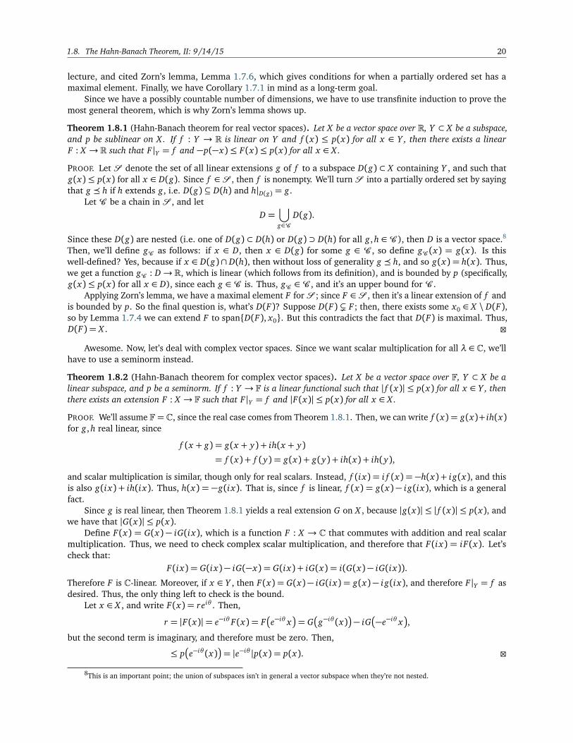
Since we have a possibly countable number of dimensions, we have to use transfinite induction to prove themost general theorem, which is why Zorn’s lemma shows up.
Theorem 1.8.1 (Hahn-Banach theorem for real vector spaces). Let X be a vector space over R, Y ⊂ X be a subspace,and p be sublinear on X . If f : Y → R is linear on Y and f (x) ≤ p(x) for all x ∈ Y , then there exists a linearF : X → R such that F |Y = f and −p(−x)≤ F(x)≤ p(x) for all x ∈ X .
PROOF. Let S denote the set of all linear extensions g of f to a subspace D(g) ⊂ X containing Y , and such thatg(x)≤ p(x) for all x ∈ D(g). Since f ∈ S , then f is nonempty. We’ll turn S into a partially ordered set by sayingthat g h if h extends g, i.e. D(g) ⊆ D(h) and h|D(g) = g.
Let C be a chain in S , and letD =
⋃
g∈CD(g).
Since these D(g) are nested (i.e. one of D(g) ⊂ D(h) or D(g) ⊃ D(h) for all g, h ∈ C ), then D is a vector space.8
Then, we’ll define gC as follows: if x ∈ D, then x ∈ D(g) for some g ∈ C , so define gC (x) = g(x). Is thiswell-defined? Yes, because if x ∈ D(g)∩ D(h), then without loss of generality g h, and so g(x) = h(x). Thus,we get a function gC : D→ R, which is linear (which follows from its definition), and is bounded by p (specifically,g(x)≤ p(x) for all x ∈ D), since each g ∈ C is. Thus, gC ∈ C , and it’s an upper bound for C .
Applying Zorn’s lemma, we have a maximal element F for S ; since F ∈ S , then it’s a linear extension of f andis bounded by p. So the final question is, what’s D(F)? Suppose D(F) ( F ; then, there exists some x0 ∈ X \ D(F),so by Lemma 1.7.4 we can extend F to spanD(F), x0. But this contradicts the fact that D(F) is maximal. Thus,D(F) = X .
Awesome. Now, let’s deal with complex vector spaces. Since we want scalar multiplication for all λ ∈ C, we’llhave to use a seminorm instead.
Theorem 1.8.2 (Hahn-Banach theorem for complex vector spaces). Let X be a vector space over F, Y ⊂ X be alinear subspace, and p be a seminorm. If f : Y → F is a linear functional such that | f (x)| ≤ p(x) for all x ∈ Y , thenthere exists an extension F : X → F such that F |Y = f and |F(x)| ≤ p(x) for all x ∈ X .
PROOF. We’ll assume F = C, since the real case comes from Theorem 1.8.1. Then, we can write f (x) = g(x)+ ih(x)for g, h real linear, since
f (x + g) = g(x + y) + ih(x + y)
= f (x) + f (y) = g(x) + g(y) + ih(x) + ih(y),
and scalar multiplication is similar, though only for real scalars. Instead, f (i x) = i f (x) = −h(x) + i g(x), and thisis also g(i x) + ih(i x). Thus, h(x) = −g(i x). That is, since f is linear, f (x) = g(x)− i g(i x), which is a generalfact.
Since g is real linear, then Theorem 1.8.1 yields a real extension G on X , because |g(x)| ≤ | f (x)| ≤ p(x), andwe have that |G(x)| ≤ p(x).
Define F(x) = G(x)− iG(i x), which is a function F : X → C that commutes with addition and real scalarmultiplication. Thus, we need to check complex scalar multiplication, and therefore that F(i x) = iF(x). Let’scheck that:
F(i x) = G(i x)− iG(−x) = G(i x) + iG(x) = i(G(x)− iG(i x)).
Therefore F is C-linear. Moreover, if x ∈ Y , then F(x) = G(x)− iG(i x) = g(x)− i g(i x), and therefore F |Y = f asdesired. Thus, the only thing left to check is the bound.
Let x ∈ X , and write F(x) = reiθ . Then,
r = |F(x)|= e−iθ F(x) = F
e−iθ x
= G
g−iθ (x)
− iG
−e−iθ x
,
but the second term is imaginary, and therefore must be zero. Then,
≤ p
e−iθ (x)
= |e−iθ |p(x) = p(x).
8This is an important point; the union of subspaces isn’t in general a vector subspace when they’re not nested.
21 Chapter 1. Normed Linear Spaces and Banach Spaces
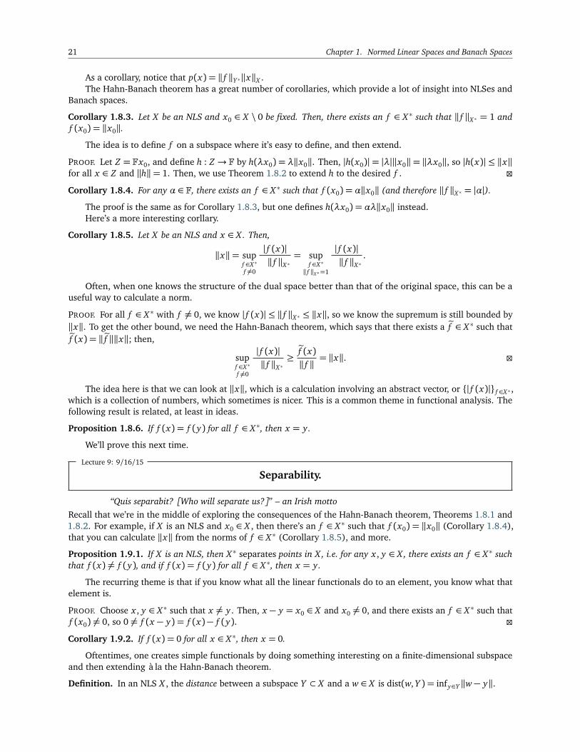
As a corollary, notice that p(x) = ‖ f ‖Y ∗‖x‖X .The Hahn-Banach theorem has a great number of corollaries, which provide a lot of insight into NLSes and
Banach spaces.
Corollary 1.8.3. Let X be an NLS and x0 ∈ X \ 0 be fixed. Then, there exists an f ∈ X ∗ such that ‖ f ‖X ∗ = 1 andf (x0) = ‖x0‖.
The idea is to define f on a subspace where it’s easy to define, and then extend.
PROOF. Let Z = Fx0, and define h : Z → F by h(λx0) = λ‖x0‖. Then, |h(x0)|= |λ|‖x0‖= ‖λx0‖, so |h(x)| ≤ ‖x‖for all x ∈ Z and ‖h‖= 1. Then, we use Theorem 1.8.2 to extend h to the desired f .
Corollary 1.8.4. For any α ∈ F, there exists an f ∈ X ∗ such that f (x0) = α‖x0‖ (and therefore ‖ f ‖X ∗ = |α|).
The proof is the same as for Corollary 1.8.3, but one defines h(λx0) = αλ‖x0‖ instead.Here’s a more interesting corllary.
Corollary 1.8.5. Let X be an NLS and x ∈ X . Then,
‖x‖= supf ∈X ∗
f 6=0
| f (x)|‖ f ‖X ∗
= supf ∈X ∗
‖ f ‖X∗=1
| f (x)|‖ f ‖X ∗
.
Often, when one knows the structure of the dual space better than that of the original space, this can be auseful way to calculate a norm.
PROOF. For all f ∈ X ∗ with f 6= 0, we know | f (x)| ≤ ‖ f ‖X ∗ ≤ ‖x‖, so we know the supremum is still bounded by‖x‖. To get the other bound, we need the Hahn-Banach theorem, which says that there exists a ef ∈ X ∗ such thatef (x) = ‖ef ‖‖x‖; then,
supf ∈X ∗
f 6=0
| f (x)|‖ f ‖X ∗
≥ef (x)‖ f ‖
= ‖x‖.
The idea here is that we can look at ‖x‖, which is a calculation involving an abstract vector, or | f (x)| f ∈X ∗ ,which is a collection of numbers, which sometimes is nicer. This is a common theme in functional analysis. Thefollowing result is related, at least in ideas.
Proposition 1.8.6. If f (x) = f (y) for all f ∈ X ∗, then x = y.
We’ll prove this next time.
Lecture 9: 9/16/15
Separability.
“Quis separabit? [Who will separate us?]” – an Irish mottoRecall that we’re in the middle of exploring the consequences of the Hahn-Banach theorem, Theorems 1.8.1 and1.8.2. For example, if X is an NLS and x0 ∈ X , then there’s an f ∈ X ∗ such that f (x0) = ‖x0‖ (Corollary 1.8.4),that you can calculate ‖x‖ from the norms of f ∈ X ∗ (Corollary 1.8.5), and more.
Proposition 1.9.1. If X is an NLS, then X ∗ separates points in X , i.e. for any x , y ∈ X , there exists an f ∈ X ∗ suchthat f (x) 6= f (y), and if f (x) = f (y) for all f ∈ X ∗, then x = y.
The recurring theme is that if you know what all the linear functionals do to an element, you know what thatelement is.
PROOF. Choose x , y ∈ X ∗ such that x 6= y . Then, x − y = x0 ∈ X and x0 6= 0, and there exists an f ∈ X ∗ such thatf (x0) 6= 0, so 0 6= f (x − y) = f (x)− f (y).
Corollary 1.9.2. If f (x) = 0 for all x ∈ X ∗, then x = 0.
Oftentimes, one creates simple functionals by doing something interesting on a finite-dimensional subspaceand then extending à la the Hahn-Banach theorem.
Definition. In an NLS X , the distance between a subspace Y ⊂ X and a w ∈ X is dist(w, Y ) = infy∈Y ‖w− y‖.

1.9. Separability: 9/16/15 22
This is nonnegative, and sometimes it’s zero even when w 6∈ Y .
Lemma 1.9.3 (Mazur Separation Thm. I). Let X be an NLS, Y ⊂ X be a subspace, and w ∈ X \ Y . Supposed = dist(w, Y )> 0. Then, there exists an f ∈ X ∗ with
• ‖ f ‖ ≤ 1,• f (w) = d, and• f (y) = 0 for all y ∈ Y .
PROOF. Let Z = Y + Fw. Then, any z ∈ Z has a unique representation as z = y + λw for exactly one choice ofy ∈ Y and λ ∈ F (which we discussed last time).
Then, define g : Z → F by g(y +λw) = λd. g is clearly linear, but it’s less clear why ‖g‖ ≤ 1.
g
y +λw‖y +λw‖
=|λ|d
‖y +λw‖=
d‖(1/λ)y +w‖
.
Since (1/λ)y ∈ Y , then ‖(1/λ)y +w‖ ≥ d, and therefore d/‖(1/λ)y +w‖ ≤ 1. Then, we use the Hahn-Banachtheorem to extend to X .
We’ll introduce another notion, entirely topological, which will be useful.
Definition. A topological space X is separable if it contains a countable dense subset, i.e. a D ⊂ X such that D = X .
A space might be large and scary, but if it’s separable, then everything is close, and therefore we can get alittle control on it.
Example 1.9.4.
(1) Q ⊂ R. Q is countable and every real number can be arbitrarily well approximated by rational numbers,so R is separable.
(2) Q(i) =Q+ iQ ⊆ C is countable and dense, so C is separable.(3) Fd is also separable, with the countable dense subset either Qd or Q(i)d .(4) If 1≤ p <∞, our Schauder basis for `p is uncountable, but we can take instead the Q(i)-span (or theQ-span if F= R) of ei∞i=1; this is a countable dense subset of `p, so `p is separable.
(5) If 1≤ p <∞, then Lp(Ω) is separable. This one is a little more surprising. The set S of simple functions(functions which are constant on a finite number of intervals) is dense in Ω, but uncountable, so wehave to restrict it in two ways: first, restrict the allowed intervals to have rational coefficients, and thenrestrict the functions to take on values in Q(i) (or Q; we’ll assume that when we talk about Q(i), thenwe mean Q for R). Thus restricted, we have our countable dense subset.
This argument doesn’t work for L∞(Ω), since simple functions aren’t dense in it, and in fact L∞(Ω) isn’tseparable.
Proposition 1.9.5. Let X be an NLS. If X ∗ is separable, then X is separable.
The converse isn’t true, because L1(Ω) is separable but L∞(Ω) isn’t. So if you start with a separable space,your dual might be bigger.
PROOF. Let fn∞n=1 be a countable, dense subset of X ∗. We’ll use this to construct a countable, dense subset of X .Since ‖ f ‖ = sup‖x‖=1| f (x)|, then we can choose for each n an xn such that ‖xn‖ = 1 and | fn(xn)| ≥ (1/2)‖ fn‖,giving us a sequence xn∞n=1.
Then, let D = spanQ(i)xn, which is still countable, and we’ll show that D = X . Suppose that it weren’t: then,there exists a w ∈ X \ D. Let d = dist(w,D) = infx∈D‖w− x‖ > 0. If we can show that ‖w− yn‖ → 0 for somesequence yn
∞n=1, then since D is closed, that would imply w ∈ D.
Since Q(i) = C (or, in the real case, Q= R),9 then D is a linear subspace of X ; thus, by Lemma 1.9.3, thereexists an f ∈ X ∗ such that f |D = 0 and f (w) = d > 0. But there’s a sequence fnk
∞k=1 such that fnk→ f . Thus,
‖ fnk− f ‖ ≥ | f (xnk
)− fnk(xnk)|= | fnk
(xnk)| ≥
12‖ fnk‖.
Since fnk− f → 0, then this means fnk
→ 0, and so f = 0. But this is a contradiction.
9Usually, Q tends to denote algebraic closure; today, we’re talking about topological closure.

23 Chapter 1. Normed Linear Spaces and Banach Spaces
So far, we’ve always looked at sets that are subspaces. Here’s an example where we don’t do that.
Definition. Let X be an NLS and C ⊆ X be a subset (not necessarily a subspace). Then, C is balanced if for anyλ ∈ F with |λ| ≤ 1 and any x ∈ C , we have λx ∈ C .
For example, if F= C, then this implies that C is invariant under rotation, as well as contractions. Note thatall subspaces are balanced.
Lemma 1.9.6 (Mazur Separation Thm. II). Let X be an NLS and C ⊆ X be a closed, convex, and balanced set. Then,for any w ∈ X \ C, there exists an f ∈ X ∗ such that | f (x)| ≤ 1 for x ∈ C and f (w)> 1.
PROOF. Since C is closed and w 6∈ C , we can choose a ball B + w about w (so B is a ball centered at the origin)such that B ∩ C = ;. Then, we can define the Minkowski functional p : X → [0,∞) by
p(x) = infn
t > 0 :xt∈ C + B
o
.
Here, C + B is a slight fattening of our set C , but we can guarantee that w 6∈ C + B. Moreover, 0 ∈ C , because C isbalanced; therefore, p(x) is always finite. We also know that p(x)≤ 1 if x ∈ C and p(w)> 1.
Moreover, p is a seminorm: since C is balaced, p(λx) = p(|λ|x) = |λ|p(x). We also have the triangle inequality,which is left to the reader.
Now, we use Theorem 1.8.2: let Y = Fw, and if f (λw) = λp(w), then f (w) = p(w) > 1, and | f (λw)| =|λ|p(w) = p(λw), so we have a nice bound. Therefore, we can extend f to an F such that F(w)> 1 and F(x)≤ 1if x ∈ C ⊂ C + B.
The key idea is the Minkowski functional; once you write that down, you’re basically done.
Lecture 10: 9/18/15
The Minkowski Functional and the Baire Category Theorem.
Last time, we had to rush through the Minkowski functional, so today we’ll talk a little more about it. This isnot a linear functional, but it does map into F, so it’s called a functional.
Specifically, given a nonempty A⊆ X , where X is an NLS, the Minkowski functional is defined as
p(x) = inft > 0 : x ∈ tA,
which takes values in [0,∞]. We then showed the following.(1) If there’s an open ball containing 0 and contained in A, then p(x) is finite.(2) p is positively homogeneous, i.e. if λ≥ 0, then p(λx) = λp(x).(3) If A is convex, then p(x + y)≤ p(x) + p(y).(4) If A is balanced, then p is a seminorm.
Well, we didn’t actually show (3), so let’s do that now. Suppose x/r, y/s ∈ A (so that r ≥ p(x) and s ≥ p(y)). Byconvexity,
x + ys+ r
=r
s+ rxr+
ss+ r
ys∈ A,
and therefore s+ r ≥ p(x + y). Since this is true for all such s and r, passing to their infimum replaces them withp(x) and p(y), so p(x) + p(y)≥ p(x + y).
This was sufficient to prove Lemma 1.9.6, but we have one more separating theorem to prove. This time, wedon’t need sets to be balanced, but we will require convexity.
Lemma 1.10.1 (Separating hyperplane theorem). Let A and B be disjoint, nonempty, convex subsets of an NLS X .(1) If A is open, then there exists an f ∈ X ∗ and a γ ∈ R such that Re( f (x))≤ γ≤ Re( f (y)) for all x ∈ A and
y ∈ B.(2) If A and B are open, the above inequality is strict.(3) If A is compact and B is closed, then the above inequality is also strict.
PROOF. We’ll prove part (1); the others are similar. Moreover, it suffices to prove it for real fields, because if F = C,then we can view X as a real vector space and get a real linear functional g that satisfies the lemma over R. Then,f (x) = g(x)− i g(i x) satisfies the lemma for C.
All right, so F= R, and A is open and both are convex. We’ll have to put the Minkowski functional into thisproof somehow, so let’s start by picking an x ∈ A and a y ∈ B. Let A− x = t − x : t ∈ A, and define B− y similarly.
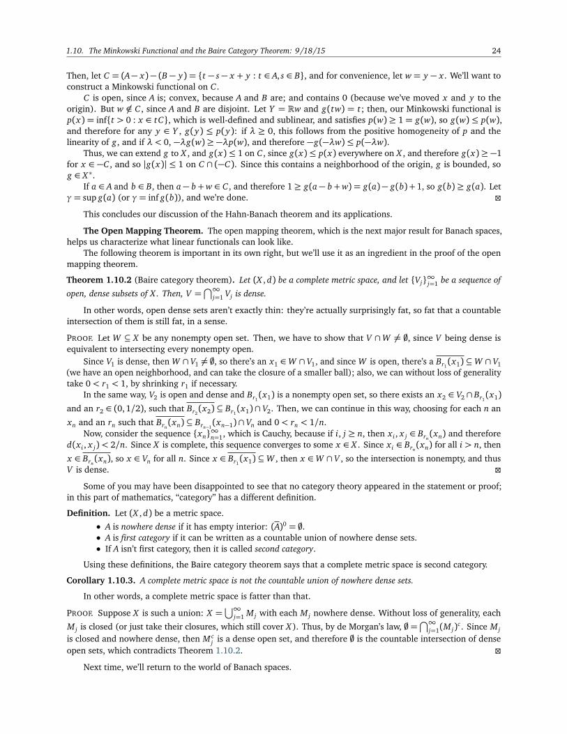
1.10. The Minkowski Functional and the Baire Category Theorem: 9/18/15 24
Then, let C = (A− x)− (B − y) = t − s− x + y : t ∈ A, s ∈ B, and for convenience, let w= y − x . We’ll want toconstruct a Minkowski functional on C .
C is open, since A is; convex, because A and B are; and contains 0 (because we’ve moved x and y to theorigin). But w 6∈ C , since A and B are disjoint. Let Y = Rw and g(tw) = t; then, our Minkowski functional isp(x) = inft > 0 : x ∈ tC, which is well-defined and sublinear, and satisfies p(w) ≥ 1 = g(w), so g(w) ≤ p(w),and therefore for any y ∈ Y , g(y) ≤ p(y): if λ ≥ 0, this follows from the positive homogeneity of p and thelinearity of g, and if λ < 0, −λg(w)≥ −λp(w), and therefore −g(−λw)≤ p(−λw).
Thus, we can extend g to X , and g(x)≤ 1 on C , since g(x)≤ p(x) everywhere on X , and therefore g(x)≥ −1for x ∈ −C , and so |g(x)| ≤ 1 on C ∩ (−C). Since this contains a neighborhood of the origin, g is bounded, sog ∈ X ∗.
If a ∈ A and b ∈ B, then a− b+w ∈ C , and therefore 1≥ g(a− b+w) = g(a)− g(b) + 1, so g(b)≥ g(a). Letγ= sup g(a) (or γ= inf g(b)), and we’re done.
This concludes our discussion of the Hahn-Banach theorem and its applications.
The Open Mapping Theorem. The open mapping theorem, which is the next major result for Banach spaces,helps us characterize what linear functionals can look like.
The following theorem is important in its own right, but we’ll use it as an ingredient in the proof of the openmapping theorem.
Theorem 1.10.2 (Baire category theorem). Let (X , d) be a complete metric space, and let Vj∞j=1 be a sequence of
open, dense subsets of X . Then, V =⋂∞
j=1 Vj is dense.
In other words, open dense sets aren’t exactly thin: they’re actually surprisingly fat, so fat that a countableintersection of them is still fat, in a sense.
PROOF. Let W ⊆ X be any nonempty open set. Then, we have to show that V ∩W 6= ;, since V being dense isequivalent to intersecting every nonempty open.
Since V1 is dense, then W ∩ V1 6= ;, so there’s an x1 ∈W ∩ V1, and since W is open, there’s a Br1(x1) ⊆W ∩ V1
(we have an open neighborhood, and can take the closure of a smaller ball); also, we can without loss of generalitytake 0< r1 < 1, by shrinking r1 if necessary.
In the same way, V2 is open and dense and Br1(x1) is a nonempty open set, so there exists an x2 ∈ V2 ∩ Br1
(x1)and an r2 ∈ (0, 1/2), such that Br2
(x2) ⊆ Br1(x1)∩ V2. Then, we can continue in this way, choosing for each n an
xn and an rn such that Brn(xn) ⊆ Brn−1
(xn−1)∩ Vn and 0< rn < 1/n.Now, consider the sequence xn∞n=1, which is Cauchy, because if i, j ≥ n, then x i , x j ∈ Brn
(xn) and therefored(x i , x j)< 2/n. Since X is complete, this sequence converges to some x ∈ X . Since x i ∈ Brn
(xn) for all i > n, then
x ∈ Brn(xn), so x ∈ Vn for all n. Since x ∈ Br1
(x1) ⊆W , then x ∈W ∩ V , so the intersection is nonempty, and thusV is dense.
Some of you may have been disappointed to see that no category theory appeared in the statement or proof;in this part of mathematics, “category” has a different definition.
Definition. Let (X , d) be a metric space.
• A is nowhere dense if it has empty interior: (A)0 = ;.• A is first category if it can be written as a countable union of nowhere dense sets.• If A isn’t first category, then it is called second category.
Using these definitions, the Baire category theorem says that a complete metric space is second category.
Corollary 1.10.3. A complete metric space is not the countable union of nowhere dense sets.
In other words, a complete metric space is fatter than that.
PROOF. Suppose X is such a union: X =⋃∞
j=1 M j with each M j nowhere dense. Without loss of generality, each
M j is closed (or just take their closures, which still cover X ). Thus, by de Morgan’s law, ;=⋂∞
j=1(M j)c . Since M j
is closed and nowhere dense, then M cj is a dense open set, and therefore ; is the countable intersection of dense
open sets, which contradicts Theorem 1.10.2.
Next time, we’ll return to the world of Banach spaces.
25 Chapter 1. Normed Linear Spaces and Banach Spaces
Lecture 11: 9/21/15
The Open Mapping Theorem.
Last time, we learned about the Baire category theorem. Today, we’ll use it to prove the open mappingtheorem.
Definition. A continuous map f : X → Y is open if it maps open sets to open sets, i.e. if U ⊆ X is open, thenf (U) ⊆ Y is open.
An arbitrary continuous map is not open; for example, T : R2 → R2 sending (x , y) 7→ (x , 0) is perfectlycontinuous, but the image of B1(0) is (0,1)× 0, which isn’t open in R2. Surjective linear maps, however, areopen.
In the infinite-dimensional case, things can become more interesting; for example, T : `2 → `2 sendingen→ (1/n)en isn’t open (the image of the unit ball isn’t open), but is linear and surjective; the discrepancy is thatthis T isn’t bounded.
Theorem 1.11.1 (Open mapping). Let X and Y be Banach and T : X → Y be a bounded, linear surjection. Then, Tis an open map.
A bounded linear map is typical in this class, so the key hypothesis in this theorem is that T is surjective. Theexample (x , y) 7→ (x , 0) shows that this is important.
This is a pretty fundamental theorem about Banach spaces.
PROOF. It suffices to show that T(B1(0)) contains a Br(0) for some r > 0: if U ⊂ X is open, then to check thatT (U) is open, we can pick a y ∈ T (U) and a preimage x (i.e. T (x) = y). Then, we can look at U − x , and sinceT is linear, then T(U − x) = T(U) − y. But since x and y are now sent to the origin, we just need to pick aneighborhood of x and make sure its image contains a neighborhood of y .
This is the proper way to think about the theorem: if you know what a bounded linear map looks like at theorigin, you know what it looks like everywhere.
Since T is onto, then we can write
Y =∞⋃
j=1
T (B j(0)).
Since Y is a complete metric space, then the Baire category theorem tells us it’s not the union of nowhere densesets. Thus, there’s some k such that T (Bk(0)) isn’t nowhere dense, i.e. there’s an open W1 ⊂ T (Bk(0)). Thus, wecan scale: (1/2k)W ⊆ (1/2k)T (Bk(0)) = T (B1/2(0)).
Since W1 is open, there’s a y0 ∈ Y and an r > 0 such that Br(y0) ⊆W ⊆ T (B1/2(0)). This is almost everything:
Br(0) = Br(y0)− y0
⊆ Br(y0)− Br(y0)
⊆ T (B1/2(0)) + T (B1/2(0))
⊆ T (B1(0)),
by the triangle inequality. We’d be done, except that we had to take the closure (which ultimately came from theBaire category theorem). Thus, we’ll show that if ε > 0, then T (B1+ε(0)) ⊇ Br(0), because then
T (B1(0)) =1
1+ εT (B1+ε(0)) ⊇ Br/(1+ε)(0).
Then, we won’t need the closure anymore. Note that this isn’t obvious, even if it seems obvious in the finite-dimensional case.
Fix a y ∈ Br(0) and an ε > 0. We know that T (B1(0))∩ Br(0) is dense in Br(0) (since we showed already itsclosure contains Br(0)), so we can pick an x1 ∈ B1(0) such that ‖y − T x1‖< ε/2.
Inductively, when n≥ 1, suppose we’ve picked x1, . . . , xn such that ‖x1‖ ≤ 1 and ‖x j‖ ≤ 2− j+1ε and ‖y−T (x1+· · ·+xn)‖< 2−nεr. Let z = y−T (x1+· · ·+xn), so that z ∈ B2−nεr(0). Since T (B1(0))∩Br(0) is dense in Br(0), we canscale things: there’s an xn+1 ∈ B2−nε(0) such that ‖z−T xn+1‖ ≤ 2−(n+1)εr; thus, ‖y−T (x1+· · ·+xn+1)‖ ≤ 2−(n+1)εr.
1.11. The Open Mapping Theorem: 9/21/15 26
Since the terms get smaller and smaller,∑n
j=1 x j is a Cauchy sequence, so since X is complete, then this sumconverges to a point x ∈ X , such that
‖x‖ ≤ 1=∞∑
j=2
‖x j‖< 1+∞∑
n=2
2−n+1ε = 1+ ε.
Since T is continuous, then Tsn→ T x = y .
The first part, showing it’s true for T (B1(0)), is pretty easy, but then getting just one more ε is surprisinglyfussy.
Corollary 1.11.2. If X and Y are Banach spaces and T : X → Y is a bounded, linear bijection (one-to-one and onto),then the inverse map exists and is a bounded linear functional.
In other words, the inverse of a bounded linear functional is bounded linear. This is nice, and very useful.
PROOF. It’s easy to show T−1 is linear. T is open, so it takes open sets to open sets, and therefore for T−1, thepreimage of every open set is open, so T−1 is continuous.
We now know enough to make the following definition.
Definition. If X and Y are Banach spaces, we say that they’re isomorphic as Banach spaces if there exists a linear,bounded bijection T : X → Y . If in addition T preserves the norm, it’s called a isometry.
This means that X and Y have the same vector space structure (since there’s a bijective linear map) andsame topology (there’s a homeomorphism). If T isn’t an isometry, then the norms may be different, but they’ll beequivalent, so X and Y are basically the same.
There’s a closely related result about graphs of maps; we could have proven this first and used it to derive theopen mapping theorem, though we’ll go about it in the other direction.
Definition. Let X and Y be topological spaces, D ⊆ X and f : D → Y . Then, the graph of f is graph( f ) =(x , f (x)) : x ∈ D ⊆ X × Y .
X × Y is where we’re used to drawing graphs (such as X , Y = R); we chose D because the function might notbe defined everywhere.
Proposition 1.11.3. Let X be a topological space, Y be a Hausdorff space, and f : X → Y be continuous. Then,graph( f ) is closed in X × Y .
In the case of graphs we’re most familiar with, this makes sense, as it’s how we’re used to thinking of continuityintuitively.
PROOF. Let U = X × Y \ graph( f ), and let (x0, y0) ∈ U , so f (x0)≤ y0.Recall that since Y is Hausdorff, we can choose open neighborhoods V and W in Y around y0 and f (x0),
respectively, that don’t intersect. Then, we’re going to consider f −1(W ) ⊂ X ; specifically, f −1(W )× V doesn’tintersect graph( f ), and is an open neighborhood of (x0, y0).
If that proof didn’t make sense, drawing a picture will likely help.
Definition. Let X and Y be NLSes, D ⊆ X be a linear subspace, and T : D→ Y be linear. Then, we say that T is aclosed operator if graph(T ) is closed in X × Y .
An open map takes open sets to open sets; a bounded map takes bounded sets to bounded sets; but a closedoperator doesn’t take closed sets to closed sets. This can be confusing.
If X and Y are metric spaces and f : D→ Y is continuous, then graph( f ) being closed means that if xn∞n=1 ⊂ D
is such that xn→ x and T xn→ y , then x ∈ D and y = T x .
Theorem 1.11.4 (Closed graph theorem). Let X and Y be Banach spaces, and T : X → Y be linear. Then, T isbounded iff it’s closed.
27 Chapter 1. Normed Linear Spaces and Banach Spaces
PROOF. The forward direction is true in general (continuous implies closed).In the other direction, suppose graph(T ) is closed, and therefore is a closed linear subspace of X × Y . This is a
very important point: since X and Y are Banach, then X × Y is Banach, and since graph(T) is closed in it, thengraph(T ) is also a Banach space, with the graph norm10
‖(x , T x)‖= ‖x‖X + ‖T x‖Y .
Define two projection operators π1 : (x , y) 7→ x and π2 : (x , y) 7→ y , so that we have maps
graph(T )π2
π1
X Y.
π1 is a linear bijection between Banach spaces, and is bounded (by the triangle inequality, ‖x‖X ≤ ‖(x , T x)‖+‖T x‖Y ), so by Corollary 1.11.2, its inverse π−1
1 is a bounded linear functional. Moreover, π2 is bounded linear forthe same reasons, so T = π2 π−1
1 is bounded as well.
Lecture 12: 9/23/15
The Uniform Boundedness Principle.
Recall that last time, we proved the closed graph theorem, Theorem 1.11.4, which states that if X and Y areBanach spaces and T : X → Y is linear, then T has a closed graph iff it’s bounded.
Corollary 1.12.1. Let X and Y be Banach spaces, D ⊂ X be a subspace, and T : D→ Y be closed. Then, T is boundediff D is closed.
PROOF. In the reverse direction, if D is closed, then it’s Banach, so we can apply Theorem 1.11.4.Conversely, suppose T is bounded, and let xn∞n=1 ⊂ D be such that xn → x in X . Since T is bounded and
linear, then T xn∞n=1 is Cauchy.11
Since Y is complete, then T xn→ y for some y ∈ Y . And since T is a closed operator, then graph(T ) = (x , T x)is closed. Since xn→ x and T xn→ y, then (x , y) ∈ graph(T ), so y = T x and thus x ∈ D. Therefore D containsits limit points, and so is closed.
Hopefully this illustrates some uses of the closed graph theorem.
Example 1.12.2. Though continuous implies closed, the converse isn’t true. Here’s an example. Let X = C([0, 1]),the continuous functions with the L∞ norm, and let D = C1([0,1]) ⊂ X , the C1 functions. Let T : D→ X be thederivative operator, so T ( f ) = f ′.
This is perfectly well defined: if f is C1, then f ′ is continuous. Then, D 6= X (e.g. f (x) = |x − 1/2|), butD = X , so D is not closed in X (intuitively, any continuous but not differentiable function can be well approximatedby a C1 function).
• First, we’ll see that T isn’t continuous (equiv. bounded). T(xn) = nxn−1, but ‖xn‖ = 1 and ‖T xn‖ =n→∞.
• However, it is closed. Let fn∞n=1 ⊆ D have a limit fn→ f in X , and such that f ′n → g in X . We want toshow that g = f ′. This follows from the fundamental theorem of calculus: for each n,
fn(t) = f0(t) +
∫ t
0
f ′n(τ)dτ.
Since convergence in L∞ implies pointwise convergence. Then, by the dominated convergence theorem,these integrals also converge (recall that continuous functions on compact sets are bounded), so
f (t) = f (0) +
∫ t
0
g(τ)dτ= f (0) +
∫ τ
0
f ′(τ)dτ.
Thus, f ′(t) exists and g = f ′, so f ∈ C1([0, 1]).10Though this was defined in a way mirroring the `1 norm, you can use the analogous definition with any `p including `∞, since, as we
proved on a problem set, they’re all equivalent.11This is because ‖T xn − T xm‖= ‖T (xn − xm)‖= ‖T‖‖xn − xm‖ → 0.
1.12. The Uniform Boundedness Principle: 9/23/15 28
Continuous is better than closed, but closed is part of the way there, in some sense.We’ve talked about two of the three important theorems about NLSes: the Hahn-Banach theorem and the
open mapping theorem. Here’s the third.
Theorem 1.12.3 (Uniform boundedness principle). Let X be Banach, Y be an NLS, and Tαα∈I ⊂ B(X , Y ). Then,one of the following holds.
(1) The collection is uniformly bounded: there’s an M such that supα∈I‖Tα‖B(X ,Y ) ≤ M.(2) There’s a point where they’re not: there’s an x ∈ X such that supα∈I‖TαX‖=∞.
The point is, if these functions aren’t uniformly bounded, then they all blow up at some given point, when apriori they could do so in different places. This is true no matter how large the collection I is; it could very well beuncountable.
The proof in the notes is nice, but a little fussy to prove, and uses the Baire category theorem. We’ll give aproof based on the following lemma, which is a little nicer.
Lemma 1.12.4. Let X and Y be NLSes and T : X → Y be a bounded linear map. For any x ∈ X and r > 0,supy∈Br (x)‖T y‖ ≥ r‖T‖.
The idea is if x = 0, we have equality, but even if we don’t, this is still a one-sided bound.
PROOF. For a visualization, it may help to think about the case X = Y = R, where graph(T) is a line with slope‖T‖ through the origin. Here, supy∈Br (x)‖T y‖= ‖T‖(‖x‖+ r)≥ ‖T‖r.
More generally, we’ll think of the “larger” and “smaller” parts of Br(x). The triangle inequality tells us thatsince z = (1/2)(x + z)− (x − z), then
‖Tz‖ ≤12(‖T (x + z)‖+ ‖T (x − z)‖)
≤max‖T (x + z)‖,‖T (x − z)‖.
If we take the supremum over z ∈ Br(0), we know that
r‖T‖ ≤ supz∈Br (0)
‖T (x + z)‖= supy∈Br (x)
‖T y‖.
This is a nice geometric result, and relatively easy to prove. Then, we’ll use it to attack the uniform boundednessprinciple.
PROOF OF THEOREM 1.12.3. Since we want to show one of two things is true, let’s assume supα‖Tα‖ =∞. Choosea countable subcollection Tn
∞n=1 such that ‖Tn‖ ≥ 4n. Then, choose x0 = 0 ∈ X and choose xn ∈ X such that
‖xn − xn−1‖ ≤ 3−n (so that xn ∈ B3−n(xn−1)), so that by Lemma 1.12.4, ‖Tn xn‖ ≥ (2/3)3−n‖Tn‖.Since xn is Cauchy, then it converges to some x ∈ X , and ‖x − xn‖ ≤ (1/2)3−n, since
‖x − xn‖= limm→∞
‖xm − xn‖
≤ limm→∞
n+1∑
j=m
‖x j − x j−1‖
≤ limm→∞
3−m + 3−(m−1) + · · ·+ 3−(n+1)
≤ limm→∞
3−n∞∑
k=1
13
k
=12
3−n,
since it’s a nice old geometric series.Finally, we’re going to look at Tn x .
‖Tn x‖ ≤ ‖Tn(x − xn)‖+ ‖Tn xn‖ ≤ ‖Tn‖‖x − xn‖+ ‖Tn x‖.
Thus, we know that23
3−n‖Tn‖ ≤ ‖Tn‖12
3−n + ‖Tn x‖,
and therefore
‖Tn x‖ ≥16
3−n‖Tn‖ ≥13
43
n
,
which goes to infinity.
29 Chapter 1. Normed Linear Spaces and Banach Spaces
The Double-Dual. If X is an NLS, then X ∗ = B(X ,F) is a Banach space, and we can form the double-dualX ∗∗ = B(X ∗,F), which is also a Banach space. It’s possible to interpret X as sitting inside X ∗∗.
For any x ∈ X , define the evaluation map Ex : X ∗ → F by Ex( f ) = f (x): that is, we evaluate f at x . Sincef : X → F, then Ex is well-defined, and it’s linear: if f , g ∈ X ∗ and λ ∈ F, then
Ex( f + g) = ( f + g)(x) = f (x) + g(x) = Ex( f ) + Ex(g)
Ex(λ f ) = (λ f )(x) = λ( f (x)) = λEx( f ).
Ex is also bounded, which is more interesting. If you think about what the norm means, then
‖Ex‖X ∗∗ = supf ∈X ∗
f 6=0
|Ex( f )|‖ fX ∗‖
= supf ∈X ∗
f 6=0
f (x)‖ f ‖X ∗
= ‖x‖X ,
where the last equality is due to Corollary 1.8.5.
Definition. Let (M , d) and (N ,ρ) be metric spaces. Then, f : M → N is an isometry if ρ( f (x), f (y)) = d(x , y)for all x , y ∈ M . If f is surjective, M and N are said to be isometric.
Note that f is always injective, because if f (x) = f (y), then ρ( f (x), f (y)) = 0 = d(x , y), so x = y. Thus,isometric spaces are given by a bijection f .
Anyways, that’s what’s going on here: not only is the metric the same, but the norm is the same. We have a mapE : X → X ∗∗ sending x 7→ Ex . E is a bounded linear map, and an isometry. Therefore, eX = Ex ∈ X ∗∗ : x ∈ X ⊂ X ∗∗
is isomorphic and isometric to X . It might not be all of X ∗∗, but we’ve embedded X into its double-dual.
Definition. Sometimes, X = X ∗∗ (i.e. eX = X ∗∗). If this is true, X is said to be reflexive.
In general, X ⊆ X ∗∗ ⊆ X ∗∗∗∗ ⊆ · · · ; if X = X ∗∗, then this entire chain collapses to equalities. Similarly, we couldhave started with X ∗ and X ∗∗∗, and so on.
Theorem 1.12.5. If X is reflexive, then X ∗ is reflexive.
This is left to the exercises, but isn’t hard to prove. Notice, however, that the converse isn’t true.
Example 1.12.6. If 1≤ p <∞, we know that (`p)∗ = `q, so `p is reflexive for 1< p <∞. `1 and `∞ aren’t asnice, so we don’t have reflexivity. (The duality follows from something on the homework this week.)
Since (Lp(Ω))∗ = Lq(Ω) for 1 < p <∞, then Lp(Ω) is reflexive (which follows from the Radon-Nikodymtheorem). Similarly, L1(Ω) and L∞(Ω) are more complicated.
Lecture 13: 9/25/15
Weak and Weak-∗ Convergence.
In a finite-dimensional NLS, we know that we’re basically looking at Fd , where we have the Heine-Boreltheorem: a set is closed and bounded iff it’s compact. But, of course, infinite dimensions are weirder, and in factthe unit ball isn’t compact in an infinite-dimensional vector space. This was the reasoning behind one of the lessintuitive HW problems, about embedding infinitely many disjoint balls of a fixed radius into the unit ball.
Theorem 1.13.1. Let Y ⊆ X be a closed subspace, and Z be another subspace containing Y . If Z 6= Y and θ ∈ (0, 1),then there exists a z ∈ Z such that ‖z‖= 1 and dist(z, Y ) = θ .
The intuition in the finite-dimensional case is that z should be “orthogonal” to Y , but not all infinite-dimensionalspaces have an inner product structure (which is what gives us angles), so we have to be careful.
PROOF. Pick a z0 ∈ Z \ Y and let
d = dist(z0, Y ) = infy∈Y‖y − z0‖.

1.13. Weak and Weak-∗ Convergence: 9/25/15 30
Since Y is closed, d > 0, so we can choose a y0 ∈ Y such that d/θ ≥ ‖z0−y0‖ ≥ d. Then, let z = (z0−y0)/‖z0−y0‖ ∈Z . For all y ∈ Y ,
‖z − y‖=‖z0 −
y1∈Y︷ ︸︸ ︷
y0 − y‖z0 − y0‖‖‖z0 − y0‖
=‖z0 − y1‖‖z0 − y0‖
≥ ‖z0 − y1‖θ
d≥ θ .
Corollary 1.13.2. If X is an infinite-dimensional NLS and M ⊂ X is a closed, bounded set with nonempty interior,then M is not compact.
The Heine-Borel theorem is false in infinite dimensions. Alas.
PROOF. It’s sufficient to show it for the (closed) unit ball, because then translations and scalings cover all suchclosed, bounded sets.
Let x1 ∈ X with ‖x1‖ = 1, and we’ll inductively assume we’ve chosen x1, . . . , xn such that ‖x i‖ = 1 and‖x i − x j‖ ≥ 1/2 for all i 6= j. Let Y = spanx1, . . . , xn, so since Y is finite-dimensional and X is infinite-dimensional, we can choose an x ∈ X \ Y and let Z = spanx , Y . With θ = 1/2, Theorem 1.13.1 gives us anxn+1 ∈ Z with ‖xn+1‖= 1 and dist(xn+1, Y )≥ 1/2.
Thus, we can pick an infinite sequence of points on the unit sphere such that all of them are at least distance1/2 from each other. Thus, xn is bounded, but has no convergent subsequence, so B1(0) cannot be compact.12
A modification of this proof shows that the volume is arbitrarily large too, not just the surface area.What we’ll do about this is to define a new topology, which is weaker (has fewer open sets); since compactness
is a condition on open covers, this makes things more likely to be compact. We’ll start with a new notion ofconvergence, and then extract the topology afterwards.
Definition. Let X be an NLS and xn∞n=1 ⊂ X .
• We say that xn converges weakly to x , written xn * x or xnw→ x , if for any f ∈ X ∗, f (xn)→ f (x).
• If fn∞n=1, then fn converges weak-∗ (said “weak-star”) to f , written fnw∗→ f , if for all x ∈ X , f (xn)→ f (x).
As a contrast, xn→ x given by ‖xn − x‖ → 0 is sometimes called strong convergence.So in a space X ∗ that’s the dual of some X , we have three notions of convergence floating around: the strong
topology ‖ fn − f ‖X ∗ → 0, the weak topology F( fn)→ F( f ) for all F ∈ X ∗∗, and weak-∗, where we only considerevaluation maps in X ∗∗.
These notions of convergence represent new topologies. Let’s establish some propositions before we continue.
Proposition 1.13.3. If xn→ x as n→∞ (i.e. it converges strongly), then xn * x.
This is obvious: ‖xn − x‖ → 0, and any f ∈ X ∗ is continuous in the strong topology, so ‖ f (x − xn)‖ → 0 too.
Example 1.13.4. The converse is not true: weak convergence does not imply strong convergence. Let 1< p <∞and consider `p, with our Schauder basis en∞n=1. This sequence does not converge strongly, because
‖en − em‖`p =
∞∑
i=1
|eni − em
i |p
1/p
= 21/p,
which does not go to zero. But en * 0! Take any f ∈ (`p)∗ = `q; then, f (en) =∑
fieni = fn, and since
∑
| fn|q1/q
is finite, then | fn| → 0.
This is clearly a very different kind of convergence than strong convergence, but we have more thingsconverging, which is nice if you like convergence. It’s in some sense a sampling notion.
12Here, we’re using the theorem that compactness is equivalent to sequential compactness in metric spaces, and we should also remarkthat no subsequence of xn converges, which is the criterion we need.
31 Chapter 1. Normed Linear Spaces and Banach Spaces
Proposition 1.13.5. Let X be an NLS, xn ⊂ X and fn ⊂ X ∗. Then:
• If xn converges weakly, then the limit is unique and ‖xn‖ is bounded.• If fn converges weak-∗, then the limit is unique. If in addition X is Banach, then ‖ fn‖ is bounded.
PROOF. Suppose xn * x and xn * y . Therefore for any f ∈ X ∗, f (xn)→ f (x) and f (xn)→ f (y). But since limitsare unique in F, then f (x) = f (y), so since this is true for all f ∈ X ∗, then x = y .
Fix an f ∈ X ∗, so that f (xn)∞n=1 converges in F, and therefore is bounded. Thus, |Ex( f )|= | f (xn)| ≤ C f forall n (i.e. some constant C that depends only on f ). In particular, Exn
∞n=1 ⊆ X ∗∗ is pointwise bounded, so by theuniform boundedness principle, ‖xn‖= ‖Exn
‖ ≤ C .The second part is left as an exercise; but since uniform boundedness requires the space to be Banach, we’ll
have to assume that of X .
Proposition 1.13.6. Let X be an NLS and xn * x. Then, ‖x‖ ≤ lim infn→∞‖xn‖.
This one was left as an exercise.Though most of the time one only cares about convergence, the topologies are worth knowing about. Recall
that a topology is a collection of open sets, so one topology being “smaller” than another means that it’s a subsetof the other collection of open sets.
Definition. The weak topology on X is the smallest topology such that each f ∈ X ∗ is continuous. The weak-∗topology on X ∗ is the smallest topology such that each Ex (the image of x in the canonical map X → X ∗∗) iscontinuous.
Since we know these are continuous in the strong topology, these are smaller topologies; there are fewer opensets, and convergence is nicer.
What this means is that if U ⊂ F is open and f ∈ X ∗, then f −1(U) is open in X . Since these f are linear, thenwe really only need to talk about open sets containing 0, and therefore contain an open ball Bε(0), which will giveus all the open sets in the weak topology (by translation).
We know that if fi ∈ X ∗, then f −1i (Bεi
(0)) is open, and we can take arbitrary unions and finite intersections.Specifically, our basic open sets are translates of sets of the form
n⋂
i=1
f −1i
Bεi(0)
.
All open sets in the weak topology are translations of unions of these sets, which can be rewritten as
U = x ∈ X : | fi(x)|< εi , i = 1, . . . , n.
For the weak-∗ topology, the basic opens are the translates of
V = f ∈ X ∗ : | f (x i)|< εi , i = 1, . . . , n
=n⋂
i=1
E−1x i(Bεi(0)).
The next thing we need to do is show that these topologies imply the notions of convergence we defined at thestart of lecture.
Lecture 14: 9/28/15
The Banach-Alaoglu Theorem.
“Just take these epsilons; don’t worry about it. . . ”
Recall that we’ve defined weak convergence xn * x if f (xn)→ f (x) for all f ∈ X ∗, and an even weaker notion
called weak-∗ convergence where fnw∗→ f if fn(x)→ f (x) for all x ∈ X . Then, we defined the weak and weak-∗
topologies: the smallest topologies on X (resp. X ∗) such that every f ∈ X ∗ (resp. Ex ∈ X ∗∗) is continuous.We saw that the basic open sets in the weak topology are (the translates of) finite intersections of sets of the
form f −1i (Bεi
(0)) for fi ∈ X ∗; in other words, a set of points where fi(x) < εi for some finite number of fi ∈ X ∗
and εi > 0. General open sets are unions of translations of these sets. We also had a similar notion for the weak∗topology.
1.14. The Banach-Alaoglu Theorem: 9/28/15 32
Proposition 1.14.1. Let X be an NLS and xn∞n=1 ⊆ X . Then, xn → x in the weak topology iff xn * x, and if
fn∞n=1 ⊆ X ∗, then fn→ f in the weak∗ topology iff fn
w∗→ f .
PROOF. For the first part and in the forward direction, suppose f ∈ X ∗, so that f is continuous in the weak topology.Thus, limn→∞ f (xn) = f (x), so xn * x .
Conversely, suppose xn * x , and let U be a basic open set about x , so that
U = x + y ∈ X : | fi(y)|< εi , i = 1, . . . , n
for some fi ∈ X ∗ and εi > 0. Since f (xn) → f (x) for all f , then there’s an N > 0 such that | fi(xn − x)| =| fi(xn)− fi(x)|< εi for all i = 1,2, . . . , n, and therefore xn = (xn − x) + x ∈ U .
The proof of the second part is similar.
Remark.• The Hahn-Banach theorem implies that the weak topology is Hausdorff, since it implies there’s a linear
functional that separates any two points.• If τw denotes the (collection of open sets of the) weak topology, and τ denotes the strong topology, thenτw ⊂ τ (i.e. it actually is weaker): since each fi is continuous in the strong topology, then inverse imagesof open sets under it remain open. A similar result holds for the weak-∗ topology.
Theorem 1.14.2 (Banach-Alaoglu13). Let X be an NLS and B∗1 = f ∈ X ∗ : ‖ f ‖X ∗ ≤ 1 be the closed unit ball in X ∗.Then, B∗1 is compact in the weak-∗ topology.
PROOF. Let Bx = λ ∈ F : |λ| ≤ |x |. Then, each Bx is a closed and bounded subset of F, and therefore compact,and let C =
∏
x∈X Bx . By Tychonoff’s theorem, which is an amazing theorem, any product of compact sets is stillcompact, so C is compact, even though it’s (in some sense) huge!14 A function g : X → F such that |g(x)| ≤ ‖x‖,whether it’s linear or not, can be viewed as an element of C by sending g 7→ (g(x))x∈X . Then, the coordinatemap πx : C → Bx sends g 7→ g(x), so it’s just the evaluation map, and we know by the definition of the producttopology that this map is continuous. In particular, this defines a continuous inclusion of B∗1 ⊆ C , where the formerhas the weak-∗ topology. Since C is compact, then B∗1 is compact if it’s closed in C .
We probably won’t get around to showing it, but the weak and weak-∗ topologies aren’t metrizable, so the niceproof techniques from metric spaces don’t work, and we’ll have to use more basic topological methods. Specifically,we’ll have to show that all accumulation points of B∗1 are in B∗1.
Let g be an accumulation point of B∗1, and fix x , y ∈ X and a λ ∈ F; then, let
U = g + h ∈ C : |h(x i)|< ε, i = 1, . . . , m.
Specifically, we’ll take m= 4 and the points x i = x , y , x + y , and λx . If f = g + h ∈ B∗1, we’ll choose the epsilons|h(x)|< ε/3max(1, |λ|), |h(y)< ε/3, |h(x + y)|< ε/3, and |h(λx)|< 2ε/3, for some arbitrary ε > 0. Then,
|g(x + y)− g(x)− g(y)|= |h(x + y)− h(x)− h(y)|≤ |h(x + y)|+ |h(x)|+ |h(y)|< ε.
|g(λx)−λg(x)|= h(λx)−λh(x)|< ε.
This is why we chose the strange epsilons; as ε→ 0, this forces g to be linear! Moreover,
|g(x)|= | f (x)− h(x)| ≤ ‖ f ‖+ |h(x)| ≤ 1+ε
3,
so in particular ‖g‖ ≤ 1, so g ∈ B∗1, and so B∗1 has to be compact.
Now, we can begin to unpack the applications of this theorem. Even though these topologies aren’t metrizable,we can get some nice topological results for suitably nice spaces.
Theorem 1.14.3. Let X be a separable Banach space and K ⊆ X ∗ be weak-∗ compact. Then, K with the weak-∗topology is metrizable.
In particular, on this set, sequential compactness is equivalent to compactness, which can be useful!
13Pronounced approximately “ala-glue.”14Note that this compactness is in the product topology, not the box topology. If Xαα∈I is a set of topological spaces and X =
∏
α∈I Xα,then for each α there’s a coordinate map πα : X → Xα sending each element to its coordinate in that index. Then, the product topology isdefined to be the smallest topology in which each of these coordinate maps is continuous.

33 Chapter 1. Normed Linear Spaces and Banach Spaces
PROOF. Let D = xn∞n=1 ⊆ X be a countable, dense subset of X . Then, the evaluation maps En = Exn
are weak-∗continuous; since D is dense, then these En separate points. That is, if En( f ∗) = En(g∗) for all n (i.e. f ∗(xn) = g∗(xn)for all n), then f ∗ = g∗.
Let cn = sup f ∗∈K |En( f ∗)|, which is a continuous, finite function on a compact set and therefore has a maximum,and let
fn =
En
cn, cn 6= 0
0, cn = 0.
Now that we’ve scaled suitably, we may define our metric: let
d( f ∗, g∗) =∞∑
n=1
2−n| fn( f∗)− fn(g
∗)|.
This is a metric: it’s clearly symmetric, and it’s 0 iff each term is, which is true iff f ∗ = g∗, as observed above.Moreover, since the triangle inequality holds termwise, then it holds here.
However, we still need to prove that the topology τd induced by this metric agrees with the weak-∗ topologyτ on K . First, we’ll show that τd ⊆ τ: for N ≥ 1, let
dN ( f∗, g∗) =
N∑
n=1
2−n| fn( f∗)− fn(g
∗)|,
and consider dN (·, g∗) : X ∗→ [0,∞) sending f ∗ 7→ dN ( f ∗, g∗). This is weak-∗ continuous, and dN (·, g∗)→ d(·, g∗)converges uniformly, so the limit d(·, g∗) is continuous. Therefore Br(g∗) = f ∗ ∈ K : d( f ∗, g∗)< r is the inverseimage of (−∞, r) (which is open in R) under d(·, g∗), which is continuous, so it’s open, and thus τd ⊆ τ (sincethese balls generate all opens).
Conversely, let A ∈ τ, so that Ac ⊂ K is τ-closed, and therefore τ-compact. Since we already showed thatτd ⊆ τ, then Ac must be τd -compact (as there are fewer open sets), and in particular τd -closed. Thus, A is open inτd .
Lecture 15: 9/30/15
The Generalized Heine-Borel Theorems.
Recall that we proved the Banach-Alaoglu theorem, that the unit ball in X ∗ is weak-∗ compact. This isn’t superuseful, but we found that if X is a separable Banach space, then B∗1 is a metric space. Relatedly, since any weak-∗compact subspace of X ∗ is metrizable, then if fn ⊂ X ∗ and ‖ fn‖ ≤ C , then there exists a subsequence fnk
whichweak-∗ converges to an f ∈ X ∗.
In other words, we know the following.
Theorem 1.15.1 (Generalized Heine-Borel I). Let X be a separable Banach space and K ⊆ X ∗. Then, the followingare equivalent.
(1) K is weak-∗ compact.(2) K is weak-∗ closed and bounded.(3) K is weak-∗ sequentially compact.15
We’ve already seen that (1) =⇒ (3), and the discussion above is (2) =⇒ (1) for the unit ball (whichgeneralizes by scaling to any ball, and therefore to any bounded set, since it can be contained in a large ball). Sothere’s only one step left in the proof.
PROOF OF THEOREM 1.15.1, (3) =⇒ (2). Let K be weak-∗ sequentially compact. Then, K must be bounded: ifnot, then there’s a sequence fn ⊆ K such that ‖ fn‖X ∗ ≥ n, but then there can be no convergent subsequence,since all weak-∗ convergent sequences are bounded.
We also want to show that K is weak-∗ closed, but we don’t have a metric topology yet, so we must be careful.Let xn
∞n=1 ⊂ X be a countable dense subset and f be an accumulation point of K, so that there’s a sequence
fn→ f . In particular, fn(x j)→ f (x j). Let Un = f + g ∈ X ∗ : |g(x j)| ≤ 1/n, j = 1, 2, . . . , n, which is weak-∗ openneighborhood of f ; thus, there exists an fm ∈ Un ∩ K , so that f = fm + g.
15Sequential compactness of a set K means that for every sequence xn ⊆ K , there’s a convergent subsequence xn j.
1.15. The Generalized Heine-Borel Theorems: 9/30/15 34
If x ∈ X , then there’s a subsequence xn j→ x; we want to know whether fn(x)
?→ f (x).
| fn(x)− f (x)| ≤ | fn(x)− fm(x j)|+ | fm(x j)− f (x j)|+ | f (x j)− f (x)|.
Each of the three terms on the right goes to zero, but differently (in m or in j). The first one is the only problem,but since it’s bounded by ‖ fm‖‖x − xm‖ and ‖ fm‖ ≤ C , then we may take a large j to make this small, and then
the whole expression goes to 0 as m→∞, so fmw∗→ f , and therefore, since K is weak-∗ sequentially compact,
then f ∈ K .
We want to take statements about X ∗ and turn them into statements about x . If X is reflexive (i.e. X = X ∗∗),then everything we’ve talked about applies.
Theorem 1.15.2 (Generalized Heine-Borel II). Let X be a separable, reflexive Banach space and K ⊆ X . Then, thefollowing are equivalent.
(1) K is compact in the weak topology.(2) K is closed in the weak topology and bounded.(3) K is sequentially compact in the weak topology.
There’s a harder theorem which offers a sort of converse (the Heine-Borel result implies reflexivity), andtherefore we can remove the separability hypothesis. However, in applications, one’s Banach are almost alwaysseparable, and therefore it’s not really a huge deal.
Example 1.15.3. Let 1 < p <∞ and Ω ⊆ Rd be measurable. Then, if fn∞n=1 ⊆ Lp(Ω) is a sequence such that
‖ fn‖Lp ≤ C , then we know there’s a subsequence fn j* f ; that is, for all g ∈ Lq(Ω) (where q is the conjugate
exponent),∫
Ω
fn j(x)g(x)dx −→
∫
Ω
f (x)g(x)dx .
This is used all the time in analysis, and we’ll use it later.
We’re not done with compactness yet; this next theorem provides a nice connection between weak and strongconvergence.
Theorem 1.15.4 (Banach-Saks). Let X be an NLS and xn * x. Then, for all n, there exist α(n)j for j = 1, . . . , n withα(n)j ≥ 0 and
∑
bj=1α
(n)j = 1 such that
yn =n∑
j=1
α(n)j x j −→ x .
In other words, there is a convex combination of a weakly convergent sequence that strongly converges. Thinkabout this in the case en * 0.
PROOF. We’ll start by considering all such convex combinations. To wit, let
M =
n∑
j=1
α(n)j x j : n≥ 1,α(n)j ≥ 0,
n∑
j=1
α(n)j = 1
.
We want to show that x ∈ M (here denoting the strong closure). Notice that M is the convex hull of x j, andtherefore it (and its strong closure) are convex sets.
Let’s assume x 6∈ M and use the separating hyperplane theorem (Lemma 1.10.1). We know that M is a closed,convex set and x, being a single point, is compact, so there’s an f ∈ X ∗ and a γ ∈ R such that Re f (xn)≥ γ, butRe f (x)< γ.
Taking the liminf, we see that f (xn) 6→ f (x), and therefore xn 6* x , which is a contradiction.
Perhaps more interesting is an immediate corollary.
Corollary 1.15.5. Let X be an NLS and S ⊆ X be convex. Then, the weak and strong closures of S agree.
PROOF. Let Sw denote the weak closure of S, and S denote the strong closure. Theorem 1.15.4 tells us that Sw ⊆ S:if xn * x , there’s a sequence yn→ x with yn ∈ S. Moreover, we already know that S ⊆ Sw, since we already knewthat if xn→ x , then xn * x .

35 Chapter 1. Normed Linear Spaces and Banach Spaces
Dual of an Operator. The dual of an operator goes by many names: dual may be the most common, but it isalso known as the transpose, conjugate transpose, adjoint, and so forth.
Definition. Let X and Y be NLSes and T ∈ B(X , Y ). Then, define the dual to T to be the map T ∗ ∈ B(Y ∗, X ∗) by(T ∗g)(x) = g(T x).
This makes sense because if g ∈ Y ∗ and x ∈ X , then T x in y , so g(T x) ∈ F. Thus, T ∗g : X → F. We can writeT ∗g = g T , which writes it as the composition of two continuous (so that T ∗g is continuous) and linear (so thatT ∗g is linear) functions. Thus, T ∗g ∈ X ∗.
We also have to check that T ∗ : Y ∗→ X ∗ is bounded — we’ve got a perfectly good definition already, but theboundedness of T ∗ was part of the definition. Suppose g ∈ Y ∗ and x ∈ X ; then,
|T g∗(x)|= |g(T x)| ≤ ‖g‖Y ∗‖T x‖Y
≤
‖g‖Y ∗‖T‖B(X ,Y )
‖x‖X .
Thus, T ∗ is bounded, and moreover ‖T ∗g‖ ≤ ‖g‖Y ∗‖T‖B(X ,Y ). Finally, why is T ∗ linear? By definition,
T ∗(g + h)(x) = (g + h)(T x) = g(T x) + h(T x)
= (T ∗g)(x) + (T ∗h)(x) = (T ∗g + T ∗h)(x)
T ∗(λg)(x) = (λg)(T x) = λg(T x) = λ(T ∗g)(x).
We already know that ‖T ∗‖B(Y ∗, X ∗) ≤ ‖T‖B(X ,Y ); the two are actually equal, and we’ll prove this next lecture.
Lecture 16: 10/2/15
The Dual to an Operator.
Recall that last time, we defined the dual to an operator T ∈ B(X , Y ): the dual is T ∗ : Y ∗ → X ∗ given byT ∗(g) = g T : X → F. We showed this is linear and bounded, and in fact ‖T ∗g‖X ∗ ≤ ‖T‖B(X ,Y )‖g‖Y ∗ , so takingthe supremum, ‖T ∗‖ ≤ ‖T‖B(X ,Y ).
Claim. In fact, more is true: ‖T ∗‖= ‖T‖.
PROOF. By the Hahn-Banach theorem,
‖T‖B(X ,Y ) = supx∈Xx 6=0
‖T x‖Y
‖x‖X= sup
x∈Xx 6=0
supg∈Y ∗
g 6=0
|g(T x)|‖x‖‖g‖
≤ supx
supg
‖T ∗g‖‖x‖‖x‖‖g‖
≤ supg
‖T ∗‖‖g‖‖g‖
= ‖T ∗‖.
We have another operator around, ∗ : B(X , Y )→ B(Y ∗, X ∗) sending T 7→ T ∗. One can show that it’s linear andbounded, though this is left as an exercise.
Proposition 1.16.1.
(1) ∗ is an isometry: ‖T‖= ‖T ∗‖.(2) ∗ is linear: (λT +µS)∗ = λT ∗ +µS∗.(3) ∗ is contravariant: if S : X → Y and R : Y → Z, then (R S)∗ = S∗ R∗ as maps Z∗→ Y ∗→ X ∗.(4) (idX )∗ = idX ∗ .
This is also left as an exercise, though maybe it reminds you of something: transposes of matrices.16 Forexample, if T : Rm→ Rn, then T is represented by an (n×m)-matrix A (T (x) = Ax). Then, T ∗ = AT; showing thisis a useful exercise.
16What it reminds you of definitely depends on who you are; I see a contravariant functor!
1.16. The Dual to an Operator: 10/2/15 36
Example 1.16.2. Let 1< p <∞ and f ∈ Lp(0,1). Define an integral operator T : Lp(0,1)→ Lp(0, 1) by
T f (x) =
∫ 1
0
K(x , y) f (y)dy,
where K ∈ L∞((0, 1)× (0, 1)). We know that the dual space is (Lp)∗ = Lq, where 1/p+ 1/q = 1, in the sense thatg ∈ Lq iff the map Λg ∈ (Lp)∗, where
Λg( f ) =
∫ 1
0
g(x) f (x)dx .
Let’s find out what T ∗ is: this should be a map (Lp)∗→ (Lp)∗. We know
(T ∗Λg)( f ) = Λg(T f ) =
∫ 1
0
g(x)T f (x)dx
=
∫ 1
0
g(x)dx
∫ 1
0
K(x , y) f (y)dy dx .
Using the Fubini theorem, we may change the order of integration, because we want to recast this as an operatorin terms of f .
=
∫ 1
0
f (y)
∫ 1
0
K(x , y)g(x)dx dy
=
∫ 1
0
f (x)
∫ 1
0
K(y, x)g(y)dy
︸ ︷︷ ︸
T ∗Λg
dx .
That is, if h(x) =∫ 1
0 K(y, x)g(y)dy, then T ∗Λg = Λh. Once again, K(x , y) being sent to K(y, x) is a sort oftransposition.
Whenever we can do something once, we like to do it twice.
Lemma 1.16.3. Let X and Y be NLSes and T ∈ B(X , Y ). Then, T ∗∗ ∈ B(X ∗∗, Y ∗∗) is a bounded extension of T , i.e.under the canonical inclusion X ,→ X ∗∗, T ∗∗|X = T.
If X is reflexive, this means that T ∗∗ = T . For example, in finite-dimensional vector spaces, applying thetranspose twice gets you back where you started.
PROOF. Let x ∈ X and g ∈ Y ∗. Then, T ∗∗(Ex)(g) = Ex(T ∗g) = (T ∗g)(x) = g(T x) = ET x(g), i.e. T ∗∗Ex = ET x .
The proof amounts to unwinding definitions.Back in the world of matrices, if the matrix is square we can sometimes take the inverse; remember that this
commutes with the transpose. Let’s generalize this.
Lemma 1.16.4. Let X be a Banach space, Y be an NLS, and T ∈ B(X , Y ). Then, T has a bounded inverse on Y iff T ∗
has a bounded inverse on all of X ∗; in this case, (T ∗)−1 = (T−1)∗.
PROOF. First, the forward direction: suppose S = T−1 ∈ B(Y, X ). Then, S∗T ∗ = (TS)∗ = (IY )∗ = IY ∗ (where IY isthe identity on Y ), and therefore T ∗ is one-to-one. If we go the other way, T ∗S∗ = (ST)∗ = (IX )∗ = IX ∗ , so T ∗ isonto. Thus, (T ∗)−1 exists (as a linear map), and these calculations showed us that it’s S∗, so in particular, (T ∗)−1 isbounded.
In the other direction, we know (T ∗)−1 exists, and therefore (T ∗∗)−1 exists, and in particular is bijective, andT ∗∗|X = T , so in particular T is one-to-one (since T ∗∗ is), so we need to show that it maps onto Y , because thenthe open mapping theorem will imply it has a bounded inverse.
We know T ∗∗ maps onto and is an open map, so it takes open sets to open sets, and therefore closed sets toclosed sets. Since X is Banach and therefore closed in X ∗∗, then T ∗∗(X ) = T (X ) is closed in Y ∗∗, and therefore T (X )is closed in Y . Suppose T isn’t onto Y , so that there exists a y ∈ Y \ T (X ), and the Hahn-Banach theorem allows usto create a g ∈ Y ∗ such that g|T (X ) = 0 but g(y) = ‖y‖ 6= 0. But then we see that if x ∈ X , (T ∗g)(x) = g(T x) = 0,but since T ∗ is invertible, this means g = 0, and therefore ‖y‖ = 0, so y = 0. But 0 = T(0), so this means T isonto.
37 Chapter 1. Normed Linear Spaces and Banach Spaces
So ends Chapter 2 of the book. Chapter 3 is easier: many introductions to functional analysis start with Hilbertspaces, which are easier, and then ramp it up to where we were. And some abstract introductions start with a verygeneral notion of a locally convex vector space!
A Hilbert space is a Banach space, but with more structure. They solve the problem that, though we have anice notion of size, we don’t have a notion of angle, like in finite-dimensional vector spaces. Hilbert spaces have asolution to this.
Definition. An inner product on a vector space H, denoted (·, ·), (·, ·)H , ⟨·, ·⟩, or ⟨·, ·⟩H is a map H ×H → F suchthat:
(1) (·, ·) is linear in its first argument.(2) (·, ·) is conjugate symmetric, i.e. (x , y) = (y, x): reversing the arguments produces the complex conjugate.
If F is real, then this means that (·, ·) is symmetric.(3) For any x ∈ H, (x , x)≥ 0, and (x , x) = 0 iff x = 0.
H along with this inner product is called an inner product space, which we’ll abbreviate IPS.
If you combine properties (1) and (2), one sees that (·, ·) is conjugate linear in its second argument:
(x ,αy + βz) = (αy + βz, x)
= α(y, x) + β(z, x)
= α(x , y) + β(x , z).
This property, also known as sesquilinearity, means that it commutes with addition, but scalar multiplication in thesecond argument gets replaced with its conjugate.
Example 1.16.5.(1) Fd is an IPS with the complex dot product
(x , y) = x · y =d∑
i=1
x i y i .
It’s not hard to show that this satisfies the three defining properties.(2) `p is not an inner product space, unless p = 2. The inner product on `2 is
(x , y) = x · y =∞∑
i=1
x i y i .
By the Hölder inequality, this is bounded by ‖x‖`2‖y‖`2 = ‖x‖`2‖y‖`2 , so the inner product is finite, andhas the desired properties.
(3) Similarly, Lp(Ω) isn’t an inner product space unless p = 2; an inner product on L2(Ω) is given by
( f , g) =
∫
Ω
f (x)g(x)dx .
The idea here is that 2 is its own conjugate exponent, because 1/2+ 1/2= 1. Hölder’s inequality onceagain guarantees that this is finite.

CHAPTER 2
Inner Product Spaces and Hilbert Spaces
“Gentlemen: there’s lots of room left in Hilbert space.” – Saunders Mac Lane
Lecture 17: 10/5/15
Orthogonality.
Recall that last time, we defined an inner product (·, ·) : X × X → F on a vector space X , which is linear in thefirst argument, satisfies (x , y) = (y, x), and is positive definite: (x , x)≥ 0, and is equal to 0 iff x = 0. Togetherwith such an inner product, X is called an inner product space (IPS).
An inner product buys us a lot of other structure, too.
Definition. The induced norm on an IPS (H, (·, ·)) is the function ‖·‖ : H → [0,∞) defined by ‖x‖= (x , x)1/2.
This is, unsurprisingly, a norm: first, ‖x‖ ≥ 0 and is 0 iff x = 0 by positive definite-ness. Since the innerproduct is linear, then ‖λx‖= |λ|‖x‖, because
‖λx‖2 = (λx ,λx) = λλ(x , x) = |λ|2‖x‖2.
Using the norm squared sometimes allows us to save writing some square roots.For the triangle inequality we need an intermediate result, analogous to Hölder’s inequality with p = 2.
Lemma 2.1.1 (Cauchy-Schwarz inequality). If H is an IPS and x , y ∈ H, |(x , y)| ≤ ‖x‖‖y‖.
PROOF. We’re done if y = 0, so assume y 6= 0 and λ ∈ F. Then,
0≤ ‖x −λy‖2 = (x −λy, x −λy)
= (x , x −λy)−λ(x , x −λy)
= (x , x)−λ(x , y)−λ(y, x) + |λ|2(y, y)
= ‖x‖2 − 2 Re(λ(y, x)) + |λ|2‖y‖2. (2.1)
This is a positive, quadratic function in λ, so by taking the derivative with respect to λ, the minimum is λ =(x , y)/‖y‖2. Choose this λ, so as to obtain the maximum amount of information. Thus, in this case, (2.1) becomes
0≤ ‖x‖2 − 2|(x , y)|2
‖y‖2 +|(x , y)|2
‖y‖4 ‖y‖2
= ‖x‖2 −|(x , y)|2
‖y‖2 .
The proof reminds us of Hölder’s inequality, too. However, since the inner product is sesquilinear, it’s importantto keep track of complex conjugates to avoid adding errors.
Now, we can prove the triangle inequality for the induced norm.
‖x + y‖2 = (x + y, x + y)
= ‖x‖2 + ‖y‖2 + 2 Re(x , y)
≤ ‖x‖2 + ‖y‖2 + 2|(x , y)|
≤ ‖x‖2 + ‖y‖2 + 2‖x‖‖y‖
= (‖x‖+ ‖y‖)2.
In other words, inner product spaces are normed spaces too.
38
39 Chapter 2. Inner Product Spaces and Hilbert Spaces
The Cauchy-Schwarz inequality also suggests to us that we have a well-defined notion of angle.
Definition.
• If H is an inner product space over F = R, we can define the angle θ between two points x , y ∈ H as thesolution to
cosθ =(x , y)‖x‖‖y‖
∈h
−π
2,π
2
i
.
• If H is a complex IPS, we define the angle between x , y ∈ H to be the θ such that
cosθ =|(x , y)|‖x‖‖y‖
∈h
0,π
2
i
.
• If (x , y) = 0, so that the angle between them is ±π/2, then x and y are said to be orthogonal, writtenx ⊥ y .
Though we only have a reduced notion of angle in complex vector spaces, it’s OK, because we mostly careabout orthogonality.
We also have a nice formula for addition: x , y , and 0 are three vertices of a parallelogram, and x + y is thefourth vertex.
Proposition 2.1.2 (Parallelogram law). ‖x + y‖2 + ‖x − y‖2 = 2
‖x‖2 + ‖y‖2.
Note that this is not true for all norms; in particular, if you can find one that doesn’t satisfy the parallelogramlaw, then you’ve shown that not every NLS is an IPS.
We can also talk about topology.
Lemma 2.1.3. (·, ·) : X × X → F is continuous.
Corollary 2.1.4. Suppose λn → λ and µn → µ in F, and that xn → x and yn → y in H. Then, (λn xn,µn yn)→(λx ,µy).
PROOF OF LEMMA 2.1.3. To avoid confusion between the inner product and elements of the product space, we’lluse ⟨·, ·⟩ to denote the inner product on H in this proof.
Since H (and thus also H ×H) and F are metric spaces, continuity is equivalent to sequential continuity, sosuppose (xn, yn)→ (x , y) in H ×H, i.e. xn→ x and yn→ y in H. Thus,
|⟨xn, yn⟩ − ⟨x , y⟩| ≤ |⟨xn, yn⟩ − ⟨xn, y⟩|+ |⟨xn, y⟩ − ⟨x , y⟩|= |⟨xn, yn − y⟩|+ |⟨xn − x , y⟩|≤ ‖xn‖‖yn − y‖+ ‖xn − x‖‖y‖.
Since xn and yn are convergent sequences, then their norms are bounded, so we’re done.
Then, Corollary 2.1.4 follows directly: we know that scalar multiplication is continuous in any vector space.Lemma 2.1.3 shouldn’t come as a surprise: we’ve defined a continuous norm, after all.
Best Approximation and Orthogonal Projection.
Definition. Just as a Banach space is a complete normed space, a Hilbert space is a complete IPS.
Theorem 2.1.5 (Best approximation). Let (H, (·, ·)) be an IPS and M ⊆ H be a nonempty, convex, and complete1
subset. If x ∈ H, then there exists a unique y ∈ M such that
dist(x , M) = infz∈M‖x − z‖= ‖x − y‖.
In other words, y is the best approximation (minimizing distance) to x that’s in M .
PROOF. Let δ = infz∈M‖x − z‖. If δ = 0, then y = x , and moreover x ∈ M , because M is complete and thereforeclosed. This tells us that the best approximation to a point in the space is itself, which is perhaps unsurprising.
1If H is a Hilbert space, then completeness is the same as being closed.
2.2. Projections: 10/7/15 40
If δ > 0, then x 6= M , so there exists a sequence yn∞n=1 such that δn = ‖x − yn‖ → δ. It’s easy to see that
yn is Cauchy: by Lemma 2.1.2,
‖yn − ym‖2 = ‖(yn − x) + (x − ym)‖
= 2
‖yn − x‖2 + ‖x − yn‖2− ‖yn + ym − 2x‖
= 2
δ2n +δ
2m
− 4
yn + ym
2− x
2.
Since M is convex, (yn + ym)/2 ∈ M , and therefore
≤ 2
δ2n +δ
2m
− 4δ2 −→ 0.
Since M is complete and yn is Cauchy, then yn → y, which therefore attains the infimum and is our bestapproximation. Now, we have to prove uniqueness: if ‖x − z‖= δ, then
‖y − z‖2 = 4δ2 − 4
y + z2− x
2≤ 4δ2 − 4δ2 = 0.
Corollary 2.1.6. If M ⊂ H is a complete linear subspace, x ∈ H, and y ∈ M is its best approximation, thenx − y ⊥ M.2
PROOF. Let m ∈ M be nonzero. Then, for any λ ∈ F,
‖x − y‖2 ≤ ‖x − y +λm‖2 = ‖x − y‖2 + |λ|2‖m‖2 + 2 Reλ(x − y, m).
Taking λ= −(x − y, m)/‖m‖2, we conclude that
0≤ |λ|2‖m‖2 −2|(x − y, m)|‖m‖4 ‖m‖2
= |λ|2‖m‖2 − 2|λ|2‖m‖2 = −λ2‖m‖2,
but this only makes sense when λ= 0, which means that (x − y, m) = 0.
This is nothing more than projection from a vector space down to a subspace (though we do require complete-ness in this case). It’ll be useful to consider all of the points which project down.
Definition. The orthogonal complement of any set M ⊆ H is the set M⊥ = x ∈ H : x ⊥ M (i.e. the set of x suchthat (x , m) = 0 for all m ∈ M).
For example, R2 is a Hilbert space with its usual inner product; if M is the x-axis, then M⊥ is the y-axis.As in that case, we’d more generally want to write H = M +M⊥, but we’ll do that next time.
Lecture 18: 10/7/15
Projections.
Today’s the exam, from 7 to 9 pm in UTC 1.104; it will cover §2.1 – 2.7 from the textbook.We were talking about best approximation: if H is an IPS, M ⊆ H is a nonempty, convex, and complete subset,
and x ∈ H, then there exists a best approximation, i.e. a unique y ∈ H such that dist(x , M) = ‖x − y‖. As acorollary, if M is a complete linear subspace (which is automatically nonempty and convex), we know x − y ⊥ M ,so if ⟨·, ·⟩ denotes the inner product, then ⟨x − y, m⟩ = 0 for all m ∈ M . This motivated the definition of theorthogonal complement M⊥, the set of all vectors orthogonal to M .
Proposition 2.2.1. If H is an IPS and M ⊆ H, then M⊥ is a closed linear subspace of H; furthermore, M ⊥ M⊥ andM ∩M⊥ = 0 or is empty.
This will be left as an exercise, because it’s not very hard. That M⊥ is closed ultimately follows from thecontinuity of the inner product.
The best approximation is a projection, a concept you might recall from finite-dimensional linear algebra.
Definition. If X is an NLS and P : X → X satisfies P2 = P, then P is called a projection.
2x ⊥ V if for all v ∈ V , x ⊥ v, just as in linear algebra.

41 Chapter 2. Inner Product Spaces and Hilbert Spaces
For example, on R2, we could project something down to the x-axis; if you do this twice, you’re still on thex-axis, and nothing more changes. Also, if P is a projection and M = Im(P), then P|M = id: if m ∈ M , thenm= P(x) for some x , so P(m) = P2(x) = P(x) = m.
Proposition 2.2.2. Let X be an NLS and P : X → X be a projection mapping onto M ⊆ X . If Q = I − P, then Q is aprojection, and QP = PQ = 0.
PROOF. This is just algebra:
Q2 = (I − P)(I − P) = I2 − I P − PI + P2 = I − 2P + P = I − P =Q,
since P is a projection, so P2 = P. Then, QP = (I − P)P = P − P2 = 0, and PQ = P(I − P) = P − P2 = 0.
We’re particularly interested in projections that are also linear operators.
Proposition 2.2.3. Let P and Q be as in Proposition 2.2.2, where P projects onto M and Q projects onto N. If P islinear, then so is Q, and X = M ⊕ N.3 If P is bounded and M 6= 0, then ‖P‖ ≥ 1.
PROOF. Since Q = I − P is a difference of linear functions, then it’s also linear.To show that X = M ⊕ N , we must show that X = M + N and M ∩ N = 0. For the first claim, any x ∈ X can
be written as x = x − P x + P x = (I − P)x + P x =Qx + P x , and Qx ∈ N and P x ∈ M ; for the second, if x ∈ M ∩N ,then P x = x and Qx = x , so PQx = x , but PQ = 0, so x = 0.
Finally, for any m ∈ M \ 0,
‖P‖= supx∈X\0
‖P x‖‖x‖
≥‖Pm‖‖m‖
=‖m‖‖m‖
= 1.
The last part of this proposition is interesting: there are linear projections where the norm could increase; thisis a little counterintuitive.
In an inner product space, we also have a notion of orthogonal projection.
Definition. Let H be an IPS and M ⊆ H be a complete linear subspace. Then, define P = PM : X → M as sendingX to its best approximation in M , and define P⊥ = P⊥M to be I − P.
By Theorem 2.1.5, P x (and therefore also P⊥x) is uniquely defined for every x ∈ X .
Lemma 2.2.4. P is a projection onto M and P⊥ is a projection onto M⊥.
PROOF. We proved that the best approximation in M of an m ∈ M is just m again, so for any x ∈ M , since P x ∈ M ,its best approximation P(P x) is just P x again. Thus, P2 = P. By Proposition 2.2.2, P⊥ is a projection as well, andby Corollary 2.1.6, for any x ∈ X , (I − P)x ∈ M⊥. Then, if x ∈ M⊥, then its best approximation P x ⊥ M , butP x ∈ M as well, so P x = 0, and therefore x = P⊥x . Thus, P⊥ is onto M⊥.
By Proposition 2.2.2, this means PP⊥ = P⊥P = 0 and P2 = (P⊥)2 = 0; Lemma 2.2.4 also implies thatP⊥M = PM⊥ . Additionally, x ∈ M iff x = P x iff P⊥x = 0, and thus also x ∈ M⊥ iff x = P⊥x iff P x = 0.
Theorem 2.2.5. P and P⊥ are bounded linear operators.
PROOF. Let x , y ∈ X and α,β ∈ F; then,
αx + β y = P(αx + β y) + P⊥(αx + β y)
= α(P x + P⊥x) + β(P y + P⊥ y),
and thereforeαP x + βP y − P(αx + β y) = P⊥(αx + β y)−αP⊥x − βP⊥ y, (2.2)
so (2.2) lies in both M (on the left) and M⊥ (on the right), so it’s equal to 0. Thus, we can conclude thatP(αx + β y) = αP(x) + βP(y), and similarly for P⊥ in place of P, so they’re both linear.
It suffices to show that P is bounded, because then it follows that P⊥ is too. Since P + P⊥ = I , then
‖x‖2 = ‖P x + P⊥x‖2 = ⟨P x + P⊥x , P x + P⊥x⟩
= ‖P x‖2 + ⟨P x , P⊥x⟩︸ ︷︷ ︸
0
+ ⟨P⊥x , P x⟩︸ ︷︷ ︸
0
+‖P⊥x‖2. (2.3)
That is, ‖P x‖2 = ‖x‖2 − ‖P⊥x‖2 ≤ ‖x‖2, meaning P is bounded and ‖P‖ ≤ 1. 3If two subspaces M , N ⊆ X are such that X = M + N and M ∩ N = 0, then one says that X = M ⊕ N , the direct sum of M and N .

2.3. Orthonormal Bases: 10/9/15 42
(2.3) has a familiar-looking corollary.
Corollary 2.2.6 (Pythagorean theorem). For any x ∈ X , ‖x‖2 = ‖P x‖2 + ‖P⊥x‖2.
It also leads us to the the next result.
Corollary 2.2.7. If M 6= 0, then ‖P‖= 1, and if M 6= X , then ‖P⊥‖= 1.
PROOF. The proof of Theorem 2.2.5 shows ‖P‖ ≤ 1, and Proposition 2.2.3 says that if M 6= 0, then ‖P‖ ≥ 1, so inthis case ‖P‖= 1. Since M⊥ 6= 0 iff M 6= X , then in this case ‖P⊥‖= 1 too.
These results (particularly that P⊥M = PM⊥) are why the best approximation is often called the orthogonalprojection, and we will adopt this term. The following result, which is a useful characterization of P x , is sometimestaken as its definition.
Proposition 2.2.8. Let X , M, and P be as above and x , y ∈ X ; then, y = P x iff y ∈ M and ⟨x − y, m⟩ = 0 for allm ∈ M.
PROOF. The forward direction is Corollary 2.1.6, so suppose in the other direction that y ∈ M and ⟨x − y, m⟩= 0for all m ∈ M . Then, ‖x − (y + m)‖2 = ‖x − y‖2 + ‖m‖2 is minimal over m ∈ M for the best approximationy +m= P x , but is also minimal if m= 0 (i.e. for y), so P x = y .
Dual Spaces. Let H be a Hilbert space; then, we’ll define some elements of the dual space. For example,if y ∈ H, then let L y : H → F be given by L y(x) = ⟨x , y⟩. This is linear and bounded: by the Cauchy-Schwarzinequality, |L y(x)|= |⟨x , y⟩| ≤ ‖x‖‖y‖, so ‖L y‖H∗ ≤ ‖y‖. But since
L y
y‖y‖
=
y‖y‖
, y·
= ‖y‖,
then ‖L y‖H∗ = 1.It turns out this is everything.
Theorem 2.2.9 (Riesz representation theorem). If (H, ⟨·, ·⟩) is a Hilbert space and L ∈ H∗, then there’s a unique ysuch that L = L y (i.e. Lx = ⟨x , y⟩), and so ‖L‖H∗ = ‖y‖H .
PROOF. The proof is very clever, and uses a trick.First, let’s use uniqueness: suppose Lx = ⟨x , y1⟩ = ⟨x , y2⟩. Then, ⟨x , y1 − y2⟩ = 0 for every x ∈ X , but this
means that y1 − y2 = 0 (test x = y1 − y2; we know ‖y1 − y2‖2 = 0 iff y1 = y2).
For existence, first note that if L = 0, we can choose y = 0. Thus, suppose L 6= 0, and let M = ker(L), i.e.M = x ∈ H : Lx = 0. Since L 6= 0, then M ( H. Since M = L−1(0) and 0 is closed, then M is closed.
Now for the weird part: choose any z ∈ M⊥ such that ‖z‖ = 1, and consider u = (Lx)z− (Lz)x , so that Lu = 0,and thus u ∈ M . In particular, u⊥ z, so
0= ⟨u, z⟩= ⟨(Lx)z − (Lz)x , z⟩= (Lx)‖z‖2 − Lz(x , z)
and so Lx = (x , (Lz)z), so let y = (Lz)z.
Lecture 19: 10/9/15
Orthonormal Bases.
“Looks like a thinner class after the exam. . . ”In a finite-dimensional space, you can produce a basis of orthogonal vectors. It turns out you can do this in Hilbertspaces as well; our next goal is to prove this.
Definition.
• Let X be an IPS and I be an index set. Then, a set A= xαα∈I ⊂ X is orthogonal if xα 6= 0 for all α ∈ Iand xα ⊥ xβ for all α,β ∈ I such that α 6= β (they’re pairwise orthogonal). If in addition ‖xα‖= 1 forall α, A is said to be orthonormal (sometimes abbreviated ON).
• Let X be an NLS (no inner product needed here) and A⊆ X . Then, A is linearly independent if every finitesubset of A is linearly independent, i.e. if x i
ni=1 ⊆ A and c1 x1 + · · ·+ cn xn = 0, then c1 = · · ·= cn = 0.
For the rest of this lecture, H will denote a Hilbert space.
43 Chapter 2. Inner Product Spaces and Hilbert Spaces
Proposition 2.3.1. Let X be an inner product space and A⊆ X be an orthogonal subset. Then, A is linearly independent.
PROOF. This is essentially the same proof as one does in finite dimensions: let x ini=1 be any finite subset of A and
ci ∈ F be such that∑n
i=1 ci x i = 0. For any j, (·, x j) is linear, so
0=n∑
i=1
ci(x i , x j) = c j‖x j‖2.
Since x j 6= 0, then c j = 0.
In order to talk about bases, we’ll need to talk about projections again. Suppose that x1, . . . , xn is a linearlyindependent subset of H, so that M = spanx1, . . . , xn is a closed subspace of H. For any x ∈ X , PM x ∈ M , sothere exist c1, . . . , cn ∈ F such that
PM x =n∑
j=1
c j x j . (2.4)
Let’s calculate these c j: since PM x−x ⊥ M by Proposition 2.2.8, then (PM x , x i) = (x , x i) for all i. Let c = (c1, . . . , cn),A be the matrix whose entries are ai j = (x j , x i), and b= (b1, . . . , bn), where bi = (x , x i). Thus, (2.4) means thatAx= b, so we can recover the c j coefficients by c= A−1b, assuming A is invertible.
This may be harder to compute in general, but orthogonality comes to our assistance: A= I , so c = b. In otherwords, we’ve proven (2.5a) in the following theorem.
Theorem 2.3.2. Let u1, . . . , un ⊆ H be an orthonormal set. Let M = spanu1, . . . , un and x ∈ H; then,
PM x =n∑
i=1
(x , ui)ui , (2.5a)
andn∑
i=1
|(x , ui)|2 ≤ ‖x‖2. (2.5b)
PROOF. We’ve seen the proof of (2.5a), so let’s look at (2.5b). Since PM is an orthogonal projection, then ‖PM‖ = 1,so
n∑
i=1
|(x , ui)|2 =
∑
i
(x , ui)ui ,∑
j
(x , u j), u j
= ‖PM x‖2 ≤ ‖x‖2.
This proof once again looks a lot like what we did in finite-dimensional linear algebra. So let’s do somethingthat doesn’t.
Definition. Let I be any index set, possibly uncountable, and choose xαα∈I with xα ∈ [0,∞). Then, definetheir sum to be
∑
x∈Ixα = sup
J⊆IJ finite
∑
β∈J
xβ .
For example, if I = N, then this looks familiar:∞∑
α=0
xα = limn→∞
n∑
α=0
xα.
However, adding uncountability doesn’t get us very much: it turns out that if∑
α∈I xα is finite, then at mostcountably many xα are nonzero! This is worth thinking about, but it makes sense: only finitely many can begreater than ε for any ε > 0.
For the rest of this lecture, uαα∈I will denote an orthonormal set in H.
Theorem 2.3.3 (Bessel’s inequality). For any x ∈ H,∑
α∈I|(x , uα)|
2 ≤ ‖x‖2.
2.3. Orthonormal Bases: 10/9/15 44
PROOF. If J ⊆ I is a finite set, then Theorem 2.3.2 tells us that∑
β∈J
|(x , uβ )|2 ≤ ‖x‖2,
so this is still true when we take the supremum.
Corollary 2.3.4. At most finitely many (x , uα) are nonzero.
This might be a little strange: no matter how large this Hilbert space is, every vector can only project down tofinitely many vectors in an orthonormal set.
We’re working up to having an orthonormal basis for a Hilbert space, so let’s consider some examples. Fd is aHilbert space with ‖·‖`2 induced by the usual inner product, so we can take an indexing set I = 1, . . . , d. `2 withthe usual norm and inner product (this time given by an infinite sum) can take the indexing set I = N (startingfrom 1, not 0), which produces an orthonormal basis. We want to generalize this to possibly uncountable indexsets I, producing larger Hilbert spaces which are in some sense indexed in I; then, the inner product should besimilar, but with the sum over I. Corollary 2.3.4 implies that such a large sum still makes sense.
Let’s make this formal.
Definition. Let I be an index set, and let
`2(I) =¨
f : I → F :∑
α∈I| f (α)|2 is finite
«
.
Often, we’ll let fα denote f (α).
We’ll end up proving that all Hilbert spaces are isomorphic to some `2(I)! All you really need to know about aHilbert space is how big it is.
Theorem 2.3.5 (Riesz-Fisher). Define F : H → `2(I) by F(x) = fx , where fx(α) = xα = (x , uα). Then, F is abounded linear surjection.
We’d like to find an orthonormal set for which F is also one-to-one, but this will be useful for us nonetheless.
PROOF. First, why is F linear? Take λ ∈ F and x , y ∈ H. Then,
F(λx + y) = (λx + y)αα∈I= (λx + y, uα)α∈I .
By the definition of addition and scalar multiplication of functions,
= λ(x , uα)α∈I + (y, uα)α∈I= λF(x) + F(y).
Then, Bessel’s inequality tells us that
‖F(x)‖2`2(I) =
∑
α∈I|xα|
2 ≤ ‖x‖2H ,
so ‖F‖ ≤ 1, and in particular F is bounded.All the interesting content in the proof is the surjectivity: let f ∈ `2(I) and n ∈ N \ 0. We want to make
things finite, where we can get a handle on them, so let In = α ∈ I : | f (α)| ≥ 1/n. Then, using |·| to denotecardinality of a set,
|In|=∑
α∈In
1<∑
α∈In
(n| f (α)|)2 ≤ n2‖ f ‖2`2(I),
and the rightmost quantity is finite, so each In is a finite set. Thus, J =⋃n
i=1 In is countable, and if β 6∈ J , thenf (β) = 0. Define an xn ∈ H by
xn =∑
α∈In
f (α)uα.
xn∞n=1 is a Cauchy sequence, because
‖xn − xm‖2 =
∑
α∈In\Im
f (α)uα
2
=∑
α∈In\Im
| f (α)|2 ≤∑
α∈I\Im
| f (α)|2.
45 Chapter 2. Inner Product Spaces and Hilbert Spaces
Since ‖ f ‖2`2(I) is finite, then the tail (summing over α ∈ I \In) goes to 0. Since H is Hilbert, then there’s an x ∈ H
such that xn→ x , and therefore that F(xn)→ F(x). Now, we just have to show that F(x) = f : for any α ∈ I ,
F(x)(α) = (x , uα) = limn→∞
(xn, uα)
= limn→∞
∑
β∈In
f (β)(uβ , uα) = f (α).
Next time, we’ll take the maximal orthonormal set, and therefore get a basis, making F one-to-one as well asonto.
Lecture 20: 10/12/15
Midterm Breakdown.
First, we went over the midterm. Questions 1a and 1b were just stating definitions; for 1c, we want to showthat in an NLS X ,
‖x‖= supf ∈X ∗
f 6=0
| f (x)|‖ f ‖X ∗
.
Clearly this is true when x = 0, so assume x 6= 0 and let Y = spanx. Define g(λx) = λ‖x‖, so that g is linear onY and
‖g‖= sup‖λx‖=1
|g(λx)|= sup|λ|‖x‖= 1,
so by the Hahn-Banach theorem, g ∈ Y ∗ extends to X ∗. Thus,
supf ∈X ∗
f 6=0
| f (x)|‖ f ‖
≥|g(x)|‖g‖
= ‖x‖,
but ‖x‖ ≥ | f (x)|/‖ f ‖ for all nonzero f , so ‖x‖ ≥ sup| f (x)|/‖ f ‖, and thus ‖x‖ realizes the supremum. We provedthis in class as Corollary 1.8.5. Then, part d follows directly from c, since (L3)∗ = L3/2, so we get that
‖ f ‖L3 = supg∈L3/2
g 6=0
∫
f g
‖g‖L3/2
.
For question 2, we have a larger setup: let a : [0,∞)→ [0,∞) be a continuous bijection such that a(0) = 0,and let b = a−1. Then, define
A(t) =
∫ t
0
a(s)ds and B(t) =
∫ t
0
b(s)ds,
and suppose A(st) ≤ k(s)A(t) for all s, t ≥ 0, where k(s) is a continuous function such that k(s)→ 0 as s → 0.Then, we can define
LA =
u |∫
RA(|u(x)|)dx <∞
.
This integral doesn’t scale nicely, so we modify it to get a norm
‖u‖A = inf
r > 0 |∫
RA
|u(x)|r
dx ≤ 1
.
Notice that if a(t) = t p−1/(p− 1), then A(t) = t p, and LA(R) is Lp(R); maybe this provides some intuition for whywe like conjugate exponents.
For part a, to show that LA is a vector space, since it’s a subset of the space of all functions, we just need toshow it’s a subspace, i.e. that it’s closed under addition and scalar multiplication, and that it’s nonempty. Since0 ∈ LA, then the last property is true. For scalar multiplication, we know
∫
A(|λu|)dx ≤ k(λ)
∫
A|u(x)|dx <∞.

2.4. Midterm Breakdown: 10/12/15 46
Addition relies on the fact that A is a convex function, which means that∫
A(|u(x) + v(x)|)dx ≤∫
A(|u(x)|+ |v(x)|)dx
=
∫
A
12· 2|u|+
12· 2|v|
dx
≤∫
12
A(2|u|) +12
A(2|v|)dx ,
and this last value is finite, so LA is a vector space.Part b asks us to show that ‖·‖A is a norm. First, why is it even finite? We know that
∫
A(|u|) = R is finite, so∫
A
|u(x)|r
dx ≤∫
k
1r
A(|u|)dx = k
1r
R,
and since k(1/r)→ 0 as r →∞, then this is bounded by 1 for some finite r. Then, for scalar multiplication,|λu|/r = |u|/(r/|λ|), so if S = r/|λ|, then
‖u‖A = inf
r > 0 |∫
A
|λu(x)|r
dx ≤ 1
=
|λ|s > 0 |∫
A
|u|s
dx ≤ 1
= |λ|‖u‖A.
Clearly, ‖0‖ = 0, but the other direction is more interesting: suppose ‖u‖A = 0, so that∫
A(|u|/r)dx ≤ 1 forall r > 0. If |u| 6= 0, then there must exist a set S ⊂ R with nonzero measure on which |u| ≥ ε > 0, and so∫
A(|u|/r)dx ≥∫
S A(ε/r)dx ≤ 1, but since A(t)→∞ as t →∞, this is a contradiction.Finally, we have to show tha triangle inequality. Since the norm is the infimum, then when ε > 0 is small, then
∫
A
|u(x)|‖u‖+ ε
dx ≤ 1.
Then, using the monotone convergence theorem, we can remove the ε. In any case, convexity allows us to do thefollowing.
∫
A
|u|+ |v|‖u‖+ ‖v‖+ 2ε
dx ≤∫
A
‖u‖+ ε‖u‖+ ‖v‖+ 2ε
|u|‖u‖+ ε
+‖v‖+ ε
‖u‖+ ‖v‖+ 2ε|v|
‖v‖+ ε
dx
≤‖u‖+ ε
‖u‖+ ‖v‖+ 2ε
∫
A
|u|‖u‖+ ε
+ A
|v|‖v‖+ ε
dx
≤ 1,
so letting ε→ 0,‖u+ v‖= inf
ε→0r ≤ ‖u‖+ ‖v‖+ 2ε.
Part c is akin to Hölder’s inequality. Just by the definitions of a and b, we know that for any s, t ≥ 0,
st ≤∫
Ra(s) +
∫
Rb(t).
(If this doesn’t make sense, draw a picture.) Then, let s = |u|/‖u‖ and t = |v|/‖v‖, so that∫
|u||v|‖u‖A‖u‖B
dx ≤ A
|u|‖u‖A
+ B
|v|‖v‖B
≤ 2.
This one had more real analysis than one might have expected, but this is typical of examples.For question 3, let X and Y be Banach spaces and x i
∞i=1 be a dense subset of X . Let Tn ⊂ B(X , Y ) such
that maxn‖Tn x‖ is finite for all x ∈ X , and suppose Tn x i∞n=1 is Cauchy for all i; then, we want to show Tn→ T
for some bounded linear T : X → Y .Immediately, the uniform boundedness principle, Theorem 1.12.3, tells us that there’s an M such that ‖Tn‖ ≤ M
for all n. We can also deduce that for each i, there’s a unique yi such that Tn x i → yi as n→∞. We’ll let T x i = yi .
47 Chapter 2. Inner Product Spaces and Hilbert Spaces
For any x ∈ X , there’s a subsequence x i j→ x as j→∞. Then, Tn x is Cauchy, because
‖Tn x − Tm x‖ ≤ ‖Tn x − Tn x i j‖+ ‖Tn x i j
− Tm x i j‖+ ‖Tm x i j
− Tm x‖≤ 2M‖x − x i j
‖+ ‖(Tn − Tm)x i j‖.
When j is large, the first term is small, and so we can then take n and m to be large, which makes the second termgo to zero. Then, we can define T : X → Y by T x = limn→∞ Tn x . Clearly, T is linear, and it’s bounded because
‖T x‖= limn→∞‖Tn x‖ ≤ M‖x‖.
Thus, T ∈ B(X , Y ). This is where the problem should have stopped; instead, it asked that Tn → T in B(X , Y ).Nobody showed that; moreover, it may be false! Thus, points were awarded for realizing there was somethingmore to say. The trick is that the Cauchy convergence of Tn x i may not be uniform.
Back to Hilbert Spaces. Recall that the Riesz-Fischer theorem, Theorem 2.3.5, allows us to surject onto `2(I)if there’s an orthonormal set in a Hilbert space indexed by I. We want to make this map an isomorphism, but wemight not have picked the largest orthonormal set.
Theorem 2.4.1. Let H be a Hilbert space and uαα∈I be an orthonormal set. Then, the following are equivalent.
(1) uαα∈I is a maximal orthonormal set, i.e. adding any nonzero vector to it breaks orthogonality.(2) spanuαα∈I is dense in H.(3) uαα∈I captures the norm: for all x ∈ H,
‖x‖2H =
∑
α∈I|(x , uα)|
2.
(4) uαα∈I captures the inner product: for all x , y ∈ H,
(x , y) =∑
α∈I(x , uα)(y, uα).
PROOF THAT (1) =⇒ (2). Suppose spanuαα∈I isn’t dense in H; then, M = spanuα is a closed subspace of Hthat isn’t all of H. Since M is closed, then H = M ⊕M⊥, and since M ( H, then M⊥ is nontrivial. Thus, we maypick a v ∈ M⊥ such that ‖v‖= 1, but v ⊥ uα for each α ∈ I, because uα ∈ M , which contradicts the assumptionthat uαα∈I is a maximal orthonormal set.
Lecture 21: 10/14/15
Classification of Hilbert Spaces.
Recall that we were in the middle of proving Theorem 2.4.1; we proved that (1) =⇒ (2) last lecture.
PROOF OF THEOREM 2.4.1 (CONTINUATION). For (2) =⇒ (3), we have M = spanuα = H. Let x ∈ H and forevery α ∈ I, let xα = (x , uα). Then,
‖x‖2 ≥∑
α∈I|xα|
2,
and if ε > 0 there exist ci ∈ F, αi ∈ I, and an N ∈ N such that
x −N∑
i=1
ciuαi
< ε.
But the xαiare the coefficients in a best approximation, so
x −N∑
i=1
xαiuαi
2
≤
x −N∑
i=1
ciuαi
< ε2.
The term on the left is equal to
‖x‖2 −N∑
i=1
|xαi|2,
2.5. Classification of Hilbert Spaces: 10/14/15 48
so
‖x‖2 ≤N∑
i=1
|xαi|2 + ε2 ≤
∑
α∈I|xα|
2 + ε2.
Then, Bessel’s inequality provides the bound in the other direction.For (3) =⇒ (4), we want to relate the inner product and the norm. Since the definition of the coefficients xα
is linear in x and‖x + y‖2 = ‖x‖2 + (x , y) + (y, x) + ‖y‖2,
then∑
α∈I|xα + yα|
2 =∑
α∈I
|xα|2 + xα yα + xα yα + |yα|
2. (2.6)
Thus,‖x + i y‖2 =
∑
α
|xα + i yα|=∑
α
|xα|2 − i xα yα + i xα yα + |yα|
2. (2.7)
Combining (2.6) and (2.7), we have that
(x , y) + (x , y) =∑
α
xα yα + xα yα
−(x , y) + (x , y) =∑
α
−xα yα + xα yα
.
Subtracting these two,
2(x , y) = 2∑
α∈Ixα yα,
so given the norm and a maximal orthonormal subset, we can reconstruct the inner product (once we finishproving the theorem).
For (4) =⇒ (1), suppose uα isn’t a maximal orthonormal set. Then, there’s some u ∈ H such that u⊥ uαfor all α ∈ I, and ‖u‖= 1. However, then
1= ‖u‖2 =∑
α∈I|(u, uα)|
2 = 0.
This result has a number of corollaries.For the rest of this lecture, H will denote a Hilbert space, and uαα∈I will denote a maximal orthonormal
basis for H.
Corollary 2.5.1. Suppose H is infinite-dimensional. For any x ∈ H, then there exist αi ∈ I, with i = 1,2, . . . , suchthat
x =∞∑
i=1
(x , uαi)uαi
=∑
α∈I(x , uα)uα.
That is, every element only sees countably many elements of any orthonormal subset, no matter how largeour space is.
And now, the moment we’ve been waiting for.
Corollary 2.5.2. The Riesz-Fischer map F : H → `2(I) is a Hilbert space isomorphism.
PROOF. We already know F is linear and surjective, but it’s injective: if F(x) = 0, then we’ve just seen that x = 0.Theorem 2.4.1 also tells us that the inner product structures are exactly the same, so H and `2(I) are abstractlyisomorphic.
We’re missing one thing, though: what if there’s a Hilbert space without a maximal orthonormal basis?
Theorem 2.5.3. Let vαα∈I ⊂ H be an orthonormal set. Then, there exists a maximal orthonormal set vββ∈Jcontaining vαα∈I .
This theorem is the final step in proving the following corollary.
Corollary 2.5.4. Every Hilbert space H is isomorphic to `2(I) for some I. If H is separable and infinite-dimensional,then H ∼= `2(N).

49 Chapter 2. Inner Product Spaces and Hilbert Spaces
This is kind of impressive: up to isomorphism, there is exactly one separable, infinite-dimensional Hilbertspace.
PROOF OF THEOREM 2.5.3. The general result uses Zorn’s lemma. This is a bit mysterious (setting up chains andmaximal elements and stuff), so we won’t do it; instead, we’ll provide an explicit construction in the separablecase.
Let ex j∞j=1 be a dense subset of a separable Hilbert space H and M = spanvα. Let x j = ex j − PM ex j , so that
x j ⊥ M . Thus, spanvα ∪ x j is dense, but the x j might not be orthogonal to each other. Thus, we use theGram-Schmidt process.
Define x1 = x1, and for j ∈ N, we’ll do induction. Let N j = spanx1, . . . , x j and define x j+1 = x j+1 − PN jx j+1,
so that x j+1 ⊥ N j and x j+1 ⊥ M as before. Then, we can consider the set spanvα∩x j∞j=1, which is an orthogonal,
dense set. Then, throw out the elements that are 0 and normalize, and we have an orthonormal set, so since (1)and (2) in Theorem 2.4.1 are equivalent, we’re done.
Example 2.5.5. Let’s talk about Fourier series. You likely saw this in undergrad, but probably not rigorously.Consider the functions f : R→ C that are periodic of period T . Then, g(x) = f (λx) has period T/λ, so we
can rescale to get any period we like. We’ll thus restrict to a particularly convenient case, T = 2π. So that meanswe’re looking at the space L2
per(−π,π), the set of f : R→ C such that f ∈ L2([−π,π]) and f (x + 2nπ) = f (x) forall n ∈ Z and for almost all x ∈ [−π,π].
It’s not a huge surprise that L2per(−π,π) is a Hilbert space, with the inner product
( f , g) =1
2π
∫ π
−πf (x)g(x)dx .
There are a few things to check, but this is not difficult; it’s essentially the same proof as for L2.Now, why do Fourier series work? The claim is that einx : n ∈ Z ⊂ L2
per is orthonormal.4 This is because
∫ π
−πeinx e−imx dx =
ei(n−m)x
i(n−m)
π
−π=
2π, if m= n
0, if m 6= n.
Theorem 2.5.6. spaneinx : n ∈ Z is dense in L2per[−π,π], so it’s an orthonormal basis.
PROOF. First off, since C0(−π,π) is dense in L2per[−π,π], then Cper[−π,π] is dense in L2
per[−π,π] (just extend thefunction so that it’s periodic). Thus, we can reduce to showing the theorem for continuous functions.
For any m≥ 0, then let km : [−π,π]→ C be defined by
km(x) = cm
1+ cos x2
m
,
where cm is defined so that
12π
∫ π
−πkm(x)dx = 1.5
In particular, since we can write
km(x) = cm
2+ ei x + e−i x
4
m
,
which is in spaneinx : −m≤ n≤ m, so there exist coefficients λn such that
km(x) =m∑
n=−m
λneinx .
4You may have seen this in the alternate form einx = cos nx + i sin nx .5This might seem a little arbitrary or magical, but when we talk about distributions, specifically in Theorem 4.6.8 and Corollary 4.6.10,
this will be more motivated. Specifically, as m→∞, km converges to the δ-“function” which is 0 when x 6= 0 and is infinite at x = 0.
2.6. Fourier Series and Weak Convergence in Hilbert Spaces: 10/16/15 50
We’re going to take a convolution (which we’ll learn more about later, in §4.6): for any f ∈ Cper[−π,π], let
fm(x) =
∫ 2π
1
km(x − y) f (y)dy
=1
2π
∫ π
−π
m∑
n=−m
λnein(x−y) f (y)dy
=m∑
n=−m
λn
2π
∫ π
−πe−iny f (y)dy
einx ,
which is also in spaneinxmn=−m.The remainder of the proof, which we’ll do next time (since we’ve run out of time today), involves showing
that fm→ f uniformly, i.e. in L∞. Thus, since we’re on a finite interval, this implies convergence in L2.
Lecture 22: 10/16/15
Fourier Series and Weak Convergence in Hilbert Spaces.
“Fourier series have a sound foundation.”
Recall that we were in the midst of proving the validity of Fourier series for functions in L2per(−π,π), the functions
f : R→ C that are L2 on (−π,π) and 2π-periodic. This involved showing that the continuous periodic functionson [−π,π] are dense in L2
per, and that einx is an orthonormal basis in the inner product
( f , g) =1
2π
∫ π
−πf (x)g(x)dx .
CONTINUATION OF PROOF OF THEOREM 2.5.6. We had defined
fn(x) =1
2π
∫ π
−πkm(x − y) f (y)dy,
which is contained in spaneinxn=mn=−m. So we want to show that fn→ f uniformly, and since ‖ fn− f ‖L∞ ≥ ‖ fn− f ‖L2 ,
that’s sufficient to prove the theorem. First, as (eventually) implied by the Cauchy-Schwarz theorem,
f (x) =1
2π
∫ π
−πkm(y) f (x)dy,
and so
| fm(x)− f (x)| ≤1
2π
∫ π
−π| f (x − y)− f (x)|km(y)dy
=
∫
|y|≤δ| f (x − y)− f (x)|km(y)dy
︸ ︷︷ ︸
I1
+
∫
δ≤|y|≤π| f (x − y)− f (x)|km(y)dy,
︸ ︷︷ ︸
I2
for any δ ∈ (0,π). Since f is continuous on [−π,π], which is compact, then it’s uniformly continuous, so for anyε > 0, there’s a δ > 0 such that | f (x − y)− f (x)|< ε/2 for all y with |y| ≤ δ, and thus
I1 ≤1
2π
∫
|y|≤δ
ε
2km(y)dy =
ε
2.
51 Chapter 2. Inner Product Spaces and Hilbert Spaces
For I2, we’ll need to make a more careful estimate. If δ ≤ |y| ≤ π, then km(y)≤ cm((1+ cosδ)/2)m, and therefore
1=cm
π
∫ π
0
1+ cos x2
m
dx
≥cm
π
∫ π
0
1+ cos x2
sin x dx
= −2cm
π
1m+ 1
1+ cos x2
m+1
π
0
=2cm
π
1m+ 1
,
so cm ≤ (π/2)(m+ 1). The point here is that we showed that cm = O(m). In particular, for m sufficiently large,km(y)< ε/4M and therefore
I2 ≤1
2π2M
∫
δ≤|y|≤π
ε
4Mdx =
ε
2.
Thus, we actually have Fourier series: if f ∈ L2per(−π,π), then
f (x) =∞∑
n=−∞
f , e−in(·)e−inx
=∞∑
n=−∞
12π
∫ π
−πf (y)e−iny dy
e−inx .
This is also the basis6 for other common techniques, such as separation of variables.
Weak Convergence. Let H be a Hilbert space. In contrast to the Banach case, we have more control on whatour linear functionals are: specifically, xn * x is equivalent to (xn, y)→ (x , y) for all y ∈ H.
It would be really nice if we only had to check on an orthonormal basis. This is almost true.
Lemma 2.6.1. Let eαα∈I be an orthonormal basis of H. Then, xn * x iff (xn, eα)→ (x , eα) for all α ∈ I and ‖xn‖is bounded.
PROOF. The forward direction is true pretty much by definition, so let’s prove the converse.Let y ∈ H and ε > 0, so that there exists a z ∈ spaneαα∈I such that ‖y − z‖< ε. Thus, (xn, z)→ (x , z), and
therefore
limsupn→∞
|(xn − x , y)|= limsupn→∞
|(xn − x , y − z)|
≤
supn‖xn‖+ ‖x‖
‖y − z‖
≤ C‖y − z‖ ≤ Cε.
Since Hilbert spaces are reflexive, then the Banach-Alaoglu theorem (Theorem 1.14.2) automatically applies,and in fact this is the primary use of this theorem.
Lemma 2.6.2. If H is separable and xn ⊂ X is a bounded sequence, then there exists a subsequence xn j and an
x ∈ X such that xn * x.
This is the end of this chapter; next week, we’ll begin talking about spectral theory. We’ll do just a little bit ofit today.
Recall that if A : Rn→ Rn is a linear operator, one looks for its eigenvalues, the λ ∈ R such that Ax = λx . Theway to do this is to find the kernel of (A−λI), or equivalently check whether it’s invertible.
In this chapter, the field will always be complex (it’s nice to have an algebraically closed field), so suppose X isa complex NLS and T : X → X is a bounded linear operator. These are kind of rare, so let’s generalize: we’ll letD = D(T ) ⊆ X be a subspace (the domain of T), so that we can consider T : D→ X . For example, differentiationis a map C1→ C0. In other words, we’re considering partially defined functions. Normally, though, we take thedomain to be dense inside X , as in the example.
6No pun intended.

2.6. Fourier Series and Weak Convergence in Hilbert Spaces: 10/16/15 52
Definition. Let T be a linear operator.• The range R(T ) = x ∈ X : T y = x for some y ∈ Y (the set of points hit by T).• The kernel or null space of T , written ker(T ) or N(T ), is x ∈ D : T x = 0.• If λ ∈ C, Tλ will denote T −λI , and Rλ = R(Tλ).
So our question can be recast as: does Tλ : D→ Rλ have an inverse? That’s the set of less interesting λ, so tospeak. But we need to check that it’s one-to-one (since it’s onto its range by definition). If D is dense in X , then Rλought to be dense in X too, so we want that to be true too. Finally, we need T (and T−1
λ, if it exists) to be bounded.
These questions are different from the finite-dimensional case, where we only need to check injectivity; this iswhat makes spectral theory more complicated in Banach spaces.
Definition. The resolvent ρ(T ) is the set of λ ∈ C such that Tλ is injective and maps onto a dense subset of X , andT−1λ
is bounded. Sometimes, T−1λ
is called the resolvent operator for T at λ.
The resolvent is the case where everything is nice. . . and boring. We won’t worry about these λ very often.
Definition. The spectrum of T is σ(T ) = C \ρ(T ). We divide it as follows.(1) The point spectrum σp(T), the set of µ ∈ C such that Tµ is not one-to-one. These are the classical
eigenvalues: there is no inverse.(2) The continuous spectrum σc(T ), the set of µ ∈ C where Tµ is one-to-one and Rλ ⊆ X is dense, but T−1
µ
isn’t bounded.7
(3) The residual spectrum σr(T ), the remaining µ ∈ C: these are the most pathological examples, where Tµis injective, but R(Tµ) is not dense in X .
The next proposition follows directly from the definition.
Proposition 2.6.3. σp(T ), σc(T ), and σr(T ) are disjoint, and their union is σ(T ).
Notice that in the finite-dimensional case, we only have the point spectrum, so we will have to look toinfinite-dimensional cases for examples.
If λ ∈ σp(T ), then N(Tλ) 6= 0, and so there exist nonzero x ∈ X such that T x = λx . In this case, λx is calledan eigenvalue and x is called an eigenvector, or more commonly an eigenfunction.
Example 2.6.4. Let T : `2 → `2 be the shift operator: T(x1, x2, x3, . . . ) = (0, x1, x2, . . . ). Then, T−1 exists, butR(T ) isn’t dense in `2, so 0 ∈ σr(T ).
This is a good example to have in your pocket, because it really helps illustrate the difference between thefinite-dimensional and infinite-dimensional cases.
7Yes, it is a little odd that the continuous spectrum is where the inverse is not continuous.
CHAPTER 3
Spectral theory
Lecture 23: 10/19/15
Basic Spectral Theory in Banach Spaces.
Recall the setup from last Friday: we have a linear operator T : D(T)→ R(T), where D(T), the domain, isdense in our space X . We’ll take λ ∈ C and consider Tλ = T−λI . Tλ has the same domain, but its range Rλ = R(Tλ)may be different. We want to know whether Tλ is one-to-one, whether Rλ is dense, and whether T−1
λis bounded.
The spectrum is where these notions fail, and (the failure to satisfy) each of these three conditions gives riseto the point spectrum, the continuous spectrum, and the residual spectrum, respectively. We also defined theresolvent as the space where all of these properties are satisfied.
Example 3.1.1. The canonical kind of operator we want to look at is differentiation D : C1(R)→ C0(R), as C1(R)is dense in C0(R). In this case, σ = σp = C, and the resolvent is ρ = ;, because if Dλ = D−λI , suppose Dλu= 0but u 6= 0. This is equivalent to the differential equation u′ = λu, so that u(t) = Ceλt is an eigenfunction, and λ isan eigenvalue.
Now, we’ll assume D(T ) = X , so T : X → X is a (usually bounded) linear functional.
Lemma 3.1.2. If X is a Banach space, T ∈ B(X , X ), and λ ∈ ρ(T ), then Tλ is surjective.
This might not be a surprise, but we do need to prove it.
PROOF. Since λ ∈ ρ(T ), then Rλ must be dense in X . Suppose Rλ 6= X ; then, S = T−1λ
: Rλ→ X is a bounded linearfunctional, so we can extend it to all of X , producing a bounded linear operator eS : X → X .
Since Rλ is dense in X , then for any y ∈ X , there’s a sequence yn ∈ Rλ with yn→ y . And since S is bounded,then S yn is still Cauchy. Since X is Banach, we can take the limit, and let eS(y) = limn→∞ S yn. This was a choice,so we have to check that it’s well-defined; what if we chose a different sequence zn→ y , where the zn ∈ Rλ? Then,
limn→∞‖Szn − eS(y)‖= lim
n→∞lim
m→∞‖Szn − S ym‖ ≤ lim
n→∞lim
m→∞‖S‖‖zn − ym‖= 0.
Thus, eS is well-defined, and by its definition, it’s linear, and eS y = S y if y ∈ Rλ. Moreover, eS is sequentiallycontinuous by definition, and so it’s bounded.
Now, suppose y ∈ Y , so there’s a sequence yn ∈ Rλ for which yn→ y . Let xn = S yn = T−1λ
yn, so that xn→ eS y .Let x = eS y; then, yn = Tλxn→ Tλx , and yn→ y , so Tλx = y , and so Rλ = X .
Corollary 3.1.3. If X is a Banach space and T ∈ B(X , X ), then λ ∈ ρ(T ) iff Tλ is invertible on all of X .
We’ve clearly proven the first direction; the converse follows because, by the open mapping theorem, aninvertible, bounded linear map has a continuous inverse. The takeaway is that if you can work with a fully definedfunction, things can be a little nicer.
Recall the geometric series: if |r|< 1, then
∞∑
n=0
rn =1
1− r.
The easiest way to prove this is to show that (1− r)(1+ r + r2 + · · · ) = 1, and prove that the terms get smaller.We’ll prove a suspiciously similar-looking result in the same way.
53

3.1. Basic Spectral Theory in Banach Spaces: 10/19/15 54
Lemma 3.1.4. Let X be Banach and V ∈ B(X , X ) such that ‖V‖< 1. Then,1
(I − V )−1 =∞∑
n=0
V n. (3.1)
(3.1) is called the Neumann series for (I − V )−1.
PROOF. Let’s take partial sums: take N ∈ N and SN = I + V + · · ·+ V N , so that SN ∈ B(X , X ). Then, SN∞N=1 turns
out to be Cauchy in B(X , X ): if M > N , then
‖SM − SN‖B(X ,X ) =
M∑
n=N+1
V n
.
We showed that ‖AB‖ ≤ ‖A‖‖B‖, so
≤M∑
n=N+1
‖V‖n,
but since ‖V‖< 1, this can be made as small as you like for M and N sufficiently large.Since X is Banach, then so is B(X , X ), and therefore there exists an S ∈ B(X , X ) such that SN → S. To show
that SN = (I − V )−1, notice that(I − V )SN = I − V N+1 = SN (I − V ),
but ‖V N+1‖ ≤ ‖V‖N+1→ 0, so as N →∞, (I −V )SN and SN (I −V ) both converge to the identity, and in particular(I − V )S = S(I − V ) = I .
There’s nothing necessarily magical about 1 in this proof.
Corollary 3.1.5. Suppose λ ∈ C and ‖T‖B(X ,X ) < |λ|. Then, λ ∈ ρ(T ) and
T−1λ = −
1λ
∞∑
n=0
1λ
Tn
.
PROOF. Let V = Tλ = −λ(I − (1/λ)T ), so that ‖V‖< 1; then, apply Lemma 3.1.4.
We haven’t related this to spectral theory yet, and the next corollary won’t either, but it’s still very important.
Definition. If X is a Banach space, we define the general linear group GL(X ) ⊂ B(X , X ) to be the set of boundedlinear invertible operators X → X .
This does in fact have a group structure under composition.
Corollary 3.1.6. GL(X ) is open in B(X , X ).
Intuitively, anything sufficiently close to an invertible operator is still invertible.
PROOF. Let A∈ GL(X ), so that A and A−1 are both in B(X , X ). Choose an ε > 0 such that ε ≤ 1/‖A−1‖. Choose aB ∈ B(X , X ) such that ‖B‖< ε; then, we want to show that A+ B is invertible (this shows that Bε(A) ⊂ GL(X ), sothis is sufficient).
Then, A+ B = A(I +A−1B), but ‖A−1B‖ ≤ ‖A−1‖‖B‖< ε‖A−1‖< 1. In particular, it’s small enough that we canuse Neumann series to get that I + A−1B has an inverse; thus, A+ B is the product of two invertible operators (Aand (I + A−1B), so it’s invertible too, and in fact, (A+ B)−1 = (I + A−1B)−1A−1 = A−1 + B−1.
Now let’s say something about spectral theory.
Corollary 3.1.7. If X is a Banach space and T ∈ B(X , X ), then ρ(T ) ⊂ C is open, and σ(T ) is compact; specifically,if λ ∈ σ(T ), then |λ| ≤ ‖T‖.
PROOF. First, if λ ∈ ρ(T ), then T −λI ∈ GL(X ), but since GL(X ) is open, then T −λI + B is still invertible, if ‖B‖is small, e.g. B = −µI for |µ| sufficiently small. Thus, T − (λ+µ)I is still invertible, so λ+µ ∈ ρ(T), and thusρ(T ) is open.
By Corollary 3.1.5, we know that if λ ∈ σ(T ), then |λ| ≤ ‖T‖; then, since ρ(T ) is open, σ(T ) is closed, andwe just saw that it’s bounded, so it’s compact.
1Note that I − V ∈ B(X , X ) and is bijective by the open mapping theorem.
55 Chapter 3. Spectral theory
Spectral theory is useful for lots of things, but it’s particularly useful for some nicely behaved operators, calledcompact operators.
Definition. Let X and Y be NLSes and T : X → Y . Then, T is a compact linear operator, sometimes called acompletely continuous linear operator, if T is linear and if whenever M ⊂ X is bounded, then T (M) ⊂ Y is compact.
Intuitively, T must send bounded sets to precompact sets, much like a bounded operator takes bounded setsto bounded sets. And we like compact operators because we can control their range.
Proposition 3.1.8. Let T : X → Y be a compact linear operator; then, T is bounded.
This is the reason behind the alternate name “completely continuous.”
Lecture 24: 10/21/15
Compact Operators.
If X and Y are NLSes and T : X → Y is linear, recall that a bounded operator sends bounded sets to boundedsets, and a compact operator sends bounded sets to precompact sets (sets with compact closure). Thus, compactoperators are bounded, because (pre)compact sets have to be bounded.
Definition. Let C(X , Y ) ⊂ B(X , Y ) denote the set of compact operators T : X → Y . It’s quick to check that sumsand scalar multiples of compact operators are compact, and thus C(X , Y ) is a subspace.
First, we’ll need the following lemma from general topology.
Lemma 3.2.1. Let (X , d) be a metric space; then, X is compact iff every sequence in X has a convergent subsequence.2
It allows us to prove a useful criterion for compact operators.
Lemma 3.2.2. A linear operator T : X → Y is compact iff T maps every bounded sequence to a sequence with aconvergent subsequence.
PROOF. The forward direction is trivial: if T is compact, it maps bounded sets (e.g. xn) to precompact ones(meaning T xn has a convergent subsequence, using Lemma 3.2.1).
The other direction requires more work. Let B ⊂ X be bounded and consider T (B); let yn∞n=1 ⊆ T (B).
The interesting part is when these points aren’t in T(B), so if yn ∈ ∂ T(B) \ T(B), then choose a sequenceyn,m
∞m=1 ⊂ T(B) such that ‖yn,m − yn‖ ≤ 1/m (and therefore yn,m → yn as m→∞). If instead yn ∈ T(B), let
yn,m = yn for all m.Now, take the diagonal subsequence yn,n ⊂ T(B), so that there exist xn ∈ B such that T xn = yn,n, and in
particular xn is bounded. Thus, by hypothesis, yn,n has a convergent subsequence: there’s a sequence nk sothat ynk ,nk
converges to some y ∈ T (B). But ynk→ y as well, because
‖ynk− y‖ ≤ ‖ynk
− ynk ,nk‖+ ‖ynk ,nk
− y‖
≤1nk+ ‖ynk ,nk
− y‖ −→ 0.
Since yn was arbitrary, this means every bounded sequence in T (B) has a convergent subsequence, and thereforeT (B) is compact.
Now let’s look at examples.
Proposition 3.2.3. Let T : X → Y be a linear operator.
(1) If X is finite-dimensional, then T is compact.(2) If T is bounded and Y is finite-dimensional, then T is compact.(3) If X is infinite-dimensional, then the identity I : X → X is not compact.
2This property, called sequential compactness, is not equivalent to compactness in more general topological spaces.

3.2. Compact Operators: 10/21/15 56
PROOF. For (1), the range of T is finite-dimensional, so by the Bolzano-Weierstrass theorem, any closed andbounded set is compact, and in particular, any bounded set is precompact. T : X → R(T) is a linear map offinite-dimensional spaces, so it must be bounded. Thus, the image of any bounded set is bounded in R(T ), andtherefore precompact in R(T ), and therefore precompact in Y , and so T is a compact operator.
(2) is true because the range is necessarily finite-dimensional, so once again Bolzano-Weierstrass tells usthat every bounded set is precompact. Thus, since T is bounded, the image of any bounded set is bounded, andtherefore precompact, so T is a compact operator.
For (3), the image of the unit ball (which is bounded) is the unit ball, which we’ve seen is not compact.
So there are nontrivial examples (and nonexamples) of compact operators, which is nice, I guess.
Theorem 3.2.4. If Y is Banach, C(X , Y ) ⊂ B(X , Y ) is a closed subspace.
PROOF. We want to show that if Tn∞n=1 ⊆ C(X , Y ) converges to some T ∈ B(X , Y ), then T is actually compact.
We’ll have to use a diagonalization argument again.Let xn
∞n=1 ⊆ X be bounded, so that, since T1 is compact, there is a subsequence x1,n ⊆ xn such
that T1 x1,n∞n=1 converges. Then, we can play the same game with T2 and x1,n, producing a subsequence
x2,n ⊆ x1,n. Doing this again and again, we obtain a convergent sequence T j x j,n such that x j,n ⊆ x j−1,nfor all j.
Let exn = xn,n. Then, for all n≥ 1, Tnexm∞m=1 converges (because we know it does when m≥ n).
We want to show that T exn∞n=1 is Cauchy, which suffices to prove the theorem (since Y is Banach, it converges
to something, and then Lemma 3.2.2 finishes the proof). Let ε > 0, so that there’s an N0 ∈ N for which ‖TN−T‖< εwhen N ≥ N0. Since xn is bounded, let M be an upper bound for it, so that
‖T exn − T exm‖ ≤ ‖T exn − TN exn‖+ ‖TN (exn − exm)‖+ ‖TN exm − T exm‖≤ ‖T − TN‖(‖exn‖+ ‖exm‖) + ‖Tn(exn − exm)‖≤ 2Mε + ‖Tn(exn − exm)‖,
and since Tn is compact, this goes to zero.
This is surprisingly useful; one great way to prove an operator is compact is to show it’s a limit of some othercompact operators.
Example 3.2.5. Let X = `2 and T (x1, x2, . . . ) = (x1, x2/2, x3/3, . . . ). Thus, if
Tn(x1, x2, . . . ) =
x1,x2
2, . . . ,
xn
n, 0, 0, . . .
,
then Tn has finite-dimensional image and is bounded, so Tn is compact. Then,
‖Tn − T‖2 = sup‖x‖=1
‖Tn x − T x‖2
= sup‖x‖=1
∞∑
j=n+1
1j2|x j |
2
≤ sup‖x‖=1
1(n+ 1)2
∞∑
j=n+1
|x j |2 =
1(n+ 1)2
→ 0.
Thus, by Theorem 3.2.4, T is compact, and it’s a nice, nontrivial example.
Notice again that compact operators are “small” in some sense.
Theorem 3.2.6. Let X and Y be NLSes and T ∈ C(X , Y ). If xn * x ∈ X , then T xn→ T x.
In other words, compact operators convert weak convergence into strong convergence!
PROOF. Let yn = T xn and y = T x; we’ll show first that, yn * y. For any g ∈ Y ∗, let f : X → F be given byf = g T , so f ∈ X ∗ and f (xn)→ f (x) (since xn * x), but f (xn) = g(yn) and f (x) = g(y), so yn * y .
Now, we know that yn∞n=1 is bounded, so since T is compact, then there’s a subsequence ynk
such thatT ynk
converges to some ey ∈ Y , and so T ynk* ey as well. We also know that T xn * T x , and since the weak
topology is Hausdorff, then limits are unique, so T x = ey , and thus T xnk→ T x .

57 Chapter 3. Spectral theory
Okay, but what about the whole sequence? if T xn 6→ T x , then there must be some ε > 0 and a subsequenceyn j= T xn j
such that ‖yn j− y‖ ≥ ε, so we can run the whole argument again with xn j
, which is a weaklyconvergent sequence, and therefore has a strongly convergent subsequence, which is a contradiction. Thus, nosuch subsequence xn j
exists.
This is an example of a nice general principle about the weak and strong topologies: if xn * x and xn→ y,then x = y .
Now, we would like to relate this back to spectral theory. The takeaway is that the spectrum of a compactoperator is particularly simple.
Proposition 3.2.7. Let X be an NLS and T ∈ C(X , X ). Then, σp(T ) is countable, and if infinite, it accumulates at 0and only at 0. If X is infinite-dimensional, then 0 ∈ σ(T ).
Corollary 3.2.8. If X is an infinite-dimensional space, the eigenvalues (i.e. point spectrum) of a compact operatorT ∈ C(X , X ) can be ordered by absolute value |λ1| ≥ |λ2| ≥ · · · , and λn→ 0.
PARTIAL PROOF OF PROPOSITION 3.2.7. Suppose X is infinite-dimensional and T is compact, but 0 ∈ ρ(T ). Thus,T is boundedly invertible on a dense subset of X . Let B = R(T )∩ B1(0); since R(T ) is dense in X , then B is densein B1(0). Since T−1 is bounded, then T−1(B) is a bounded set, so since T is compact, then T(T−1(B)) = B hascompact closure. But this is a contradiction, since B = B1(0) is noncompact, since X is infinite-dimensional, so0 ∈ σ(T ).3
For the other half of the theorem, it suffices to prove that σp(T )∩λ : |λ| ≥ r is finite, which we’ll show nexttime.
Lecture 25: 10/23/15
Spectra of Compact Operators.
Recall that we’re talking about compact operators, building up to the spectral theorem for compact operators.To be precise, we’re in the middle of proving Proposition 3.2.7, addressing the accumulation point (it’ll be unique)of the spectrum of a compact operator.
CONTINUATION OF PROOF OF PROPOSITION 3.2.7. We showed that it suffices to show that σp(T )∩ λ : |λ| ≥ r isfinite for any r > 0. We’ll argue by contradiction, eventually showing that our operator isn’t compact if this isn’ttrue.
Suppose there is an r > 0 and a sequence λn∞n=1 of distinct eigenvalues of T with |λn|> r, and let x i be an
eigenvector corresponding to λi .In finite dimensions, it would be obvious that x i is linearly independent, but, Toto, I’ve a feeling we’re not in
finite dimensions anymore. So suppose they’re linearly dependent; then, there exists an N > 0 and some α j forj = 1, . . . , N not all 0 such that
N∑
j=1
α j x j = 0. (3.2)
Take N minimal with this property; now, the standard proof in finite dimensions applies (oh, there’s no place likehome!).
0= TλN
N∑
j=1
α j x j
=N∑
j=1
α j(λ j −λN )x j ,
but we know λ j −λN 6= 0 if j < N , so since N is the minimal number for which (3.2) is true, then α j = 0 for allj ≤ N − 1. Thus, αN 6= 0, but αN xN = 0, which is a contradiction.
Thus, eigenvectors of distinct eigenvalues are linearly independent. That seems useful outside of just thisproof. Anyways, define Mn = spanx1, . . . , xn, so if x ∈ Mn, we can write x = α1 x1 + · · ·+αn xn. Thus,
T x =n∑
j=1
(α jλ j)x j ,
3The professor said this part of the proof was clear. Is there a simpler argument that I am missing?

3.3. Spectra of Compact Operators: 10/23/15 58
so T : Mn→ Mn. Moreover, our resolvent operator Tλnsatisfies
Tλnx =
n−1∑
j=1
α j(λ j −λn)x j ,
so Tλn: Mn→ Mn−1.
Let z1 = x1/‖x1‖ and for n > 1, let y ∈ Mn \ Mn−1, which is nonempty because x1, . . . , xn is linearlyindependent; since Mn−1 is finite-dimensional and therefore closed, then d = dist(y, Mn−1)> 0. Thus, there existsa y0 ∈ Mn−1 such that d ≤ ‖y − y0‖ ≤ 2d, so if zn = (y − y0)/‖y − y0‖, then ‖zn‖= 1.
If w ∈ Mn−1, then
‖zn −w‖=1
‖y − y0‖‖y − y0 − ‖y − y0‖w
︸ ︷︷ ︸
∈Mn−1
‖
≥1
‖y − y0‖d ≥
12
.
Thus, we have a sequence zn∞n=1 such that ‖zn −w‖ ≥ 1/2 for any w ∈ Mn−1, zn ∈ Mn, and ‖zn‖= 1.
If n> m, define ex = Tzn −λnzn − Tzm = Tλnzn − Tzm, so
Tzn − Tzm = λnzn + Tzn −λnzn − Tzm = λnzn − ex ,
and therefore ex ∈ Mn−1. Then,
‖Tzn − Tzm‖= |λn|
zn −ex|λn|
≥r2> 0,
so Tzn has no convergent subsequence, meaning T isn’t compact. Oh dear; we’ve reached a contradiction.
Example 3.3.1. Let’s look again at Example 3.2.5 again: X = `2 and T (x1, x2, . . . ) = (x1, x2/2, x3/3, . . . ), whichis compact, as we showed last lecture, and its spectrum is σp(T ) = 1/n : n ∈ N.
What about 0? T is injective, and has dense range: let y ∈ `2, so that for any ε > 0 there’s an N such that∞∑
j=N+1
|yi |2 < ε.
It’s easy to write down an inverse operator T−1(y1, y2, . . . ) = (y1, 2y2, 3y3, . . . ), If x = (y1, 2y2, . . . , N yN , 0, 0, . . . ),then ‖T x − y‖< ε; thus, the image is dense.
However, T−1 isn’t bounded, and so 0 ∈ σc(T ) rather than the point spectrum.
The next proposition tells us a little more about compact operators.
Proposition 3.3.2. Let X be an NLS and T ∈ C(X , X ). If λ 6= 0, then N(Tλ) is finite-dimensional.
PROOF. If λ 6= σp(T ), then dim N(Tλ) = 0 and we’re done, so suppose that λ ∈ σp(T ).Let B = B1(0) ∩ N(Tλ). Recall that the closed unit ball is compact iff X is finite-dimensional; we will end
up using this fact. If xn∞n=1 ⊆ B, then since T is compact, then there’s a subsequence xnk
∞k=1 converging tosome z ∈ X . But xnk
is in the λ-eigenspace for T , so T xnk= λxnk
, and thus xnk→ z/λ. Thus, B is compact.4
But since the unit ball in the normed space N(Tλ) is compact iff N(Tλ) is finite-dimensional, then N(Tλ) must befinite-dimensional.
Our next goal is to prove that all spectral values of compact operators are eigenvalues (except possibly 0, asExample 3.3.1 just showed us). To do this, we need an ancillary result which is more useful than it looks.
Proposition 3.3.3. Let X be a Banach space and T ∈ C(X , X ). If λ 6= 0, then R(Tλ) is closed, and so is R(T nλ).
PARTIAL PROOF. It takes a while to set things up for this proof, but once all the actors are onstage, the proof isrelatively simple.
Intuitively, we want to remove N = N(Tλ), which is finite-dimensional by Proposition 3.3.2. Thus, N is closed,and so there’s a subspace M ⊆ X such that X = M ⊕ N . Note that this is not an orthogonal complement, since wedon’t have an inner product.
4To be precise, it’s sequentially compact; the notions are identical in metric spaces, cf. Lemma 3.2.1.
59 Chapter 3. Spectral theory
Let’s do this more precisely. Since N is finite-dimensional, choose a basis e1, . . . , en for N , so for any x ∈ N ,we can write
x =n∑
j=1
α j(x)e j .
But it’s easy to see that these α j : N → F must be linear functions, and since N is finite-dimensional, they’recontinuous. So by the Hahn-Banach theorem, we can extend them to X . The intersection of finitely many vectorspaces is still a vector space, and the intersection of finitely many closed sets is closed, so
M =n⋂
j=1
N(α j)
is a closed vector space!5
Now, we will show that X = M ⊕ N . First, if x ∈ M ∩ N , then α j(x) = 0 for all j, and therefore x = 0 (sincee1, . . . , en are linearly independent). Next, given an x ∈ X , let
y =n∑
j=1
α j(x)e j ,
so y ∈ N , and let z = x − y . It suffices to show that z ∈ M , but for any j = 1, . . . , n, α j(x − y) = α j(x)−α j(x) = 0,so z ∈ M , so X = M ⊕ N as desired.
Now let’s actually prove the result. Once again, we look at the resolvent operator Tλ : M → X . We’ll first showthat Tλ is “bounded below,” i.e. there exists a γ > 0 such that γ‖g‖ ≤ ‖Tλx‖ when x 6= 0, which implies Tλ isone-to-one. Well, if this isn’t true, then there is some sequence xn
∞n=1 ⊆ M with ‖xn‖= 1 and Tλxn→ 0; then,
because T is compact, there’s a subsequence xnk such that T xnk
→ x for some x ∈ X , and since Tλxnk→ 0, then
λxnk→ x , so that xnk
→ x/λ, and thus x ∈ M . This means Tλxnk→ (1/λ)Tλx and Tλxnk
→ 0, so Tλx = 0.We’ll show that Tλ is one-to-one so x = 0, and that will give us our contradiction, because ‖xnk
‖= 1 for eachk. Then, we’ll finish the proof next lecture.
Lecture 26: 10/26/15
The Spectral Theorem for Compact Operators.
Last time, we were mired in the proof of Proposition 3.3.3, which is perhaps a small step for us, but a greatleap on the way to the spectral theorem.
CONTINUATION OF PROOF OF PROPOSITION 3.3.3. We had set up N = N(Tλ), which is finite-dimensional, spannedby e1, . . . , en. If x ∈ N , then x =
∑
α j(x)e j , giving us functions α j : N → C that the Hahn-Banach theoremallows us to extend to functions X → C. Thus, if M is the intersections of the kernels of these α j , then X = M ⊕ Nand Tλ : M → X is one-to-one. Lastly, we proved that there’s a γ ∈ R such that γ‖x‖ ≤ ‖Tλx‖ for all nonzerox ∈ M .
Let us suppose that yn ∈ R(Tλ) and yn → y ∈ X . Then, since Tλ is injective, there exist xn ∈ M such thatTλxn = yn. Since yn is Cauchy, so is xn, and therefore xn→ x ∈ M . Thus, Tλxn converges to both y and Tλx ,so y = Tλx and therefore y ∈ R(Tλ), so the range is closed.
For the last part, we use the binomial theorem:6
T nλ =
n∑
k=1
n!k!(n− k)!
(−λI)n−k T k + (−λ)n I =n∑
k=1
n!k!(n− k)!
(−λ)n−k T k
︸ ︷︷ ︸
S
+(−λ)n I .
Since compact sets are bounded, then if B is a bounded set, then T (B) is a compact set, which is bounded, so T 2(B)is compact, and therefore bounded, so T 3(B) is compact, and thus bounded, and so. . . thus, T k maps boundedsets to compact sets for each k > 0, so T k ∈ C(X , X ). In particular, this means S is a linear combination of compactoperators, and since C(X , X ) is a vector space, then S is also compact. In particular, T n
λ= S(−λ)n , and (−λ)n 6= 0,
and by the part of this theorem that we already proved, S(−λ)n has closed image, so T nλ
does too.
5Alternatively, each N(α j) is the preimage of 0 under a continuous map, and then finite intersections of closed sets are closed.6About which we are teeming with a lot o’ news, of course.

3.4. The Spectral Theorem for Compact Operators: 10/26/15 60
The proof is predicated on the decomposition X = M ⊕ N : the null space of Tλ doesn’t help us, and in factrestricts convergence, so we threw it out. This is a common approach.
Theorem 3.4.1. Let X be a Banach space and T ∈ C(X , X ). If λ ∈ σ(T ) and λ 6= 0, then λ ∈ σp(T ).
So the spectral theory of compact operators is pretty well-behaved.
PROOF. Let λ ∈ σ(T ) \σp(T ) be nonzero; in particular, Tλ is one-to-one and R(Tλ) 6= X .Let’s consider the sequence of subspaces X ) R(Tλ) ⊇ R(T 2
λ) ⊇ R(T 3
λ) · · ·. It turns out this sequence must
stabilize at some point: if not, then there exist xn for n ∈ N such that xn ∈ R(T nλ), ‖xn‖ = 1, and dist(xn, R(T n+1
λ))≥
1/2, by the same argument as in the proof of Proposition 3.3.3. Be aware of this argument: we have used it thricenow.
If n> m, let ex = λxn + Tλxn − Tλxm, so that
T xm − T xn = Tλxm − Tλxn +λ(xm − xn) = λxm − ex .
In particular, ex ∈ R(T m+1λ), and so too is (1/λ)ex , so
‖λxm − ex‖= |λ|
xm −1λex
≥|λ|2
.
So xn is a bounded sequence such that T xn has no convergent subsequence (since the distance between T xmand T xn is approximately λ‖xn − x‖), which is a contradiction, since T is compact. Thus, R(T n
λ) has to stabilize;
in particular, let n be such that R(T nλ) = R(T n+1
λ).
Let y ∈ X \ R(Tλ), so that T nλ
y ∈ R(T nλ) = R(T n+1
λ). Thus, there’s an x ∈ X such that T n
λy = T n+1
λx , i.e.
T nλ(Tλx − y) = 0. But since Tλ is one-to-one, then so is T n
λ, and therefore Tλx = y , which is a contradiction (we
assumed y wasn’t in the range).
Summarizing these results, we have the anticipated spectral theorem.
Theorem 3.4.2 (Spectral theorem for compact operators). Let T be a compact operator on a Banach space X .(1) The spectrum of T consists of at most countably many eigenvalues.(2) If λ ∈ σ(T ) is nonzero, then its eigenspace N(Tλ) is finite-dimensional.(3) If X is infinite-dimensional, then 0 ∈ σ(T ).(4) If T has infinitely many eigenvalues, then they converge to 0.
If you look at the proofs of these results, then you’ll notice that a lot of the arguments feel finite-dimensional.The takeaway lesson is that compact operators are “nearly finite-dimensional.”
Corollary 3.4.3 (Fredholm alternative7 for compact operators). Let X be a Banach space, λ ∈ C be nonzero, andT : X → X be compact. If A= I − (1/λ)T, then exactly one of the following statements is true.
(1) For any y ∈ X , there is a unique x ∈ X such that Ax = y.(2) If y ∈ X is such that Ax = y has a solution, then it has infinitely many solutions.
PROOF. The first one is true iff λ ∈ ρ(T), and otherwise, λ ∈ σp(T), so since λ 6= 0, then N(A) = N(Tλ) isnonzero.
Bounded Self-Adjoint Operators. In order to talk about self-adjoint operators, we really need the Rieszrepresentation theorem, so let H be a Hilbert space. The Riesz theorem defines for us an isometric isomorphismR : H → H∗ sending y 7→ R y , the function R y(x) = ⟨y, x⟩ for all x ∈ H. Thus, if T : H → H, we may think of T ∗,which is a priori a map H∗→ H∗, as a map H → H as well; if x , y ∈ H, then (T ∗R y)(x) = R y(T x) = ⟨T x , y⟩. Butthe Riesz map is invertible, so T ∗Ry = Rz for some z ∈ H, and in particular R−1T ∗Ry = z. That is,
⟨T x , y⟩= (T ∗R y)(x) = ⟨x , R−1T ∗Ry⟩. (3.3)
Definition. The operator R−1T ∗R : H → H is called the Hilbert adjoint of T .
In the future, we won’t distinguish the Hilbert adjoint (a map H → H) and the regular adjoint (mappingH∗→ H∗), since they are identified by way of the Riesz representation theorem. Thus, we may rephrase (3.3) as
⟨x , T ∗ y⟩= ⟨T x , y⟩
for all x , y ∈ H. In linear algebra, we have already seen this with matrix adjoints over finite-dimensional spaces.7“Fredholm Alternative” would be a really good name for a rock band.

61 Chapter 3. Spectral theory
Proposition 3.4.4. The Hilbert adjoint T ∗ is a bounded linear operator, and T ∗∗ = T. In particular, it’s also true that⟨T ∗x , y⟩= ⟨x , T y⟩ for x , y ∈ H.
PROOF. These are just a little thinking: taking the Riesz operator introduces a complex conjugation, but thenwe do it again, so this cancels out, so T ∗ is linear, rather than conjugate linear. Then, taking the conjugate of⟨T x , y⟩= ⟨x , T ∗ y⟩, we get ⟨y, T x⟩= ⟨T ∗ y, x⟩, and then can flip (which requires taking a conjugate, yes, but wecan unconjugate). Thus, for all x , y ∈ H, ⟨x , T y⟩= ⟨x , T ∗∗ y⟩, which by the Hahn-Banach theorem, implies thatT = T ∗∗.
Definition. If T = T ∗, we call T a self-adjoint operator.
In terms of inner products, this means ⟨x , T y⟩= ⟨T x , y⟩ for all x , y ∈ H.Self-adjoint operators are analogous to symmetric matrices. Remember that symmetric matrices have nicer
sets of eigenvalues (e.g. they’re always diagonalizable)? Something similar is true of self-adjoint operators.
Theorem 3.4.5. Let H be a Hilbert space over either R or C and T : H → H be bounded.(1) If T is self-adjoint, ⟨T x , x⟩ ∈ R for all x ∈ H.(2) If F= C, then the converse is true: ⟨T x , x⟩ ∈ R for all x ∈ H implies T is self-adjoint.
PROOF. For (1), ⟨T x , x⟩= ⟨x , T x⟩= ⟨x , T ∗x⟩= ⟨T x , x⟩, so ⟨T x , x⟩ ∈ R.For (2), we know that for any α,
⟨T (x +αy), x +αy⟩= ⟨T x , x⟩+ |α|2⟨T y, y⟩+α⟨T y, x⟩ ∈ R,
so α⟨T x , y⟩ + α⟨T ∗x , y⟩ ∈ R. Applying this with α = 1 and α = i, we see that ⟨T x , y⟩ = ⟨T ∗x , y⟩ for allx , y ∈ H.
The TA, Sam Krupa, will give the next two lectures, since the professor will be out of town.
Lecture 27: 10/28/15
The Spectral Theorem for Self-Adjoint Operators.
Today Sam Krupa gave the lecture.First, recall Theorem 3.4.5: that if T is self-adjoint, then (T x , x) is real for all x ∈ H, and if H is over C, then
the converse is true.We’re going to need the following result at least six times in the next few proofs.
Lemma 3.5.1. Let X and Y be Banach spaces and T ∈ B(X , Y ) be bounded below, i.e. there’s a γ > 0 such that forall x ∈ X , ‖x‖X · γ≤ ‖T x‖Y . Then, T is injective and R(T ) is closed in Y .
PROOF. Injectivity is obvious: if T x = 0, then ‖x‖ ≤ 0, so x = 0.To show that R(T ) is closed, suppose we have a sequence yn
∞n=1 in R(T ) that converges to some y ∈ Y . In
particular, yn is Cauchy, and since yn ∈ R(T ), then yn = T xn for some xn ∈ X . We’ll show xn is Cauchy too.If you hand me an ε > 0, then there’s an N such that if m, n≥ N , then ‖yn − ym‖< ε, i.e. ‖T xn − T xm‖< ε.
Since T is bounded below, ‖xm − xn‖ ≤ (1/γ)‖T xm − T xn‖ < ε/γ. Since X is Banach, then xn converges tosome x ∈ X , and T is continuous, then T xn→ T x and T xn = yn→ y , so y = T x . Thus, y ∈ R(T ).
And now, the moment we’ve all been waiting for.
Theorem 3.5.2 (Spectral theorem for self-adjoint operators, I). Let H be a Hilbert space and T ∈ B(H, H) beself-adjoint. Then,
(1) σr(T ) = ;,(2) σ(T ) ⊂ [r, R] ⊂ R, where r = inf‖x‖=1(T x , x) and R= sup‖x‖=1(T x , x), and(3) λ ∈ ρ(T ) iff Tλ is bounded below.
PROOF. First, we want to show that σp(T) ⊂ R. If λ ∈ σp(T), so λ is just an eigenvalue, then there’s an x ∈ Hsuch that T x = λx . In particular, because T is self-adjoint,
λ(x , x) = (λx , x) = (T x , x) = (x , T x) = (x ,λx) = λ(x , x).
Since x 6= 0, then (x , x) 6= 0, so λ= λ, and thus λ ∈ R.
3.6. The Spectral Theorem for Self-Adjoint Operators, II: 10/30/15 62
To prove (3), we’ll make a similar argument as on your homework. Suppose λ ∈ ρ(T); then, for all x ∈ H,‖x‖= ‖T−1
λTλx‖ ≤ ‖T−1
λ‖‖Tλx‖, so let γ= 1/‖Tλ‖, making Tλ bounded below.
Conversely, suppose Tλ is bounded below. Then, by Lemma 3.5.1, Tλ is one-to-one and R(Tλ) is closed, so toshow λ ∈ ρ(T ), it suffices to show R(Tλ) is dense in H. Since it’s closed, we can show that it’s all of H: if not, then(using a result from the homework) there’s a nonzero x0 ∈ R(Tλ)⊥. Hence, for all x ∈ H,
0= (Tλx , x0) = (T x −λx , x0)
= (x , T x0)− (x ,λx0)
= (x , Tλx0),
since T is self-adjoint. This means λ ∈ σp(T), and in particular it’s a real number, so λ= λ. But we assumed λwas in the resolvent, so this is a contradiction! Thus, Tλ must have dense image, so λ is actually in the resolvent.
Now, let’s address (2). Suppose λ = α+ iβ ∈ σ(T); first, we’d like to show that β = 0. Since (Tλx , x) =(T x , x)−λ(x , x) and (Tλx , x) = (T x , x)−λ(x , x), then their difference is (Tλx , x)− (Tλx , x) = −2iβ(x , x), andin particular
|β |‖x‖2 =12
(T x , x)− (Tλx , x)
≤ |(T x , x)| ≤ ‖Tλx‖‖x‖.
If x 6= 0, we divide by ‖x‖, showing |β | ≤ ‖Tλx‖/‖x‖. If β is nonzero, though, then (3) implies λ ∈ ρ(T), butthat would be a contradiction, so β = 0, and therefore σ(T ) ⊂ R.
Next, we’ll show (1). Suppose λ ∈ σr(T ). We will show it’s also an eigenvalue, which contradicts the definitionof the residual spectrum.
By definition of the residual spectrum, Tλ is invertible on its range, so we have a T−1λ
: R(Tλ)→ H, but R(Tλ) 6=
H. By the same argument as before, there must be a nonzero y ∈ R(Tλ)⊥
, so for all x ∈ H, (Tλx , y) = (x , Tλ y) = 0,and therefore Tλ y = 0, so λ is an eigenvalue, which is a contradiction as we noted.
Finally, we return to (2) and bound the spectrum. This is the crazy part. Pick a c > 0 and let λ= R+ c > R;then, let x 6= 0 be in H. Then, by the definition of R,
(T x , x) = ‖x‖2
T x‖x‖
,x‖x‖
≤ R‖x‖2.
Next, −(T x − Tλx , x) = −(Tλx , x)≤ ‖Tλx‖‖x‖, so
−(T x −λx , x) = −(T x , x) +λ‖x‖2 ≥ −R‖x‖2 +λ‖x‖2 = c‖x‖2,
so c‖x‖2 ≤ ‖Tλx‖‖x‖, and therefore c‖x‖ ≤ ‖Tλx‖, since x 6= 0. Thus, if λ > R, then λ ∈ ρ(T ).The proof for the lower bound is exactly the same, so we conclude that σ(T ) ⊂ [r, R].
Lecture 28: 10/30/15
The Spectral Theorem for Self-Adjoint Operators, II.
Note: due to the flash flood warnings, I missed this lecture (which Sam also gave). I’ve added notescorresponding to what he covered, but worked out of the textbook. Throughout this lecture, H is a Hilbert space.
Recall that last time, we proved Theorem 3.5.2, the first part of the spectral theorem for self-adjoint operators.It says that if T is a bounded, self-adjoint operator on H, then
• σr(T ) = ;;• σ(T ) ⊂ R, and in fact σ(T ) ⊂ [r, R], where r = inf‖x‖=1(T x , x) and R= sup‖x‖=1(T x , x); and• λ ∈ ρ(T ) iff Tλ is bounded below (see Lemma 3.5.1).
We can actually refine this result slightly, and today we will do so.
Theorem 3.6.1 (Spectral theorem for self-adjoint operators, II). Let T : H → H be a bounded, self-adjointoperator, and r = inf‖x‖=1(T x , x) and R = sup‖x‖=1(T x , x) be as in Theorem 3.5.2. Then, r, R ∈ σ(T) and‖T‖B(X ,X ) = sup‖x‖=1|(T x , x)|=max|r|, |R|.
So it’s not just that the spectrum is bounded, but that the extremal values of |(T x , x)| are both actually in thespectrum.

63 Chapter 3. Spectral theory
PROOF. Let M = sup‖x‖=1|(T x , x)|. By the Cauchy-Schwarz theorem, for any x ∈ H with norm 1, |(T x , x)| ≤‖T x‖‖x‖= ‖T x‖ ≤ ‖T‖, so passing to the supremum, M ≤ ‖T‖.
We can assume without loss of generality that T 6= 0 (if that were true, there would be nothing more toprove). Thus, there’s a z ∈ H with Tz 6= 0 and ‖z‖ = 1. Thus, if v = ‖Tz‖1/2z and w = ‖Tz‖−1/2Tz, then‖v‖2 = ‖w‖2 = ‖Tz‖. Thus, T v is a multiple of w: T v = ‖Tz‖w, so
(T v, w) = ‖Tz‖(w, w) = ‖Tz‖ · ‖w‖2 = ‖Tz‖ · ‖Tz‖= ‖Tz‖2.
Since T is self-adjoint, then (Tw, v) = (v, Tw) = (T v, w), but this is ‖Tz‖2, which is real, so (Tw, v) = ‖Tz‖2 too.We’ll plug this into
(T (v +w), v +w)− (T (v −w), v −w) = (T v, v) + (T v, w) + (Tw, v) + (Tw, w)
− (T v, v) + (T v, w) + (Tw, v)− (Tw, w)
= 2(T v, w) + 2(Tw, v) = 4‖Tz‖2. (3.4)
However, by the definition of M ,
|(T (v +w), v +w)− (T (v −w), v −w)| ≤ |(T (v +w), v +w)|+ |(T (v −w), v −w)|
≤ M‖v +w‖2 +M‖v −w‖2.
Using the parallelogram law,
= 2M
‖v‖2 + ‖w‖2= 4M‖Tz‖.
Since a ≤ |a| for all a ∈ R, then this and (3.4) tell us that ‖Tz‖ ≤ M . In particular, this is true for all z with‖z‖= 1, so we can pass to the supremum: ‖T‖ ≤ M too. Thus, ‖T‖= M .
The rest of the theorem is showing that r and R are in σ(T ). By definition, λ ∈ σ(T ) iff λ−µ ∈ σ(Tµ), so wecan translate by −r if necessary to assume that 0 ≤ r ≤ R. In this case, ‖T‖ = sup‖x‖=1(T x , x) = R, so there’s asequence xn with ‖xn‖= 1 for each n and (T xn, xn)≥ R− 1/n. Then,
‖TR xn‖2 = ‖T xn − Rxn‖
2 = ‖T xn‖2 − 2R(T xn, xn) + R2
≤ R2 − 2R
R−1n
+ R2 =2Rn−→ 0.
That is, TR isn’t bounded below, so by Theorem 3.5.2, R ∈ σ(T ). A similar argument can be employed to show thatr ∈ σ(T ) too.
If T is a bounded, self-adjoint operator, then by Theorem 3.4.5, (T x , x) ∈ R for all x . This can be interpretedas (a scaling of) the angle between x and T x , so now we can think about direction.
Definition. Let T ∈ B(H, H). If (T x , x)≥ 0 for all x ∈ H, then T is called a positive operator, written T ≥ 0.
If T, S ∈ B(H, H) such that T − S ≥ 0, then one also writes that T ≥ S. This defines a partial ordering onB(H, H).
Lecture 29: 11/2/15
Positive Operators.
Definition. Let H be a Hilbert space and T : H → H be a bounded linear operator. If ⟨T x , x⟩ ≥ 0 for all x ∈ H,then T is called a positive operator, written T ≥ 0. For R, S ∈ B(H, H), R≤ S means that 0≤ S − R.
A positive operator is sometimes called positive semidefinite, and if ⟨T x , x⟩> 0 for all x ∈ H \ 0, T is calledpositive definite.
The idea is that the angle between T x and x is always between 0 and 90 in either direction (since the cosineof the angle comes from the inner product). These tend to be very important in mechanics: one expects forces tobe positive, for example.
One might think of these as “nonnegative operators,” but English isn’t the best language.
Fact. The set of positive operators on a Hilbert space is partially ordered under ≤.
Proposition 3.7.1. Let H be a complex Hilbert space and T : H → H be bounded. Then, T is positive iff σ(T)≥ 0and T = T ∗.
3.7. Positive Operators: 11/2/15 64
PROOF. In the forward direction, for every x ∈ H, (T x , x)≥ 0, and in particular is in R, so since H is a complexHilbert space, then Theorem 3.4.5 tells us that T is self-adjoint. Then, the spectral theorem for self-adjointoperators tells us that σ(T )≥ r, where r = inf‖x‖=1(T x , x)≥ 0, so σ(T )≥ 0.
In the reverse direction, since T is self-adjoint, then (T x , x) ∈ R for all x ∈ H. Then, the spectral theorem forself-adjoint operators tells us that σ(T ) ⊂ [r, R], where r = inf‖x‖=1(T x , x). Thus, since σ(T )≥ 0, then for everyx ∈ H with norm 1, (T x , x)≥ 0, and therefore for all nonzero x ∈ H, (T x , x) = ‖x‖2(T (x/‖x‖), x/‖x‖)≥ 0 (and(T (0), 0) = 0), so T is positive.
Definition. Suppose T ≥ 0 and there’s another S ∈ B(H, H) such that S2 = T . Then, we say that S is a squareroot of T . Square roots are not unique, though if S ≥ 0, it is unique, so one says S is the positive square root of T ,written S = T 1/2.
For example, the Laplace operator∆ (which we’ll define precisely later) is a positive operator, so it has a squareroot, which is (more or less) the gradient operator: (−∆)1/2 ∼∇.
Theorem 3.7.2. Every positive operator on a complex Hilbert space has a unique positive square root.
The proof of this theorem is long and tedious, though not difficult, and relies on a generalization of Newton’smethod applied to compute square roots. As such, we’ll skip over it.
Example 3.7.3.• When H = L2(Ω), let φ : Ω→ [0, a], where a is finite. Then, T : H → H sending f 7→ φ f is a bounded
functional, and is clearly positive, because
⟨T f , f ⟩=∫
Ω
φ| f |2 dx ≥ 0.
It probably isn’t a great surprise that the square root operator S is S f =p
φ f .• If T ∈ B(H, H), then T ∗T is positive: ⟨T ∗T x , x⟩= ⟨T x , T x⟩ ≥ 0. You’ve likely seen that for matrices.
Thus far, we have looked at three kinds of nice operators on a Hilbert space: compact operators, self-adjointoperators, and positive operators. If T is a compact, self-adjoint operator, we know a lot about its spectrum:
• σ(T ) ⊂ R and is countable;• all nonzero spectral values are eigenvalues;• all eigenspaces are finite-dimensional; and• if there are infinitely many eigenvalues, then they converge to 0.
We’re about to prove a very important structural result for Hilbert spaces, and use it to prove (yet another) spectraltheorem, this time for compact, self-adjoint operators.
Theorem 3.7.4 (Hilbert-Schmidt). Let H be a Hilbert space and T : H → H be a compact, self-adjoint operator. Then,there exists an orthonormal set un of eigenfunctions of T corresponding to nonzero eigenvalues such that for allx ∈ H, there’s a unique collection αn such that
x =∑
n
αnun + v,
for some v ∈ N(T ).
In other words, we can decompose into eigenspaces, and then 0 is our separate case.
PROOF. The proof will be pretty similar to the case for finite-dimensional vector spaces, leaning on the orthogonaldecomposition.
By the spectral theorem for self-adjoint operators, we know there exists an eigenvalue λ1 of T such that
|λ1|= sup‖x‖=1
|⟨T x , x⟩|.
Let u1 be an associated eigenvector of norm 1, and let Q1 = u1⊥. Thus, Q1 is a closed subspace of H, and so is
Hilbert in its own right. Moreover, T maps Q1 onto Q1: if x ∈Q1, then
⟨T x , u1⟩= ⟨x , Tu1⟩= λ1⟨x , u1⟩= 0,
so that T x ∈Q1.
65 Chapter 3. Spectral theory
Now, we are right back where we started, so we may recurse. Since T is self-adjoint, we may choose aneigenvalue λ2 of T that satisfies
|λ2|= sup‖x‖=1x∈Q1
|⟨T x , x⟩| ≤ |λ1|.
Then, let Q2 ⊆Q1 be equal to u2⊥; within H, this is u1, u2
⊥. Again, the same argument shows T (Q2) ⊆Q2.Now, by induction, we have a sequence Qn of nested, closed linear subspaces such that Qn = u1, . . . , un
⊥,u1, . . . , un is orthonormal, and T (Qn) ⊆Qn. We also have
|λn+1|= sup‖x‖=1x∈Qn
|⟨T x , x⟩| ≤ |λn|.
Now, one of two things has to happen: either |λn|= 0 for some n, or the λn never reach 0.
Case 1. Suppose |λn+1|> 0, but |λn+2|= 0. Let T1 = T |Qn+1, which maps Qn+1→Qn+1, and
‖T1‖= sup‖x‖=1x∈Qn+1
|⟨T x , x⟩|= |λn+2|= 0.
Thus, T = 0 on Qn+1, and thus Qn+1 ⊆ N(T). We want to show this is all of the null space; we know Tdoesn’t vanish on spanu1, . . . , un (except, of course, at 0), so if
0= T x =∑
j
α j Tu j =∑
j
α jλ ju j ,
and thus α j must only be nonzero for j ≥ n+ 1, so x ∈Qn+1.Since H = spanu1, . . . , un ⊕Qn+1, we can write
x =n∑
j=1
α ju j + v,
where v ∈Qn+1, so we’re done.Case 2. Alternatively, |λn|> 0 for all n, so λn→ 0. Let H1 = spanu1, u2, . . ., so H = H1 ⊕H⊥1 , and if x ∈ H, we
can write
x =∞∑
j=1
⟨x , u j⟩u j + v,
where v ∈ H⊥1 . It would be easiest if H⊥1 = N(T ), and in fact this happens: choose a nonzero v ∈ H⊥1 . Forall n, H⊥1 ⊆Qn, so let’s compute the Rayleigh quotient:8 for each n,
⟨T v, v⟩‖v‖2 ≤ sup
x∈Qn
⟨T x , x⟩‖x‖2 = |λn+1| −→ 0. (3.5)
Thus, ⟨T v, v⟩= 0 for all v ∈ H⊥1 , so H⊥1 ⊂ N(T ), because
‖T |H⊥1 ‖= sup‖v‖=1v∈H⊥1
|⟨T v, v⟩|= 0.
Now, if x ∈ H1,
T x = T
∞∑
j=1
β ju j
=∞∑
j=1
β j Tu j =∞∑
j=1
λ jβ ju j ,
which is in H1. Thus, T : H1 → H1 is one-to-one, so N(T) ∩ H1 = 0, and since H = H1 ⊕ H⊥1 , thenN(T ) = H⊥1 .
This is an important theorem: it says that there’s a nice eigenbasis for a compact, self-adjoint operator, up tothe spectral value 0, which may not be an eigenvalue. But the null space is all right.
8The Rayleigh quotient of v and T is the leftmost term in (3.5).
3.8. Compact, Self-Adjoint Operators and the Ascoli-Arzelà Theorem: 11/4/15 66
Lecture 30: 11/4/15
Compact, Self-Adjoint Operators and the Ascoli-Arzelà Theorem.
Last time, we proved the Hilbert-Schmidt theorem, Theorem 3.7.4, which asserts that for a compact, self-adjointoperator T : H → H (where H is a Hilbert space), one can decompose any x ∈ H as
x =∞∑
n=1
αnun + v,
where un is orthonormal and v ∈ N(T ). Moreover, αn = ⟨x , un⟩, which we didn’t prove but isn’t hard to show.This helps us prove the following theorem.
Theorem 3.8.1 (Spectral theorem for compact, self-adjoint operators). Let T be a compact, self-adjoint operator.Then, there exists an orthonormal basis vαα∈I for H such that each vα is an eigenvector of T , and for any x ∈ H,
T x =∑
α∈Iλα(x , vα)vα,
where λα is the eigenvalue associated to vα.
PROOF. We’ve done a lot of the hard work already. Let un be the orthonormal system that Theorem 3.7.4buys us; then, we need to complete it. Let H1 = spanun and eββ∈J be an orthonormal basis for H⊥1 , so thateββ∈J ∪uαα∈I is an orthonormal basis for H, since H = H1⊕H⊥1 . Moreover, since Teβ = 0 for all β , then eβ isan eigenvector with eigenvalue 0.
If two compact, self-adjoint operators commute, that puts a strong condition on what the eigenvectors andeigenvalues are: their eigenspaces have to be related.
Proposition 3.8.2. Let H be a Hilbert space and S, T : H → H be compact, self-adjoint operators such that ST = TS.Then, there exists an orthonormal basis vα of eigenvectors common to both S and T.
PROOF. Let λ ∈ σp(S) and Vλ be its eigenspace. Then, if x ∈ Vλ, S(T x) = TSx = Tλx = λT x , so T x ∈ Vλ. This iswhat we meant by “respecting eigenspaces” just a moment ago.
We’ve just shown that T is a map Vλ→ Vλ, so Vλ has an orthonormal basis of T -eigenvectors, but these arealso S-eigenvectors, so we’re done.
Commuting operators come up a lot in physics; then again, so do non-commuting operators.
The Ascoli-Arzelà Theorem. Perhaps after all of this theory you’ve been looking for examples. Well, aren’tyou lucky.
If (M , d) is a compact metric space, then C(M) = C(M ;F) denotes the set of continuous functions M → F.This is a vector space, and under the norm ‖ f ‖ = maxx∈M | f (x)|, C(M) is a Banach space. We haven’t exactlyproven this, but it’s the same proof as for C([a, b]).
Definition. Let A⊆ C(M); then, A is equi-continuous (or equi-bounded) if for all ε > 0, there exists a δ > 0 suchthat, for all f ∈ A, maxd(x ,y)<δ| f (x)− f (y)|< ε.
This is a stronger condition that uniform continuity; it can be thought of as “uniformly uniform continuity,” ifthat helps.
Theorem 3.8.3 (Ascoli-Arzelà). Let M be a compact metric space and A⊆ C(M) be
(1) bounded, i.e. there’s an R> 0 such that ‖ f ‖< R for all f ∈ A; and(2) equi-continuous.
Then, A is compact in C(M).
We’ll use this to provide examples of compact operators.
Lemma 3.8.4. A compact metric space is separable.
Recall that we defined separability in the context of NLSes, but the definition only ever needed topologicalinformation, so it works just fine here.
67 Chapter 3. Spectral theory
PROOF. For any n ∈ N, the set B1/n(x) : x ∈ M is an open cover for M , so there’s a finite subcover:
M =Nn⋃
i=1
B1/n(x(n)i ).
Then, the set x (n)i : n ∈ N, 1≤ i ≤ Nn is dense in M (if x ∈ M and ε > 0, there’s an N ∈ N such that 1/N < ε, sox is within distance 1/N from some x (N)i ), and it’s a countable union of finite sets, so it’s countable.
PROOF OF THEOREM 3.8.3. Let fn∞n=1 be a sequence in A and x j
∞j=1 be dense in M (which we can take by
Lemma 3.8.4).Since A is bounded, it’s weak-∗ compact, and so there’s a subsequence fn1
k(x1) converging to y1. Then, there’s
a subsequence of these fn1k
such that fn2k(x2)→ y2, and so on, so that for each ` ∈ N, we have a subsequence of
fn`−1k
called fn`ksuch that fn`k
(x`)→ y`.We’ll want to define f (x`) = y`, allowing us to get sequential compactness and thus (since everything is over
a metric space) compactness. But we’re not done yet.Let ε > 0, so that there’s a δ > 0 with the properties needed for equi-continuity. Since x j is dense in M ,
then there’s a subset exmNm=1 such that
M ⊆N⋃
m=1
Bδ(exm).
Choose ex` such that d(x , ex`)< δ. Then,
| fni(x)− fn j
(x)| ≤ | fni(x)− fni
(ex`)|+ | fni(ex`)− fn j
(ex`)|+ | fn j(ex`)− fn j
(x)|≤ 2ε + | fni
(ex`)− fn j(ex`)|
≤ 2ε + max1≤m≤N
| fni(exm)− fn j
(exm)|.
That is, this isn’t just Cauchy, but it’s uniformly so (this bound doesn’t depend on x , thanks to compactness), so fn j
converges uniformly (i.e. in norm) to f , where we define f by f (xn) = yn and use density of x j to extend to allof M . Thus, A is sequentially compact, and so compact.
This has many possible uses; one is to show that integral operators are compact.
Theorem 3.8.5. Let Ω ⊂ Rd be open and bounded, and let K be a continuous function on Ω×Ω. Let X = C(Ω) andT : X → X by
T f (x) =
∫
Ω
K(x , y) f (y)dy.
Then, T is compact.
We studied these kinds of operators in the homework; in any case, because Ω is closed and bounded, thenwe’re integrating a continuous function over a compact set, which means the integral exists. We also showed thatif K is L2, then T maps L2(Ω) onto itself.
Corollary 3.8.6. With Ω as above, if K ∈ L2(Ω × Ω), so that T : L2(Ω) → L2(Ω). Then, T is compact, and ifK(x , y) = K(y, x) for almost all x , y ∈ Ω, then T is self-adjoint.
This comes directly from the density of L2(Ω) in C(Ω), and is pretty cool: we don’t have to have any smoothnessor continuity restrictions for it to hold.
PROOF OF THEOREM 3.8.5. Let fn∞n=1 be a bounded sequence in C(Ω). To show compactness of T , we need to
find a convergent subsequence of T fn∞n=1. Since Ω is compact, it suffices to show that T fn is bounded and
equi-continuous, by Theorem 3.8.3.For boundedness, ‖T f ‖L∞ ≤ ‖ fn‖L∞(Ω)‖K‖L∞(Ω×Ω), and we took fn to be bounded, so T fn is bounded as
well.
3.9. Sturm-Liouville Theory: 11/6/15 68
For equi-continuity,
|T fn(x)− T fn(y)|=
∫
Ω
(K(x , z)− K(y, z)) fn(z)dz
≤ ‖ fn‖L∞ supz∈Ω|K(x , z)− K(y, z)|
∫
Ω
dz.
Since fn is bounded, K is uniformly continuous, and Ω is bounded, then this is bounded above independently ofx and y .
Lecture 31: 11/6/15
Sturm-Liouville Theory.
Today, we’ll look at an extended application of a whole bunch of ideas, including spectral theory. It’s sort of aclassical theory, albeit with a functional-analytic perspective, and deals with boundary value problems.
We’ll start with an interval I = [a, b] ⊆ R and three functions a j ∈ C2− j(I), for j = 0, 1, 2, where a0 > 0 on I .9
Then, define L : C2(I)→ C0(I) by Lx(t) = a0(t)x ′′ + a1(t)x ′ + a2(t)x; this is a bounded linear map, since I isclosed. One can also write L = a0D2 + a1D+ a2, where D : C1(I)→ C0(I) is the differentiation operator.
Theorem 3.9.1 (Picard). Given an f ∈ C(I) and initial conditions x0, x1 ∈ R, there exists a unique solution x ∈ C2(I)to the initial value problem Lx = f for a < t < b, x(a) = x0, and x ′(a) = x1.
If you’ve studied differential equations, you’re seen this theorem before, and in fact it’s possible to weaken thehypothesis to where f is Lipschitz continuous. But we won’t prove it.
Corollary 3.9.2. dim N(L) = 2.
This is because if we ignore the initial conditions, two degrees of freedom (choices of x(a) and x ′(a)) exist inthe choice of solution. In particular, L is not invertible.
We want to study the adjoint operator to L, but we want a way to incorporate the initial conditions. Thismotivates the following definition.
Definition. The formal adjoint to L is L∗ = a0D2 + (2a′0 − a1)D+ (a′′0 + a′1 + a1).
This seems arbitrary, but the idea is that we like Hilbert spaces, so we’re considering the L2 inner product.
(Lx , y) = (a0 x ′′ + a1 x ′ + a2 x , y)
= (x ′′, a0 y) + (x ′, a1 y) + (x , a0 y).
Now, we can integrate by parts. Let B denote some boundary terms, which we’re not too concerned with.
= −(x ′, (a0 y)′) +
x ′a0 yb
a − (x , (a1 y)′) + B + (x , a0 y)
= (x , (a0 y)′′)− (x , (a1 y)′) + (x , a0 y) + B
= (x , a0 y ′′ + 2a′0 y ′ + a′′0 y − a1 y ′ − a′1 y + a0 y) + B
= (x , L∗ y) + B.
This is why L∗ was defined this way: up to some boundary terms, it is the adjoint in L2. If L = L∗, one says that Lis formally self-adjoint.
Proposition 3.9.3. If F= R, then L is formally self-adjoint iff a′0 = a1; in this case, L = Da0D+ a2.
PROOF. The proof is just a calculation: comparing the definitions, L = a0D2 + a1D+ a2 and L∗ = a0D2 + (2a′0 −a1)D+ (a′′0 − a′1 + a2). The D1 terms are equal iff a′0 = a1, and in this case a′′0 = a′1, so the D0 terms agree as well.Then, (Da0D)x = (a0 x ′)′ = a0 x ′′ + a′0 x ′ = a0 x ′′ + a1 x ′, so we’re good there too.
9There’s also the theory where a0→ 0 at the endpoints; we won’t do that, but the theory is very similar and has some important examples.
69 Chapter 3. Spectral theory
But L might not be self-adjoint. Too bad; let’s make it self-adjoint! The idea is to take a function Q andconsider QLx =Q f , such that QL is self-adjoint. By the previous proposition, this is equivalent to (Qa0)′ =Qa1,so we just need to solve this differential equation. In a sense, Q is an integrating factor.
Q′a0 + a′0Q = a1Q, so
Q′
Q=
a1 − a′0a0
(ln|Q|)′ =a1
a0− (ln|a0|)′
ln|Q|=∫
a1
a0− ln|a0|,
so if P(t) =∫ t
a a1(x)/a0(x)dx , then Qa0 = exp(P), so our solution is
Q(t) =exp(P)
a0.
So now we can assume L is self-adjoint, and QL = (P x ′)′ + (a2/a0)P x .However, we want to solve boundary value problems, rather than initial value problems.
Definition. Let p, q, and w be real-valued functions on I = [a, b] for a < b,10 such that p 6= 0 on I and w> 0 onI . Let α1,α2,β1,β2 ∈ R be such that α2
1 +α22 6= 0 and β2
1 + β22 6= 0 (i.e. at least one αi and one βi are nonzero).
If f : I → R, the problem of finding an x(t) ∈ C2(I) such that
Ax =1w
(px ′)′ + qx
= f on (a, b)
α1 x(a) +α2 x ′(a) = 0
β1 x(b) + β2 x ′(b) = 0
(3.6)
is called a (regular) Sturm-Liouville problem (SL),11 and if f = λx , then the problem is called a regular Sturm-Liouville eigenvalue problem (here, we are also looking for λ ∈ C).
The last two equations in (3.6) are the boundary conditions that are the whole point of this definition.
Example 3.9.4. One of the most important examples, on I = [0,1], is the eigenvalue problem
Ax = −x ′′ = λx
x(0) = x(1) = 0.
These boundary conditions are called the Dirichlet boundary conditions. This problem, recast in the form x ′′+λx = 0,is something you may have solved in undergrad.
When λ > 0, the solutions are
x(t) = Asin(p
λt) + B cos(p
λt)
x(0) = B = 0
x(1) = Asin(p
λ) = 0.
Thus, the solutions are whenpλ= nπ for n ∈ Z, so let λn = n2π2, when n ∈ N; then, xn(t) = sin(nπt).
Our goal is to analyze a general Sturm-Liouville problem and determine how to solve it. Since A : C2(I)→ C0(I),we would like an inverse C0(I)→ C2(I) ⊆ C0(I), which could be a well-behaved operator on Banach spaces. Andif we can make it an integral operator, Theorem 3.8.5 would tell us it’s compact, which would be nice.
Definition. Given a Sturm-Liouville problem, a Green’s function for it is a function G ∈ C0(I × I) satisfying thefollowing conditions.
(1) G ∈ C2(I × I \ D), where D = (t, t) : t ∈ I, i.e. G is C2 away from the diagonal.(2) For all s ∈ I , G(·, s) satisfies the boundary conditions.
10One can extend this to possibly unbounded intervals, and the theory is similar, though again we’re not going to worry about it.11If our coefficient functions are allowed to be 0, then this may be called a singular Sturm-Liouville problem.

3.10. Solving Sturm-Liouville Problems With Green’s Functions: 11/9/15 70
(3) For all t, s ∈ I × I \ D, At G(t, s) = 0, so that G is always in the kernel.(4) The slope jumps in a controlled way at the diagonal:
lims→t−
∂ G∂ t(t, s)− lim
s→t+
∂ G∂ t(t, s) =
1p(t)
.
We’ll prove in Theorem 3.10.1 that such a function is necessarily the kernel12 of an integral operator.
Example 3.9.5. Let’s calculate the Green’s function for the Sturm-Liouville problem in Example 3.9.4. Specifically,consider
G(t, s) =
(1− t)s, 0≤ s ≤ t ≤ 1
(1− s)t, 0≤ t ≤ s ≤ 1.
Since this is linear everywhere save maybe the diagonal, G is clearly in C2(I × I \ D), and since the definitionsagree on the diagonal, G ∈ C0(I × I), so G satisfies condition (1).
For (2),
G(t, 0) = (1− t) · 0= 0
G(t, 1) = (1− 1)t = 0.
Great. For (3), Gt t(t, s) = 0, so At G = 0 everywhere except perhaps the diagonal, and for part d,
∂ G∂ t=
−s, 0≤ s ≤ t ≤ 1
1− s, 0≤ t ≤ s ≤ 1.
The jump is −t − (1− t) = −1= 1/p. Thus, (4) is satisfied, so this function is a Green’s function for this problem.Next time, we’ll show that the integral operator
K f (t) =
∫ 1
0
G(t, s) f (s)ds (3.7)
solves the Sturm-Liouville problem, and since it’s compact and formally self-adjoint (see Theorem 3.11.3), thismeans all sorts of nice things.
Lecture 32: 11/9/15
Solving Sturm-Liouville Problems With Green’s Functions.
Recall that last time, we were talking about Sturm-Liouville problems and how to solve them. Specifically, onthe interval I = [a, b], we want to solve the problem
Ax =1w
Lx =1w
(px ′)′ + qx
= f , (3.8a)
where p 6= 0 and w> 0, subject to two boundary conditions
α1 x(a) +α2 x ′(a) = 0 (3.8b)
β1 x(b) + β2 x ′(b) = 0, (3.8c)
where at least one of α1 and α2 is nonzero, and similarly for β1 and β2. If f = λx instead, we have an eigenvalueproblem, which is slightly different.
We’re going to use Green’s functions for this problem:13 these were the functions G ∈ C0 such that G ∈C2(I × I \ D) (so it’s bad only on the diagonal); G(·, s) satisfies the boundary condition; for all t 6= s, At G(t, s) = 0;and finally, ∂ G
∂ t jumps 1/p at the diagonal. The point is that (3.7) is satisfied, making it much easier to solve theequation. We won’t prove this directly; instead, we’ll derive it as a consequence of something more general.
Definition. Let u1, u2 ∈ C1(I); then, their Wronskian is
W (s) =W (s; u1, u2) = u1(s)u′2(s)− u′1(s)u2(s) = det
u1(s) u′1(s)u2(s) u′2(s)
.
12Note: this is the analytic notion of kernel, not the algebraic one.13The definition we’ve given is for a Green’s function for these problems; in general, a Green’s function is defined to be a function G such
that the integral operator (3.7) produces solutions to the problem.
71 Chapter 3. Spectral theory
Theorem 3.10.1. Consider the Sturm-Liouville problem as defined in (3.8a), (3.8b), and (3.8c), such that p ∈ C1(I)and w, q ∈ C0(I), and suppose 0 is not an eigenvalue of A. Let u1 and u2 be two solutions to Au = 0 such that u1satisfies (3.8b) and u2 satisfies (3.8c). Define
G(s, t) =
u2(t)u1(s)p(t)W (t)
, a ≤ s ≤ t ≤ b
u1(t)u2(s)p(t)W (t)
, a ≤ t ≤ s ≤ b,(3.9)
where p(t)W (t) is a nonzero constant and W (t) is the Wronskian of u1 and u2. Then, G is a Green’s function for L,and if G is any Green’s function and f ∈ C0(I), then
u(t) =
∫ b
a
G (t, s) f (s)ds
is the unique solution to Lu= f .
In Example 3.9.5, we had u1(t) = t, u2(t) = 1− t, p = −1, and the Wronskian
W = det
t 11− t −1
= −t − (1− t) = −1.
We’ll prove Theorem 3.10.1 in a couple steps.
Theorem 3.10.2 (Abel). Let Lu= (pu′)′ + qu, where p ∈ C1(I) and q ∈ C0(I), λ ∈ C, and w ∈ C0(I) be such thatw> 0; then, if u1 and u2 satisfy Lu= λwu, then p(t)W (t; u1, u2) is constant.
PROOF. Notice that since W = u1u′2 − u′1u2, then W ′ = u1u′′2 − u′′1 u2. Thus,
0= λw(u1u2 − u2u1)= u1 Lu2 − u2 Lu1
= u1(pu′′2 + p′u′2 + qu2)− u2(pu′′1 + p′u′1 + qu1)
= pW ′ + p′W ′ = (pW )′.
For a theorem so famous and important, one might have expected the proof to be harder. Not that I’mcomplaining or anything.
Lemma 3.10.3. Let u, v ∈ C1 be such that W (t0; u, v) 6= 0. Then, u and v are linearly independent.
PROOF. Suppose α,β ∈ R are such that αu(t) + β v(t) = 0. Differentiating, we get αu′(t) + β v′(t) = 0. This is asystem of equations:
u(t) v(t)u′(t) v′(t)
c1c2
=
00
.
Plugging in t = t0, the determinant is nonzero, so the matrix is invertible, and therefore the only solution to theabove equation is c1 = c2 = 0.
Now, we have enough tools to prove Theorem 3.10.1.
PROOF OF THEOREM 3.10.1. First, Picard’s theorem (Theorem 3.9.1) shows that such u1 and u2 exist.Since N(L) is two-dimensional (since we’re taking two derivatives), then we can write N(L) = spanz0, z1,
where z0(a) = 1, z′(a) = 0, z1(a) = 0, and z′1(a) = 1. Thus, u1(t) = −α2z0(t) +α1z1(t) (which is how we set ourboundary conditions) — in particular, it’s nonzero. We can write u2 in the same way, and thus u2 isn’t zero either.
By Abel’s theorem (Theorem 3.10.2), p(t)W (t) is constant. Suppose p(t)W (t) = 0; then W (t; u1, u2) has tobe identically zero, because we specified that p 6= 0. Thus, the matrix
u1(a) u′1(a)u2(a) u′2(a)
is singular, but since it’s not the zero matrix, then its null space is one-dimensional. However, it’s also spanα1,α2,meaning α1u2(a) +α2u′2(a) = 0. Since u2 already satisfied the boudary conditions for β1 and β2, this means u2satisfies both boundary conditions. But since 0 isn’t an eigenvalue of A and Au2 = 0, then u2 = 0, which is acontradiction.

3.10. Solving Sturm-Liouville Problems With Green’s Functions: 11/9/15 72
This means the Wronskian isn’t identically zero, so u1 and u2 are linearly independent, by Lemma 3.10.3.Thus, the definition of the Green’s function in (3.9) is well-defined.
Picard’s theorem tells us that G is C2 off of the diagonal, and on the diagonal t = s, so they agree and G iscontinuous. Then, we need to check the boundary conditions, i.e. that α1G(a, s) +α2Gt(a, s) = 0, but this is justfrom the definition of G:
α1G(a, s) +α2Gt(a, s) = α1u1(a)u2(s)
pW+α2
u′1(a)u2(s)
pW= stuff ·
α1u1(a) +α2u′(a)
= 0,
so we’re set. The proof that G satisfies the other boundary condition proceeds in the same way.For the third property, that u1 and u2 satisfy Aui = 0 leads directly to the calculation that At G(t, s) = 0. Thus,
the most interesting property is the jump condition.
∂ G∂ t=
u′2(t)u1(s)
pW, s < t
u′1(t)u2(s)
pWt < s,
sou′2(t)u1(t−)
pW−
u′1(t)u2(t+)
pW=
WpW
=1p
.
Thus, G satisfies the jump condition.Finally, we need to check that integrating against a Green’s function produces the unique solution to Lu= f .
Uniqueness is simple: 0 isn’t an eigenvalue, so L is one-to-one, and the solution is unique.For existence, let G be a Green’s function and
u(t) =
∫ b
a
G (t, s) f (s)ds.
Since this integral is constant for a given t and G satisfies the boundary conditions, then u must as well.Now, we should check that u satisfies (3.8a), but we must be careful, because G isn’t defined on the diagonal.
In particular, we must split the integral up into two pieces.
u′(t) =ddt
∫ b
a
G (t, s) f (s)ds
=ddt
∫ t
a
G (t, s) f (s)ds+
∫ b
t
G (t, s) f (s)ds
= G (t, t) f (t) +
∫ t
a
Gt(t, s) f (s)ds−G (t, t) f (t) +
∫ b
t
Gt(t, s) f (s)ds
=
∫ b
a
Gt(t, s) f (s)ds.
Now, let’s differentiate again. We still have to split along the diagonal, but this time it actually makes a difference.
(pu′)′ =ddt
∫ t
a
p(t)Gt(t, s) f (s)ds+
∫ b
t
p(t)Gt(t, s) f (s)ds
= p(t)Gt(t, t−) f (t) +
∫ t
a
(pGt)t f (s)ds− p(t)Gt(t, t+) f (t) +
∫ b
t
(pGt)t f (s)ds.
The jump in Gt is 1/p, so it cancels with p(t), and we just get f :
= f (t) +
∫ b
a
(pGt)t f (s)ds.
73 Chapter 3. Spectral theory
Now, let’s put it all together.
Lu(t) = (pu′)′ + qu
= f (t) +
∫ b
a
(pGt)t f (s)ds+ q
∫ b
a
G (s, t) f (s)ds
= f (t) +
∫ b
a
AtG (s, t) f (s)w(t)ds,
but since the diagonal has measure 0 and AtG is zero everywhere else,
= f (t).
Next class, we’ll rephrase this in terms of operators.
Lecture 33: 11/11/15
Applying Spectral Theorems to Sturm-Liouville Problems.
Recall that we were looking at a Sturm-Liouville problem as defined in (3.8a), (3.8b), and (3.8c); we provedthat our solution operator T : C0(I)→ C0(I) is the operator
T f (t) =
∫ b
a
G(t, s) f (s)ds,
where G is the Green’s function for the problem. Since C0(I) is dense in L2(I), then we can view T as an operatoron L2(I).
This T is a bounded linear operator; well, it’s clearly linear, and it’s bounded because
‖T f ‖2L2(I) =
∫ b
a
|T f (t)|2 dt =
∫ b
a
∫ b
a
G(t, s) f (s)ds
dt
≤∫ b
a
∫ b
a
|G(t, s)|2 ds
∫ b
a
| f (s)|ds dt
≤ ‖G‖2L2(I×I)‖ f ‖2
L2(I).
By Theorem 3.8.5, a corollary to the Ascoli-Arzelà theorem, T is compact. It’s also self-adjoint:
(t f , g) =
∫ b
a
∫ b
a
G(t, s) f (s)g(t)ds dt
=
∫ b
a
f (s)
∫ b
a
G(t, s)g(s)ds dt
= ( f , T g).
Notice that the original operator A (or L) isn’t very nice; its inverse is much nicer.Now, we want to relate the things we’ve proven about the Sturm-Liouville problem to things about spectral
theory that we already know.
Proposition 3.11.1. If 0 isn’t an eigenvalue of the Sturm-Liouville operator L, then it’s not an eigenvalue of T .
Proposition 3.11.2. If λ 6= 0, then λ is an eigenvalue of L iff 1/λ is an eigenvalue of T; moreover, the eigenspacescoincide.
PROOF OF PROPOSITION 3.11.1. Suppose T f = 0. Then,
0= (T f )′(t) =ddt
1pW
u2(t)
∫ t
a
f (s)u1(s)ds+1
pWu1(t)
∫ b
t
f (s)u2(s)ds
=1
pW
u′2(t)
∫ t
a
f (s)u1(s)ds+ u′1(t)
∫ b
t
f (s)u2(s)ds
.
3.11. Applying Spectral Theorems to Sturm-Liouville Problems: 11/11/15 74
In particular, this means
0= T f =1
pW
u2(t)
∫ t
a
f (s)u1(s)ds
︸ ︷︷ ︸
v1
+u2(t)
∫ n
t
f (s)u2(s)ds
︸ ︷︷ ︸
v2
,
so
u′2 u′1u2 u1
v1v2
=
00
,
but the determinant of the matrix on the left is the Wronskian, which we know is nonzero, so v1 and v2 are 0,meaning that for all t,
∫ t
a
f u1 = 0=
∫ b
t
f u2,
and so f = 0.
PROOF OF PROPOSITION 3.11.2. Let f ∈ C2(I) be an eigenfunction for L corresponding to a nonzero eigenvalueλ, so that f satisfies the boundary conditions and L f = λ f . Thus, f = T L f = λT f , so T f = (1/λ) f .
Conversely, if f ∈ L2(I) is an eigenfunction for T corresponding to the nonzero eigenvalue 1/λ, thenT f = 1/λ f , so f ∈ R(T ), and therefore f satisfies the boundary conditions. Since G is continuous, then f ∈ C0(I).Then, similarly to above, f = LT f = (1/λ)T f , so L f = λ f .
These are cool and all that, but we’d really like a version of these propositions for A instead of L. L is nicerand more symmetric (since it is self-adjoint), but A has a 1/w term, which is an important part the problem wewere originally hoping to solve, but isn’t quite as nice.
A is not self-adjoint in the L2-inner product. This is too bad. So let’s change the inner product so that A isself-adjoint. Specifically, we’ll put the weight 1/w into it. Define
⟨ f , g⟩w =∫ b
a
f (t)g(t)w(t)dt.
This is an inner product, which is easy to check, but the more interesting content is that the norm it defines isequivalent to the L2-norm. Since w is continuous and I is compact, then it has a minimum m∗ and a maximum M∗
on I , and so m∗‖ f ‖L2 ≤ ‖ f ‖w ≤ M∗‖ f ‖L2 .14
Now, we define K : L2(I)→ L2(I) by
K f (t) =
∫ b
a
G(t, s) f (s)w(s)ds, (3.10)
which is a solution operator for A: if Lu= f , then Au= wf . Moreover, it’s a bounded and even compact operator(since these are preserved under equivalence of norm), and it’s self-adjoint: ⟨K f , g⟩w = ⟨ f , K g⟩w (which has thesame proof as we saw earlier). In fact, analogues of Propositions 3.11.1 and 3.11.2 exist, with essentially the sameproofs.
Proposition 3.11.3. K as defined in (3.10) is a compact, self-adjoint operator on (L2(I), ⟨·, ·⟩w). Moreover, 0 6∈ σp(K),and σ(K) = 0 ∪ λ : 1/λ ∈ σp(A) and the eigenspaces of K and A coincide.
Since K is compact, we know a priori that its eigenspaces are finite-dimensional. But we can do better.
Definition. An eigenvalue of an operator T is simple if its eigenspace is one-dimensional.
Proposition 3.11.4. The eigenvalues of a Sturm-Liouville problem are simple.
PROOF. Suppose u and v are eigenvectors for the nonzero eigenvalue λ. The boundary conditions means that
u(a) u′(a)v(a) v′(a)
α1α2
=
00
.
14An alternate way of thinking about this is that we’re defining a different measure on I; rather than the Lesbegue measure dt, we’reusing the measure dµ= w(t)dt and looking at L2(I ; dµ).
75 Chapter 3. Spectral theory
Since α1 and α2 aren’t both 0, then this means the determinant of the matrix is 0, but that determinant is W (a; u, v).Since pW is constant, then p(a)W (a) = 0, so p(t)W (t) = 0 for all t. Since p 6= 0, though, this means W (t) = 0for all t ∈ I .
It’s also possible to write the Wronskian as the dot product
W (t; u, v) =
uu′
·
v′
−v
= 0
for all t, so (u, u′) ∈ span(v, v′) (because (v, v′)⊥ (−v′, v)) , and therefore u and v are linearly dependent.
There’s probably a general principle about linear dependence and the Wronskian that you could prove, but wehaven’t needed it until here.
We can apply the spectral theorem for compact, self-adjoint operators to this problem to learn even moreabout it.
Theorem 3.11.5. Suppose 0 isn’t an eigenvalue for the Sturm-Liouville problem A. Then, A has a countable collectionof real eigenvalues λn
∞n=1 such that |λn| →∞ and each eigenspace is one-dimensional. If un is an eigenfunction of
λn with norm 1, then un∞n=1 is an orthonormal basis for (L2(I), ⟨·, ·⟩w). Thus, if u ∈ L2(I), then
u=∞∑
n=1
⟨u, un⟩wun,
and if Au ∈ L2(I) and u satisfies the boundary condition, then
Au=∞∑
n=1
λn⟨u, un⟩wun.15
This is just a restatement of stuff we know already. But the point is, L2(I) has an orthonormal basis that isuseful for A — but even more, one can generate bases for L2(I) using Sturm-Liouville problems! This is also useful.
Example 3.11.6. Let’s return to the familiar example
−x ′′ = λx
x(0) = x(1) = 0.
Thus, we’ve seen that λn = (nπ)2 for n ∈ N, and un(t) =p
2 sin(nπt). Thus, if f ∈ L2([0,1]), then it has a sineseries
f (t) =∞∑
n=1
2
∫ 1
0
f (s) sin(nπs)ds
sin(nπt). (3.11)
In particular, we see that L2(I) is separable, which is a nice way to prove it.We can iterate this for higher dimensions. If f ∈ L2(I × I), then
f (x , y) =∞∑
n=1
2
∫ 1
0
f (x , t) sin(nπt)dt
sin nπy
= 4∞∑
n=1
∞∑
m=1
∫ 1
0
∫ 1
0
f (s, t) sin(nπt) sin(mπs)dt ds.
Thus, the set of functions sin(nπy) sin(mπx) for m, n ∈ N is an orthonormal basis for L2(I × I). So L2(I2) isseparable, and in the same way so is L2(I d). The same kind of proof shows that L2(Q) for any box Q ⊂ Rd isseparable, and since any bounded set Ω can be contained in a box, L2(Ω) is also separable. Finally, it’s possible toextend this off to infinity to prove that if Ω is a measurable subset of Rd , then L2(Ω) is separable.
Generalizing Sturm-Lioville theory to higher dimensions is possible, but comes with more involved boundaryvalue problems, and we’re not going to worry about that now.
15Remember that these equalities are in L2, so pointwise they’re only equal almost everywhere. We’re not going to worry about thispoint, however.
3.11. Applying Spectral Theorems to Sturm-Liouville Problems: 11/11/15 76
Example 3.11.7. Consider the suspiciously similar example−x ′′ = λx
x(0) = x ′(1) = 0.
Now, though, 0 is an eigenvalue; the eigenvalues are λn = n2π2 for n = 0,1,2, . . ., with eigenvectors un(t) =p2cos(nπt). These are an orthonormal basis, so you can define cosine series, which look pretty similar to (3.11).
You might be wondering where the more famous example, Fourier series, is. I’m glad you asked.
Example 3.11.8. The problem for Fourier series is
−x ′′ = λx
x(0) = x(1)
x ′(0) = x ′(1).
These are called periodic boundary value conditions. And they’re great and all, but they don’t form a Sturm-Liouvilleproblem!
However, it turns out you can go through all of the theory again; the solution operator is given by integratingwith a Green’s function again, and is compact, but the eigenspaces are two-dimensional; the nth eigenspace isspanned by un(t) =
p2 cos(2nπt) and vn(t) =
p2sin(2nπt).

CHAPTER 4
Distributions
Lecture 34: 11/16/15
The Space of Test Functions.
We’ll start talking about distributions, sometimes also called generalized functions, today.Consider the perfectly reasonable continuous function
f (x) =
x , x ≥ 0
0, x < 0.
Its derivative is the Heaviside function
H(x) =
1, x > 0
0, x < 0.
We don’t worry about what this does at 0. We can differentiate this everywhere except 0, and H ′(x) = 0 whereverit’s defined, but this isn’t really the right story: at 0, the function jumps, so it sort of makes sense that at x = 0,H ′(x) =∞. The key here is “sort of.”
One way to make this rigorous is with integration by parts; if φ ∈ C1(−∞,∞), then
∫ b
a
u′φ dx = uφ
b
a=
∫ b
a
uφ′ dx .
If u ∈ C0(−∞,∞) but isn’t C1, then the right-hand side is defined, even if the left-hand side isn’t. So we coulddefine the left-hand side by the right-hand side, for some appropriate set of test functions φ: if φ is compactlysupported, then
∫ ∞
−∞u′φ dx = −
∫ ∞
−∞uφ′ dx .
Let’s apply this to u(x) = H(x) above. You can directly see that
∫ ∞
−∞f ′(x)φ(x)dx =
∫ ∞
−∞H(x)φ(x)dx =
∫ ∞
0
φ(x)dx ,
or use integration by parts:
∫ ∞
−∞f ′(x)φ(x)dx = −
∫ ∞
−∞f (x)φ′(x)dx = −
∫ ∞
0
xφ′(x)dx
= −xφ
∞
0+
∫ ∞
0
x ′φ dx
=
∫ ∞
0
φ(x)dx .
77

4.1. The Space of Test Functions: 11/16/15 78
In this case, we get the same result; everything is nicely well-defined. But if we apply this to H ′(x), its derivativeat 0 isn’t well-defined, so a direct approach doesn’t work. Instead, let’s try integrating by parts again.
∫ ∞
−∞H ′(x)φ(x)dx = −
∫ ∞
−∞H(x)φ′(x)dx
= −∫ ∞
0
φ′(x)dx = φ
∞
0
= φ(0).
The function H ′(φ) = δ0(φ) = φ(0) is often called a δ-function. This is the sense in which H ′(0) =∞: ifintegrating against a test function is like weighting its values, this assigns a maximum possible weight to 0, whichwould be infinite, I guess.
You can keep going:∫ ∞
−∞H ′′φ = −
∫ ∞
−∞H ′φ′ = −φ′(0) = −δ0(φ
′).
But if you integrate against H ′′′, you get −δ0(φ′′). Does φ have a second derivative?Integrating against these things, even if they’re not perfectly well defined as real-valued functions, is a linear
functional from the space of test functions to F.1 To avoid regularity problems like the one that happened for H ′′′,we take our space of test functions to be D = C∞0 (−∞,∞), the space of compactly supported smooth functions.Then, functions such as H ′ are linear operators D → F, so they’re in the dual space, which is in this context usuallydenoted D ′. We’d like to place a good topology on D.
Our integration by parts formula has a nice reformulation in terms of functionals: the statement∫
u′φ =−∫
uφ′ just defines u′(φ) = −u(φ′). Repeating this process, u(n)(φ) = (−1)nu(φ(n)). And now, it’s precise whatH ′ is: it’s the linear functional H ′ : φ 7→ φ(0).
We’re going to need these functionals to be continuous, and we’d like to take derivatives of arbitrary “functions,”even those like H ′ that aren’t really functions (hence the name “generalized function”).
Distributions, Rigorously. Let’s reframe this more precisely, in terms of functional analysis that we’re morefamiliar with. Let Ω ⊆ Rd be a domain, i.e. an open set, and C0(Ω) denote the space of continuous functionsΩ→ F.
Definition. The support of an f ∈ C0(Ω) is supp( f ) = x ∈ Ω : f (x) 6= 0.
So it’s basically, but not quite, the set where f is nonzero.
Definition. A multi-index is an α = (α1, . . . ,αd) ∈ Nd .2 That is, it’s an ordered d-tuple of nonnegative integers.We’ll write |α|= α1 + · · ·+αd and define a differential operator of order α by
∂ α = Dα =
∂
∂ x1
α1
∂
∂ x2
α2
· · ·
∂
∂ xd
αd
.
Note that the order doesn’t matter in ∂ α, even though it does for α.This is a clean way to talk about all combinations of partial derivatives at once.
Definition.
• Let Cn(Ω) = f ∈ C0(Ω) : Dα f ∈ C0(Ω) for all α such that |α|< n.• Then, let C∞(Ω) be the space of f ∈ C0(Ω) such that Dα f ∈ C0(Ω) for all α ∈ Nd .
Notice that
C∞(Ω) =∞⋂
n=1
Cn(Ω),
which is actually how it’s defined sometimes.We will use K â Ω to mean that K ⊆ Ω and K is compact.3
1It’s linear because integration is linear.2In this class, the natural numbers include 0.3On the chalkboard and in the book, the notation is K ⊂⊂ Ω.
79 Chapter 4. Distributions
Definition. Finally, our space of test functions is D = D(Ω) = C∞0 (Ω), the set of f ∈ C∞(Ω) such that supp( f ) isa compact set. If K â Ω, define DK = f ∈ C∞0 (Ω) : supp( f ) ⊆ K, the functions supported in K .
Proposition 4.1.1. The sets Cn(Ω), C∞(Ω), D(Ω), and DK are nontrivial vector spaces when K â Ω has nonemptyinterior.
PROOF. That these are vector spaces is clear, so to see why they’re nontrivial, we will construct a nonzero Φ ∈ DKgiven a compact set K .
We start with Cauchy’s infinitely differentiable function Ψ : R→ R defined by
Ψ(x) =
¨
e−1/x2, x > 0
0, x ≤ 0.
We should prove this is infinitely differentiable, but using calculus, we have that
Ψ(m)(x) =
¨
Rm(x)e−1/x2
, x > 0
0, x < 0,
where Rm(x) is a polynomial over a power of x . This can be proven by induction. Then, using L’Hôpital’s rule,one calculates that e−1/x2
/xq → 0 as x → 0, and so as x → 0, Rm(x)e−1/x2→ 0 too, and so Ψ(m)(x) is continuous.
Thus, Ψ ∈ C∞(R).Let φ(x) = Ψ(1− x)Ψ(1+ x), which is in C∞0 (R), because supp(φ) = [−1, 1]. This is kind of strange: at −1
(and 1), it’s infinitely smooth, but has a “corner.” Before Cauchy found such a function, it wasn’t known whetherone could exist.
Now, for x = (x1, . . . , xn) ∈ Rd , define Φ(x) = φ(x1)φ(x2) · · ·φ(xn), which is in C∞0 (Rd) and supported in
[−1,1]d . Hence, for any K â Ω ⊂ Rd , one can find a box S ⊂ K , and scale and translate Φ to be supported on S,thus producing a nonzero element of DK .
Corollary 4.1.2. There exist infinitely differentiable functions that aren’t analytic.
PROOF. Look at φ(x) in the above proof: its Taylor series at −1 approximates the zero function.
Our next step is to determine the topology. We’ll play the same game again, passing from Cn(Ω) to C∞(Ω)to D. One might naïvely define the Cn(Ω) norm to be the one inherited as a subspace of C0(Ω), but this makesdifferentiation an unbounded operator, as we saw in Example 1.12.2. So let’s define
‖φ‖n,∞,Ω =∑
|α|≤n
‖Dαφ‖L∞(Ω).
That is, we sum the norms of the various partial derivatives. This is all right, but it’s not always finite; we haveto restrict to the subspace Cn
B (Ω) = φ ∈ Cn(Ω) : ‖φ‖n,∞,Ω <∞. This is clearly a vector space. It’s moresurprising that it’s a Banach space, but we know that the uniform limit of continuous functions is continuous,so if φn ⊂ Cn
B (Ω) converges to a φ ∈ C0(Ω), then φ ∈ Cn(Ω) (since all of its partials are well-behaved), and‖Dα·‖L∞(Ω) is continuous, so φ ∈ Cn
B (Ω).Notice also that these are nested: if m ≥ n ≥ 0, then ‖φ‖m,∞,Ω ≥ ‖φ‖n,∞,Ω. This means it’s not so easy to
define the norm on C∞(Ω) as a limiting process, because the norm often goes off to∞ itself. For example, ifφ ∈ C∞0 (R) and supp(φ) ⊂ [0,1], but φ(x)> 0 on (0,1), then the functions
ψn(x) =n∑
j=1
1jφ(x − j)
don’t have the right convergence properties. We’ll figure out how to address this next time.
Lecture 35: 11/18/15
Distributions.
Recall that, in order to talk about distributions, we set up a domain Ω ⊆ Rd and a function ‖·‖n,∞,Ω : Cn(Ω)→[0,∞] defined by
‖φ‖n,∞,Ω =∑
|α|≤n
‖Dαφ‖L∞(Ω).
4.2. Distributions: 11/18/15 80
Then, we restricted to the subspace CnB (Ω) where his function is finite, producing a norm. We want to move to
C∞0 (Ω), the space of compactly supported test functions on Ω, but our first idea for passing to infinity didn’t work.
Example 4.2.1. For Ω = R, consider any φ ∈ C∞0 (R) with supp(φ) = [0,1] and φ > 0 on (0,1). We explicitlyproduced such a function last lecture. Now, φ(x − j) is supported in [ j, j + 1], and so
ψn(x) =n∑
j=1
1jφ(x − j)
is supported on [1, n+ 1]. Thus, supp(ψn)→ [1,∞). We can take the limit and define
ψ(x) =∞∑
j=1
1jφ(x − j),
which isn’t compactly supported. Nonetheless, for all m≥ 0, ‖Dmψn − Dmψ‖L∞ → 0, so ‖ψn −ψ‖m,∞,R→ 0. Butψ isn’t compactly supported, which suggests that this isn’t the right topology to put on C∞0 (R).
Hopefully this provides some motivation for the topology we actually put on D(Ω). Well, we’re going to definea notion of convergence; we won’t actually describe the topology, because it’s complicated and we don’t need it.
Definition. Given a sequence φn∞n=1 ⊂ D, we say that it converges to a φ ∈ D, written φn
D→ φ, if
(1) there exists a K â Ω such that supp(φ j) ⊆ K for all j, and(2) for all n, ‖φ j −φ‖n,∞,Ω→ 0.
We say that φn is Cauchy if (1) holds and for all n and ε > 0, there’s an Nn such that ‖φ j −φk‖n,∞,Ω < ε for allj, k ≥ Nn.
So we’ve removed the issue with noncompactness by, well, stipulating that things need to be compact.A good way to get your hands on this topology is to prove the following theorem.
Theorem 4.2.2. In this topology, D is complete.
Fact. However, it’s important to note that D is not metrizable! Be careful with notions of convergence.
For example, a priori we don’t know whether continuity is the same as sequential continuity. We can recover apartial result.
Theorem 4.2.3. Let T : D(Ω)→ F be linear. Then, T is continuous iff it is sequentially continuous.
This is not true for arbitrary functions. We won’t prove this, because it requires delving into the topology, butthe point is that we can think of continuity sequentially, and we will.
Now, we can (finally!) define distributions rigorously.
Definition. A distribution, or generalized function, on Ω is a (sequentially) continuous linear functional D(Ω)→ F.The space of distributions is written D ′(Ω), or sometimes D∗(Ω), and if Ω= Rd , this is sometimes abbreviated toD ′.
Theorem 4.2.4. Suppose T : D(Ω)→ F is linear. Then, T is sequentially continuous iff it’s sequentially continuous at0 ∈ D(Ω).
The proof is the same as for Proposition 1.3.1; suppose φn → φ, and let ψn = φn −φ, so ψn → 0. Thus,T (ψn)→ 0, i.e. T (φn)→ T (φ).
This next theorem is a bit more interesting. The point is that, as in normed spaces, a linear functional iscontinuous iff it’s bounded, but we need to define bounded a little differently, using compact sets again.
Theorem 4.2.5. Let T : D(Ω)→ F be linear. Then, T ∈ D ′(Ω) iff for all K â Ω, there exist nK ≥ 0 and CK > 0 suchthat for all φ ∈ DK , |T (φ)| ≤ CK‖φ‖nk ,∞,Ω.
PROOF. Suppose otherwise, so that T ∈ D ′(Ω) but there exists a K â Ω such that for all n≥ 0 and m≥ 1, there’s aφn,m ∈ DK such that |T (φn,m)|> m‖φn,m‖n,∞,Ω.
We should first rescale these φn,m: define
bφ j =1
j‖φ j, j‖ j,∞,Ωφ j, j ,
81 Chapter 4. Distributions
so that bφ j ∈ DK and |T ( bφ j)|> 1, but bφ j → 0 in D(Ω): after all, bφ j ∈ DK , and when j > n,
‖ bφ j‖n,∞,Ω ≤ ‖ bφ j‖ j,∞,Ω = 1/ j→ 0,
so we’ve satisfied the two conditions for convergence. But this is a contradiction: it means T cannot be continuous,since |T (φ j)| 6→ 0.
Conversely, suppose φ j → 0 in D(Ω), so that there’s a K â Ω with φ j ∈ DK , and ‖φ j‖n,∞,Ω→ 0 for all n. Byhypothesis, for this K, we have n and C such that |T(φ j)| ≤ C‖φ j‖n,∞,Ω→ 0, so T(φ j)→ 0, so it’s sequentiallycontinuous at 0, so by Theorem 4.2.4, it’s continuous everywhere.
So we have an idea for what a distribution is: it a bounded linear functional, but in a sense of “bounded” thatmay be less familiar. Let’s talk about examples!
Definition. Let Ω ⊂ Rd and define L1loc(Ω) to be the space of functions that are locally L1, the measurable functions
f : Ω→ F such that for all K â Ω,∫
K | f (x)|dx is finite, where as usual we identify functions that differ only on aset of measure 0.
By comparing the definitions, L1(Ω) ⊂ L1loc(Ω). More interestingly, ifΩ is unbounded, polynomials are generally
not in L1(Ω), but they are all in L1loc(Ω). Lots of functions are locally L1.
Example 4.2.6. If f ∈ L1loc(Ω), define a distribution Λ f ∈ D ′(Ω) by
Λ f (φ) =
∫
Ω
f (x)φ(x)dx
for all φ ∈ D(Ω). Notice that since φ is compactly supported,
|Λ f (φ)| ≤∫
supp(φ)
| f (x)|‖φ‖0,∞,Ω dx , (4.1)
which is finite. Thus, for any K â Ω, let nK = 0 and CK =∫
K | f (x)|dx , so (4.1) shows that the definition of adistribution is satisfied.
Hence the term “generalized functions:” this rather large space of functions provides us with a large class ofdistributions. Note that we will often use f to denote the distribution Λ f .
Lemma 4.2.7 (Lesbegue). If f , g ∈ L1loc(Ω), then Λ f = Λg iff f = g almost everywhere.
We will prove this next time.
Lecture 36: 11/20/15
Examples of and Operations on Distributions.
Recall that we defined distributions as linear functionals T : D(Ω)→ F. Theorem 4.2.5 tells us that T ∈ D ′(Ω)iff for all K â Ω, there exist n and C such that for all φ ∈ DK , |T (φ)| ≤ C‖φ‖n,∞,Ω.
Then, we defined L1loc(Ω) as the space of equivalence classes of locally L1 functions under equality almost
everywhere, where a locally L1 function is a measurable f : Ω→ F such that for all K â Ω,∫
K | f (x)|dx is finite. Inparticular, there is a map Λ : L1
loc(Ω)→D′(Ω) sending a function f to
Λ f (φ) =
∫
Ω
f (x)φ(x)dx .
The Lesbegue lemma (Lemma 4.2.7) states that Λ is injective.
PROOF OF LEMMA 4.2.7. We want to prove that if f , g ∈ L1loc(Ω), then Λ f = Λg iff f = g almost everywhere.
The reverse direction is easy: if f = g almost everywhere, then so do f φ and gφ, so their integrals are thesame.
In the forward direction, we want to show that if Λ f = Λg , then∫
R( f − g)(x)dx = 0 for all rectanglesR= [a1, b1]× · · · × [an, bn]; this implies f = g almost everywhere, by taking limits.

4.3. Examples of and Operations on Distributions: 11/20/15 82
We know that if Λ f = Λg , then Λ f −g = 0, since Λ is linear. We’d like to compute Λ f −g(χR) for our rectangle R,where χR is the characteristic function for our rectangle R:
χR(x) =
1, x ∈ R
0, x 6∈ R.
This isn’t even continuous! So it’s not a test function. Instead, we’ll approximate χR by test functions.Let ε > 0 and define φε(x) =ψ(ε − x)ψ(x), where ψ was Cauchy’s nowhere differentiable function. This is
in C∞0 (Ω) and is supported on [0,ε], looking like a smooth bump in that interval. If we think of this as a PDF, itsCDF is
Φε(x) =
∫ x
−∞φε(ξ)dξ∫∞−∞φε(ξ)dξ
.
This is a function which is 0 when x ≤ 0, 1 when x ≥ ε, and smoothly joins them on [0,ε]. Next, define
Ψε(x) =n∏
j=1
Φε(x j − a j)Ψε(b j − x j),
which is in D(Ω), and supp(Ψε) ⊆ R. Pictorially, take a frame of width ε inside the boundary of R; outside of R, Ψεis 0, and inside the frame, it’s 1, but it is smooth. In particular, as ε→ 0, Ψε(x)→ χR(x) pointwise.
By the dominated convergence theorem,
0= Λ f −g(Ψε) =
∫
R
( f − g)(x)Ψε(x)dx −→∫
R
( f − g)(x)χR(x)dx =
∫
R
( f − g)dx .
Thus,∫
f − g dx is 0 on every rectangle, so f = g almost everywhere.
Definition. Let T ∈ D ′(Ω).• If T = Λ f for some f ∈ L1
loc(Ω), then T is called a regular distribution.• If otherwise, T is a singular distribution.
Regular distributions are often identified with their associated L1loc(Ω) functions in an abuse of notation, e.g.
f (φ) =∫
f (x)φ(x)dx . Even though not all distributions are regular, some people (cough physicists cough) willwrite any distribution T as
T (φ) =
∫
T (x)φ(x)dx .
A more rigorous way to write this is to take advantage of the pairing D ′(Ω)×D(Ω)→ R sending (T,φ) 7→ T (φ).This isn’t an inner product, but behaves enough like one that we’ll write
T (φ) = ⟨T,φ⟩= ⟨T,φ⟩D ′,D .
Example 4.3.1. If 0 ∈ Ω, define δ0 : D(Ω)→ F by ⟨δ0,φ⟩ = φ(0). Clearly this is linear, and |⟨δ0,φ⟩| ≤ ‖φ‖0,∞,Ω,so for C = 1 and n= 0, this satisfies the condition in Theorem 4.2.5 and therefore is a distribution.
δ0 goes by many names, including the Dirac distribution, Dirac mass, Dirac measure, and Dirac delta function.Nonetheless, no f ∈ L1
loc(Ω) satisfies δ0 = Λ f : if it did, f would have to be 0 everywhere except 0, andtherefore by continuity, would be 0, but δ0 6= 0. This motivates the term “singular distribution,” since it’s onlyinteresting at a single point.
For any x ∈ Ω, one can define the distribution δx by ⟨δx ,φ⟩ = φ(x). Again, people will write δx(ξ) =δ0(x − ξ) = δ0(ξ− x), but this is technically wrong. If you think of these as generalized functions, though, youwon’t get that confused.
Theorem 4.3.2. D(Ω) is not metrizable.
PROOF SKETCH. Let K â Ω. We can writeDK =
⋂
x∈Ω\Kker(δx),
so DK is an intersection of closed sets, and therefore is closed.However, one can show that DK has empty interior: for any f ∈ DK , one can define fε to be equal to f on K ,
and to have a bump of measure at most ε on a domain outside of K .

83 Chapter 4. Distributions
The next step is to show that Ω can be approximated by compact sets: there exist compact K1 ⊂ K2 ⊂ · · · ⊂ Ωsuch that
∞⋃
n=1
Kn = Ω =⇒ D(Ω) =∞⋃
n=1
DKn.
Now, D(Ω) is a countable union of nowhere dense sets, so you can use the Baire category theorem and concludeD(Ω) isn’t metrizable.
Example 4.3.3.(1) Let µ be a complex Borel measure4 or a positive measure on Ω such that µ(K) is finite for all K â Ω.
Then, one can define a distribution
Λµ(φ) =
∫
Ω
φ(x)dµ.
Since |Λµ(φ)| ≤ µ(supp(φ))‖φ‖0,∞,Ω, then this is really a distribution. And unless dµ = f dx for anf ∈ L1
loc(Ω), this is a singular distribution, and there are plenty of good examples where this is the case.(2) 1/x 6∈ L1
loc(R), but we would still like to integrate against it. Thus, we define its principal value, denotedPV(1/x), to be the distribution
⟨PV(1/x),φ⟩= PV
∫ ∞
−∞
1xφ(x)dx = lim
ε→0+
∫
|x |>ε
1xφ(x)dx .
In other words, we’re trying to avoid the asymptote as best as we can.To compute this, we will differentiate φ and use integration by parts.∫ ∞
ε
φ(x)dxx
+
∫ −ε
−∞
φ(x)dxx
= ln|x |φ(x)
−ε
ε
−∫ ∞
−∞ln|x |φ′(x)dx
= 2ε lnε︸ ︷︷ ︸
→0
φ(−ε)−φ(ε)2ε
︸ ︷︷ ︸
→−φ′(0)
− limR→∞
∫ R
−R
ln|x |φ′(x)dx .
In particular, there’s some R for which
|⟨PV(1/x),φ⟩| ≤∫ R
−R
|ln x |dx‖φ‖1,∞,Ω.
So K = [−R, R] depends on f , and for the first time, n= 1, but this is a bound, so PV(1/x) is indeed adistribution.
Notice that the computation for PV(1/x) uses the one thing we know about test functions: we can alwaysdifferentiate them. If you get stuck on a problem, it’s worth trying to apply this fact.
We want to produce more examples of distributions, but in a general way, by defining operations on D ′(Ω).First, suppose T : D(Ω)→D(Ω) is sequentially continuous and linear; then, look at its adjoint T ∗u = u T , whichis a continuous linear operator T ∗ : D ′(Ω)→D ′(Ω), which has the property ⟨u, Tφ⟩= ⟨T ∗u,φ⟩.
In particular, we get another way to check for distributions: if a mapping f : D(Ω)→ F is in the image of T ∗
for some T : D(Ω)→D(Ω), then f must be a distribution.
Proposition 4.3.4. If u ∈ D ′(Ω) and T : D(Ω)→D(Ω) is a sequentially continuous, linear map, then T ∗u = u T ∈D ′(Ω).
As a very good example, consider multiplication by any smooth function, compactly supported or not: forf ∈ C∞(Ω), let T f : D(Ω)→D(Ω) be defined by T f (φ) = f φ. Then, if φn → φ and each φn is supported in Kand ‖φn −φ‖ j,∞,Ω→ 0 for all j, then T f (φn)→ T f (φ).
Thus, for any u ∈ D ′(Ω), we can define f u= T ∗f u= u T f . If u= Λu is a regular distribution, then f u= Λ f u,because
f u(φ) = u(T fφ) = u( f φ) =
∫
Ω
u(x) f (x)φ(x)dx .
4A complex Borel measure µ on a set Ω is a function P (Ω)→ C that is countably additive. Note that this means it has to be finite on allsets.

4.4. Differentiation of Distributions: 11/23/15 84
The general case of singular distributions is analogous, even if the above equation isn’t literally true.Another very important operation is differentiation: Dα : D(Ω)→D(Ω) is linear and sequentially continuous
— tune in next time to learn more.
Lecture 37: 11/23/15
Differentiation of Distributions.
“I thought I would go over the exam on Wednesday, because some of you will be gone. . . ”Last time, we talked about Theorem 4.3.4, which states that if T : D(Ω) → D(Ω) is linear and sequentiallycontinuous, then for all distributions u ∈ D ′(Ω), u T = T ∗u ∈ D ′(Ω) as well.
Suppose φn→ φ in D(Ω), i.e. there’s a K â Ω such that supp(φn) ⊂ K for all n, and ‖φn −φ‖ j,∞,Ω→ 0 forall j as n→∞.
If α is any multi-index, then Dα : D(Ω)→D(Ω) is linear. Clearly, supp Dαφ ⊆ K , and
‖Dα(φn −φ)‖ j,∞,Ω ≤ ‖φn −φ‖ j+|α|,∞,Ω −→ 0.
Thus, differentiation of distributions Dαu= u Dα still produces distributions.If u = Λu is a regular distribution, then ⟨u Dα,φ⟩ = ⟨u, Dαφ⟩ = (−1)|α|(Dαu,φ). This motivates the more
general definition for all distributions.
Definition. If u ∈ D ′(Ω), define its derivative Dαu to be the distribution acting by ⟨Dαu,φ⟩= (−1)|α|⟨u, Dαφ⟩.
Proposition 4.4.1. If u ∈ C |α|(Ω), then DαΛu = Λ∂ αu, i.e. differentiation acts as the ordinary derivative.
PROOF. Since u is nice, we can integrate by parts. For any φ ∈ D(Ω),
⟨DαΛu,φ⟩= (−1)|α|⟨Λu, Dαφ⟩
= (−1)|α|∫
Ω
u(x)Dαφ(x)dx
= (−1)|α|(−1)|α|∫
Ω
∂ αu(x)φ(x)dx = ⟨Λ∂ αu,φ⟩.
This is good; it means we’ve probably defined differentiation correctly.
Example 4.4.2. Let’s look at some singular examples.(1) Remember the Heaviside step function? It’s the function
H(x) =
0, x < 0
1, x > 0.
Then, for any test function φ,
⟨H ′,φ⟩= −⟨H,φ′⟩= −∫ ∞
0
φ′(x)dx = −φ
∞
0= φ(0),
so H ′ = δ0, as distributions, making rigorous the idea we entertained at the start of the chapter.(2) ln|x | ∈ L1
loc(R), so let’s compute its derivative.
⟨D ln|x |,φ⟩= −⟨ln|x |,φ′⟩
= −∫ ∞
−∞ln|x |φ′(x)dx
= lima,b→0
∫ ∞
a
ln|x |φ′(x)dx +
∫ b
−∞ln|x |φ′(x)dx
= lima,b→0
∫ ∞
a
φ(x)dxx
+
∫ b
−∞
φ(x)dxx
− ln|x |dx
b
a
= PV
∫
φ(x)dxx
,

85 Chapter 4. Distributions
so the derivative of ln|x |, in the sense of distributions, is PV(1/x). This computation might be a littleconfusing, but ultimately uses an argument from symmetry.
Since mixed partials commute for C∞ test functions, then they also do so for distributions.
Proposition 4.4.3. If α and β are multi-indices and u ∈ D ′(Ω), then DαDβu= DβDαu= Dα+βu.
PROOF. Let’s just compute from the definition; let φ be a test function.
⟨DαDβu,φ⟩= (−1)|α|(−1)|β |⟨u, DβDαφ⟩,
but for test functions, DαDβ = DβDα = Dα+β , so all three derivatives agree on distributions.
Definition. If α and β are multi-indices, then α!= α1!α2! · · ·αd ! and
α
β
=α!
(α−β)!β!,
and one says that β ≤ α if βi ≤ αi for all i.
We haven’t used the binomial coefficient much in this class, so recall that if b > a, thena
b
= 0. Also, thinkingof it as the number of ways to choose j objects out of n, one can recursively expand this as
nj
=
n− 1j
+
n− 1j − 1
. (4.2)
Lemma 4.4.4 (Leibniz rule). Let f ∈ C∞(Ω) and u ∈ D ′(Ω); then,
Dα( f u) =∑
β≤α
α
β
Dα−β f Dβu.
This might be less surprising in one variable, where it boils down to a more familiar-looking product rule.
PROOF. We know this is true in one variable, so we’re going to induct from that. Without loss of generality, usingTheorem 4.4.3 we can assume α= (n, 0, . . . , 0). For n= 0 there’s nothing to show; for n= 1 we calculate for anytest function φ that
⟨D1( f u),φ⟩= −⟨ f u, D1φ⟩= −⟨u, f D1φ⟩= −⟨u, D1( f φ)− (D1 f )φ⟩= ⟨D1u, f φ⟩+ ⟨u, (D1 f )φ⟩= ⟨ f D1u+ (D1 f )u,φ⟩.
For arbitrary n, we don’t even need a test function, but the computation looks a little scarier. Suppose it’s true forn− 1; then,
Dn1 ( f u) = D1Dn−1
1 ( f u)
= D1
n−1∑
j=0
n− 1j
Dn−1− j1 f D j
1u
=n−1∑
j=0
n− 1j
Dn− j1 f D+ 1 ju+ Dn−1− j
1 f D j+11 u
=n−1∑
j=0
n− 1j
Dn− j1 f D j
1u+n∑
j=1
n− 1j − 1
Dn− j1 f D j
1u
=n∑
j=0
n− 1j
+
n− 1j − 1
Dn− j1 f D j
1u,
and using (4.2), this simplifies to what we were looking for.
Hopefully you’ve noticed the theme: these proofs involve passing to differentiation of test functions, which weunderstand; doing a bunch of computation; and then returning to the world of distributions.
4.5. Midterm 2 Review: 11/25/15 86
Example 4.4.5. Let’s consider the distribution f (x) = x ln|x |. Then, by the Leibniz rule. D(x ln|x |) = ln|x |+x PV(1/x). What’s x PV(1/x)? Well, for any test function φ,
⟨D(x ln|x |),φ⟩= −⟨x ln|x |,φ′⟩
= −∫ ∞
−∞x ln|x |φ′(x)dx .
Integrating by parts,
=
∫ ∞
−∞
ln|x |+xx
φ(x)dx = ⟨ln|x |+ 1,φ⟩,
so x PV(1/x) = 1, in the sense of distributions (x ∈ C∞(R), but PV(1/x) ∈ D ′(R)).
Two more useful operations to have are translation and dilation, which once again will be defined on testfunctions and passed to distributions. In this setting, we’ll need Ω = Rd ; suppose x ∈ Rd and λ ∈ R \ 0.Then, we have a translation operator τx : D(Rd)→ D(Rd) sending φ(y) 7→ φ(y − x) and a dilation operatorTλ : D(Rd)→D(Rd) sending Tλφ(y) 7→ φ(λy).
Both of these are linear and sequentially continuous, so we can extend them to distributions, defining⟨τxu,φ⟩= ⟨u,τ−xφ⟩, because
∫
Rd
τxu(y)φ(y)dy =
∫
Rd
u(y − x)φ(y)dy =
∫
Rd
u(z)φ(x + z)dz.
Analogously, we define ⟨Tλu,φ⟩= (1/|λ|d)⟨u, T1/λφ⟩; you can check that this is the right definition in the sameway as for translations.
But this is particularly important so that we can define convolutions. Recall that if f , g : Rd → F are integrablefunctions, then their convolution was defined to be
f ∗ g(x) =
∫
Rd
f (y)g(x − y)dy.
Substituting in z = x − y , this is also g ∗ f (x), so it’s symmetric. We can rewrite this definition as
f ∗ g(x) =
∫
Rd
f (y)(τx T−1 g)(y)dy,
since τx T−1 g(y) = (T−1 g)(y− x) = g(x − y). This redefinition of convolution allows us to apply it to distributions— sort of.
If u ∈ D ′(Rd) and φ ∈ D(Rd), then we’ll let
(u ∗φ)(x) = ⟨u,τx T−1φ⟩= ⟨T−1τ−xu,φ⟩.
Notice that this is a distribution and a test function, not two distributions. Sorry.
Example 4.4.6. δ0 acts as the identity for convolution:
δ0 ∗φ(x) = ⟨δ0,τx T−1φ⟩= (τx T−1φ)(0) = T−1φ(−x) = φ(x),
i.e. δ0 ∗φ = φ.
In general, convolution smooths things out, though δ-functions are an the exception.
Lecture 38: 11/25/15
Midterm 2 Review.
Today we’re going to go over the second midterm.For the first problem, we had Hilbert spaces X and Y , where X ⊆ Y is a linear subspace and the unit ball in X
is compact in Y . Recall that the Banach-Alaoglu theorem, Theorem 1.14.2, says that if X is a normed linear space,then the unit ball in X ∗ is weak-∗ compact, which was part (a).
For part (b), suppose xn * x in X . Then, ‖xn‖X is bounded by some C , so xn is contained in the closed unitball of radius C in X , which is compact in Y because the unit ball is (you can show this directly by scaling). Thus,there’s a subsequence converging strongly: xnk
→ y , but this means xnk* y in the sense of Y and therefore also
87 Chapter 4. Distributions
in the sense of X (since X ∗ ⊆ Y ∗), so since weak limits are unique, then x = y . In particular, since the closed ballof radius C in X is compact in Y , hence closed in Y , then y ∈ X .
For part (c), we have un * u in Y and vn→ v in Y , so we want to determine what ⟨un, vn⟩ converges to. Thesimplest way to do this is to separate them:
⟨un, vn⟩Y − ⟨u, v⟩= ⟨un, vn − v⟩+ ⟨un − u, v⟩≤ ‖un‖‖vn − v‖+ ⟨un − u, v⟩≤ C ‖vn − v‖
︸ ︷︷ ︸
→0
+ ⟨un − u, v⟩︸ ︷︷ ︸
→0
.
This is an interesting thing: the inner product of two strongly convergent spaces converges, of course, and we’vejust shown that the inner product of a strongly convergent sequence and a weakly convergent sequence converges.However, the inner product of two weakly convergent sequences does not always converge like this; we earlierconstructed a sequence en with ‖en‖= 1 and en * 0, so ⟨en, en⟩= 1 for all n, which doesn’t converge to 0. Thisis a relatively common mistake.
It’s possible to generalize this to a Banach space X , with one sequence in X and one in X ∗.For part (d), we have T : Y → X , xn * x in X and yn * y in Y . We want to show that there’s a subsequence
⟨xnk, T ynk
⟩ that converges to ⟨x , T y⟩. First, we know that ⟨xn, T yn⟩Y = ⟨T ∗xn, yn⟩Y , and since xn * x , thenT ∗xn→ T ∗x in Y . Then, by part (b), T ∗xnk
→ T ∗x in Y , so by part (c), ⟨xnk, T ynk
⟩ → ⟨x , T y⟩. The point is thatby using the compact embedding, we can work with two weakly convergent subsequences.
In problem 2, we had a Hilbert space bounded self-adjoint operators K and Tn that all commute with eachother, and T1 ≤ T2 ≤ · · · ≤ K .5
For part (a), if Sn = K − Tn, then we want to prove that ⟨S2m x , x⟩ ≥ ⟨SmSn x , x⟩ ≥ ⟨S2
n x , x⟩ ≥ 0. First, since Kand the Tn all commute and are self-adjoint, then the Sn commute with everything, including each other, and areall positive. The last inequality is thus the simplest: that Sn is self-adjoint means ⟨S2
n x , x⟩= ‖Sn x‖ ≥ 0.For the first inequality, we want to understand S2
m − SmSn = (K − Tm)(Tn − Tm), which is a composition ofpositive, self-adjoint operators which commute, and by the hint this is a positive operator. The middle inequality isexactly the same: Sn(Sm − Sn) = Sn(Tn − Tm), which once again is a produce of two positive, self-adjoint operatorsthat commute, so it’s positive.
We’ll use this in part (b), where we want to show that Sn x and Tn x converge for all x ∈ H. You can use oneto prove the other, and people started with either, since Tn = K − Sn, so if Tn x converges, then Sn x does too.We’ll show that Sn x converges: ⟨Sn x⟩2 = ⟨Sn x , Sn x⟩= ⟨S2
n x , x⟩ ≥ 0, so it’s a monotone decreasing sequence that’sbounded below, and therefore must converge. But we also need convergence directly, so let’s show that this isCauchy:
‖(Sn − Sm)x‖2 = ‖Sn x2‖+ ⟨SnSm x , x⟩+ ‖Sm x2‖
≤ ‖Sn x‖2 + ‖Sm x‖2 − 2⟨Sn x , x⟩= ‖Sm x‖ − ‖Sn x‖ −→ 0,
since we have convergence of norm, and thus Sn x converges, and Tn x does too.For part (c), we can define T by T x = limn→∞ Tn x pointwise. Clearly, T is linear. It’s also self-adjoint:
⟨Tn x , y⟩ → ⟨T x , y⟩, but this sequence is also ⟨x , Tn y⟩ → ⟨x , T y⟩, so T = T ∗. We can also know that ⟨Tn x , x⟩ ≤⟨K x , x⟩, since Tn ≤ K , and therefore passing to the limit, ⟨T x , x⟩ ≤ ⟨K x , x⟩, so T ≤ K . Finally, why is T bounded?We need sup‖x‖=1‖Tn x‖ ≤ C . Here the uniform boundedness principle saves us: Tn x is pointwise bounded, so ithas to be uniformly bounded, and therefore T is a bounded linear functional.
For question 3, suppose H is a nontrivial Hilbert space and T is a self-adjoint operator on H. Then, let U beits Cayley transform: U = (T − i I)(T + i I)−1. This is motivated from a result in complex analysis, but applies tooperators too.
Part (a) asks, why is this well-defined? Well, the spectral theorem for self-adjoint operators tells us thatσ(T ) ⊂ R, so ±i ∈ ρ(T ), and therefore (T ± i I)−1 is well-defined, so U is too.
For part (b), we want to show that U is unitary, i.e. U∗ = U−1. First, you can calculate U−1 = (T+ i I)(T− i I)−1,and the dual
U∗ = ((T + i I)−1)∗(T − i I)∗ = ((T + i I)∗)−1(T − i I)∗ = (T − i I)−1(T + i I).
5Recall that A≤ B iff ⟨Ax , x⟩ ≤ ⟨Bx , x⟩ for all x ∈ H; using the monotonicity directly is not valid.
4.6. Convolution of Distributions: 11/30/15 88
We’re almost there: U∗U = (T − i I)−1(T + i I)(T − i I)(T + i I)−1, but T commutes with itself and with ±i I , so(T − i I)(T + i I) = T 2 + I , so we can switch them and things cancel, giving us I . Thus, since the inverse is unique,U∗ = U−1.
In part (c), we want to prove that if V is a unitary operator, then it’s an isometry. This isn’t hard: ‖V x‖2 =⟨V x , V x⟩ = ⟨V ∗V x , x⟩ = ⟨x , x⟩ = ⟨x2⟩ for all x ∈ H (which uses that H is nontrivial). These two parts maybeindicate why unitary operators are pretty important.
For part (d), we want to show that if λ ∈ σ(V ), then |λ| = 1; since ‖V‖ = 1, then the spectrum is bounded by1. But V ∗ is also unitary, and the resolvent operator V − λI is V (I − λV−1) = λV ((1/λ)I − V ∗), so the spectralvalues of V−1 are the reciprocals of the spectral values of V .6 And since V ∗ is unitary, then |1/λ| ≤ 1. There areother ways to solve this more explicitly.
We also need to show that 1 6∈ σp(U). If it were, then (U − I)x = 0 for a nonzero x , so U x = x , and therefore(T − i I)(T + i I)−1 x = x . Letting y = (T + i I)−1 x , this means (T + i I)y = (T − i I)y, so −y = y, or y = 0. Thus,x = (T − i I)y = 0 too.
Lecture 39: 11/30/15
Convolution of Distributions.
Recall that we defined a translation operator for an x ∈ Rd : τx : D(Rd)→D(Rd) sends f (t) 7→ f (t − x), anda reflection operator R= T−1 sending g(x) 7→ g(−x). Thus, the convolution of two functions can be expressed as
( f ∗ g)(x) =
∫
Rd
f (y)g(x − y)dy
= (g ∗ f )(x) = ( f ,τxRg).
This motivated the notion of the convolution of a distribution u ∈ D ′ and a test function φ ∈ D: (u ∗φ)(x) =⟨u,τxRφ⟩. For example, δ0 ∗φ = φ.
Proposition 4.6.1. Let u ∈ D ′ and φ ∈ D.(1) Convolution commutes with translation: τx(u ∗φ) = (τxu) ∗φ = u ∗τxφ.(2) u ∗φ ∈ C∞(Rd), and if α is a multi-index, then Dα(u ∗φ) = (Dαu) ∗φ = u ∗ (Dαφ).
Some of this may be counterintutive, but a good way to think of it is: what happens to the local average of afunction when you transform it in some way?
PROOF. For part (1), this follows from a computation: they’re both equal to ⟨u,τy−xRφ⟩.For part (2), suppose h > 0 and e ∈ Rd is a unit vector: ‖e‖ = 1. Then, we can define a difference quotient
operator
Th =1h(I −τhe), i.e. Th f (x) =
1h( f (x)− f (x − he)).
Then, it’s certainly true pointwise that
limh→0
Thφ =∂ φ
∂ e(x),
and since φ is uniformly continuous, this is also true in the∞-norm (i.e. uniformly). Here’s why: if you pick anε > 0, I can find a δ > 0 such that whenever |x − y|< δ, then
∂ φ
∂ e(x)−
∂ φ
∂ e(y)
< ε.
Thus, if |h|< δ, then
Thφ −∂ φ
∂ e
(x)
=
1h
∫ 0
−h
∂ φ
∂ e(x + se)−
∂ φ
∂ e(x)
ds
< ε.
Since DαThφ = ThDαφ, then ∂∂ e Dαφ→ Dα ∂ φ∂ e in the L∞ norm.
This means that Thφ →∂ φ∂ e in D, since supp(Thφ) ⊆ x ∈ Rd : dist(x , supp(φ)) ≤ h, so if we take |h| ≤ 1,
then we get a compact set.
6We’re allowed to have V in front because it’s a one-to-one isometry, so it doesn’t affect the spectral values.

89 Chapter 4. Distributions
Then, using part (1), Th(u ∗φ)(x) = u ∗ (Thφ)(x), which converges to u ∗ ∂ φ∂ e (x) =∂∂ e (u ∗φ). Thus, u ∗φ is
C1, but we can repeat this over and over, making it C∞. Then, since Dα can go anywhere in Th(u ∗φ), then thesecond statement holds when we pass to the limit.
If φ,ψ ∈ D, then φ ∗ψ ∈ D, because supp(φ ∗ψ) ⊆ supp(φ) + supp(ψ) (elementwise sum). Note, however,that if we convolve a test function and a distribution, the result might not be compactly supported! Be careful.
Proposition 4.6.2. Suppose φ,ψ ∈ D and u ∈ D ′. Then, (u ∗φ) ∗ψ= u ∗ (φ ∗ψ).
PROOF. Since φ ∗ψ is uniformly continuous, then it can be approximated by a Riemann sum:
rh(x) =∑
k∈Zd
φ(x − kh)ψ(kh)hd ,
and this converges uniformly (i.e. in L∞). Since φ and ψ are compactly supported, this is actually a finite sum,and therefore Dα commutes with the sum. In particular, this means Dαrh(x)→ (Dαφ) ∗ψ= Dα(φ ∗ψ) as h→ 0in L∞.
We also have control over the support, so rh→ (φ ∗ψ) in D. Thus,
u ∗ (φ ∗ψ) = limh→0+
u ∗ rh(x)
= limh→0+
∑
k∈Zd
(u ∗φ)(x − kh)ψ(kh)hd
= (u ∗φ) ∗ψ.
It’s the same theme as before: every time you want to prove something about an operation on a distribution,try it on a test function and sort out what happens.
Since we can take the dual D ′′ of D ′, it makes sense to talk about the weak and weak-∗ topologies on D.
Fact. D is reflexive.
We won’t prove this, but it means the weak and weak-∗ topologies are the same, and we will refer to theminterchangeably. Note, however, that D is not reflexive.
In particular, the weak topology on D ′(Ω) says that u j * u if ⟨u j ,φ⟩ → ⟨u,φ⟩ for all φ ∈ D(Ω). Sometimes
this is denoted u jD ′(Ω)−→ u, and in today’s lecture, it’s also just denoted u j → u; it’s the only sense of convergence
we’ll use in D ′(Ω) today.We end up with a nice convergence result here; if D(Ω) and D ′(Ω) were normed spaces, we would have this
already, but this isn’t true.
Proposition 4.6.3. If ⟨un,φ⟩∞n=1 is Cauchy in F for all φ ∈ D(Ω), then the function u : D(Ω) → F defined by⟨u,φ⟩= limn→∞⟨un,φ⟩ is a distribution.
The proof relies on a version of the uniform boundedness principle which is more general than the one weproved; many functional analysis textbooks give the most general version, but ours was more concrete. In anycase, the proofs are very similar.
Lemma 4.6.4. If T : D →D is a continuous linear operator and un→ u weakly in D ′(Ω), then T ∗un→ T ∗u.
PROOF. For any φ ∈ D(Ω), ⟨T ∗un,φ⟩= ⟨un, Tφ⟩, which we know converges to ⟨u, Tφ⟩= ⟨T ∗u,φ⟩.
Corollary 4.6.5. If un→ u in D ′(Ω), then Dαun→ Dαu.
Proposition 4.6.6. Let u ∈ D ′ and α be a multi-index with |α|= 1. Then, T ∗h u= (1/h)(u−τhαu)→ Dαu.
Now, another result on convergence that every physicist knows.
Proposition 4.6.7. Let χR denote the characteristic function of a set R. Then, if Rε = [−ε/2,ε/2], then (1/ε)χRε → δ0
in D ′(R).
We’ll prove this as a corollary of something more general, Corollary 4.6.10.
Definition. Suppose ϕ ∈ D(Rd) is such that ϕ ≥ 0 and∫
ϕ(x)dx = 1. Then, for each ε > 0, let ϕε(x) =(1/εd)ϕ(x/ε). The collection ϕεε>0 is called an approximation to the identity.
4.7. Applications of Distributions to Linear Differential Equations: 12/2/15 90
Theorem 4.6.8. Let ϕε be an approximation to the identity. Then,(1) if ψ ∈ D, then ψ ∗ϕε →ψ in D, and(2) if u ∈ D ′, then u ∗ϕε → u in D ′.
Corollary 4.6.9. C∞(Rd) is a dense subset of D ′(Rd).
Corollary 4.6.10. If ϕε is an approximation to the identity, then ϕε → δ0 as ε→ 0.
PROOF. ϕε = δ0 ∗ϕε → δ0 in D ′ as above.
PROOF OF THEOREM 4.6.8. For part (1), we know there’s an R such that supp(ϕ) ⊆ BR(0). Thus, if 0< ε < 1, thensupp(ψ ∗ϕε) ⊆ supp(ψ) + supp(ϕε) ⊆ supp(ψ) + BR(0), which is a compact set K .
Suppose f ∈ C∞0 (Rd). Then,
f ∗ϕε(x) =∫
Rd
f (x − y)ϕε(y)dy =
∫
Rd
f (x − y)1εdϕ yε
dy.
Substitute z = y/ε to get
=
∫
Rd
f (x − εz)ϕ(z)dz
= f (x) +
∫
Rd
( f (x − εz)− f (x))︸ ︷︷ ︸
→0 uniformly
ϕ(z)dz,
so as ε→ 0, this converges to f (x) uniformly in x .For part (2), suppose ψ ∈ D, so that ⟨u,ψ⟩= u ∗ Rψ(0), because u ∗ψ= ⟨u,τxRψ⟩. Then,
⟨u,ψ⟩= u ∗ Rψ(0)
= limε→0
u ∗ (Rψ ∗ϕε)(0)
= limε→0(u ∗ϕε) ∗ Rψ(0)
= limε→0⟨u ∗ϕε,ψ⟩,
and we know this converges to u.
Lecture 40: 12/2/15
Applications of Distributions to Linear Differential Equations.
“The whole proof is making sense of what I wrote down.”One of the major applications of distributions is in solving differential equations. We’re only going to have time todiscuss their applications to linear differential equations, however.
Definition. A differential operator is an operator L : Cm(Rd)→ C0(Rd) of the form
L =∑
|α|≤m
aαDα,
where m≥ 0 and aα ∈ C0(Rd).
To talk about distributions, we’ll require that aα ∈ C∞(Rd), so that we can view L as an operator D ′→D ′.This means our problem is, given an f ∈ D ′, find a u ∈ D ′ such that Lu= f , or, equivalently, ⟨Lu,φ⟩= ⟨ f ,φ⟩ forall φ ∈ D.
Definition. Let u be a solution to Lu= f in D ′.• If u ∈ Cm(Rd) and Lu= f pointwise, u is a classical solution; this is a solution on the level of functions.• If u is a regular distribution but the equation doesn’t hold pointwise, it’s said to be a weak solution.• We may also have singular solutions, which are singular distributions.
If d = 1, we’re just dealing with ordinary differential equations, which is a bit more tractable.
Lemma 4.7.1. If φ ∈ D(R), then∫
φ(x)dx = 0 iff there exists a ψ ∈ D(R) such that φ =ψ′.
91 Chapter 4. Distributions
The proof isn’t too hard: the reverse direction is one line, and the forward direction is given by defining
ψ(x) =
∫ x
−∞φ(s)ds.
Definition. If u ∈ D ′(R), then v ∈ D ′(R) is a primitive or antiderivative of u if v′ = u.7
The first equation we should solve is L = D, i.e. finding primitives for a distribution. The answer will be almostexactly the same as for functions, but we need to clarify exactly what it means for a distribution to be a constant.
Definition. If c ∈ F, the constant distribution c is defined for a φ ∈ D by ⟨c,φ⟩ = c∫
φ; a distribution is said to beconstant if it’s equal to c ∈ D ′ for some c ∈ F.
The motivation for this definition is that the constant function c is in L1loc(R
d), and so the distribution it inducesis Λc : φ 7→
∫
cφ = c∫
φ, which suggests that we’ve picked the right definition. The next lemma provides anotherjustification.
Lemma 4.7.2. If c ∈ D ′ is constant, then c′ = 0.
PROOF. If ψ is a test function, ⟨c′,ψ⟩= −⟨c,ψ′⟩= −c∫
ψ′(x)dx = 0, by Lemma 4.7.1.
Now, we can go back to solving Dv = u for a given u ∈ D ′.
Theorem 4.7.3. Every distribution has infinitely many primitives, and any two differ by a constant.
PROOF. As always, we will understand differentiation of distributions by reframing it as differentiation of testfunctions. Accordingly, let D0 = φ ∈ D : φ =ψ′ for some ψ ∈ D: this is just the set of test functions that arederivatives of other test functions. Accordingly, this is a vector space, and φ ∈ D0 iff
∫
φ = 0, by Lemma 4.7.1.For any u ∈ D ′, a primitive v for u would satisfy ⟨u,ψ⟩ = ⟨v′,ψ⟩ = −⟨v,ψ′⟩ for all ψ ∈ D. Thus, we know
what v must do to ψ′, which suggests defining it on D0. If φ ∈ D0, then ψ(x) =∫ x
−∞φ(s)ds is an antiderivativefor it (by the fundamental theorem of calculus), so define v : D0→ F by
v(φ) = −
u,
∫ x
−∞φ(s)ds
.
Since integration is linear, so is v.Now, we need to extend v from D0 to D. Fix an f ∈ D with total integral 1, and for any ψ ∈ D, let
φ =ψ− ⟨1,ψ⟩ f . In particular, φ ∈ D0, because∫
φ(x)dx =
∫
ψ(x)dx −∫
ψ(x)dx
∫
f (x)dx
=1
= 0,
so by Lemma 4.7.1, φ has an antiderivative. Now, for any c ∈ F, define vc : D → F by vc(ψ) = v(φ) + c⟨1,ψ⟩.Since φ depends on ψ linearly, then vc is a linear function and vc |D0
= v. We need to show that vc is continuous,which is equivalent to contunity at the origin, so let ψn → 0 in the sense of D, so ⟨1,ψn⟩ → 0 as well. Thus, ifφn =ψn − ⟨1,ψn⟩φ1, then φn→ 0 and
∫ x
−∞φn(s)ds −→ 0,
both in the sense of D. Thus,8
⟨vc ,ψn⟩= v(φn) + ⟨1,ψn⟩c = −
u,
∫ x
−∞φn(s)ds
+ ⟨1,ψn⟩c,
and both of these terms go to 0, so vc is continuous and thus is in D ′.It remains to calculate v′c , so let’s do that. If ψ ∈ D and φ =ψ− ⟨1,ψ⟩ f as above, then
⟨v′c ,ψ⟩= −⟨vc ,ψ⟩= −v(φ′)− c⟨1,ψ′⟩,
7Just to be clear, v′ = Dv; there’s only one direction of derivative, so there’s no ambiguity using v′ for it.8Sometimes, people will write ⟨v,φn⟩ for v(φn), but since v isn’t a distribution, because it’s not defined on all of D, then this is technically
an abuse of notation.
4.7. Applications of Distributions to Linear Differential Equations: 12/2/15 92
but ⟨1,ψ′⟩=∫
ψ′ = 0 because ψ′ has an antiderivative, and
= −v(φ′) =
u,
∫ x
−∞ψ′(s)ds
= ⟨u,ψ⟩.
Thus, we’ve found infinitely many antiderivatives vc for u.Now, suppose v, w ∈ D ′ are any two antiderivatives of u. If ψ ∈ D, let φ = ψ− ⟨1,ψ⟩ f as before, and let
c = ⟨v − w, f ⟩ ∈ F. Since φ ∈ D0, then φ = Φ′ for some Φ ∈ D, so ⟨v − w,φ⟩ = ⟨v − w,Φ′⟩ = −⟨v′ − w′,Φ⟩, butsince v′ = w′ = u, this is zero. Thus,
⟨v −w,ψ⟩= ⟨v −w,φ⟩=0
+⟨v −w, ⟨1,ψ⟩ f ⟩
= ⟨1,ψ⟩⟨v −w, f ⟩= c⟨1,ψ⟩= ⟨c,ψ⟩,
so v −w is a constant distribution.
Corollary 4.7.4. If a ∈ F, then the distributional differential equation u′ = au has only classical solutions given byu(x) = Ceax .
PROOF. We could use separation of variables, but we can also use an integrating factor, because why not? We’regoing to pull the integrating factor e−ax out of a hat. Any two solutions to (e−axu)′ = 0 must differ by a constant,so we just get C = e−axu, or u= Ceax .
Now, we want to understand (and hopefully solve) equations of the form u′ + a(x)u= b(x) for functions aand b.
Example 4.7.5. Suppose xu′ = 1 in D ′.We know u0 = ln|x | is a weak solution, by Example 4.4.5. If you think about this in the sense of L2, you might
not care about dividing by x , because the set of singularities has measure zero, but we need to be careful: we getu′0 = PV(1/x), and xu′0 = x PV(1/x) = 1.
Just as in undergrad ODEs, we’ll start with the homogeneous part of this nonhomogeneous equation: supposex v′ = 0, or even xw= 0. Then, δ0 is a solution: ⟨xδ0,φ⟩= ⟨δ0, xφ⟩= 0 ·φ(0) = 0.
Now, suppose φ ∈ D and ε > 0, and let r ∈ D be a bump function approximating χ[−ε,ε] (so that it’s 1 on[−ε,ε]). Then,
φ(x) = φ(0)r(x) + (φ(x)−φ(0)r(x)),
but
φ(x)−φ(0)r(x) =∫ x
0
φ′(s)−φ(0)r ′(s)
ds.
making the substitution xη= s,
= x
∫ 1
0
φ′(xη)−φ(0)r ′(xη)
dη
︸ ︷︷ ︸
ψ(x)
.
Hence, φ(x) = φ(0)r(x) + xψ(x), and from its definition ψ is compactly supported, and thus ψ ∈ D.Thus, ⟨w, xψ⟩= ⟨xw,ψ⟩= 0, so
⟨w,φ⟩= ⟨w,φ(0)r⟩+ ⟨w, xψ⟩= ⟨w,φ(0)r⟩= φ(0)⟨w, r⟩
︸ ︷︷ ︸
c= ⟨cδ0,φ⟩,
so w= cδ0. This is the homogeneous equation, so if v′ = w= c2δ0, then v = c1 + c2H, where H is the Heavisidestep function. Thus, our solution is u = c1 + c2H + ln|x |, and this is a weak solution; if we were careless, we mighthave missed the term with H.
93 Chapter 4. Distributions
Now, let’s return to d ≥ 1 and think about partial differential equations. If α is a multi-index in Nd and x ∈ Rd ,then we define xα = xα1
1 · · · xαdd . In particular, pick a polynomial p ∈ F[x1, . . . , xd] given by
p(x) =∑
|α|≤m
cαxα,
for cα ∈ F. This gives us a differential operator L = p(D) (and similarly, differential operators give us polynomials).The point is, we get a very nice adjoint9L : D ′→D ′ given by
L =∑
|α|≤m
(−1)|α|cαDα. (4.3)
This is because ⟨u,Lφ⟩= ⟨Lu,φ⟩ for all φ ∈ D.
Example 4.7.6. Consider the wave operator
L =∂ 2
∂ t2− c2 ∂
2
∂ x2, (4.4)
for a c > 0 and t, x ∈ R.For every g ∈ C2(R), let f (t, x) = g(x − c t), so that L f = 0; if g ∈ L1
loc, then this gives us a weak solution. If(in some imprecise sense) g = δ0, then f (t, x) = δ0(x − c t) seems like it would be a weak solution, but we needto make this precise.
Let u ∈ D ′ be defined by
⟨u,φ⟩=∫ ∞
−∞φ(t, c t)dt,
which is in some sense a δ-function along the line (t, c t) : t ∈ R. u is well-defined and clearly continuous andlinear, so it’s a distribution. This could be the “δ0(t − c t)” that we were hoping for, so let’s make sure it’s a solution.
It turns out L is self-adjoint (just check (4.3)), so
⟨Lu,φ⟩= ⟨u, Lφ⟩
=
u,
∂ 2
∂ t2− c2 ∂
2
∂ x2
φ
.
Conveniently, this factors:
=
u,
∂
∂ t+ c
∂
∂ x
∂
∂ t− c
∂
∂ x
φ
︸ ︷︷ ︸
ψ∈D
=
∫ ∞
−∞
∂
∂ t+ c
∂
∂ x
ψ(t, c t)dt
=
∫ ∞
−∞
∂
∂ tψ(t, c t)dt = 0.
Definition. If L is a differential operator, then a u ∈ D ′ such that Lu= δ0 is called a fundamental solution for L.
Lecture 41: 12/4/15
Linear Differential Operators with Constant Coefficients.
Recall that if L is a differential operator, a u ∈ D ′ is a fundamental solution for L if Lu = δ0. In general, theseare not unique, but they are fundamental in the following sense.
Theorem 4.8.1. If E is a fundamental solution for L and f ∈ D, then E ∗ f is a solution for Lu= f .
Again, this is nonunique, but it’s still a useful method for producing solutions.
PROOF. Since LE = δ0, then (LE) ∗ f = δ0 ∗ f = f , but we have shown that taking derivatives and linearcombinations commutes with convolution, and L is just a linear combination of derivatives, so (LE) ∗ f = L(E ∗ f ),so L(E ∗ f ) = f .
9This is the formal adjoint, not the Hilbert adjoint; it lives in the dual space!
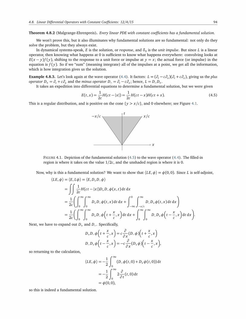
4.8. Linear Differential Operators with Constant Coefficients: 12/4/15 94
Theorem 4.8.2 (Malgrange-Ehrenpreis). Every linear PDE with constant coefficients has a fundamental solution.
We won’t prove this, but it also illuminates why fundamental solutions are so fundamental: not only do theysolve the problem, but they always exist.
In dynamical systems-speak, E is the solution, or response, and δ0 is the unit impulse. But since L is a linearoperator, then knowing what happens at 0 is sufficient to know what happens everywhere: convolving looks atE(x − y) f (y), shifting to the response to a unit force or impulse at y = x; the actual force (or impulse) in theequation is f (y). So if we “sum” (meaning integrate) all of the impulses at a point, we get all the information,which is how integration gives us the solution.
Example 4.8.3. Let’s look again at the wave operator (4.4). It factors: L = (∂t − c∂x )(∂t + c∂x ), giving us the plusoperator D+ = ∂t + c∂x and the minus operator D− = ∂t − c∂x ; hence, L = D−D+.
It takes an expedition into differential equations to determine a fundamental solution, but we were given
E(t, x) =12c
H(c t − |x |) =12c
H(c t − x)H(c t + x). (4.5)
This is a regular distribution, and is positive on the cone y > x/c, and 0 elsewhere; see Figure 4.1.
x
tx/c−x/c
FIGURE 4.1. Depiction of the fundamental solution (4.5) to the wave operator (4.4). The filled-inregion is where it takes on the value 1/2c, and the unshaded region is where it is 0.
Now, why is this a fundamental solution? We want to show that ⟨LE,φ⟩= φ(0,0). Since L is self-adjoint,
⟨LE,φ⟩= ⟨E, Lφ⟩= ⟨E, D+D−φ⟩
=
∫∫
12c
H(c t − |x |)D+D−φ(x , t)dt dx
=12c
∫ ∞
0
∫ ∞
0
D+D−φ(t, x)dt dx +
∫ 0
−∞
∫ ∞
−x/c
D−D+φ(t, x)dt dx
=12c
∫ ∞
0
∫ ∞
0
D+D−φ
t +xc
, x
dt dx +
∫ ∞
0
∫ ∞
0
D−D+φ
t −xc
, x
dt dx
.
Next, we have to expand out D+ and D−. Specifically,
D+D−φ
t +xc
, x
= c∂
∂ x(D−φ)
t +xc
, x
D−D+φ
t −xc
, x
= −c∂
∂ x(D+φ)
t −xc
, x
,
so returning to the calculation,
⟨LE,φ⟩= −12
∫ ∞
0
(D−φ(t, 0) + D+φ(t, 0))dt
= −12
∫ ∞
0
2∂
∂ t(t, 0)dt
= φ(0, 0),
so this is indeed a fundamental solution.
95 Chapter 4. Distributions
More generally, if Lu= f , then
u= E ∗ f =12c
∫ t
−∞
∫ x+c(t+s)
x−c(t−s)f (s, y)dy ds.
This equation implies some interesting physical properties of waves. Most notably, any point x at time 0 can onlyinfluence things in an expanding cone as time increases, called its domain of influence,10 which ultimately followsfrom the cone shape in Figure 4.1. Conversely, any point (x , t) can only be affected by points in an expandingcone as we go further into the past; this is its domain of dependence.
Example 4.8.4. Probably the most important example in applied mathematics is the Laplace operator or Laplacian
∆=∂ 2
∂ x21
+∂ 2
∂ x22
+ · · ·+∂ 2
∂ x2n
.
This is also written ∆=∇ ·∇=∇2. This shows up in many things, and is usually best thought of as a diffusionoperator. It’s also true but not obvious that it’s coordinate-independent.
Our fundamental solution will be given by
E(x) =
12|x |, d = 1
12π
ln|x |, d = 2
1dωd
|x |2−d
2− d, d > 2,
(4.6)
where ωd denotes the volume of the d-dimensional unit sphere (so cases d = 1 and d = 2 actually follow the samepattern as the general case).
For d = 1, this is easy to check, so let’s worry about the general case.E is actually in L1
loc; since the only singularity is at 0, we need to calculate the integral there, and we’ll do sowith polar coordinates for d = 2. If ε > 0,
∫
Bε(0)
12π
ln|x |
dx = 2π
∫ ε
0
12π
ln s
s ds =12
s2 ln s−s2
2
ε
0
,
which is finite. For general d > 2, we can ignore the constant terms, so using d-dimensional spherical coordinates,∫
Bε(0)
dx
|x |d−2=
∫ ε
0
1rd−2
rd−1C dr = C
∫ ε
0
r dr
for some constant C; thus, this is finite as well.Now, we need to show that E is indeed a fundamental solution. Here we need to use the divergence theorem.
Theorem 4.8.5 (Divergence). If Ω is a submanifold of Rd and φ and ψ are smooth functions on Ω, then∫
Ω
∇φ ·ψ=∫
∂Ω
φψ · ν−∫
Ω
φ∇ ·ψ,
where ν denotes the outward-pointing unit normal vector on the boundary ∂Ω.
Now, back to the calculation.
⟨∆E,φ⟩= ⟨E,∆φ⟩=∫
E(x)∆φ(x)dx .
10Yes, this is the positive lightcone in physics!
4.8. Linear Differential Operators with Constant Coefficients: 12/4/15 96
Now, we use the divergence theorem and the fact that∆φ =∇·(∇φ). Let ε > 0 and R be such that supp(φ) ( BR(0),so that
=
∫
ε<|x |<R
E∆φ +
∫
|x |<εE∆φ −
∫
ε<|x |<R
∇E · ∇φ +∫
|x |<εE∇φ · ν
=
∫
ε<|x |<R
∆E −∫
|x |=εφ∇E · ν+
∫
|x |=εE∇φ · ν.
You can directly calculate that ∆E = 0, so let’s attack the remaining two parts. Since ∇φ · ν doesn’t blow up asε→ 0, since φ is smooth, then
∫
|x |=εE∇φ · ν=
∫
S1(0)
1dωd
ε2−d
2− d∇φ · νεd−1 dσ = O(ε) −→ 0
as ε→ 0. The last part is
−∫
|x |=ε∇E · νφ dσ =
∫
S1(0)
∂ E∂ rφεd−1 dσ
=
∫
S1(0)
1dωd
|ε|1−dφ(ε,σ)εd−1 dσ −→ φ(0),
since φ is smooth.Notice that since E is supported everywhere, then the domain of dependence of diffusion is everywhere: the
speed of propgation is infinite, because things infinitely far away can affect you at arbitrarily small times. Thisseems a little odd — and so for some other kinds of diffusion, it may be necessary to use a more complicatedmodel (e.g. a nonlinear one). Nonetheless, because E tails off pretty quickly, local influences have a much strongereffect than global ones. Infinite propagation speed also causes all sorts of headaches numerically.
With a bit more work, one can extend this to L1, subject to a small condition.
Theorem 4.8.6. Let E be the fundamental solution to the Laplacian given in (4.6). Then, if f ∈ L1(Rd) andE(x − y) f (y) ∈ L1(Rd). Then, u= E ∗ f is a solution to ∆u= f in D ′.