M. Sc. MATHEMATICS

MAL-521

(ADVANCE ABSTRACT ALGEBRA)

Lesson No &Lesson Name Writer Vetter

1 Linear Transformations Dr. Pankaj Kumar Dr. Nawneet Hooda

2 Canonical Transformations Dr. Pankaj Kumar Dr. Nawneet Hooda

3 Modules I Dr. Pankaj Kumar Dr. Nawneet Hooda

4 Modules II Dr. Pankaj Kumar Dr. Nawneet Hooda

DIRECTORATE OF DISTANCE EDUCATIONS

GURU JAMBHESHWAR UNIVERSITY OF SCIENCE & TECHNOLOGY

HISAR 125001

MAL-521: M. Sc. Mathematics (Algebra)

Lesson No. 1 Written by Dr. Pankaj Kumar

Lesson: Linear Transformations Vetted by Dr. Nawneet Hooda

STRUCTURE

1.0 OBJECTIVE

1.1 INTRODUCTION

1.2 LINEAR TRANSFORMATIONS

1.3 ALGEBRA OF LINEAR TRANSFORMATIONS

1.4 CHARACTERISTIC ROOTS

1.5 CHARACTERISTIC VECTORS

1.6 MATRIX OF TRANSFORMATION

1.7 SIMILAR TRANSFORMATIONS

1.8 CANONICAL FORM(TRIANGULAR FORM)

1.9 KEY WORDS

1.10 SUMMARY

1.11 SELF ASSESMENT QUESTIONS

1.12 SUGGESTED READINGS

1.0 OBJECTIVE

Objective of this Chapter is to study Linear Transformation on the

finite dimensional vector space V over the field F.

1.1 INTRODUCTION

Let U and V be two given finite dimensional vector spaces over the

same field F. Our interest is to find a relation (generally called as linear

transformation) between the elements of U and V which satisfies certain

conditions and, how this relation from U to V becomes a vector space over the

field F. The set of all transformation on U into itself is of much interest. On

finite dimensional vector space V over F, for given basis of V, there always

exist a matrix and for given basis and given matrix of order n there always

exist a linear transformation.

In this Chapter, in Section 1.2, we study about linear transformations.

In Section 1.3, Algebra of linear transformations is studied. In next two

sections characteristic roots and characteristic vectors of linear transformations

are studied. In Section 1.6, matrix of transformation is studied. In Section 1.7

canonical transformations are studied and in last section we come to know

about canonical form (Triangular form).

1.2 LINEAR TRANSFORMATIONS

1.2.1 Definition. Vector Space. Let F be a field. A non empty set V with two

binary operations, addition (+)and scalar multiplications(.), is called a vector

space over F if V is an abelian group under + and for Vv∈ , Vv. ∈α . The

following conditions are also satisfied:

(1) α. (v+w) = αv+ αw for all F∈α and v, w in V,

(2) )( β+α .v = αv+β v,

(3) )(αβ .v = βα.( v)

(4) 1.v = v

For all α , β ∈ F and v, w belonging to V. Here v and w are called vectors and

α , β are called scalar.

1.2.2 Definition. Homomorphism. Let V and W are two vector space over the

same field F then the mapping T from V into W is called homomorphism if

(i) (v1+v2)T= v1T+v2 T

(ii) (αv1)T= α(v1T)

for all v1, v2 belonging to V and α belonging to F.

Above two conditions are equivalent to (αv1+βv2)T=α(v1T)+ β(v2T).

If T is one-one and onto mapping from V to W, then T is called an

isomorphism and the two spaces are isomorphic. Set of all homomorphism

from V to W is denoted by Hom(V, W) or HomR(V, W)

1.2.3 Definition. Let S and T∈ Hom(V, W), then S+T and λS is defined as:

(i) v(S+T)= vS+vT and

(ii) v(λS)= λ(vS) for all v∈V and λ∈F

1.2.4 Problem. S+T and λS are elements of Hom(V, W) i.e. S+T and λS are

homomorphisms from V to W.

Proof. For (i) we have to show that

(αu+βv)(S+T)= α(u(S+T))+ β(v(S+T))

By Definition 1.2.3, (αu+βv)(S+T)=(αu+βv)S+(αu+βv)T. Since S and T are

linear transformations, therefore,

(αu+βv)(S+T)=α(uS)+β(vS)+α(uT)+β(vT)

=α((uS)+α(uT))+β((vS)+(vT))

Again by definition 1.2.3, we get that (αu+βv)(S+T)=α(u(S+T))+β(v(S+T)). It

proves the result.

(ii) Similarly we can show that (αu+βv)(λS)=α(u(λS))+β(v(λS)) i.e. λS is also

linear transformation.

1.2.5 Theorem. Prove that Hom(V, W) becomes a vector space under the two

operation operations v(S+T)= vS + vT and v(λS)= λ(vS) for all v∈V, λ∈F

and S, T ∈Hom(V, W).

Proof. As it is clear that both operations are binary operations on Hom(V, W).

We will show that under +, Hom(V,W) becomes an abelian group. As

0∈Hom(V,W) such that v0=0 ∀ v∈V(it is call zero transformation), therefore,

v(S+0)= vS+v0 = vS = 0+vS= v0+vS= v(0+S) ∀ v∈V i.e. identity element

exists in Hom(V, W). Further for S∈Hom(V, W), there exist -S∈Hom(V, W)

such that v(S+(-S))= vS+v(-S)= vS-vS=0= v0 ∀ v∈V i.e. S+(-S)=0. Hence

inverse of every element exist in Hom(V, W). It is easy to see that

T1+(T2+T3)= (T1+T2)+T3 and T1+T2= T2+T1 ∀ T1, T2, T3∈Hom(V, W). Hence

Hom(V, W) is an abelian group under +.

Further it is easy to see that for all S, T ∈Hom(V, W) and α, β∈F, we

have α(S+T)= αS+αT, (α+β)S= αS+βS, (αβ)S= α(βS) and 1.S=S. It proves

that Hom(V, W) is a vector space over F.

1.2.6 Theorem. If V and W are vector spaces over F of dimensions m and n

respectively, then Hom(V, W) is of dimension mn over F.

Proof. Since V and W are vector spaces over F of dimensions m and n

respectively, let v1, v2,…, vm be basis of V over F and w1, w2,…, wn be basis

of W over F. Since mm2211 v...vvv δ++δ+δ= where iδ ∈F are uniquely

determined for v∈V. Let us define Tij from V to W by

viTij= jiwδ i.e. viTkj=⎩⎨⎧

≠

=

kiif0

kiifw j . It is easy to see that Tij

∈Hom(V,W). Now we will show that mn elements Tij 1≤ i ≤ m and 1≤j≤n

form the basis for Hom(V, W). Take

inin2i2i1i1in1n112121111 T...TT...T...TT β++β+β++β++β+β +

…+ mnmn2m2m1m1m T...TT β++β+β =0

(Since a linear transformation on V can be determined completely if image of

every basis element of it is determined)

⇒ inin2i2i1i1in1n112121111i T...TT...T...TT(v β++β+β++β++β+β +

…+ mnmn2m2m1m1m T...TT β++β+β )=vi0=0

⇒ nin22i11i w...ww β++β+β =0 (∴viTkj=⎩⎨⎧

≠

=

kiif0

kiifw j )

But w1, w2, …, wn are linearly independent over F, therefore,

0... in2i1i =β==β=β . Ranging i in 1≤i ≤m, we get each 0ij =β . Hence Tij

are linearly independent over F. Now we claim that every element of

Hom(V,W) is linear combination of Tij over F. Let S ∈Hom(V,W) such that

nn12121111 w...wwSv α++α+α= ,

nin22i11ii w...wwSv α++α+α=

nmn22m11mm w...wwSv α++α+α= .

Take inin2i2i1i1in1n1121211110 T...TT...T...TTS α++α+α++α++α+α= +

mnmn2m2m1m1m T...TT α++α+α .Then

0iSv = inin2i2i1i1in1n112121111i T...TT...T...TT(v α++α+α++α++α+α

+ mnmn2m2m1m1m T...TT α++α+α )

= nin22i11i w...ww α++α+α = Svi .

Similarly we can see that 0iSv = Svi for every i, 1≤ i ≤ m.

Therefore, 0vS = vS ∀ v∈V. Hence S0=S. It shows that every element of

Hom(V,W) is a linear combination of Tij over F. It proves the result.

1.2.7 Corollary. If dimension of V over F is n, then dimension of Hom(V,V) over F

=n2 and dimension of Hom(V,F) is n over F.

1.2.8 Note. Hom(V, F) is called dual space and its elements are called linear

functional on V into F. Let v1, v2,…, vn be basis of V over F then n21 v̂...,,v̂,v̂

defined by ⎩⎨⎧

≠=

=jiif0jiif1

)v(v̂ ji are linear functionals on V which acts as

basis elements for V. If v is non zero element of V then choose v1=v, v2,…, vn

as the basis for V. Then there exist 01)v(v̂)v(v̂ 111 ≠== . In other words we

have shown that for given non zero vector v in V we have a linear

transformation f(say) such that f(v)≠0.

1.3 ALGEBRA OF LINEAR TRANSFORMATIONS

1.3.1 Definition. Algebra. An associative ring A which is a vector space over F

such that α(ab)= (αa)b= a(αb) for all a, b∈A and α∈F is called an algebra

over F.

1.3.2 Note. It is easy to see that set of all Hom(V, V) becomes an algebra under the

multiplication of S and T ∈Hom(V, V) defined as:

v(ST)= (vS)T for all v∈ V.

we will denote Hom(V, V)=A(V). If dimension of V over F i.e. dimFV=n, then

dimF A(V)=n2 over F.

1.3.3 Theorem. Let A be an algebra with unit element and dimFA=n, then every

element of A satisfies some polynomial of degree at most n. In particular if

dimFV=n, then every element of A(V) satisfies some polynomial of degree at

most n2.

Proof. Let e be the unit element of A. As dimFA=n, therefore, for a∈A, the

n+1 elements e, a, a2,…,an are all in A and are linearly dependent over F, i.e.

there exist β0, β1,…, βn in F , not all zero, such that β0e+β1a+…+ βn an=0 . But

then a satisfies a polynomial β0+β1x+…+ βnxn over F. It proves the result.

Since the dimFA(V)=n2, therefore, every element of A(V) satisfies some

polynomial of degree at most n2.

1.3.4 Definition. An element T∈A(V) is called right invertible if there exist

S∈A(V) such that TS=I. Similarly ST=I (Here I is identity mapping) implies

that T is left invertible. An element T is called invertible or regular if it both

right as well as left invertible. If T is not regular then it is called singular

transformation. It may be that an element of A(V) is right invertible but not

left. For example, Let F be the field of real numbers and V be the space of all

polynomial in x over F. Define T on V by dx

)x(dfT)x(f = and S by

∫=x

1dx)x(fS)x(f . Both S and T are linear transformations. Since

)x(f)ST)(x(f ≠ i.e. ST≠I and )x(f)TS)(x(f = i.e. TS =I. Here T is right

invertible while it is not left invertible.

1.3.5 Note. Since T∈A(V) satisfies some polynomial over F, the polynomial of

minimum degree satisfied by T is called the minimal polynomial of T over F

1.3.6 Theorem. If V is finite dimensional over F, then T∈A(V) is invertible if and

only if the constant term of the minimal polynomial for T is non zero.

Proof. Let p(x)= β0+β1x+…+ βnxn , 0n ≠β , be the minimal polynomial for T

over F. First suppose that 00 ≠β , then 0 = p(T)= β0+β1T+…+ βnTn implies

that -β0I=T(β1T+…+βnTn-1) or

1n

0

1

0

1

0

1 T...T(TI −ββ

−−−ββ

−ββ

−= ) T)T...T( 1n

0

1

0

1

0

1 −ββ

−−−ββ

−ββ

−= .

Therefore, )T...T(S 1n

0

1

0

1

0

1 −ββ

−−−ββ

−ββ

−= is the inverse of T.

Conversely suppose that T is invertible, yet 00 =β . Then β1T+…+

βnTn =0 ⇒ (β1T+…+ βnTn-1)T=0 . As T is invertible, on operating T-1 on both

sides of above equations we get (β1T+…+ βnTn-1)=0 i.e. T satisfies a

polynomial of degree less then the degree of minimal polynomial of T,

contradicting to our assumption that 00 =β . Hence 00 ≠β . It proves the

result.

1.3.7 Corollary. If V is finite dimensional over F and if T ∈A(V) is singular, then

there exist non zero element S of A(V) such that ST=TS=0.

Proof. Let p(x)= β0+β1x+…+ βnxn , 0n ≠β be the minimal polynomial for T

over F. Since T is singular, therefore, constant term of p(x) is zero. Hence

(β1T+…+ βnTn-1)T=T(β1T+…+ βnTn-1)=0. Choose S=(β1T+…+ βnTn-1), then

S≠0(if S=0, then T satisfies the polynomial of degree less than the degree of

minimal polynomial of it) fulfill the requirement of the result.

1.3.8 Corollary. If V is finite dimensional over F and if T belonging to A(V) is

right invertible, then it is left invertible also. In other words if T is right

invertible then it is invertible.

Proof. Let U∈A(V) be the right inverse of T i.e. TU=I. If possible suppose T

is singular, then there exist non-zero transformation S such that ST=TS=0.

As

S(TU)= (ST)U

⇒ SI=0U ⇒ S=0, a contradiction that S is non zero. This

contradiction proves that T is invertible.

1.3.9 Theorem. For a finite dimensional vector space over F, T∈A(V) is singular if

and only if there exist a v≠0 in V such that vT=0.

Proof. By Corollary 1.3.7, T is singular if and only if there exist non zero

element S∈A(V) such that ST=TS=0. As S is non zero, therefore, there exist

an element u∈V such that uS≠0. More over 0=u0=u(ST)=(uS)T. Choose

v=uS, then v≠0 and vT=0. It prove the result.

1.4 CHARACTERISTIC ROOTS

In rest of the results, V is always finite dimensional vector space over F.

1.4.1 Definition. For T∈A(V), λ∈F is called Characteristic root of T if λI-T is

singular where I is identity transformation in A(V).

If T is singular, then clearly 0 is characteristic root of T.

1.4.2 Theorem. The element λ∈F is called characteristic root of T if and only there

exist an element v≠0 in V such that vT=λv.

Proof. Since λ is characteristic root of T, therefore, by definition the mapping

λI-T is singular. But then by Theorem 1.3.9, λI-T is singular if and only if

v(λI-T)=0 for some v≠0 in V. As v(λI-T)=0⇒vλ-vT=0⇒ vT= λv. Hence λ∈F

is characteristic root of T if and only there exist an element v≠0 in V such that

vT=λv.

1.4.3 Theorem. If λ∈F is a characteristic root of T, then for any polynomial q(x)

over F[x], q(λ) is a characteristic root of q[T].

Proof. By Theorem 1.4.2, if λ∈F is characteristic root of T then there exist an

element v≠0 in V such that vT=λv. But then vT2=(vT)T=(λv)T=λλv= λ2v. i.e.

vT2=λ2v. Continuing in this way we get, vTk=λkv. Let q(x)=β0+β1x+…+ βnxn ,

then q(T)= β0+β1T+…+ βnTn . Now by above discussion,

vq(T)=v(β0+β1T+…+ βnTn )= β0v+β1(vT)+…+ βn (vTn)= β0v+β1 λ2v +…+ βn

λnv = (β0+β1 λ2 +…+ βn λn)v=q(λ)v. Hence q(λ) is characteristic root of q(T).

1.4.4 Theorem. If λ is characteristic root of T, then λ is a root of minimal

polynomial of T. In particular, T has a finite number of characteristic roots in

F.

Proof. As we know that if λ is a characteristic root of T, then for any

polynomial q(x) over F, there exist a non zero vector v such that vq(T)=q(λ)v.

If we take q(x) as minimal polynomial of T then q(T)=0. But then vq(T)=q(λ)v

⇒ q(λ)v=0. As v is non zero, therefore, q(λ)=0 i.e. λ is root of minimal

polynomial of T.

1.5 CHARACTERISTIC VECTORS

1.5.1 Definition. The non zero vector v∈V is called characteristic vector belonging

to characteristic root λ ∈F if vT=λv.

1.5.2 Theorem. If v1, v2,…,vn are different characteristic vectors belonging to

distinct characteristic roots λ1, λ2,…, λn respectively , then v1, v2,…,vk are

linearly independent over F.

Proof. Let if possible v1, v2,…,vn are linearly dependent over F, then there

exist a relation β1v1+…+ βnvn=0 , where β1,+…+ βn are all in F and not all of

them are zero. In all such relation, there is one relation having as few non zero

coefficient as possible. By suitably renumbering the vectors, let us assume that

this shortest relation be

β1v1+…+ βkvk=0, where β1≠0,…, βk≠0. (i)

Applying T on both sides and using viT=λivi in (i) we get

λ1 β1v1+…+ λk βkvk=0 (ii)

Multiplying (i) by λ1 and subtracting from (ii), we obtain

(λ2-λ1)β2v2+…+ (λk-λ1)βkvk=0

Now (λi-λ1)≠0 for i>1 and β2≠0, therefore, (λi-λ1)βi≠0. But then we obtain a

shorter relation than that in (i) between v1, v2,…,vn. This contradiction proves

the theorem.

1.5.3 Corollary. If dimFV=n, then T∈A(V) can have at most n distinct

characteristic roots in F.

Proof. Let if possible T has more than n distinct characteristic roots in F, then

there will be more than n distinct characteristic vectors belonging to these

distinct characteristic roots. By Theorem 1.5.2, these vectors will be linearly

independent over F. Since dimFV=n, these n+1 element will be linearly

dependent, a contradiction. This contradiction proves T can have at most n

distinct characteristic roots in F.

1.5.4 Corollary. If dimFV=n and T∈A(V) has n distinct characteristic roots in F.

Then there is a basis of V over F which consists of characteristic vectors of T.

Proof. As T has n distinct characteristic roots in F, therefore, n characteristic

vectors belonging to these characteristic roots will be linearly independent

over F. As we know that if dimFV=n then every set of n linearly independent

vectors acts as basis of V(prove it). Hence set of characteristic vectors will act

as basis of V over F. It proves the result.

Example. If T ∈A(V) and if q(x) ∈F[x] is such that q(T)=0, is it true that

every root of q(x) in F is a characteristic root of T? Either prove that this is

true or give an example to show that it is false.

Solution. It is not true always. For it take V, a vector space over F with

dimFV=2 with v1 and v2 as basis element. It is clear that for v∈V, we have

unique α, β in F such that v=αv1+βv2. Define a transformation T∈A(V) by

v1T=v2 and v2T=0. let λ be characteristic root of T in F, then λI-T is singular.

It mean there exist a vector v(≠0) in V such that

vT=λv ⇒ (αv1+βv2)T=λαv1+λβv2 ⇒ α(v1T)+β(v2T)=λαv1+λβv2 ⇒

αv2+β.0=λαv1+λβv2 . As v is nonzero vector, therefore, at least one of α or β

is nonzero. But then αv2+β.0=λαv1+λβv2 implies that λ=0. Hence zero is the

only characteristic root of T in F. If We take a polynomial q(x)=x2(x-1), then

q(T)=T2(T-I). Now v1q(T)= ((v1T)T)(T-I) =(v2T)(T-I)=0(T-I)=0, v2q(T)=

((v2T)T)(T-I) =(0T)(T-I)=0 , therefore, vq(T)=0 ∀ v∈V . Hence q(T)=0. As

every root of q(x) lies in F yet every root of T is not a characteristic root of T.

Example. If T∈A(V) and if p(x) ∈F[x] is the minimal polynomial for T over

F, suppose that p(x) has all its roots in F. Prove that every root of p(x) is a

characteristic root of T.

Solution. Let p(x)= xn + β1 xn-1 +…+β0be the minimal polynomial for T and λ

be its root. Then p(x)= (x-λ)(xn-1 + γ1xn-2 +…+γ0). Since p(T)=0, therefore,

(T-λ)(Tn-1 + γ1 Tn-2 +…+γ0)=0. If (T-λ) is regular then (Tn-1

+γ1 Tn-2 +…+γ0)=0,

contradicting the fact that the minimal polynomial of T is of degree n over F.

Hence (T-λ) is not regular i.e. (T-λ) is singular and hence there exist a non

zero vector v in V such that v(T-λ)=0 i.e. vT=λv. Consequently λ is

characteristic root of T.

1.6 MATRIX OF TRANSFORMATIONS

1.6.1 Notation. The matrix of T under given basis of V is denoted by m(T).

We know that for determining a transformation T∈A(V) it is sufficient to find

out the image of every basis element of V. Let v1, v2,…,vn be the basis of V

over F and let

nn12121111 v...vvTv α++α+α=

… … … … …

nin22i11ii v...vvTv α++α+α=

… … … … …

nnn22n11nn v...vvTv α++α+α=

Then matrix of T under this basis is

m(T)=

nnnn2n1n

in2i1i

n11211

...............

................

...

×⎥⎥⎥⎥⎥⎥

⎦

⎤

⎢⎢⎢⎢⎢⎢

⎣

⎡

ααα

ααα

ααα

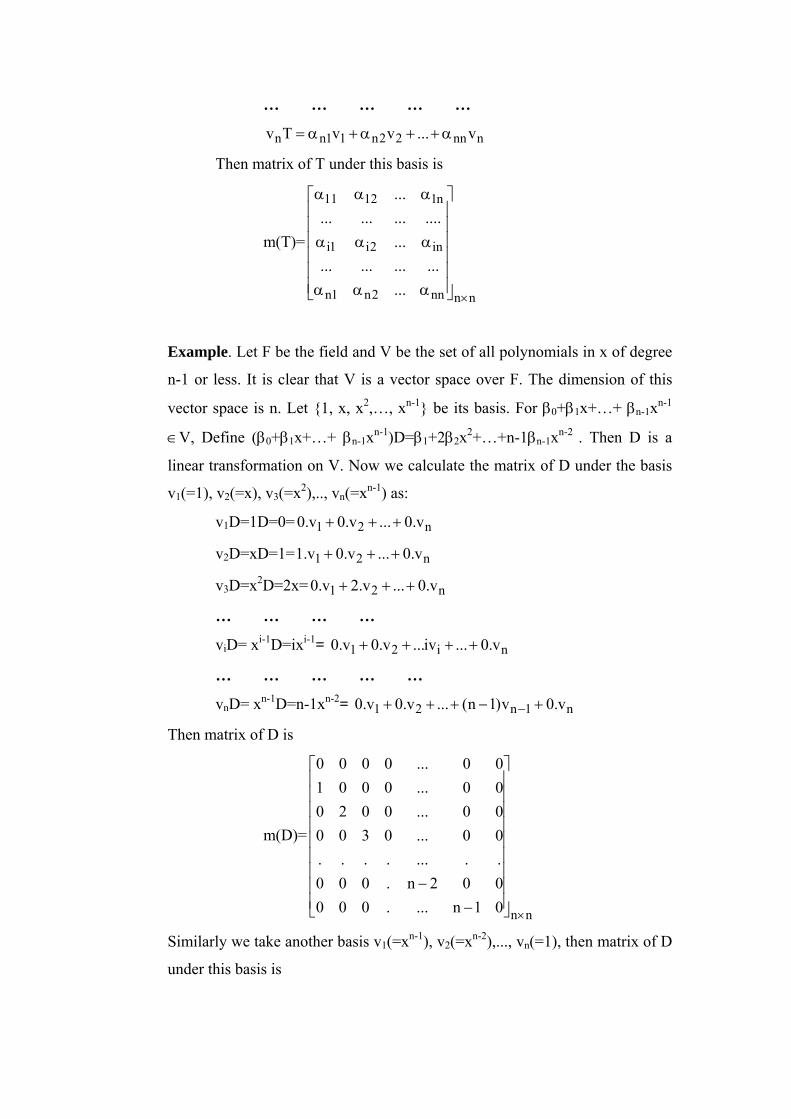
Example. Let F be the field and V be the set of all polynomials in x of degree

n-1 or less. It is clear that V is a vector space over F. The dimension of this

vector space is n. Let {1, x, x2,…, xn-1} be its basis. For β0+β1x+…+ βn-1xn-1

∈V, Define (β0+β1x+…+ βn-1xn-1)D=β1+2β2x2+…+n-1βn-1xn-2 . Then D is a

linear transformation on V. Now we calculate the matrix of D under the basis

v1(=1), v2(=x), v3(=x2),.., vn(=xn-1) as:

v1D=1D=0= n21 v.0...v.0v.0 +++

v2D=xD=1= n21 v.0...v.0v.1 +++

v3D=x2D=2x= n21 v.0...v.2v.0 +++

… … … …

viD= xi-1D=ixi-1= ni21 v.0...iv...v.0v.0 ++++

… … … … …

vnD= xn-1D=n-1xn-2= n1n21 v.0v)1n(...v.0v.0 +−+++ −

Then matrix of D is

m(D)=

nn01n....000002n.000.........00...030000...002000...000100...0000

×⎥⎥⎥⎥⎥⎥⎥⎥⎥

⎦

⎤

⎢⎢⎢⎢⎢⎢⎢⎢⎢

⎣

⎡

−−

Similarly we take another basis v1(=xn-1), v2(=xn-2),..., vn(=1), then matrix of D

under this basis is

m1(D)=

nn0.......00010......000

0...............000...3n00000...02n0000...001n0

×⎥⎥⎥⎥⎥⎥⎥⎥⎥

⎦

⎤

⎢⎢⎢⎢⎢⎢⎢⎢⎢

⎣

⎡

−−

−

MMMMMMM

If we take the basis v1(=1), v2(=1+x), v3(=1+x2),.., vn(=1+xn-1) then the matrix

of D under this basis is obtained as:

v1D=1D=0= n21 v.0...v.0v.0 +++

v2D=(1+x)D=1= n21 v.0...v.0v.1 +++

v3D=(1+x2)D=2x=-2+2(1+x)= n21 v.0...v.2v.2 +++−

… … … …

vnD=xn-1D=n-1xn-2=-(n-1)+n-1(1+xn-2)= n1n1 v.0v)1n(...v).1n( +−++−− −

Then matrix of D is

m3(D)=

nn01n....00)1n(002n.00)2n(.........00...030300...002200...000100...0000

×⎥⎥⎥⎥⎥⎥⎥⎥⎥

⎦

⎤

⎢⎢⎢⎢⎢⎢⎢⎢⎢

⎣

⎡

−−−−−−

−−

1.6.3 Theorem. If V is n dimensional over F and if T∈A(V) has a matrix m1(T) in

the basis v1, v2,…,vn and the matrix in the basis in the basis w1, w2,…,wn of V

over F. Then there is an element C∈Fn such that m2(T)= Cm1(T)C-1. In fact C

is matrix of transformation S∈A(V) where S is defined by viS=wi ; 1≤i ≤n.

Proof. Let m1(T)=(αij) , therefore, for 1≤i ≤n,

viT=αi1v1+αi2v2+…+αinvn= ∑=α

n

1jjijv (1)

Similarly, if m2(T)=(βij) , therefore, for 1≤i ≤n,

wiT=βi1w1+βi2w2+…+βinwn= ∑=β

n

1jjijw (2)

Since viS=wi , the mapping one –one and onto. Using viS=wi in (2) we get

viST=βi1(v1S)+βi2(v2S)+…+βin(vnS)

=(βi1.v1+βi2v2+…+βinvn)S

As S is invertible, therefore, on applying S-1 on both sides of above equation

we get vi (STS-1)=(βi1.v1+βi2v2+…+βinvn). Then by definition of matrix we

get m1(STS-1)=(βij)= m2(T). As the mapping T→m(T) is an isomorphism from

A(V) to Fn, therefore, m1(STS-1)= m1(S)m1(T)m1(S-1)= m1(S)m1(T)m1(S)-1 =

m2(T). Choose C= m1(S), then the result follows.

Example. Let V be the vector space of all polynomial of degree 3 or less over

the field of reals. Let T ∈A(V) is defined as: (β0+β1x+β2x2+β3x3)T

=β1+2β2x+3β3x2. Then D is a linear transformation on V. The matrix of T in

the basis v1(=1), v2(=x), v3(=x2), v4(=x3) as:

v1T=1T=0= 4321 v.0v0v.0v.0 +++

v2T=xT =1= 4321 v.0v0v.0v.1 +++

v3T=x2T=2x= 4321 v.0v0v.2v.0 +++

v4T= x3T=3x2= 4321 v.0v3v.0v.0 +++

Then matrix of t is

m1(D)=

⎥⎥⎥⎥

⎦

⎤

⎢⎢⎢⎢

⎣

⎡

0300002000010000

Similarly matrix of T in the basis w1(=1), w2(=1+x), w3(=1+x2), w4(=1+x3), is

m2(D)=

⎥⎥⎥⎥

⎦

⎤

⎢⎢⎢⎢

⎣

⎡

−−

0303002200010000

.

If We set viS=wi, then

v1S= w1= 1= 4321 v.0v0v.0v.1 +++

v2S=w2 = 1+x= 4321 v.0v0v.1v.1 +++

v3S=w3=1+x2 = 4321 v.0v1v.0v.1 +++

v4T= w4=1+x3= 4321 v.1v0v.0v.1 +++

But the C=m(S)=

⎥⎥⎥⎥

⎦

⎤

⎢⎢⎢⎢

⎣

⎡

1001010100110001

and C-1=

⎥⎥⎥⎥

⎦

⎤

⎢⎢⎢⎢

⎣

⎡

−−−

1001010100110001

and

Cm1(D)C-1=

⎥⎥⎥⎥

⎦

⎤

⎢⎢⎢⎢

⎣

⎡

1001010100110001

⎥⎥⎥⎥

⎦

⎤

⎢⎢⎢⎢

⎣

⎡

0300002000010000

⎥⎥⎥⎥

⎦

⎤

⎢⎢⎢⎢

⎣

⎡

−−−

1001010100110001

=

⎥⎥⎥⎥

⎦

⎤

⎢⎢⎢⎢

⎣

⎡

−−

0303002200010000

=m2(D) as required.

1.6.3 Note. In above example we see that for given basis of V there always exist a

square matrix of order equal to the dimFV. Converse part is also true. i.e. for

given basis and given matrix there always exist a linear transformation. Let V

be the vector space of all n-tuples over the field F, then Fn the set of all n×n

matrix is an algebra over F. In fact if v1=(1,0,0…,0), v2=(0,1,0…,0) ,…,

vn=(0,0,0…,n), then (αij)∈Fn acts as: v1(αij)= first row of (αij), …, vi(αij)= ith

row of (αij). We denote Mt is a square matrix of order t such that its each super

diagonal entry is one and the rest of the entries are zero. For example

M3 =

33000100010

×⎥⎥⎥

⎦

⎤

⎢⎢⎢

⎣

⎡ and M4 =

440000100001000010

×⎥⎥⎥⎥

⎦

⎤

⎢⎢⎢⎢

⎣

⎡

1.7 SIMILAR TRANSFORMATIONS.

1.7.1 Definition (Similar transformations). Transformations S and T belonging to

A(V) are said to similar if there exist R∈A(V) such that RSR-1=T.

1.7.2 Definition. A subspace W of vector space V is invariant under T∈A(V) if

WT⊆W. In other words wT ∈W ∀ w∈W.

1.7.3 Theorem. If subspace W of vector space is invariant under T, then T induces a

linear transformation T on WV , defined by WvTT)Wv( +=+ . Further if T

satisfies the polynomial q(x) over F, then so does T .

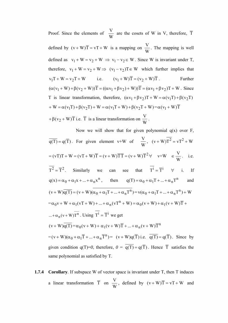
Proof. Since the elements of WV are the cosets of W in V, therefore, T

defined by WvTT)Wv( +=+ is a mapping on WV . The mapping is well

defined as WvWv 21 +=+ ⇒ Wvv 21 ∈− . Since W is invariant under T,

therefore, WvWv 21 +=+ ⇒ WT)vv( 21 ∈− which further implies that

WTvWTv 21 +=+ i.e. T)Wv(T)Wv( 21 +=+ . Further

WT)vv(T))W)vv((T))Wv()Wv(( 212121 +β+α=+β+α=+β++α . Since

T is linear transformation, therefore, )Tv()Tv(WT)vv( 2121 β+α=+β+α

)WTv()WTv(W)Tv()Tv(W 2121 +β++α=+β+α=+ = T)Wv( 1 +α

T)Wv( 2 +β+ i.e. T is a linear transformation on WV .

Now we will show that for given polynomial q(x) over F,

)T(q)T(q = . For given element v+W of WV , WvTT)Wv( 22 +=+

2T)Wv(TT)Wv(T)WvT(WT)vT( +=+=+=+= ∀ v+W ∈WV . i.e.

22 TT = . Similarly we can see that ii TT = ∀ i. If

nn10 x...x)x(q α++α+α= , then n

n10 T...T)T(q α++α+α= and

)T...T)(Wv()T(q)Wv( nn10 α++α+α+=+ = W)T...T(v n

n10 +α++α+α

= ++α++α=+α+++α++α T)Wv()Wv()WvT(...)WvT(Wv 10n

n10

nn T)Wv(... +α+ . Using ii TT = we get

)T(q)Wv( + = ++α )Wv(0n

n1 T)Wv(...T)Wv( +α+++α

= )T...T)(Wv( nn10 α++α+α+ = )T(q)Wv( + i.e. )T(q)T(q = . Since by

given condition q(T)=0, therefore, 0 = )T(q)T(q = . Hence T satisfies the

same polynomial as satisfied by T.

1.7.4 Corollary. If subspace W of vector space is invariant under T, then T induces

a linear transformation T on WV , defined by WvTT)Wv( +=+ and

minimal polynomial p1(x)(say) of T divides the minimal polynomial p(x) of

T.

Proof. Since p(x) is minimal polynomial of T, therefore, p(T)=0. But then by

Theorem 1.7.3, p( T )=0. Further, p1(x) is minimal polynomial of T , therefore,

p1(x) divides p(x).

1.8 CANONICAL FORM(TRIANGULAR FORM)

1.8.1 Definition. Let T be a linear transformation on V over F. The matrix of T in

the basis n21 v,...,v,v is called triangular if

1111 vTv α= ,

2221212 vvTv α+α=

… … …. …

iii22i11ii v...vvTv α+α+α=

…. … …. . ….

nnn22n11nn v...vvTv α+α+α=

1.8.2 Theorem. If T∈A(V) has all its characteristic roots in F, then there exist a

basis of V in which the matrix of T is triangular.

Proof. We will prove the result by induction on dimFV=n.

Let n=1. By Corollary 1.5.3, T has exactly one distinct root λ(say) in F. Let

v(≠0) be corresponding characteristic root in V. Then vT= λv. Since n=1. take

{v} as a basis of V. Now the matrix of T in this basis is [λ]. Hence the result is

true for n=1.

Choose n>1 and suppose that the result holds for all

transformations having all its roots in F and are defined on vector space V*

having dimension less then n.

Since T has all its characteristic roots in F; let λ1 be the root

characteristic roots in F and v1 be the corresponding characteristic vector.

Hence v1T=λ1v1. Choose W={αv1 | α∈F}. Then W is one dimensional

subspace of V. Since (αv1)T=α(v1 T)= αλ1v1 ∈W, therefore, W is invariant

under T. Let WVV̂ = . Then V̂ is a subspace of V such that dimF V̂ = dimFV-

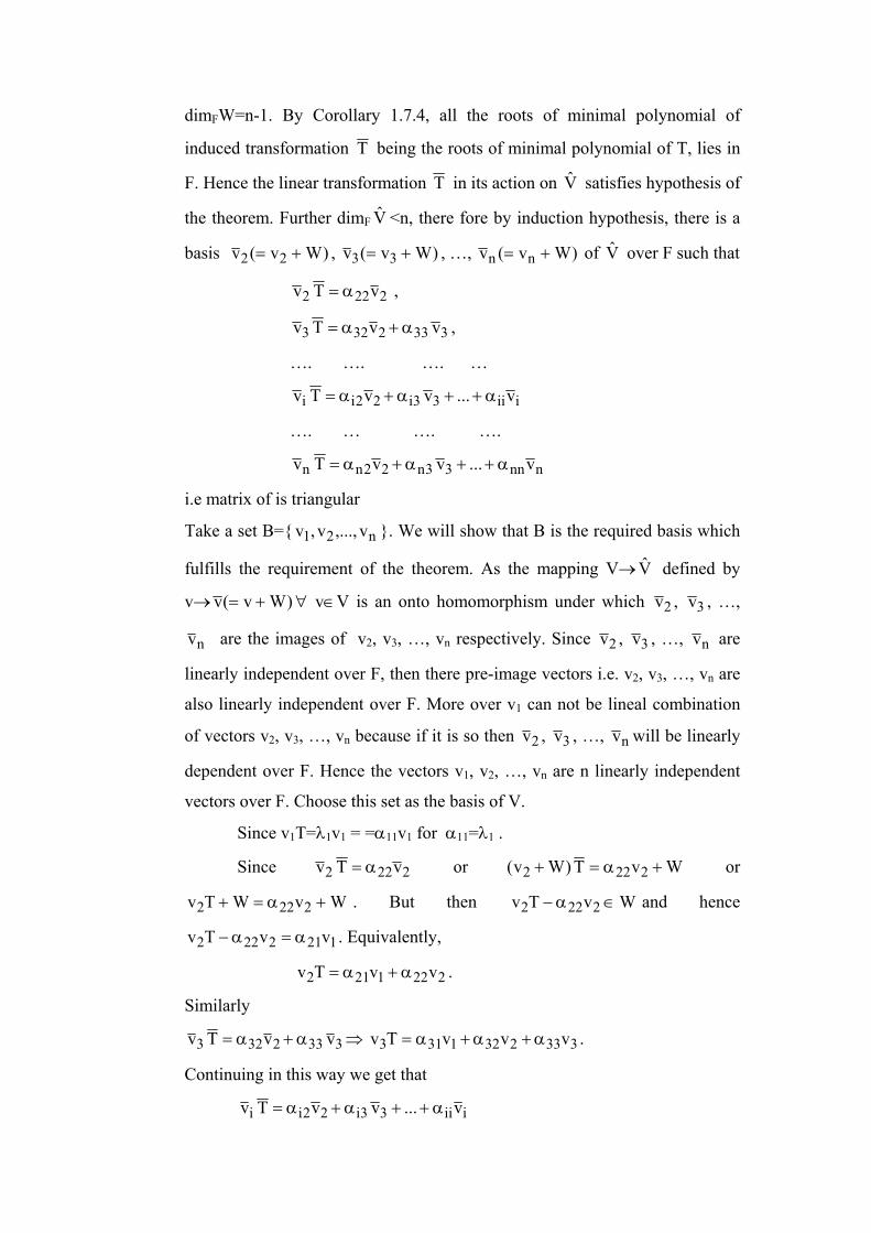
dimFW=n-1. By Corollary 1.7.4, all the roots of minimal polynomial of

induced transformation T being the roots of minimal polynomial of T, lies in

F. Hence the linear transformation T in its action on V̂ satisfies hypothesis of

the theorem. Further dimF V̂ <n, there fore by induction hypothesis, there is a

basis )Wv(v 22 += , )Wv(v 33 += , …, )Wv(v nn += of V̂ over F such that

2222 vTv α= ,

3332323 vvTv α+α= ,

…. …. …. …

iii33i22ii v...vvTv α++α+α=

…. … …. ….

nnn33n22nn v...vvTv α++α+α=

i.e matrix of is triangular

Take a set B={ n21 v,...,v,v }. We will show that B is the required basis which

fulfills the requirement of the theorem. As the mapping V→ V̂ defined by

v→ )Wv(v += ∀ v∈V is an onto homomorphism under which 2v , 3v , …,

nv are the images of v2, v3, …, vn respectively. Since 2v , 3v , …, nv are

linearly independent over F, then there pre-image vectors i.e. v2, v3, …, vn are

also linearly independent over F. More over v1 can not be lineal combination

of vectors v2, v3, …, vn because if it is so then 2v , 3v , …, nv will be linearly

dependent over F. Hence the vectors v1, v2, …, vn are n linearly independent

vectors over F. Choose this set as the basis of V.

Since v1T=λ1v1 = =α11v1 for α11=λ1 .

Since 2222 vTv α= or WvT)Wv( 2222 +α=+ or

WvWTv 2222 +α=+ . But then WvTv 2222 ∈α− and hence

1212222 vvTv α=α− . Equivalently,

2221212 vvTv α+α= .

Similarly

3332323 vvTv α+α= ⇒ 3332321313 vvvTv α+α+α= .

Continuing in this way we get that

iii33i22ii v...vvTv α++α+α=

⇒ iii22i11ii v...vvTv α++α+α= for all i, 1≤i≤n.

Hence B={v1, v2, …, vn} is the required basis in which the matrix of T is

triangular.

1.8.3 Theorem. If the matrix A∈Fn(=set of all n order square matrices over F) has

all its characteristic roots in F, then there is a matrix C∈Fn such that CAC-1 is

a triangular matrix.

Proof. Let A=[aij] ∈Fn. Further let Fn= {(α1, α2,…,αn)| αi∈F} be a vector

space over F and e1, e2,…, en be a basis of basis of V over F. Define T:V→V

by

niniii22i11ii ea...ea...eaeaTe +++++= .

Then T is a linear transformation on V and the matrix of T in this basis is

m1(T)= [aij]=A. Since the mapping A(V) →Fn defined by T→m1(T) is an

algebra isomorphism, therefore all the characteristic roots of A are in F.

Equivalently all the characteristic root of T are in F. Therefore, by Theorem

1.8.2, there exist a basis of V in which the matrix of T is triangular. Let it be

m2(T). By Theorem 1.6.3, there exist an invertible matrix C in Fn such that

m2(T)= Cm1(T)C-1= CAC-1 . Hence CAC-1 is triangular.

1.8.4 Theorem. If V is n dimensional vector space over F and let the matrix A∈Fn

has n distinct characteristic roots in F, then there is a matrix C∈Fn such that

CAC-1 is a diagonal matrix.

Proof. Since all the characteristic roots of matrix A are distinct, the linear

transformation T corresponding to this matrix under a given basis, also has

distinct characteristic roots say λ1, λ2,…, λn in F. Let v1, v2,…, vn be the

corresponding characteristic vectors in V . But then

ni1vTv iii ≤≤∀λ= (1)

We know that vectors corresponding to distinct characteristic root are linearly

independent over F. Since these are n linearly independent vectors over F and

dimension of V over F is n, therefore, set B={ v1, v2,…, vn } can be taken as

basis set of V over F. Now the matrix of T in this basis is

⎥⎥⎥⎥

⎦

⎤

⎢⎢⎢⎢

⎣

⎡

λ

λλ

n

2

1

...000......00...00...0

. Now By above Theorem, there

exist C in Fn such that CAC-1=

⎥⎥⎥⎥

⎦

⎤

⎢⎢⎢⎢

⎣

⎡

λ

λλ

n

2

1

...000......00...00...0

is diagonal matrix.

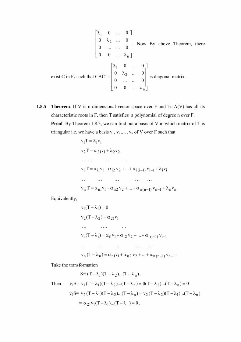
1.8.5 Theorem. If V is n dimensional vector space over F and T∈A(V) has all its

characteristic roots in F, then T satisfies a polynomial of degree n over F.

Proof. By Theorem 1.8.3, we can find out a basis of V in which matrix of T is

triangular i.e. we have a basis v1, v2,…, vn of V over F such that

111 vTv λ=

221212 vvTv λ+α=

… … … …

ii1i)1i(i22i11ii vv...vvTv λ+α++α+α= −−

… … … … …

nn1n)1n(n22n11nn vv...vvTv λ+α++α+α= −−

Equivalently,

0)T(v 11 =λ−

12122 v)T(v α=λ−

…. …. …

1i)1i(i22i11iii v...vv)T(v −−α++α+α=λ−

… … … … …

1n)1n(n22n11nnn v...vv)T(v −−α++α+α=λ− .

Take the transformation

S= )T)...(T)(T( n21 λ−λ−λ− .

Then v1S= 0)T)...(T(0)T)...(T)(T(v n2n211 =λ−λ−=λ−λ−λ−

v2S= )T)...(T)(T(v)T)...(T)(T(v n122n212 λ−λ−λ−=λ−λ−λ−

= 0)T)...(T(v n1121 =λ−λ−α .

Similarly we can see that viS=0 for 1≤ i ≤n. Equivalently, vS=0 ∀ v∈V. Hence

S= )T)...(T)(T( n21 λ−λ−λ− =0 i.e. S is zero transformation on V.

Consequently T satisfies the polynomial )x)...(x)(x( n21 λ−λ−λ− of degree

n over F.

1.9 KEY WORDS

Transformations, similar transformations, characteristic roots, canonical

forms.

1.10 SUMMARY

In this chapter, we study about linear transformations, Algebra of linear

transformations, characteristic roots and characteristic vectors of linear

transformations, matrix of transformation and canonical form (Triangular

form).

1.11 SELF ASSESMENT QUESTIONS

(1) If V is a finite dimensional vector space over the field of real numbers with

basis v1 and v2. Find the characteristic roots and corresponding characteristic

vectors for T defined by

(i) v1T = v1 + v2 , v2T = v1 - v2

(ii) v1T = 5v1 + 6v2 , v2T = -7v2

(iii) v1T = v1 + 2v2 , v2T = 3v1 + 6v2

(2) If V is two-dimensional vector space over F, prove that every element in

A(V) satisfies a polynomial of degree 2 over F

1.12 SUGGESTED READINGS:

(1) Topics in Algebra; I.N HERSTEIN, John wiley and sons, New York.

(2) Modern Algebra; SURJEET SINGH and QAZI ZAMEERUDDIN, Vikas

Publications.

(3) Basic Abstract Algebra; P.B. BHATTARAYA, S.K.JAIN, S.R.

NAGPAUL, Cambridge University Press, Second Edition.

MAL-521: M. Sc. Mathematics (Advance Abstract Algebra)

Lesson No. 2 Written by Dr. Pankaj Kumar

Lesson: Canonical forms Vetted by Dr. Nawneet Hooda

STRUCTURE

2.0 OBJECTIVE

2.1 INTRODUCTION

2.2 NILPOTENT TRANSFORMATION

2.3 CANONICAL FORM(JORDAN FORM)

2.4 CANONICAL FORM( RATIONAL FORM)

2.5 KEY WORDS

2.6 SUMMARY

2.7 SELF ASSESMENT QUESTIONS

2.8 SUGGESTED READINGS

2.0 OBJECTIVE

Objective of this Chapter is to study Nilpotent Transformations and

canonical forms of some transformations on the finite dimensional vector

space V over the field F.

2.1 INTRODUCTION

Let T ∈A(V), V is finite dimensional vector space over F. In first

chapter, we see that every T satisfies some minimal polynomial over F. If T is

nilpotent transformation on V, then all the characteristic root of T lies in F.

Therefore, there exists a basis of V under which matrix of T has nice form.

Some time all the root of minimal polynomial of T does not lies in F. In that

case we study, rational canonical form of T.

In this Chapter, in Section 2.2, we study about Nilpotent

transformations. In next Section, Jordan forms of a transformation are studied.

At the end of this chapter, we study, rational canonical forms.

2.2 NILPOTENT TRANSFORMATION

2.2.1 Definiton. Nilpotent transformation. A transformation T∈A(V) is called

nilpotent if Tn=0 for some positive integer n. Further if 0Tr = and 0Tk ≠

for k<r, then T is nilpotent transformation with index of nilpotence r.

2.2.2 Theorem. Prove that all the characteristic roots of a nilpotent transformation T

∈A(V) lies in F.

Proof. Since T is nilpotent, let r be the index of nilpotence of T. Then Tr=0 .

Let λ be the characteristic root of T, then there exist v(≠0) in V such that

vT=λv. As vT2=(vT)T= (λv)T=λ(vT)= λλv =λ2v . Therefore, continuing in

this way we get vT3=λ3v ,…, vTr=λrv . Since Tr=0 , hence vTr=v0 =0 and

hence λrv=0. But v≠0, therefore, λr=0 and hence λ=0, which all lies in F.

2.2.3 Theorem. If T∈A(V) is nilpotent and 00 ≠β , then β0+β1T+…+ βmTm ; Fi ∈β

is invertible.

Proof. If S is nilpotent then Sr=0 for some integer r. Let 00 ≠β , then

)S)1(...SSI)(S( r0

1r1r

30

2

200

0β

−++β

+β

−β

+β−

−

= r0

r1r

1r0

1r1r

1r0

1r1r

20

2

20

2

00

S)1(S)1(S)1(...SSSSIβ

−+β

−−β

−++β

+β

−β

+β

− −−

−−

−

−−

= I. Hence )S( 0 +β is invertible.

Now if Tk=0, then for the transformation

S=β1T+…+ βmTm,

vSk=v(β1T+…+ βmTm)k=vTk(β1+…+ βmTm-1)k ∀ v∈V.

Since Tk=0, therefore, vTk=0 and hence vSk=0 ∀ v∈V i.e. Sk=0. Equivalently,

Sk is a nilpotent transformation. But then by above discussion

β0+S=β0+β1T+…+ βmTm is invertible if 00 ≠β . It proves the result.

2.2.4 Theorem. If V= V1⊕V2⊕…⊕Vk where each subspace Vi of V is of dimension

ni and is invariant under T∈A(V). Then a basis of V can be found so that the

matrix of T in this basis is of the form

⎥⎥⎥⎥⎥⎥

⎦

⎤

⎢⎢⎢⎢⎢⎢

⎣

⎡

k

3

2

1

A000

0A0000A0000A

K

MMMM

K

K

K

where each

Ai is an ni×ni matrix and is the matrix of linear transformation iT induced by T

on Vi.

Proof. Since each Vi is of dimension ni, let { )1(n

)1(2

)1(1 1

v...,,v,v },

{ )2(n

)2(2

)2(1 2

v...,,v,v },…, { )i(n

)i(2

)i(1 i

v...,,v,v },…,{ )k(n

)k(2

)k(1 k

v...,,v,v } are the basis

of V1 , V2 ,…, Vi,…, Vk respectively, over F. We will show that

{ )1(n

)1(2

)1(1 1

v...,,v,v , )2(n

)2(2

)2(1 2

v...,,v,v ,…, )i(n

)i(2

)i(1 i

v...,,v,v ,…, )k(n

)k(2

)k(1 k

v...,,v,v }

is the basis of V. First we will show that these vectors are linearly independent

over F. Let

44444 844444 76)1(

n)1(

n)1(

2)1(

2)1(

1)1(

1 11v...vv α++α+α +

444444 8444444 76)2(

n)2(

n)2(

2)2(

2)2(

1)2(

1 22v...vv α++α+α +…+

44444 844444 76)i(

n)i(

n)i(

2)i(

2)i(

1)i(

1 iiv...vv α++α+α +…+

444444 8444444 76)k(

n)k(

n)k(

2)k(

2)k(

1)k(

1 kkv...vv α++α+α =0.

But V is direct sum of Vi’s therefore, zero has unique representation i.e.

0=0+0+…+0+…0. Hence 44444 844444 76

)i(n

)i(n

)i(2

)i(2

)i(1

)i(1 ii

v...vv α++α+α =0 for 1≤ i≤k. But

for 1≤ i≤k , )i(n

)i(2

)i(1 i

v...,,v,v are linearly independent over F. Hence

0... )i(n

)i(2

)i(1 i

=α==α=α and hence )1(n

)1(2

)1(1 1

v...,,v,v , )2(n

)2(2

)2(1 2

v...,,v,v ,…,

)i(n

)i(2

)i(1 i

v...,,v,v , …, )k(n

)k(2

)k(1 k

v...,,v,v are linearly independent over F. More

over for v∈V, there exist vi ∈Vi such that v=v1 + v2+…+vi +…+vk . But for 1≤

i ≤ k, F,nt1for;v...vvv )i(jii

)i(n

)i(n

)i(2

)i(2

)i(1

)i(1i ii

∈α≤≤α++α+α= . Hence

v= )k(n

)k(n

)k(1

)k(1

)1(n

)1(n

)1(1

)1(1 kk11

v...v...v...v α++α++α++α . In other words we can

say that every element of V is linear combination of )1(n

)1(2

)1(1 1

v...,,v,v ,

)2(n

)2(2

)2(1 2

v...,,v,v ,…, )i(n

)i(2

)i(1 i

v...,,v,v , …, )k(n

)k(2

)k(1 k

v...,,v,v over F. Hence

{ )1(n

)1(1 1

v...,,v , )2(n

)2(2

)2(1 2

v...,,v,v ,…, )i(n

)i(2

)i(1 i

v...,,v,v , …, )k(n

)k(2

)k(1 k

v...,,v,v } is

a basis for V over F. Define Ti on Vi by setting viTi=viT ∀ vi∈Vi. Then Ti is a

linear transformation on Vi. Since Vi are linealy independent, therefore, For

obtaining m(T) we proceed as:

=Tv )1(1

)1(n

)1(n1

)1(1

)1(12

)1(1

)1(11 11

v...vv α+α+α

=44444 844444 76

)1(n

)1(n1

)1(1

)1(12

)1(1

)1(11 11

v...vv α+α+α + )2(n

)2(1 2

v.0...v.0 ++ + )k(n

)k(1 k

v.0...v.0 ++ .

=Tv )1(2

)1(n

)1(n2

)1(1

)1(22

)1(1

)1(21 11

v...vv α+α+α

=44444 844444 76

)1(n

)1(n2

)1(1

)1(22

)1(1

)1(21 11

v...vv α+α+α + )2(n

)2(1 2

v.0...v.0 ++ + )k(n

)k(1 k

v.0...v.0 ++ .

… … … ….. …

=Tv )1(n1

)1(n

)1(nn

)1(1

)1(2n

)1(1

)1(1n 11111

v...vv α+α+α

=444444 8444444 76

)1(n

)1(nn

)1(1

)1(2n

)1(1

)1(1n 11111

v...vv α+α+α + )2(n

)2(1 2

v.0...v.0 ++ + )k(n

)k(1 k

v.0...v.0 ++ .

Since it is easy to see that m(T1)= 11 nn

)1(ij ][ ×α =A1. Therefore, role of T on V1

produces a part of m(T) given by [A1 0], here 0 is a zero matrix of order n1×n-

n1. Similarly part of m(T) obtained by the roll of T on V2 is [0 A2 0], here first

0 is a zero matrix of order n1×n1 , A2= 22 nn)2(

ij ][ ×α and the last zero is a zero

matrix of order n1×n-n1-n2. Continuing in this way we get that

⎥⎥⎥⎥⎥⎥

⎦

⎤

⎢⎢⎢⎢⎢⎢

⎣

⎡

k

3

2

1

A000

0A0000A0000A

K

MMMM

K

K

K

as required.

2.2.5 Theorem. If T∈A(V) is nilpotent with index of nilpotence n1, then there

always exists subspaces V1 and W invariant under T so that V =V1⊕W.

Proof. For proving the theorem, first we prove some lemmas:

Lemma 1. If T∈A(V) is nilpotent with index of nilpotence n1, then there

always exists subspace V1 of V of dimension n1 which is invariant under T.

Proof. Since index of nilpotence of T is n1 , therefore, 0T 1n = and 0Tk ≠ for

1≤ k ≤n1-1. Let v(≠0)∈V. Consider the elements v, vT, vT2, … 1n1vT − of V.

Take 0vT...vT...vTv 1nn

)1s(s21

11

=α++α++α+α−− , Fi ∈α and let sα be

the first non zero element in above equation. Hence

0vT...vT 1nn

)1s(s

11

=α++α−− . But then 0)T...(vT sn

ns)1s( 1

1=α++α

−− . As

0s ≠α and T is nilpotent, therefore, )T...( snns

11

−α++α is invertible and

hence Vv0vT )1s( ∈∀=− i.e. )1s(T − =0 for some integer less than n1, a

contradiction. Hence each 0i =α . It means elements v, vT, vT2,…, 1n1vT − are

linearly independent over F. Let V1 be the space generated by the elements v,

vT, vT2, …, 1n1vT − . Then the dimension of V1 over F is n1. Let u∈V1, then

u= 1nn

2n1n1

11

11

vTvT...v −−− β+β++β and

uT= 11

11

nn

1n1n1 vTvT...v β+β++β

−− = 1n

1n11

1vT...v −

−β++β

i.e. uT is also a linear combination of v, vT, vT2, …, 1n1vT − over F. Hence

uT∈V1. i.e. V1 is invariant under T.

Lemma(2). If V1 is subspace of V spanned by v, vT, vT2, …, 1n1vT − , T∈A(V)

is nilpotent with index of nilptence n1 and u∈V1 is such that 0uT kn1 =− ; 0 <

k ≤ n1, then u= k0Tu for some u0∈V1.

Proof. For u∈V1, u= 1nn

k1k

)1k(k1

11vT...vTvT...v −

+− α+α+α++α ; Fi ∈α .

and0= kn1uT − =( 1nn

k1k

)1k(k1

11vT...vTvT...v −

+− α+α+α++α ) kn1T −

= 1kn2n

n1k

1nk

kn1

11

111 vT...vTvT...vT −−+

−−α+α+α++α

= 1nk

kn1

11 vT...vT −−α++α . Since 1nkn 11 vT...vT −−

++ are

linearly independent over F, therefore, 0... k1 =α==α . But then

u= kknn1k

1nn

k1k T)vT...v(vT...vT 1

11

1−

+−

+ α++α=α++α . Put

.uvT...v 0kn

n1k1

1=α++α

−+ Then u=u0Tk. It proves the lemma.

Proof of Theorem. Since T is nilpotent with index of nilpotence n1, then by

Lemma 3, there always exist a subspace V1 of V generated by v, vT, vT2,…,

1n1vT − . Let W be the subspace of V of maximal dimension such that

(i) V1∩W=(0) and (ii) W is invariant under T.

We will show that V=V1+W. Let if possible V≠V1+W. then there exist z∈V

such that z∉V1+W. Since 1nT =0, therefore, 0zT 1n= . But then there exist an

integer 0 < k ≤n1 such that WVzT 1k +∈ and WVzT 1

i +∉ for 0<i<k. Let

wuzTk += . Since 1nzT0 = = knknkknk 111 T)wu(T)zT()TT(z −−− +== =

knkn 11 wTuT −− + , therefore, knkn 11 wTuT −− −= . But then 1kn VuT 1 ∈− and

W. Hence 0uT kn1 =− . By Lemma 3, u= k0Tu for some u0∈V1. Hence

wTuzT k0

k += or WT)uz( k0 ∈− . Take z1=z-u0, then WTz k

1 ∈ . Further,

for i<k, WTz i1 ∉ because if WTz i

1 ∈ , then .WTuzT i0

i ∈− Equivalently,

WVzT 1i +∈ , a contradiction to our earlier assumption that i<k,

.WVzT 1i +∉

Let W1 be the subspace generated by W, z1, z1T, z1T2,…,

1k1Tz − . Since z1 does not belongs to W, therefore, W is properly contained in

W1 and hence dimFW1> dimFW. Since W is invariant under T, therefore, W1 is

also invariant under T. Now by induction hypothesis, V1∩W1≠(0). Let

1k1k1211 Tz...Tzzw −α++α+α+ be a non zero element belonging to V1∩W1.

Here all iα ’s are not zero because then V1∩W≠(0). Let sα be the first non

zero iα . Then

1sk

ks1s

11k

1k1s

1s V)T...(TzwTz...Tzw ∈α++α+=α++α+ −−−− .

Since 0s ≠α , therefore , )T...(R skks

−α++α= is invertible and hence

11

11s

11 VRVTzwR ⊆∈+ −−− . Equivalently, WVTz 1

1s1 +∈− , a contradiction.

This contradiction proves that V=V1+W. Hence V=V1⊕W.

2.2.6 Theorem. If T∈A(V) is nilpotent with index of nilpotence n1, then there exist

subspace V1, V2, …, Vr, of dimensions n1, n2,…,nr respectively, each Vi is

invariant under T such that V= V1⊕V2⊕…⊕Vr , n1≥ n2 ≥…≥nr and dim V =

n1+n2+…+nr. More over we can find a basis of V over F in which matrix of T

is of the form

⎥⎥⎥⎥⎥⎥

⎦

⎤

⎢⎢⎢⎢⎢⎢

⎣

⎡

rn

3n

2n

1n

M000

0M0000M0000M

K

MMMM

K

K

K

.

Proof. First we prove a lemma. If T∈A(V) is nilpotent with index of

nilpotence n1 , V1 is a subspace of V spanned by v, vT, vT2, …, 1n1vT − where

v∈V. Then 1nM will be the matrix of T on V1 under the basis vv1 = ,

vTv2 = , …, 1nn 1

1vTv −= .

Proof. Since

=Tv1 0.v1+1.v2+…+0. 1nv

v2T=(vT)T=vT2= v3= 0.v1+0.v2+1.v3+…+0. 1nv

… … … …

11

11n21n1 n21n1n v.1...v.0v.0vvTT)vT(Tv +++==== −−− and

1

1n11n1 n211n v.0...v.0v.00vTT)vT(Tv +++==== − , therefore,

the matrix of T under the basis v, vT, vT2, …, 1n1vT − is

11 nn00001000001000010

×⎥⎥⎥⎥⎥⎥

⎦

⎤

⎢⎢⎢⎢⎢⎢

⎣

⎡

K

MMM

K

K

K

= 1nM .

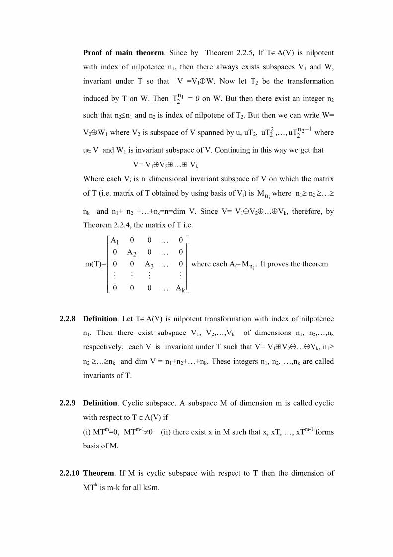
Proof of main theorem. Since by Theorem 2.2.5, If T∈A(V) is nilpotent

with index of nilpotence n1, then there always exists subspaces V1 and W,

invariant under T so that V =V1⊕W. Now let T2 be the transformation

induced by T on W. Then 1n2T = 0 on W. But then there exist an integer n2

such that n2≤n1 and n2 is index of nilpotene of T2. But then we can write W=

V2⊕W1 where V2 is subspace of V spanned by u, uT2, 22uT ,…, 1n

22uT − where

u∈V and W1 is invariant subspace of V. Continuing in this way we get that

V= V1⊕V2⊕…⊕ Vk

Where each Vi is ni dimensional invariant subspace of V on which the matrix

of T (i.e. matrix of T obtained by using basis of Vi) is inM where n1≥ n2 ≥…≥

nk and n1+ n2 +…+nk=n=dim V. Since V= V1⊕V2⊕…⊕Vk, therefore, by

Theorem 2.2.4, the matrix of T i.e.

m(T)=

⎥⎥⎥⎥⎥⎥

⎦

⎤

⎢⎢⎢⎢⎢⎢

⎣

⎡

k

3

2

1

A000

0A0000A0000A

K

MMMM

K

K

K

where each Ai= .Min It proves the theorem.

2.2.8 Definition. Let T∈A(V) is nilpotent transformation with index of nilpotence

n1. Then there exist subspace V1, V2,…,Vk of dimensions n1, n2,…,nk

respectively, each Vi is invariant under T such that V= V1⊕V2⊕…⊕Vk, n1≥

n2 ≥…≥nk and dim V = n1+n2+…+nk. These integers n1, n2, …,nk are called

invariants of T.

2.2.9 Definition. Cyclic subspace. A subspace M of dimension m is called cyclic

with respect to T ∈A(V) if

(i) MTm=0, MTm-1≠0 (ii) there exist x in M such that x, xT, …, xTm-1 forms

basis of M.

2.2.10 Theorem. If M is cyclic subspace with respect to T then the dimension of

MTk is m-k for all k≤m.

Proof. Since M is cyclic with respect to T, therefore, there exist x in M such

that x, xT, …, xTm-1 is a basis of M. But then z∈M,

z= a1x+ a2xT+ …+ am xTm-1; ai∈F

Equivalently, zTk= a1xTk+ a2xTk+1+ …+ am-kxTm-1 +..+am xTm+k= a1xTk+

a2xTk+1+ …+ am-kxTm-1. Hence every element z of MTk is linear combination

of m-k elements xTk, xTk+1, …,xTm-1 . Being a subset of linearly independent

set these are linearly independent also. Hence the dimension of MTk is m-k for

all k.

2.2.11 Theorem. Prove that invariants of a nilpotent transformation are unique.

Proof. Let if possible there are two sets of invariant n1, n2, …, nr and m1 , m2,

…, mr of T. Then V= V1⊕V2⊕…⊕ Vr and V= W1⊕W2⊕…⊕ Ws, where each

Vi and Wi’s are cyclic subspaces of V of dimension ni and mi respectively, We

will show that r=s and ni=mi. Suppose that k be the first integer such that

nk≠mk. i.e. n1=m1, n2=m2,…, nk-1=mk-1. Without loss of generality suppose that

nk>mk. Consider kmVT . Then

kkkk mr

m2

m1

m TV...TVTVVT ⊕⊕⊕= and

)TVdim(...)TVdim()TVdim()VTdim( kkkk mr

m2

m1

m +++= . As by Theorem

2.2.10, kim

i mn)TVdim( k −= , therefore,

)mn(...)mn()VTdim( k1kk1mk −++−≥ − (1)

Similarly )TWdim(...)TWdim()TWdim()VTdim( kkkk ms

m2

m1

m +++= . As

mj ≤ mk for j ≥ k, therefore, }0{TW kmj = subspace and then

0)TWdim( kmj = . Hence )mm(...)mm()VTdim( k1kk1

mk −++−≥ − . Since

n1=m1, n2=m2,…,nk-1 =mk-1, therefore,

)VTdim( km = )mn(...)mn( k1kk1 −++− − , contradicting (1). Hence ni=mi.

Further n1+n2+…+nr= dim V=m1+m2+…+ms and ni=mi for all i implies that

r=s. It proves the theorem.

2.2.12 Theorem. Prove that transformations S and T∈A(V) are similar iff they have

same invariants.

Proof. First suppose that S and T are similar i.e. there exist a regular mapping

R such that RTR-1=S. Let n1, n2,…, nr be the invariants of S and m1 , m2, …,

ms are that of T. Then V= V1⊕V2⊕…⊕ Vr and V= W1⊕W2⊕…⊕ Ws, where

each Vi and Wi’s are cyclic and invariant subspaces of V of dimension ni and

mi respectively, We will show that r=s and ni=mi.

As ViS ⊆Vi, therefore, Vi (RTR-1)⊆Vi ⇒ (ViR)(TR-1) ⊆ Vi. Put Vi R= Ui.

Since R is regular, therefore, dim Ui=dimVi=ni. Further UiT= Vi RT= Vi SR.

As ViS ⊆Vi, therefore, UiT⊆Ui. Equivalently we have shown that Ui is

invariant under T. More over

V=VR= V1R⊕V2R⊕…⊕ VrR=U1⊕U2⊕…⊕ Ur.

Now we will show that each Ui is cyclic with respect to T. Since each Vi is

cyclic with respect to S and is of dimension ni, therefore, for v∈Vi, v,

vS,…, 1nivS − is basis of Vi over F. As R is regular transformation on V,

therefore, vR, vSR,…, 1nivS − R is also a basis of V. Further S=RTR-1 ⇒

SR=RT ⇒ S2R=S(SR)=S(RT)=(SR)T=RTT= RT2. Similarly we have

StR=RTt. Hence {vR, vSR,…, 1nivS − R} = {vR, vRT,…, 1nivRT − }. Now vR

lies in Ui whose dimension is ni and vR, vRT,…, 1nivRT − are ni elements

linearly independent in Ui, the set {vR, vRT,…, 1nivRT − } becomes a basis of

Ui. Hence Ui is cyclic with respect to T. Hence invariant of T are n1, n2,…,nr .

As by Theorem 2.2.11, the invariants of nilpotents transformations are unique,

therefore, ni=mi and r=s.

Conversely, suppose that two nilpotent transformations R and S have

same invariants. We will show that they are similar. As they have same

invariants, therefore, there exist two basis say X={x1, x2,…, xn } and Y={y1,

y2,…, yn }of V such that the matrix of S under X is equal to matrix of T under

Y is same. Let it be A=[aij]n×n. Define a regular mapping R:V→V by xiR=yi.

As xi(RTR-1)= xi R(TR-1)= yi TR-1 = (yi T)R-1 = 1n

1jjij R)ya( −∑

==

= ∑=

−n

1j

1jij )Ry(a = ∑

=

n

1jjijxa = xi S. Hence RTR-1=S i.e. S and T are similar.

2.3 CANONICAL FORM(JORDAN FORM)

2.3.1 Definition. Let W be a subspace of V invariant under T∈A(V), then the

mapping T1 defined by wT1=wT is called the transformation induced by T on

W.

2.3.2 Note.(i) Since W is invariant under T and wT=wT1, therefore, wT2=(wT)T=

(wT)T1=(wT1)T1=wT12 ∀ w∈W. Hence T2=T1

2 . Continuing in this way we

get Tk=T1k . Hence on W, q(T)=q(T1) for all q(x)∈F[x].

(ii) Further it is easy to see that if p(x) is minimal polynomial of T and r(T)=0,

then p(x) always divides r(x).

2.3.3 Lemma. Let V1 and V2 be two invariant subspaces of finite dimensional

vector space V over F such that V=V1⊕V2. Further let T1 and T2 be the linear

transformations induced by T on V1 and V2 respectively. If p(x) and q(x) are

minimal polynomials of T1 and T2 respectively, then the minimal polynomial

for T over F is the least common multiple of p(x) and q(x).

Proof. Let h(x)= lcm(p(x), q(x)) and r(x) be the minimal polynomial of T.

Then r(T)=0. By Note 3.2(i), r(T1)=0 and r(T2)=0. By Note 3.2(ii), p(x)|r(x)

and q(x)|r(x). Hence h(x)|r(x). Now we will show that r(x)|h(x). By the

assumptions made in the statement of lemma we have p(T1)=0 and q(T2)=0.

Since h(x) = lcm(p(x), q(x)), therefore, h(x)= p(x)t1(x) and h(x)= p(x)t2(x),

where t1(x) and t2(x) belongs to F[x].

As V=V1⊕V2, therefore, for v∈V we have unique v1 ∈V1 and v2 ∈V2

such that v = v1 + v2. Now vh(T) = v1h(T) + v2h(T) = v1h(T1) + v2h(T2) =

v1p(T1)t1(T1) +v2p(T2)t2(T2)=0+0=0. Since the result holds for all v∈V,

therefore, h(T)=0 on V. But then by Note 2.3.2(ii), r(x)|h(x). Now h(x)|r(x)

and r(x)|h(x) implies that h(x)=r(x). It proves the lemma.

2.3.4 Corollary. Let V1, V2 , …, Vk are invariant subspaces of finite dimensional

vector space V over F such that V=V1⊕V2 ⊕… ⊕Vk.. Further let T1 , T2 , …,

Tk be the linear transformations induced by T on V1, V2, …, Vk respectively. If

p1(x), p2(x),…, pk(x) are their respective minimal polynomials. Then the

minimal polynomial for T over F is the least common multiple of p1(x),

p2(x),…, pk(x).

Proof. It’s proof is trivial.

2.3.5 Theorem. If p(x)= k21 tk

t2

t1 )x(p...)x(p)x(p ; pi(x) are irreducible factors of

p(x) over F, is the minimal polynomial of T, then for 1≤ i ≤k, the set

}0)T(vp|Vv{V itii =∈= is non empty subspace of V invariant under T.

Proof. We will show that Vi is a subspace of V. Let v1 and v2 are two elements

of Vi. Then by definition, 0)T(pv iti1 = and 0)T(pv iti2 = . Now using

linearity property of T we get 0)T(pv)T(pv)T(p)vv( iii ti2

ti1

ti21 =−=− .

Hence v1 - v2 ∈Vi. Since minimal polynomial of T over F is p(x), therefore,

≠= +− +− k1i1i1 tk

t1i

t1i

t1i )T(p...)T(p)T(p...)T(p)T(h 0. Hence there exist u in V

such that uhi(T)≠0. But 0)T(p)T(uh itii = , therefore, uhi(T)∈Vi. Hence Vi≠0.

More over for v∈Vi, 0T0)T()T(vp))T(p(vT ii ti

ti === . Hence vTVi for all

v∈Vi. Hence Vi is invariant under T. It proves the lemma.

2.3.6 Theorem. If p(x)= k21 tk

t2

t1 )x(p...)x(p)x(p ; pi(x) are irreducible factors of

p(x) over F, is the minimal polynomial of T, then for 1≤ i ≤k,

}0)T(vp|Vv{V itii =∈= ≠(0), V= V1⊕V2 ⊕… ⊕Vk. and the minimal

polynomial for Ti is iti )x(p .

Proof. If k=1 i.e. number of irreducible factors in p(x) is one then V=V1 and

the minimal polynomial of T is 1t1 )x(p i.e. the result holds trivially.

Therefore, suppose k >1. By Theorem 2.3.5, each Vi is non zero subspace of V

invariant under T. Define

k32 tk

t3

t21 )x(p...)x(p)x(p)x(h = ,

k31 tk

t3

t12 )x(p...)x(p)x(p)x(h = ,

… …. … … … …

∏

≠=

=k

ijj1j

tji

j)x(p)x(h .

The polynomials h1(x), h2(x),…, hk(x) are relatively prime. Hence we can find

polynomials a1(x), a2(x),…,ak(x) in F[x] such that

a1(x) h1(x)+ a2(x) h2(x)+…+ ak(x) hk(x)=1. Equivalently, we get

a1(T) h1(T)+ a2(T) h2(T)+…+ ak(T) hk(T)=I(identity transformation).

Now for v∈V,

v=vI=v( a1(T) h1(T)+ a2(T) h2(T)+…+ ak(T) hk(T))

= va1(T) h1(T)+ va2(T) h2(T)+…+ vak(T) hk(T).

Since itiii )T(p)T(h)T(va =0, therefore, iii V)T(h)T(va ∈ . Let )T(h)T(va ii =

vi. Then v=v1+v2+…+vk. Thus V=V1+V2+…+Vk. Now we will show that if

u1+u2+…+uk=0, ui∈Vi then each ui=0.

As u1+u2+…+uk=0 ⇒ u1h1(T)+u2h1(T)+…+ukh1(T)=0h1(T)=0. Since

k32 tk

t3

t21 )T(p...)T(p)T(p)T(h = , therefore, 0)T(hu 1j = for all j=2,3,…,k.

But then u1h1(T)+u2h1(T)+…+ukh1(T)= 0⇒ u1h1(T)= 0. Further 0)T(pu 1t11 = .

Since gcd(h1(x), p1(x))=1, therefore, we can find polynomials r(x) and g(x)

such that )x(g)x(p)x(r)x(h 1t11 + =1. Equivalently,

)T(g)T(p)T(r)T(h 1t11 + =I. Hence u1=u1I= ))T(g)T(p)T(r)T(h(u 1t111 +

= )T(g)T(pu)T(r)T(hu 1t1111 + =0. Similarly we can show that if

u1+u2+…+uk=0 then each ui=0. It proves that V= V1⊕V2 ⊕… ⊕Vk.

Now we will prove that iti )x(p is the minimal polynomial of Ti on Vi.

Since )0()T(pV itii = , therefore, iti )T(p =0 on Vi. Hence the minimal

polynomial of Ti divides iti )x(p . But then the minimal polynomial of Ti is

iri )x(p ; ri≤ti for each i=1, 2,…,k. By Corollary 2.3.4, the minimal polynomial

of T on V is least common multiple of 1r1 )x(p , 2r2 )x(p ,…, krk )x(p which is

1r1 )x(p 2r2 )x(p … krk )x(p . But the minimal polynomial is in fact

k21 tk

t2

t1 )x(p...)x(p)x(p , therefore, ti≤ri for each i=1, 2,…,k. Hence we get

that the minimal polynomial of Ti on Vi is iti )x(p . It proves the result.

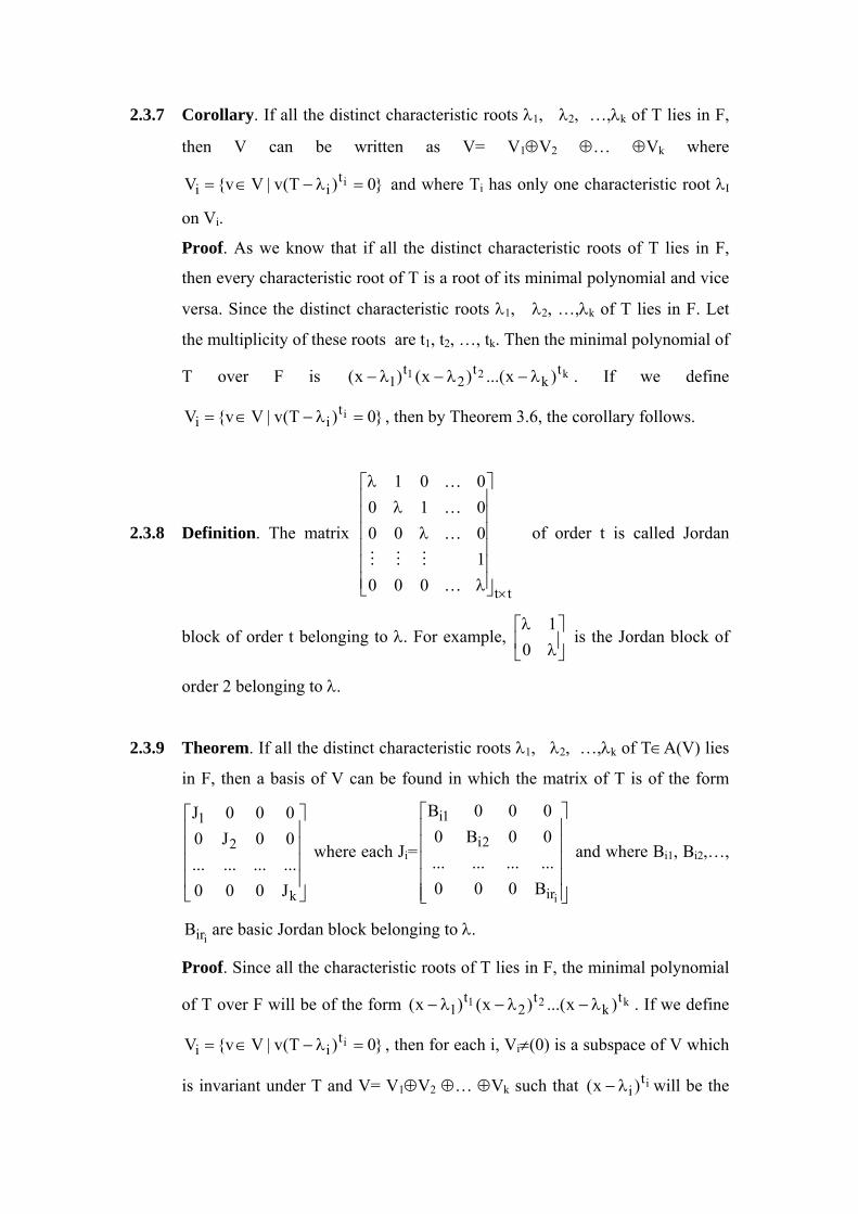
2.3.7 Corollary. If all the distinct characteristic roots λ1, λ2, …,λk of T lies in F,

then V can be written as V= V1⊕V2 ⊕… ⊕Vk where

}0)T(v|Vv{V itii =λ−∈= and where Ti has only one characteristic root λI

on Vi.

Proof. As we know that if all the distinct characteristic roots of T lies in F,

then every characteristic root of T is a root of its minimal polynomial and vice

versa. Since the distinct characteristic roots λ1, λ2, …,λk of T lies in F. Let

the multiplicity of these roots are t1, t2, …, tk. Then the minimal polynomial of

T over F is k21 tk

t2

t1 )x...()x()x( λ−λ−λ− . If we define

}0)T(v|Vv{V itii =λ−∈= , then by Theorem 3.6, the corollary follows.

2.3.8 Definition. The matrix

tt0001000010001

×⎥⎥⎥⎥⎥⎥

⎦

⎤

⎢⎢⎢⎢⎢⎢

⎣

⎡

λ

λλ

λ

K

MMM

K

K

K

of order t is called Jordan

block of order t belonging to λ. For example, ⎥⎦

⎤⎢⎣

⎡λ

λ0

1 is the Jordan block of

order 2 belonging to λ.

2.3.9 Theorem. If all the distinct characteristic roots λ1, λ2, …,λk of T∈A(V) lies

in F, then a basis of V can be found in which the matrix of T is of the form

⎥⎥⎥⎥

⎦

⎤

⎢⎢⎢⎢

⎣

⎡

k

2

1

J000............00J0000J

where each Ji=

⎥⎥⎥⎥⎥

⎦

⎤

⎢⎢⎢⎢⎢

⎣

⎡

iir

2i

1i

B000............00B0000B

and where Bi1, Bi2,…,

iirB are basic Jordan block belonging to λ.

Proof. Since all the characteristic roots of T lies in F, the minimal polynomial

of T over F will be of the form k21 tk

t2

t1 )x...()x()x( λ−λ−λ− . If we define

}0)T(v|Vv{V itii =λ−∈= , then for each i, Vi≠(0) is a subspace of V which

is invariant under T and V= V1⊕V2 ⊕… ⊕Vk such that iti )x( λ− will be the

minimal polynomial of Ti. As we know that if V is direct sum of its subspaces

invariant under T, then we can find a basis of V in which the matrix of T is of

the form

⎥⎥⎥⎥

⎦

⎤

⎢⎢⎢⎢

⎣

⎡

k

2

1

J000............00J0000J

, where each Ji is the ni×ni matrix of Ti (the

transformation induced by T on Vi) under the basis of Vi. Since the minimal

polynomial of Ti on Vi is iti )x( λ− , therefore, )IT( iλ− is nilpotent

transformation on Vi with index of nilpotence ti. But then we can obtain a

basis Xi of Vi in which the matrix of )IT( iλ− is of the form.

iii nnir

2i

1i

M000............00M0000M

×⎥⎥⎥⎥⎥

⎦

⎤

⎢⎢⎢⎢⎢

⎣

⎡

where i1≥ i2 ≥ … ≥ iri; i1+ i2+ …

+ iri= ni=dim Vi. Since Ti=λiI+ Ti-λiI, therefore, the matrix of Ti in the basis Xi

of Vi is Ji= matrix of λiI under the basis Xi + matrix of Ti -λiI under the basis

Xi. Hence Ji=

ii nn000............000000

×⎥⎥⎥⎥

⎦

⎤

⎢⎢⎢⎢

⎣

⎡

λ

λλ

+

iii nnir

2i

1i

M000............00M0000M

×⎥⎥⎥⎥⎥

⎦

⎤

⎢⎢⎢⎢⎢

⎣

⎡

=

⎥⎥⎥⎥⎥

⎦

⎤

⎢⎢⎢⎢⎢

⎣

⎡

iir

2i

1i

B000............00B0000B

, Bij are basic Jordan blocks. It proves the result.

2.4 CANONICAL FORM(RATIONAL FORM)

2.4.1 Definition. An abelian group M is called module over a ring R or R-module if

rm ∈ M for all r∈R and m∈M and

(i) (r + s)m=rm + rs

(ii) r(m1 + m2) = rm1 + rm2

(iii) (rs)m = r(sm) for all r, s ∈R and m, m1, m2∈M.

2.4.2 Definition. Let V be a vector space over the field F and T∈A(V). For f(x) ∈

F[x], define, f(x)v=vf(T) , f(x) ∈ F[x] and v∈V. Under this multiplication V

becomes an F[x]-module.

2.4.3 Definition. An R-module M is called cyclic module if M ={rm0 | r∈R and

some m0∈M.

2.4.4 Result. If M is finitely generated module over a principal ideal domain R.

Then M can be written as direct sum of finite number of cyclic R-modules. i.e.

there exist x1 , x2, …, xn in M such that

M=Rx1 ⊕Rx2 ⊕… ⊕Rxn.

2.4.5 Definition. Let f(x)= a0 + a1x + …+am-1 xm-1 + xm be a polynomial over the

field F. Then the companion matrix of f(x) is

mm1m10 a...aa1.........0000010

×−⎥⎥⎥⎥

⎦

⎤

⎢⎢⎢⎢

⎣

⎡

−−−

O.

It is a square matrix [bij] of order m such that bi, i+1=1 for 1 ≤ i ≤ m-1, bm, j= aj-1

for 1 ≤ j ≤ m and for the rest of entries bij=0. The above matrix is called

companion matrix of f(x). It is denoted by C(f(x)). For example companion

matrix of 1+2x -5x2 +4x3 + x4 is

444521100001000010

×⎥⎥⎥⎥

⎦

⎤

⎢⎢⎢⎢

⎣

⎡

−−−

2.4.6 Note. Every F[x]-module M becomes a vector space over F.Under the

multiplication f(x)v = vf(T), T∈ A(V) and v ∈ V, V becomes a vector space

over F.

2.4.7 Theorem. Let V be a vector space over F and T∈A(V). If f(x) = a0 + a1x +

…+am-1 xm-1 + xm is minimal polynomial of T over F and V is cyclic F[x]-

module, then there exist a basis of V under which the matrix of T is

companion matrix of f(x).

Proof. Clearly V becomes F[x]-module under the multiplication defined by

f(x)v= vf(T) for all v∈V , T∈A(V). As V is cyclic F[x]-module, therefore,

there exist v0∈V such that V = F[x]v0 ={ f(x)v0 | f(x)∈F[x]}= { v0f(T) |

f(x)∈ F[x]}. Now we will show that if v0s(T)=0, then s(T) is zero

transformation on V. Since v = f(x)v0 , then vs(T) = (f(x)v0)s(T)= (v0 f(T))s(T)

= (v0 s(T))f(T)= 0f(T)=0. i.e. every element of v is taken to 0 by s(T). Hence

s(T) is zero transformation on V. In other words T also satisfies s(T). But then

f(x) divides s(x). Hence we have shown that for a polynomial s(x)∈F[x], if

v0s(T) =0, then f(x) | s(x).

Now consider the set A={v0, v0T,…, v0Tm-1 } of elements of V.

We will show that it is required basis of V. Take r0v0 + r1 (v0T) +…+ rm-1

( v0Tm-1) =0, ri∈F. Further suppose that at least one of ri is non zero. Then r0v0

+ r1 (v0T) + … + rm-1 ( v0Tm-1) = 0 ⇒ v0 (r0+ r1 T + … + rm-1 Tm-1) =0.

Then by above discussion f(x)| (r0+ r1 T + … + rm-1 Tm-1), a contradiction.

Hence if r0v0 + r1 (v0T) +…+ rm-1 ( v0Tm-1) =0 then each ri =0. ie the set

A is linearly independent over F.

Take v∈V. Then v = t(x)v0 for some t(x)∈F[x]. As we can

write t(x)= f(x)q(x) + r(x), r(x) = r0+ r1x + … + rm-1xm-1 , therefore, t(T)=

f(T)q(T) + r(T) where r(T)= r0+ r1 T + … + rm-1 Tm-1. Hence v = t(x)v0 =

v0t(T) = v0(f(T)q(T) +r(T)) = v0f(T)q(T) + v0r(T) = v0r(T) = v0 (r0+ r1 T + …

+ rm-1 Tm-1)= r0v0 + r1 (v0T) + … + rm-1 ( v0Tm-1). Hence every element

of V is linear combination of element of the set A over F. Therefore, A is a

basis of V over F.

Let v1 =v0, v2 =v0T, v3 =v0T2, …, vm-1 =v0Tm-2 , vm =v0Tm-1.

Then

v1T= v2 = 0.v1 + 1.v2 + 0.v3 + …+0. vm-1 +0vm,

v2T= v3 = 0.v1 + 0.v2 + 1.v3 + …+0. vm-1 +0vm,

… … … …,

vm-1T= vm = 0.v1 + 0.v2 + 0.v3 + …+0. vm-1 +1vm.

Since f(T)=0 ⇒ v0 f(T) = 0 ⇒ v0(a0 + a1T + …+am-1Tm-1 + Tm) = 0

⇒a0 v0+ a1 v0T + …+am-1 v0Tm-1 + v0Tm=0

⇒ v0Tm= -a0 v0 - a1 v0T - …- am-1 v0Tm-1 .

As vmT= v0Tm-1T=v0Tm = -a0 v0 - a1 v0T - …- am-1 v0Tm-1

= -a0 v1 - a1 v2 - …- am-1 vm.

Hence the matrix under the basis v1 =v0, v2 =v0T, v3 =v0T2, …, vm-1 =v0Tm-2 ,

vm =v0Tm-1 is

mm1m10 aaa10000000010

×−⎥⎥⎥⎥

⎦

⎤

⎢⎢⎢⎢

⎣

⎡

−−− L

O= C(f(x)). It proves the result.

2.4.8 Theorem. Let V be a finite dimensional vector space over F and T∈A(V).

Suppose q(x)t is the minimal polynomial for T over F, where q(x) is

irreducible monic polynomial over F . Then there exist a basis of V such that

the matrix of T under this basis is of the form

⎥⎥⎥⎥⎥

⎦

⎤

⎢⎢⎢⎢⎢

⎣

⎡

))x(q(C0000

0))x(q(C000))x(q(C

k

2

1

t

t

t

L

ML

L

L

where t=t1≥ t2 ≥…≥tk.

Proof. Since we know that if M is a finitely generated module over a principal

ideal domain R, then M can be written as direct sum of finite number of cyclic

R-submodules. We know that V is a vector space over F[x] with the scalar

multiplication defined by f(x)v=vf(T). As V is a finite dimensional vector

space over F, therefore, it is finitely dimensional vector space over F[x] also.

Thus, it is finitely generated module over F[x] (because each vector space is a

module also). But then we can obtain cyclic submodules of V say F[x]v1,

F[x]v2, …, F[x]vk such that V = F[x]v1 ⊕ F[x]v2 ⊕ … ⊕F[x]vk, vi∈V.

Since (F(x)vi ) T =(vi F[T]) T = =vi (F[T] T) = =(vi g(T))=

g(x)vi ∈ F[x]vi . Hence each F[x]vi is invariant under T. But then we can find

a basis of V in which the matrix of T is

⎥⎥⎥⎥

⎦

⎤

⎢⎢⎢⎢

⎣

⎡

k

2

1

A0000

0A000A

L

ML

L

L

where Ai is the

matrix of T under the basis of Vi. Now we claim that ))x(q(CA iti = . Let

pi(x) be the minimal polynomial of Ti (i.e of T on Vi). Since wi q(T)t = 0 for

all wi∈ F[x]vi, therefore, pi(x) divides q(x)t. Thus iti )x(qp = . 1≤ ti ≤ t. Re

indexing Vi, we can find t1 ≥ t2 ≥ … ≥ tk. Since V = F[x]v1 ⊕ F[x]v2 ⊕ …

⊕F[x]vk, therefore, the minimal polynomial of T on V is

lcm( k21 ttt )x(q...,,)x(q,)x(q )= 1t)x(q . Then t)x(q = 1t)x(q . Hence t=t1. By

Theorem 2.4.7, the matrix of T on Vi is companion matrix of monic minimal

polynomial of T on Vi. Hence Ai = ))x(q(C it . It proves the result.

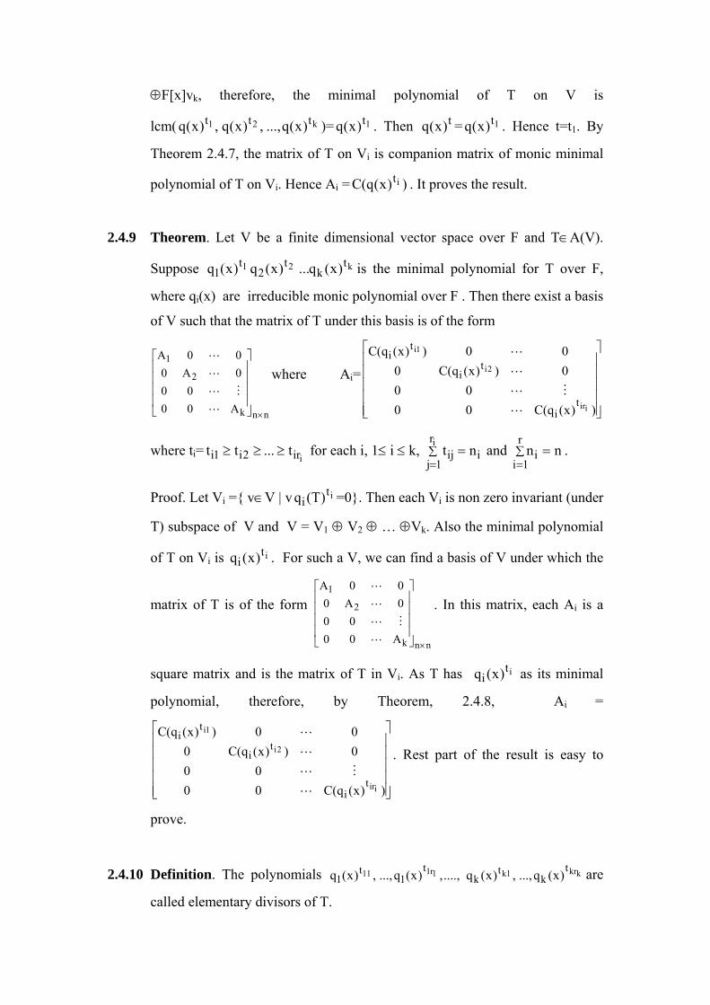
2.4.9 Theorem. Let V be a finite dimensional vector space over F and T∈A(V).

Suppose k21 tk

t2

t1 )x(q...)x(q)x(q is the minimal polynomial for T over F,

where qi(x) are irreducible monic polynomial over F . Then there exist a basis

of V such that the matrix of T under this basis is of the form

nnk

2

1

A0000

0A000A

×⎥⎥⎥⎥

⎦

⎤

⎢⎢⎢⎢

⎣

⎡

L

ML

L

L

where Ai=

⎥⎥⎥⎥⎥

⎦

⎤

⎢⎢⎢⎢⎢

⎣

⎡

))x(q(C0000

0))x(q(C000))x(q(C

iir

2i

1i

ti

ti

ti

L

ML

L

L

where ti= iir2i1i t...tt ≥≥≥ for each i, 1≤ i ≤ k, ir

1jij nt

i=∑

= and nn

r

1ii =∑

=.

Proof. Let Vi ={ v∈V | v iti )T(q =0}. Then each Vi is non zero invariant (under

T) subspace of V and V = V1 ⊕ V2 ⊕ … ⊕Vk. Also the minimal polynomial

of T on Vi is iti )x(q . For such a V, we can find a basis of V under which the

matrix of T is of the form

nnk

2

1

A0000

0A000A

×⎥⎥⎥⎥

⎦

⎤

⎢⎢⎢⎢

⎣

⎡

L

ML

L

L

. In this matrix, each Ai is a

square matrix and is the matrix of T in Vi. As T has iti )x(q as its minimal

polynomial, therefore, by Theorem, 2.4.8, Ai =

⎥⎥⎥⎥⎥

⎦

⎤

⎢⎢⎢⎢⎢

⎣

⎡

))x(q(C0000

0))x(q(C000))x(q(C

iir

2i

1i

ti

ti

ti

L

ML

L

L

. Rest part of the result is easy to

prove.

2.4.10 Definition. The polynomials kkr1k1r111 tk

tk

t1

t1 )x(q...,,)x(q....,,)x(q...,,)x(q are

called elementary divisors of T.

2.4.11 Theorem. Prove that elementary divisors of T are unique.

Proof. Let klkll xqxqxqxq )(...)()()( 21 21= be the minimal polynomial of T

where each qi(x) is irreducible and li ≥ 1. Let Vi= { v∈V| ili Tvq )( =0}. Then

Vi is a non zero invariant subspace of V, V=V1 ⊕V2⊕…⊕Vk and the minimal

polynomial of T on Vi i.e. of Ti , is ili )x(q . More over we can find a basis of

V such that the matrix of T is ⎥⎦

⎤⎢⎣

⎡

k

1R

R, where Ri is the matrix of T on Vi.

Since V becomes an F[x] module under the operation f(x)v=vf(T),

therefore, each Vi is also an F[x]-module. Hence there exist v1, v2, …, irv ∈ Vi

such that Vi= F[x]v1 +… +F[x]irv = Vi1 + Vi2 + … +

iirV where each Vij is a

subspace of Vi and hence of V . More over Vij is cyclic F[x] module also. Let

ijlxq )( be the minimal polynomials of T on Vij. Then ijlxq )( becomes

elementary divisors of T, 1 ≤ i ≤ k and 1≤ j ≤ ri. Thus to prove that elementary

divisors of T are unique, it is sufficient to prove that for all i, 1≤ i ≤ k, the

polynomials 1)( ili xq , 2)( ili xq ,…, iirli xq )( are unique. Equivalently, we have

to prove the result for T∈A(V), with q(x)l , q(x) is irreducible as the minimal

polynomial have unique elementary divisor.

Suppose V = V1 ⊕V2⊕…⊕Vr and V = W1 ⊕ W2⊕…⊕Ws where each

Vi and Wi is a cyclic F[x]-module. The minimal polynomial of T on Vi is

have unique elementary divisors ilxq )( where l=l1≥ l2 ≥ … ≥ lr and l=l*1≥ l*2

≥ … ≥ l*s . Also ∑=

r

iidl

1= n = dim V and ∑

=

s

idl

i1

* = dim V, d is the degree of

q(x). We will sow that li = l*i and r=s. Suppose t is first integer such that

l1=l*1, l2 =l*2 , …, lt-1= l*t-1 and lt ≠ l*t. Since each Vi and Wi are invariant

under T, therefore, ttt lr

ll TqVTqVTVq **1

* )(...)()( ⊕⊕= . But then the

dimension tlTVq *)( = tlj

r

jTqV *

1)(dim∑

=≥ tl

ji

jTqV *

1)(dim∑

=. Since lt ≠ l*t,

without loss of generality, suppose that lt > l*t. As tlj TqV *)( = d(lj -l*t),

therefore, dim tlTVq *)( ≥ ∑−

=−

1

1)*(

i

jtj lld . Similarly dimension of

ilTVq *)( = ∑−

=−

1

1)**(

i

jtj lld < ∑

=−

i

jtj lld

1)*( ≤ ilTVq *)( , a contradiction. Thus

lt ≤ l*t. Similarly, we can show that lt ≥ l*t. Hence lt = l*t . It holds for all t.

But then r = s.

2.5 KEY WORDS

Nilpotent Transformations, similar transformations, characteristic roots,

canonical forms.

2.6 SUMMARY

For T ∈A(V), V is finite dimensional vector space over F, we study nilpotent

transformation, Jordan forms and rational canonical forms.

2.7 SELF ASSESMENT QUESTIONS

(1) Show that all the characteristic root of a nilpotent transformations are zero

(2) If S and T are nilpotent transformations, then show that S+T and ST are

also nilpotent.

(3) Show that S and T are similar if and only they have same elementary

divisors.

2.8 SUGGESTED READINGS:

(1) Modern Algebra; SURJEET SINGH and QAZI ZAMEERUDDIN, Vikas

Publications.

(2) Basic Abstract Algebra; P.B. BHATTARAYA, S.K.JAIN, S.R.

NAGPAUL, Cambridge University Press, Second Edition.

MAL-521: M. Sc. Mathematics (Advance Abstract Algebra)

Lesson No. 3 Written by Dr. Pankaj Kumar

Lesson: Modules I Vetted by Dr. Nawneet Hooda

STRUCTURE

3.0 OBJECTIVE

3.1 INTRODUCTION

3.2 MODULES (CYCLIC MODULES)

3.3 SIMPLE MODULES

3.4 SIMI-SIMPLE MODULES

3.5 FREE MODULES

3.6 NOETHERIAN AND ARTINIAN MODULES

3.7 NOETHERIAN AND ARTINIAN RINGS

3.8 KEY WORDS

3.9 SUMMARY

3.10 SELF ASSESMENT QUESTIONS

3.11 SUGGESTED READINGS

3.0 OBJECTIVE

Objective of this chapter is to study another algebraic system

(modules over an arbitrary ring R) which is generalization of vector spaces

over field F.

3.1 INTRODUCTION

A vector space is an algebraic system with two binary operations over

a field F which satisfies certain conditions. If we take an arbitrary ring, then

vector space V becomes an R-module or a module over ring R.

In first section of this chapter we study definitions and examples of

modules. In section 3.3, we study about simple modules (i.e. modules having

no proper submodule). In next section, semi-simple modules are studied. Free

modules are studied in section 3.5. We also study ascending and descending

chain conditions for submodules of given module. There are certain modules

which satisfies ascending chain conditions (called as noetherian module) and

descending chain conditions (called as artinian modules). Such type of

modules are studied in section 3,6. At last we study noetherian and artinian

rings.

3.2 MODULES(CYCLIC MODULES)

3.2.1 Definition. Let R be a ring. An additive abelian group M together with a

scalar multiplication μ: R×M→M, is called a left R module if for all r, s∈R

and x, y ∈M

(i) μ(r, (x + y)) = μ(r, x) + μ(r, y)

(ii) μ((r + s), x) = μ(r, x) +μ(s, x)

(iii) μ(r, sx))= μ (rs, x)

If we denote μ(r, x) =rx, then above conditions are equivalent to

(i) r(x + y)) = rx + ry

(ii) (r + s) x = r x +s x

(iii) r (sx) = (rs) x.

If R has an identity element 1 and

(iv) 1x=x for all x ∈M. Then M is called Unitary (left) R-module

Note. If R is a division ring, then a unital (left) R-module is called as left

vector space over R.

Example (i) Let Z be the ring of integer and G be any abelian group with nx

defined by

nx = x + x +...+ x(n times) for positive n and

nx=-x-x-...-x(n times) for negative n and zero other wise.

Then G is an Z-module.

(ii) Every extension K of a field F is also an F-module.

(iii) R[x], the ring of polynomials over the ring R, is an R-module

3.2.2 Definition. Submodule. Let M be an R-module. Then a subset N of M is

called R-submodule of M if N itself becomes a module under the same scalar

multiplication defined on R and M. Equivalently, we say that if

(i) x-y∈N

(ii) rx∈N for all x, y∈N and r∈R.

Example (i) {0} and M are sub modules of R-module M. These are called

trivial submodules.

(ii) Since 2Z (set of all even integers) is an Z-module. Then 4Z, 8Z are its Z

submodules.

(iii) Each left ideal of a ring R is an R-submodule of left R-module and vice

versa.

3.2.3 Theorem. If M is an left R-module and x∈M, then the set Rx={rx| x∈R} is an

R-submodule of M.

Proof. As Rx ={rx| x∈R}, therefore, for r1 and r2 belonging to R, r1x and r2x

belongs to Rx. Since r1-r2 ∈R, therefore, r1x -r2x= (r1 -r2)x∈Rx. More over for

r and s∈R, s(rx)=(sr)x∈Rx. Hence Rx is an R-submodule of M.

3.2.4 Theorem. If M is an R-module and K={rx + nx| r∈R, n∈Z} is an R-

submodule of M containing x . Further if M is unital R-module then K=Rx.

Proof. Since for r1, r2 ∈R and n1, n2 ∈Z we have r1-r2 ∈R and n1-n2 ∈Z,

therefore, r1x+n1x–(r2x+n2x) = r1x – r2x + n1x – n2x = (r1–r2)x+(n1– n2)x ∈K.

More over for s∈R, s(rx + nx) = s(rx + x +… + x) = s(rx) + sx +…+ sx = (sr)x

+ sx +…+ sx= ((sr) + s + … + s)x. Since ((sr) + s + … + s)∈R, therefore, ((sr)

+ s +…+ s)x + 0.x ∈K. Hence K is an R-submodule. As x = 0x + 1x∈K,

therefore, K is an R-submodule containing x. Let S be another R-submodule

containing x, then rx and nx ∈S. Hence K ⊆ S. Therefore, K is the smallest R-

submodule containing x.

If M is unital R-module, then 1∈R such that 1.m=m∀ m∈M. Hence for

x ∈M, x=1.x ∈ Rx. As by Theorem 3.2.3, Rx is an R-submodule. But K is the

smallest R-submodule of M containing x. Hence K⊆Rx. Now For rx∈Rx,

rx=rx + 0x∈K. Hence K=Rx. It proves the theorem.

3.2.5 Definition. Let S be a subset of an R-module M. The submodule generated by

S, denoted by <S> is the smallest submodule of M containing S.

3.2.6 Theorem. Let S be a subset of an R-module M. Then <S> ={0} if S=φ, and is

C(S)={ r1 x1+r2 x2 + …+ rn xn| ri ∈R} if S={x1, x2, …, xn}.

Proof. Since < S > is the smallest submodule containing S, therefore, for the

case when S=φ, < S >= {0}. Suppose that S={x1, x2,…, xn}. Let x and y∈C(S).

Then x= r1 x1+r2 x2 + …+ rn xn, y= t1 x1+t2 x2 + …+ tn xn, ri and ti ∈R and x-y

= (r1−t1)x1+(r2−t2)x2+…+(rn−tn)xn ∈C(S). Similarly rx∈C(S) for all r∈R and

x∈C(S). Therefore, C(S) is a submodule of M. Further if N is another

submodule containing S then x1, x2, …, xn ∈ N and hence r1 x1+r2 x2 + …+ rn

xn ∈N i.e. C(S) ⊆ N. It shows that C(S) =<S>is the smallest such submodule.

3.2.7 Definition. Cyclic module. An R-module M is called cyclic module if it is

generated by single element of M. The cyclic module generated by x is and is

{rx+nx| r∈ R , n∈Z}. Further if M is an unital R-module, then < x > ={rx |

r∈R}.

Example.(i) Every finite additive abelian group is cyclic Z-module.

(ii) Every field F as an F-module is cyclic module.

3.3 SIMPLE MODULES

3.3.1 Definition. A module M is said to be simple R-module if RM≠{0} and the

only submodules of it are {0} and M.

3.3.2 Theorem. Let M be an unital R-module. Then M is said to be simple if and

only if M =Rx for every non zero x∈M. In other words M is simple if and

only if it is generated by every non zero element x ∈ M.

Proof. First suppose that M is simple. Consider Rx={rx | r∈R}. By Theorem

3.2.3, it is an R-submodule of M. As M is unital R-module, therefore, there

exist 1∈R such that 1.m=m for all m∈M. Hence x(≠0)=1.x ∈Rx, therefore Rx

is non zero unital R-module. Since M is simple, therefore, M=Rx. It proves the

result.

Conversely, suppose that M=Rx for every non zero x in M. Let

A be any non zero submodule of M. Then A ⊆ M. Let y be a non zero element

in A. Then y∈M. Hence by our assumption, M=Ry. By Theorem 3.2.3, Ry is

the smallest submodule containing y, therefore, Ry⊆A. hence M⊆A. Now

A⊆M, M⊆A implies that M=A i.e. M has no non zero submodule. Hence M is

simple.

3.3.3 Corollary. If R is a unitary ring. Then R is a simple R-module if and only if R

is a division ring.

Proof. First suppose that R is simple R-module. We will show that R is a

division ring. Let x be a non zero element in R. As R is a unitary simple ring,

therefore, by Theroem 3.2.8, R=Rx. As 1∈R and R=Rx, therefore, 1∈Rx.

Hence there exist a non-zero y in R such that 1=yx. i.e. inverse of non zero

element exist in R. Hence R is a division ring.

Conversely suppose that R is a division ring. Since ideals of a

ring are R-submodules of that ring and vice versa, therefore ideals of R will be

submodules of M. But R has two ideal {0} and R itself. Hence R has only

trivial submodules. Therefore, R is simple R-module.

3.3.4 Definition. A f be a mapping from an R-module M to an R-module N is called

homomorphism if

(i) f(x + y)=f(x) + f(y) (ii) f(rx)=rf(x) for all x, y ∈M and r∈R.

It is easy to see that f(0)=0, f(−x)= −f(x) (iii) f(x−y)=f(x) −f(y).

3.3.5 Theorem (Fundamental Theorem on Homomorphism). If f is an

homomorphism from R-modules M into N, then )M(ffker

M≅ .

3.3.6 Problem. Let R be a ring with unity and M be an R-module. Show that M is

cyclic if and only if M ≅IR , where I is left ideal of R.

Solution. First let M be cyclic i.e. M=Rx for some x∈M. Define a mapping

φ: R→M by φ(r) =rx, r∈R. Since φ(r1 + r2)= (r1 + r2)x=r1x + r2x =φ(r1) + φ(r2)

and φ(sr)= (sr)x = s(rx)=sφ(r) for all r1, r2, s and r belonging to R, therefore, φ

is an homomorphism from R to M. As M=Rx, therefore, for rx∈M, there exist

r ∈R such that φ(r) =rx i.e. the mapping is onto also. Hence by Fundamental

theorem on homorphism, MKer

R≅

φ. But Ker φ is an left ideal of R,

therefore, taking Ker φ=I we get M ≅IR .

Conversely suppose that M ≅IR . Let f :

IR→M be an isomorphism

such that f(1+I)=x. Then for r∈R, f(r+I) = f(r(1+I))=r f(1+I)=rx. i.e. we have

shown that img f = {rx| r∈R}=Rx. Since image of f is M, therefore, Rx =M

for some x∈M. Thus M is cyclic. It proves the result.

3.3.7 Theorem. Let N be a submodule of M. Prove that the submodules of the

quotient module NM are of the form

NU , where U is submodule of M

containing N.

Proof. Define a mapping f: M→NM by f(m)=m+N ∀ m∈M. Let X be an

submodule of NM . Define U={x∈M| f(x)∈X}= { x∈M | m + N ∈X }. Let x,

y∈U. Then f(x), f(y) ∈X . But then f(x−y) = f(x)−f(y) ∈X and for r∈R,

f(rx)=rf(x) ∈X . Hence by definition of U, x−y and rx∈U. i.e. U is an R-

submodule. Also N ⊆ U, because for all x∈N, f(x) = x + N = N = identity of

X, therefore, f(x)∈M. Because f is an onto mapping, therefore, for x∈X, there

always exists y ∈M, such that f(y)=x. By definition of U, y∈U. Hence X ⊆

f(U). Clearly f(U) ⊆ X. Thus X=f(U). But f(U) = NU . Hence X =

NU . It proves

the result.

3.3.8 Theorem. Let M be an unital R-module. Then the following are equivalent

(i) M is simple R-module

(ii) Every non zero element of M generates M

(iii) M ≅IR , where I is maximal left ideal of R.

Proof. (i)⇒(ii) follows from Theroem 3.2.8.

(ii) ⇒(iii). As every non zero element of M generates M, therefore, M is cyclic

and by Problem 3.2.12, M ≅IR . Now we have to show that I is maximal.

Since M is simple, therefore, IR is also simple. But then I is maximal ideal of

R. It proves (iii)

(iii) ⇒(i). By (iii) M ≅IR , I is maximal left ideal of R. Since I is maximal

ideal of R, therefore, I ≠ R. Further 1+I ∈IR and R(

IR )≠{I} implies that RM

≠{0}. Let N be a submodule of M and f is an isomorphism from M to IR .

Since f(N) is a submodule of IR , therefore, by Theorem 3.3.7, f(N) =

IJ . But I

is maximal ideal of R, therefore, J=I or J=R. If J=I, then f(N) = {I} implies

that N={0}. If J=R, then f(N)= IR implies that N=M. Hence M has no non-

trivial submodule i.e. M is simple.

3.3.9 Theorem. (Schur’s lemma). For a simple R-module M, HomR(M, M) is a

division ring.

Proof. Since the set of all homomorphism from M to M form the ring under

the operation defines by (f +g) (x)=f(x) + g(x) and (f.g)(x)=f(g(x)) for all f and

g belonging to the set of all homomorphism and for all x belonging to M. In

order to show that HomR(M, M) is a division ring we have to show that every

non zero homomorphism f has an inverse in HomR(M, M). i.e. we have to

show that f is one-one and onto. As f : M→M. consider Ker f and img f. Both

are submodules of M. But M is simple, therefore, ker f={0} or M. If ker f =M,

then f becomes a zero homomorphism. But f is non zero homomorphism.

Hence ker f ={0}. i.e. f is one-one.

Similarly img f={0} or M. If img f={0}, then f becomes an zero

mapping which is not true. Hence img f =M i.e. mapping is onto also. Hence f

is invertible. Therefore, we have shown that every non zero element of

HomR(M, M) is invertible. It mean HomR(M, M) is division ring.

3.4 SEMI-SIMPLE MODULES

3.4.1 Definition. Let M be an R-module and (Ni), 1≤ i≤ t be a family of submodules

of M. The submodule generated by Ut

1iiN

= is the smallest submodule

containing all the submodules Ni. It is also called the sum of submodules Ni

and is denoted by ∑=

t

1iiN .

3.4.2 Theorem. Let M be an R-module and (Ni), 1≤ i≤ t be a family of submodules

of M. Show that ∑=

t

1iiN ={x1+ x2 + … +xt | xi∈Ni}.

Proof. Let S={x1+ x2 + … +xt | xi∈Ni}. Further let x and y∈S. Then x= x1+ x2

+ …+ xn, y= y1 +y2 + …+ yn , xi and yi ∈S. Then x−y =( x1 + x2 + …+ xn) −

(y1 + y2 + …+ yn )= (x1−y1) + (x2−y2) +…+(xn−yn) ∈S . Similarly rx∈S for all

r∈R and x∈S. Therefore, S is an submodule of M.

Further if N is another left submodule containing S then x1,

x2, …, xn ∈ N and hence x1+ x2 + …+ xn ∈N i.e. S ⊆ N. It shows that S is the

smallest module containing each Ni. Therefore, by Definition 3.4.1, ∑=

t

1iiN =

S={x1+ x2 + … +xt | xi∈Ni}.

3.4.3 Note. If U iN is a family of submodules of M, then }Nx|x{Nfinite

iiii

i ∑∑Λ∈

∈= .

3.4.4 Definition. Let Λ∈ii )N( be a family of submodule M. The sum ∑Λ∈i

iN is called

direct sum if each element x of ∑Λ∈i

iN can be uniquely written as x =∑ ix ,

where xi ∈Ni and xi =0 for almost all i in index set Λ. In other words, there are

finite number of xi that are non zero in ∑ ix . It is denoted by ∑Λ∈

⊕i

iN . Each

Ni in ∑Λ∈

⊕i

iN is called a direct summand of the direct sum ∑Λ∈

⊕i

iN .

3.4.5 Theroem. Let Λ∈ii )N( be a family of submodule M. Then the following are

equivalent.

(i) ∑Λ∈i

iN is direct

(ii) }0{NN

ijj

ji =∩ ∑

≠Λ∈

for all i

(iii) 0=∑ ix ∈ ∑Λ∈i

iN ⇒ xi = 0 for all i.

Proof. These results are easy to prove.

3.4.6 Definition. (Semi-simple module). An R-module M is called semi-simple or

completely reducible if M = ∑Λ∈i

iN , where Ni’s are simple R-submodules of M.

Example. R3 is a semi-simple R-module.

3.4.7 Theorem. Let M = ∑Λ∈α

αM be a sum of simple R-submodules Mα and K be a

submodule of M. Then there exist a subset Λ* ⊆ Λ such that ∑Λ∈α

α*

M is a

direct sum and M= )M(K*

∑Λ∈α

α⊕⊕ .

Proof. Let S={Λ** ⊆ Λ | ∑Λ∈α

α**

M is a direct sum and K ∩ ∑Λ∈α

α**

M ={0}}.

Since φ ⊆ Λ and ∑φ∈α

αM ={0}, therefore, K ∩ ∑φ∈α

αM =K∩{0}={0}. Hence

φ∈S. Therefore, S is non empty. Further S is partial order set under the

relation that for A, B ∈S, A is in relation with B iff either A ⊆ B or B ⊆ A.

More over every chain (Ai) in S has an upper bound ∪Ai in S. Thus by Zorn’s

lemma S has maximal element say Λ*. Let N= )M(K*

∑Λ∈α

α⊕⊕ . We will

show that N=M. Let ω ∈Λ. Since Mω is simple, therefore, either N∩Mω ={0}

or Mω. If N∩Mω = {0}, then }0{)M(M*

=⊕∩ ∑Λ∈α

αω . But then

∑ω∪Λ∈α

α}{*M is a direct sum having non empty intersection with K. But this

contradicts the maximality of Λ*. Thus N ∩ Mω = Mω i.e. Mω ⊆ N, proving

that N=M.

3.4.8 Note. If we take K={0} module in Theorem 3.4.7, then we get the result that

“ If M = ∑Λ∈α

αM is the sum of simple R-submodules Mα , then there exist a

subset Λ* ⊆ Λ such that ∑Λ∈α

α*

M is a direct sum and M= ∑Λ∈α

α⊕*

M ”.

3.4.9 Theorem. Let M be an R-module. Then the following conditions are

equivalents

(i) M is semi-simple

(ii) M is direct sum of simple modules

(iii) Every submodule of M is direct summand of M.

Proof. (i)⇒(ii). Since M is semi-simple, then by definition, M = ∑Λ∈α

αM ,

where Ni’s are simple submodules. Also by Theorem 3.4.7, if M = ∑Λ∈α

αM is a

sum of simple R-submodules Mα’s and K be a submodule of M, then there

exist a subset Λ* ⊆ Λ such that ∑Λ∈α

α*

M is a direct sum and

M= )M(K*

∑Λ∈α

α⊕⊕ . By Note 3.4.8, if we take K={0}, then M = ∑Λ∈α

α⊕*

M

i.e. M is direct sum of simple submodules.

(ii) ⇒(iii). Let M = ∑Λ∈α

α⊕ M , where each Mα is simple. Then M is sum of

simple R-submodules. But then by Theorem 3.4.7, for given submodule K of

M we can find a subfamily Λ* of given family Λ of submodules such that

M= )M(K*

∑Λ∈α

α⊕⊕ . Take ∑Λ∈α

α⊕*

M =M*. Then M= *MK⊕ .Therefore, K

is direct summand of M.

(iii) ⇒(i). First we will show that M has simple submodule. Let N=Rx be a

submodule of M. Since N is finitely generated module, therefore, N has a

maximal element N* (say) (because every finitely generated module has a

maximal element). Consider the quotient module *N

N . Since N* is simple,

therefore, *N

N is simple. Being a submodule of N, N* is submodule of M

also. Hence N* is a direct summand of M. Therefore, there exist submodule

M1 of M such that M=N*⊕M1. But then N ⊆ N*⊕M1. If y∈N, then y = x + z

where x∈N* and z∈M1. Since z = y-x ∈N (because y ∈N and x∈N*⊆N),

therefore, y-x ∈N∩M1. Equivalently, y∈N* + N∩M1. Hence N⊆N* + N∩M1.

Since N* and N∩M1 both are subset of N, therefore, N* + N∩M1 ⊆ N. By

above discussion we conclude that N* +N∩M1 = N. Since M =N*⊕M1,

(N*∩ M1) = {0}, therefore, N*∩(N∩M1) = (N*∩ M1)∩N ={0}. Hence N=

N* ⊕ (N∩M1).

Now 11

1

11 MN}0{MN

)MN(*NMN

*NMN*N

*NN

∩≈∩

=∩∩

∩≅

∩+= .

Since *N

N is simple submodule, therefore, (N∩M1) is also simple submodule

of N and hence of M also. By above discussion we conclude that M always

has a simple submodule. Take ƒ={Mω}ω∈Λ as the family of all simple

submodules of M. Then by above discussion ƒ ≠ φ. Let X= ∑Λ∈ω

ωM . Then X is

a submodule of M. By (iii), X is direct summand of M, therefore, there exist

M* such that M=X⊕M*. We will show that M*={0}. If M* is non zero, then

M* has simple submodule say Y. Then Y∈ƒ. Hence Y⊆X. But then

Y=X∩M*, a contradiction to the result M=X⊕M*. Hence M*={0} and M=

X= ∑Λ∈ω

ωM i.e. M is semi-simple and (i) follows.

3.4.10 Theorem. Prove that submodule and factor modules of a semi-simple module

are again a semi-simple.

Proof. Let M be semi-simple R-module and N be a submodule of M. As M is

semi-simple, therefore, every submodule of M is direct summand of M. Hence

for given submodule X, there exist M* such that M =X⊕M*. But then

N=M∩N= X⊕M*∩N=(X∩N)⊕(M*∩N) . Hence X∩N is direct summand of

N. Therefore N is semi-simple.

Now we will show that NM is also semi-simple. Since M is semi-

simple and N is a submodule of M, therefore, N is direct summand of of M i.e.

M= N⊕M*. Since N∩M*={0}, therefore,

NM = *M

}0{*M

*MN*M

N*MN

==∩

≅⊕ . Being a submodule of semi-simple

module M, M* is semi-simple and hence NM is semi-simple. It proves the

result.

3.5 FREE MODULES

3.5.1 Definition. Let M be an R module. A subset S of M is said to be linearly

dependent over R if and only if there exist distinct elements x1, x2, …, xn in S

and elements r1, r2, …,rn in R, not all zero such that r1x1+r2x2+…+rnxn=0.

3.5.2 Definition. If the elements x1, x2, …, xn of M are not linearly dependent over

R, then we say that x1, x2, …, xn are linearly independent over R. A subset S=

{x1, x2, …, xt}of M is called linearly independent over ring R if elements x1,

x2, …, xt are linearly independent over R.

3.5.3 Definition. Let M be an R-module. A subset S of M is called basis of M over

R if

(i) S is linearly independent over R,

(ii) <S> = M. i.e. S generates M over R.

3.5.4 Definition. An R-module M is said to be free module if and only it has a basis

over R

Example(i) Every vector space V over a field F is a free F-module.

(ii) Every unitary R-module, R is a free R-module.

(iii) Every Infinite abelian group is a free Z-module.

Example of an R-module M which is not free module. Show that Q (the

field of rational numbers ) is not a free Z-module.(Here Z is the ring of

integers).

Solution. Take two non-zero rational numbers qp and

sr . Then there exist two

integers qr and -ps such that 0)srps(

qpqr =−+ . i.e. every subset S of Q

having two elements is Linearly dependent over Z. Hence every super set of S

i.e. every subset of Q having at least two elements is linearly dependent over

Z. Therefore, basis of Q over Z has at most one element. We will show the set

containing single element can not be a basis of Q over Z. Let qp be the basis

element. Then by definition of basis, Q={nqp , n∈Z}. But

q2p belongs to Q

such that q2p =

qp

21 ≠n

qp . Hence Q≠{n

qp , n∈Z}. In other word Q has no basis

over Z. Hence Q is not free module over Z.

3.5.5 Theorem. Prove that every free R-module M with basis {x1, x2, …, xt} is

isomorphic to R(t). (Here R(t) is the R-module of t-tuples over R).

Proof. Since {x1, x2, …, xt} is the basis of M over R, therefore, M={r1x1+ r2x2

+… + rtxt | r1, r2 ,…, rt∈R}. As R(t)={(r1, r2, …, rt)| r1, r2 ,…, rt∈R }. Define a

mapping f : M→R(t) by setting f(r1x1+ r2x2 +… + rtxt)=(r1, r2, …, rt). We will

show that f is an isomorphism.

Let x and y ∈M, then x= r1x1+ r2x2 +… + rtxt and y= s1x1+ s2x2 +… +

stxt where for each i, si and ri ∈R. Then

f(x+y)= f((r1+s1) x1+ (r2 + s2 )x2 +… + (rt + st )xt )

=((r1+s1), (r2+s2 ), … , (rt+st )) = (r1 , r2, … , rt ) + (s1, s2 , … , st )

= f(x)+f(y)

and f(rx)= f(r(r1x1+ r2x2 +… + rtxt)= f(rr1x1+r r2x2 +… + rrtxt)= (rr1, rr2, … rrt)

= r(r1, r2, … rt)= rf(x). Therefore, f is an R-homomorphism.

This mapping f is onto also as for (r1, r2, … rt)∈R(t) , there exist x = r1x1+ r2x2

+… + rtxt∈M such that f(x)= (r1, r2, … rt). Further f(x)=f(y)⇒ (r1, r2, … rt)

=(s1, s2 , … , st ) ⇒ ri =si for each i. Hence x=y i.e. the mapping f is one-one

also and hence the mapping f is an isomorphism from M to R(t).

3.6 NOETHERIAN AND ARTINIAN MODULES

3.6.1 Definition. Let M be a left R-module and {Mi}i≥1 be a family of submodules

of M . The family {Mi}i≥1 is called ascending chain if M1⊆ M2⊆… ⊆Mn⊆…

Similarly if M1⊇ M2⊇… ⊇Mn⊇…, then family {Mi}i≥1 is called descending

chain.

3.6.2 Definition. An R-module M is called Noetherian if for every ascending chain

of submodules of M, there exist an integer k such that Mk=Mk+t for all t ≥ 0. In

other words Mk=Mk+1= Mk+2 =… . Equivalently, an R-module M is called

Noetherian if every ascending chain becomes stationary or terminates after a

finite number of terms.

If the left R-module M is Noetherian, then M is called left Noetherian

and if right R-module M is Noetherian, then M is called right Noetherian.

Example. Show that Z as Z-module is Noetherian.

Solution. Since we know that Z is principal ideal ring and in a ring every ideal

is submodule of Z-module Z. Consider the submodule generated by <n>, n∈Z.

Further <n> ⊆ <m> iff m|n. As the number of divisors of n are finite,

therefore, the number of distinct member in the ascending chain of family of

submodules are finite. Hence Z is noetherian Z-module.

3.6.3 Theorem. Prove that for an left R-module M, following conditions are

equivalent:

(i) M is Noetherian (ii) Every non empty family of R -module has a

maximal element (iii) Every submodule of M is finitely generated.

Proof. (i) ⇒(ii). Let ƒ be a non empty family of submodules of M. If possible

ƒ does not have a maximal element, then for M1 ∈ ƒ, there exist M2 such that

M1 ⊆ M2. By our assumption, there exist M3, such that M1⊆M2⊆M3.

Continuing in this way we get an non terminating ascending chain M1

⊆M2⊆M3…. , of submodules of M, a contradiction to the fact that M is

Noetherian . Hence ƒ always have a maximal element.

(ii)⇒(iii). Consider a submodule N of M. Let xi∈N for i=1, 2, 3, … Consider

the family ƒ of submodules M1=<x1> , M2=<x1 , x2>, M3= < x1 , x2 , x3 >, … ,

of N or equivalently of M. By (ii), ƒ has maximal element Mk(say). Definitely

Mk is finitely generated. In order to show that N is finitely generated, it is

sufficient to show that Mk=N. Trivially Mk ⊆ N. Let xi∈N. Then xi∈Mi ⊆Mk

for all i. Hence N⊆Mk i.e. Mk=N. It proves (iii).

(ii)⇒(iii). Let ƒ be an ascending chain of submodules of M. and ascending

chain is M1⊆M2⊆M3… . Consider N = U1i

iM≥

. Then N is a submodule of M.

By (iii), N is finitely generated i.e. N=<x1, x2, …, xk>. Let Mt be the

submodule in the ascending chain M1⊆M2⊆M3… . such that each xi is

contained in Mt. Then N⊆Mr for all r ≥ t. But Mr ⊆N. Then N=Mr. Hence

Mt=Mt+1=Mt+2=… and hence M is Noetherian. It proves (i).

3.6.4 Definition. Let M be an left R-module and ζ ={Mλ}λ∈Λ be a non empty family

of submodules of M. M is called finitely co-generated if for every non empty

family ζ having {0} intersection has a finite subfamily with {0} intersection.

3.6.5 Definition. Left R-module M is called Left Artinian module if every

descending chain M1⊇M2⊇M3… of submodules of M becomes stationary after

a finite number of steps. i.e there exist k such that Mk=Mk+t for all t≥0.

3.6.6 Theorem. Prove that for an left R-module M, following conditions are

equivalent:

(i) M is Artinian (ii) Every non empty family of R-module has a minimal

element (iii) Every quotient module of M is finitely co-generated.

Proof. (i)⇒(ii). Let ƒ be a non empty family of submodules of M. If possible

ƒ does not have a minimal element, then for M1∈ ƒ, there exist M2 such that

M1⊇M2. By our assumption, there exist M3, such that M1⊇M2⊇M3 .

Continuing in this way we get an non terminating discending chain M1

⊇M2⊇M3…. , of submodules of M, a contradiction to the fact that M is

Artinian. Hence ƒ always have a minimal element.

(ii)⇒(iii). For a submodule N, consider the quotient module NM . Let

Λ∈λλ}

NM{ be a family of submodules of

NM such that I

Λ∈λ

λN

M ={N}. Since

N

M

NMN

I

I Λ∈λλ

Λ∈λ

λ == , therefore NM =Λ∈λ

λI . Let Λ∈λλ=ζ }M{ and for

every finite subset Λ* ⊆Λ let f ={A = I*MΛ∈λ

λ }. As Mλ ∈ f for all λ∈Λ,

therefore, ζ ⊆ f . i.e. f≠φ. By given condition f has a minimal element say A.

Then A= n21 M...MM λλλ ∩∩∩ . Let λ∈Λ. Then A ∩ Mλ ⊆A. But A is

minimal element of the collection f, therefore, A ∩ Mλ ≠(0). Hence A ∩ Mλ

=A ∀ λ∈Λ. But then A IΛ∈λ

λ⊆ M =N. Since N is contained in each Mλ ,

therefore, N ⊆ n21 M...MM λλλ ∩∩∩ =A. Hence N=A= In

1i iM

=λ . Now

NNN

N

M

NM

n

1in

1i

ii === =

λ

=

λI

I . Hence there exist a subfamily ni1}NM

{ i≤≤

λ of the

family Λ∈λλ}

NM{ such that N

NMn

1ii =

=

λI . It shows that every quotient module

is finitely co-generated. It proves (iii).

(iii)⇒(i). Let M1 ⊇ M2⊇…⊇Mn⊇Mn+1⊇…be a descending chain of

submodules of M. Let N= I1i

iM≥

. Then N is a submodule of M. Consider the

family {N

Mi }i≥1 of submodules of NM . Since N

NN

N

M

NM 1i

ii === ≥

Λ∈λ

I

I and

NM is finitely co-generated, therefore, there exist a subfamily ni1}N

M{ i

≤≤λ of

the family {N

Mi }i≥1 such that NN

Mn

1ii =

=

λI . Let k= max={λ1, λ2, …λn}. Then

N

MN

M

NM

N k

n

1in

1i

ii === =

λ

=

λI

I ⇒ Mk=N. Now N = I1i

iM≥

⊆ Mk+i ⊆ Mk ⊆ N ⇒

Mk+i ⊆ Mk for all i≥0. Hence M is Artinian.

3.6.7 Theorem. Let M be Noetherian left R-module. Show that every submodule

and factor module of M are also Noetherian.

Proof. Since M is Noetherian, therefore, it is finitely generated. Being a

submodule of finitely module, N is also finitely generated. Hence N is also

Noetherian.

Consider factor module NM . Let

NA be its submodule. Then A is

submodule of M is Noetherian, therefore, A is finitely generated. Suppose A is

generated by x1, x2, …, xn. Take arbitrary element x + N of NA . Then x∈A.

Therefore, x =r1x1 + r2x2 + …rnxn, ri ∈ R. But then x +N=(r1x1 + r2 x2+ …+

rnxn) + N = r1 (x1 +N) + r2 ( x2+N)+…+rn (xn+N) i.e. x +N is linear

combination of (x1 +N), ( x2+N), …, (xn+N) over R. Equivalently, we have

shown that NA is finitely generated. Hence

NA is Noetherian. It proves the

result.

3.6.8 Theorem. Let M be an left R-module. If N is a submodule of M such that N

and NM both are Noetherian, then M is also Noetherian.

Proof. Let A be a submodule of M. In order to show M is Noetherian we will

show that A is finitely generated. Since A+N is a submodule of M conting N,

therefore, N

NA + is submodule of NM . Being a submodule of Noetherian

module N

NA + is finitely generated. As NA

AN

NA∩

≅+ , therefore,

NAA∩

is also finitely generated. Let NA

A∩

=<y1 + (A∩N), y2 + (A∩N), …, yk +

(A∩N)>. Further A ∩N is a submodule of Noetherian module N, therefore, it

is also finitely generated. Let (A∩N)= <x1 , x2 , …, xt >. Let x∈A. Then

x+(A∩N)∈NA

A∩

. Hence x+(A∩N)= r1( y1 + (A∩N))+ r2( y2 + (A∩N))+ …

+ rk(yk + (A∩N)), ri∈R . Then x + (A∩N)= (r1y1 + r2y2 + … + rkyk +

(A∩N)) or x - (r1y1 + r2y2 + … + rkyk )∈ (A∩N). Since (A∩N)= <x1 , x2 ,

…, xt >, therefore, x - (r1y1 + r2y2 + … + rkyk )= s1x1 + s2x2 + … + stxt.

Equivalently x = (r1y1 + r2y2 + … + rkyk ) + s1x1 + s2x2 + … + stxt, si∈R.

Now we have shown that every element of A is linear combination of

elements of the set { r1, r2, … , rk , s1, s2, … , st} i.e. A is finitely

generated. It proves the result.

3.6.9 Theorem. Let M be an left R-module and N be a submodule of M. Then M is

artinian iff both N and NM are Artinian.

Proof. Suppose that M is Artinian. We will show that every submodule and

quotient modules of M are Artinian.

Let N be a submodule of N. Consider the deccending chain N1 ⊇ N2

⊇ … ⊇Nk ⊇ Nk+1 ⊇… of submodules of N. But then it becomes a descending

chain of submodules of M also. Since M is Artinian, therefore, there exist a

positive integer k such that Nk =Nk+i ∀ i ≥0. Hence N is Artinian.

Let NM be a factor module of M. Consider a descending chain

N

M1 ⊇N

M2 ⊇…⊇N

Mk ⊇N

M 1k+ ⊇…, Mi are submodules of M

containing N and are contained in Mi-1. Thus we have a descending chain

M1 ⊇ M2 ⊇ … ⊇Mk ⊇ Mk+1 ⊇… of submodules of M. Since M is

Artinian, therefore, there exist a positive integer K such that Mk =Mk+i ∀ i ≥0.

But then N

MN

M ikk += ∀ i ≥0. Hence NM is Artinain.

Conversely suppose that both N and NM are Artinian submodules of

M. We will show that M is Artinian. Let N1 ⊇ N2 ⊇ … ⊇Nk ⊇ Nk+1 ⊇… be

the deccending chain of submodules of M. Since Ni+N is a submodule of M

containing N, therefore, for each i, N

NNi + is a submodule of NM such that

NNN

NNN 1ii +⊇

+ + . Consider descending chain

...N

NNN

NN...N

NNN

NN 1kk21 ⊇+

⊇+

⊇⊇+

⊇+ + of submodules of

NM . As

NM is Artinian, therefore, there exist a positive integer k1 such that

NNN

NNN ikk 11

+=

+ + for all i ≥ 0. But then NNNN ikk 11+=+ + for all i ≥

0.

Since Ni ∩ N is a submodule of an Artinian module N and Ni ∩ N ⊇

Ni+1 ∩ N for all i, therefore, for descending chain

...NN...NNNN k21 ⊇∩⊇⊇∩⊇∩ N1 ∩ N of submodules of N, there

exist a positive integer k2 such that NNNN ikk 22∩=∩ + for all i ≥ 0. Let

k=max{k1, k2}. Then NNNN ikk +=+ + and NNNN ikk ∩=∩ + for all i

≥ 0. Now we will show that if NNNN ikk +=+ + and NNNN ikk ∩=∩ + ,

then ikk NN += for all i ≥ 0. Let x∈Nk , then x∈Nk +N= NN ik ++ . Thus x=

y+z where y∈Nk+i and z∈N . Equivalently, x-y=z∈N. Since y∈Nk+i,

therefore, y∈Nk also. But then x-y=z also belongs to Nk . Hence z∈Nk∩N=

Nk+i∩N and hence z=x-y ∈Nk+i. Now x-y∈Nk+i and y∈Nk+i implies that

x∈Nk+i. In other words we have shown that ikk NN +⊆ . But then

ikk NN += for all i ≥ 0. It proves the result.

3.6.10 Theorem. Prove that R-homomorphic image of Noetherian(Artinian) left R-

module is again Noetherian(Artinian).

Proof. Since homomorphic image of an Noetherian(Artinian) module M is

f(M) where f is an homomorphism from M to R-module N. Being a factor

module of M, fKer

M is Noetherian(Artinian). As f(M)≅ fKer

M , therefore,

f(M) is also Noetherian(Artinian).

3.7 NOETHERIAN AND ARTINIAN RINGS

3.7.1 Definition. A ring R is said to satisfy ascending (descending) chain condition

denoted by acc(dcc) for ideals if and only if given any sequence of ideals I1, I2,

I3… of R with I1⊆ I2 ⊆ … ⊆ In ⊆ …(I1 ⊇ I2 ⊇ … ⊇ In ⊇ …), there exist an

positive integer n such that In=Im for all m≥n.

Similarly a ring R is said to satisfy ascending (descending ) chain

condition for left (right) ideals if and only if given any sequence of left ideals

I1, I2, I3… of R with I1⊆ I2 ⊆ … ⊆ In ⊆ …(I1 ⊇ I2 ⊇ … ⊇ In ⊇ …), there exist

an positive integer n such that In=Im for all m ≥ n.

3.7.2 Definition. A ring R is said to be Notherian(Artinian) ring if and only if it

satisfies the ascending ()chain conditions for ideals of R. Similarly for non

commutative ring , a ring R is said to be left-Notherian(left-Notherian) ring if

and only if it satisfies the ascending chain conditions for left ideals (right

ideals) of R.

3.7.3 Definition. A ring R is said to satisfies the maximum condition if every non

empty set of ideals of R , partially ordered by inclusion, has a maximal

element.

3.7.4 Theorem. Let R be a ring then the following conditions are equivalent:

(i) R is Noetherian (ii) Maximal condition (for ideals) holds in R (iii) every

ideal of R is finitely generated.

Proof. (i) ⇒(ii). Let f be a family of non empty collection of ideals of R and

I1 ∈f. If I1 ∈ is not maximal element in f, then ther exist I2 ∈f such that I1⊆ I2.

Again if I2 is not maximal then there exist I3 ∈f such that I1⊆ I2 ⊆ I3. If f has

no maximal element, then continuing in this way we get an non terminating

ascending chain of ideal of R. But it is contradiction to (i) that R is noehterian.

Hence f has maximal element.

(ii) ⇒(iii). Let I be an ideal of R and f={A | A is an ideal of R, A is finitely

generated and A⊆I}. As {0}⊆I which is finitely generated ideal of R,

therefore, {0}∈f. By (ii), f has maximal element say M. We will show that

M=I. Suppose that M≠I, then there exist an element a∈I such that a∉M. Since

M is finitely generated, therefore, M=< a1, a2, …, ak > . But then M*=< a1, a2,

…, ak, a > is also finitely generated submodule of I containing M properly. By

definition M* belongs to f, a contradiction to the fact that M is maximal ideal

of f. Hence M=I. But then I is finitely generated. It proves (iii).

(iii) ⇒(i). I1⊆ I2 ⊆ I3⊆…⊆In ⊆… be an ascending chain of ideals of R. Then

U1i

iI≥

is an ideal of R. By (iii) it is finitely generated. Let U1i

iI≥

=<a1, a2,…,ak>.

Now each ai belongs to some i

Iλ of the given chain. Let n=max{λ1, λ2, …,λk}.

Then each ai∈In. Consequently, for m≥n, U1i

iI≥

=<a1, a2,…,ak> ⊆ In ⊆ Im⊆ U1i

iI≥

.

Hence In=Im for m≥n implies that the given chain of ideals becomes stationary

at some point i.e. R is Noetherian.

3.8 KEY WORDS

Modules, simple modules, semi simple modules, Noethrian, Artinian.

3.9 SUMMARY

In this chapter, we study about modules, simple modules (i.e. modules having

no proper submodule), semi-simple modules , Free modules, Noetherian and

Artinian rings and modules.

3.10 SELF ASSESMENT QUESTIONS

(1) Let R be a noethrian ring. Show that the ring of square matrices over R is

also noetherian.

(2) Show that if Ri, i=1, 2, 3, … is an infinite family of non zero rings and if

R is direct sum of member of this family. Then R can not be noetherian.

(3) Let M be a completely reducible module, and let K be a non zero

submodule of M. Show that K is completely reducible. Also show that K is

direct summand of M.

3.11 SUGGESTED READINGS

(1) Modern Algebra; SURJEET SINGH and QAZI ZAMEERUDDIN, Vikas

Publications.

(2) Basic Abstract Algebra; P.B. BHATTARAYA, S.K.JAIN, S.R.

NAGPAUL, Cambridge University Press, Second Edition.

MAL-521: M. Sc. Mathematics (Advance Abstract Algebra)

Lesson No. 4 Written by Dr. Pankaj Kumar

Lesson: Modules II Vetted by Dr. Nawneet Hooda

STRUCTURE

4.0 OBJECTIVE

4.1 INTRODUCTION

4.2 MORE RESULTS ON NOETHERIAN AND ARTINIAN MODULES

AND RINGS

4.3 RESULT ON HR(M, M) AND WEDDENBURN ARTIN THEOREM

4.4 UNIFORM MODULES, PRIMARY MODULES AND NOETHER-

LASKAR THOEREM

4.5 SMITH NORMAL FORM

4.6 FINITELY GENERATED ABELIAN GROUPS

4.7 KEY WORDS

4.8 SUMMARY

4.9 SELF ASSESMENT QUESTIONS

4.10 SUGGESTED READINGS

4.0 OBJECTIVE

Objective of this paper is to study some more properties of modules

4.1 INTRODUCTION

In last chapter, we have studied some more results on modules and

rings. In Section, 4.2, we study more results on noetherian and artinian

modules and rings. In next section, Weddernburn theorem is studied. Uniform

modules, primary modules, noether-laskar theorem and smith normal theorem

are studied in next two section. The last section is contained with finitely

generated abelian groups.

4.2 MORE RESULTS ON NOETHERIAN AND ARTINIAN MODULES

AND RINGS

4.2.1 Theorem. Every principal ideal domain is Noetherian.

Solution. Let D be a principal ideal domain and I1⊆ I2 ⊆ I3⊆…⊆In ⊆…be an

ascending chain of ideals of D. Let I= U1i

iI≥

. Then I is an ideal of D. Since D is

principal ideal domain, therefore, there exist b∈D such that I=<b>. Since

b∈D, therefore, b∈In for some n. Consequently, for m ≥ n, I ⊆ In ⊆ Im⊆ I.

Hence In=Im for m ≥ n implies that the given chain of ideals becomes

stationary at some point i.e. R is Noetherian.

(2) (Z,+,.) is a Notherian ring.

(3) Every field is Notherian ring.

(4) Every finite ring is Notherian ring.

4.2.2 Theorem. (Hilbert basis Theorem). If R is Noetherian ring with identity, then

R[x] is also Noetherian ring.

Proof. Let I be an arbitrary ideal of R[x]. To prove the theorem, it is sufficient

to show that I is finitely generated. For each integer t≥0, define;

It={r∈R : a0+a1x + …+ rxt}∪{0}

Then It is an ideal of R such that It⊆It+1 for all t. But then I0 ⊆ I1 ⊆ I2 ⊆… is an

ascending chain of ideals of R. But R is Noetherian, therefore, there exist an

integer n such In=Im for all m≥0. Also each ideal Ii of R is finitely generated.

Suppose that Ii =<iim2i1i a...,,a,a > for i=0, 1, 2, 3, …, n, where ija is the

leading coefficient of a polynomial ijf ∈I of degree i. We will show that

m0+m1+…+mn polynomials 01f , 02f , …, 0m0f , 11f , 12f , …,

1m1f ,…, 1nf ,

2nf , …,nnmf generates I. Let J=< 01f , 02f , …,

0m0f , 11f , 12f , …,1m1f ,…,

1nf , 2nf , …,nnmf >. Trivially J ⊆ I. Let f(≠ 0)∈R[x] be such that f∈I and of

degree t (say): f=b0+b1x+…+bt-1xt-1 + bxt. We now apply induction on t. For

t=0, f=b0∈I0 ⊆ J. Further suppose that every polynomial of I whose degree

less than t also belongs to J. Consider following cases:

Case 1. t > n. As t > n, therefore, leading coefficient b (of f)∈It=In (because

It=In ∀ t ≥ n). But then b=nn nmm1n21n1 ar...arar +++ , ri ∈R. Now g = f-

)fr...frfr(nn nmm1n21n1 +++ xt-n∈I having degree less than t (because the

coefficient of xt in g is bnn nmm1n21n1 ar...arar +++− =0, therefore, by

induction, f∈J.

Case (2). t ≤ n. As b∈It, therefore, b =tt tmm2t21t1 as...asas +++ ; si ∈R. Then

h=f- )fs...fsfs(nn nmm1n21n1 +++ ∈I, having degree less than t. Now by

lsinduction hypothesis, h∈J ⇒ f∈J. Consequently, in either case I⊆J and

hence I=J. Thus I is finitely generated and hence R[x] is Noetherian. It prove

the theorem.

4.2.3 Definition. A ring R is said to be an Artinian ring iff it satisfies the descending

chain condition for ideals of R.

4.2.4 Definition. A ring R is said to satisfy the minimum condition (for ideals) iff

every non empty set of ideals of R, partially ordered by inclusion, has a

minimal element.

4.2.5 Theorem. Let R be a ring. Then R is Artinian iff R satisfies the minimum

condition (for ideals).

Proof. Let R be Artinian and f be a nonempty set of ideal of R. If I1 is not a

minimal element in f, then we can find another ideal I2 in f such that I1 ⊃ I2. If

f has no minimal element, the repetition of this process we get a non

terminating descending chain of ideals of R, contradicting to the fact that R is

Artinian. Hence f has minimal element.

Conversely suppose that R satisfies the minimal condition. Let

I1 ⊇ I2 ⊇ I3… be an descending chain of ideals of R. Consider F ={It : t=1, 2,

3, …}. I1∈F ⇒ F is non empty. Then by hypothesis, F has a minimal element

In for some positive integer n ⇒ Im⊆ In ∀ m ≥ n.

Now Im ≠ In ⇒ Im∉F (By the minimality of In) , which is not

possible. Hence Im= In ∀ m ≥ n i.e. R is Artinian.

4.2.6 Theorem. Prove that an homomorphic image of a Noetherian(Artinian) ring is

also Noetherian(Artinian).

Proof. Let f be a homomorphic image of a Noetherian ring R onto the ring S.

Consider the ascending chain of ideals of S:

J1 ⊆ J2 ⊆ …⊆... (1)

Suppose Ir=f-1(Jr), for r=1, 2, 3, ….

I1 ⊆ I2 ⊆ …⊆… (2)

Relation shown in (2) is an ascending chain of ideals of R. Since R is

Noehterian, therefore, there exist positive integer n such that Im=In ∀ m≥n.

This shows that Jm=Jn ∀ m≥n. But then S becomes Noetherian and the result

follows.

4.2.7 Corollary. If I is an ideal of a Noetherian(Artinian) ring, then factor module

IR is also Noetherian(Artinian).

Proof. Since IR is homomorphic image of R, therefore, by Theorem 4.2.10,

IR is Noehterian.

4.2.8 Theorem. Let I be an ideal of a ring R. If R and IR are both Noehterian rings,

then R is also Noetherian.

Proof. Let I1 ⊆ I2 ⊆ …⊆… be an ascending chain of ideals of R. Let f: R→

IR . It is an natural homomorphism. But then f(I1) ⊆ f(I2) ⊆ …⊆ is an

ascending chain of ideals in IR . Since

IR is Noetherian, therefore, there exist

a positive integer n such that f(In) = f(In+i) ∀ i ≥ 0. Also (I1 ∩ I) ⊆ (I2 ∩ I)⊆

…⊆… is an ascending chain of ideals of I. As I is Noehterian, therefore, there

exsit a positive integer m such that (Im ∩ I) = (Im+i ∩ I). Let r=max{m, n}.

Then f(Ir) = f(Ir+i) and (Ir ∩ I) = (Ir+i ∩ I) ∀ i ≥ 0. Let a∈Ir+i, then there exist

x∈Ir such that f(a)=f(x) i.e. a+I=x+I. Then a-x∈I and also a-x∈Ir+i. This shows

that a-x ∈(Ir+i ∩ I)= (Ir ∩ I). Hence a-x∈Ir ⇒ a∈Ir i.e. Ir+i ⊆ Ir. But then Ir+i = Ir

for all i≥0. Now we have shown that every ascending chain of ideals of R

terminates after a finite number of steps. It shows that R is Noetherian.

4.2.9 Definition. An Artinian domain R is an integral domain which is also an

Artinian ring.

4.2.10 Theorem. Any left Artinian domain is a division ring.

Proof. Let a is a non zero element of R. Consider the ascending chain of ideals

of R as: <a>⊇ <a2> ⊇ <a3> ⊇……Since R is an Artinian ring, therefore, < an>

= <an+i> ∀ i ≥ 0. Now <an> =<an+1> ⇒ an =ran+1 ⇒ ar =1 i.e. a is invertible ⇒

R is a division ring.

4.2.11 Theorem. Let M be a finitely generated free module over a commutative ring

R. Then all the basis of M are finite.

Proof. let {ei}i∈Λ be a basis and {x1, x2, …,xn} be a generator of M. Then

each xj can be written as xj = ii

ije∑β where all except a finite number of βij’s

are zero. Thus the set of all ei’s that occurs in the expression of xj’s,

j=1,2,…,n.

4.2.12 Theorem. Let M be finitely generated free module over a commutative ring R.

Then all the basis of M has same number of element.

Proof. Let M has two bases X and Y containing m and n elements

respectively. But then M≅ Rn and M≅Rm. But then Rm≅Rn. Now we will

show that m=n. Let m< n, f is an isomorphism from Rm to Rn and g=f-1. Let

{x1, x2, …, xm} and {y1, y2, …, yn} are basis element of Rm and Rn

respectively. Define

f(xi)= a1i y1 + a2i y2 +…+ ani yn and g(yj)= b1j x1 + b2j x2 +… +bmj xm. Let

A(aji) and B=(bkj) be n×m and m×n matrices over R. Then g

f(xi)=g( ∑=

n

1jjjiya ) = )y(ga

n

1jjji∑

= = ∑

=∑=

m

1k

n

1jkjikj xab . 1≤ i ≤m. Since gf=I ,

therefore, xi = ∑=

∑=

m

1k

n

1jkjikj xab i.e. ∑

=∑=

−++n

1jijiij

n

1j1jij1 x)1ab(...xab

0xab...n

1jmjimj =++ ∑

=. As xi’s are linearly independent, therefore,

kin

1jkjikj xab δ=∑

=. Thus BA=Im and AB=In. Let A*=[A 0] and B*= ⎥

⎦

⎤⎢⎣

⎡0B

, then

A*B*= In and B*A*= ⎥⎦

⎤⎢⎣

⎡000Im . But then det(A*B*)=In and det(B*A*)=0.

Since A* and B* are matrices over commutative ring R, so det(A*B*)

det(B*A*), which yield a contradiction. Hence M ≥ N. By symmetry N ≥ M

i.e. M=N.

4.3 RESULT ON HR(M, M) AND WEDDENBURN ARTIN THEOREM

4.3.1 Theorem 4. Let M= ∑=

⊕k

iiM

1 be a direct sum of R-modules Mi. Then

HomR(M, M)≅

⎥⎥⎥⎥

⎦

⎤

⎢⎢⎢⎢

⎣

⎡

)M,M(Hom)M,M(Hom)M,M(Hom

)M,M(Hom)M,M(Hom)M,M(Hom)M,M(Hom...)M,M(Hom)M,M(Hom

kkRk2Rk1R

2kR22R21R

1kR12R11R

MMMM

L as a

ring (Here right hand side is a ring T(say) of K×K matrices f=(fij) under the

usual matrix addition and multiplication, where fij is an element of

HomR(Mj, Mi)).

Proof. We know that for are submodules X and Y, HomR(X, Y) (=set of all

homomorphisms from X to Y) becomes a ring under the operations (f +g)

x=f(x) +g(x) and fg(x)=f(g(x)), f , g ∈HomR(X, Y) and x∈X. Further λj: Mj

→ M and πi: M→Mi are two mappings defined as:

λj(xj)=(0, …, xj,…,0) and πi(x1, …, xi, …,xk) = xi. (These are called

inclusion and projection mappings). Both are homomorphisms. Clearly, πi φ

λj: Mj → Mi is an homomorphism, therefore, πi φ λj ∈HomR(Mj , Mi). Define a

mapping σ : HomR(M, M)→T by σ(φ)= (πi φ λj), φ ∈ HomR(M , M) and (πi

φ λj ) is k×k matrix whose (i, j)th enrty is πi φ λj . We will show that σ is an

isomorphism. Let φ1, φ2 ∈ HomR(M , M). Then

σ (φ1 + φ2) = (πi (φ1+ φ2)λj )= (πi φ1λj + πi φ2λj ) = (πi φ1λj) + (πi φ2λj )

=σ (φ1) + σ (φ2) and σ (φ1) σ (φ2) = (πi φ1 λj ) (πi φ2 λj ) = ∑=

λφπλφπk

ljlli

121

= jkkijiji λφπλφπ++λφπλφπ+λφπλφπ 2122212111 ...

= jkki λφπλ++πλφπ 2111 )...( . Since for (x1,…, xi, …,xk) = x ∈M, λiπi (x) =

λi(xi)= (0,…, xi, …,0), therefore, )...( 2211 kkπλ++πλ+πλ (x)=

)(...)()(( 2211 xxx kkπλ++πλ+πλ = (x1, …,0)+ (0, x2, …,0)+…+ (0,…, xk)=

(x1, x2, …,xk) = x. Hence )...( 2211 kkπλ++πλ+πλ =I on M. Thus

σ(φ1)σ(φ2)= ji λφφπ 21 = σ (φ1φ2). Hence σ is an homomorphism. Now we will

show that σ is one-one. For it let σ(φ)= (πi φ λj)=0. Then πi φ λj=0 for each

i, j ; 1 ≤ i, j ≤ k. But then π1 φ λj + π2 φ λj +…+ πk φ λj =0. Since ∑=π

k

ii

1is an

identity mapping on M, therefore, jk

ii φλπ∑

=)(

1 ⇒ jφλ = 0. But then ∑

=λφ

k

jj

1=

0 and hence φ =0. Therefore, the mapping is one-one. Let f = (fij)∈T, where

fij : Mj →Mi is an R-homomorphism. Set ψ = ∑ πλji

jiji f,

. Since for each i and

j, jiji f πλ is an homomorphism from M to M, therefore, ∑ πλji

jiji f,

is also an

element of Hom(M, M). Since σ(φ) is a square matrix of order k, whose (s, t)

entry is fst, therefore, σ(ψ)=(πs( ∑ πλji

jiji f,

)λt). As πp λq = δpq, therefore, πs(

∑ πλji

jiji f,

)λt = fst. Hence σ(ψ)=(fij)=f i.e. mapping is onto also. Thus σ is an

isomorphism. It proves the result.

4.3.2 Definition. Nil Ideal. A left ideal A of R is called nil ideal if each element of it

nilpotent.

Example. Every Nilpotent ideal is nil ideal.

4.3.3 Theorem. If J is nil left ideal in an Artinian ring R, then J is nilpotent.

Proof. Suppose Jk≠(0). For some positive integer k. Consider a family {J,

J2, … }. Because R is Artinian ring, this family has minimal element say

B=Jm. Then B2=J2m=Jm=B implies that B2=B. Now consider another family

f={A| A is left ideal contained in B with BA≠(0). As BB=B≠(0), therefore, f is

non empty. Since it is a family of left ideals of an Artinian ring R, therefore, it

has minimal element. Let A be that minimal element in f. Then BA ≠(0) i.e.

there exist a in A such that Ba≠(0) Because A is an ideal, therefore, Ba ⊆ A

and B(Ba)=B2a=Ba ≠(0). Hence Ba∈ f. Now the minimality of A implies that

Ba=A. Thus ba=a for some b∈B. But then bia = a ∀ i ≥1. Since b is nilpotent

element, therefore, a=0, a contradiction. Hence for some integer k, Jk=(0).

Theorem. Let R be Noetherian ring. Then the sum of nilpotent ideals in R is a

nilpotent ideal.

Proof. Let B = ∑Λ∈i

iA be the sum of nilpotent ideals in R. Since R is

noetherian, therefore, every ideal of R is finitely generated. Hence B is also

finitely generated. Let B=<x1, x2, …, xt> . Then each xi lies in some finite

number of Ai’s say A1, A2, …, An. Thus B=A1+A2+…+An. But we know that

finite sum of nilpotent ideals is nilpotent. Hence B is nilpotent.

4.3.4 Lemma. Let A be a minimal left ideal in R. Then either A2=(0) or A=Re.

Proof. Suppose that A2≠(0). Then there exist a∈A sucht that Aa≠(0). But Aa

⊆A and the minimality of A shows that Aa =A. From this it follows that there

exist e in A such that ea=a. As a is non zero, therefore, ea≠0 and hence e≠0.

Let B={c∈A | ca=0}, then B is a left ideal of A. Since ea ≠ 0 , therefore, e∉

B. Hence B is proper ideal of A. Again minimality of A implies that B=(0).

Since e2a=eea=ea ⇒ (e2-e)a=0, therefore, (e2-e) ∈B=(0). Hence e2=e. i.e e is

an idempotent in R. As 0≠ e=e2= e.e∈Re, therefore, Re is a non zero subset of

A. But then Re=A. It proves the result.

4.3.5 Theorem. (Wedderburn-Artin). Let R be a left (or right) artinian ring with

unity and no nonzero nilpotent ideals. Then R is isomorphic to a finite direct

sum of matrix rings over the division ring.

Proof. First we will show that each non zero left ideal in R is of the form Re

for some idempotent. Let A be a non-zero left ideal in R. Since R is artinian,

therefore, A is also artinian and hence every family of left ideal of A contains

a minimal element i.e. A has a minimal ideal M say. But then M2=(0) or

M=Re for some idempotent e of R. If M2=(0), then

(MR)2=(MR)(MR)=M(RM)R=MMR=M2R= (0). But then MR is nilpotent.

Thus by given hypothesis MR=(0). Now MR = (0) implies that M = (0), a

contradiction. Hence M=Re. This yields that each non zero left ideal contains

a nonzero idempotent. Let f ={R(1-e)∩A | e is a non-zero idempotent in A}.

Then f is non empty. Because M is artinian, f has a minimal member say R(1-

e)∩A. We will show that R(1-e)∩A=(0). If R(1-e)∩A≠(0) then it has a non

zero idempotent e1. Since e1 = r(1-e) , therefore, e1e=r(1-e)e= r(e-e2)=0. Take

e* = e + e1 - ee1. Then (e*)2 =(e + e1 - ee1)( e + e1 - ee1)= ee + e1e - ee1e + ee1 +

e1e1 - ee1e1 -eee1- e1ee1 + ee1ee1= e + 0 – e0 + ee1 + e1 - ee1 -ee1- 0e1 + e0e1= e

+ e1 - ee1 = e* i.e. we have shown that e* is an idempotent. But e1e*=e1e + e1e1

- e1ee1= e1≠0 implies that e1 ∉ R(1-e*) ∩ A. (Because if e1∈ R(1-e*) ∩ A,

then e1 = r(1-e*) for some r∈R and then e1e*= r(1-e*) e*= r(e*- e*e*)=0). More

over for r(1-e*)∈ R(1-e*), r(1-e*)= r(1- e - e1 + ee1)= r(1- e - e1(1- e))= r(1-

e1)(1- e)= s(1-e) for s = r(1-e1)∈ R , therefore, Hence R(1-e*)∩A is proper

subset of R(1-e)∩A. But it is a contradiction to the minimality of R(1-e)∩A

in f. Hence R(1-e)∩A=(0). Since for a∈A, a(1-e)∈ R(1-e)∩A, therefore, a(1-

e)=(0) i.e. a=ae. Then A ⊇ Re ⊇ Ae ⊇ A ⇒ A=Re.

For an idempotent e of R, Re∩ R(1-e)=(0). Because if x∈Re∩R(1-e), then

x=re and x=s(1-e) for some r and s belonging to R. But then re=s(1-e)⇒

ree=s(1-e)e ⇒ re= s(e-e2)=0 i.e. x=0. Hence Re ∩ R(1-e)=(0). Now let S be

the sum of all minimal left ideals in R. Then S=Re for some idempotent e in R.

If R(1-e)≠(0), then there exist a minimal left ideal A in R(1-e). But then A ⊆

Re ∩ R(1-e)=(0), a contradiction. Hence , R(1-e)=(0) i.e

R=Re=S= ∑Λ∈i

iA where (Ai)i∈Λ is the family of minimal left ideals in R. But

then there exist a subfamily (Ai)i∈Λ* of the family (Ai)i∈Λ such that

∑Λ∈

⊕=*i

iAR . Let n21 iii e...ee1 +++= . Then R=

n1 ii Re...Re ⊕⊕ (because

for r∈R, n21 iii e...ee1 +++= ⇒

n21 iii re...rerer +++= ). After reindexing if

necessary, we may write n21 Re...ReReR ⊕⊕⊕= , a direct sum of minimal

left ideals. In this family of minimal left ideals n21 Re...,,Re,Re , choose a

largest subfamily consisting of all minimal left ideals that are not isomorphic

to each other as left R-modules. After renumbering if necessary, let this

subfamily be k21 Re...,,Re,Re . Suppose the number of left ideal in the family

(Rei), 1≤ i ≤n, that are isomorphic to Rei is ni. Then

484764847648476 summandsn

k

summandsn

2

summandsn

1

k21

...][Re......][Re...][ReR ⊕⊕⊕⊕⊕⊕= where each set of brackets

contains pair wise isomorphic minimal left ideals, and no minimal left ideal in

any pair of bracket is isomorphic to minimal left ideal in another pair. Since

HomR(Rei , Rej)=(0) for i≠j , 1≤ i , j≤ k and HomR(Rei , Rei) =Di is a division

ring(by shcur’s lemma). Thus by Theorem 4, we get HomR(R,R)≅

⎥⎥⎥

⎦

⎤

⎢⎢⎢

⎣

⎡

≅

⎥⎥⎥⎥⎥⎥⎥⎥⎥⎥⎥⎥

⎦

⎤

⎢⎢⎢⎢⎢⎢⎢⎢⎢⎢⎢⎢

⎣

⎡

k

1

nk

n1

kk

kk

22

22

11

11

)D(

)D(

DD

DD0

DD

DD0

00DD

DD

O

L

MM

L

L

MM

L

L

MM

L

O

≅k1 nkn1 )D(...)D( ⊕⊕ . But since HomR(M, M) ≅Rop ( under the mapping f:

Rop→HomR(M, M) given by f(a)=a* where a*(x)=aox=xa) as rings and the

opposite ring of a division ring is a division ring. Since Rop ≅ R, therefore, R is

finite direct sum of matrix rings over division rings.

4.4 UNIFORM MODULES, PRIMARY MODULES AND NOETHER-

LASKAR THOEREM

4.4.1 Definition. Uniform module. A non zero module M is called uniform if any

two nonzero submodules of M have non zero intersection.

Example. Z as Z-module is uniform as: Since Z is principal ideal domain,

therefore, the two sub-modules of it are <a> and <b> say, then <ab> is another

submodule which is contained in both <a> and <b> . Hence intersection of any

two nonzero sub-modules of M is non zero. Thus Z is a uniform module over

Z.

4.4.2 Definition. If U and V are uniform modules, we say U is sub-isomorphic to V

provided that U and V contains non zero isomorphic sub-modules.

4.4.3 Definition. A module M is called primary if each non zero sub-module of M

has uniform sub-module and any two uniform sub-modules of M are sub-

isomorphic.

Example. Z is a primary module over Z.

4.4.4 Theorem. Let M be a Noetherian module or any module over a Noetherian

ring. Then each non zero submodule contains a uniform module.

Proof. Let N be a non zero submodule of M. Then there exist x(≠ 0) ∈N.

Consider the submodule xR of N. Then it is enough to prove that xR contains

a uniform module. If M is Noetherian, then the every submodule of M is

noetherian and hence xR is also noetherian and if R is Noethrian then, being a

homomorphic image of Noetherian ring R, xR is also Noetherian. Thus, for

both cases, xR is Noetherian.

Consider a family f of submodules of xR as: f ={N| N has a zero

intersection with at least one submodule of xR}. Then {0}∈ f. Since xR is

noetherian, therefore, f has maximal element K(say). Then there exist an

submodule U of xR such that K∩U={0}. We claim U is uniform. Otherwise,

there exist submodules A, B of U such that A∩B={0}. Since K∩U={0},

therefore, we can talk about K⊕A as a submodule of xR such that K⊕A

∩B={0}. But then K⊕A∈ f, a contradiction to the maximality of K. This

contradiction show that U is uniform. Hence U ⊆xR⊆N. Thus every

submodule N contains a uniform submodule.

4.4.5 Definition. If R is a commutative noetherian ring and P is a prime ideal of R,

then P is said to be associated with module M if R/P imbeds in M or

equivalently, P=r(x) for some x∈M, where r(x)={a∈R | xa =0}.

4.4.6 Definition. A module M is called P- primary for some prime ideal P if P is the

only prime associated with M.

4.4.7 Theorem. Let U be a uniform module over a commutative noetherain ring R.

Then U contains a submodule isomorphic to R/P for precisely one prime ideal

P. In other words U subisomorphic to R/P for precisely one ideal P.

Proof. Consider the family f of annihilators of ideals r(x) for non zero x ∈U.

Being a family of ideals of noetherian ring R, f has a maximal element r(x)

say. We will show that P=r(x) is prime ideal of R. For it let ab∈r(x), a∉r(x).

As ab∈r(x) ⇒ (ab)x = 0. Since xa ≠ 0, therefore, b(xa) = 0 ⇒ b∈r(xa). More

over for t∈r(xa) ⇒ t(xa)=0 ⇒ (ta)x=0 ⇒ r(xa) ∈ f. Clearly r(x) ⊆ r(xa). Thus

the maximality of r(x) in f implies that r(xa)=r(x) i.e. b∈r(x). Hence r(x) is

prime ideal of R. Define a mapping from R to xR by θ(r)=xr. Then it is an

homomorphism from R to xR. Kernal θ ={ r∈R | xr=0}. Then Kernal θ =

r(x). Hence by fundamental theorem on homomorphism, R/ r(x) ≅ xR = R/P.

Therefore R/P is embeddable in U. Hence [R/P]=[R/Q]. this implies that there

exist cyclic submodules xR and yR of R/P and R/Q respectively such that

xR≅yR. But then R/P≅R/Q, which yields P=Q. It prove the theorem.

4.4.8 Note. The ideal in the above theorem is called the prime ideal associated with

the uniform module U.

4.4.9 Theorem. Let M be a finitely generated ideal over a commutative noetherian

ring R. Then there are only a finite number of primes associated with M.

Proof. Take a family f consisting of the direct sum of cyclic uniform

submodules of M. Since every submodule M over a noehtrian ring contains a

uniform submdule, therefore, f is non empty. Define a relation ≤, on the set of

elements of f by ∑∈

⊕Ii

iRx ≤ ∑∈

⊕Jj

jRx iff I ⊆ J and xiR ⊆ yjR for some j∈J.

This relation is a partial order relation on f . By Zorn’s lemma F has a maximal

member K = ∑∈

⊕Ii

iRx . Since M is noetherian, therefore, K is finitely

generated. Thus K = ∑=

⊕t

1iiRx . By theorem, 4.2.7, there exist xiai ∈ xi R such

that r(xiai)=Pi, the ideal associated with xiR. Set xi*= xiai and K* = ∑

=⊕

t

1i

*i Rx .

Let Q =r(x) be the prime ideal associated with M. We shall show that Q =Pi

for some i, 1≤ i ≤ t.

Since K is a maximal member of f , therefore, K as well as K*

has the property that each has non zero intersection with each submodule L of

M. Now let 0≠ y∈xR∩ K*. Write y= ∑=

⊕t

1ii

*i bx =xb. We will show that r(xi

*bi)=

r(xi*) whenever xi

*bi ≠ 0. Clearly, r(xi*) ⊆ r(xi

*bi). Let xi*bic =0. Then bic

r(xi*)=Pi and so c∈Pi since bi ∉ Pi. Hence, c∈ r(xi

*).

Further, we note Q=r(x)=r(y)= It

1ii

*i )bx(r

== I

Λ∈iiP , omitting those terms

from xi*bi =0, where }t...,,2,1{⊂Λ . Therefore, Q ⊆ Pi for all i ∈Λ. Also

QPPi

ii

i =⊂Λ∈

∏Λ∈

I . Since Q is a prime ideal , at least one Pi appearing in the

product ∏Λ∈i

iP must be contained in Q. Hence Q = Pi for some i.

4.4.10 Theorem.(Noether-Laskar theorem). Let M be a finitely generated ideal over

a commutative noetherian ring R. Then there exist a finite family N1, N2, …,

Nt of submodules of M such that

(a) )0(Nt

1ii =

=I and )0(N

t

ii1i

i

0

≠

≠=I for 1≤ i0 ≤ t.

(b) Each quotient module M/Ni is a Pi - primary module for some prime ideal

Pi.

(c) The Pi are all distinct, 1≤ i ≤ t.

(d) The primary component Ni is unique iff Pi does not contain Pj for some j≠i.

Proof. Let Ui , 1≤ i ≤ t, be a uniform sub module obtained as in the proof of

the Theorem 4.4.9. Consider the family { K | K is a subset of M and K

contains no submodule subisomorphic to Ui }. Let Ni be a maximal member of

this family, then with this choice of Ni, (a), (b) and (c) follows directly.

4.5 SMITH NORMAL FORM

4.5.1 Theorem. Obtain Smith normal form of given matrix. Or if A is m×n matrix

over a principal ideal domain R. Then A is equivalent to a matrix that has the

diagonal form

⎥⎥⎥⎥⎥⎥

⎦

⎤

⎢⎢⎢⎢⎢⎢

⎣

⎡

O

O

r

2

1

a

aa

where ai≠0 and a1 | a2 | a3 |…|ar.

Proof. For non zero a, define the length l(a)=no of prime factors appearing in

the factorizing of , a=p1p2 …pr (pi need not be distinct primes). We also take

l(a) if a is unit in R. If A=0, then the result is trivial otherwise, let aij be the

non zero element with minimum l(aij). Apply elementary row and column

operation to bring it (1, 1) position. Now a11 entry of the matrix so obtained is

of smallest l value i.e. the non zero element of this matrix at (1, 1) position.

Let a11 does not divide a1k. Interchanging second and kth column so that we

may suppose that a11 does not divide a12. Let d=(a11, a12) be the greatest

common divisor of a11 and a12, then a11=du, a12=dv and l(d) < l(a11). As

d=(a11, a12), therefore we can find s and t∈R such that d=(sa11+ta12)= d(su +

vt). Then we get that A

⎥⎥⎥⎥⎥⎥

⎦

⎤

⎢⎢⎢⎢⎢⎢

⎣

⎡−

11

1sv

tu

is a matrix whose first row is (d, 0,

b13, b14, …b1n) where l(d) < l(a11). If a11 | a12, then a12=ka11. On applying, the

operation C2- kC1 and 11 Cu

we get the matrix whose first row is again of the

form (d, 0, b13, b14, …b1n). Continuing in this way we get a matrix whose

first row and first column has all its entries zero except the first entry. This

matrix is P1AQ1

⎥⎥⎥⎥

⎦

⎤

⎢⎢⎢⎢

⎣

⎡

0A

000a

1

1

M

L

, where A1 is (m-1)×(n-1) matrix, and P1 and

Q1 are m×m and n×n invertible matrices respectively. Now applying the same

process of A1, we get that

⎥⎥⎥⎥

⎦

⎤

⎢⎢⎢⎢

⎣

⎡

=

0A

000a

QAP2

2

'21

'2

M

L

, where A2 is (m-2)×(n-

2) matrix, and '2P and '

2Q are (m-1)×(m-1) and (n-1)×(n-1) invertible matrices

respectively. Let P2 = ⎥⎦

⎤⎢⎣

⎡'2P001

and ⎥⎦

⎤⎢⎣

⎡= '

22 Q0

01Q . Then P2P1AQ1Q2=

⎥⎥⎥⎥

⎦

⎤

⎢⎢⎢⎢

⎣

⎡

0A

a000a

2

2

1

M

L

. Continuing in this way we get matrices P and Q such that

PAQ=diag(a1, a2,…, ar, 0, …0). Finally we show that we can reduce PAQ so

that a1| a2 | a3|…. For it if a1 does not divide a2, then add second row to the first

row and obtain the matrix whose first row is (a1, a2, 0, 0,…,0). Again

multiplying PAQ by a matrix of the form

⎥⎥⎥⎥⎥⎥

⎦

⎤

⎢⎢⎢⎢⎢⎢

⎣

⎡−

11

1sv

tu

we can obtain a

matrix such that a1|a2. Hence we can always obtain a matrix of required form.

4.5.2 Example. Obtain the normal smith form for a matrix ⎥⎦

⎤⎢⎣

⎡054321

.

Solution. 12 R4R

054321 −

→⎥⎦

⎤⎢⎣

⎡

1312 C3C,C2C

1230321 −−

→⎥⎦

⎤⎢⎣

⎡−−

23 C4C

1230001 −

→⎥⎦

⎤⎢⎣

⎡−−

23 C4C

1230001 −

→⎥⎦

⎤⎢⎣

⎡−− ⎥

⎦

⎤⎢⎣

⎡→⎥

⎦

⎤⎢⎣

⎡−

−

030001

030001 2R

.

4.6 FINITELY GENERATED ABELIAN GROUPS

4.6.1 Note. Let G1, G2,… Gn be a family of subgroup of G and let G*= G1…Gn.

Then the following are equivalent.

(i) G1×…×Gn ≅G* under the mapping (g1, g2, …, gn) to g1g2…gn

(ii) Gi is normal in G* and every element x belonging to G* can be uniquely

expressed as x=g1g2 … gn , gi∈Gi.

(iii) Gi is normal in G* and if e =g1g2 … gn , then each xi=e.

(iv) Gi is normal in G* and Gi∩ G1…Gi-1 Gi+1…Gn ={e}, 1≤ i ≤ n.

4.6.2 Theorem.(Fundamental theorem of finitely generated abelian groups). Let

G be a finitely generated abelian group. Then G can be decomposed as a direct

sum of a finite number of cyclic groups Ci i.e. G = C1⊕ C2⊕…⊕ Ct where

either all Ci’s are infinite or for some j less then k, C1, C2, . . . Cj are of order

m1, m2, . . .mj respectively, with m1| m2 | …| mj and rest of Ci’s are infinite.

Proof. Let {a1, a2, …, at} be the smallest generating set for G. If t=1, then G

is itself a cyclic group and the theorem is trivially true. Let t > 1 and suppose

that the result holds for all finitely generated abelian groups having order less

then t. Let us consider a generating set {a1, a2, …, at} of element of G with the

property that , for all integers x1, x2, …, xt , the equation

x1 a1 + x2 a2 + … + xt at = 0

implies that

x1 = 0, x2 = 0, . . ., xt = 0.

But this condition implies that every element in G has unique representation of

the form

g = x1 a1 + x2 a2 + … + xt at, xi ∈Z.

Thus by Note 4.6.1,

G = C1⊕ C2⊕…⊕ Ct

where Ci = <ai> is cyclic group generated by ai, 1≤ i ≤ t. By our choice on

element of generated set each Ci is infinite set (because if Ci is of finite order

say ri , then riai =0). Hence in this case G is direct sum of finite number of

infinite cyclic group.

Now suppose that that G has no generating set of t elements with the

property that x1 a1 + x2 a2 + … + xt at = 0 ⇒ x1 = 0, x2 = 0, . . ., xt = 0. Then,

given any generating set {a1, a2, …, at} of G, there exist integers x1, x2, … , xt

not all zero such that

x1 a1 + x2 a2 + … + xt at = 0.

As x1 a1 + x2 a2 + … + xt at = 0 implies that -x1 a1 - x2 a2 - … - xt at = 0,

therefore, with out loss of generality we can assume that xi >0 for at least one

i. Consider all possible generating sets of G containing t elements with the

property that x1 a1 + x2 a2 + … + xt at = 0 implies that at least one of xi > 0. Let

X is the set of all such (x1, x2, … xt ) t -tuples. Further let m1 be the least

positive integers that occurring in the set t-tuples of set X. With out loss of

generality we can take m1 to be at first component of that t-tuple (a1, a2, …, at)

i.e. m1 a1 + x2 a2 + … + xt at = 0 (1)

By division algorithm, we can write, xi=qim1 + si , where 0 ≤ si < m1. Hence

(1) becomes,

m1 b1 + s2 a2 + … + st at = 0, where b1= a1 + q2 a2 + … + qt at.

Now if b1=0, then a1 = -q2 a2 - … - qt at. But then G has a generator set

containing less then t elements, a contradiction to the assumption that the

smallest generator set of G contains t elements. Hence b1 ≠ 0. Since a1 = -b1 -

q2 a2 - … - qt at, therefore, {b1, a2, …, an} is also a generator of G. But then by

the minimality of m1, m1 b1 + s2 a2 + … + st at = 0 ⇒ si =0 for all i. 2≤ i ≤ t.

Hence m1b1=0. Let C1 = <b1>. Since m1 is the least positive integer such that

m1b1=0, therefore, order of C1=m1.

Let G1 be the subgroup generated by {a2, a3, …, at}. We claim

that G = C1⊕G1. For it, it is sufficient to show that C1∩G1 ={0}. Let

d∈C1∩G1. Then d=x1b1 , 0 ≤ x1 < m1 and d = x2 a2 + … + xt at . Equivalently,

x1b1 +(-x2)a2 +… + (-xt)at =0. Again by the minimal property of m1, x1=0.

Hence C1∩G1 ={0}.

Now G1 is generated by set {a2, a2, …, at} of t-1 elements. It is

the smallest order set which generates G1(because if G1 is generated by less

then t-1 elements then G can be generated by a set containing t-1 elements, a

contradiction to the assumption that the smallest generator of G contains t

elements). Hence by induction hypothesis,

G1= C2⊕…⊕ Ct

where C2, …, Ck are cyclic subgroup of G that are either all are infinite or, for

some j ≤ t, C2, … , Cj are finite cyclic group of order m2, …, mj respectively

such that m2| m3 | …| mj, and Ci are infinite for i > j.

Let Ci =[bi], i=2, 3, …, k and suppose that C2 is of order m2.

Then {b1, b2, …, bt} is the generating set of G and m1b1 + m2b2 + 0.b3 +…+

0.bk =0. By repeating the argument given for (1), we conclude that m1|m2. This

completes the proof of the theorem.

4.6.3 Theorem. Let G be a finite abelian group. Then there exist a unique list of

integers m1, m2, …, mt (all mi > 1) such that order of G is m1 m2 …mt and G

= C1⊕ C2⊕…⊕ Ct where C1, C2, …, Ct are cyclic groups of order m1, m2, …,

mk respectively. Consequently, G ≅t11 mmm Z...ZZ ⊕⊕⊕ .

Proof. By theorem 4.6.2, G = C1⊕ C2⊕…⊕ Ct where C1, C2, …, Ct are cyclic

groups of order m1, m2, …, mt respectively, such that m1|m2 | …|mt. As order

of S×T = order of S × order of T, therefore, order of G = m1 m2 …mt . Since a

cyclic group of order m is isomorphic to Zm group of integers under the

operation addition mod m, therefore,

G ≅t11 mmm Z...ZZ ⊕⊕⊕ .

We claim that m1 , m2, …, mt are unique. For it, let there exists n1, n2,…, nr

such that n1 | n2 | …| nr and G = D1⊕ D2⊕…⊕ Dr where Dj are cyclic groups

of order nj. Since Dr has an element of order nr and largest order of element of

G is mt , therefore, nr≤mt. By the same argument, mt ≤ nr. Hence mt = nr.

Now consider mt-1 G={mt-1g | g∈G}. Then by two decomposition of G

we get mt-1 G= (mt-1 C1)⊕ (mt-1 C2 ) ⊕…⊕ (mt-1 Ct)

=(mt-1 D1)⊕ (mt-1 D2 ) ⊕…⊕ (mt-1 Dr-1).

As mi | mt-1 (it means mi divides mt-1)for all i, 1≤ i ≤ t-1, therefore, for all such

i, mt-1 Ci={0}. Hence order of (mt-1 G) i.e. | mt-1 G | =|(mt-1 Ct) | = |(mt-1 Dr) |.

Thus |(mt-1 Dj) | = 1 for j=1, 2, …, r-1. Hence nr-1 | mt-1 . Repeating the process

by taking mr-1 G, we get that mt-1 | nr-1. Hence mt-1 = nr-1. Continuing this

process we get that mi =ni for i=t, t-1, t-2, …. But m1m2 …mt= |G|= n1 n2 …nr,

therefore, r = t and mi=ni for all i, 1≤ i ≤ k.

4.6.3 Corollary. Let A be a finitely generated abelian group. Then A

≅Za

Z...Za

ZZr1

s ⊕⊕⊕ , where s is a nonnegative integer and ai are nonzero

non-unit in Z, such that a1| a2|… | ar . Further decomposition of A shown above

is unique in the sense that ai are unique.

4.6.4 Example. The abelian group generated by x1 and x2 subjected to the condition

2x1 = 0 , 3x2 = 0 is isomorphic to Z/<6> because the matrix of these equation

is ⎥⎦

⎤⎢⎣

⎡3002

has the smith normal form ⎥⎦

⎤⎢⎣

⎡6001

4.7 KEY WORDS

Uniform modules, Noether Lashkar, wedderburn artin, finitely generated.

4.8 SUMMARY

In this chapter, we study about Weddernburn theorem, uniform modules,

primary modules, noether-laskar theorem, smith normal theorem and finitely

generated abelian groups. Some more results on noetherian and artinian

modules and rings are also studied.

4.9 SELF ASSESMENT QUESTIONS

(1) Let R be an artinain rings. Then show that the following sets are ideals and

are equal:

(i) N= sum of nil ideals , (ii) U = some of nilpotent ideals, (iii) Sum of all

nilpotent right ideals.

(2) Show that every uniform module is a primary module but converse may

not be true

(3) Obtain the normal smith form of the matrix⎥⎥⎥

⎦

⎤

⎢⎢⎢

⎣

⎡

−−−−−

−−

x2843x8324x

over the

ring Q[x].

(4) Find the abelian group generated by {x1, x2, x3} subjected to the conditions

5x1 + 9x2 + 5x3=0, 2x1 + 4x2 + 2x3=0, x1 + x2 - 3x3=0

4.10 SUGGESTED READINGS

(1) Modern Algebra; SURJEET SINGH and QAZI ZAMEERUDDIN, Vikas

Publications.

(2) Basic Abstract Algebra; P.B. BHATTARAYA, S.K.JAIN, S.R.

NAGPAUL, Cambridge University Press, Second Edition.