m g j m. s - matthew gentzkow · bee, jim heckman, caroline hoxby, larry katz, steve levitt, ethan...
TRANSCRIPT

PRESCHOOL TELEVISION VIEWING AND ADOLESCENTTEST SCORES: HISTORICAL EVIDENCE FROM THE
COLEMAN STUDY
MATTHEW GENTZKOW AND JESSE M. SHAPIRO
We use heterogeneity in the timing of television’s introduction to different localmarkets to identify the effect of preschool television exposure on standardizedtest scores during adolescence. Our preferred point estimate indicates that anadditional year of preschool television exposure raises average adolescent testscores by about 0.02 standard deviations. We are able to reject negative effectslarger than about 0.03 standard deviations per year of television exposure. Forreading and general knowledge scores, the positive effects we find are marginallystatistically significant, and these effects are largest for children from householdswhere English is not the primary language, for children whose mothers have lessthan a high school education, and for nonwhite children.
I. INTRODUCTION
Television has attracted young viewers since broadcasting be-gan in the 1940s. Concerns about its effects on the cognitive devel-opment of young children emerged almost immediately and havebeen fueled by academic research showing a negative associationbetween early-childhood television viewing and later academicachievement.1 These findings have contributed to a belief amongthe vast majority of pediatricians that television has “negativeeffects on brain development” of children below age five (Gentileet al. 2004). They have also provided partial motivation for re-cent recommendations that preschool children’s television view-ing time be severely restricted (American Academy of Pediatrics2001). According to a widely cited report on media use by young
* We are grateful to Dominic Brewer, John Collins, Ronald Ehrenberg, EricHanushek, and Mary Morris (at ICPSR) for assistance with Coleman study data,and to Christopher Berry for supplying data on school quality. Lisa Furchtgott,Jennifer Paniza, and Mike Sinkinson provided outstanding research assistance.We thank Marianne Bertrand, Stefano DellaVigna, Ed Glaeser, Austan Gools-bee, Jim Heckman, Caroline Hoxby, Larry Katz, Steve Levitt, Ethan Lieber,Jens Ludwig, Kevin M. Murphy, Emily Oster, Matthew Rabin, Andrei Shleifer,Chad Syverson, Bob Topel, workshop participants at the University of Chicago,Harvard University, UC Berkeley, the NBER, the University of Notre Dame,and the APPAM, and four anonymous referees for helpful comments. e-mail:[email protected], [email protected].
1. Recent studies showing negative correlations between early childhoodviewing and later performance include Christakis et al. (2004), Hancox, Milne,and Poulton (2005) and Zimmerman and Christakis (2005). An older literaturefinds more mixed results, but reviewers conclude that the overall thrust of theevidence points toward negative effects of television (Strasburger 1986; Beentjesand Van der Voort 1988; Van Evra 1998).C© 2008 by the President and Fellows of Harvard College and the Massachusetts Institute ofTechnology.The Quarterly Journal of Economics, February 2008
279

280 QUARTERLY JOURNAL OF ECONOMICS
children, “Many experts have argued that it is especially criti-cal to understand media use by the youngest children . . . becausesocial and intellectual development are more malleable in theseearly years” (Rideout, Vandewater, and Wartella 2003). This viewis supported by randomized studies demonstrating large long-run effects of preschool interventions on children’s cognitive skills(Campbell and Ramey 1995; Currie 2001; Schweinhart et al.2005).
Evidence of negative cognitive effects has made the growthof television a popular explanation for trends such as the declinein average verbal SAT scores during the 1970s (Wirtz et al. 1977;Winn 2002) and the secular decline in verbal ability across cohorts(Glenn 1994). Given the important role that cognitive skills playin individual (Griliches and Mason 1972) and aggregate (Bishop1989) labor market performance, understanding the cognitive ef-fects of television viewing may have significant implications forpublic policy and household behavior.
In this paper, we identify the effect of preschool exposure totelevision on adolescent cognitive skills by exploiting variation inthe timing of television’s introduction to U.S. cities.2 Most citiesfirst received television between the early 1940s and the mid-1950s. The exact timing was affected by a number of exogenousevents, most notably a four-year freeze on licensing prompted byproblems with the allocation of broadcast spectrum across cities.Once it was introduced, television was adopted rapidly by fami-lies with children. Survey evidence suggests that young childrenwho had television in their homes during this period watchedas much as three and a half hours per day, and contemporarytime-use studies show reductions in a wide range of alternativeactivities, including sleep, homework, and outdoor play. Evidenceon television ownership suggests that the diffusion of televisionwas broad-based, reaching families in many different socioeco-nomic strata. Together, these facts create a promising laboratoryin which to study the effects of television on children.
To conduct our analysis, we use data from a 1965 survey ofAmerican schools and school children, commonly referred to as theColeman Study. The data include standardized test scores of over300,000 students who were in grades 6, 9, and 12 in 1965. Thesestudents were born between 1948 and 1954, just as television was
2. We build on the identification strategy developed by Gentzkow (2006). Forearlier papers exploiting the timing of television’s introduction, see Parker (1963)and Hennigan et al. (1982).
TELEVISION AND TEST SCORES 281
expanding throughout the United States. Because television en-tered different U.S. markets at different times, students were ex-posed to varying amounts of television as preschoolers. Studentsin our sample range from those who had television in their localareas throughout their lives (for example, sixth graders whose ar-eas got television between 1945 and 1954) to those whose areasonly began receiving broadcasts after they reached age 6 (twelfthgraders whose areas got television in 1954). Because the Colemansample includes students of different ages within the same televi-sion market, we can identify the effects of television by comparingtest scores across cohorts within a given area. This differences-in-differences approach allows us to estimate the effect of preschooltelevision exposure on adolescent test scores, while holding con-stant fixed characteristics of a locale that affect test scores andmight also be correlated with the timing of television introduction.
We find strong evidence against the view that childhood tele-vision viewing harms the cognitive or educational developmentof preschoolers. Our preferred point estimate indicates that anadditional year of preschool television exposure raises averageadolescent test scores by about 0.02 standard deviations. We areable to reject negative effects larger than about 0.03 standarddeviations per year of television exposure.3 For reading and gen-eral knowledge scores—domains where intuition and existing ev-idence suggest that learning from television could be important—the positive effects we find are marginally statistically significant.In addition, we present evidence on the extent to which childhoodviewing affects later noncognitive outcomes such as time spent onhomework and desired school completion, again finding no consis-tent evidence of negative effects.
A number of specification checks support the identifying as-sumption that the timing of television’s entry is uncorrelatedwith direct determinants of test scores. Most importantly, we findthat the within-area cross-cohort variation in television exposurethat identifies our models does not correlate with demographicvariables that affect test scores. We also find that the timingof television introduction is uncorrelated with trends in areaschool quality, teacher characteristics, and demographics. Thus,although by definition we cannot test that our key exposure
3. For comparison, the early childhood interventions we discuss in SectionV.B had long-term effects on achievement of approximately 0.07 to 0.25 stan-dard deviations per year of intervention (Campbell and Ramey 1995; Schweinhartet al. 2005).

282 QUARTERLY JOURNAL OF ECONOMICS
measures are orthogonal to unobservable variation in studentability, we show that these measures are unrelated to many ob-servable correlates of ability.
Our final set of results addresses heterogeneity in the effectsof television on test scores. The effects on verbal, reading, and gen-eral knowledge scores are most positive for children from house-holds where English is not the primary language, for childrenwhose mothers have less than a high school education, and fornonwhite children. When we combine student observables into asingle index of parental investment—the time parents spent read-ing to their children in early childhood—we find that the effectof television is significantly more positive the lower is parentalinvestment. Consistent with a rational-choice model, families inwhich television has relatively positive effects on learning alsoallocate more time to viewing.4
These findings point toward an important economic intuitionthat is often overlooked in the popular debate about television: thecognitive effects of television exposure depend critically on the ed-ucational value of the alternative activities that it crowds out.Like other early-childhood interventions (Currie 2001), televisionseems to be most beneficial for children who are relatively dis-advantaged. For children with highly educated parents and richhome environments, the cognitive effects of television appear tobe smaller and may even be negative. These results cast doubt onpolicies such as the American Academy of Pediatrics recommen-dations cited above that advocate a uniform standard of viewingfor all young children. They also suggest that endogenous choiceof viewing hours is likely to tilt the aggregate impact of televisionin a positive direction.
We wish to stress three important caveats. First, our iden-tification strategy only allows us to speak to the effects of earlychildhood exposure. The effects of viewing by school-age childrenare also clearly important for policy, and our results do not directlyinform that debate. Second, we can only identify long-run effects.Although concern about the cognitive effects of early-childhoodviewing has been largely motivated by the possibility of harmto long-run development, there are other potential effects oftelevision—on violence or obesity, for example—for which con-temporaneous effects may be more relevant. Finally, we measure
4. In this respect, our paper relates to the literature on empirical selectioninto behaviors (Roy 1951; Heckman and Sedlacek 1985; Heckman 1996).

TELEVISION AND TEST SCORES 283
only the impact of 1950s-era television. Changes in content suchas the increased availability of both educational and violent pro-gramming, as well as changes in the nontelevision alternativesavailable to young children, could mean that the effects of televi-sion viewing today are different from those we estimate.
Our study contributes to a large literature on the cognitiveeffects of television, most of which identifies the effect of televisionusing cross-sectional variation in children’s viewing intensity.5 Italso contributes to a growing economic literature on the effects ofmedia on children (Dahl and DellaVigna 2006), and on the effectsof mass media more generally (see, for example, Djankov et al.[2003]; Gentzkow and Shapiro [2004, 2006]; Stromberg [2004];Gentzkow [2006]; Olken [2006]; and DellaVigna and Kaplan[2007]).
The remainder of the paper is organized as follows. SectionII discusses the history of the introduction and diffusion of televi-sion. Section III presents our data. Section IV discusses our iden-tification strategy and reduced-form findings. Section V presentsestimates of the effect of preschool television exposure on cognitivedevelopment and student achievement, and Section VI presentsan analysis of heterogeneity across students. Section VII con-cludes.
II. THE INTRODUCTION AND DIFFUSION OF TELEVISION
The Federal Communications Commission (FCC) first li-censed television for full-scale commercial broadcasting on July1, 1941.6 Two unexpected events intervened to delay television’sexpansion. The first was World War II: less than a year after theFCC authorization, the government issued a ban on new televi-sion station construction to preserve materials for the war effort.Although some existing stations continued to broadcast, the total
5. See Strasburger (1986), Beentjes and Van der Voort (1988), and Van Evra(1998) for reviews, and Zavodny (2006) for panel evidence. Two previous studieshave used natural-experiment designs. Schramm, Lyle, and Parker (1961) comparetwo small towns in western Canada, one of which had access to television and theother of which did not. Harrison and Williams (1986) analyze data from threesmall Canadian towns, both before and after one of the towns received television.Neither study finds evidence of strong cognitive effects, although both find weakevidence that access to television improves young children’s vocabulary. Our paperemploys a similar source of variation to these studies but on a much larger scale.See Cook et al. (1975) and Diaz-Guerrero et al. (1976) for randomized studies ofthe effects of specific programming content.
6. This section draws primarily on Barnouw (1990) and Sterling and Kittross(2001). For details on the regulatory process, see also Slotten (2000).
284 QUARTERLY JOURNAL OF ECONOMICS
number of sets in use during the war was less than 20,000. Afterthe war, television expanded rapidly. Over 100 new licenses wereissued between 1946 and 1948, so that by 1950 half of the coun-try’s population was reached by television signals. This growthwas again halted, however, by an FCC-imposed freeze on newtelevision licenses in September 1948. The FCC had determinedthat spectrum allocations did not leave sufficient space betweenadjacent markets, causing excessive interference. The process ofredesigning the spectrum allocation took four years, and it wasnot until April 1952 that the freeze was lifted and new licensesbegan to be issued.
The diffusion of television ownership was rapid and demo-graphically broad. Contemporaneous polling data show that tele-vision penetration rose from 8% to 82% from 1949 to 1955 amongthose with high school degrees, and from 4% to 66% among thosewithout. Other demographic groups tend to show a similar pat-tern: television diffusion was rapid among both whites and non-whites, and among both elderly and nonelderly Americans.7 Inhouseholds with television, viewership had already surpassedfour and a half hours per day by 1950 (Television Bureau of Ad-vertising 2003).
Children were among the most enthusiastic early viewers oftelevision. Programs targeted specifically at children were intro-duced early, with Howdy Doody making its debut in 1947 and anumber of popular series such as Kukla, Fran, and Ollie; Jam-boree Room; and Children’s Matinee on the air by 1948 (TelevisionMagazine 1948). Children’s programs accounted for more time onnetwork television than any other category in 1950 (Roslow 1952),and by 1951 advertisers were spending $400,000 per week to reachthe children’s market (Television Magazine 1951). Furthermore,children were frequent viewers of programming primarily tar-geted at adults—to take one example, I Love Lucy was ranked themost favored program among elementary-school students in 1952,1953, and 1954 surveys (Television Magazine 1955).8
There were no large-scale studies of children’s viewing hoursin the 1950s, but a series of small surveys make clear that intenseviewing was common from television’s earliest years. Median dailyviewership in samples of elementary-school children ranged from
7. Based on Gallup polls of American households (Roper Center for PublicOpinion Research 1949–1955).
8. A 1960 study found that 40% of children’s viewing was devoted to adultprograms (Schramm, Lyle, and Parker 1961).

TELEVISION AND TEST SCORES 285
2.0 hours to 3.7 hours per day, with the earliest studies showing3.1 hours per day in 1948 (ages 6–12), 3.7 hours per day in 1950–51 (grades 6–7), 2.7 hours per day in 1951 (elementary ages), 3.3hours in 1953 (elementary ages), 3.7 hours in 1954 (grades 4–8), and 3.4 hours in 1955 (elementary ages).9 The only evidencewe are aware of on preschool viewing—a small survey of familiesin San Francisco in 1958—found that weekday viewing averaged0.7 hours per day for three-year-olds, 1.6 hours per day for four-year-olds, and 2.3 hours per day for five-year-olds, with weekendviewing on average half an hour to an hour higher (Schramm,Lyle, and Parker 1961).
Two studies from the period document the dramatic changesthat television brought to children’s allocation of time. First,Maccoby (1951) surveyed 622 children in Boston in 1950 and1951 and matched children with and without television by age,sex, and socioeconomic status. The study found that radio lis-tening, movie watching, and reading were substantially lower inthe television group, but also that total media time was greaterby approximately an hour and a half per day.10 The televisiongroup went to bed almost half an hour later and spent less timeon homework and active play. The second study, conducted in1959, surveyed children in two similar towns in Western Canadaof which only one had television available (Schramm, Lyle, andParker 1961). First-grade children in the town with televisionwatched for an average of an hour and 40 minutes per day.They spent 35 fewer minutes listening to radio, 33 fewer min-utes at play, 13 fewer minutes sleeping, and 20 fewer minutesreading and watching movies. Sixth-grade children showed sim-ilar shifts in time allocation and also spent 15 fewer minutes onhomework.
III. MEASURING TEST SCORES AND TELEVISION EXPOSURE
III.A. Test Scores in Grades 6–12
Our data on test scores will come from the the Coleman Study,formally titled Equality of Educational Opportunity (Coleman
9. See Schramm, Lyle, and Parker (1961) for a review of this evidence.10. The conclusion that the time devoted to television did not simply replace
radio is supported by a number of studies suggesting that even in the 1930sradio listening averaged little more than an hour per day among elementary-agechildren (Fox Meadow School PTA 1933; Eisenberg 1936).

286 QUARTERLY JOURNAL OF ECONOMICS
1966).11 The study includes data on 567,148 students who were ingrades 1, 3, 6, 9, or 12 in 1965. Sampling was conducted throughthe construction of primary sampling units (PSUs) consisting ofeither counties or metropolitan areas. Because racial differenceswere a primary focus of the study, PSUs, school districts, andschools were selected so that nonwhite students were oversam-pled relative to the U.S. population.
Within sample schools, all students were included in thestudy. Each student completed a survey and an exam, both ofwhich were administered in the fall of 1965. We will focus ouranalysis on sixth, ninth, and twelfth graders because these stu-dents’ birth cohorts (1948–1954) span most of the period duringwhich television was introduced, and because exam style and for-mat were fairly similar across these different grades. Exams forsixth, ninth, and twelfth graders contained sections on mathe-matics, spatial reasoning, verbal ability (vocabulary), and read-ing; ninth and twelfth graders completed an additional section ongeneral knowledge. In addition to information on test scores, weextracted data on demographic characteristics from the studentsurveys. We tried to include all characteristics that were availableand reasonably comparable across all three grades.
To select sample schools, the surveyors first chose schools withtwelfth grades. Then, for each school containing a twelfth grade,they identified the middle and elementary schools that “fed” theirstudents into the secondary school. If a lower-grade school fedmore than 90% of its students into the selected twelfth-gradeschool, then it was sampled with certainty; other lower-gradeschools were sampled in proportion to the share of their studentswho were fed into the twelfth-grade school. The Coleman data con-tain a school identifier variable unique to each sampled school con-taining a twelfth grade. For students in lower-grade schools, thisidentifier refers to the sampled twelfth-grade school into which thestudents were fed. We will employ this identifier to estimate spec-ifications with “school” fixed effects, though we note that in thecase of sixth graders attending schools without a twelfth grade, itmay be better thought of as a school district fixed effect.
For schools located in metropolitan areas, our data match theschool identifier to the Standard Metropolitan Statistical Area(SMSA) in which the school was located in 1965. For all other
11. For examples of other studies by economists using data from this study,see Hanushek and Kain (1972) and Ehrenberg and Brewer (1995).
TELEVISION AND TEST SCORES 287
schools, the data identify the county in which the school was lo-cated.12 To estimate the extent to which students in the Colemansample were exposed to television during early childhood, we willassume that the television market where a student currently at-tends school is the same as the one where he or she grew up. InSection V.C below, we use direct data on students’ mobility sinceearly childhood to show that this assignment is likely to be accu-rate for the vast majority of students, and that our conclusionsare, if anything, strengthened by excluding those who are mostlikely to have grown up in a different market.
III.B. Television Availability in Local Markets
Our estimation strategy relies on information about the avail-ability of television in U.S. cities beginning in 1946. We use datafrom Gentzkow (2006) on the year in which the first televisionstation appeared in a given market.13 These data were compiledfrom annual editions of the Television Factbook. We define televi-sion markets using the Designated Market Area (DMA) conceptdesigned by Nielsen Media Research (NMR). NMR assigns everycounty in the U.S. to a television market, such that all counties ina given market have a majority of their measured viewing hourson stations broadcasting from that market.14 We define the yeartelevision was introduced to a given county or SMSA to be thefirst year in which a station in its DMA broadcast for at least fourmonths.
For the purposes of estimation, we will divide DMAs intothree groups according to the year in which they began receivingtelevision broadcasts: early adopters (broadcasts begin in 1948 orearlier), middle adopters (1949 to 1951), and late adopters (1952 orlater). These categories, which correspond to the periods before,during, and after the FCC freeze, capture most of the relevantvariation in the data.
12. Approximately 62% of the students in our sample live in metropolitanareas.
13. In most cases, we use the date that a station began commercial broadcasts,as regulated by the FCC. The exceptions are two stations—KTLA in Los Angelesand WTTG in Washington, DC—that began large-scale experimental broadcastsand subsequently converted to become commercial stations. In these cases, we usethe stations’ experimental start dates.
14. These definitions are based on viewership as of 2003, rather than in thehistorical period we are analyzing. However, because the broadcasting strength ofstations is regulated by the FCC to avoid interference with neighboring markets,the area reached by particular stations has remained relatively constant over time.This has been verified by spot-checking the DMA definitions against coverage mapsfrom the 1960s.

288 QUARTERLY JOURNAL OF ECONOMICS
1950 penetration
0
0.05
0.1
0.15
0.2
0.25
0.3
0.35
0.419
40
1941
1942
1945
1947
1948
1949
1950
1951
1952
1953
1954
1955
1956
+
Year of first TV station in DMA
Frac
tion
of h
hs w
ith T
V
1960 penetration
0
0.1
0.2
0.3
0.4
0.5
0.6
0.7
0.8
0.9
1
1940
1941
1942
1945
1947
1948
1949
1950
1951
1952
1953
1954
1955
1956
+
Year of first TV station in DMA
Frac
tion
of h
hs w
ith T
V
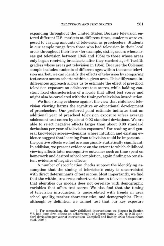
FIGURE ITelevision Penetration in 1950 and 1960 by Year of Television IntroductionSource. Television Factbook, various years; 1950 and 1960 U.S. Censuses.Notes. The height of each bar is the fraction of households with television sets
as recorded in the 1950 or 1960 census, averaged over all DMAs that receivedtelevision in the given year. Years in which no county received its first station areomitted from the figure.
To illustrate the impact of broadcast availability on televi-sion ownership, we compare our availability measure with dataon television ownership from the 1950 and 1960 U.S. Censuses.Figure I shows the share of households owning televisions as afunction of the year in which television broadcasts began in the
TELEVISION AND TEST SCORES 289
DMA. The first graph, which shows penetration in 1950, revealsa clear distinction between counties that had a station in theirDMA and those that did not. The average penetration in DMAswhose first station began broadcasting before 1950 ranges from8% in the 1949 group to over 35% in the 1941 group, whereas theaverage for groups getting television after 1950 never exceeds 1%.The second graph shows that, by 1960, differences in penetrationacross these DMAs had largely disappeared. Differences in thetiming of introduction of television into different areas thus hada large initial impact, but by 1960 most late-adopting DMAs hadcaught up to those that began receiving broadcasts early. Thesepatterns will be crucial to allowing us to identify the effect oftelevision using differences across birth cohorts within a DMA.
An examination of historical records suggests two potentialsources of endogeneity in the timing of television’s introductionto a market. First, the FCC sought to maximize the number ofpeople who could receive a commercial television signal. Condi-tional on the quality of existing coverage in a market, the FCCtherefore handled applications to begin broadcasting in order ofthe market’s total population (Television Digest 1953). Second,because a station’s profitability was determined largely by adver-tising revenue, which in turn depended on the spending powerof the market’s population, commercial interest in operating sta-tions in a given market was highly related to the market’s totalretail sales or income.
The data confirm the expected role of population and income.Early- and middle-adopting DMAs had, on average, five timeslarger populations and 24% larger per capita incomes than late-adopting DMAs. After controlling for log population and income,however, differences between early and late adopters appear muchmore idiosyncratic. Indeed, in regressions controlling for log pop-ulation and income, F-tests show no statistically significant re-lationship between television adoption category and percent highschool educated, median age, or percent nonwhite at the DMAlevel. (See the online appendix to this paper for details.) All of themodels we estimate below will control for DMA-level log popula-tion and income, so the parameters will be driven solely by vari-ation in the availability of television orthogonal to these two fac-tors.15 In Section V.C below, we show formally that the remaining
15. The patterns in Figure I are substantively unchanged if we measure pen-etration using the residual from a regression of penetration on log(income) andlog(population) at the DMA level.

290 QUARTERLY JOURNAL OF ECONOMICS
variation in television adoption timing is not systematically re-lated to student-level observables.
III.C. Childhood Exposure to Television
The data described above allow us to calculate the number ofyears of a given student’s early childhood in which television sig-nals were available. In order to make the magnitudes we measurein the analysis below more easily interpretable, we will also usedata on the rate at which television ownership actually diffusedamong households in each county. We will use the term televi-sion exposure to refer to the expected number of years a child’shousehold owned a television during the child’s preschool years.
To construct our measure of exposure, we collect annual dataon television penetration for U.S. counties. We combine the 1950and 1960 U.S. Census data mentioned above with data from in-dustry sources covering 1953 to 1959.16 For years with missingdata, we used a linear interpolation (or extrapolation) from thesurrounding years, with a transformation that restricts penetra-tion shares to fall between zero and one.17
We use these penetration data to compute the expected yearsof television exposure during ages two through six in each countyfor each Coleman Study cohort.18 For example, consider studentsin some county who were in grade 12 in 1965, the year of theColeman Study. Most students in this group were born in 1948.Suppose that television penetration in the county was 10% in 1950
16. We use data from Television magazine’s Market Book for the years 1954–1959 and separate county-level data from the Television Factbook for 1953. Thesesources combine information from the Advertising Research Foundation, A.C.Nielsen, NBC, and CBS, as well as television shipments data, to construct annualestimates of penetration by county. The correlation between Television’s county-level penetration estimates for 1959 and the U.S. Census counts for 1960 is ahighly statistically significant 0.64 (p< .0001). Given that Television did not yethave access to the Census reports when producing these figures, this correlationsuggests reasonably high reliability.
17. In particular, we computed the transformation log (penetration/(1−penetration)) and imputed missing values using a linear interpolation (or ex-trapolation) of this transformed measure. We then used the inverse function toretransform the imputed values to a 0–1 scale. This approach amounts to assum-ing that television diffusion follows an S-shaped logistic process in years withmissing data (Griliches, 1957).
18. In results not reported, we have also experimented with separate mea-sures of television exposure during ages 0 through 3 and ages 4 through 6. Inthe specifications where we find marginally significant evidence of positive effectsof television—reading and general knowledge—the effects tend to be larger forexposure at ages 4 through 6 than for exposure at ages 0 through 3 (althoughthese differences are not statistically significant and this pattern does not holdfor all tests). This finding is consistent with historical evidence that older childrenwatched more hours of television.

TELEVISION AND TEST SCORES 291
(age two), 11% in 1951 (age three), 12% in 1952 (age four), 13% in1953 (age five), and 14% in 1954 (age six). Then we calculate thetotal years of preschool television exposure for twelfth graders inthis county as (0.10 + 0.11 + 0.12 + 0.13 + 0.14) = 0.6.19
We have chosen to ignore ages below two because there isrelatively less information about viewing patterns in those ages.We restrict attention to ages six and below because by age sixalmost every student in our sample lived in a market in whichtelevision broadcasts were available.
Please see Table A.1 for summary statistics.
IV. IDENTIFICATION AND REDUCED-FORM EVIDENCE
IV.A. Identification
The key advance of this study relative to previous work isto identify the effect of television on test scores using variationacross local markets in the timing of television’s introduction. InAppendix I, we use the Coleman data to examine the potential bi-ases in an approach that uses cross-sectional correlations betweentelevision viewing and test scores, as is done in the bulk of theexisting literature. We show that virtually every observable char-acteristic in our data that is related to test scores is also stronglycorrelated with television viewing hours. Depending on which setof characteristics we include as controls, we can reproduce highlysignificant partial correlations of television and test scores thatare either positive or negative. This suggests that inferring causalrelationships from such correlations is a dubious enterprise.
To illustrate our approach to identification, suppose thatchildhood television viewing has a negative effect on test scores.Consider two cities, an early adopter where television was intro-duced in 1948, and a late adopter where it was introduced in1954. In the first city, sixth, ninth, and twelfth graders were allable to watch television throughout childhood (recall that twelfthgraders in the Coleman Study were born in 1948). In the secondcity, sixth graders had television available throughout their lives,but ninth graders only had access to it starting at age three andtwelfth graders only at age six. We would therefore expect twelfth
19. For those students for whom we know SMSA but not county, we computethe analogous measure at the SMSA level. Because our measure of televisionexposure is more precise for the 38% of students for whom the county is known,we have verified that our qualitative conclusions are robust to focusing only onthis subsample of students.

292 QUARTERLY JOURNAL OF ECONOMICS
graders in the second city to perform well relative to sixth andninth graders in that city, and ninth graders to perform slightlybetter than sixth graders. In the first city, we would expect nosuch pattern. By differencing out the mean test scores by gradefrom the first city, we could isolate the effects of television usinggrade patterns in the second city.
A simple way to implement this strategy would be to run a re-gression of test scores on the number of preschool years that tele-vision broadcasts were available in a student’s city, controlling forgrade and city fixed effects. Cities where television availability didnot vary across grades would identify the grade fixed effects; sixthgraders, for whom television was available throughout childhoodin essentially all cities, would identify the city fixed effects. Theremaining variation in the grade pattern of test scores betweencities would identify the parameter on years of availability.
Note that the interpretation of these results—denominated inyears of television broadcast availability rather than years a childactually had a television in his or her home—would differ greatlydepending on the speed at which television ownership diffused. Agiven effect of a year of television availability could reflect a largeeffect of exposure if few households actually adopted, or a muchsmaller effect if adoption was widespread.
In order to make the magnitudes of our coefficients moredirectly interpretable, we therefore wish to scale our estimatesusing data on television exposure, constructed as described inthe previous section. One way to do this would be to simply re-place availability with exposure on the right-hand side. But theseresults would be identified in part by variation in television pur-chase decisions—likely to be strongly correlated with county-levelunobservables—rather than by variation in the timing of televi-sion’s introduction. Instead, we adopt a two-stage least squares(2SLS) approach. We include exposure on the right-hand side butinstrument for it using data on the year in which television wasfirst introduced. This means that the model will be identifiedsolely by variation in the timing of television’s introduction, butthe magnitudes will be interpretable as the effect of a year ofactual television exposure.20
20. It also means that our estimates (and standard errors) will be consistenteven if we measure exposure with error, provided that the error is classical, in thesense of being independent across DMAs.

TELEVISION AND TEST SCORES 293
To state this approach more formally, let ygc be the averagetest scores of students in grade g in location c, measured as of1965. Given the geographic information included in the Colemandata, we will define a location to be either an SMSA or a county (forareas not in SMSAs). Let TVgc be the number of years of preschooltelevision exposure of the average student in grade g and locationc, constructed as described in Section III.C above. We can write
(1) ygc = βTVgc + φgWc + δc + γg + εgc,
where δc and γg are location and grade fixed effects, respectively,and εgc is a city-grade level error term, possibly correlated acrossgrades within a city.21
The term φgWc represents the DMA-level log population andlog income of a location Wc multiplied by a grade-specific coeffi-cient vector φg, where the population and income figures are takenfrom the 1960 Census. As discussed above, an examination of thehistorical record suggests that DMA population and income werethe most important observable predictors of the timing of televi-sion’s introduction. Although our identification strategy will relyonly on changes across cohorts within a given market (rather thandifferences across markets), including income and population con-trols (interacted with grade) will limit the chance that our resultswill be confounded by unobserved differences in cohort or timetrends across markets of different size or wealth.22
We instrument for TVgc with interactions between grade dum-mies and dummies for whether the city was an early, middle, orlate adopter of television. The first stage of this model can bewritten as
(2) TVgc = β0g ADOPTc + φ0
g Wc + δ0c + γ 0
g + ε0gc,
where ADOPTc is a vector of dummies indicating whether loca-tion c was an early, middle, or late adopter of television and β0
g is aseparate vector of parameters for each grade g. The instruments
21. Note that this model assumes that the effects of television depend onlyon television ownership, not on the number of viewing hours. Available data onchildren in television households show no obvious time trend in television hoursduring the early years of television (see Section II above). This suggests thatour instrument may not have had a first-order effect on hours watched, makingspecification in equation (1) a reasonable approximation.
22. Consistent with evidence that population and income capture the keydimensions of endogeneity in television timing, including additional DMA-levelcontrols interacted with grade (educational attainment, racial composition, me-dian age, and urbanization) does not meaningfully change our results.

294 QUARTERLY JOURNAL OF ECONOMICS
β0g ADOPTc capture the critical cross-city-cross-grade variation in
the availability of television that will identify the effect of expo-sure. The crucial identifying assumption in this model is that,conditional on the controls, the interaction between the timingof television introduction and the birth cohort of the student isorthogonal to the error term in equation (1). Under this assump-tion, our estimate of the parameter β in equation (1) will be in-terpretable as the causal effect of an additional year of preschooltelevision exposure on test scores.
Although our model can be estimated with aggregate dataalone, we wish to take advantage of the availability of theindividual-level data in the Coleman sample. This will allow usto include tighter controls for geography, in particular permittingthe use of school rather than location fixed effects. It will alsoallow us to control for characteristics of individual householdsand students that might affect exam performance. Both types ofinformation would be expected to improve precision. Of course,because the timing of television introduction is measured at theDMA level, in moving to microdata we must be careful to avoidaggregation bias (Moulton 1990). We will therefore cluster ourstandard errors at the DMA level, which will also account for anyserial correlation across different grades within the same DMA(Bertrand, Duflo, and Mullainathan 2004).23
In the next subsection, we present OLS estimates of the first-stage equation (2) and of the reduced-form second stage. In Sec-tion V we present 2SLS estimates of equation (1). We note thatthe latter estimates are necessarily local to the students whoseexposure to television was affected by the introduction of televi-sion (Angrist 2004) so that students in households whose decisionto adopt television was more responsive to broadcast availabilitywould implicitly receive more weight in our estimation. In SectionVI, we provide evidence on the heterogeneity in treatment effectsin the student population and discuss how this heterogeneity isrelated to television viewership rates.
IV.B. First-Stage and Reduced-Form Estimates
Before estimating model (1) formally, it will be helpful to ex-amine the variation that will identify it. In Figure II, we plot the
23. As expected, specifications in which we aggregate the Coleman test scoredata to the DMA level and then estimate our model at the aggregate level returnsimilar point estimates with larger standard errors.

TELEVISION AND TEST SCORES 295
0
0.05
0.1
0.15
0.2
0.25
0.3
0.35
1948
1949
1950
1951
1952
1953
1954
1955
1956
1957
1958
1959
1960
1961
Dif
fere
nce
in te
levi
sion
pen
etra
tion
12th-gradersborn
9th-gradersborn
6th-gradersborn
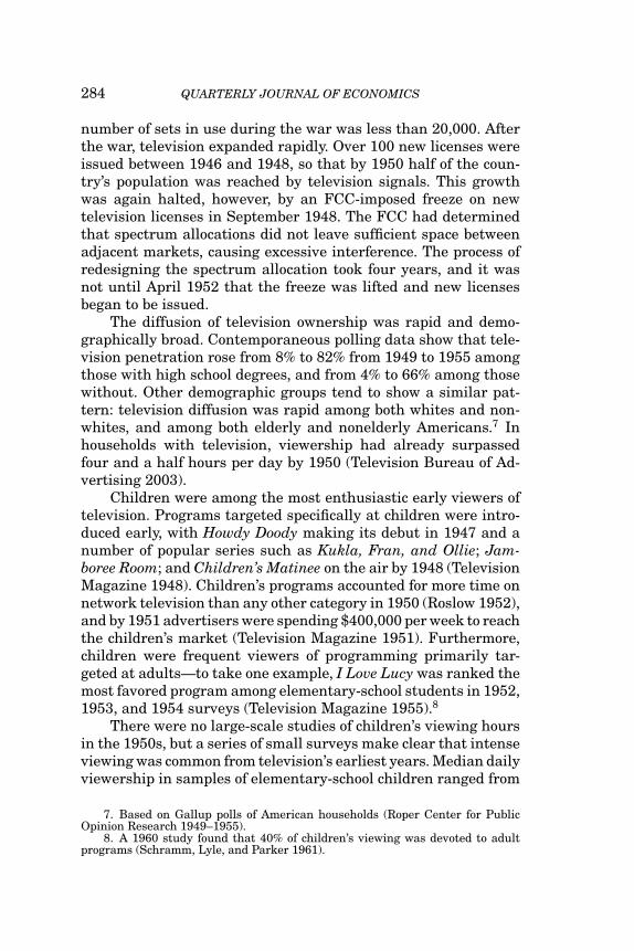
FIGURE IIDifference in Television Penetration between Early/Middle and Late Adopters
Source. Authors’ calculations.Notes. Figure is based on separate year-by-year regressions of television pen-
etration on a dummy for early/middle television adoption (television introduced1951 or earlier), log income, and log population. The values plotted are the coeffi-cients on the early/middle adoption dummy. The values thus represent the differ-ence in television penetration between early/middle adopters and late adopters ineach year, adjusted for differences in log income and log population.
coefficients from year-by-year regressions of DMA television pene-tration on a dummy for having received a television station before1952 (controlling for log population and log income). The figurethus shows how pre-1952 television introduction’s impact on pen-etration changes over time. During the period from 1948 to 1954,when the twelfth graders in the Coleman sample were of preschoolage, television penetration was substantially higher in early- andmiddle-adopting DMAs than in late-adopting DMAs. By contrast,in the post-1954 period, when the sixth graders in the sample werepreschoolers, the late adopters (most of which received televisionby 1954) had largely caught up to the early and middle adopters.In other words, differences in adoption dates across DMAs hadthe largest impact on television exposure for the twelfth gradersin the sample, a smaller impact on the ninth graders, and only aminimal impact on the sixth graders. This interaction between astudent’s grade and the impact of the timing of television intro-duction is what will allow us to estimate the effect of televisionexposure on test scores.

296 QUARTERLY JOURNAL OF ECONOMICS
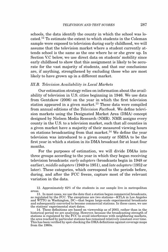
Turning to formal estimation, column (1) of Table I presentsestimates of the first stage of our model, regressing TVgc on inter-actions between grade dummies and dummies for whether the citywas an early, middle, or late adopter of television. Observe firstthat, for a given grade, television exposure was lower the latertelevision was introduced to the student’s city. So, for example,students in grade nine whose DMAs adopted late were exposed totelevision for about 0.8 years less than ninth graders whose DMAsadopted early, and about 0.5 years less than those whose DMAswere middle adopters. A similar pattern is present for students ingrade 12.
Next, note that, holding constant the timing of television’sintroduction to a market, twelfth graders on average had lesspreschool television exposure (between the ages of 2 and 6) thanninth graders, and much less than sixth graders (the omittedcategory). For example, twelfth graders in late-adopting DMAshad television in their homes for about 1.1 years less than sixthgraders in these same DMAs, and about 0.3 years less than ninthgraders. This is what we would expect because twelfth graderswere born in 1948, ninth graders were born in 1951, and sixthgraders were born in 1954. So in cities receiving television af-ter 1948, ninth graders were more likely than twelfth graders tospend their preschool years in a city in which a television sig-nal was available, and sixth graders were almost certain to havegrown up with a television in the household.
These findings complement the evidence in Figure I in show-ing that the timing of broadcast availability had a substantialimpact on television penetration and hence on students’ exposureto television as young children. Each of the grade-timing inter-action terms is strongly individually significant, and the F-testpresented in Table I definitively rejects the null hypothesis thatthese interactions have no impact on exposure.24
In column (2), we present a reduced-form second-stage es-timate of the effect of our instruments on test scores. We useas our dependent variable the average of the student’s (stan-dardized) scores on the math, reading, verbal, and spatial rea-soning tests. If television exposure exerted a negative long-termeffect on cognitive skills, we would expect the coefficients on thegrade-timing interactions in column (2) to move inversely with
24. The F-statistic in this first-stage model is sufficient to rule out any sizableweak instruments bias (Stock and Yogo 2002).

TELEVISION AND TEST SCORES 297T
AB
LE
IR
ED
UC
ED
-FO
RM
ES
TIM
AT
ES
OF
TH
EE
FF
EC
TO
FP
RE
SC
HO
OL
TE
LE
VIS
ION
EX
PO
SU
RE
ON
AD
OL
ES
CE
NT
TE
ST
SC
OR
ES
Sta
nda
rdiz
edav
erag
eN
um
ber
ofye
ars
ofte
stsc
ore
Cu
rren
tte
levi
sion
expo
sure
view
ing
hou
rs(1
)(2
)(3
)(4
)(5
)
DM
Ais
mid
dle
adop
ter
(TV
in19
49–1
951)
×G
rade
9−0
.262
4−0
.022
9−0
.000
2−0
.007
60.
0527
(0.0
840)
(0.0
439)
(0.0
296)
(0.0
290)
(0.0
372)
×G
rade
12−0
.713
7−0
.048
0−0
.031
2−0
.034
70.
0853
(0.1
626)
(0.0
477)
(0.0
343)
(0.0
319)
(0.0
560)
DM
Ais
late
adop
ter
(TV
in19
52or
late
r)×
Gra
de9
−0.7
641
−0.0
066
0.00
33−0
.007
7−0
.008
1(0
.106
9)(0
.044
3)(0
.033
3)(0
.033
8)(0
.043
8)×
Gra
de12
−1.0
862
0.00
170.
0001
−0.0
140
0.05
36(0
.283
1)(0
.049
3)(0
.039
3)(0
.037
1)(0
.068
7)S
choo
lan
dgr
ade
fixe
def
fect
s?Y
ES
YE
SY
ES
YE
SY
ES
DM
Ade
mog
raph
ics
×gr
ade?
YE
SY
ES
YE
SY
ES
YE
SS
tude
nt
dem
ogra
phic
s?N
ON
OY
ES
YE
SY
ES
Dem
ogra
phic
s×
grad
e?N
ON
ON
OY
ES
YE
SF
(4,13
5)st
aton
inst
rum
ents
16.5
80.
910.
790.
611.
44(p
-val
ue)
(<.0
001)
.462
8.5
334
.653
7.2
229
Nu
mbe
rof
obse
rvat
ion
s34
6,56
234
6,56
234
6,56
234
6,56
233
5,98
1N
um
ber
ofsc
hoo
ls80
080
080
080
080
0N
um
ber
ofD
MA
s13
613
613
613
613
6
Sou
rce.
Au
thor
s’ca
lcu
lati
ons
base
don
Col
eman
Stu
dyda
ta.
Not
es.S
tan
dard
erro
rsin
pare
nth
eses
are
adju
sted
for
clu
ster
ing
onD
MA
.DM
Ade
mog
raph
ics
incl
ude
log(
DM
Apo
pula
tion
)in
1960
and
log(
DM
Ato
tali
nco
me)
in19
59.S
tude
nt
dem
ogra
phic
sin
clu
des
con
trol
sfo
rge
nde
r,E
ngl
ish
spok
enat
hom
e,fa
ther
’sed
uca
tion
,mot
her
’sed
uca
tion
,rac
e,li
ves
wit
hbi
olog
ical
fath
er,l
ives
wit
hbi
olog
ical
mot
her
,an
dse
para
tedu
mm
ies
for
wh
eth
erst
ude
nt’s
fam
ily
has
ate
leph
one,
are
cord
play
er,a
refr
iger
ator
,ava
cuu
mcl
ean
er,o
ra
car.
Du
mm
ies
are
incl
ude
dto
indi
cate
mis
sin
gva
lues
for
dem
ogra
phic
con
trol
s.T
he
depe
nde
nt
vari
able
inco
lum
n(5
)is
the
repo
rted
aver
age
nu
mbe
rof
dail
yte
levi
sion
view
ing
hou
rsat
the
tim
eof
the
Col
eman
stu
dy(1
965)
.

298 QUARTERLY JOURNAL OF ECONOMICS
the coefficients in column (1). In other words, we would expect thestudents who had relatively less childhood television exposureto perform better on standardized tests. As the column shows,however, we do not see such a pattern. Although students frommiddle-adopting DMAs perform slightly better than those fromlate-adopting DMAs, these students perform worse than thosefrom early-adopting DMAs. Additionally, among students frommiddle-adopting DMAs, twelfth graders perform worse than ninthgraders and sixth graders, despite having spent more time with-out television in their households.
An F-test of the null hypothesis that the grade–timing inter-actions had no effect on test scores fails to reject at conventionalsignificance levels. Adding demographic controls in columns (3)and (4) improves the precision of our estimates by explaining alarger share of the variation in test scores. These more preciseestimates show even less evidence of a negative effect of televi-sion. In column (4), where our standard errors are lowest, we findsmall point estimates on nearly all interaction terms, and the dif-ferences among these coefficients do not support the hypothesis ofa negative effect of television on test scores.
Finally, in column (5), we present reduced-form second-stageestimates of the effect of our instruments on the number of hoursof contemporaneous (1965) television viewing. The grade–timinginteractions are both individually and jointly insignificant. Thisconfirms that our estimates will capture the effect of lagged ratherthan contemporaneous exposure.
V. TELEVISION AND COGNITIVE DEVELOPMENT
V.A. Two-Stage Least Squares (2SLS) Estimates
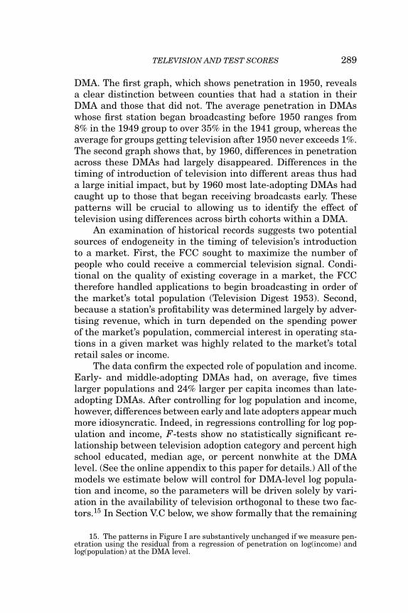
In Table II, we present estimates of equation (1) computedusing 2SLS. Coefficients in these models can be interpreted asthe causal effect of a year of preschool television exposure on testscores.
We present results for the average test score as well asfor each individual component score. For each test, we presentbaseline estimates, estimates with demographic controls, and es-timates with demographics interacted with a student’s grade.Adding controls should improve the precision of our estimatesby leaving a smaller share of the overall variation in test scoresunexplained.

TELEVISION AND TEST SCORES 299
TA
BL
EII
ST
RU
CT
UR
AL
(2S
LS
)E
ST
IMA
TE
SO
FT
HE
EF
FE
CT
OF
PR
ES
CH
OO
LT
EL
EV
ISIO
NE
XP
OS
UR
EO
NA
DO
LE
SC
EN
TT
ES
TS
CO
RE
S
Sta
nda
rdiz
edco
mpo
nen
tS
tan
dard
ized
aver
age
Spa
tial
Gen
eral
test
scor
eM
ath
reas
onin
gV
erba
lR
eadi
ng
know
ledg
e
Eff
ect
ofn
um
ber
ofye
ars
ofpr
esch
oolt
elev
isio
nex
posu
reB
asel
ine
0.01
29−0
.019
2−0
.007
10.
0268
0.04
700.
0466
(0.0
384)
(0.0
440)
(0.0
480)
(0.0
404)
(0.0
347)
(0.0
491)
Bas
elin
e+
dem
ogra
phic
s0.
0140
−0.0
154
−0.0
046
0.02
540.
0461
0.06
77(0
.030
8)(0
.037
6)(0
.045
7)(0
.029
4)(0
.029
5)(0
.040
8)B
asel
ine
+de
mog
raph
ics
×gr
ade
0.02
25−0
.017
90.
0028
0.02
940.
0557
0.06
72(0
.027
9)(0
.037
8)(0
.038
7)(0
.028
9)(0
.030
2)(0
.041
0)N
um
ber
ofob
serv
atio
ns
346,
562
346,
562
346,
562
346,
562
346,
562
226,
487
Nu
mbe
rof
sch
ools
800
800
800
800
800
705
Nu
mbe
rof
DM
As
136
136
136
136
136
134
Sou
rce.
Au
thor
s’ca
lcu
lati
ons
base
don
Col
eman
Stu
dyda
ta.
Not
es.
Est
imat
esar
efr
om2S
LS
mod
els
wit
hin
tera
ctio
ns
betw
een
grad
ean
dca
tego
ryof
tele
visi
onin
trod
uct
ion
year
use
das
inst
rum
ents
for
year
sof
tele
visi
onex
posu
re.
Sta
nda
rder
rors
inpa
ren
thes
esar
ead
just
edfo
rcl
ust
erin
gon
DM
A.
All
depe
nde
nt
mea
sure
sar
est
anda
rdiz
edto
hav
ea
mea
nof
zero
and
ast
anda
rdde
viat
ion
ofu
nit
yw
ith
inea
chgr
ade.
Bas
elin
ein
clu
des
fixe
def
fect
sfo
rsc
hoo
lan
dgr
ade
and
inte
ract
ion
sbe
twee
ngr
ade
and
log(
DM
Apo
pula
tion
)in
1960
and
log(
DM
Ato
tali
nco
me)
in19
59.D
emog
raph
ics
incl
ude
sco
ntr
ols
for
gen
der,
En
glis
hsp
oken
ath
ome,
fath
er’s
edu
cati
on,
mot
her
’sed
uca
tion
,ra
ce,
live
sw
ith
biol
ogic
alfa
ther
,li
ves
wit
hbi
olog
ical
mot
her
,an
dse
para
tedu
mm
ies
for
wh
eth
erst
ude
nt’s
fam
ily
has
ate
leph
one,
are
cord
play
er,a
refr
iger
ator
,ava
cuu
mcl
ean
er,o
ra
car.
Du
mm
ies
are
incl
ude
dto
indi
cate
mis
sin
gva
lues
for
dem
ogra
phic
con
trol
s.G
ener
alkn
owle
dge
test
scor
esar
eav
aila
ble
only
for
stu
den
tsin
grad
es9
and
12.

300 QUARTERLY JOURNAL OF ECONOMICS
The first column shows our estimates of the effect of an ad-ditional year of television exposure on the student’s average testscore, expressed in units of standard deviations (by grade). Ingeneral, we find small, statistically insignificant, and positive esti-mates, suggesting that, if anything, childhood television exposureimproves a student’s test scores. Adding controls tends to increasethe point estimates and, consistent with expectations, decreasethe standard errors of these estimates. In the final specificationwith demographic controls interacted with grade dummies, we areable to reject negative effects of television larger than about 0.03standard deviations per year of exposure.25
The remaining columns present the estimated effect of tele-vision on test scores in each subject separately. In no case dowe see clear evidence for a negative effect of television. Column(2) shows that the effects on mathematics and spatial reasoningrange from slightly negative to slightly positive and are in allcases statistically insignificant. With our largest set of controls,we find point estimates of −0.018 and 0.003 standard deviationsper year of television exposure for mathematics and spatial rea-soning respectively. Our point estimates on verbal and readingscores are always positive, with the effect on reading scores amarginally statistically significant 0.06 standard deviations inthe final specification (p = .065). This in turn means that we canrule out even very small negative effects—our confidence intervalin this specification excludes a negative effect on reading scoresof about 0.004 standard deviations. Finally, the preferred pointestimate for the effect on general knowledge is a positive effect ofabout 0.07 standard deviations per year of television exposure.
Although we are reluctant to draw firm conclusions from thecomparison of coefficients across test scores, we note that the pat-tern of relatively positive effects on verbal, reading, and generalknowledge scores is consistent with a variety of existing evidencesuggesting that children can learn language-based skills fromtelevision. For example, Rice (1983) argues that the presenta-tion of verbal information on television is especially conducive tolearning by young children. Rice and Woodsmall (1988) presentlaboratory evidence that children aged three and five can learn
25. Because we have multiple instruments, we can perform a test of over-identifying restrictions as an additional check on the validity of the instruments.A test using Hansen’s J-statistic (Hansen 1982; Hoxby and Paserman 1998; Baum,Schaffer, and Stillman 2003) cannot reject the null hypothesis that the instrumentsare uncorrelated with the error term (J = 1.928, p = .5874).

TELEVISION AND TEST SCORES 301
unfamiliar words from watching television. The effect on generalknowledge scores might also reflect the fact that television alsoexposes young children to a large number of facts, some of whichmight be retained into adolescence.26
V.B. Interpretation of Magnitudes
To provide a better sense of the magnitudes of our coefficientsand standard errors, we can contrast them with experimental find-ings in which children exposed to an intervention as preschoolersare followed into adolescence. Perhaps the two best-known in-stances of such experiments are the Perry Preschool Study andthe Carolina Abecedarian Project (Campbell and Ramey 1995;Schweinhart et al. 2005).27 Both studies focused on children fromrelatively poor families. The Perry study enrolled an interven-tion group in a two-year part-day preschool education programduring ages three and four. The Abecedarian project enrolled chil-dren in a five-year full-day day care program through age five. Inboth cases, children were randomly assigned to intervention andcontrol conditions, and both sets of children were followed intoadolescence. In the Perry program, children in the interventiongroup scored one- to two-thirds of a standard deviation higher onachievement tests at age fourteen (the average age of studentsin our Coleman sample), with an overall effect of about one-halfof a standard deviation. In the Abecedarian program, effect sizeson achievement at age fifteen were on the order of one-third ofa standard deviation. Norming these effects for the differencesin treatment duration between the studies, the Perry programhad an impact on achievement of approximately 0.25 standarddeviations per year of intervention, and the Abecedarian programhad an impact of approximately 0.07 to 0.08 standard deviations
26. The fact that television exposure improves factual knowledge may alsopartly explain its effect on reading scores because some evidence indicates thatbackground knowledge can improve reading comprehension (Langer 1984), at leastif it is consistent with the information in the test passage (Alvermann, Smith, andReadence 1985).
27. These are the only two randomized studies receiving detailed attention inCunha et al.’s (2006) review. Currie’s (2001) review identifies two other randomizedpreschool interventions with long-term follow-up data: the Milwaukee Project andthe Early Training Project. The Milwaukee Project offered a five-year full-day daycare program through age 5, along with job and academic training for mothers. Asof grade 8, the study had an effect of about two-thirds of a standard deviation onIQ (more than 0.1 standard deviations per intervention year) but no statisticallysignificant effect on achievement test scores (Barnett 1995). The Early TrainingProject, which involved a much less intensive intervention, substantially reducedspecial education participation in the long term, and had positive, though notstatistically significant, long-term effects on student achievement (Currie 2001).

302 QUARTERLY JOURNAL OF ECONOMICS
per year.28 The long-term effects of these preschool interventionstherefore tend to exceed effects on the order of the low end of ourmain confidence interval (about 0.03 standard deviations per yearof television).
V.C. Specification Checks
Are the Instruments Correlated with Student Characteristics?The models presented above are valid under the assumption
that our instruments—interactions between the timing of televi-sion introduction and grade—are orthogonal to the error term.Of course, it is by definition impossible to test this assumption.Some relevant information, however, can be obtained by askingwhether television exposure is correlated with trends in observ-able demographic characteristics. Although the absence of such acorrelation is not proof of the identifying assumption, it does pro-vide some confidence that unobserved heterogeneity is unlikely tobias our estimates of the effect of television.
There are two related possibilities we wish to test for. Thefirst is that, in 1965, cross-grade differences in the householdcharacteristics of students within an area are correlated with thetiming of television’s introduction. The second is that demographictrends during the 1950s are correlated with the timing of televi-sion’s introduction, resulting in a relationship between a student’spreschool television exposure and the local circumstances duringhis or her upbringing.
To conduct a test for the first possibility, we use the first-stagemodel (2) to create a predicted number of years of television ex-posure for each student. By regressing this predicted value on aset of demographic characteristics, we can test whether the vari-ation in television exposure that is due to the timing of televisionintroduction is correlated with cross-grade differences in observ-able student characteristics that might be expected to affect testscores.
The results of this test are presented in Table III. Noneof the demographics has a statistically significant correlationwith predicted television exposure. Additionally, an F-test of thejoint hypothesis that none of the demographic characteristics is
28. Additional calculations based on program details imply that the Perryand Abecedarian programs had effects of approximately 0.22 and 0.01 standarddeviations per hour-year, respectively. A similar calculation assuming averageearly-childhood viewing of 1.5 hours per day puts the top end of the confidenceinterval for our television effects at about 0.02 standard deviations per hour-year.

TELEVISION AND TEST SCORES 303
TABLE IIIIS PREDICTED TELEVISION EXPOSURE CORRELATED WITH OBSERVABLES?
Predicted years of Standardized averagetelevision exposure test score
(1) (2)
Male −0.00087 −0.0589(0.00090) (0.0077)
English not spoken at home 0.00152 −0.2046(0.00100) (0.0088)
Father’s education (index) −0.00024 0.0622(0.00031) (0.0018)
Mother’s education (index) −0.00009 0.0551(0.00029) (0.0017)
White 0.00184 0.4400(0.00209) (0.0334)
Lives with biological father −0.00104 0.0862(0.00063) (0.0065)
Lives with biological mother 0.00003 0.1992(0.00092) (0.0068)
Family hasTelephone 0.00198 0.1215
(0.00203) (0.0090)Record player 0.00082 0.0246
(0.00077) (0.0050)Refrigerator −0.00074 0.4555
(0.00206) (0.0161)Vacuum 0.00105 0.0696
(0.00094) (0.0104)Car 0.00062 0.0677
(0.00081) (0.0105)F(12, 135) 1.41 705.63(p-value) (.1704) (<.0001)Number of observations 346,562 346,562Number of schools 800 800Number of DMAs 136 136
Source. Authors’ calculations based on Coleman Study data.Notes. Standard errors in parentheses are adjusted for clustering on DMA. Average test score is standard-
ized to have a mean of zero and a standard deviation of unity within each grade. All regressions include fixedeffects for school and grade and interactions between grade and log(DMA population) in 1960 and log(DMAtotal income) in 1959. Dummies are included to indicate missing values for demographic controls.
correlated with years of television exposure fails to reject (p =.170). Thus we find no evidence of a correlation between the lo-cal availability of television and observable characteristics, oncewe control for DMA-level population and income. This is true de-spite the fact that, as Table III also shows, these demographic

304 QUARTERLY JOURNAL OF ECONOMICS
characteristics are in most cases strong predictors of testscores.29
To test for a bias from differences in time trends in demo-graphics, we have also tested for a relationship between the timingof the introduction of television and changes in income, populationdensity, and adult schooling levels by DMA in the 1950s (see theonline appendix for details). We find no statistically significantrelationship and no consistent direction of correlation, lendingfurther support to the validity of our identifying assumption.
Are the Instruments Correlated with Teacher Characteristicsor School Resources?
Another possibility is that differences in school resources orteacher quality across cohorts are correlated with television entry.Here, again, we must check both for differences in resources at thetime of the Coleman Study and different trends in school qualityover time.
To check whether contemporaneous (1965) differences inteacher characteristics across grades are correlated with the yearof introduction of television, we take advantage of the fact thatthe Coleman Study collected a set of teacher surveys in addi-tion to student surveys and test scores. Using these, we estimatea regression of predicted television exposure by DMA-grade onthe average characteristics of teachers who taught in that gradein 1965. (See the online appendix for details.) Only one of theteacher characteristics (number of subjects taught) is statisticallysignificantly related to predicted television exposure in that grade(p = .040). An F-test of the joint significance of the twelve teachercharacteristics fails to reject at conventional significance levels(p = .111). Additionally, the signs of the coefficients suggest noclear pattern of more resources being associated with greater orlesser television exposure, again supporting the view that therewere no systematic cross-grade trends in teacher quality that werecorrelated with the timing of the introduction of television.30
29. Results are quite similar when we conduct the test on collapsed, DMA-grade-level data: an F-test does not reject the null hypothesis that predicted ex-posure is uncorrelated with student characteristics (p = .371). We have also con-ducted a parallel exercise (in the spirit of Altonji, Elder, and Taber 2005) in whichwe predict each student’s average test score using her demographics and then usethis predicted measure as the dependent variable in 2SLS analysis parallelingTable II. In this case, we again find no evidence of any correlation between ourinstruments and the demographic predictors of test scores.
30. Consistent with the conclusion that cross-grade variation in teacher char-acteristics is unrelated to the timing of television’s introduction to local areas, we
TELEVISION AND TEST SCORES 305
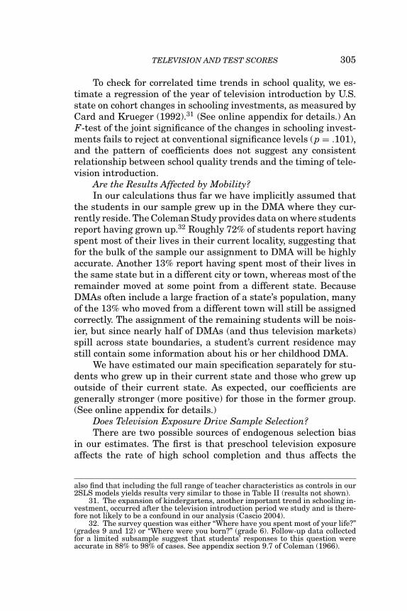
To check for correlated time trends in school quality, we es-timate a regression of the year of television introduction by U.S.state on cohort changes in schooling investments, as measured byCard and Krueger (1992).31 (See online appendix for details.) AnF-test of the joint significance of the changes in schooling invest-ments fails to reject at conventional significance levels (p = .101),and the pattern of coefficients does not suggest any consistentrelationship between school quality trends and the timing of tele-vision introduction.
Are the Results Affected by Mobility?In our calculations thus far we have implicitly assumed that
the students in our sample grew up in the DMA where they cur-rently reside. The Coleman Study provides data on where studentsreport having grown up.32 Roughly 72% of students report havingspent most of their lives in their current locality, suggesting thatfor the bulk of the sample our assignment to DMA will be highlyaccurate. Another 13% report having spent most of their lives inthe same state but in a different city or town, whereas most of theremainder moved at some point from a different state. BecauseDMAs often include a large fraction of a state’s population, manyof the 13% who moved from a different town will still be assignedcorrectly. The assignment of the remaining students will be nois-ier, but since nearly half of DMAs (and thus television markets)spill across state boundaries, a student’s current residence maystill contain some information about his or her childhood DMA.
We have estimated our main specification separately for stu-dents who grew up in their current state and those who grew upoutside of their current state. As expected, our coefficients aregenerally stronger (more positive) for those in the former group.(See online appendix for details.)
Does Television Exposure Drive Sample Selection?There are two possible sources of endogenous selection bias
in our estimates. The first is that preschool television exposureaffects the rate of high school completion and thus affects the
also find that including the full range of teacher characteristics as controls in our2SLS models yields results very similar to those in Table II (results not shown).
31. The expansion of kindergartens, another important trend in schooling in-vestment, occurred after the television introduction period we study and is there-fore not likely to be a confound in our analysis (Cascio 2004).
32. The survey question was either “Where have you spent most of your life?”(grades 9 and 12) or “Where were you born?” (grade 6). Follow-up data collectedfor a limited subsample suggest that students’ responses to this question wereaccurate in 88% to 98% of cases. See appendix section 9.7 of Coleman (1966).

306 QUARTERLY JOURNAL OF ECONOMICS
composition of students who appear in the twelfth grade portionof the Coleman sample. The second is that television exposureaffects participation in the Coleman study conditional on beingenrolled in school, say, because of effects on attendance.
The evidence in Table III (discussed above) speaks to both ofthese concerns. It shows that observable correlates of test scoresappear to be balanced with respect to preschool television expo-sure. If television exposure changed the distribution of test scoresconditional on selecting into the Coleman sample, we would ex-pect it to affect the conditional distribution of other observablecharacteristics as well. For example, if exposure caused more low-achieving students to drop out of school between the ninth andtwelfth grades, we would expect to see relatively fewer twelfthgraders with low test scores in high-exposure areas. However, wewould expect to see relatively fewer twelfth graders with low fam-ily income and parental education as well. The fact that we do notsee this pattern suggests that selection is unlikely to be biasingthe results.
To more directly address the possibility that television ex-posure affects dropout rates, we use Census microdata to studythe effect of television exposure on high school completion (seeonline appendix for details). There is no evidence that preschooltelevision exposure affects the likelihood of having completed highschool as of adulthood although we note that the precision of theseestimates is lower than the precision of estimates based on theColeman data.
We have also reestimated our models excluding twelfthgraders who are most likely to have selectively dropped out ofschool prior to surveying (results not shown). As expected, thestandard errors of our models increase due to the exclusion of alarge portion of the data, but the resulting regressions continueto show no evidence of negative effects of television.
Finally, to investigate effects of television on selection intothe pool of Coleman test takers, we have compared the numberof students in the Coleman sample with the number we wouldpredict based on principals’ reports of school sizes (in the spiritof Jencks [1972]). We find no evidence that television exposureaffected rates of inclusion in the Coleman sample.
V.D. Television and Noncognitive Outcomes
The analysis above addresses the effect of television viewingon cognitive development. But it may be that many of television’s

TELEVISION AND TEST SCORES 307
TABLE IVEFFECT OF PRESCHOOL TELEVISION EXPOSURE ON ADOLESCENT SOCIAL AND
BEHAVIORAL OUTCOMES
Effect of one year ofDependent variable television exposure N
Number of hours spent on homework each day 0.0148 334,717(0.0422)
Number of books read during summer (standardized) −0.0760 336,127(0.0422)
Student sometimes feels like (s)he “just can’t learn” −0.0040 327,281(0.0208)
Highest grade student wants to finish in school −0.0265 333,570(standardized) (0.0221)
Share of membership organizations 0.0170 217,392(0.0398)
Source. Authors’ calculations based on Coleman Study data.Notes. Estimates are from 2SLS models with interactions between grade and category of television
introduction year used as instruments for years of television exposure. Standard errors in parentheses areadjusted for clustering on DMA. Standardized measures have a mean of zero and a standard deviation ofunity within each grade. Baseline includes fixed effects for school and grade and interactions between gradeand log(DMA population) in 1960 and log(DMA total income) in 1959. All regressions include controls forgender, English spoken at home, father’s education, mother’s education, race, lives with biological father,lives with biological mother, and separate dummies for whether student’s family has a telephone, a recordplayer, a refrigerator, a vacuum cleaner, or a car, as well as for interactions between grade dummies and thesecontrols. Dummies are included to indicate missing values for demographic controls. Share of membershiporganizations is number of the following organizations that the student belongs to, divided by the total numberof organizations for which the student provides a response: sports team, Student Council, debate team, andhobby club. Participation in membership organizations is available only for students in grades 9 and 12.
most important effects are on noncognitive traits.33 We can usethe Coleman data to estimate the effect of early childhood televi-sion exposure on several social and behavioral outcomes in lateryears. We note that, as with the previous analysis, our data donot permit us to say anything about the effect of television oncontemporaneous noncognitive outcomes. Table IV reports 2SLSestimates of the effect of preschool television exposure on severaladolescent attitudinal and behavioral outcomes. The effects aremostly small, negative, and statistically insignificant. The mainexception is a marginally statistically significant negative effecton the number of books a student reads during the summer. Wealso find a statistically insignificant and small positive effect onthe number of hours the student spends on homework each day.
We have also used data from the Integrated Public Use Mi-crodata Series (Ruggles et al. 2004) to test for effects of televisionon long-run labor market outcomes. We extracted information on
33. See, for example, Heckman and Rubinstein (2001) for evidence of theeconomic value of noncognitive skills.

308 QUARTERLY JOURNAL OF ECONOMICS
schooling attainment and wages for cohorts born in 1948, 1951,and 1954 from the 1970, 1980, 1990, and 2000 1% samples ofthe Census. Information on state of birth provides a coarse mea-sure of the geographic area in which individuals lived in earlychildhood, allowing us to apply a similar identification strategy toestimate the causal impact of television. The results show no evi-dence of a negative effect of television, although the coarseness ofthe geographic identifiers means that the precision of these esti-mates is limited. Details of this exercise are available in our onlineappendix.
VI. HETEROGENEITY IN THE EFFECTS OF TELEVISION
Our results thus far focus on the effect of preschool televisionexposure on the test scores of the average student in our dataset.For many purposes, however, it will be important to know howthe effects of television are distributed in the population, espe-cially with respect to the socioeconomic status of the student’shousehold. A body of evidence from developmental psychologyshows that the in-home learning environment is richer in higher-socioeconomic-status households, especially with respect to lan-guage and vocabulary (Hart and Risley 1995, 1999). Embeddedin a simple time-allocation framework (Becker 1965), this evi-dence would lead one to expect that television is more beneficialto children from more disadvantaged backgrounds, because forsuch children the activities crowded out by television are likely tobe less cognitively stimulating.34 Of course, this prediction couldchange if richer or more educated parents were better able toselect educational programming for their children to watch.35
In this section, we offer evidence on the question of whichchildren benefit the most (or are harmed the least) from televisionexposure. On the whole, our findings support the prediction thattelevision is most beneficial to children in households with theleast parental human capital.
34. The distinction between the direct effect of television content on the viewerand the indirect effect working through displacement of other activities is dis-cussed by Gaddy (1986) and Beentjes and Van der Voort (1988), among others.
35. The evidence we are aware of does not consistently support the viewthat more educated parents invest more in controlling programming. Rossiter andRobertson (1975) find no evidence of greater supervision by more educated parents,and Pinon, Huston, and Wright (1989) find no relationship between parental edu-cation and children’s viewing of educational television. One possible explanationis that education also raises parents’ opportunity cost of time.

TELEVISION AND TEST SCORES 309
In Table V, we present a first look at heterogeneous effectsby splitting the sample along several salient demographic dimen-sions. The first two columns repeat our basic 2SLS specificationfor students whose mothers do and do not have a high school ed-ucation.36 The estimated effect of a year of television exposure onthe average test score is 0.04 for students whose mothers haveless than a high school education, and 0.01 for students whosemothers have a high school degree. A similar pattern is presentfor individual test scores.
The next two columns compare households where Englishwas and was not the primary language. The estimated effectsof television on verbal, reading, and general knowledge scoresfor students in non-English-speaking households are positive andnontrivial in magnitude. For the sample of students whose familymembers primarily speak English, the point estimates are stillpositive but are much smaller. The point estimates for math andspatial reasoning also suggest more positive effects for studentsin non-English-speaking households.
In the final two columns, we present results for white andnonwhite students. We find that nonwhite students benefit con-siderably more from television exposure than do white students.The point estimate of the effect on average test scores is morethan 0.05 for nonwhite students, as compared to less than 0.01 forwhite students.
To combine the information from these various subsamplecomparisons, we take advantage of a question in the ColemanStudy survey that asks students how often they were read to athome prior to starting school. The possible responses range from“never” to “regularly.” We anticipate that this measure will becorrelated with the overall amount of “quality” time parents spendwith their children, and so we treat it as a broad proxy for parentalinvestment. Because parental reading may be directly affectedby the availability of television and may also be measured witherror,37 we will not use the measure directly but instead use thepredicted level as a function of demographics. This will combinevariation in parental education, English knowledge, race, and soforth into a single summary measure of parental investment.
36. We obtain similar results using father’s education to split the samplerather than mother’s education.
37. Response agreement between children and their parents on the questionof preschool reading ranged from 60% to 80%, depending on the student’s grade(Coleman 1966).

310 QUARTERLY JOURNAL OF ECONOMICST
AB
LE
VH
ET
ER
OG
EN
EIT
YIN
TH
EE
FF
EC
TS
OF
PR
ES
CH
OO
LT
EL
EV
ISIO
NE
XP
OS
UR
EO
NA
DO
LE
SC
EN
TT
ES
TS
CO
RE
S
Mot
her
has
HS
degr
ee?
En
glis
hat
hom
e?W
hit
e?
Yes
No
Yes
No
Yes
No
(1)
(2)
(3)
(4)
(5)
(6)
Eff
ect
ofn
um
ber
ofye
ars
ofpr
esch
oolt
elev
isio
nex
posu
reon
Ave
rage
scor
e0.
0135
0.04
180.
0157
0.07
660.
0026
0.05
26(0
.029
7)(0
.033
4)(0
.027
7)(0
.047
9)(0
.026
2)(0
.048
9)M
ath
−0.0
477
0.02
89−0
.028
30.
0352
−0.0
293
−0.0
055
(0.0
422)
(0.0
354)
(0.0
390)
(0.0
476)
(0.0
405)
(0.0
445)
Spa
tial
reas
onin
g0.
0125
−0.0
342
−0.0
050
0.05
920.
0225
−0.0
345
(0.0
395)
(0.0
446)
(0.0
362)
(0.0
608)
(0.0
277)
(0.0
577)
Ver
bal
0.03
080.
0482
0.02
520.
0740
−0.0
191
0.11
67(0
.029
4)(0
.039
8)(0
.028
5)(0
.052
9)(0
.018
9)(0
.047
1)R
eadi
ng
0.04
500.
0942
0.05
280.
0927
0.02
730.
0922
(0.0
316)
(0.0
454)
(0.0
332)
(0.0
453)
(0.0
386)
(0.0
543)
Gen
eral
know
ledg
e0.
0074
0.06
570.
0260
0.21
23−0
.094
50.
1401
(0.0
529)
(0.0
487)
(0.0
378)
(0.1
551)
(0.0
423)
(0.0
786)
Nu
mbe
rof
obse
rvat
ion
sA
llgr
ades
157,
788
112,
849
280,
455
57,5
1421
1,58
012
6,88
6G
rade
s9
and
1211
0,80
582
,874
186,
126
36,1
9614
2,32
879
,713
Sou
rce.
Au
thor
s’ca
lcu
lati
ons
base
don
Col
eman
Stu
dyda
ta.
Not
es.
Est
imat
esar
efr
om2S
LS
mod
els
wit
hin
tera
ctio
ns
betw
een
grad
ean
dca
tego
ryof
tele
visi
onin
trod
uct
ion
year
use
das
inst
rum
ents
for
year
sof
tele
visi
onex
posu
re.
Sta
nda
rder
rors
inpa
ren
thes
esar
ead
just
edfo
rcl
ust
erin
gon
DM
A.A
llde
pen
den
tm
easu
res
are
stan
dard
ized
toh
ave
am
ean
ofze
roan
da
stan
dard
devi
atio
nof
un
ity
wit
hin
each
grad
e.A
llsp
ecifi
cati
ons
incl
ude
fixe
def
fect
sfo
rsc
hoo
lan
dgr
ade,
inte
ract
ion
sbe
twee
ngr
ade
and
log(
DM
Apo
pula
tion
)in
1960
and
log(
DM
Ato
tali
nco
me)
in19
59,c
ontr
ols
for
gen
der,
En
glis
hsp
oken
ath
ome,
fath
er’s
edu
cati
on,m
oth
er’s
edu
cati
on,r
ace,
live
sw
ith
biol
ogic
alfa
ther
,liv
esw
ith
biol
ogic
alm
oth
er,a
nd
sepa
rate
dum
mie
sfo
rw
het
her
stu
den
t’sfa
mil
yh
asa
tele
phon
e,a
reco
rdpl
ayer
,are
frig
erat
or,a
vacu
um
clea
ner
,or
aca
r,an
dde
mog
raph
icco
ntr
ols
inte
ract
edw
ith
grad
edu
mm
ies.
Con
trol
sfo
rva
riab
leon
wh
ich
the
sam
ple
issp
lit
are
excl
ude
d.D
um
mie
sar
ein
clu
ded
toin
dica
tem
issi
ng
valu
esfo
rde
mog
raph
icco
ntr
ols.
Gen
eral
know
ledg
ete
stsc
ores
are
avai
labl
eon
lyfo
rst
ude
nts
ingr
ades
9an
d12
.

TELEVISION AND TEST SCORES 311
Formally, let ri be an index of preschool reading, normalizedto have a mean of zero and a standard deviation of one. We willestimate a model of the form
(3) ygci = β1(TVgc × ri) + β2TVgc + Xiλ + φgWc + δc + γg + εgci,
where we now index individuals by i and explicitly include a vec-tor of individual demographics Xi. We will instrument for thevector (TVgc, TVgc × ri) with a vector of our television introductioninstruments and the instruments interacted with demographiccharacteristics Xi.
Table VI presents estimates of equation (3). The first rowshows the coefficient on the interaction term (TVgc × ri). If theeffects of television come mostly through displacement of otheractivities, we would expect the coefficient β1 to be negative. Theresults show that this is indeed the case. With average test scoresas the dependent variable, we find that a one-standard-deviationdecrease in the parental reading index increases the marginal ef-fect of a year of television exposure by 0.037 standard deviations,and the interaction is statistically significant (p = .021). The in-teractions are of similar magnitudes in the regressions of individ-ual test scores. The interaction effects on math, spatial reasoning,and reading are significant at the 5% level, the interaction effecton verbal is significant at the 10% level, and the interaction effecton general knowledge is not significant.
The bottom two rows of the table show the implied marginaleffects at the tenth and ninetieth percentiles of the distribution ofthe parental reading index. For children with parental investmentat the bottom of the distribution, the effects of television are largeand positive both on average and for individual test scores. Theeffect on average test scores is equal to 0.09 standard deviationsper year of exposure, and the coefficient is marginally statisticallysignificant (p = .061). This point estimate is large, but we notethat it is not out of keeping with the effects of other preschoolinterventions discussed in subsection V.B above. For children withthe highest parental investment, the effect of television is negativeon average, though none of the point estimates are significantlydifferent from zero.
These findings provide support for the hypothesis that chil-dren whose home environments were more conducive to learningwere more negatively impacted by television. A possible concern isthat the heterogeneity we identify is driven by differences across
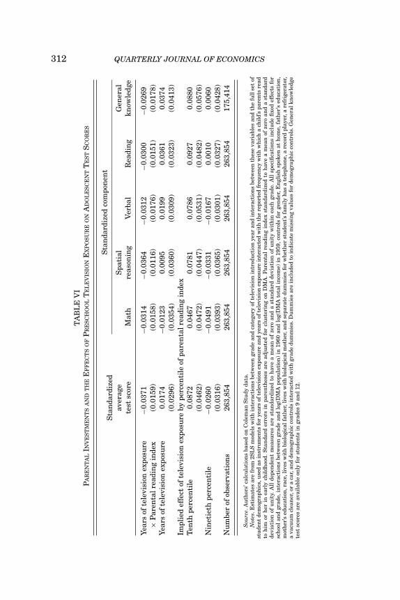
312 QUARTERLY JOURNAL OF ECONOMICS
TA
BL
EV
IP
AR
EN
TA
LIN
VE
ST
ME
NT
SA
ND
TH
EE
FF
EC
TS
OF
PR
ES
CH
OO
LT
EL
EV
ISIO
NE
XP
OS
UR
EO
NA
DO
LE
SC
EN
TT
ES
TS
CO
RE
S
Sta
nda
rdiz
edco
mpo
nen
tS
tan
dard
ized
aver
age
Spa
tial
Gen
eral
test
scor
eM
ath
reas
onin
gV
erba
lR
eadi
ng
know
ledg
e
Year
sof
tele
visi
onex
posu
re−0
.037
1−0
.031
4−0
.036
4−0
.031
2−0
.030
0−0
.026
9×
Par
enta
lrea
din
gin
dex
(0.0
159)
(0.0
158)
(0.0
116)
(0.0
176)
(0.0
151)
(0.0
178)
Year
sof
tele
visi
onex
posu
re0.
0174
−0.0
123
0.00
950.
0199
0.03
610.
0374
(0.0
296)
(0.0
354)
(0.0
360)
(0.0
309)
(0.0
323)
(0.0
413)
Impl
ied
effe
ctof
tele
visi
onex
posu
reby
perc
enti
leof
pare
nta
lrea
din
gin
dex
Ten
thpe
rcen
tile
0.08
720.
0467
0.07
810.
0786
0.09
270.
0880
(0.0
462)
(0.0
472)
(0.0
447)
(0.0
531)
(0.0
482)
(0.0
576)
Nin
etie
thpe
rcen
tile
−0.0
260
−0.0
491
−0.0
331
−0.0
167
0.00
100.
0060
(0.0
316)
(0.0
393)
(0.0
365)
(0.0
301)
(0.0
327)
(0.0
428)
Nu
mbe
rof
obse
rvat
ion
s26
3,85
426
3,85
426
3,85
426
3,85
426
3,85
417
5,41
4
Sou
rce.
Au
thor
s’ca
lcu
lati
ons
base
don
Col
eman
Stu
dyda
ta.
Not
es.E
stim
ates
are
from
2SL
Sm
odel
sw
ith
inte
ract
ion
sbe
twee
ngr
ade
and
cate
gory
ofte
levi
sion
intr
odu
ctio
nye
aran
din
tera
ctio
ns
betw
een
thes
eva
riab
les
and
the
full
set
ofst
ude
nt
dem
ogra
phic
s,u
sed
asin
stru
men
tsfo
rye
ars
ofte
levi
sion
expo
sure
and
year
sof
tele
visi
onex
posu
rein
tera
cted
wit
hth
ere
port
edfr
equ
ency
wit
hw
hic
ha
chil
d’s
pare
nts
read
toh
imor
her
inea
rly
chil
dhoo
d.S
tan
dard
erro
rsin
pare
nth
eses
are
adju
sted
for
clu
ster
ing
onD
MA
.P
aren
tal
read
ing
inde
xst
anda
rdiz
edto
hav
ea
mea
nof
zero
and
ast
anda
rdde
viat
ion
ofu
nit
y.A
llde
pen
den
tm
easu
res
are
stan
dard
ized
toh
ave
am
ean
ofze
roan
da
stan
dard
devi
atio
nof
un
ity
wit
hin
each
grad
e.A
llsp
ecifi
cati
ons
incl
ude
fixe
def
fect
sfo
rsc
hoo
lan
dgr
ade,
inte
ract
ion
sbe
twee
ngr
ade
and
log(
DM
Apo
pula
tion
)in
1960
and
log(
DM
Ato
tal
inco
me)
in19
59,c
ontr
ols
for
gen
der,
En
glis
hsp
oken
ath
ome,
fath
er’s
edu
cati
on,
mot
her
’sed
uca
tion
,rac
e,li
ves
wit
hbi
olog
ical
fath
er,l
ives
wit
hbi
olog
ical
mot
her
,an
dse
para
tedu
mm
ies
for
wh
eth
erst
ude
nt’s
fam
ily
has
ate
leph
one,
are
cord
play
er,a
refr
iger
ator
,a
vacu
um
clea
ner
,or
aca
r,an
dde
mog
raph
icco
ntr
ols
inte
ract
edw
ith
grad
edu
mm
ies.
Du
mm
ies
are
incl
ude
dto
indi
cate
mis
sin
gva
lues
for
dem
ogra
phic
con
trol
s.G
ener
alkn
owle
dge
test
scor
esar
eav
aila
ble
only
for
stu
den
tsin
grad
es9
and
12.

TELEVISION AND TEST SCORES 313
demographic groups in either television penetration or preschoolviewing hours rather than differences in the effect of television perse. In Appendix II, we use a limited amount of data on penetra-tion and hours to get a rough estimate of the importance of theseconfounds. We find that children with lower parental investmentare slightly less likely to own televisions but also watch slightlymore, conditional on owning. The combined effect of these forcesis such that correcting for heterogeneity in penetration and view-ership leaves the results essentially unchanged. Although datalimitations make these results far from definitive, they suggestthat much of the heterogeneity we identify reflects real variationin the effect of television.
The fact that households in which the benefits of television arelargest are also those in which children watch the most is an in-teresting result in its own right. For a more structured test of thishypothesis, we have computed each student’s predicted numberof television viewing hours per day by regressing reported tele-vision viewing on our standard vector of demographics. Amongstudents whose predicted television viewing is above average fortheir grade, the estimated effect of television exposure is to raisetest scores by 0.05 standard deviations. Among those whose pre-dicted viewing is below average, the estimated effect is almost ex-actly 0. Although by no means conclusive, this pattern is broadlyconsistent with a model in which television viewing hours arechosen optimally in response to variation across households inthe cognitive benefits (or costs) of television exposure.
VII. CONCLUSIONS
In this paper we show that the introduction of television inthe 1940s and 1950s had, if anything, small positive effects on theachievement of students exposed to television as preschoolers. Ourfindings suggest that much of the recent correlational evidenceattributing negative developmental effects to childhood televisionviewing may require reevaluation.
As discussed in the introduction, there are important caveatsto these results. First, our data speak only to the effects of earlychildhood television on academic achievement in adolescence.They do not provide evidence on contemporaneous effects, nordo they provide direct evidence on the effects of television onolder children. Second, it is possible that the type and variety

314 QUARTERLY JOURNAL OF ECONOMICS
of television content has changed over time in a way that wouldalter its effects on cognitive development.
We note, however, that there is no obvious reason to presumethat changes over time in content would make television’s effectmore negative. Indeed, Johnson (2005) argues that television pro-grams today are more cognitively demanding than programs inearlier decades, and the most popular shows among the childrenof 2003 (The Simpsons, American Idol, Malcolm in the Middle)do not seem obviously more or less intellectually rich than thosemost popular among the children of 1953 (I Love Lucy, Super-man, The Red Buttons Variety Show).38 Finally, a large numberof well-known educational television programs have been intro-duced since our sample period, many of which have been linkedto improvements in early childhood development (Kaiser FamilyFoundation 2005).
APPENDIX I: CROSS-SECTIONAL CORRELATION BETWEEN TELEVISION
AND TEST SCORES
In this section, we consider what results we might have ob-tained had we followed the approach of most previous literatureon the effects of television: looking at the cross-sectional corre-lation between television viewership and test scores. The resultsare informative about the direction and magnitude of biases thatmay arise in studies that take this approach.
Table A.2 presents regressions of both average test scoresand self-reported hours of (contemporaneous) television viewingon demographics. The first half of the table shows coefficientson family background variables, such as race and education.In almost all of these cases, the effects of these demographiccharacteristics on television hours are statistically significantand in the opposite direction from their effects on average testscores. Therefore, we would expect any unobserved variation inthese characteristics to tend to bias an OLS regression of testscores on television viewing towards finding negative effects oftelevision. The second half of the table shows that measures ofdurables ownership—a proxy for family income or wealth—tendto have positive effects on both television viewing and test scores,
38. Data on 1953 viewing patterns are from a survey of elementary pupils’“favorite” programs reported in Television magazine, April 1955, p. 84. Data on2003 viewing patterns are from Nielsen audience data for children ages 2–11.

TELEVISION AND TEST SCORES 315
TABLE A.1SUMMARY STATISTICS BY GRADE
Grade 6 Grade 9 Grade 12
Years of television exposure 3.966 3.358 1.765(0.762) (1.210) (1.194)
Year of television introductionEarly (1948 or earlier) 39% 40% 38%Middle (1948–1951) 25% 22% 23%Late (1952 or later) 36% 38% 39%
Father’s education (1–5) 4.041 3.898 3.793(1.992) (1.846) (1.859)
Mother’s education (1–5) 3.986 3.820 3.785(1.762) (1.532) (1.529)
Male 51% 51% 49%English not spoken at home 18% 17% 15%White 59% 62% 67%Lives with biological father 74% 74% 76%Lives with biological mother 89% 90% 91%Family has
Telephone 75% 79% 85%Record player 81% 87% 89%Refrigerator 93% 97% 98%Vacuum 70% 73% 78%Car 83% 84% 88%
Number of observations 120,075 131,074 95,413
Source. Authors’ calculations based on Coleman Study data.Notes. Standard deviations in parentheses. Table displays the mean value of each variable excluding
observations for which the variable is missing. Percentages refer to the share of students with the givencharacteristics within each grade.
controlling for family background. This finding is not surprisingbecause these proxies for wealth are highly correlated withtelevision ownership and are probably also highly related to thequality of the television set available in the household. So anOLS regression of test scores on television viewing that did notcontrol carefully for family income might find that television hasa positive effect on student performance. This type of bias seemsespecially likely in contexts where television ownership is notuniversal or where quality of sets or programming is likely to behighly variable with income.
These estimates suggest that OLS regressions of test scoreson television viewership can easily be subject to upward or down-ward bias, depending on which household characteristics are mea-sured well and which are measured poorly by the econometrician.OLS regressions of average test scores on self-reported viewing

316 QUARTERLY JOURNAL OF ECONOMICS
TABLE A.2THE CORRELATES OF TELEVISION VIEWING INTENSITY
Number of hours of Standardized averagetelevision viewing test score
(1) (2)
Male 0.0415 −0.0589(0.0080) (0.0077)
English not spoken at home 0.0009 −0.2046(0.0104) (0.0088)
Father’s education (index) −0.0509 0.0622(0.0034) (0.0018)
Mother’s education (index) −0.0306 0.0551(0.0043) (0.0017)
White −0.1750 0.4400(0.0241) (0.0334)
Lives with biological father −0.0537 0.0862(0.0071) (0.0065)
Lives with biological mother 0.1029 0.1992(0.0107) (0.0068)
Family hasTelephone 0.1199 0.1215
(0.0147) (0.0090)Record player 0.1716 0.0246
(0.0083) (0.0050)Refrigerator 0.3482 0.4555
(0.0320) (0.0161)Vacuum −0.0085 0.0696
(0.0114) (0.0104)Car 0.0446 0.0677
(0.0137) (0.0105)F (12, 135) 236.09 705.63(p-value) (<.0001) (<.0001)Number of observations 335,981 346,562Number of schools 800 800Number of DMAs 136 136
Source. Authors’ calculations based on Coleman Study data.Notes. Standard errors in parentheses are adjusted for clustering on DMA. Average test score is standard-
ized to have a mean of zero and a standard deviation of unity within each grade. All regressions include fixedeffects for school and grade and interactions between grade and log(DMA population) in 1960 and log(DMAtotal income) in 1959. Dummies are included to indicate missing values for demographic controls.
hours confirm this expectation. When we control for family back-ground measures such as race and education, but not for ourwealth proxies, we find an average effect of television viewing thatis positive and highly statistically significant. In contrast, whenwe include wealth proxies but not family background controls, theestimated effect becomes negative and statistically significant.
TELEVISION AND TEST SCORES 317
This finding may help to explain why correlational studies ofthe effects of television reach highly variable conclusions (Stras-burger 1986). Because these studies are only as good as the con-trols they employ, and because we find that omitted variablesproblems could lead either to an upward or downward bias of theeffects of television, it is not surprising that different academicstudies employing different econometric specifications reach rad-ically different conclusions. In a study that controls carefully forfamily background but not for income, we would expect to findpositive effects of television. By contrast, controlling carefully forincome or wealth but not for parental education and other back-ground characteristics will lead to a downward bias and findings ofdeleterious effects of television. We note, however, that we wouldexpect (and preliminary data analysis confirms) that the correla-tion between household wealth and television viewing hours tendsto be negative in more recent data, suggesting an unambiguousdownward bias in correlational estimates of the effect of televisionviewing on test scores.
APPENDIX II: SEPARATING HETEROGENEITY IN THE DIFFUSION,VIEWERSHIP, AND EFFECT OF TELEVISION
The first portion of Table A.3 repeats the estimates in columns(1) and (2) of Table V, which indicate that students whose mothersdid not have a high school degree benefited more from televisionthan students whose mothers had a high school degree. Thesedifferences may be confounded by the fact that parental educationis correlated with both the likelihood of television ownership andchildren’s viewing time. In this section, we show that simple cor-rections for these confounds have small effects on our substantiveconclusions. Indeed, because children with more educated parentswere more likely to live in a house with a television set but tendedto watch less conditional on ownership, biases from differencesin ownership and viewing intensity tend to pull in oppositedirections, and therefore to partially cancel one another out.
In the second portion of Table A.3 we adjust our estimates fordifferences in rates of television penetration across households.We compute average television penetration from 1949 to 1955 forboth high-school-educated and non-high-school-educated Galluppoll respondents (Roper Center for Public Opinion Research

318 QUARTERLY JOURNAL OF ECONOMICST
AB
LE
A.3
HE
TE
RO
GE
NE
ITY
INT
EL
EV
ISIO
NE
FF
EC
TS
AD
JUS
TE
DF
OR
PE
NE
TR
AT
ION
AN
DH
OU
RS
Sta
nda
rdiz
edco
mpo
nen
tS
tan
dard
ized
aver
age
Spa
tial
Gen
eral
test
scor
eM
ath
reas
onin
gV
erba
lR
eadi
ng
know
ledg
e
Un
adju
sted
esti
mat
esD
oes
mot
her
hav
eh
igh
sch
oold
egre
e?Ye
s0.
0135
−0.0
477
0.01
250.
0308
0.04
500.
0074
(0.0
297)
(0.0
422)
(0.0
395)
(0.0
294)
(0.0
316)
(0.0
529)
No
0.04
180.
0289
−0.0
342
0.04
820.
0942
0.06
57(0
.033
4)(0
.035
4)(0
.044
6)(0
.039
8)(0
.045
4)(0
.048
7)A
dju
sted
for
diff
eren
ces
inav
erag
ete
levi
sion
pen
etra
tion
,194
9–19
55D
oes
mot
her
hav
eh
igh
sch
oold
egre
e?Ye
s0.
0117
−0.0
414
0.01
090.
0267
0.03
900.
0064
(Sh
are
wit
hT
V=
0.43
)(0
.025
7)(0
.036
6)(0
.034
2)(0
.025
5)(0
.027
4)(0
.045
9)N
o0.
0474
0.03
28−0
.038
70.
0546
0.10
680.
0744
(Sh
are
wit
hT
V=
0.33
)(0
.037
8)(0
.040
1)(0
.050
5)(0
.045
1)(0
.051
4)(0
.055
1)A
dju
sted
for
diff
eren
ces
inav
erag
eda
ily
pres
choo
lvie
win
gh
ours
and
tele
visi
onpe
net
rati
onD
oes
mot
her
hav
eh
igh
sch
oold
egre
e?Ye
s0.
0122
−0.0
432
0.01
140.
0279
0.04
080.
0067
(Ave
rage
hou
rs=
1.32
)(0
.026
9)(0
.038
2)(0
.035
8)(0
.026
7)(0
.028
6)(0
.047
9)N
o0.
0461
0.03
19−0
.037
60.
0531
0.10
380.
0724
(Ave
rage
hou
rs=
1.42
)(0
.036
8)(0
.039
0)(0
.049
1)(0
.043
9)(0
.050
0)(0
.053
6)
Sou
rce.
Au
thor
s’ca
lcu
lati
ons
base
don
Col
eman
Stu
dyda
ta.
Not
es.E
stim
ates
are
from
2SL
Sm
odel
sw
ith
sam
ples
spli
tby
mot
her
’sed
uca
tion
.Sta
nda
rder
rors
inpa
ren
thes
esar
ead
just
edfo
rcl
ust
erin
gon
DM
A.A
llde
pen
den
tm
easu
res
are
stan
dard
ized
toh
ave
am
ean
ofze
roan
da
stan
dard
devi
atio
nof
un
ity
wit
hin
each
grad
e.A
llsp
ecifi
cati
ons
incl
ude
fixe
def
fect
sfo
rsc
hoo
lan
dgr
ade,
inte
ract
ion
sbe
twee
ngr
ade
and
log(
DM
Apo
pula
tion
)in
1960
and
log(
DM
Ato
tal
inco
me)
in19
59,
con
trol
sfo
rge
nde
r,E
ngl
ish
spok
enat
hom
e,fa
ther
’sed
uca
tion
,ra
ce,
live
sw
ith
biol
ogic
alfa
ther
,li
ves
wit
hbi
olog
ical
mot
her
,an
dse
para
tedu
mm
ies
for
wh
eth
erst
ude
nt’s
fam
ily
has
ate
leph
one,
are
cord
play
er,a
refr
iger
ator
,ava
cuu
mcl
ean
er,o
ra
car,
and
dem
ogra
phic
con
trol
sin
tera
cted
wit
hgr
ade
dum
mie
s.D
um
mie
sar
ein
clu
ded
toin
dica
tem
issi
ng
valu
esfo
rde
mog
raph
icco
ntr
ols.
Gen
eral
know
ledg
ete
stsc
ores
are
only
avai
labl
efo
rst
ude
nts
ingr
ades
9an
d12
.

TELEVISION AND TEST SCORES 319
1949–1955).39 Using these averages, we then compute the ratio ofeach group’s penetration to overall television penetration duringthis period and scale each coefficient accordingly. Since high-school-educated respondents to the Gallup poll tended to be about15% more likely to own televisions than the average respondentduring this period, we divide the coefficient (and standard error)on television exposure by 1.15 for students whose mothers havehigh school degrees. Similarly, since Gallup respondents who didnot complete high school were about 12% less likely to own atelevision than the average respondent, we divide the figures forstudents whose mothers did not complete high school by 0.88.As the second portion of Table A.3 shows, taking these adjust-ments into account makes little difference for our qualitativeconclusions.
In the third portion of Table A.3, we further adjust our es-timates to allow for differences in viewing intensity by parentaleducation. We estimate preschool viewing hours for each respon-dent in the Coleman sample by scaling reported hours of current(1965) daily viewership to reflect the difference in viewing inten-sity between preschoolers and adolescents.40 We then rescale thecoefficients for the high- and low-education groups by the ratioof the group’s average daily preschool viewing hours to the over-all average. Again, this adjustment does not make a substantialdifference.
UNIVERSITY OF CHICAGO AND NBERUNIVERSITY OF CHICAGO AND NBER
REFERENCES
Altonji, Joseph G., Todd E. Elder, and Christopher R. Taber, “Selection on Observedand Unobserved Variables: Assessing the Effectiveness of Catholic Schools,”Journal of Political Economy, 113 (1) (2005), 151–184.
39. Another way to avoid bias from different penetration rates would be toask whether television’s effect differs in counties with either high or low averageeducation levels. The fact that lower education counties might also have less pen-etration is already corrected for in the estimates because our exposure measureis built from county-level penetration data. We do not report these results here,but they show a similar pattern: in counties with lower-than-median rates of high-school completion, we estimate larger positive television effects on reading, verbal,and general knowledge scores than in counties with above-median education. Theeffect on reading scores in low-education counties is statistically significant at the5% level.
40. We scale each student’s reported hours of television viewing proportionallyso that the average predicted preschool viewing in each grade is equal to Schramm,Lyle, and Parker’s (1961) estimates of preschool viewing intensity in the 1950s.

320 QUARTERLY JOURNAL OF ECONOMICS
Alvermann, Donna E., Lynn C. Smith, and John E. Readence, “Prior KnowledgeActivation and the Comprehension of Compatible and Incompatible Text,”Reading Research Quarterly, 20 (4) (1985), 420–436.
American Academy of Pediatrics, “American Academy of Pediatrics: Children, Ado-lescents, and Television,” Pediatrics, 107 (2) (2001), 423–426.
Angrist, Joshua D. “Treatment Effect Heterogeneity in Theory and Practice,”Economic Journal, 114 (494) (2004), 83.
Barnett, W. Steven, “Long-Term Effects of Early Childhood Programs on Cognitiveand School Outcomes,” The Future of Children, 5 (3) (1995), 25–50.
Barnouw, Erik, Tube of Plenty: The Evolution of American Television. 2nd rev. ed.(New York: Oxford University Press, 1990).
Baum, Christopher F., Mark E. Schaffer, and Steven Stillman, “Instrumental Vari-ables and GMM: Estimation and Testing,” Stata Journal, 3 (1) (2003), 1–31.
Becker, Gary S. “A Theory of the Allocation of Time,” Economic Journal, 75 (299)(1965), 493–517.
Beentjes, Johannes W. J., and Tom H. A. Van der Voort, “Television’s Impact onChildren’s Reading Skills: A Review of Research,” Reading Research Quar-terly, 23 (4) (1988), 389–413.
Bertrand, Marianne, Esther Duflo, and Sendhil Mullainathan, “How Much ShouldWe Trust Differences-in-Differences Estimates?” Quarterly Journal of Eco-nomics, 119 (1) (2004), 249.
Bishop, John H. “Is the Test Score Decline Responsible for the Productivity GrowthDecline?” American Economic Review, 79 (1) (1989), 178–197.
Campbell, Frances A., and Craig T. Ramey, “Cognitive and School Outcomes forHigh-Risk African-American Students at Middle Adolescence: Positive Effectsof Early Intervention,” American Educational Research Journal, 32 (4) (1995),743–772.
Card, David, and Alan B. Krueger, “Does School Quality Matter? Returns to Edu-cation and the Characteristics of Public Schools in the United States,” Journalof Political Economy, 100 (1) (1992), 1–40.
Cascio, Elizabeth U. “Schooling Attainment and the Introduction of Kindergartensinto Public Schools,” mimeo, University of California, Davis, April 2004.
Christakis, Dimitri A., Frederick J. Zimmerman, David L. DiGiuseppe, and Car-olyn A. McCarty, “Early Television Exposure and Subsequent AttentionalProblems in Children,” Pediatrics, 113 (4) (2004), 708–713.
Coleman, James Samuel, and United States Office of Education and NationalCenter for Educational Statistics, Equality of Educational Opportunity(Washington, DC: U.S. Department of Health Education and Welfare Office ofEducation, 1966).
Cook, Thomas D., Hilary Appleton, Ross F. Conner, Ann Shaffer, Gary Tamkin,and Stephen J. Weber, “Sesame Street” Revisited (New York: Russell SageFoundation, 1975).
Cunha, Flavio, James J. Heckman, Lance Lochner, and Dimitriy V. Masterov,“Interpreting the Evidence on Life Cycle Skill Formation,” E. Hanushek andF. Welch, eds., in Handbook of the Economics of Education, 1st ed., Handbooksin Economics, Vol. 1 (Amsterdam: North-Holland, 2006).
Currie, Janet, “Early Childhood Education Programs,” Journal of Economic Per-spectives, 15 (2) (2001), 213–238.
Dahl, Gordon, and Stefano DellaVigna, “Does Movie Violence Increase ViolentCrime?” mimeo, UC Berkeley, June 2006.
DellaVigna, Stefano, and Ethan Kaplan, “The Fox News Effect: Media Bias andVoting,” Quarterly Journal of Economics, 122 (3) (2007).
Diaz-Guerrero, Rogelio, Isabel Reyes-Lagunes, Donald B. Witzke, and Wayne H.Holtzman, “Plaza Sesamo in Mexico: An Evaluation,” Journal of Communica-tion, 26 (2) (1976), 145–154.
Djankov, Simeon, Caralee McLiesh, Tatiana Nenova, and Andrei Shleifer, “WhoOwns the Media?” Journal of Law and Economics, 46 (2) (2003), 341–381.
Ehrenberg, Ronald G., and Dominic J. Brewer, “Did Teachers’ Verbal Ability andRace Matter in the 1960s? Coleman Revisited,” Economics of Education Re-view, 14 (1) (1995), 1.
Eisenberg, Azriel Louis, Children and Radio Programs: A Study of More than ThreeThousand Children in the New York Metropolitan Area (New York: ColumbiaUniversity Press, 1936).

TELEVISION AND TEST SCORES 321
Fox Meadow School PTA, “Radio for Children—Parents Listen In,” Child StudyMagazine, 11 (7) (1933).
Gaddy, Gary D., “Television’s Impact on High School Achievement,” Public OpinionQuarterly, 50 (3) (1986), 340–359.
Gentile, D. A., C. Oberg, N. E. Sherwood, M. Story, D. A. Walsh, and M. Hogan,“Well-Child Visits in the Video Age: Pediatricians and the American Academyof Pediatrics’ Guidelines for Children’s Media Use,” Pediatrics, 114 (5) (2004),1235–1241.
Gentzkow, Matthew, “Television and Voter Turnout,” Quarterly Journal of Eco-nomics, 121 (3) (2006), 931–972.
Gentzkow, Matthew, and Jesse M. Shapiro, “Media Bias and Reputation,” Journalof Political Economy, 114 (2) (2006), 280–316.
—— “Media, Education, and Anti-Americanism in the Muslim World,” Journal ofEconomic Perspectives, 18 (3) (2004), 117–133.
Glenn, Norval D., “Television Watching, Newspaper Reading, and Cohort Differ-ences in Verbal Ability,” Sociology of Education, 67 (3) (1994), 216–230.
Griliches, Zvi, “Hybrid Corn: An Exploration in the Economics of TechnologicalChange,” Econometrica, Journal of the Econometric Society, 25 (4) (1957),501–522.
Griliches, Zvi, and William M. Mason, “Education, Income, and Ability,” Journalof Political Economy, 80 (3) (1972), S74–S103.
Hancox, Robert J., Barry J. Milne, and Richie Poulton, “Association of TelevisionViewing during Childhood with Poor Educational Achievement,” Archive ofPediatrics & Adolescent Medicine, 159 (7) (2005), 614–618.
Hansen, Lars Peter, “Large Sample Properties of Generalized Method of MomentsEstimators,” Econometrica, 50 (4) (1982), 1029–1054.
Hanushek, Eric A., and John F. Kain, “On the Value of Equality of EducationalOpportunity as a Guide to Public Policy,” in On Equality of Educational Oppor-tunity, Frederick Mosteller and Daniel P. Moynihan, eds. (New York: RandomHouse, 1972).
Harrison, Linda Faye, and Tannis MacBeth Williams, “Television and CognitiveDevelopment,” in The Impact of Television: A Natural Experiment in ThreeCommunities, Tannis MacBeth Williams, ed. (London: Academic Press, 1986).
Hart, Betty, and Todd R. Risley, Meaningful Differences in the Everyday Experienceof Young American Children (Baltimore, MD: Paul H. Brookes Publishing Co.,1995).
—— The Social World of Children Learning to Talk (Baltimore, MD: Paul H.Brookes Publishing Co., 1999).
Heckman, James J., “Randomization as an Instrumental Variable,” Review of Eco-nomics and Statistics, 78 (2) (1996), 336–341.
Heckman, James J., and Yona, Rubinstein, “The Importance of Noncognitive Skills:Lessons from the GED Testing Program,” American Economic Review, 91 (2)(2001), 145–149.
Heckman, James J., and Guilherme Sedlacek, “Heterogeneity, Aggregation, andMarket Wage Functions: An Empirical Model of Self-Selection into the LaborMarket,” Journal of Political Economy, 93 (6) (1985), 1077–1125.
Hennigan, Karen M., Linda Heath, J. D. Wharton, M. L. Delrosario, T. D. Cook,and B. J. Calder, “Impact of the Introduction of Television on Crime in theUnited States: Empirical-Findings and Theoretical Implications,” Journal ofPersonality and Social Psychology, 42 (3) (1982), 461–477.
Hoxby, Caroline M., and M. Daniele Paserman, “Overidentification Tests withGrouped Data,” NBER Technical Working Paper 223 (February 1998).
Jencks, Christopher S., “The Quality of the Data Collected by the Equality ofEducational Opportunity Survey,” in On Equality of Educational Opportunity:Papers Deriving from the Harvard University Faculty Seminar on the ColemanReport, Frederick Mosteller and Daniel P. Moynihan, eds. (New York: VintageBooks, 1972).
Johnson, Steven, Everything Bad Is Good for You: How Today’s Popular Culture IsActually Making Us Smarter (New York: Riverhead Hardcover, 2005).
Kaiser Family Foundation, “The Effects of Electronic Media on Children Ages Zeroto Six: A History of Research,” 2005.

322 QUARTERLY JOURNAL OF ECONOMICS
Langer, Judith A., “Examining Background Knowledge and Text Comprehension,”Reading Research Quarterly, 19 (4) (1984), 468–481.
Maccoby, Eleanor E., “Television: Its Impact on School Children,” Public OpinionQuarterly, 15 (3) (1951), 421–444.
Moulton, Brent R., “An Illustration of a Pitfall in Estimating the Effects of Ag-gregate Variables on Micro Unit,” Review of Economics and Statistics, 72 (2)(1990), 334.
Olken, Benjamin A., “Do Television and Radio Destroy Social Capital? Evidencefrom Indonesian Villages,” NBER Working Paper No. 12561, October, 2006.
Parker, Edwin B., “The Effects of Television on Public Library Circulation,” PublicOpinion Quarterly, 27 (4) (1963), 578–589.
Pinon, Marites F., Aletha C. Huston, and John C. Wright, “Family Ecology andChild Characteristics that Predict Young Children’s Educational TelevisionViewing,” Child Development, 60 (4) (1989), 846–856.
Rice, Mabel L., “The Role of Television in Language Acquisition,” DevelopmentalReview, 3 (1983), 221–224.
Rice, Mabel L., and Linda Woodsmall, “Lessons from Television: Children’s WordLearning When Viewing,” Child Development, 59 (2) (1988), 420–429.
Rideout, Victoria J., Elizabeth A. Vandewater, and Ellen A. Wartella, “Zero to Six:Electronic Media in the Lives of Infants, Toddlers, and Preschoolers,” Tech.rept., Kailer Family Foundation, 2003.
Roper Center for Public Opinion Research, Gallup Polls, Vols. USAIPO1949-0441,USAIPO1950-0460, USAIPO1951-0470, USAIPO1953-0513, USAIPO1953-0514, USAIPO1953-0522, USAIPO1954-0529, USAIPO1954-0537,USAIPO1955-0546, USAIPO1955-0549 (Mansfield, CT: Gallup Organization,1949–1955).
Roslow, Sydney, “Programming Trends,” Television, 9 (4) (1952), 22–23.Rossiter, John R., and Thomas S. Robertson, “Children’s Television Viewing: An
Examination of Parent-Child Consensus,” Sociometry, 38 (3) (1975), 308–326.Roy, A. D. “Some Thoughts on the Distribution of Earnings,” Oxford Economic
Papers, 3 (2) (1951), 135–146.Ruggles, Steven, Matthew Sobek, Trent Alexander, Catherine A. Fitch, Ronald
Goeken, Patricia Kelly Hall, Miriam King, and Chad Ronnander, IntegratedPublic Use Microdata Series: Version 3.0 (www.ipums.org, 2004).
Schramm, Wilbur, Jack Lyle, and Edwin B. Parker, Television in the Lives of OurChildren (Stanford, CA: Stanford University Press, 1961).
Schweinhart, Lawrence J., Jeanne Montie, Zongping Xiang, W. Steven Barnett,Clive R. Belfield, and Milagros Nores, Lifetime Effects: The High/Scope PerryPreschool Study Through Age 40, Monographs of the High/Scope EducationalResearch Foundation (Ypsilanti, MI: High/Scope Press, 2005).
Slotten, Hugh Richard, Radio and Television Regulation: Broadcast Technologyin the United States, 1920–1960 (Baltimore: Johns Hopkins University Press,2000).
Sterling, Christopher H., and John M. Kittross, Stay Tuned: A History of AmericanBroadcasting, 3rd ed., LEA’s Communication Series (Mahwah, NJ: LawrenceErlbaum Associates, 2001).
Stock, James H., and Motohiro Yogo, “Testing for Weak Instruments in Linear IVRegression,” NBER Technical Working Paper 284, 2002.
Strasburger, V. C., “Does Television Affect Learning and School Performance?”Pediatrician, 13 (2-3) (1986), 141–7.
Stromberg, David, “Radio’s Impact on Public Spending,” Quarterly Journal of Eco-nomics, 119 (1) (2004), 189–221.
Television Bureau of Advertising, TV Basics 2003: A Report on the Growth andScope of Television (http://www.tvb.org/rcentral/mediattrendstracks/tvbasics,October 19, 2003).
Television Digest, Television Factbook (Washington, DC: Television Factbook, Inc.,various years).
Television Magazine, “Programming,” Television, 5 (1) (1948), 41–43.—— “Four Hundred Thousand Dollars a Week for the Children’s Market,” Televi-
sion, 8 (8) (1951), 21–22.—— “The Child Audience,” Television, 12 (4) (1955), 83–84.—— Market Book (New York: Frederick Kugel Company, various years).

TELEVISION AND TEST SCORES 323
Van Evra, Judith Page, Television and Child Development (Mahwah, NJ: LawrenceErlbaum Associates, 1998).
Winn, Marie, The Plug-In Drug: Television, Computers, and Family Life (New York:Penguin, 2002).
Wirtz, Willard, Harold Howe II, Bernard C. Watson, Ralph W. Tyler, Ledyard R.Tucker, Vivian H. T. Tom, Robert L. Thorndike, Barbara Thompson, ThomasW. F. Strand, Rosedith Sitgreaves, Wilbur Schramm, Katherine P. Layton,Owen B. Kiernan, H. Thomas James, Matina S. Horner, Edythe J. Gaines,Frank W. Erwin, Bruce K. Eckland, Luis C. Cortez, Sandra A. Clark, andBenjamin S. Bloom, On Further Examination: Report of the Advisory Panelon the Scholastic Aptitude Test Score Decline (New York: College EntranceExamination Board, 1977).
Zavodny, Madeline, “Does Watching Television Rot Your Mind? Evidence of theEffect on Test Scores,” Economics of Education Review, 25 (5) (2006), 565–573.
Zimmerman, Frederick J., and Dimitri A. Christakis, “Children’s Television View-ing and Cognitive Outcomes: A Longitudinal Analysis of National Data,”Archive of Pediatrics & Adolescent Medicine, 159 (7) (2005), 619–625.