arX

iv:1

712.

0125

0v2

[m

ath.

AG

] 1

3 Ju

n 20

18

The algebraic geometry of Kazhdan-Lusztig-Stanley polynomials

Nicholas Proudfoot

Department of Mathematics, University of Oregon, Eugene, OR 97403

njp@uoregon.edu

Abstract. Kazhdan-Lusztig-Stanley polynomials are a combinatorial generalization of Kazhdan-

Lusztig polynomials of Coxeter groups that include g-polynomials of polytopes and Kazhdan-

Lusztig polynomials of matroids. In the cases of Weyl groups, rational polytopes, and realizable

matroids, one can count points over finite fields on flag varieties, toric varieties, or reciprocal

planes to obtain cohomological interpretations of these polynomials. We survey these results

and unite them under a single geometric framework.

1 Introduction

The original definition of Kazhdan-Lusztig polynomials for a Coxeter group involves the relationship

between two bases for the Hecke algebra, however the polynomials are characterized by a purely

combinatorial recursion involving intervals in the Bruhat poset [KL79, Equation (2.2.a)]. Stanley

later generalized this recursive definition, replacing the Bruhat poset with an arbitrary locally

graded poset [Sta92, Definition 6.2(b)]. Stanley’s main motivation was the observation that the

g-polynomial of a polytope, which he introduced in [Sta87], arises very naturally in this way [Sta92,

Example 7.2]. Brenti went on to generalize this definition slightly further to weakly ranked posets,

and dubbed the corresponding polynomials Kazhdan-Lusztig-Stanley polynomials [Bre99].

More examples have been studied since then, including Kazhdan-Lusztig polynomials of matroids,

which were introduced in [EPW16] and have been the subject of much recent research.

In a sequel to their first paper, Kazhdan and Lusztig proved that their polynomials can be

interpreted as Poincare polynomials for the stalk cohomology groups of the intersection cohomology

sheaves of Schubert varieties [KL80, Theorem 4.3]. The idea of the proof is that the combinatorial

recursion for the polynomials is precisely the recursion for the Poincare polynomials that one obtains

by applying the Lefschetz fixed point formula to the Frobenius automorphism of certain subvarieties

of the flag variety. This technique has subsequently been imported to the study of other classes

of Kazhdan-Lusztig-Stanley polynomials, including Kazhdan-Lusztig polynomials of affine Weyl

groups [Lus83, Section 11], g-polynomials of rational polytopes [DL91, Theorem 6.2] and [Fie91,

Theorem 1.2], h-polynomials of broken circuit complexes of a rational hyperplane arrangements

[PW07, Theorem 4.3], and Kazhdan-Lusztig polynomials of hyperplane arrangements [EPW16,

Theorem 3.10].

While the various instances of the aforementioned Lefschetz argument are all based on the same

idea, they all involve a rather messy induction, and it can be difficult to determine exactly what

ingredients are needed to make the argument work. The purpose of this document is to do exactly

that. After reviewing the combinatorial theory of Kazhdan-Lusztig-Stanley polynomials (Section

1

2), we lay out a basic geometric framework for interpreting these polynomials as Poincare polyno-

mials of stalks of intersection cohomology sheaves on a stratified variety (Section 3). In particular,

we show that each of the aforementioned results can be obtained as an application of our general

machine (Section 4) without having to redo the inductive argument each time.

Though our main purpose is to survey and unify various old results, there is one new concept

that we introduce and study here. When defining Kazhdan-Lusztig-Stanley polynomials, there is

a left versus right convention that appears in the definition. The left Kazhdan-Lusztig-Stanley

polynomials for a weakly graded poset P coincide with the right Kazhdan-Lusztig-Stanley poly-

nomials for the opposite poset P ∗ (Remark 2.4). In particular, since the Bruhat poset of a finite

Coxeter group is self-opposite and the face poset of a polytope is opposite to the face poset of

the dual polytope, the left/right issue (while at times confusing) is not so important. The same

statement is not true of the lattice of flats of a matroid, and indeed the right Kazhdan-Lusztig-

Stanley polynomials of a matroid are interesting while the left ones are trivial (Example 2.13). We

introduce a class of polynomials called Z-polynomials (Section 2.3) that depend on both the left

and right Kazhdan-Lusztig-Stanley polynomials. In the case of the lattice of flats of a matroid,

these polynomials coincide with the polynomials introduced in [PXY18].

Under certain assumptions, we use another Lefschetz argument to interpret our Z-polynomials a

Poincare polynomials for the global intersection cohomology of the closure of a stratum in our strat-

ified variety. In particular, in the case of the Bruhat poset of a Weyl group, the Z-polynomials are

intersection cohomology Poincare polynomials of Richardson varieties (Theorem 4.3); in the case of

the lattice of flats of a hyperplane arrangements, they are intersection cohomology Poincare polyno-

mials of arrangement Schubert varieties (Theorem 4.17); and in the case of the affine Grassmannian,

they are intersection cohomology Poincare polynomials of closures of Schubert cells (Corollary 4.8).

It would be interesting to know whether the Z-polynomial of a rational polytope has a cohomo-

logical interpretation in terms of toric varieties. These polynomials are closely related to a family

of polynomials defined by Batyrev and Borisov (Remark 2.15), but they are not quite the same.

1.1 Things that this paper is not about

There are many interesting questions about Kazhdan-Lusztig-Stanley polynomials that we will

mention briefly here but not address in the main part of the paper.

• By giving a cohomological interpretation of a Kazhdan-Lusztig-Stanley polynomial, one can in-

fer that it has non-negative coefficients. There is a rich history of pursuing the non-negativity

of certain classes Kazhdan-Lusztig polynomials in the absence of a geometric interpretation.

This was achieved by Elias and Williamson for Kazhdan-Lusztig polynomials of Coxeter

groups that are not Weyl groups [EW14, Conjecture 1.2(1)] and by Karu for polytopes that

are not rational [Kar04, Theorem 0.1] (see also [Bra06, Theorem 2.4(b)]). Braden, Huh, Math-

erne, Wang, and the author are working to prove an analogous theorem for matroids that are

not realizable by hyperplane arrangements.

2

• For many specific classes of Kazhdan-Lusztig-Stanley polynomials, it is interesting to ask

what polynomials can arise. Polo proved that any polynomial with non-negative coefficients

and constant term 1 is equal to a Kazhdan-Lusztig polynomial for a symmetric group [Pol99].

In contrast, the g-polynomial of a polytope cannot have internal zeros [Bra06, Theorem 1.4].

If the polytope is simplicial, then the sequence of coefficients is an M-sequence [Sta80], and

this is conjecturally the case for all polytopes; see [Bra06, Section 1.2] for a discussion of

this conjecture. Kazhdan-Lusztig polynomials of matroids are conjectured to always be log

concave with no internal zeros [EPW16, Conjecture 2.5] and even real-rooted [GPY17, Con-

jecture 3.2], and a similar conjecture has been made for Z-polynomials of matroids [PXY18,

Conjecture 5.1].

• Classical Kazhdan-Lusztig polynomials were originally defined in terms of the Kazhdan-

Lusztig basis for the Hecke algebra. More generally, Du defines the notion of an IC basis for

a free Z[t, t−1]-module equipped with an involution [Du94], and Brenti proves that this notion

is essentially equivalent to the theory of Kazhdan-Lusztig-Stanley polynomials [Bre03, Theo-

rem 3.2]. Multiplication in the Hecke algebra is compatible with the involution, which Brenti

shows is a very special property [Bre03, Theorem 4.1]. Furthermore, the structure constants

for multiplication in the Kazhdan-Lusztig basis of the Hecke algebra are positive [EW14,

Conjecture 1.2(2)], and Du asks whether this holds in some greater generality [Du94, Section

5]. In the case of Kazhdan-Lusztig polynomials of matroids, a candidate algebra structure

was described and positivity was conjectured [EPW16, Conjecture 4.2], but that conjecture

turned out to be false (see Section 4.6 of the arXiv version). It is unclear whether this conjec-

ture could be salvaged by changing the definition of the algebra structure, or more generally

when a particular collection of Kazhdan-Lusztig-Stanley polynomials comes equipped with a

nice algebra structure on its associated module.

Acknowledgments: This work was greatly influenced by conversations with many people, including

Sara Billey, Tom Braden, Ben Elias, Jacob Matherne, Victor Ostrik, Richard Stanley, Minh-Tam

Trinh, Max Wakefield, Ben Webster, Alex Yong, and Ben Young. The author is also grateful to

the referee for many helpful comments. The author is supported by NSF grant DMS-1565036.

2 Combinatorics

We begin by reviewing the combinatorial theory of Kazhdan-Lusztig-Stanley polynomials, which

was introduced in [Sta92, Section 6] and further developed in [Dye93, Bre99, Bre03]. We also

introduce Z-polynomials (Section 2.3) and study their basic properties.

3

2.1 The incidence algebra

Let P be a poset. We say that P is locally finite if, for all x ≤ z ∈ P , the set

[x, z] := {y ∈ P | x ≤ y ≤ z}

is finite. Let

I(P ) :=∏

x≤y

Z[t].

For any f ∈ I(P ) and x < y ∈ P , let fxy(t) ∈ Z[t] denote the corresponding component of f . If P

is locally finite, then I(P ) admits a ring structure with product given by convolution:

(fg)xz(t) :=∑

x≤y≤z

fxy(t)gyz(t).

The identity element is the function δ ∈ I(P ) with the property that δxy = 1 if x = y and 0

otherwise.

Let r ∈ I(P ) be a function satisfying the following conditions:

• rxy ∈ Z ⊂ Z[t] for all x ≤ y ∈ P (we will refer to rxy(t) simply as rxy)

• if x < y, then rxy > 0

• if x ≤ y ≤ z, then rxy + ryz = rxz.

Such a function is called a weak rank function [Bre99, Section 2]. We will use the terminology

weakly ranked poset to refer to a locally finite poset equipped with a weak rank function, and

we will suppress r from the notation when there is no possibility for confusion.

For any weakly ranked poset P , let I (P ) ⊂ I(P ) denote the subring of functions f with the

property that the degree of fxy(t) is less than or equal to rxy for all x ≤ y. The ring I (P ) admits

an involution f 7→ f defined by the formula

fxy(t) := trxyfxy(t−1).

Lemma 2.1. An element f ∈ I(P ) has an inverse (left or right) if and only if fxx(t) = ±1 for all

x ∈ P . In this case, the left and right inverses are unique and they coincide. If f ∈ I (P ) ⊂ I(P )

is invertible, then f−1 ∈ I (P ).

Proof. An element g is a right inverse to f if and only if gxx(t) = fxx(t)−1 and

fxx(t)gxz(t) = −∑

x<y≤z

fxy(t)gyz(t)

for all x < z. The first equation has a solution if and only if fxx(t) = ±1, in which case the second

equation also has a unique solution. If f ∈ I (P ), it is clear that g ∈ I (P ), as well. The argument

for left inverses is identical, so it remains only to show that left and right inverses coincide.

4

Let g be right inverse to f . Then g is also left inverse to some function, which we will denote

h. We then have

f = fδ = f(gh) = (fg)h = δh = h,

so g is left inverse to f , as well.

2.2 Right and left KLS-functions

An element κ ∈ I (P ) is called a P -kernel if κxx(t) = 1 for all x ∈ P and κ−1 = κ. Let

I1/2(P ) :={

f ∈ I (P )∣

∣

∣fxx(t) = 1 for all x ∈ P and deg fxy(t) < rxy/2 for all x < y ∈ P

}

.

Various versions of the following theorem appear in [Sta92, Corollary 6.7], [Dye93, Proposition 1.2],

and [Bre99, Theorem 6.2].

Theorem 2.2. If κ ∈ I (P ) is a P-kernel, there exists a unique pair of functions f, g ∈ I1/2(P )

such that f = κf and g = gκ.

Proof. We will prove existence and uniqueness of f ; the proof for g is identical. Fix elements

x < w ∈ P , and suppose that fyw(t) has been defined for all x < y ≤ w. Let

Qxw(t) :=∑

x<y≤w

κxy(t)fyw(t) ∈ Z[t].

The equation f = κf for the interval [x,w] translates to

fxw(t)− fxw(t) = Qxw(t).

It is clear that there is at most one polynomial fxw(t) of degree strictly less than rxw/2 satisfying

this equation. The existence of such a polynomial is equivalent to the statement

trxwQxw(t−1) = −Qxw(t).

5

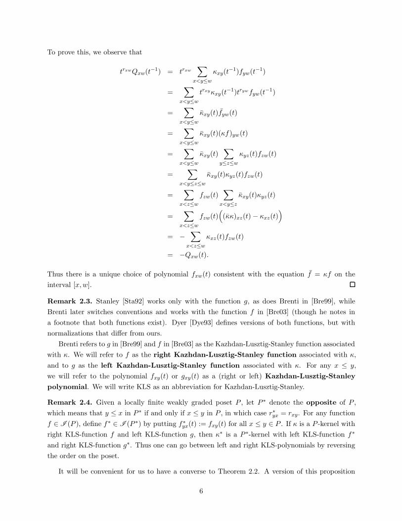
To prove this, we observe that

trxwQxw(t−1) = trxw

∑

x<y≤w

κxy(t−1)fyw(t

−1)

=∑

x<y≤w

trxyκxy(t−1)trywfyw(t

−1)

=∑

x<y≤w

κxy(t)fyw(t)

=∑

x<y≤w

κxy(t)(κf)yw(t)

=∑

x<y≤w

κxy(t)∑

y≤z≤w

κyz(t)fzw(t)

=∑

x<y≤z≤w

κxy(t)κyz(t)fzw(t)

=∑

x<z≤w

fzw(t)∑

x<y≤z

κxy(t)κyz(t)

=∑

x<z≤w

fzw(t)(

(κκ)xz(t)− κxz(t))

= −∑

x<z≤w

κxz(t)fzw(t)

= −Qxw(t).

Thus there is a unique choice of polynomial fxw(t) consistent with the equation f = κf on the

interval [x,w].

Remark 2.3. Stanley [Sta92] works only with the function g, as does Brenti in [Bre99], while

Brenti later switches conventions and works with the function f in [Bre03] (though he notes in

a footnote that both functions exist). Dyer [Dye93] defines versions of both functions, but with

normalizations that differ from ours.

Brenti refers to g in [Bre99] and f in [Bre03] as the Kazhdan-Lusztig-Stanley function associated

with κ. We will refer to f as the right Kazhdan-Lusztig-Stanley function associated with κ,

and to g as the left Kazhdan-Lusztig-Stanley function associated with κ. For any x ≤ y,

we will refer to the polynomial fxy(t) or gxy(t) as a (right or left) Kazhdan-Lusztig-Stanley

polynomial. We will write KLS as an abbreviation for Kazhdan-Lusztig-Stanley.

Remark 2.4. Given a locally finite weakly graded poset P , let P ∗ denote the opposite of P ,

which means that y ≤ x in P ∗ if and only if x ≤ y in P , in which case r∗yx = rxy. For any function

f ∈ I (P ), define f∗ ∈ I (P ∗) by putting f∗yx(t) := fxy(t) for all x ≤ y ∈ P . If κ is a P -kernel with

right KLS-function f and left KLS-function g, then κ∗ is a P ∗-kernel with left KLS-function f∗

and right KLS-function g∗. Thus one can go between left and right KLS-polynomials by reversing

the order on the poset.

It will be convenient for us to have a converse to Theorem 2.2. A version of this proposition

6

appears in [Sta92, Theorem 6.5].

Proposition 2.5. Suppose that f ∈ I1/2(P ). Then

1. f is invertible.

2. f f−1 is a P -kernel with f as its associated right KLS-function.

3. f−1f is a P -kernel with f as its associated left KLS-function.

Proof. By Lemma 2.1, f is invertible. We have (f f−1)−1 = f f−1 = ff−1, so ff−1 is a P -kernel.

Since f = f(f−1f) = (f f−1)f , the uniqueness part of Theorem 2.2 tells us that f is equal to the

associated right KLS-function. The last statement follows similarly.

2.3 The Z-function

We will call a function Z ∈ I (P ) symmetric if Z = Z. Let κ be a P -kernel with right KLS-

function f and left KLS-function g. Let Z := gκf ∈ I (P ); we will refer to Z as the Z-function

associated with κ, and to each Zxy(t) as a Z-polynomial.

Proposition 2.6. We have Z = gf = gf . In particular, Z is symmetric.

Proof. Since g = gκ, we have Z = gκf = gf . Since f = κf , we have Z = gκf = gf .

We have the following converse to Proposition 2.6.

Proposition 2.7. Suppose that f, g ∈ I1/2(P ). Then f and g are the right and left KLS-functions

for a single P -kernel κ if and only if gf is symmetric.

Proof. Let κf := f f−1 and κg := g−1g. By Proposition 2.5, f is the right KLS-function of κf and

g is the left KLS-function of κg. Then gf = gκgf and gf = gκff . Multiplying on the left by g−1

and on the right by f−1, we see that these two functions are the same if and only if κf = κg.

The following version of Proposition 2.7 will be useful in Section 3.4. It allows us to relax both

the symmetry assumption and the conclusion of Proposition 2.7.

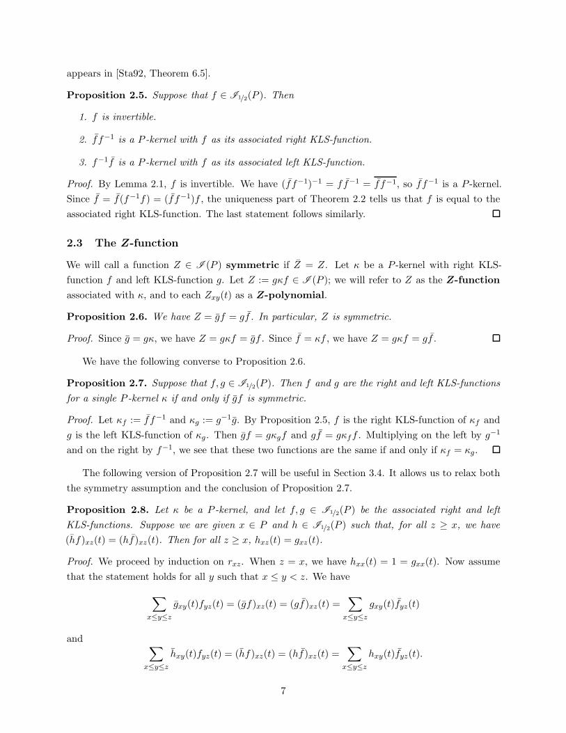
Proposition 2.8. Let κ be a P -kernel, and let f, g ∈ I1/2(P ) be the associated right and left

KLS-functions. Suppose we are given x ∈ P and h ∈ I1/2(P ) such that, for all z ≥ x, we have

(hf)xz(t) = (hf)xz(t). Then for all z ≥ x, hxz(t) = gxz(t).

Proof. We proceed by induction on rxz. When z = x, we have hxx(t) = 1 = gxx(t). Now assume

that the statement holds for all y such that x ≤ y < z. We have

∑

x≤y≤z

gxy(t)fyz(t) = (gf)xz(t) = (gf)xz(t) =∑

x≤y≤z

gxy(t)fyz(t)

and∑

x≤y≤z

hxy(t)fyz(t) = (hf)xz(t) = (hf)xz(t) =∑

x≤y≤z

hxy(t)fyz(t).

7

Subtracting these two equations and applying our inductive hypothesis, we have

gxz(t)− hxz(t) = trxz(

gxz(t)− hxz(t))

.

Since deg(gxz − hxz) < rxz/2, this implies that gxz(t) = hxz(t).

Proposition 2.9. Let κ ∈ I (P ) be a P -kernel, and let P ∗ be the opposite of P . Then Z∗ ∈ I (P ∗)

is the Z-polynomial associated with the P ∗-kernel κ∗.

Proof. By Remark 2.4, the left KLS-polynomial associated with κ∗ is f∗, and the right KLS-

polynomial is g∗. Thus the Z-polynomial is f∗κ∗g∗ = (gκf)∗ = Z∗.

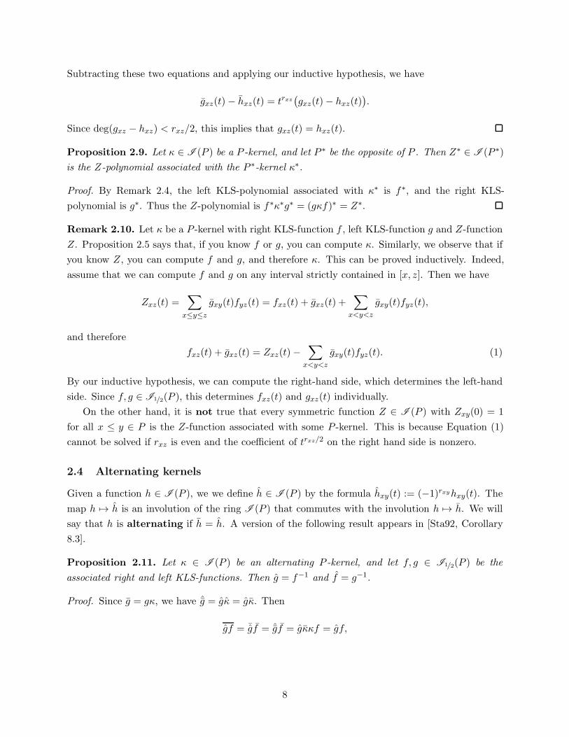
Remark 2.10. Let κ be a P -kernel with right KLS-function f , left KLS-function g and Z-function

Z. Proposition 2.5 says that, if you know f or g, you can compute κ. Similarly, we observe that if

you know Z, you can compute f and g, and therefore κ. This can be proved inductively. Indeed,

assume that we can compute f and g on any interval strictly contained in [x, z]. Then we have

Zxz(t) =∑

x≤y≤z

gxy(t)fyz(t) = fxz(t) + gxz(t) +∑

x<y<z

gxy(t)fyz(t),

and therefore

fxz(t) + gxz(t) = Zxz(t)−∑

x<y<z

gxy(t)fyz(t). (1)

By our inductive hypothesis, we can compute the right-hand side, which determines the left-hand

side. Since f, g ∈ I1/2(P ), this determines fxz(t) and gxz(t) individually.

On the other hand, it is not true that every symmetric function Z ∈ I (P ) with Zxy(0) = 1

for all x ≤ y ∈ P is the Z-function associated with some P -kernel. This is because Equation (1)

cannot be solved if rxz is even and the coefficient of trxz/2 on the right hand side is nonzero.

2.4 Alternating kernels

Given a function h ∈ I (P ), we we define h ∈ I (P ) by the formula hxy(t) := (−1)rxyhxy(t). The

map h 7→ h is an involution of the ring I (P ) that commutes with the involution h 7→ h. We will

say that h is alternating if h = h. A version of the following result appears in [Sta92, Corollary

8.3].

Proposition 2.11. Let κ ∈ I (P ) be an alternating P -kernel, and let f, g ∈ I1/2(P ) be the

associated right and left KLS-functions. Then g = f−1 and f = g−1.

Proof. Since g = gκ, we have ˆg = gκ = gκ. Then

gf = ¯gf = ˆgf = gκκf = gf,

8

thus gf is symmetric. However, since f, g ∈ I1/2(P ), we have deg(gf)xy(t) < rxy/2 for all x < y,

so this implies that (gf)xy(t) = 0 for all x < y. On the other hand, (gf)xx(t) = gxx(t)fxx(t) = 1.

Thus gf = δ, and therefore g = f−1. The second statement follows immediately.

2.5 Examples

We now discuss a number of examples of P -kernels along their associated KLS-functions and Z-

functions. All of these examples will be revisited in Section 4.

Example 2.12. Let W be a Coxeter group, equipped with the Bruhat order and the rank function

given by the length of an element of W . The classical R-polynomials {Rvw(t) | v ≤ w ∈ W}

form a W -kernel, and the classical Kazhdan-Lusztig polynomials {fxy(t) | v ≤ w ∈ W} are the

associated right KLS-polynomials. These polynomials were introduced by Kazhdan and Lusztig

[KL79], and they were one of the main motivating examples in Stanley’s work [Sta92, Example

6.9].

If W is finite, then there is a maximal element w0 ∈ W , and left multiplication by w0 defines

an order-reversing bijection of W with the property that, if v ≤ w, then Rvw(t) = R(w0w)(w0v)(t)

[Lus03, Lemma 11.3]. It follows from Remark 2.4 that gvw(t) = f(w0w)(w0v)(t). In addition, R is

alternating [KL79, Lemma 2.1(i)], hence Proposition 2.11 tells us that g = f−1 and f = g−1.

Example 2.13. Let P be any locally finite weakly ranked poset. Define ζ ∈ I (P ) by the formula

ζxy(t) = 1 for all x ≤ y ∈ P . The element µ := ζ−1 ∈ I (P ) is called the Mobius function,

and the product χ := µζ = ζ−1ζ is called the characteristic function of P . We then have

χ−1 = ζ−1ζ = χ, so χ is a P -kernel. Proposition 2.5(3) tells us that the associated left KLS-

function is ζ; this was observed by Stanley in [Sta92, Example 6.8]. However, the associated right

KLS-function f can be much more interesting! (In particular, χ is generally not alternating.) For

example, if P is the lattice of flats of a matroid M with the usual weak rank function, with minimum

element 0 and maximum element 1, then f01(t) is the Kazhdan-Lusztig polynomial of M as

defined in [EPW16], and Z01(t) is the Z-polynomial of M as defined in [PXY18]. In general, the

coefficients of fxy(t) can be expressed as alternating sums of multi-indexed Whitney numbers for

the interval [x, y] ⊂ P ; see [Bre99, Corollary 6.5], [Wak18, Theorem 5.1], and [PXY18, Theorem

3.3] for three different formulations of this result.

Example 2.14. Let P be any locally finite weakly ranked poset. Define λ ∈ I (P ) by the formula

λxy(t) = (t − 1)rxy for all x ≤ y ∈ P . The weakly ranked poset P is called locally Eulerian

if µxy(t) = (−1)rxy for all x ≤ y ∈ P , which is equivalent to the condition that λ is a P -kernel

[Sta92, Proposition 7.1]. The poset of faces of a polytope, with weak rank function given by relative

dimension (where dim ∅ = −1), is Eulerian. More generally, any fan is an Eulerian poset.

Let ∆ be a polytope, let P be the poset of faces of ∆, and let f and g be the associated right

and left KLS-functions. Then g∅∆(t) is called the g-polynomial of ∆ [Sta92, Example 7.2]. Since

the dual polytope ∆∗ has the property that its face poset is opposite to P , and since λ depends

only on the weak rank function, Remark 2.4 tells us that the right KLS-polynomial f∅∆(t) is equal

9

to the g-polynomial of ∆∗. On the other hand, since λ is clearly alternating, Proposition 2.11 tells

us that g = f−1 and f = g−1 [Sta92, Corollary 8.3].

Remark 2.15. For P locally Eulerian, Batyrev and Borisov define an element B ∈∏

x≤y∈P Z[u, v]

[BB96, Definition 2.7]. Let B′ ∈ I (P ) be the function obtained from B by setting u = −t and

v = −1. The defining equation for B transforms into the equation B′ ¯f = f . Using the fact that

f = g−1, this means that B′ = f g. Thus B′ is similar to Z = gf , but it is not quite the same. In

particular, B′ need not be symmetric.

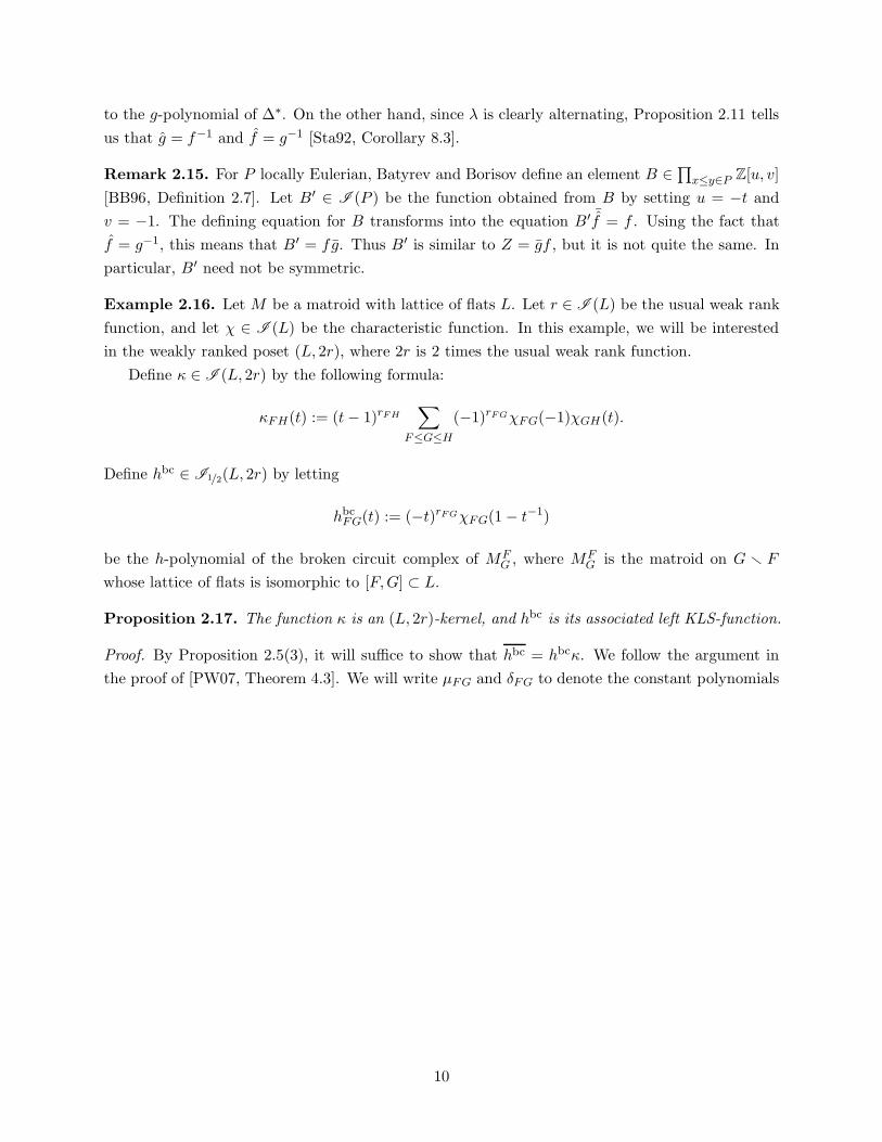
Example 2.16. Let M be a matroid with lattice of flats L. Let r ∈ I (L) be the usual weak rank

function, and let χ ∈ I (L) be the characteristic function. In this example, we will be interested

in the weakly ranked poset (L, 2r), where 2r is 2 times the usual weak rank function.

Define κ ∈ I (L, 2r) by the following formula:

κFH(t) := (t− 1)rFH

∑

F≤G≤H

(−1)rFGχFG(−1)χGH(t).

Define hbc ∈ I1/2(L, 2r) by letting

hbcFG(t) := (−t)rFGχFG(1− t−1)

be the h-polynomial of the broken circuit complex of MFG , where MF

G is the matroid on G r F

whose lattice of flats is isomorphic to [F,G] ⊂ L.

Proposition 2.17. The function κ is an (L, 2r)-kernel, and hbc is its associated left KLS-function.

Proof. By Proposition 2.5(3), it will suffice to show that hbc = hbcκ. We follow the argument in

the proof of [PW07, Theorem 4.3]. We will write µFG and δFG to denote the constant polynomials

10

µFG(t) and δFG(t). For all D ≤ J , we have

(hbcκ)DJ (t) =∑

D≤F≤J

hbcDF (t)κFJ(t)

=∑

D≤F≤H≤J

(t− 1)rFJ (−1)rFHχFH(−1)χHJ (t)(−t)rDFχDF (1− t−1)

=∑

D≤E≤F≤G≤H≤I≤J

(t− 1)rFJ (−1)rFHµFG(−1)rGHµHItrIJ (−t)rDFµDE(1− t−1)rEF

=∑

D≤E≤F≤G≤H≤I≤J

µDEµFGµHI(−1)rDGtrDE+rIJ (t− 1)rEJ

=∑

D≤E≤G≤I≤J

µDE(−1)rDGtrDE+rIJ (t− 1)rEJ

∑

E≤F≤G

µFG

∑

G≤H≤I

µHI

=∑

D≤E≤G≤I≤J

µDE(−1)rDGtrDE+rIJ (t− 1)rEJ δEGδGI

=∑

D≤E≤J

µDE(−1)rDE trDJ (t− 1)rEJ

= (−t)rDJ

∑

D≤E≤J

µDE(1− t)rEJ

= t2rDJ (−t−1)rDJχDJ(1− t)

= trDJhbcDJ(t−1)

= hbcDJ(t).

This completes the proof.

3 Geometry

In this section we give a general geometric framework for interpreting right KLS-polynomials in

terms of the stalks of intersection cohomology sheaves on a stratified space. Under some additional

assumptions, we also give cohomological interpretations for the associated Z-polynomials. Our

primary reference for technical properties of intersection cohomology will be the book of Kiehl and

Weissauer [KW01], however, a reader who is learning this material for the first time might also

benefit from the friendly discussion in the book of Kirwan and Woolf [KW06, Section 10.4].

3.1 The setup

Fix a finite field Fq, an algebraic closure Fq, and a prime ℓ that does not divide q. For any variety

Z over Fq, let ICZ denote the ℓ-adic intersection cohomology sheaf on the variety Z(Fq). We adopt

the convention of not shifting ICZ to make it perverse. In particular, if Z is smooth, then ICZ is

isomorphic to the constant sheaf in degree zero.

11

Suppose that we have a variety Y over Fq and a stratification

Y =⊔

x∈P

Vx.

By this we mean that each stratum Vx is a smooth connected subvariety of Y and the closure of each

stratum is itself a union of strata. We define a partial order on P by putting x ≤ y ⇐⇒ Vx ⊂ Vy,

and a weak rank function by the formula rxy = dimVy − dimVx. Fix a point ex ∈ Vx for each

x ∈ P .

Next, suppose that we have a stratification preserving Gm-action ρx : Gm → Aut(Y ) for each

x ∈ P and an affine Gm-subvariety Cx ⊂ Y with the following properties:

• Cx is a weighted affine cone with respect to ρx with cone point ex. In other words, the Z-

grading on the affine coordinate ring Fq[Cx] induced by ρx is non-negative and the vanishing

locus of the ideal of positively graded elements is {ex}.

• For all x, y ∈ P , let

Uxy := Cx ∩ Vy and Xxy := Cx ∩ Vy.

We require that the restriction of ICVyto Cx(Fq) is isomorphic to ICXxy .

Note that the variety Xxy is a closed Gm-equivariant subvariety of Cx, therefore it is either

empty or a weighted affine cone with cone point ex. We have

ex ∈ Xxy ⇐⇒ ex ∈ Vy ⇐⇒ x ≤ y,

so Xxy is nonempty if and only if x ≤ y.

Lemma 3.1. For all x ≤ z, we have Xxz =⊔

x≤y≤z

Uxy.

Proof. We have Xxz = Cx ∩ Vz = Cx ∩⊔

y≤z Vy =⊔

y≤z Uxy. If x is not less than or equal to Y ,

then Xxy is empty, thus so is Uxy.

The condition on restrictions of IC sheaves is somewhat daunting. In each of our families of

examples, we will check this condition by means of a group action, using the following lemma.

Lemma 3.2. Suppose that Y is equipped with an action of an algebraic group G preserving the

stratification. Suppose in addition that, for each x ∈ P , there exists a subgroup Gx ⊂ G such that

the composition

ϕx : Gx × Cx → G× Y → Y

is an open immersion. Then for all x ≤ y ∈ P , the restriction of ICVyto Cx(Fq) is isomorphic to

ICXxy .

12

Proof. Since ϕx is an open immersion, we have ϕ−1x ICVy

∼= ICϕ−1x (Vy)

as sheaves on Gx(Fq)×Cx(Fq)

for all x, y ∈ P . Since the action of G on Y preserves the stratification, we have

ϕ−1x (Vy) = Gx × (Cx ∩ Vy) = Gx ×Xxy,

so ϕ−1x ICVy

∼= ICGx ⊠ ICXxy . Since Gx is smooth, ICGx is the constant sheaf on Gx. Thus, if we

further restrict to Cx(Fq) ∼= {idGx} × Cx(Fq), we obtain ICXxy .

Remark 3.3. In some of our examples (Sections 4.2 and 4.3), the Gm-action ρx will not actually

depend on x. In other examples (Sections 4.1 and 4.4), it will depend on x.

3.2 Intersection cohomology

We will write IH∗(Z) and IH∗c(Z) to denote the ordinary and compactly supported cohomology of

ICZ . Given a point p ∈ Z, we will write IH∗p(Z) to denote the cohomology of the stalk of ICZ at

p. Each of these graded Qℓ-vector spaces has a natural Frobenius automorphism induced by the

Frobenius automorphism of Z. We will be interested in the vector spaces IH∗xy := IH∗

ex(Vy) for all

x ≤ y.

Lemma 3.4. If x ≤ y ≤ z and u ∈ Uxy, then IH∗yz

∼= IH∗u(Xxz).

Proof. Since u and ey lie in the same connected stratum of Vz, we have an isomorphism of stalks

ICVz ,ey∼= ICVz ,u. Since the restriction of ICVz

to Cx(Fq) is isomorphic to ICXxz , we have an

isomorphism of stalks ICVz ,u∼= ICXxz,u. Putting these two stalk isomorphisms together, we have

IH∗yz = IH∗

ey(Vz) = H∗(ICVz ,ey)∼= H∗(ICVz ,u)

∼= H∗(ICXxz ,u) = IH∗u(Xxz).

This completes the proof.

Lemma 3.5. For all y ≤ z, IH∗yz

∼= IH∗(Xyz).

Proof. If we apply Lemma 3.4 with x = y, we find that IH∗yz

∼= IH∗ey(Xyz). Since Xyz is a weighted

affine cone with cone point ey, the cohomology of the stalk of the IC sheaf at ey coincides with the

global intersection cohomology [KL80, Lemma 4.5(a)].

We call an intersection cohomology group chaste if it vanishes in odd degrees and the Frobenius

automorphism acts on the degree 2i part by multiplication by qi [EPW16, Section 3.3]. (This is

much stronger than being pure, which is a statement about the absolute values of the eigenvalues

of the Frobenius automorphism.)

3.3 Right KLS-polynomials

Define f ∈ I (P ) by putting

fxy(t) :=∑

i≥0

ti dim IH2ixy

13

for all x ≤ y. We observe that f ∈ I1/2(P ) by Lemma 3.5 and [EPW16, Proposition 3.4].

Theorem 3.6. Suppose that we have an element κ ∈ I (P ) such that, for all x ≤ y and all positive

integers s,

κxy(qs) = |Uxy(Fqs)|.

Then IH∗xz is chaste for all x ≤ z, κ is a P -kernel, and f is the associated right KLS-function.

Remark 3.7. The first time that you read the proof of Theorem 3.6, it is helpful to pretend that we

already know that IH∗xz is chaste for all x ≤ z. In this case, the proof simplifies to a straightforward

application of Poincare duality and the Lefschetz formula, along with Lemmas 3.1, 3.4, and 3.5.

The actual proof as it appears is made significantly more subtle by the need to fold the chastity

statement into the induction.

Proof of Theorem 3.6: We begin with an inductive proof of chastity. It is clear that IH∗xx is

chaste for all x ∈ P . Now consider a pair of elements x < z, and assume that IH∗yz is chaste for

all x < y ≤ z. Let s be any positive integer. Applying the Lefschetz formula [KW01, III.12.1(4)],

along with Lemmas 3.1 and 3.4, we find that

∑

i≥0

(−1)i tr(

Frs y IHic(Xxz)

)

=∑

u∈Xxz(Fqs )

∑

i≥0

(−1)i tr(

Frs y IHiu(Xxz)

)

=∑

x≤y≤z

∑

u∈Uxy(Fqs)

∑

i≥0

(−1)i tr(

Frs y IHiu(Xxz)

)

=∑

x≤y≤z

∑

u∈Uxy(Fqs)

∑

i≥0

(−1)i tr(

Frs y IHiyz

)

=∑

x≤y≤z

κxy(qs)∑

i≥0

(−1)i tr(

Frs y IHiyz

)

.

By Poincare duality [KW01, II.7.3], we have

tr(

Frs y IHic(Xxz)

)

= qsrxz tr(

Fr−s y IH2rxz−i(Xxz))

.

By our inductive hypothesis, we have∑

i≥0(−1)i tr(

Frs y IH∗yz

)

= fyz(qs) for all x < y ≤ z.

Moving the x = y term from the right hand side to the left hand side, the Lefschetz formula

becomes

∑

i≥0

(−1)i(

qsrxz tr(

Fr−s y IH2rxz−ixz

)

− tr(

Frs y IHixz

))

=∑

x<y≤z

κxy(qs)fyz(q

s). (2)

We now follow the proof of [EPW16, Theorem 3.7]. Let bi = dim IHixz. Let (αi,1, . . . , αi,bi) ∈ Q

biℓ

be the eigenvalues of the Frobenius action on IHixz (with multiplicity, in any order). Then Equation

(2) becomes

∑

i≥0

(−1)ibi∑

j=1

(

(qrxz/αi,j)s − αs

i,j

)

=∑

x<y≤z

κxy(qs)fyz(q

s).

14

By Lemma 3.5 and [EPW16, Proposition 3.4], IHixz = 0 for i ≥ rxz, and for any i < rxz/2, αi,j

has absolute value qi/2 < qrxz/2. It follows that qrxz/αi,j has absolute value qrxz−i/2 > qrxz/2, and

therefore that the numbers that appear with positive sign on the left-hand side of Equation (2) are

pairwise disjoint from the numbers that appear with negative sign. Since the right-hand side is a

sum of integer powers of qs with integer coefficients, [EPW16, Lemma 3.6] tells us that each αi,j

must also be an integer power of q. This is only possible if bi = 0 for odd i and αi,j = qi/2 for even

i, thus IH∗xz is chaste.

Now that we have established chastity, Equation (2) becomes

qsrxzfxz(q−s)− fxz(q

s) =∑

x<y≤z

κxy(qs)fyz(q

s),

or equivalently

fxz(qs) = qsrxzfxz(q

−s) =∑

x≤y≤z

κxy(qs)fyz(q

s) = (κf)xz(qs).

Since this holds for all positive s, it must also hold with qs replaced by the formal variable t, thus

f = κf . The fact that κ is a P -kernel with f as its associated right KLS-function now follows

follow from Proposition 2.5(2).

The same idea used in the proof of Theorem 3.6 can be used to obtain the following converse.

Theorem 3.8. Suppose that IH∗xz is chaste for all x ≤ z, and let κ := f f−1. Then for all s > 0

and x ≤ z,

κxz(qs) = |Uxz(Fqs)|.

Proof. We proceed by induction. When x = z, we have κxz(t) = 1 and Uxz = {ex}, so the statement

is clear. Now assume that κxy(qs) = |Uxy(Fqs)| for all x ≤ y < z. By Poincare duality the Lefschetz

formula, we have

fxz(qs) =

∑

x≤y≤z

|Uxy(Fqs)|fyz(qs) = |Uxz(Fqs)|+

∑

x≤y<z

κ(qs)fyz(qs).

By the definition of κ, we have

fxz(qs) =

∑

x≤y≤z

κ(qs)fyz(qs).

Comparing these two equations, we find that |Uxz(Fqs)| = κ(qs).

Remark 3.9. In Section 4.2, we will apply Theorem 3.8 when Y is the affine Grassmannian. Then

Y is an ind-scheme rather than a variety, but each Vx is an honest variety, and the proof goes

through without modification.

15

3.4 Z-polynomials

In this section we will explain how to give a cohomological interpretation of Z-polynomials under

certain more restrictive hypotheses. Specifically, we will assume that IH∗xy is chaste for all x ≤ y,

let κ := f f−1, and let g be the left KLS-function associated with κ. We will also assume that

there is a minimal element 0 ∈ P and a function h ∈ I1/2(P ) such that h0x(qs) = |Vx(Fqs)| for all

x ∈ P and s > 0. Finally, we will assume that Vy is proper for all y ∈ P .

Theorem 3.10. Suppose that all of the above hypotheses are satisfied. Then for all y ∈ P , we have

g0y(t) = h0y(t), IH∗(Vy) is chaste, and

∑

i≥0

ti dim IH2i(Vy) = Z0y(t).

Proof. Following the proof of Theorem 3.6, we apply the Lefschetz formula to obtain

∑

i≥0

(−1)i tr(

Frs y IHic(Vy)

)

=∑

v∈Vy(Fqs )

∑

i≥0

(−1)i tr(

Frs y IH∗v(Vy)

)

=∑

x≤y

∑

v∈Vx(Fqs)

∑

i≥0

(−1)i tr(

Frs y IH∗v(Vy)

)

=∑

x≤y

h0x(qs)∑

i≥0

(−1)i tr(

Frs y IH∗xy

)

=∑

x≤y

h0x(qs)fxy(q

s)

= (hf)0y(qs).

Since Vy is proper, compactly supported intersection cohomology coincides with ordinary intersec-

tion cohomology. Poincare duality then tells us that (hf)0y(qs) = (hf)0y(q

s). Since this is true for

all s, we must have (hf)0y(t) = (hf)0y(t). By Proposition 2.8, we may conclude that h0y(t) = g0y(t)

for all y ∈ P , and therefore that

∑

i≥0

(−1)i tr(

Frs y IHi(Vy))

= Z0y(qs). (3)

Let bi = dim IHi(Vy). Let (αi,1, . . . , αi,bi) ∈ Qbiℓ be the eigenvalues of the Frobenius action on

IHi(Vy) (with multiplicity, in any order). Then Equation (3) becomes

∑

i≥0

(−1)ibi∑

j=1

αsi,j = Z0y(q

s).

By Deligne’s theorem [dCM09, Theorems 3.1.5 and 3.1.6], each αi,j has absolute value qi/2. Since

the right-hand side is a sum of integer powers of qs with integer coefficients, [EPW16, Lemma 3.6]

tells us that each αi,j must also be an integer power of q. This is only possible if bi = 0 for odd i

16

and αi,j = qi/2 for even i. This proves that IHi(Vy) is chaste, and Equation (3) becomes

∑

i≥0

qis dim IH2i(Vy) = Z0y(qs).

Since this holds for all positive s, it must also hold with qs replaced by the formal variable t.

Remark 3.11. We will apply Theorem 3.10 in the case where Y is a flag variety (Section 4.1), an

affine Grassmannian (Section 4.2), or the Schubert variety of a hyperplane arrangement (Section

4.3). In the first and third cases, we will be able to make an even stronger statement, namely that

∑

i≥0

ti dim IH2i(Cx ∩ Vy) = Zxy(t)

(Theorems 4.3 and 4.17). However, this seems to be true for different reasons in the two cases, and

we are unable to find a unified proof; see Remark 4.19 for further discussion.

3.5 Category O

In this section we assume that the hypotheses of Theorem 3.6 are satisfied, and we make the

additional assumption that each stratum Vx is isomorphic to an affine space. Though this is a very

restrictive assumption, it is satisfied by two of our main families of examples (Sections 4.1 and 4.3).

For each x ∈ P , let Lx := ICVx[dimVx], and let O denote the Serre subcategory of Qℓ-perverse

sheaves on Y (Fq) generated by {Lx | x ∈ P}. Let ιx : Vx → Y be the inclusion, and define

Mx := (ιx)!QℓVx[dimVx] and Nx := (ιx)∗QℓVx

[dimVx].

Then O is a highest weight category in with simple objects {Lx}, standard objects {Mx}, and co-

standard objects {Nx} [BGS96, Lemmas 4.4.5 and 4.4.6]. For all x ≤ y ∈ P , we have ExtjO(Mx,Ly) =

0 unless j + rxy is even, and

fxy(t) =∑

i≥0

ti dimExtrxy−2iO (Mx,Ly). (4)

Motivated by the examples in Section 4.1, Beilinson, Ginzburg, and Soergel prove that the category

O admits a grading, and the graded lift O ofO is Koszul [BGS96, Theorem 4.4.4]. The Grothendieck

group of O is a module over Z[t, t−1] whose specialization at t = 1 is canonically isomorphic to the

Grothendieck group of O. If Lx and Nx are the natural lifts to O of Lx and Nx, then we have

[CPS93, Equation (3.0.6)]

[Ly] =∑

x≤y

fxy(t2)[Nx]. (5)

More generally, Cline, Parshall, and Scott study abstract frameworks for obtaining categorical

(rather than cohomological) interpretations of Kazhdan-Lusztig-Stanley polynomials [CPS93, CPS97].

17

4 Examples

In this section we apply the results of Section 3 to a number of different families of examples.

4.1 Flag varieties

Let G be a split reductive algebraic group over Fq. Let B,B∗ ⊂ G be Borel subgroups with the

property that T := B ∩ B∗ is a maximal torus. Let W := N(T )/T be the Weyl group. Let

Y := G/B be the flag variety of G. For all w ∈ W , let

Vw := {gB | g ∈ BwB} and Cw := {gB | g ∈ B∗wB}.

Let ew := wB be the unique element of Cw ∩ Vw. The variety Vw is called a Schubert cell, and

Cw is called an opposite Schubert cell. The flag variety is stratified by Schubert cells, and the

induced partial order on W is called the Bruhat order.

The existence of the homomorphism ρw : Gm → T ⊂ G exhibiting Cw as a weighted affine cone

is proved in [KL79, Lemma A.6] (see alternatively [KL80, Section 1.5]). Let N ⊂ B and N∗ ⊂ B∗

be the unipotent radicals, and for each w ∈ W , let Nw := N ∩ wN∗w−1. Then Nw acts freely and

transitively on Vw and the action map Nw ×Cw → Y is an open immersion [KL80, Section 1.4]. In

particular, Lemma 3.2 applies.

For all v ≤ w, let Uvw := Cv ∩ Vw. Kazhdan and Lusztig show that Rvw(q) = |Uvw(Fq)| in

[KL79, Lemma A.4] (see alternatively [KL80, Section 4.6]), where R is the W -kernel of Example

2.12. We therefore obtain the following corollary to Theorem 3.6, which first appeared in [KL80,

Theorem 3.3].

Corollary 4.1. Let f ∈ I1/2(W ) be the right KLS-function associated with R ∈ I (W ). For all

v ≤ w ∈ W , IH∗ev(Vw) is chaste and

fvw(t) =∑

i≥0

ti dim IH2iev(Vw).

For each w ∈ W , the Schubert cell Vw∼= Nw is isomorphic to an affine space of dimension

ℓ(w) = rew (where e ∈ W is the identity element) [KL80, Section 1.3]. We therefore obtain the

following corollary to Theorem 3.10, which originally appeared in [KL80, Corollary 4.8].

Corollary 4.2. For all w ∈ W , gew(t) = 1, IH∗(Vw) is chaste, and

Zew(t) =∑

i≥0

ti dim IH2i(Vw).

Next, we use features unique to this particular class of examples to describe Zvw(t) for arbitrary

v ≤ w ∈ W . Let w0 ∈ N(T ) ⊂ G be a lift of w0 ∈ W . Then we have w0Vw = Cw0w and

18

w0Cw = Vw0w. In particular, this implies that IH∗ew(Cv) is chaste for all v ≤ w, and

gvw(t) = f(w0w)(w0v)(t) =∑

i≥0

ti dim IH2iew(Cv) (6)

for all v ≤ w ∈ W . Consider the Richardson variety Cv ∩ Vw.

Theorem 4.3. For all x ≤ w ∈ W , IH∗(Cx ∩ Vw) is chaste and

Zxw(t) =∑

i≥0

ti dim IH2i(Cx ∩ Vw).

Proof. Knutson, Woo, and Yong [KWY13, Section 3.1] prove that, for all x ≤ y ≤ z ≤ w ∈ W and

u ∈ Uyz, we have

IH∗u(Cx ∩ Vw) ∼= IH∗

u(Cx)⊗ IH∗u(Vw) ∼= IH∗

ey(Cx)⊗ IH∗ez(Vw), (7)

and therefore∑

i≥0

(−1)i tr(

Frs y IH∗u(Cx ∩ Vw)

)

= gxy(qs)fzw(q

s).

Applying the Lefschetz formula, we have

∑

i≥0

(−1)i tr(

Frs y IHi(Cx ∩ Vw))

=∑

u∈Cw(Fqs )∩Vx(Fqs )

∑

i≥0

(−1)i tr(

Frs y IH∗u(Cw ∩ Vx)

)

=∑

x≤y≤z≤w

∑

u∈Uyz(Fqs)

∑

i≥0

(−1)i tr(

Frs y IH∗u(Cw ∩ Vx)

)

=∑

x≤y≤z≤w

gxy(qs)Ryz(q

s)fzw(qs)

= (gRf)xz(qs)

= Zxz(qs).

By the same argument employed in the proofs of Theorems 3.6 and 3.10, this implies that IH∗(Cx∩

Vw) is chaste and Zxw(t) =∑

i≥0

ti dim IH2i(Cx ∩ Vw).

Remark 4.4. By the observation at the end of Example 2.12, we have gxy(t) = f(w0y)(w0x)(t), and

therefore

Zxw(t) =∑

x≤y≤w

gxy(t)fyw(t) =∑

x≤y≤w

f(w0y)(w0x)(t)fyw(t).

Thus it is possible to express the intersection cohomology Poincare polynomial of a Richardson

variety as a sum of products of classical Kazhdan-Lusztig polynomials (one of which is barred). If

x = e (as in Corollary 3.10), then f(w0y)(w0x)(t) = 1, so f(w0y)(w0x)(t) = trxy and we obtain the

well-known formula for the intersection cohomology Poincare polynomial of Vw.

19

Remark 4.5. Since each Vw is isomorphic to an affine space, the results of Section 3.5 apply. The

category O is equivalent to a regular block of the Bernstein-Gelfand-Gelfand category O for the

Lie algebra Lie(G).

4.2 The affine Grassmannian

Let G be a split reductive group over Fq with maximal torus T ⊂ G, and let G∨ be the Langlands

dual group. Let Λ denote the lattice of coweights of G (equivalently weights of G∨), and let Λ∨

be the dual lattice. Let 2ρ∨ ∈ Λ∨ be the sum of the positive roots of G. Let Λ+ ⊂ Λ be the set

of dominant weights of G∨, equipped with the partial order µ ≤ λ if and only if λ − µ is a sum

of positive roots. This makes Λ+ into a locally finite poset, and we endow it with the weak rank

function

rµλ := 〈λ− µ, 2ρ∨〉.

Let Y := G((s))/G[[s]] be the affine Grassmannian for G. We have a natural bijection between

Λ and T ((s))/T [[s]]. For any λ ∈ Λ+ ⊂ Λ ∼= T ((s))/T [[s]], let λ be a lift of λ to T ((s)) ⊂ G((s)),

and let eλ be the image of λ in Y , which is independent of the choice of lift. Let

Vλ := Grλ := G[[s]] · eλ ⊂ Y.

This subvariety is smooth of dimension 〈λ, 2ρ∨〉, and we have a stratification

Y =⊔

λ∈Λ+

Vλ

inducing the given weakly ranked poset structure on Λ+; see, for example, [BF10, Lemma 2.2].

For any µ ≤ λ, let L(λ)µ denote the µ weight space of the irreducible representation of G∨

with highest weight λ. The vector space L(λ)µ is filtered by the annihilators of powers of a regular

nilpotent element of Lie(G∨), and it follows from the work of Lusztig and Brylinski that the

intersection cohomology group IH∗µλ is canonically isomorphic as a graded vector space to the

associated graded of this filtration [BF10, Theorem 2.5]. Moreover, it is chaste [Hai, Theorem

2.0.1]. (The vanishing of IH∗µλ in odd degree is originally due to Lusztig [Lus83, Section 11], and

the discussion there makes it clear that he was aware that it is chaste, but the full statement of

chastity does not appear explicitly.) The polynomial

fµλ(t) :=∑

i≥0

ti dim IH2iµλ

goes by many names, including spherical affine Kazhdan-Lusztig polynomial, Kostka-Foulkes

polynomial, and the t-character of L(λ)µ. For a detailed discussion of various combinatorial

interpretations, see [NR03, Theorem 3.17].

For any µ ∈ Λ+, let

Cµ := Wµ := s−1G[s−1] · eλ ⊂ Y.

20

The space Cµ is infinite dimensional, but, as in Section 3.1, we will only be interested in the finite

dimensional varieties

Uµλ := Cµ ∩ Vλ and Xµλ := Cµ ∩ Vλ.

These varieties satisfy the two conditions of Section 3.1; that is, each Xµλ is a weighted affine cone

with respect to loop rotation, and the restriction of ICVλto Xµλ(Fq) is isomorphic to ICXµλ

[BF10,

Lemma 2.9] (see also [Zhu, Proposition 2.3.9]). In particular, we have the following corollary to

Theorem 3.8.

Corollary 4.6. Let κ := f f−1 ∈ I (Λ+). Then for all s > 0 and µ ≤ λ ∈ Λ+, κ(qs) = |Uµλ(Fqs)|.

Remark 4.7. We have used the fact that IH∗µλ is chaste to determine that |Uµλ(Fqs)| is a polynomial

in qs, and that one can obtain a formula for this polynomial by inverting the matrix of spherical

affine Kazhdan-Lusztig polynomials. It would be interesting to prove directly that Uµλ(Fqs) is a

polynomial in qs, both because it would be nice to have an explicit formula for this polynomial,

and because it would provide a new proof of chastity.

We now say something about the geometry of the varieties Vλ and Z-polynomials. Let g, Z ∈

I (Λ+) be the left KLS-polynomial and the Z-polynomial associated with κ. For each λ ∈ Λ+,

let Pλ ⊂ G be the parabolic subgroup generated by the root subgroups for roots that pair non-

positively with λ. In particular, P0 = G, and Pλ = B for generic λ. Let Wλ ⊂ W be the stabilizer

of λ in the Weyl group. Then Vλ is an affine bundle over G/Pλ [Zhu, Section 2], which allows us

to compute [Lus83, Equation (8.10) and Section 11]

|Vλ(Fqs)| = q〈λ,2ρ∨〉−ν0+νλ

∑

w∈W qℓ(w)

∑

w∈Wλqℓ(w)

.

Then we have the following corollary to Theorem 3.10.

Corollary 4.8. For all λ ∈ Λ+, we have

g0λ(t) = tν0−νλ

∑

w∈W t−ℓ(w)

∑

w∈Wλt−ℓ(w)

,

IH∗(Vλ) is chaste, and

Z0λ(t) =∑

i≥0

ti dim IH2i(Vλ).

Remark 4.9. Lusztig [Lus83, Equation (8.10)] tells us that

Z0λ(t) =∏

α∈∆+

t〈λ+ρ,α∨〉 − 1

t〈λ,α∨〉 − 1,

where ∆+ ⊂ Λ∨ is the set of positive roots for G. Since the geometric Satake isomorphism identifies

IH∗(Vλ) with L(λ), we also obtain the equation Z0λ(1) = dimL(λ).

21

4.3 Hyperplane arrangements

Let V be a vector space over Fq, and let A = {Hi | i ∈ I} be an essential central arrangement

of hyperplanes in V . For each i ∈ I, let Λi := V/Hi, and let Pi := P(Λi ⊕ Fq) = Λi ∪ {∞} be

the projective completion of Λi. Let Λ :=⊕

i∈I Λi and P :=∏

i∈I Pi. We have a natural linear

embedding V ⊂ Λ ⊂ P, and we define

Y := V ⊂ P.

The variety Y is called the Schubert variety of A. The translation action of Λ on itself extends

to an action on P, and the subgroup V ⊂ Λ acts on the subvariety Y ⊂ P.

For any subset F ⊂ I, let eF ∈ P be the point with coordinates

(eF )i =

0 if i ∈ F

∞ if i ∈ F c,

and let

VF := {p ∈ Y | pi = ∞ ⇐⇒ i ∈ F c}.

A subset F ⊂ I is called a flat if there exists a point v ∈ V such that F = {i | v ∈ Hi}. Given a

flat F , we define

V F :=⋂

i∈F

Hi.

Proposition 4.10. The variety Y is stratified by affine spaces indexed by the flats of A. More

precisely:

1. For any subset F ⊂ I, VF 6= ∅ ⇐⇒ eF ∈ Y ⇐⇒ F is a flat.

2. For every flat F , StabV (eF ) = V F and VF = V · eF ∼= V/V F .

3. For every flat G, VG =⋃

F⊂G VF .

Proof. Item 1 is proved in [PXY18, Lemmas 7.5 and 7.6]. For the first part of item 2, we observe

that StabV (eF ) is equal to the subgroup of V ⊂ Λ consisting of elements v that are supported on

the set {i | (eF )i = ∞} = F c. This is equivalent to the condition that v ∈ Hi for all i ∈ F , in

other words v ∈ V F . Thus the action of V on eF defines an inclusion of V/V F into VF . The fact

that this is an isomorphism follows from [PXY18, Lemma 7.6]. Item 3 is clear from the definition

of VF .

We have a canonical action of Gm on Λ by scalar multiplication, which extends to an action on

P and restricts to a stratification-preserving action on Y . For any flat F ⊂ I, let

AF := {p ∈ P | pi = 0 ⇐⇒ i ∈ F}.

This is isomorphic to a vector space of dimension |F |, and the action of Gm on P restricts to the

action of Gm on AF by inverse scalar multiplication. In particular, the coordinate ring of AF is

22

non-negatively graded by the action of Gm, and the vanishing locus of the ideal of positively graded

elements is equal to {eF }. Let

CF := AF ∩ Y.

This is a closed Gm-equivariant subvariety of AF containing eF , which implies that it is an affine

cone with cone point eF . Let

UFG := CF ∩ VG and XFG := CF ∩ VG.

Proposition 4.11. For all F ⊂ G, the restriction of ICVGto CF (Fq) is isomorphic to ICXFG

.

Proof. Fix the flat F , and choose a section s : VF → V of the projection from V to VF . The action

map ϕF : s(VF ) × CF → V × Y → Y is an open immersion [PY17, Section 3], thus we can apply

Lemma 3.2.

Let L be the lattice of flats of A, ordered by inclusion. If F is a flat, the rank of F is defined

to be the dimension of VF , and we define a weak rank function r by putting rFG := rkG− rkF for

all F ≤ G. Let χ ∈ I (L) be the characteristic function (Example 2.13).

Proposition 4.12. For any pair of flats F ≤ G and any positive integer s, χFG(qs) = |UFG(Fqs)|.

Proof. When F = ∅ and G = I, U∅I = V r⋃

i∈I Hi is equal to the complement of the arrangement

A in V . In this case, Crapo and Rota [CR70, Section 16] prove that χ∅I(qs) = |U∅I(Fqs)|.

More generally, for any pair of flats F ≤ G, consider the hyperplane arrangement

AFG := {(Hi ∩ V F )/V G | i ∈ Gr F}

in the vector space V F /V G. The interval [F,G] ⊂ L is isomorphic as a weakly ranked poset to the

lattice of flats of AFG, and UFG is isomorphic to the complement of AF

G in V F /V G. Thus Crapo

and Rota’s result, applied to the arrangement AFG, tells us that χFG(q

s) = |UFG(Fqs)|.

The following result originally appeared in [EPW16, Theorem 3.10].

Corollary 4.13. Let L be the weakly ranked poset of flats of the hyperplane arrangement A, and let

f ∈ I (L) be the right KLS-function associated with the L-kernel χ. For all F ≤ G ∈ L, IH∗eF(VG)

is chaste, and

fFG(t) =∑

i≥0

ti dim IH2ieF(VG) =

∑

i≥0

ti dim IH2i(XFG).

Proof. This follows from Lemma 3.5 and Theorem 3.6 via Propositions 4.10-4.12.

Remark 4.14. The variety XFG is called the reciprocal plane of the arrangement AFG. Its coor-

dinate ring is isomorphic to the Orlik-Terao algebra of AFG, which is by definition the subalgebra

of rational functions on V F /V G generated by the reciprocals of the linear forms that define the

hyperplanes.

23

Remark 4.15. By Proposition 4.10(2), the strata of Y are isomorphic to affine spaces, so Equations

(4) and (5) tell us that fxy(t) may also be interpreted as the graded dimension of an Ext group in

category O, or as the graded multiplicity of a costandard in a simple in the Grothendieck group of

the graded lift.

Turning now to the Z-polynomial Z ∈ I1/2(L) associated with χ, we have the following corollary

of Theorem 3.10. A version of this result, along with the more general Theorem 4.17, originally

appeared in [PXY18, Theorem 7.2].

Corollary 4.16. For all F ∈ L, IH∗(VF ) is chaste, and

Z∅F (t) =∑

i≥0

ti dim IH2i(VF ).

Proof. As we noted in Example 2.13, the L-kernel χ has left KLS-polynomial η, and for all F ∈ L

and s > 0, |VF (Fqs)| = qsr∅F = η∅F (qs). Then Theorem 3.10 gives us our result.

As in Section 4.1, we can give a cohomological interpretation of ZFG(t) for any F ≤ G ∈ L.

Theorem 4.17. For all F ≤ G ∈ L, IH∗(CF ∩ VG) is chaste, and

ZFG(t) =∑

i≥0

ti dim IH2i(CF ∩ VG).

Proof. The variety CF ∩ VG is isomorphic to the variety Y associated with the arrangement AFG.

Similarly, the interval [F,G] ⊂ L is isomorphic as a weakly ranked poset to the lattice of flats of

AFG. Thus the theorem follows from Corollary 4.16 applied to the arrangement AF

G and the pair of

flats ∅ ≤ Gr F .

Remark 4.18. We have chosen to work with arrangements over a finite field in order to apply the

techniques of Section 3, but this restriction is not important. First, given a hyperplane arrangement

over any field, it is possible to choose a combinatorially equivalent arrangement (one with the same

matroid) over a finite field [Rad57, Theorems 4 & 6]. Second, if we are given an arrangement over

the complex numbers and we prefer to work with the topological intersection cohomology of the

analogous complex varieties, the formulas in the statements of Corollary 4.13 and Theorem 4.17

still hold (see [EPW16, Proposition 3.12] and [PXY18, Theorem 7.2]).

Remark 4.19. The proof of Theorem 4.3 (the analogue of Theorem 4.17 for Richardson varieties)

relied on two special facts, namely Equations (6) and (7). In the context of hyperplane arrangements,

the analogues of these two equations hold a posteriori, but it is not clear how one would prove them

directly. In particular, the variety CF is not smooth, so the decomposition Y =⊔

F∈LCF is not a

stratification, and it is not possible to apply Theorem 3.6 to obtain the analogue of Equation (6).

On the other hand, the proof of Theorem 4.17 relies on the fact that any interval in the lattice of

flats of an arrangement is isomorphic to the lattice of flats of another arrangement; the analogous

24

statement for the Bruhat order on a Coxeter group is false. Thus the proofs of Theorems 4.3 and

4.17 are truly distinct.

4.4 Toric varieties

Let T be a split algebraic torus over Fq with cocharacter lattice N and let Σ be a rational fan

in NR. We consider Σ to be a weakly ranked poset ordered by reverse inclusion, with weak rank

function given by relative dimension. We will assume that {0} ∈ Σ; this is the maximal element of

Σ, and we will denote it simply by 0.

Let Y be the T -toric variety associated with Σ. The cones of Σ are in bijection with T -orbits

in Y and with T -invariant affine open subsets of Y . Given σ ∈ Σ, let Vσ denote the corresponding

orbit, let Wσ denote the corresponding affine open subset, and let Tσ ⊂ T be the stabilizer of any

point in Vσ. We then have dimVσ = codimσ, and [CLS11, Theorem 3.2.6]

σ ≤ τ ⇐⇒ Vσ ⊂ Vτ ⇐⇒ Wσ ⊃ Wτ ⇐⇒ Wσ ⊃ Vτ .

For each σ ∈ Σ, we have a canonical identification Vσ∼= T/Tσ, and we define eσ ∈ Vσ to be the

identity element of T/Tσ . In particular, we have Tσ ⊂ T ∼= V0 ⊂ Y for all σ, and we define

Cσ := Wσ ∩ Tσ.

The cocharacter lattice of Tσ is equal to Nσ := N ∩ Rσ, Cσ is isomorphic to the Tσ-toric variety

associated with the cone σ ⊂ Nσ,R, and eσ ∈ Cσ is the unique fixed point. If σ ≤ τ , then

Uστ := Cσ ∩ Vτ is equal to the Tσ-orbit in Cσ corresponding to the face τ of σ. In particular, this

means that

|Uστ (Fqs)| = (qs − 1)rστ = λστ (qs),

where λ ∈ I (Σ) is the Σ-kernel of Example 2.14.

For each σ ∈ Σ, choose a lattice point nσ ∈ N lying in the relative interior of σ. Then nσ is

a cocharacter of T , and thus defines a homomorphism ρσ : Gm → T ⊂ Aut(Y ). The fact that σ

lies in the relative interior of σ implies that Cσ is a weighted affine cone with respect to ρσ with

cone point eσ. Choose in addition a section sσ : T/Tσ → T of the projection. Then the action

map sσ(T/Tσ) × Cσ → Y is an open immersion, thus Lemma 3.2 tells us that the hypotheses

of Section 3.1 are satisfied. We therefore obtain the following corollary to Theorem 3.6, which

originally appeared in [DL91, Theorem 6.2] (see also [Fie91, Theorem 1.2]).

Corollary 4.20. Let f ∈ I1/2(Σ) be the right KLS-function associated with λ. For all σ ≤ τ ,

IH∗eσ(Vτ ) is chaste and

∑

i≥0

ti dim IH2ieσ(Vτ ) = fστ (t).

Remark 4.21. Let ∆ be a lattice polytope, and let Σ be the fan consisting of the cone over ∆

along with all of its faces. Then Σ, ordered by reverse inclusion, is isomorphic to the opposite of the

25

face poset of ∆, ordered by inclusion. It follows from Remark 2.4 that, if g ∈ I1/2(∆) ∼= I1/2(Σ∗)

is the left KLS-function associated with the Eulerian poset of faces of ∆, then g∗ = f ∈ I1/2(Σ).

In particular, the g-polynomial g∅∆(t) is equal to fc∆0(t).

4.5 Hypertoric varieties

Let N be a finite dimensional lattice and let γ := (γi)i∈I be an I-tuple of nonzero elements of

N that together span a cofinite sublattice of N . Then γ defines a homomorphism from ZI to N ,

along with a dual inclusion from N∗ to ZI . As in Section 4.3, we define a subset F ⊂ I to be a

flat if there exists an element m ∈ N∗ ⊂ ZI such that mi = 0 ⇐⇒ i ∈ F . Given a flat F , we

let γF := (γi)i∈F and we define NF ⊂ N to be the saturation of the span of γF . We also define

NF := N/NF , and we define γF to be the image of (γi)i/∈F in NF .

Choose a prime power q with the property that, for any subset J ⊂ I, the multiset {γi | i ∈ J }

is linearly independent only if its image in NFq is linearly independent. Let Q := Fq[zi, wi]i∈I . This

ring admits a grading by the group ZI = Z{xi | i ∈ I} in which deg zi = − degwi = xi. The degree

zero part Q0 = Fq[ziwi]i∈I maps to SymNFq by sending ziwi to the reduction modulo q of γi. Let

QN∗ be the subring of Q with basis consisting of ZI-homogeneous elements whose degrees lie in

N∗ ⊂ ZI , and let R := QN∗ ⊗Q0SymNFq . The variety Y = Y (γ) := SpecR is called a hypertoric

variety.

Let Y ⊂ Y be the open subvariety defined by the nonvanishing of all elements of R that lift to

monomials in Q. Let L be the lattice of flats of γ. We have a stratification

Y =⊔

F∈L

VF ,

with the property that VF∼= Y (γF ) [PW07, Equation 5]. In particular, the largest stratum is V∅

and the smallest stratum is VI . More generally, the partial order induced by the stratification is

the opposite of the inclusion order. For any F ⊂ G, the dimension of VF minus the dimension of

VG is equal to 2rFG, where r is the usual weak rank function (as in Example 2.16).

At this point, we are forced to depart from the setup of Section 3.1. We are supposed to define

a subvariety CF ⊂ Y for each flat F , satisfying certain properties; then for every F ⊂ G, we would

consider the varieties UGF = CG ∩ VF and XGF = CG ∩ VF . Morally, we should have CF∼= Y (γF ),

XGF∼= Y (γFG), and UGF

∼= Y (γFG). Unfortunately, we do not know of any natural way to embed

Y (γF ) into Y to achieve these isomorphisms. Instead, we will simply define XGF and UGF as above.

The conclusion of Lemma 3.1 clearly holds for this definition, while the conclusion of Lemma 3.4

follows from [PW07, Lemma 2.4]. Thus Theorem 3.6 still holds as stated. By [PW07, Proposition

4.2], for all s > 0 and all flats F ⊂ G, we have |UGF (Fqs)| = κFG(qs), where κ ∈ I (L, 2r) is the

(L, 2r)-kernel of Example 2.16.

Corollary 4.22. Let hbc ∈ I (L, 2r) be the left KLS-function associated with the (L, 2r)-kernel κ

26

of Example 2.16. For all flats F ⊂ G ∈ L, IH∗(XGF ) is chaste, and

hbcFG(t) =∑

i≥0

ti dim IH2i(XGF ).

Proof. As noted above, our stratification of Y induces the weakly ranked poset (L∗, 2r∗). Let f be

the right KLS-function associated with the (L∗, 2r∗)-kernel κ∗. For all s > 0 and all flats F ⊂ G,

we have κ∗GF (qs) = κFG(q

s) = |UGF (Fqs)|, thus Theorem 3.6 tells us that IH∗(XGF ) is chaste, and

fGF (t) =∑

i≥0

ti dim IH2i(XGF ).

By Remark 2.4, we have hbc = f∗, which proves the corollary.

References

[BB96] Victor V. Batyrev and Lev A. Borisov, Mirror duality and string-theoretic Hodge numbers,

Invent. Math. 126 (1996), no. 1, 183–203.

[BF10] Alexander Braverman and Michael Finkelberg, Pursuing the double affine Grassmannian.

I. Transversal slices via instantons on Ak-singularities, Duke Math. J. 152 (2010), no. 2,

175–206.

[BGS96] Alexander Beilinson, Victor Ginzburg, and Wolfgang Soergel, Koszul duality patterns in

representation theory, J. Amer. Math. Soc. 9 (1996), no. 2, 473–527.

[Bra06] Tom Braden, Remarks on the combinatorial intersection cohomology of fans, Pure Appl.

Math. Q. 2 (2006), no. 4, Special Issue: In honor of Robert D. MacPherson. Part 2,

1149–1186.

[Bre99] Francesco Brenti, Twisted incidence algebras and Kazhdan-Lusztig-Stanley functions,

Adv. Math. 148 (1999), no. 1, 44–74.

[Bre03] , P-kernels, IC bases and Kazhdan–Lusztig polynomials, Journal of Algebra 259

(2003), no. 2, 613–627.

[CLS11] David A. Cox, John B. Little, and Henry K. Schenck, Toric varieties, Graduate Studies

in Mathematics, vol. 124, American Mathematical Society, Providence, RI, 2011.

[CPS93] Edward Cline, Brian Parshall, and Leonard Scott, Abstract Kazhdan-Lusztig theories,

Tohoku Math. J. (2) 45 (1993), no. 4, 511–534.

[CPS97] , Graded and non-graded Kazhdan-Lusztig theories, Algebraic groups and Lie

groups, Austral. Math. Soc. Lect. Ser., vol. 9, Cambridge Univ. Press, Cambridge, 1997,

pp. 105–125.

27

[CR70] Henry H. Crapo and Gian-Carlo Rota, On the foundations of combinatorial theory:

Combinatorial geometries, preliminary ed., The M.I.T. Press, Cambridge, Mass.-London,

1970.

[dCM09] Mark Andrea A. de Cataldo and Luca Migliorini, The decomposition theorem, perverse

sheaves and the topology of algebraic maps, Bull. Amer. Math. Soc. (N.S.) 46 (2009),

no. 4, 535–633.

[DL91] J. Denef and F. Loeser, Weights of exponential sums, intersection cohomology, and New-

ton polyhedra, Invent. Math. 106 (1991), no. 2, 275–294.

[Du94] Jie Du, IC bases and quantum linear groups, Algebraic groups and their generalizations:

quantum and infinite-dimensional methods (University Park, PA, 1991), Proc. Sympos.

Pure Math., vol. 56, Amer. Math. Soc., Providence, RI, 1994, pp. 135–148.

[Dye93] M. J. Dyer, Hecke algebras and shellings of Bruhat intervals, Compositio Math. 89 (1993),

no. 1, 91–115.

[EPW16] Ben Elias, Nicholas Proudfoot, and Max Wakefield, The Kazhdan-Lusztig polynomial of

a matroid, Adv. Math. 299 (2016), 36–70.

[EW14] Ben Elias and Geordie Williamson, The Hodge theory of Soergel bimodules, Ann. of Math.

(2) 180 (2014), no. 3, 1089–1136.

[Fie91] Karl-Heinz Fieseler, Rational intersection cohomology of projective toric varieties, J.

Reine Angew. Math. 413 (1991), 88–98.

[GPY17] Katie Gedeon, Nicholas Proudfoot, and Benjamin Young, Kazhdan-Lusztig polynomials

of matroids: a survey of results and conjectures, Sem. Lothar. Combin. 78B (2017), Art.

80, 12.

[Hai] Thomas Haines, A proof of the Kazhdan-Lusztig purity theorem via the decomposition

theorem of BBD, http://www.math.umd.edu/∼tjh/KL purity1.pdf.

[Kar04] Kalle Karu, Hard Lefschetz theorem for nonrational polytopes, Invent. Math. 157 (2004),

no. 2, 419–447.

[KL79] David Kazhdan and George Lusztig, Representations of Coxeter groups and Hecke alge-

bras, Invent. Math. 53 (1979), no. 2, 165–184.

[KL80] David Kazhdan and George Lusztig, Schubert varieties and Poincare duality, Geometry

of the Laplace operator (Proc. Sympos. Pure Math., Univ. Hawaii, Honolulu, Hawaii,

1979), Proc. Sympos. Pure Math., XXXVI, Amer. Math. Soc., Providence, R.I., 1980,

pp. 185–203.

28

[KW01] Reinhardt Kiehl and Rainer Weissauer, Weil conjectures, perverse sheaves and l’adic

Fourier transform, Ergebnisse der Mathematik und ihrer Grenzgebiete. 3. Folge. A Series

of Modern Surveys in Mathematics [Results in Mathematics and Related Areas. 3rd

Series. A Series of Modern Surveys in Mathematics], vol. 42, Springer-Verlag, Berlin,

2001.

[KW06] Frances Kirwan and Jonathan Woolf, An introduction to intersection homology theory,

second ed., Chapman & Hall/CRC, Boca Raton, FL, 2006.

[KWY13] Allen Knutson, Alexander Woo, and Alexander Yong, Singularities of Richardson vari-

eties, Math. Res. Lett. 20 (2013), no. 2, 391–400.

[Lus83] George Lusztig, Singularities, character formulas, and a q-analog of weight multiplicities,

Analysis and topology on singular spaces, II, III (Luminy, 1981), Asterisque, vol. 101,

Soc. Math. France, Paris, 1983, pp. 208–229.

[Lus03] G. Lusztig, Hecke algebras with unequal parameters, CRM Monograph Series, vol. 18,

American Mathematical Society, Providence, RI, 2003.

[NR03] Kendra Nelsen and Arun Ram, Kostka-Foulkes polynomials and Macdonald spherical

functions, Surveys in combinatorics, 2003 (Bangor), London Math. Soc. Lecture Note

Ser., vol. 307, Cambridge Univ. Press, Cambridge, 2003, pp. 325–370.

[Pol99] Patrick Polo, Construction of arbitrary Kazhdan-Lusztig polynomials in symmetric

groups, Represent. Theory 3 (1999), 90–104.

[PW07] Nicholas Proudfoot and Ben Webster, Intersection cohomology of hypertoric varieties, J.

Algebraic Geom. 16 (2007), no. 1, 39–63.

[PXY18] Nicholas Proudfoot, Yuan Xu, and Ben Young, The Z-polynomial of a matroid, Electron.

J. Combin. 25 (2018), no. 1, Paper 1.26, 21.

[PY17] Nicholas Proudfoot and Ben Young, Configuration spaces, FSop-modules, and Kazhdan-

Lusztig polynomials of braid matroids, New York J. Math. 23 (2017), 813–832.

[Rad57] R. Rado, Note on independence functions, Proc. London Math. Soc. (3) 7 (1957), 300–

320.

[Sta80] Richard P. Stanley, The number of faces of a simplicial convex polytope, Adv. in Math.

35 (1980), no. 3, 236–238.

[Sta87] Richard Stanley, Generalized H-vectors, intersection cohomology of toric varieties, and

related results, Commutative algebra and combinatorics (Kyoto, 1985), Adv. Stud. Pure

Math., vol. 11, North-Holland, Amsterdam, 1987, pp. 187–213.

29

[Sta92] Richard P. Stanley, Subdivisions and local h-vectors, J. Amer. Math. Soc. 5 (1992), no. 4,

805–851.

[Wak18] Max Wakefield, A flag Whitney number formula for matroid Kazhdan-Lusztig polynomi-

als, Electron. J. Combin. 25 (2018), no. 1, Paper 1.22, 14.

[Zhu] Xinwen Zhu, An introduction to affine Grassmannians and the geometric Satake equiva-

lence, arXiv:1603.05593.

30