lsa and classification modeling in applications for …web.ccsu.edu/datamining/data mining...
TRANSCRIPT
Latent Semantic Analysis and Classification Modeling in Applications for Social
Movement Theory
Judith E. Spomer
A Thesis
Submitted in Partial Fulfillment of the
Requirements for the Degree of
Master of Science in Data Mining
Department of Mathematical Sciences
Central Connecticut State University
New Britain, Connecticut
March 2009
Thesis Advisor
Dr. Roger Bilisoly
Department of Mathematical Sciences
LSA and Classification Modeling in Applications for SMT 2
Latent Semantic Analysis and Classification Modeling in Applications for Social
Movement Theory
Judith E. Spomer
An Abstract of a Thesis
Submitted in Partial Fulfillment of the
Requirements for the Degree of
Master of Science in Data Mining
Department of Mathematical Sciences
Central Connecticut State University
New Britain, Connecticut
March 2009
Thesis Advisor
Dr. Roger Bilisoly
Department of Mathematical Sciences
Key Words: Social Movement Theory, Collective Action, Framing, Linguistics,
Latent Semantic Analysis, Text Mining, Data Mining
LSA and Classification Modeling in Applications for SMT 3
ABSTRACT
Social Movement Theory (SMT) is an area of study in Sociology and Political
Science that provides an analytical framework for understanding the factors involved in
organized social action. A social movement develops in response to an injustice or issue
about which people rally in an effort to solve the problem. In recent years, the threat of
terrorism has accelerated research in SMT. Much of this research has focused on
understanding the framing process, whereby a Social Movement Organization (SMO)
issues communications intended to influence perceptions and enlist help from the
members of a community or general population.
The Internet has become a primary medium for SMOs to distribute electronic text
to describe an issue, place blame, identify victims, propose solutions, and ask readers to
take action on an issue. Texts such as these are framing documents. The research
presented in this paper introduces the application of statistical methods in text analytics
as a means to extend research involving the framing process. This thesis proposes that
Latent Semantic Analysis techniques combined with classification modeling algorithms
results in models that are able to discover small numbers of framing documents scattered
among thousands of text documents. The models themselves provide insight into the
character of framing documents.
Global warming was selected as the social movement upon which to base this
study. Global warming framing documents were collected from Internet sites, and were
combined with other documents that address global warming, but are not framing in
nature. This corpus served to train and test statistical models that not only detected
framing documents, but further classified these by framing task with high accuracy.

LSA and Classification Modeling in Applications for SMT 4
These methods can be implemented with commercial software and serve as a resource for
the study of both SMT and active social movements.
LSA and Classification Modeling in Applications for SMT 5
TABLE OF CONTENTS
ABSTRACT ........................................................................................................................ 3
DEDICATION .................................................................................................................... 8
ACKNOWLEDGEMENTS ................................................................................................ 9
INTRODUCTION ............................................................................................................ 10
SOCIAL MOVEMENTS ......................................................................................... 13
FRAMING ........................................................................................................... 14
GLOBAL WARMING ............................................................................................ 17
OBJECTIVES ....................................................................................................... 17
METHODOLOGY ................................................................................................. 20
RELATED RESEARCH .................................................................................................. 22
METHODS ....................................................................................................................... 24
COLLECTION OF ELECTRONIC TEXT DOCUMENTS .............................................. 24
PREPROCESSING OF TEXT DOCUMENTS .............................................................. 25
Document Classification ............................................................................... 25
Removal of Personal Identifying Information ............................................... 26
Parsing the Text ............................................................................................ 26
Term Weighting ............................................................................................. 29
Singular Value Decomposition ..................................................................... 30
EXPLORATORY DATA ANALYSIS ........................................................................ 33
PREPARATION FOR CLASSIFICATION MODELING ................................................ 36
Training and Test Data Sets ......................................................................... 36
LSA and Classification Modeling in Applications for SMT 6
Balancing the Training Data Set .................................................................. 37
Derivation of Dummy Variables ................................................................... 37
PROFILING SELECTED SVD VARIABLES ............................................................ 43
SVD_2 ........................................................................................................... 44
SVD_6 ........................................................................................................... 48
MODELING ALGORITHMS ................................................................................... 55
CART Algorithm............................................................................................ 55
Logistic Regression Algorithm ...................................................................... 57
Neural Network Algorithm ............................................................................ 58
Combination Models ..................................................................................... 59
EVALUATION METRICS ...................................................................................... 61
MODEL 1: FRAMING/NON-FRAMING CLASSIFICATION ...................................... 63
CART Model 1............................................................................................... 63
Logistic Regression Model 1 ......................................................................... 68
Neural Network Model 1 ............................................................................... 74
Voting Combination Model 1 ........................................................................ 77
Mean Model Response Probability Combination Model 1 ........................... 80
Selection of Final Model 1 ............................................................................ 82
MODEL 2: FRAMING TASK CLASSIFICATION ..................................................... 84
CART Model 2............................................................................................... 84
Logistic Regression Model 2 ......................................................................... 95
Neural Network Model 2 ............................................................................. 105
Combination Model 2 ................................................................................. 108
LSA and Classification Modeling in Applications for SMT 7
Selection of Final Model 2 .......................................................................... 110
DISCUSSION ................................................................................................................. 113
COMPARISON OF MODEL ALGORITHMS TO K-NEAREST NEIGHBORS ................ 113
IMPORTANT PREDICTOR VARIABLES ................................................................ 117
THE DIFFICULTY OF CLASSIFICATION .............................................................. 118
CONCLUSION ............................................................................................................... 119
FUTURE WORK ................................................................................................ 120
REFERENCES ............................................................................................................... 122
BIOGRAPHICAL STATEMENT .................................................................................. 128
APPENDIX A: REPRESENTATIVE GLOBAL WARMING DOCUMENTS ........... 129
NON-FRAMING DOCUMENT ............................................................................. 129
DIAGNOSTIC DOCUMENT ................................................................................. 129
PROGNOSTIC DOCUMENT ................................................................................. 130
MOTIVATIONAL DOCUMENT ............................................................................ 130
APPENDIX B: CLUSTER RESULTS FOR ENTIRE CORPUS ................................. 131
APPENDIX C: DUMMY VARIABLES FOR FRAMING/NON-FRAMING MODELS
......................................................................................................................................... 136
APPENDIX D: DUMMY VARIABLES FOR
DIAGNOSTIC/PROGNOSTIC/MOTIVATIONAL MODELS .................................... 139
APPENDIX E: TERMS ASSOCIATED WITH THE HIGHEST SVD_6 VALUES.... 141

LSA and Classification Modeling in Applications for SMT 8
DEDICATION
This thesis is dedicated to my husband, Philip, and to my dear children Kathryn,
Jenna, Alexander, and Nicaea. Your encouragement, love, and support have given me
the strength and enthusiasm to pursue a Master‟s degree in a fascinating field and to
complete this final effort in the program.

LSA and Classification Modeling in Applications for SMT 9
ACKNOWLEDGEMENTS
I would like to thank the members of my thesis committee, Professor Roger
Bilisoly, thesis advisor and text mining mentor, and Professors Daniel Larose and
Zdravko Markov for serving on my committee and holding me to a high standard in
writing this thesis. I want to express my sincere gratitude to my academic advisor,
Professor Daniel Larose, for his guidance and instruction and for his efforts in creating
this unique degree program.
Words cannot express the gratitude that I feel for my friends Deborah Hoy, Lisa
Kennicott, Cindy Kleist, Lydia Koch, Janet Price, Sue Robinson, and so many others.
Your patient listening, encouragement, and prayers kept me going. In addition, Lydia
Koch got in the trenches with me to scour the Internet for global warming framing
documents. She also painstakingly proofread this document. I must extend a fervent
thank you to my friend and colleague, Randall LaViolette, PhD, for his insight, tireless
reviews, and insistence that I make this a scholarly work.
My fellow students have truly made my classes a pleasure, especially Don
Wedding, who saved me from procrastination, Kathleen Alber, who is an angel of
kindness, and Lucia Lake, who inspired me to do my best.
Above all, I thank my parents, Don and Marge Fisk, for their unconditional love,
for encouraging me to always pursue and enjoy learning, and for setting an exemplary
example of integrity.
LSA and Classification Modeling in Applications for SMT 10
INTRODUCTION
The explosive popularity of the Internet since the 1990s has resulted in a flood of
text that can be stored electronic form. Email messages, news reports, technical papers,
word processor documents, even the text on the web pages themselves are rich sources of
information. Analysts are bombarded with more text than they can possibly read or
absorb. In response, research into the processing and analysis of text has blossomed.
The need to find information on the Internet has fueled the development of information
retrieval. The need to discover meaning or themes in a corpus of documents has led to
the development of algorithms that parse words from text and represent words and
documents in a numeric form for subsequent processing. Raw text is unstructured, that
is, it is not neatly organized into a set of observations each of which is described by a set
of variables. Once text has been processed and represented in numeric form, it is
structured and data mining tools can be brought to bear in the analysis.
The discipline of data mining has generated algorithms and processes by which an
experienced practitioner can discover patterns and characteristics within structured data.
Models can be developed that categorize potential business customers by the likelihood
that they will respond to an advertisement. Building a statistical model to perform such a
task is classification modeling. This study makes use of algorithms that convert text into
a structured and meaningful format and then applies classification modeling methods.
The entire process, however, is guided by a theory that originated in an entirely different
discipline: Social Science.
The theoretical underpinnings of this study have parallels in a well-established
practice known as credit score modeling. A hundred years ago, banks relied on

LSA and Classification Modeling in Applications for SMT 11
accumulated knowledge to make lending decisions. That knowledge was solidly based
on thousands of years of lending experience honed by the incentive to turn a profit. In
ancient Rome, money lenders knew it was unwise to lend money to a man who did not
repay his debts. That is still true today. Bankers then, and now, have conducted their
business under theories that have been confirmed by experience. With the advent of
computers came the ability to develop and implement statistical models based on the
foundation of lending theory. Today, credit institutions develop credit score models from
historical data characteristics and the known financial behavior of many customers. The
trained model provides a score for a new loan applicant based on the applicant‟s
historical data characteristics. A higher score is associated with a higher likelihood that
this applicant will repay the loan.
When a credit bureau declares that a loan applicant is unlikely to repay a loan due
to a long history of poor fiscal responsibility, that declaration is not based on capriciously
discovered data patterns. It rests solidly on demonstrated theories from observing the
behavior of millions of similar consumers and translating that behavior into models. In
other words, to a finance professional, the model makes sense. There will be exceptions,
but most often the credit score is an excellent indicator of whether a lending institution
can expect to recover the money it loans to an applicant and make a profit. The accuracy
with which credit score models classify loan applicants validates the theory that past
fiscal behavior is indicative of future fiscal behavior.
The study described in this paper also uses theory to guide classification of text
documents, not long established theory, but a newer, emerging theory. The theory of
lending rests upon knowledge gained by untold numbers of practitioners over thousands
LSA and Classification Modeling in Applications for SMT 12
of years with copious data sources. It has been validated by millions of successful
decisions from credit score models. The theory that guides the efforts in this study has
been developed in modern times by relatively few, but dedicated, social scientists who
have pored over evidence from events that occur quite rarely in comparison to the
frequency with which loans are made. The theory that inspired this study is Social
Movement Theory (SMT), which is an area of study in Social Science and Political
Science that provides an analytical framework for understanding the factors involved in
organized social action. Organized social action could be mild, but when it becomes
disruptive, it captures the attention of government and law enforcement agencies. Will
the actions simply snarl city traffic or result in deaths and injuries?
A key element of SMT is the framing process, whereby communications are
prepared with intent to influence perceptions and enlist help from others in order to
address a social problem. The discovery of framing communication is an essential
element in anticipating social activist events. These communications are often
disseminated via the Internet. If we simply troll the Internet, looking for impending
social violence, the odds for success are low. However, if SMT is correct in its
assumptions of the process whereby people are influenced, recruited, and moved to
action, then we have a template to guide our search for evidence of this framing process.
Can the process be disrupted or altered to prevent violence? The answer to that question
is well beyond the scope of this effort. Instead, the research presented in this paper
focuses on establishing a method to find the evidence, in the form of disseminated
writings, of framing processes. The result is a set of highly accurate models that
effectively discover and classify texts that perform framing functions. SMT guided and

LSA and Classification Modeling in Applications for SMT 13
permeated this effort. In return, the results of this effort contribute to the validation of
SMT assumptions regarding the characteristics of framing communication.
Social Movements
Social movements (Della Porta & Diani, 1999; McAdam, McCarthy, & Zald,
1988) spring from the efforts of persons who become concerned about a societal problem,
whether real or perceived. These persons form groups, known as Social Movement
Organizations (SMOs) in order to more effectively address the problem. SMOs articulate
and publicize their chosen issue in a manner designed to elicit support and involvement
from others. SMOs often adopt the stance that solutions to their issue may be brought to
fruition through collective social action.
The collective nature of these actions magnifies the result when compared to the
actions of just one individual. An environmental SMO may encourage persons, through
direct contact, to recycle plastic bottles. The SMO may also ask these persons to recruit
friends and acquaintances to join the recycling effort. The objective is to engage enough
participants to make a measureable improvement in the environment. One may argue
that this type of collective action is harmless and cannot help but improve the
environment to some degree. However, other actions may be more threatening than
merely recycling plastic bottles.
Protests and demonstrations can disrupt personal and business activities, involve
dangerous actions, or turn violent. Climbing a smokestack to unfurl a banner that decries
greenhouse gas emissions not only disrupts business, but also raises the specter of
possible injuries to the protestors, workers, or damage to equipment. The following text,
LSA and Classification Modeling in Applications for SMT 14
obtained from an environmental SMO web site encourages readers to take this type of
action in an effort to publicize the causes of global warming:
X marks the spot: Take your banner drop to the source: hang it on a power station,
smokestack, at an import terminal, or the roof of a head office and it‟s likely to
get loads of attention. The harder it is to get up, the harder it will be for them to
get down! (Rising Tide, 2008)
Framing
SMOs employ framing to craft the manner in which others interpret events
relative to the issue of concern. Framing may be described as the method by which an
individual organizes and categorizes events, situations, and personal experiences
(Goffman, 1974). These “frames,” through which one observes life, can be influenced by
persuasive rhetoric. Framing provides the means for SMOs to inform others of the issue
at hand, change the manner in which others think about the issue, and invite participation
to act on the issue. In this context, framing refers to these actions of SMOs. Their goal is
to change the frames through which others view life events and, ultimately, to change the
manner in which others act upon an issue. Frames that promote joining together with
others to take action on a social issue are known as Collective Action Frames (CAF).
The CAF process can be broken into three key tasks (Snow & Benford, 1988):
1. Diagnostic, which defines the problem, often places blame, and may describe
how innocent victims are affected;
2. Prognostic, which presents solutions or steps to resolve the issue; and
3. Motivational, which states an urgent need for action to address the problem,
and invites others to join in ameliorative collective social actions.

LSA and Classification Modeling in Applications for SMT 15
This definition of the core framing tasks is fundamental to the research described in this
paper. This study hinged upon developing a methodology to characterize and discover
evidence of these three framing tasks via processing of writings obtained from the
Internet.
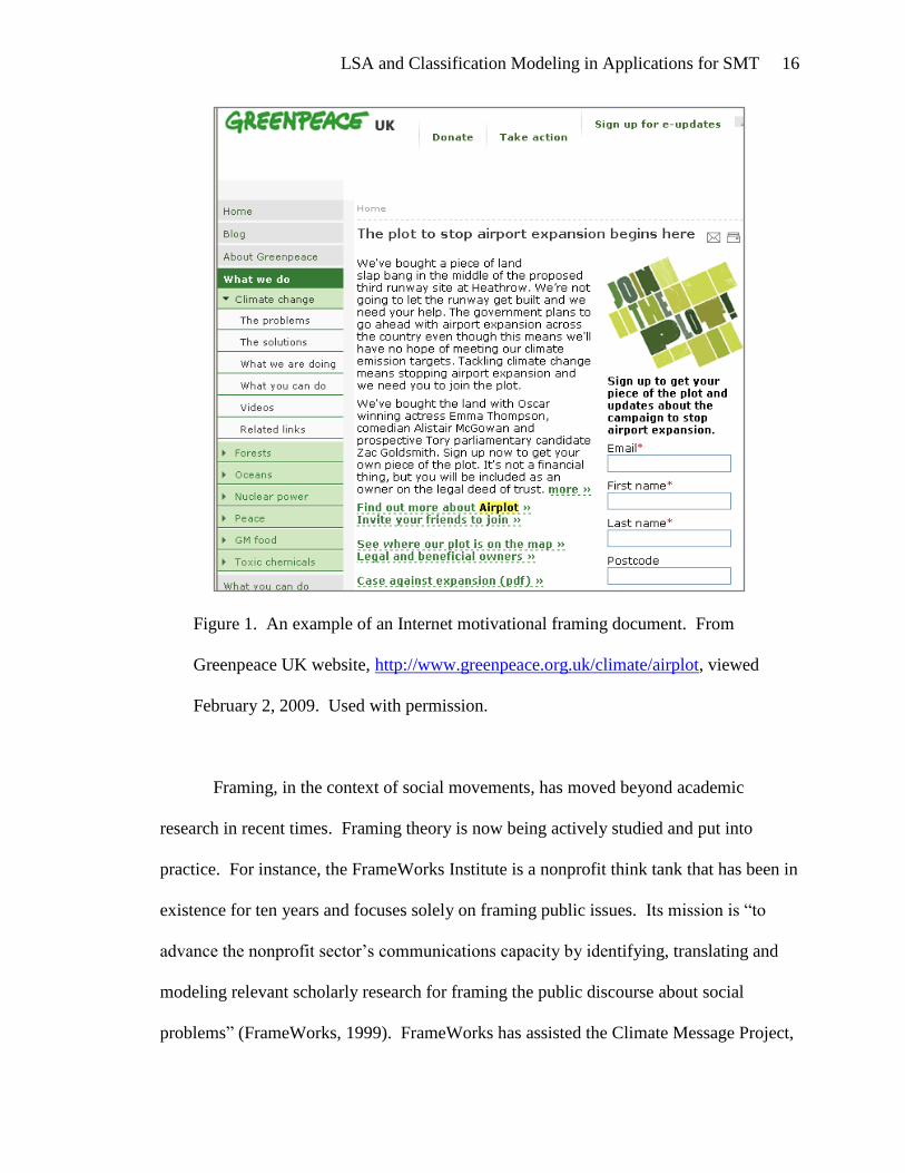
An example of motivational framing found on the Internet is shown in Figure 1.
This web page, obtained from the Greenpeace website and reproduced here with
permission, asks the reader to join an action to halt the expansion of Heathrow Airport.
Greenpeace, along with some celebrities, purchased a plot of land in the middle of the
proposed new runway at Heathrow. The reader is asked to sign up as an owner on the
legal deed of trust. Greenpeace wants to demonstrate the breadth of public support for its
position by obtaining as many owners as possible for this plot of land. Notice that,
toward the bottom of Figure 1, there is a link titled “Invite your friends to join.” This is
an effort to recruit more adherents to the cause. Figure 1 contains both text and images.
Images were not processed in this study, but the text can be extracted. The extracted text
then becomes a “document” which is subsequently processed and analyzed. The text in
Figure 1 is simply presented as an example and was not part of the corpus of documents
that were used in this study.
LSA and Classification Modeling in Applications for SMT 16
Figure 1. An example of an Internet motivational framing document. From
Greenpeace UK website, http://www.greenpeace.org.uk/climate/airplot, viewed
February 2, 2009. Used with permission.
Framing, in the context of social movements, has moved beyond academic
research in recent times. Framing theory is now being actively studied and put into
practice. For instance, the FrameWorks Institute is a nonprofit think tank that has been in
existence for ten years and focuses solely on framing public issues. Its mission is “to
advance the nonprofit sector‟s communications capacity by identifying, translating and
modeling relevant scholarly research for framing the public discourse about social
problems” (FrameWorks, 1999). FrameWorks has assisted the Climate Message Project,

LSA and Classification Modeling in Applications for SMT 17
a coalition of environmental SMOs in determining how to reframe the issue of global
warming (FrameWorks, n.d.).
Global Warming
Global warming has been selected as the social issue on which to base this study.
Global warming, sometimes referred to as climate change, is a contested topic. Various
factions debate whether or not the Earth is truly warming. Those that agree that the Earth
is experiencing an unprecedented period of warming argue among themselves over the
cause of that warming, the timing and effects of warming, and viable solutions to the
threat.
Concerns over the presumed effects of global warming have spawned social
movements that span cultural, religious, and geographical boundaries. This issue has
support from odd bedfellows like the Communist Party, which has published “Global
Warming – The Communist Solution” (Communist Party USA, 2008), and the Southern
Baptist Convention, which touts its own measures to combat global warming (Southern
Baptist Convention, 2007). From Australia (Climate Action Network Australia, 2008) to
Saudi Arabia (New Europe, 2008) the debate continues and global warming SMOs
abound.
Objectives
This study demonstrates a method to build classification models that can sift
through a corpus of documents, all of which are written on the topic of global warming,
and discover the small proportion of texts that are framing in nature. The purpose behind
these framing texts can range from attempts to sway public opinion regarding the issue to
LSA and Classification Modeling in Applications for SMT 18
recruiting persons to join organized efforts, such as protests or demonstrations, in order to
bring about desired change. The ability to deploy a model that can detect signs of such
activity, for instance by observing public Internet postings, could provide indications of
impending social conflict.
The social actions espoused by these framing documents could be harmless,
mildly disruptive, or in some cases could lead to violence. Global warming protests are
generally peaceful. In some cases, though, global warming protests have turned
disruptive or violent. At the EU-US Summit in June 2001, U.S. opposition to the Kyoto
Protocol set off protests in which environmentalists and anti-globalization activists threw
bottles and stones at Swedish riot police (BBC News, 2001). On two days in July 2008,
environmental protesters brought operations at the world‟s largest coal terminal to a
standstill by chaining themselves to a conveyor belt (Reuters, 2008). Regardless of
whether these social actions are peaceful or violent, early warning can aid communities
and law enforcement agencies in efforts to minimize the negative effects of expressed
social unrest.
This study does not address the issue itself, nor does it take a stand on the
controversy. Rather, this study takes advantage of the abundance of related documents
that have been produced in electronic form. Some of these are scientific publications,
studies, and news articles that are, or should be, objective and non-framing in nature.
Increasingly, the Internet is employed as the media of choice for disseminating social
activist views to the general public. The World Wide Web is a rich source of framing
documents that have been produced with the intent of influencing opinion on global
warming or recruiting others to join the efforts of the movement. For example, the

LSA and Classification Modeling in Applications for SMT 19
following motivational framing text was obtained from a site promoting a July 2008
climate rally in Australia.
Get serious! NO DESALINATION PLANT -- PHASE OUT COAL
NO NEW FREEWAY TUNNEL -- NO BAY DREDGING
YES to renewable energy, public transport & urgent action to stop global
warming.
We are calling for Victorians to join the Climate Emergency Rally
on July 5. We want to send a wake-up call to state and federal
governments that they are heading in the wrong direction. New coal, new
freeways and desalination plants increase our use of and reliance on fossil
fuels dramatically at a time when we must be cutting our use even more
dramatically. We are calling on governments to implement sustainable
alternatives to these irresponsible and expensive projects.
We call on all community groups and individuals to join us to send
this important message to the government. We are going to form a 140-
metre-long human sign to spell the words „Climate Emergency‟.
Please organise your group to send endorsement, tell everyone you
know, and come on the day wearing something red to symbolise
emergency. (Climate Rally, 2008)
The Climate Rally organizers were successful. The event was held in Melbourne,
Australia on July 5, 2008, with approximately 1,500 (police estimate) to 3,000-5,000

LSA and Classification Modeling in Applications for SMT 20
(organizers‟ estimate) in attendance. After listening to speakers and conducting a
peaceful march, the “Climate Emergency” sign (Figure 2) was formed by rally
participants. (Courtice, 2008) No violence was involved in this demonstration.
Figure 2. Photograph demonstrating the success of Climate Rally 2008 in
obtaining participants. (Campbell, 2008)
Methodology
This study employs a combination of Latent Semantic Analysis techniques and
statistical modeling algorithms (logistic regression, decision trees, and neural networks)
to produce models that accurately classify new, unseen text documents.
Latent Semantic Analysis (LSA) is a well established information retrieval
methodology that returns pertinent documents in response to a query (Deerwester,
Dumais, Furnas, Landauer, & Harshman, 1990). Perhaps the best known examples of
information retrieval applications are Internet search engines. LSA parses documents
from a corpus and represents the corpus as a matrix, most often with a row for each term
(word or phrase), a column for each document, and term counts or weights populating the

LSA and Classification Modeling in Applications for SMT 21
cells. Some analysts construct the matrix with rows representing documents and columns
representing terms, but in this study, the former representation is employed. The matrix
is known as a term-document matrix. It is sparse, meaning it has a large number of cells
with zero values for terms that do not appear in a particular document. The structure is a
high dimensional matrix, meaning there may be thousands of columns and tens of
thousands of rows.
LSA deals with the complexities of this large sparse matrix by employing singular
value decomposition (SVD) to reduce the dimensionality while retaining most of the
information in the corpus. SVD enables the calculation of a series of numerical values
for each text document. These calculated values can serve as input to classification
algorithms resulting in a tool that can accurately identify specific types of text, for
instance, the influential documents that are indicative of social action.
The first task in this study is to train a model to correctly classify framing and
non-framing documents. Second, a more specific classification model is developed to
further classify framing documents as belonging to one of the three main framing tasks:
diagnostic, prognostic, or motivational. Implementation of these techniques may open
the door to expanded research applications. For example, such applications might
monitor activist Internet postings and provide ongoing input for social scientists‟ study of
the dynamics of social movements.

LSA and Classification Modeling in Applications for SMT 22
RELATED RESEARCH
Employing LSA to generate predictive document attributes for classification
models is not new. For example, LSA has been applied in concert with the k-Nearest
Neighbors (kNN) algorithm to perform classification of topics in Reuters international
news reports (Naohiro, Murai, Yamada, & Bao, 2006). Also, the use of kNN and LSA
for document classification is not restricted to English. The same methods were used in a
study that classified Bulgarian news articles (Nakov, Valchanova, & Angelova, 2003). A
disadvantage of kNN is that it requires storage and processing of the training data to
accomplish classification of each new observation (Larose, 2005, p. 104). Rather than
using kNN, this study explores other classification algorithms which do not require a
large data store. Decision trees, logistic regression, and neural networks, as well as
ensemble modeling are considered. These algorithms can be trained to recognize a new
observation as belonging to one of a set of defined classes without requiring maintenance
of a large data store.
Classification of documents by framing tasks is a more difficult problem than
classifying news articles by subject. In this study, all documents address the same topic.
The models must detect more nebulous attributes such as motivation and intent. This
effort may be likened to classification by ideology. Different ideologies may be present
in documents that are written about a single topic. Ideological classification has been
successfully performed using singular value decomposition and a naïve Bayes classifier
to determine the party affiliation (Democrat or Republican) of Senators based on the text
of speeches made in the United States Senate (Morrow, Bader, Chew, & Speed, 2008).
LSA and Classification Modeling in Applications for SMT 23
Attributes that distinguish framing texts have been discussed extensively in Social
Movement Theory literature. A common approach is to develop a list of framing
keywords based on the most frequently occurring terms that are found in a collection of
framing documents (Triandafyllidou & Fotiou, 1998; Semetko & Valkenburg, 2000).
Computer-assisted qualitative data analysis software (CAQDAS) in conjunction with
word maps (electronic lists of words linked by associations) is another method that has
been proposed for identification of framing text (Koenig, 2005). Laborious processes
have also been used to characterize framing texts, such as manual extraction of words and
phrases which are then assigned codes for further analysis (Cooper, 2002). This is
effective, but expensive in terms of time and finances. It is also prone to issues of
human-induced bias and error.
The aforementioned methods as applied to framing texts have been utilized to
analyze processes and features of frame construction, rather than as a means to produce
input for classification models, which is the objective of this study. Examination of such
models can reveal additional insight into social movement frames. But, more notably, the
ability to develop framing classification models may extend theory into practice by
providing the means to monitor texts from various sources for indications of emerging or
escalating collective social actions.
LSA and Classification Modeling in Applications for SMT 24
METHODS
The processing of text for this study, including importation of documents, parsing,
singular value decomposition, and exploratory clustering, was performed using SAS®
Text Miner software (SAS® Text Miner, 2003-2005), a component of SAS® Enterprise
Miner™ (SAS® Enterprise Miner™, 2003-2005). Portions of the analysis utilized
SAS® and SAS/STAT® software (SAS® Software, 2002-2003). Additional analysis and
classification modeling used SPSS Clementine® (SPSS Clementine®, 2007).
The primary data mining task is classification of text documents, resulting in two
models. The first is dichotomous, classifying text documents as being either framing or
non-framing. The second, a polychotomous model, classifies text documents as one of
four types: diagnostic, prognostic, motivational, or non-framing. SAS® Text Miner
converts the information in the text into a structured form which can then be fed into
Clementine decision tree, logistic regression, and neural network algorithms for the
purpose of classification.
Collection of Electronic Text Documents
Publicly available text documents in electronic form, all addressing the topic of
global warming, were collected. Abstracts from technical papers, conference
presentations, and reviews (ISI Web of Knowledge, 2008) were assumed to be non-
framing documents. Framing texts were gathered from web sites that support various
social movements focused on the global warming issue. The framing texts were
annotated with the source web site URL, the date of access, and, as available, the Web
page date. A total of 6,531 framing and non-framing text documents were collected.
Examples of each type of document are shown in Appendix A.

LSA and Classification Modeling in Applications for SMT 25
Preprocessing of Text Documents
Document Classification
The documents that were analyzed in this study were obtained from abstracts of
journal papers, conference proceedings, news reports, text from web pages, or text
downloaded from web pages in the form of a pdf, a word processing document, or as text
contained within a spreadsheet. All documents in the corpus were classified by the
author as framing or non-framing. The framing documents were further classified, again
by the author, as belonging to one of three core framing tasks: diagnostic, prognostic, or
motivational (Snow & Benford, 1988). This classification was necessarily subjective;
however, every effort was made to faithfully adhere to the definitions of the three
framing tasks.
Some documents contained elements of all three framing tasks. An example of
this could be a web page that first mentions the dangers of global warming (diagnostic),
then goes on to say that legislation is needed to counteract the causes of global warming
(prognostic), and finally asks the reader to come and protest in front of the building
where legislators are preparing to vote on such legislation (motivational). When more
than one framing task was evident in a document, the document was classified by the task
that dominated the text. Distributions of documents by classification are shown in
Figures 3 and 4.
Figure 3. Distribution of documents by framing classification.
LSA and Classification Modeling in Applications for SMT 26
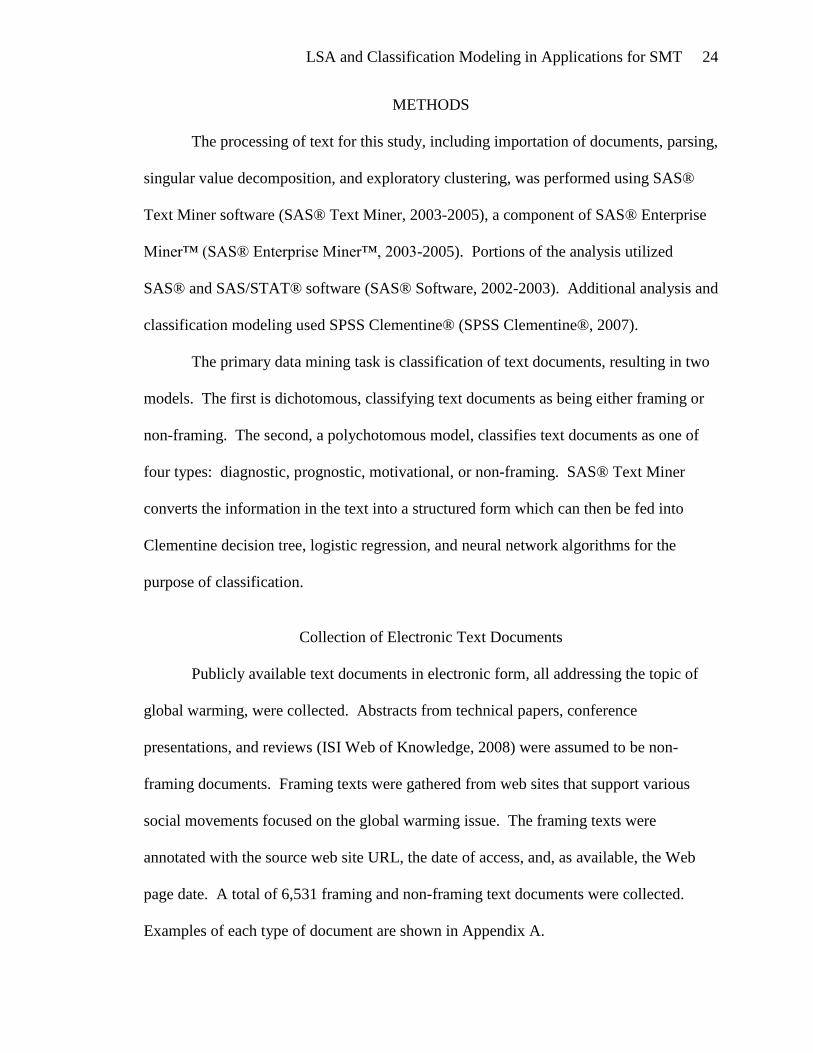
Figure 4. Distribution of documents by core framing task.
Removal of Personal Identifying Information
Names and all other personal identifying information were removed from the
framing documents since the focus of this study is on the analysis of text and not the
persons mentioned in the text.
Parsing the Text
Humans can process (e.g. read) text data in its raw, unstructured form. Processing
text by a computer, however, requires a series of steps to convert the words into a
numeric representation. The most basic representation is a count of the number of times
each word occurs in each document. Before the words can be counted, they must be
extracted from the documents. Parsing generally uses spaces and punctuation to separate
text into individual words.
After parsing out all the words that are found in a corpus, the term list may
contain tens of thousands of terms, some of which provide little value to the analysis.
Therefore parsing may also incorporate algorithms to exclude these extraneous terms.
The parsing process may be further refined by defining “terms.” A term is a distinct item
consisting of either a single word (e.g., “atmosphere,” “enact,” “important”) or a phrase
consisting of two or more words (e.g., “sea level,” “greenhouse gas emission,” “polar ice
cap”). SAS® Text Miner software provides a variety of parsing options. The options

LSA and Classification Modeling in Applications for SMT 27
selected for this study were: part of speech tagging, stemming, stop word list, and noun
phrases.
Part of Speech Tagging
Some words that are spelled identically may have different meanings depending
upon the part of speech. For example, consider the word “rose.” As a noun it refers to a
flower. As a verb it is the past tense of a word that means “to ascend.” As an adjective it
is a color that is pale red. Rose may also be a proper name for a woman. For this reason,
“rose” as a noun should be considered distinct from “rose” as a verb, and so on. Part of
speech tagging allows each of these four forms of “rose” to be processed individually in
order to maintain those distinctions. The number of occurrences of the verb “rose” in
each document is generated independently of the occurrences of the noun “rose” and each
is listed in the term list for the document collection. Without the part of speech
qualification, “rose” would appear once in the term list and the number of occurrences
would be the sum of occurrences of all forms of “rose.”
Stemming
In contrast to part of speech tagging, which keeps some words distinct even when
they are spelled identically, stemming combines all of the grammatical forms of a word
into one canonical form. In effect, stemming reduces the number of terms in the term list
and increases the accuracy by ensuring that multiple forms of a single word are not listed
separately.
Verbs are most often the target of stemming. The verb “go” has different
spellings for its tenses such as “gone,” “went,” and “going.” Stemming combines all
LSA and Classification Modeling in Applications for SMT 28
forms of this verb into the canonical form, “go.” SAS® Text Miner software precedes
the canonical form with a plus sign to indicate the presence of other forms.
Singular and plural forms of a noun are stemmed into the singular form. As with
verbs, SAS® Text Miner software indicates the presence of other forms by preceding the
singular noun with a plus sign.
Removal of Selected Terms
Some parts of speech are considered to be non-informative. For example,
conjunctions, such as “but,” “and,” “or,” are often placed in this category. While
grammatically useful, these words contribute little meaning to the text and can be
removed from the list of terms. The following parts of speech were removed from the
Global Warming corpus: Conjunction, Determiner, Auxiliary or Modal, Preposition,
Pronoun, Participle, Interjection, and Number. This leaves the following informative
parts of speech: Noun, Proper Noun, Verb, Adjective, Adverb, and Abbreviation.
Stemming and the removal of non-informative parts of speech are mechanized
methods that transform the list of terms into a smaller, more meaningful set. A stop word
list allows the analyst to manually specify additional deletions from the list of terms.
Stop words are terms that do not contribute meaning in the context of the analysis that is
being conducted. The determination of stop words should be carefully conducted in
concert with the goals of the researcher (Bilisoly, 2008, p. 245). A basic stop word list
was applied in this analysis. It contained 154 terms, such as “it,” “either,” and “this,” as
well as the individual letters of the alphabet.
LSA and Classification Modeling in Applications for SMT 29
Noun Phrases
Phrases are small groups of words that express a single idea. When certain
phrases occur repeatedly throughout the corpus of documents, the ideas represented by
those phrases may be captured by treating the entire phrase as a “term.” Counting
occurrences of “polar bear” and “polar ice cap” can be of more value in the analysis of
the corpus than counting the individual occurrences of “polar,” “bear,” “ice,” and “cap.”
The option in SAS® Text Miner software to identify noun phrases was selected in this
study.
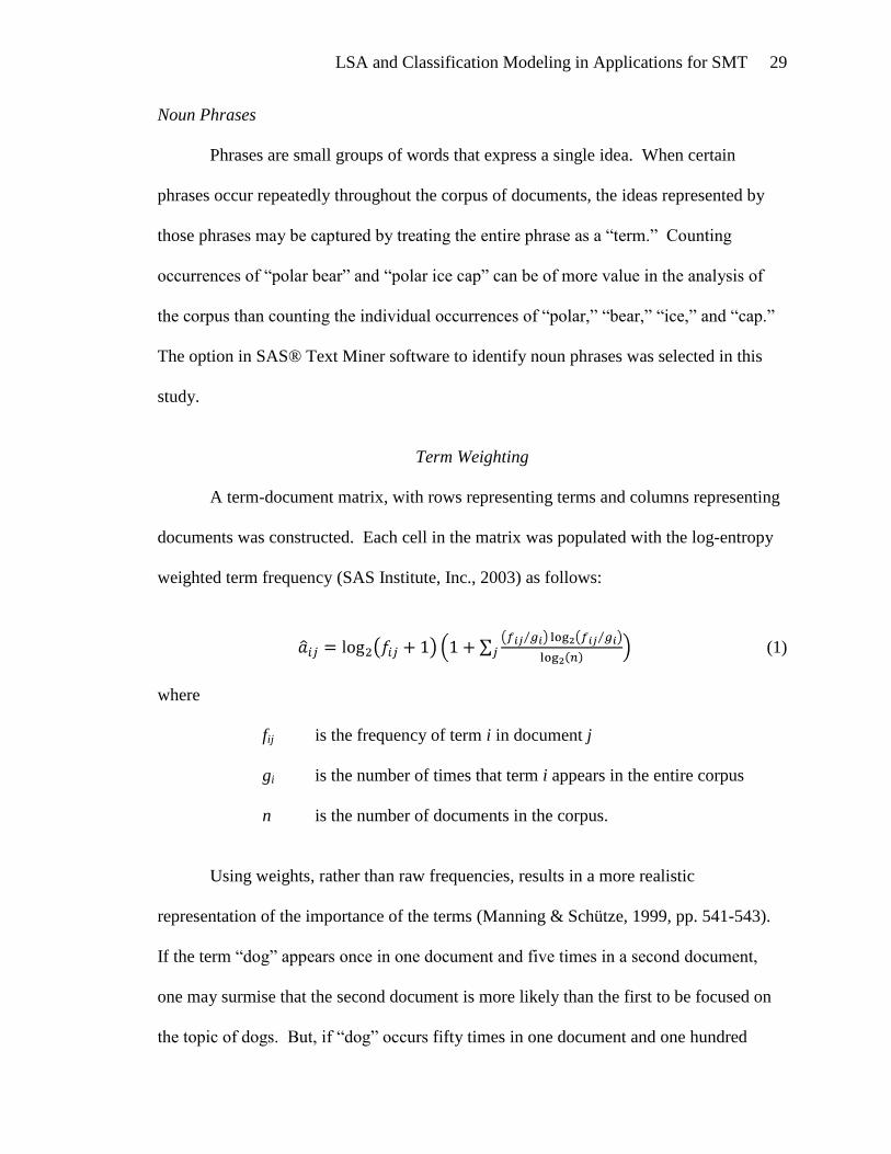
Term Weighting
A term-document matrix, with rows representing terms and columns representing
documents was constructed. Each cell in the matrix was populated with the log-entropy
weighted term frequency (SAS Institute, Inc., 2003) as follows:
(1)
where
fij is the frequency of term i in document j
gi is the number of times that term i appears in the entire corpus
n is the number of documents in the corpus.
Using weights, rather than raw frequencies, results in a more realistic
representation of the importance of the terms (Manning & Schütze, 1999, pp. 541-543).
If the term “dog” appears once in one document and five times in a second document,
one may surmise that the second document is more likely than the first to be focused on
the topic of dogs. But, if “dog” occurs fifty times in one document and one hundred
LSA and Classification Modeling in Applications for SMT 30
times in another document, those extra fifty occurrences in the second document do not
necessarily mean that the second document is twice as likely to be about dogs. In this,
admittedly extreme case, one would tend to state merely that both documents are
definitely about dogs. Logarithmic scaling of the term frequencies dampens the effect of
the higher counts, thus imparting a more reasonable measure of the term relevance.
Another important relation is obtained by incorporating the global frequency of
the term in the calculation of term weight. If the term “dog” appears frequently in many,
or all, of the documents, then that term will not be useful in distinguishing the documents
from one another. This is reflected in a lower term weight. This could be the case when
all documents in the corpus are about dog obedience training. If, however, the entire
corpus is about veterinary care for small pets and “dog” appears frequently in a small
number of documents, then “dog” will have a higher term weight. In this case, “dog” can
be of value when separating the documents by types of pets.
Singular Value Decomposition
This corpus of 6,531 documents contains over 23,000 terms after selecting only
the most informative parts of speech, applying a stop word list, and performing
stemming. The term-document matrix is quite sparse, meaning most cells contain zeroes.
This sparse, highly dimensional matrix cannot be processed efficiently or effectively.
Thus, singular value decomposition (SVD) is performed to transform the matrix into a
lower dimensional, compact form while still retaining most of the information
represented by the original matrix.
SVD decomposes a rectangular matrix into three matrices, which we shall refer to
as U, D, and V. The original matrix can be reconstructed by multiplication as UDVT. A
LSA and Classification Modeling in Applications for SMT 31
term-document matrix is more often than not rectangular since there are typically many
more terms than there are documents. The matrix U describes the original rows (terms)
as vectors of derived factor values. V describes the original columns (documents)
similarly. These factor values will be referred to as dimensions. D is a diagonal matrix
containing singular scaling values ordered from largest to smallest. In text mining, the
dimensionality is typically reduced by eliminating dimensions from U, D, and V,
beginning with the smallest values in D. When the dimensionality is reduced in this
manner, the reconstructed matrix, UDVT, is a least-squares best fit of the original matrix.
(Landauer, Foltz, & Laham, 1998)
For this study, only the first one hundred dimensions were calculated, giving a
truncated decomposition of the term-document matrix. Truncating to one hundred
dimensions is the default software setting and generally provides more than enough
information for classification modeling. In the truncated singular value decomposition of
the term-document matrix, the matrix VT contains a row for each document and a column
for each of the one hundred SVD dimensions. Now, rather than representing each
document as a vector of weights for tens of thousands of terms, each document is
represented as a vector in a space of one hundred dimensions. These one hundred SVD
dimension values for each document become the input variables for the classification
models.
The popularity of SVD in the field of text analytics is due to more than just its
ability to reduce dimensionality. The truncation of the decomposition addresses, at least
in part, the problem of synonymy (Manning, Raghavan, & Schütze, 2008, pp. 378-382).
Synonymy occurs when two or more different words have the same meaning, such as
LSA and Classification Modeling in Applications for SMT 32
“road” and “street.” Suppose we compare two document vectors that are composed of
term weights. One document contains the term “road” but not “street” and the other
document mentions “street” but not “road.” The term weight for “street” is zero in the
first document, as is the term weight for “road” in the second document. A calculation of
similarity between the two documents could rate the documents less similar than would a
human reader. Truncated SVD reflects similar co-occurrences of terms in the dimension
values and thus approximates the manner in which a human perceives similarity between
words (Landauer, Foltz, & Laham, 1998, p. 4).

LSA and Classification Modeling in Applications for SMT 33
Exploratory Data Analysis
The end result of the text preprocessing is a data set that contains a row for each
document and a column for each of the one hundred SVD dimensions. Each document is
now represented as a series of continuous numerical values. The first step in exploring
the corpus is to cluster the documents on the basis of the SVD dimension values. The
second step is exploration of the individual SVD dimensions as candidates for predictor
variables in the classification models.
SAS® Text Miner software provides two algorithms for clustering documents:
Expectation Maximization and Hierarchical. The documents in the Global Warming
corpus were clustered using Expectation Maximization with the SVD dimension values
serving as input variables. Twenty-one clusters were selected. Selection was an iterative
process beginning with thirteen clusters determined by the software. The documents
were then reclustered with the number of clusters specified by the analyst until the
twenty-one clusters were chosen. This set of clusters was the smallest set that clearly
represented distinct concepts.
For each cluster, SAS® Text Miner software returns a list of descriptive terms,
the number and proportion of documents, and the root mean squared standard deviation.
The descriptive terms for each cluster are the terms with the highest binomial
probabilities (SAS Institute, Inc., 2003). This calculation is defined in equation (2). The
clusters were profiled by consideration of the descriptive terms and occasional browsing
of individual documents that were assigned to each cluster. As a result of profiling, a
name was assigned to each cluster to identify its contents. The clusters are described in
detail in Appendix B.
LSA and Classification Modeling in Applications for SMT 34
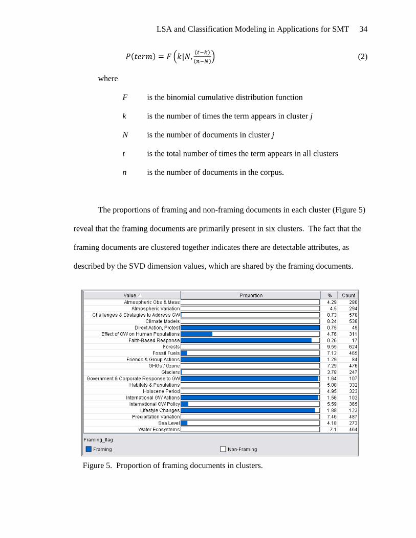
(2)
where
F is the binomial cumulative distribution function
k is the number of times the term appears in cluster j
N is the number of documents in cluster j
t is the total number of times the term appears in all clusters
n is the number of documents in the corpus.
The proportions of framing and non-framing documents in each cluster (Figure 5)
reveal that the framing documents are primarily present in six clusters. The fact that the
framing documents are clustered together indicates there are detectable attributes, as
described by the SVD dimension values, which are shared by the framing documents.
Figure 5. Proportion of framing documents in clusters.
LSA and Classification Modeling in Applications for SMT 35
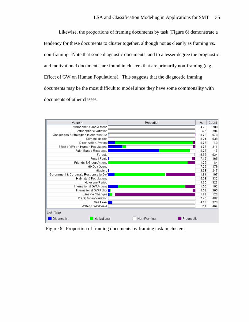
Likewise, the proportions of framing documents by task (Figure 6) demonstrate a
tendency for these documents to cluster together, although not as cleanly as framing vs.
non-framing. Note that some diagnostic documents, and to a lesser degree the prognostic
and motivational documents, are found in clusters that are primarily non-framing (e.g.
Effect of GW on Human Populations). This suggests that the diagnostic framing
documents may be the most difficult to model since they have some commonality with
documents of other classes.
Figure 6. Proportion of framing documents by framing task in clusters.
LSA and Classification Modeling in Applications for SMT 36
Preparation for Classification Modeling
Training and Test Data Sets
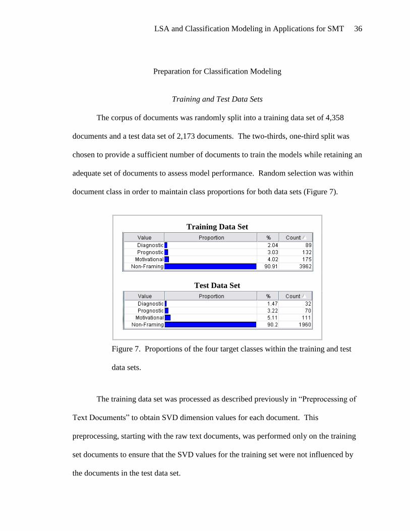
The corpus of documents was randomly split into a training data set of 4,358
documents and a test data set of 2,173 documents. The two-thirds, one-third split was
chosen to provide a sufficient number of documents to train the models while retaining an
adequate set of documents to assess model performance. Random selection was within
document class in order to maintain class proportions for both data sets (Figure 7).
Training Data Set
Test Data Set
Figure 7. Proportions of the four target classes within the training and test
data sets.
The training data set was processed as described previously in “Preprocessing of
Text Documents” to obtain SVD dimension values for each document. This
preprocessing, starting with the raw text documents, was performed only on the training
set documents to ensure that the SVD values for the training set were not influenced by
the documents in the test data set.
LSA and Classification Modeling in Applications for SMT 37
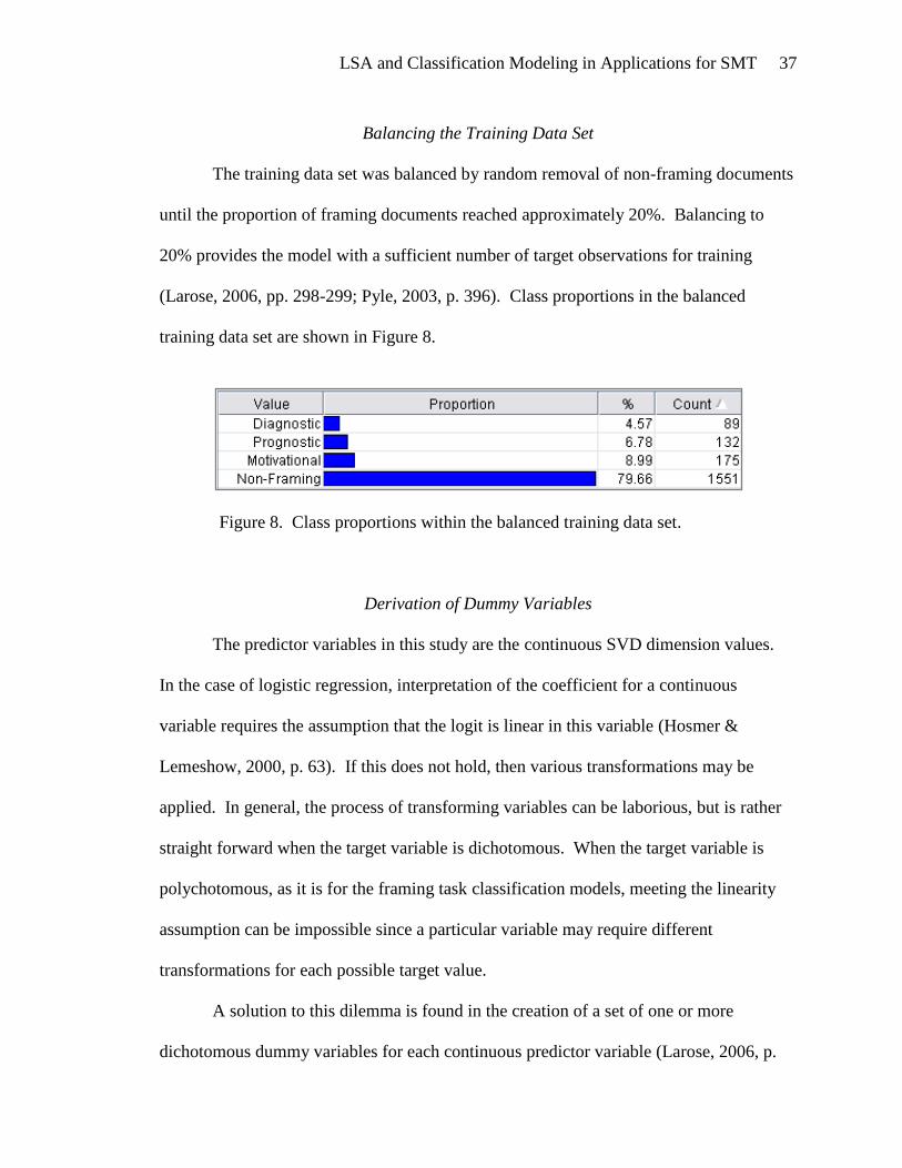
Balancing the Training Data Set
The training data set was balanced by random removal of non-framing documents
until the proportion of framing documents reached approximately 20%. Balancing to
20% provides the model with a sufficient number of target observations for training
(Larose, 2006, pp. 298-299; Pyle, 2003, p. 396). Class proportions in the balanced
training data set are shown in Figure 8.
Figure 8. Class proportions within the balanced training data set.
Derivation of Dummy Variables
The predictor variables in this study are the continuous SVD dimension values.
In the case of logistic regression, interpretation of the coefficient for a continuous
variable requires the assumption that the logit is linear in this variable (Hosmer &
Lemeshow, 2000, p. 63). If this does not hold, then various transformations may be
applied. In general, the process of transforming variables can be laborious, but is rather
straight forward when the target variable is dichotomous. When the target variable is
polychotomous, as it is for the framing task classification models, meeting the linearity
assumption can be impossible since a particular variable may require different
transformations for each possible target value.
A solution to this dilemma is found in the creation of a set of one or more
dichotomous dummy variables for each continuous predictor variable (Larose, 2006, p.
LSA and Classification Modeling in Applications for SMT 38
176). Each dummy variable is assigned a value of one if the predictor variable is within a
certain range, and zero otherwise. A form of bivariate analysis was employed to define
the number of dummy variables and their associated ranges for each continuous
predictor. This analysis reveals ranges of variable values for each SVD that are
positively, or negatively, associated with target variable values. This analysis also
reveals ranges of SVD values that display no relationship to the target variable values.
For some predictors, the bivariate analysis revealed little or no relationship between the
any values of the predictor and the target variable. In those cases, the predictor variables
were removed from consideration.
At this point, it should be noted that SVD variables are ordered such that SVD_1
explains more of the variance in the term document matrix than SVD_2, and so on. Thus,
one may expect that the higher ranked SVD variables, such as SVD_1 and SVD_2, will be
more effective predictors in a classification model. This was evident in the bivariate
analysis where SVD variables beyond SVD_35 displayed little relationship, positive or
negative with the target variables, so this analysis was discontinued after SVD_35.
The training data set was used for the bivariate analysis, to avoid the influence of
the documents that were set aside for testing. Initially, for each SVD variable, all
documents were binned into five percent intervals, meaning each interval encompassed a
range of SVD values such that approximately five percent of the documents in the corpus
had values within that range. This analysis was performed by coding a SAS® software
program which produced a table illustrating the relationship of each predictor variable
with the target variable.
LSA and Classification Modeling in Applications for SMT 39
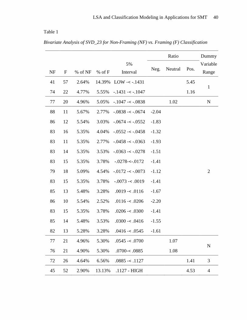
A set of these tables were produced for dichotomous target variables representing
each possible class: non-framing, diagnostic, prognostic, and motivational. Table 1
illustrates the bivariate analysis for the non-framing target variable and the SVD_23
continuous predictor variable, which is representative of the bivariate analysis performed
for all combinations of target and predictor variables. The ratios in the table are defined
as:
If (% of F) > (% of NF) then Ratio = (% of F) / (% of NF)
If (% of F) < (% of NF) then Ratio = - (% of NF) / (% of F)
where
NF is the number of non-framing documents in the 5% interval
F is the number of framing documents in the 5% interval
% of NF is the percent of non-framing documents from the training data set
(1,551 as shown in Figure 8) that are in the 5% interval.
% of F is the percent of framing documents from the training data set (396
as shown in Figure 8) that are in the 5% interval.
The horizontal solid lines define dummy variable ranges and were added to the
table by the analyst, as were the numbers “1” through “4” and the letters “N” which can
be seen on the right-hand side of Table 1. Four dummy variables were created for
SVD_23, one for each range of values labeled “1” through “4.” The letter “N” represents
a neutral interval, described in more detail below.
LSA and Classification Modeling in Applications for SMT 40
Table 1
Bivariate Analysis of SVD_23 for Non-Framing (NF) vs. Framing (F) Classification
NF F % of NF % of F
5%
Interval
Ratio Dummy
Variable
Range Neg. Neutral Pos.
41 57 2.64% 14.39% LOW -< -.1431 5.45 1
74 22 4.77% 5.55% -.1431 -< -.1047 1.16
77 20 4.96% 5.05% -.1047 -< -.0838 1.02 N
88 11 5.67% 2.77% -.0838 -< -.0674 -2.04
2
86 12 5.54% 3.03% -.0674 -< -.0552 -1.83
83 16 5.35% 4.04% -.0552 -< -.0458 -1.32
83 11 5.35% 2.77% -.0458 -< -.0363 -1.93
83 14 5.35% 3.53% -.0363 -< -.0278 -1.51
83 15 5.35% 3.78% -.0278-<-.0172 -1.41
79 18 5.09% 4.54% -.0172 -< -.0073 -1.12
83 15 5.35% 3.78% -.0073 -< .0019 -1.41
85 13 5.48% 3.28% .0019 -< .0116 -1.67
86 10 5.54% 2.52% .0116 -< .0206 -2.20
83 15 5.35% 3.78% .0206 -< .0300 -1.41
85 14 5.48% 3.53% .0300 -< .0416 -1.55
82 13 5.28% 3.28% .0416 -< .0545 -1.61
77 21 4.96% 5.30% .0545 -< .0700 1.07 N
76 21 4.90% 5.30% .0700-< .0885 1.08
72 26 4.64% 6.56% .0885 -< .1127 1.41 3
45 52 2.90% 13.13% .1127 - HIGH 4.53 4
LSA and Classification Modeling in Applications for SMT 41
The dummy variables are designed to capture ranges of SVD_23 that exhibit solid
positive (or negative) ratios between the two possible target values. Ratios within
approximately ±1.10 may be considered neutral. These intervals are labeled “N” and do
not require dummy variables. Neutral intervals are also used to separate adjacent positive
and negative intervals.
The SVD_23 dummy variables were calculated in Clementine “Derive” nodes and
were named SVD23_01, SVD23_02, SVD23_03, and SVD23_04. For example, the
derivation of SVD23_02 is:
if (SVD_23 >= -0.0838) and (SVD_23 < 0.0545) then
1
else
0
endif
In addition to allowing for the assumption of linearity in logistic regression, these
dummy variables generalize the information that is obtained from the original predictor
variable, thus reducing the risk of over-fitting a model. Rather than following the process
just described, dummy variables could be created from binning the predictor variables
into equal-sized bins. Many software packages, including Clementine, provide
convenient tools to do so. The method employed here, adapted from the author‟s
personal experience in credit risk modeling, requires additional time and effort, but
results in more meaningful dummy variables. Raymond Anderson, in his book on credit
LSA and Classification Modeling in Applications for SMT 42
scoring methods (Anderson, 2007, p. 358), outlines a similar process for defining dummy
variables in retail credit scoring. He recommends first creating fine classes consisting of
small, equal ranges for each predictor variable, and then combining those classes into
logical groupings that display similar risk. The fine and grouped classes correspond to
the 5% intervals and subsequent dummy variable ranges that were incorporated in this
analysis. Anderson further explains (2007, p. 359) the necessity for at least one neutral
interval containing classes that are near average risk, that have insufficient data, or that
do not logically fit with any of the defined dummy variables.
Two sets of dummy variables were calculated. The first set, listed in Appendix C,
was derived from the bivariate analysis of the SVD values and the non-framing target
variable. These dummy variables are intended for use in the first model, framing versus
non-framing classification.
The second set of dummy variables, described in Appendix D, was derived from
simultaneous consideration of the bivariate analysis for each of the framing classes. The
dummy variables in this second set are to be employed in the finer classification of
framing documents as belonging to one of the three framing tasks: diagnostic,
prognostic, or motivational. For this reason, intervals for each SVD variable were
defined to accommodate all three target variables.
LSA and Classification Modeling in Applications for SMT 43
Profiling Selected SVD Variables
The SVD variables are assigned rather nondescript names, SVD_1, SVD_2, etc.,
by the decomposition software. With some effort, an analyst can gain insight into the
nature of each SVD variable. In the course of developing classification models for this
study, two SVD variables were singled out as being particularly effective in the
classification models: SVD_2 and SVD_6. SVD_2 appeared to be very significant in
models which separate framing and non-framing documents. SVD_6 was important when
classifying documents by framing task. After model development was completed, these
two variables were profiled in order to understand why they were so important in the
final models. The profiling of these two variables is presented at this point in the paper in
order to provide the reader with additional understanding prior to the description of the
modeling process.
In the truncated singular value decomposition of the term-document matrix, the
matrix U contains a row for each term and a column for each of the one hundred SVD
dimensions. Thus, utilizing the U matrix, SVD dimension values are available for the
terms. These values, along with the bivariate analysis for each variable, are now used to
examine SVD_2 and SVD_6 in detail.
LSA and Classification Modeling in Applications for SMT 44
SVD_2
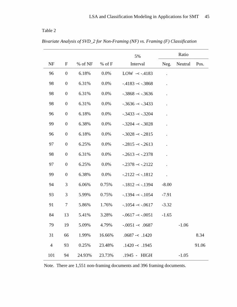
Analysis of SVD_2 clearly demonstrates a strong relationship between this
variable and the separation of framing and non-framing documents. The bivariate
analysis of documents for SVD_2 vs. the framing/non-framing target variable (Table 2)
shows that low values, less than -0.0051, of SVD_2 have a heavily negative association
with the framing class. From -0.0051 to 0.0687 SVD_2 is neutral. Above 0.0687 SVD_2
becomes increasingly positively associated with the framing class, except for the highest
values which are neutral.
So we may deduce that documents with a low SVD_2 value are more likely to be
non-framing and documents with higher SVD_2 values are likely to be framing. The
SVD_2 values for the documents appear to be an excellent indicator for framing vs. non-
framing documents.
LSA and Classification Modeling in Applications for SMT 45
Table 2
Bivariate Analysis of SVD_2 for Non-Framing (NF) vs. Framing (F) Classification
NF F % of NF % of F
5%
Interval
Ratio
Neg. Neutral Pos.
96 0 6.18% 0.0% LOW -< -.4183 .
98 0 6.31% 0.0% -.4183 -< -.3868 .
98 0 6.31% 0.0% -.3868 -< -.3636 .
98 0 6.31% 0.0% -.3636 -< -.3433 .
96 0 6.18% 0.0% -.3433 -< -.3204 .
99 0 6.38% 0.0% -.3204 -< -.3028 .
96 0 6.18% 0.0% -.3028 -< -.2815 .
97 0 6.25% 0.0% -.2815 -< -.2613 .
98 0 6.31% 0.0% -.2613 -< -.2378 .
97 0 6.25% 0.0% -.2378 -< -.2122 .
99 0 6.38% 0.0% -.2122 -< -.1812 .
94 3 6.06% 0.75% -.1812 -< -.1394 -8.00
93 3 5.99% 0.75% -.1394 -< -.1054 -7.91
91 7 5.86% 1.76% -.1054 -< -.0617 -3.32
84 13 5.41% 3.28% -.0617 -< -.0051 -1.65
79 19 5.09% 4.79% -.0051 -< .0687 -1.06
31 66 1.99% 16.66% .0687 -< .1420 8.34
4 93 0.25% 23.48% .1420 -< .1945 91.06
101 94 24.93% 23.73% .1945 - HIGH -1.05
Note. There are 1,551 non-framing documents and 396 framing documents.
LSA and Classification Modeling in Applications for SMT 46
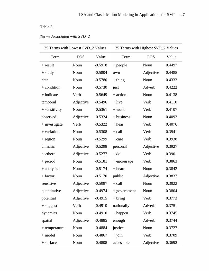
In order to discover the concepts represented by SVD_2, the terms associated with
SVD_2 must be inspected. Table 3 contains the terms that are most positively and most
negatively associated with SVD_2. A plus sign in front of a term indicates that term has
been stemmed. The terms associated with lower SVD_2 values appear to be analytic
(study, investigate, analysis), factual (result, data, observed, quantitative), and related to
climate change (condition, temporal, variation, climatic, temperature). None of the
terms in the list of the lowest SVD_2 values indicates passion or social involvement.
The terms associated with high SVD_2 values are quite different from those
associated with the lower values. These terms are social (people, own, personal),
emotional (care, heart, justice), and above all, these terms are action-oriented (action,
work, hear, call, do, encourage, bring, join). The objects of the actions are also evident
(business, public, government).
LSA and Classification Modeling in Applications for SMT 47
Table 3
Terms Associated with SVD_2
25 Terms with Lowest SVD_2 Values 25 Terms with Highest SVD_2 Values
Term POS Value Term POS Value
+ result Noun -0.5918 + people Noun 0.4497
+ study Noun -0.5804 own Adjective 0.4485
data Noun -0.5780 + thing Noun 0.4333
+ condition Noun -0.5730 just Adverb 0.4222
+ indicate Verb -0.5649 + action Noun 0.4138
temporal Adjective -0.5496 + live Verb 0.4110
+ sensitivity Noun -0.5361 + work Verb 0.4107
observed Adjective -0.5324 + business Noun 0.4092
+ investigate Verb -0.5322 + hear Verb 0.4076
+ variation Noun -0.5308 + call Verb 0.3941
+ region Noun -0.5299 + care Verb 0.3938
climatic Adjective -0.5298 personal Adjective 0.3927
northern Adjective -0.5277 + do Verb 0.3901
+ period Noun -0.5181 + encourage Verb 0.3863
+ analysis Noun -0.5174 + heart Noun 0.3842
+ factor Noun -0.5170 public Adjective 0.3837
sensitive Adjective -0.5087 + call Noun 0.3822
quantitative Adjective -0.4974 + government Noun 0.3804
potential Adjective -0.4915 + bring Verb 0.3773
+ suggest Verb -0.4910 nationally Adverb 0.3751
dynamics Noun -0.4910 + happen Verb 0.3745
spatial Adjective -0.4885 enough Adverb 0.3744
+ temperature Noun -0.4884 justice Noun 0.3727
+ model Noun -0.4867 + join Verb 0.3709
+ surface Noun -0.4808 accessible Adjective 0.3692
LSA and Classification Modeling in Applications for SMT 48
SVD_6
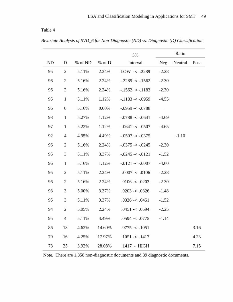
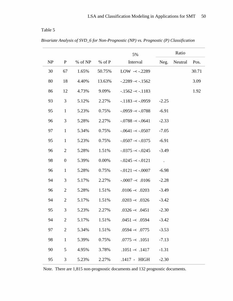
SVD_6 was singled out as the most important predictor variable by the two
models that were trained to discriminate between the three core framing tasks. The
bivariate analysis for SVD_6 suggests that diagnostic documents are negatively
associated with low values of SVD_6 and positively associated with high values of
SVD_6 (Table 4). In contrast, prognostic documents are positively associated with low
values of SVD_6 and negatively associated with high values of SVD_6 (Table 5).
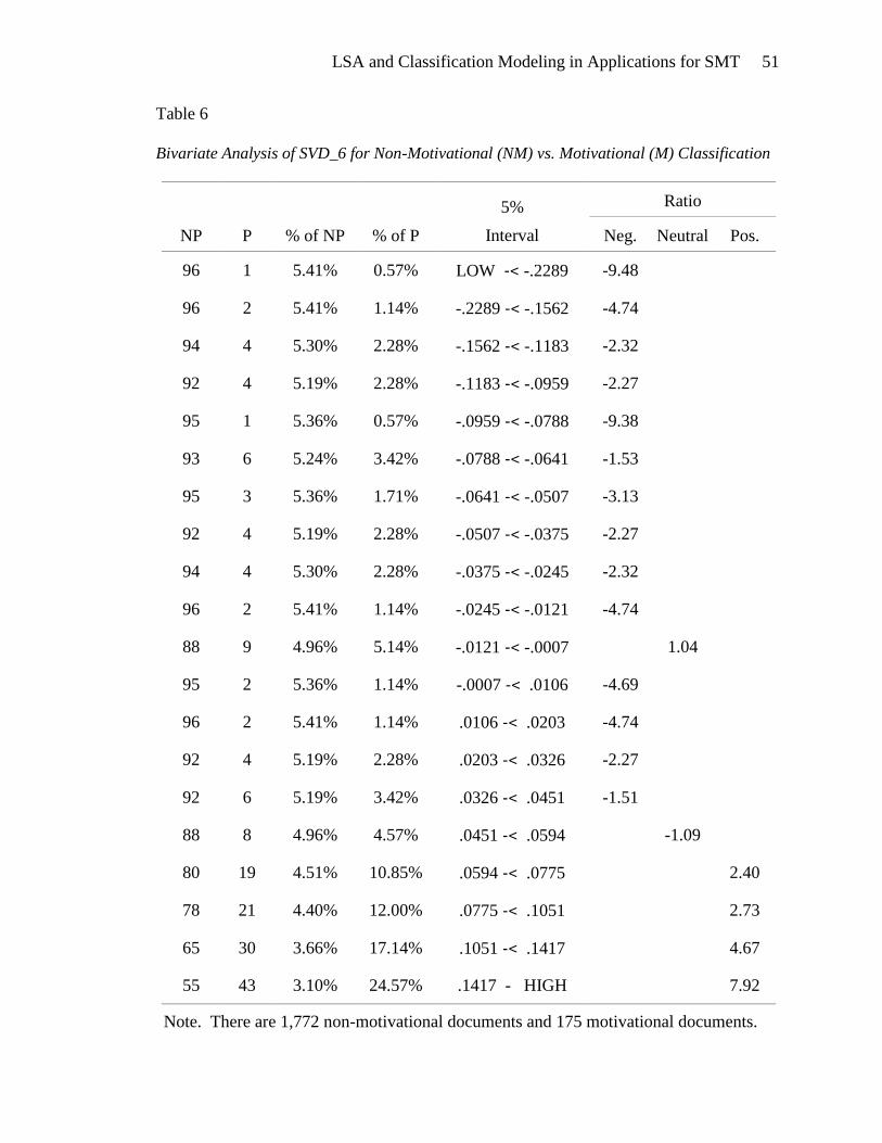
Motivational documents are negatively associated with low values and positively
associated with high values of SVD_6 (Table 6).
LSA and Classification Modeling in Applications for SMT 49
Table 4
Bivariate Analysis of SVD_6 for Non-Diagnostic (ND) vs. Diagnostic (D) Classification
ND D % of ND % of D
5%
Interval
Ratio
Neg. Neutral Pos.
95 2 5.11% 2.24% LOW -< -.2289 -2.28
96 2 5.16% 2.24% -.2289 -< -.1562 -2.30
96 2 5.16% 2.24% -.1562 -< -.1183 -2.30
95 1 5.11% 1.12% -.1183 -< -.0959 -4.55
96 0 5.16% 0.00% -.0959 -< -.0788 .
98 1 5.27% 1.12% -.0788 -< -.0641 -4.69
97 1 5.22% 1.12% -.0641 -< -.0507 -4.65
92 4 4.95% 4.49% -.0507 -< -.0375 -1.10
96 2 5.16% 2.24% -.0375 -< -.0245 -2.30
95 3 5.11% 3.37% -.0245 -< -.0121 -1.52
96 1 5.16% 1.12% -.0121 -< -.0007 -4.60
95 2 5.11% 2.24% -.0007 -< .0106 -2.28
96 2 5.16% 2.24% .0106 -< .0203 -2.30
93 3 5.00% 3.37% .0203 -< .0326 -1.48
95 3 5.11% 3.37% .0326 -< .0451 -1.52
94 2 5.05% 2.24% .0451 -< .0594 -2.25
95 4 5.11% 4.49% .0594 -< .0775 -1.14
86 13 4.62% 14.60% .0775 -< .1051 3.16
79 16 4.25% 17.97% .1051 -< .1417 4.23
73 25 3.92% 28.08% .1417 - HIGH 7.15
Note. There are 1,858 non-diagnostic documents and 89 diagnostic documents.
LSA and Classification Modeling in Applications for SMT 50
Table 5
Bivariate Analysis of SVD_6 for Non-Prognostic (NP) vs. Prognostic (P) Classification
NP P % of NP % of P
5%
Interval
Ratio
Neg. Neutral Pos.
30 67 1.65% 50.75% LOW -< -.2289 30.71
80 18 4.40% 13.63% -.2289 -< -.1562 3.09
86 12 4.73% 9.09% -.1562 -< -.1183 1.92
93 3 5.12% 2.27% -.1183 -< -.0959 -2.25
95 1 5.23% 0.75% -.0959 -< -.0788 -6.91
96 3 5.28% 2.27% -.0788 -< -.0641 -2.33
97 1 5.34% 0.75% -.0641 -< -.0507 -7.05
95 1 5.23% 0.75% -.0507 -< -.0375 -6.91
96 2 5.28% 1.51% -.0375 -< -.0245 -3.49
98 0 5.39% 0.00% -.0245 -< -.0121 .
96 1 5.28% 0.75% -.0121 -< -.0007 -6.98
94 3 5.17% 2.27% -.0007 -< .0106 -2.28
96 2 5.28% 1.51% .0106 -< .0203 -3.49
94 2 5.17% 1.51% .0203 -< .0326 -3.42
95 3 5.23% 2.27% .0326 -< .0451 -2.30
94 2 5.17% 1.51% .0451 -< .0594 -3.42
97 2 5.34% 1.51% .0594 -< .0775 -3.53
98 1 5.39% 0.75% .0775 -< .1051 -7.13
90 5 4.95% 3.78% .1051 -< .1417 -1.31
95 3 5.23% 2.27% .1417 - HIGH -2.30
Note. There are 1,815 non-prognostic documents and 132 prognostic documents.
LSA and Classification Modeling in Applications for SMT 51
Table 6
Bivariate Analysis of SVD_6 for Non-Motivational (NM) vs. Motivational (M) Classification
NP P % of NP % of P
5%
Interval
Ratio
Neg. Neutral Pos.
96 1 5.41% 0.57% LOW -< -.2289 -9.48
96 2 5.41% 1.14% -.2289 -< -.1562 -4.74
94 4 5.30% 2.28% -.1562 -< -.1183 -2.32
92 4 5.19% 2.28% -.1183 -< -.0959 -2.27
95 1 5.36% 0.57% -.0959 -< -.0788 -9.38
93 6 5.24% 3.42% -.0788 -< -.0641 -1.53
95 3 5.36% 1.71% -.0641 -< -.0507 -3.13
92 4 5.19% 2.28% -.0507 -< -.0375 -2.27
94 4 5.30% 2.28% -.0375 -< -.0245 -2.32
96 2 5.41% 1.14% -.0245 -< -.0121 -4.74
88 9 4.96% 5.14% -.0121 -< -.0007 1.04
95 2 5.36% 1.14% -.0007 -< .0106 -4.69
96 2 5.41% 1.14% .0106 -< .0203 -4.74
92 4 5.19% 2.28% .0203 -< .0326 -2.27
92 6 5.19% 3.42% .0326 -< .0451 -1.51
88 8 4.96% 4.57% .0451 -< .0594 -1.09
80 19 4.51% 10.85% .0594 -< .0775 2.40
78 21 4.40% 12.00% .0775 -< .1051 2.73
65 30 3.66% 17.14% .1051 -< .1417 4.67
55 43 3.10% 24.57% .1417 - HIGH 7.92
Note. There are 1,772 non-motivational documents and 175 motivational documents.
LSA and Classification Modeling in Applications for SMT 52
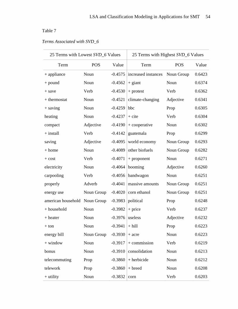
Investigation of the terms associated with SVD_6 (Table 7) should give more
insight into its relationship with the framing task classifications. The bivariate analyses
of SVD_6 showed that prognostic documents are positively associated with low SVD_6
values in contrast with diagnostic and motivational documents which are negatively
associated with low SVD_6 values. This association is quite apparent from observing the
twenty five terms with the lowest SVD_6 values. These terms are indicative of solutions
to global warming such as reducing home energy consumption and options to reduce
driving one‟s personal vehicle.
The positive association of high SVD_6 values with diagnostic and motivational
documents, as indicated by the bivariate analyses, is not immediately apparent from
perusal of the twenty five terms that have the highest SVD_6 values. The terms protest
and bandwagon, which could occur in motivational documents, are present in this list.
Climate changing and Guatemala could be indicative of diagnostic documents.
Apparently, more than just twenty five terms should be analyzed for the high SVD_6
values. The SVD_6 bivariate analyses show that diagnostic and motivational documents
are most positively associated with SVD_6 values that are 0.1417 and greater. There are
over 600 terms in that interval, which are listed in Appendix E.
Terms highlighted in yellow in Appendix E appear to be motivational. These
terms include types of actions: tough action, global action, urgent action, real action,
international action, and future action. There are verbs and phrases defining the activity:
lobby, act, commit, send, fight, gather, and win. Events can be found in this list: protest,
meeting, training, strategy sessions, and rally. The emotional appeal for action is also
evident: exciting, urgently, anger, and alarm. And finally, the hallmark of a

LSA and Classification Modeling in Applications for SMT 53
motivational document is the emphasis on people gathering together to take action:
bandwagon, group, movement, organize, mobilize, global movement, and friends. The
presence of these terms in the list of terms associated with high SVD_6 values gives
credence to the usefulness of SVD_6 in distinguishing motivational framing documents.
Terms that seem to be diagnostic are highlighted in green in Appendix E.
Diagnostic documents define a problem, often place blame and identify victims and
consequences. The problem definition is seen in the presence of terms such as: climate
change, climate-changing, climate crisis, rising sea levels, danger, devastating, drastic
increase, environmental destruction, and dangerous climate change. Placing blame is
indicated by the terms: polluter, rich countries, oil giant, foreign oil, aviation emissions,
interest-group, and corporation. Victims are also abundant in the list of terms: aquatic
life, women, coastal regions, human health, low-income, poor, amazon, mangrove forest,
wildlife, and rainforest. The association of these terms with high SVD_6 values validates
the usefulness of SVD_6 for identifying diagnostic framing documents.
LSA and Classification Modeling in Applications for SMT 54
Table 7
Terms Associated with SVD_6
25 Terms with Lowest SVD_6 Values 25 Terms with Highest SVD_6 Values
Term POS Value Term POS Value
+ appliance Noun -0.4575 increased instances Noun Group 0.6423
+ pound Noun -0.4562 + giant Noun 0.6374
+ save Verb -0.4530 + protest Verb 0.6362
+ thermostat Noun -0.4521 climate-changing Adjective 0.6341
+ saving Noun -0.4259 bbc Prop 0.6305
heating Noun -0.4237 + cite Verb 0.6304
compact Adjective -0.4190 + cooperative Noun 0.6302
+ install Verb -0.4142 guatemala Prop 0.6299
saving Adjective -0.4095 world economy Noun Group 0.6293
+ home Noun -0.4089 other biofuels Noun Group 0.6282
+ cost Verb -0.4071 + proponent Noun 0.6271
electricity Noun -0.4064 booming Adjective 0.6260
carpooling Verb -0.4056 bandwagon Noun 0.6251
properly Adverb -0.4041 massive amounts Noun Group 0.6251
energy use Noun Group -0.4020 corn ethanol Noun Group 0.6251
american household Noun Group -0.3983 political Prop 0.6248
+ household Noun -0.3982 + price Verb 0.6237
+ heater Noun -0.3976 useless Adjective 0.6232
+ ton Noun -0.3941 + hill Prop 0.6223
energy bill Noun Group -0.3930 + acre Noun 0.6223
+ window Noun -0.3917 + commission Verb 0.6219
bonus Noun -0.3910 consolidation Noun 0.6213
telecommuting Prop -0.3860 + herbicide Noun 0.6212
telework Prop -0.3860 + breed Noun 0.6208
+ utility Noun -0.3832 corn Verb 0.6203
LSA and Classification Modeling in Applications for SMT 55
Modeling Algorithms
Several modeling algorithms are incorporated in this study. CART, logistic
regression, and neural network models were developed for both the framing/non-framing
model (Model 1) and the non-framing/diagnostic/prognostic/motivational model (Model
2). In addition, the results of these modeling algorithms were incorporated into
combination (ensemble) models. A brief discussion of each modeling method follows.
CART Algorithm
Classification and Regression Trees (CART) are a type of decision tree, which
begin with a root node which contains all observations in the data set. The predictor
variables are tested to determine the best manner in which to split the root node
observations into two or more nodes that distinguish the classes. These nodes are placed
below the root node and the process is repeated, building a structure that looks more like
a root system than a tree. The final nodes are called leaf nodes.
The CART method (Breiman, Friedman, Olshen, & Stone, 1984) is a decision tree
algorithm in which each node is split into just two branches. The upper node is referred
to as the parent node and the two nodes beneath each parent node are called child nodes.
The target variable must be discrete, consisting of a finite set of classes. The predictor
variables may be categorical or continuous. Beginning with the root node, the tree grows
by successively splitting each node into two child nodes until a prescribed stopping
criterion is met. The objective is to end up with leaf nodes that are as pure as possible,
meaning these nodes each contain as high of a proportion of observations belonging to
one class as possible.
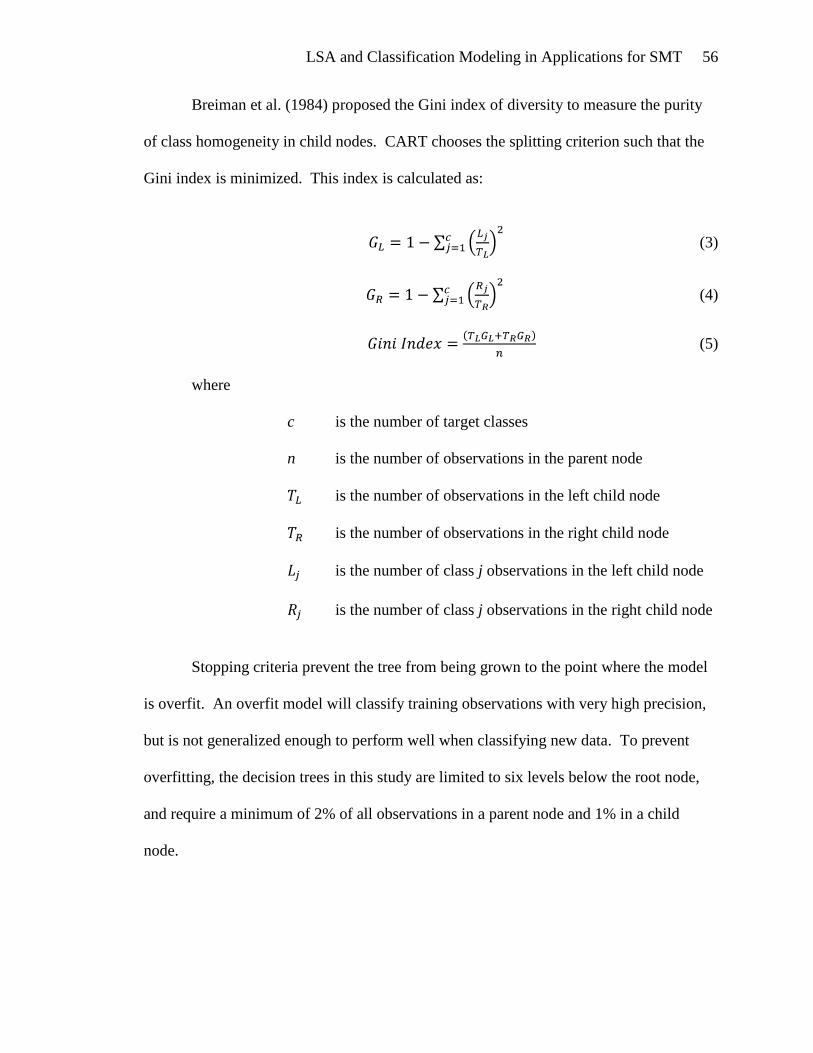
LSA and Classification Modeling in Applications for SMT 56
Breiman et al. (1984) proposed the Gini index of diversity to measure the purity
of class homogeneity in child nodes. CART chooses the splitting criterion such that the
Gini index is minimized. This index is calculated as:
(3)
(4)
(5)
where
c is the number of target classes
n is the number of observations in the parent node
is the number of observations in the left child node
is the number of observations in the right child node
is the number of class j observations in the left child node
is the number of class j observations in the right child node
Stopping criteria prevent the tree from being grown to the point where the model
is overfit. An overfit model will classify training observations with very high precision,
but is not generalized enough to perform well when classifying new data. To prevent
overfitting, the decision trees in this study are limited to six levels below the root node,
and require a minimum of 2% of all observations in a parent node and 1% in a child
node.
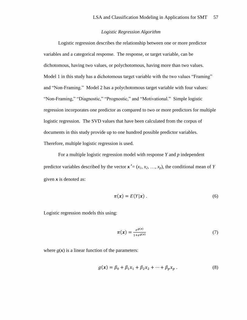
LSA and Classification Modeling in Applications for SMT 57
Logistic Regression Algorithm
Logistic regression describes the relationship between one or more predictor
variables and a categorical response. The response, or target variable, can be
dichotomous, having two values, or polychotomous, having more than two values.
Model 1 in this study has a dichotomous target variable with the two values “Framing”
and “Non-Framing.” Model 2 has a polychotomous target variable with four values:
“Non-Framing,” “Diagnostic,” “Prognostic,” and “Motivational.” Simple logistic
regression incorporates one predictor as compared to two or more predictors for multiple
logistic regression. The SVD values that have been calculated from the corpus of
documents in this study provide up to one hundred possible predictor variables.
Therefore, multiple logistic regression is used.
For a multiple logistic regression model with response Y and p independent
predictor variables described by the vector x’ = (x1, x2, …, xp), the conditional mean of Y
given x is denoted as:
. (6)
Logistic regression models this using:
(7)
where g(x) is a linear function of the parameters:
. (8)

LSA and Classification Modeling in Applications for SMT 58
Note that equation (7) implies that
(9)
This is called the logit transformation. The logistic regression parameters, β’ = (β0, β1,
…, βp) are estimated by maximum likelihood estimation. The log likelihood function is
expressed as:
(10)
Differentiating L(β|x) with respect to each parameter, setting the result equal to zero, and
solving generates the maximum likelihood estimator.
Neural Network Algorithm
Artificial Neural Networks, or simply neural networks, are simplified models of
biological nervous systems such as the human brain. A biological neuron collects
information from other neurons through dendrites. The neuron processes the information
and fires when a threshold is attained, sending information through an axon to other
neurons.
A neural network is composed of layers that correspond to the neuron functions.
The input layer consists of a node for each predictor, which is connected to one or more
hidden layers, the last of which connects to an output layer having one or more nodes. If
the target variable is dichotomous or consists of ordered classes, then one output node
may be tested against threshold values to determine the classification. When the target
variable consists of multiple unordered classes, the output layer will contain one node for
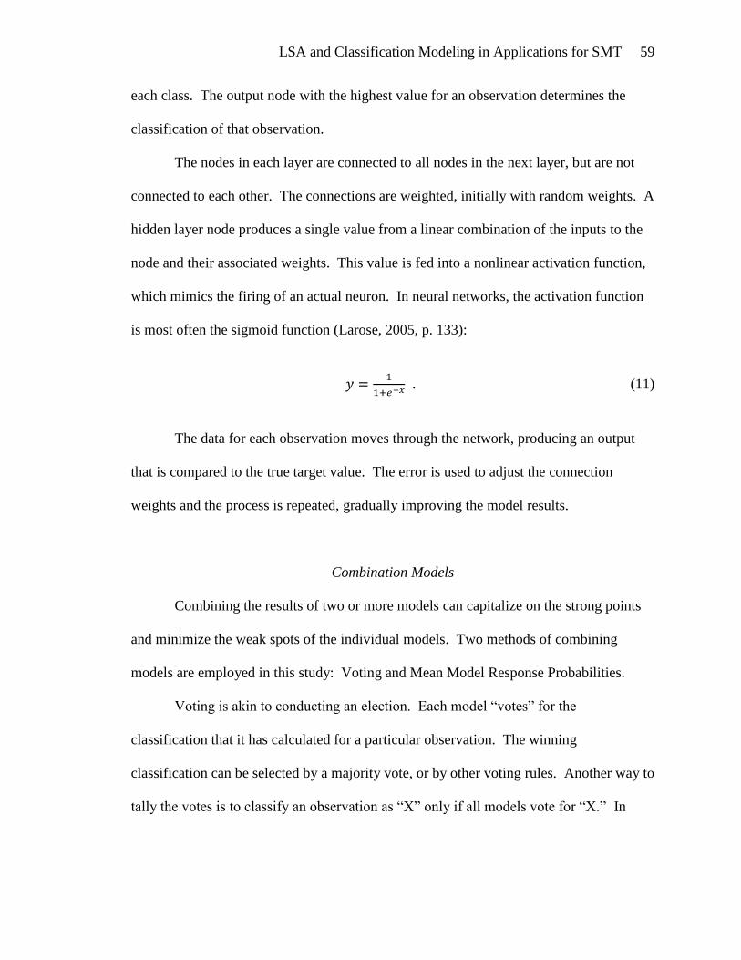
LSA and Classification Modeling in Applications for SMT 59
each class. The output node with the highest value for an observation determines the
classification of that observation.
The nodes in each layer are connected to all nodes in the next layer, but are not
connected to each other. The connections are weighted, initially with random weights. A
hidden layer node produces a single value from a linear combination of the inputs to the
node and their associated weights. This value is fed into a nonlinear activation function,
which mimics the firing of an actual neuron. In neural networks, the activation function
is most often the sigmoid function (Larose, 2005, p. 133):
. (11)
The data for each observation moves through the network, producing an output
that is compared to the true target value. The error is used to adjust the connection
weights and the process is repeated, gradually improving the model results.
Combination Models
Combining the results of two or more models can capitalize on the strong points
and minimize the weak spots of the individual models. Two methods of combining
models are employed in this study: Voting and Mean Model Response Probabilities.
Voting is akin to conducting an election. Each model “votes” for the
classification that it has calculated for a particular observation. The winning
classification can be selected by a majority vote, or by other voting rules. Another way to
tally the votes is to classify an observation as “X” only if all models vote for “X.” In
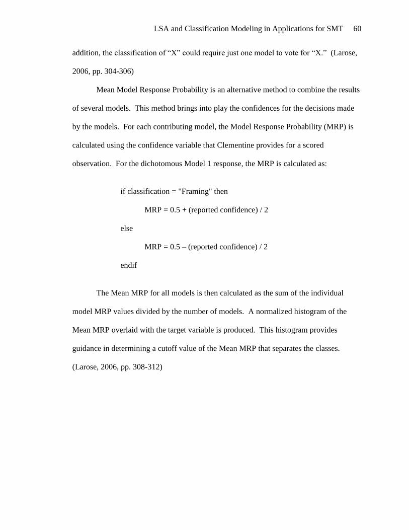
LSA and Classification Modeling in Applications for SMT 60
addition, the classification of “X” could require just one model to vote for “X.” (Larose,
2006, pp. 304-306)
Mean Model Response Probability is an alternative method to combine the results
of several models. This method brings into play the confidences for the decisions made
by the models. For each contributing model, the Model Response Probability (MRP) is
calculated using the confidence variable that Clementine provides for a scored
observation. For the dichotomous Model 1 response, the MRP is calculated as:
if classification = "Framing" then
MRP = 0.5 + (reported confidence) / 2
else
MRP = 0.5 – (reported confidence) / 2
endif
The Mean MRP for all models is then calculated as the sum of the individual
model MRP values divided by the number of models. A normalized histogram of the
Mean MRP overlaid with the target variable is produced. This histogram provides
guidance in determining a cutoff value of the Mean MRP that separates the classes.
(Larose, 2006, pp. 308-312)

LSA and Classification Modeling in Applications for SMT 61
Evaluation Metrics
The models in this study are designed to discover small numbers of interesting
(framing) documents that are buried within a collection of mostly uninteresting (non-
framing) documents. For traditional measures of error, the large number of non-framing
documents will have a disproportionate influence in communicating the effectiveness of
the model. Intuitively one does not mind if a few uninteresting documents are included
when a model plucks framing documents from a large mass of texts, as long as most of
the interesting documents are found. However, if those few uninteresting documents
become numerous, they thwart the intentions behind developing a classification model in
the first place. Four measures, precision, recall, F1 measure, and accuracy, reflect these
points of view and are often used to evaluate models that deal with text (Manning,
Raghavan, & Schütze, 2008, pp. 142-144). These are the metrics that will serve to
evaluate the models that are developed in this study.
For the framing/non-framing classification, precision is the proportion of framing
documents that truly are framing out of all documents classified as framing by the model.
Recall is the proportion of framing documents that were correctly identified by the model
out of all framing documents that exist in the data set. The balanced F1 measure is the
equally weighted harmonic mean of precision and recall. Accuracy is the proportion of
correctly classified documents. These metrics are defined as:
(12)
(13)

LSA and Classification Modeling in Applications for SMT 62
(14)
(15)
The non-framing/diagnostic/prognostic/motivational model requires a slight
modification to the four metrics. Precision, recall, F1 measure, and accuracy are
calculated individually for each of the four classes as if there were a separate confusion
matrix for each class (e.g. motivational versus not motivational). Overall precision,
recall, F1 measure, and accuracy are then calculated.
For a polychotomous target variable, there are two methods for calculating overall
precision, recall, F1 measure, and accuracy. Macro-averaging calculates the average of
the individual evaluation measures over all classes. For example, the macro-averaged
precision is equal to the sum of the non-framing precision, the diagnostic precision, the
prognostic precision, and the motivational precision, divided by four. Micro-averaging
creates one large confusion matrix, and then calculates accuracy over the entire table. In
situations where the classes contain similar numbers of observations, the results from
these two methods are comparable. When the number of documents varies greatly
between classes, as it does in this study (non-framing is much larger than the other three
classes), the large classes dominate micro-averaging results. To avoid this effect, macro-
averaging will be employed to evaluate overall model precision, recall, F1 measure, and
accuracy for the polychotomous target variables.

LSA and Classification Modeling in Applications for SMT 63
Model 1: Framing/Non-Framing Classification
The goal of Model 1 is to accurately separate framing texts from non-framing
texts. A variety of modeling algorithms (CART, logistic regression, and neural network)
were employed using continuous or dummy predictor variables. Two target variables
were calculated for Model 1: Framing_Name, a dichotomous string variable with the
values “Framing” or “Non-Framing,” and NON_FRAMING, a dichotomous integer
variable with the value 1 indicating a non-framing document or 0 indicating a framing
document. These target variables portray the same information, but provide the option of
using a string or numeric target at the discretion of the modeler.
CART Model 1
Training: CART Model 1
Decision trees are not adversely affected by non-linear predictor variables. Thus,
both the continuous SVD variables and the calculated SVD dummy variables are
candidates for CART predictors. A CART model can use categorical target variables that
are either numeric or string. Either of the Model 1 target variables would be acceptable
to the CART algorithm and would generate equivalent results. Framing_Name was
chosen as the target variable because it is more descriptive.
Two CART models were developed. One used the SVD dummy variables listed
in Appendix C as predictor variables. The other used the continuous SVD variables,
SVD_1 through SVD_100 as predictor variables. Both models were trained using the
balanced training set of documents.
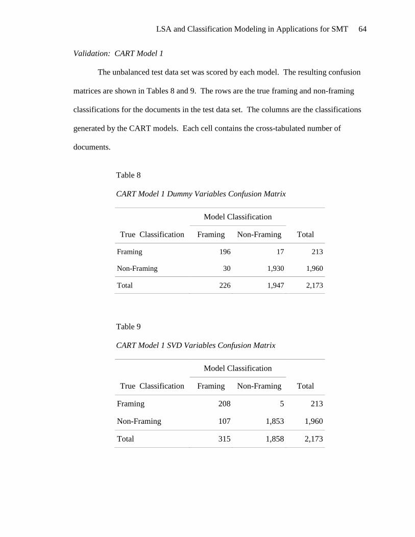
LSA and Classification Modeling in Applications for SMT 64
Validation: CART Model 1
The unbalanced test data set was scored by each model. The resulting confusion
matrices are shown in Tables 8 and 9. The rows are the true framing and non-framing
classifications for the documents in the test data set. The columns are the classifications
generated by the CART models. Each cell contains the cross-tabulated number of
documents.
Table 8
CART Model 1 Dummy Variables Confusion Matrix
True Classification
Model Classification
Total Framing Non-Framing
Framing 196 17 213
Non-Framing 30 1,930 1,960
Total 226 1,947 2,173
Table 9
CART Model 1 SVD Variables Confusion Matrix
True Classification
Model Classification
Total Framing Non-Framing
Framing 208 5 213
Non-Framing 107 1,853 1,960
Total 315 1,858 2,173
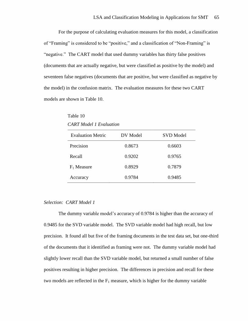
LSA and Classification Modeling in Applications for SMT 65
For the purpose of calculating evaluation measures for this model, a classification
of “Framing” is considered to be “positive,” and a classification of “Non-Framing” is
“negative.” The CART model that used dummy variables has thirty false positives
(documents that are actually negative, but were classified as positive by the model) and
seventeen false negatives (documents that are positive, but were classified as negative by
the model) in the confusion matrix. The evaluation measures for these two CART
models are shown in Table 10.
Table 10
CART Model 1 Evaluation
Evaluation Metric DV Model SVD Model
Precision 0.8673 0.6603
Recall 0.9202 0.9765
F1 Measure 0.8929 0.7879
Accuracy 0.9784 0.9485
Selection: CART Model 1
The dummy variable model‟s accuracy of 0.9784 is higher than the accuracy of
0.9485 for the SVD variable model. The SVD variable model had high recall, but low
precision. It found all but five of the framing documents in the test data set, but one-third
of the documents that it identified as framing were not. The dummy variable model had
slightly lower recall than the SVD variable model, but returned a small number of false
positives resulting in higher precision. The differences in precision and recall for these
two models are reflected in the F1 measure, which is higher for the dummy variable
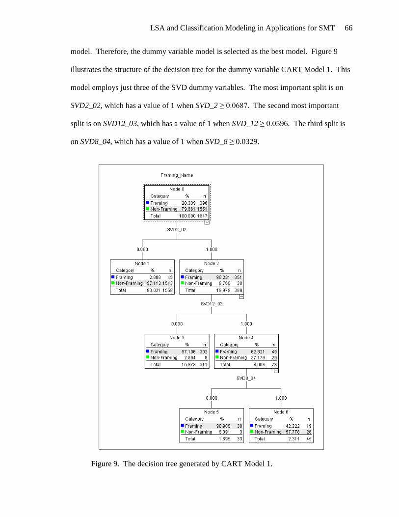
LSA and Classification Modeling in Applications for SMT 66
model. Therefore, the dummy variable model is selected as the best model. Figure 9
illustrates the structure of the decision tree for the dummy variable CART Model 1. This
model employs just three of the SVD dummy variables. The most important split is on
SVD2_02, which has a value of 1 when SVD_2 ≥ 0.0687. The second most important
split is on SVD12_03, which has a value of 1 when SVD_12 ≥ 0.0596. The third split is
on SVD8_04, which has a value of 1 when SVD_8 ≥ 0.0329.
Figure 9. The decision tree generated by CART Model 1.
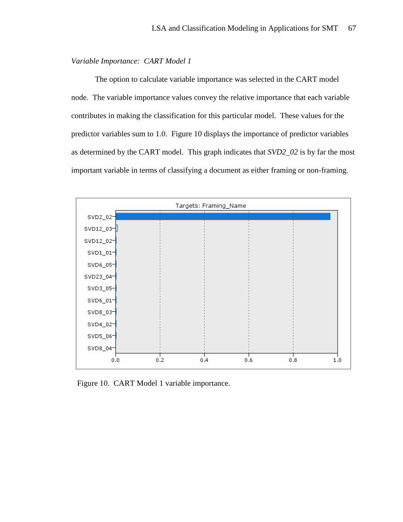
LSA and Classification Modeling in Applications for SMT 67
Variable Importance: CART Model 1
The option to calculate variable importance was selected in the CART model
node. The variable importance values convey the relative importance that each variable
contributes in making the classification for this particular model. These values for the
predictor variables sum to 1.0. Figure 10 displays the importance of predictor variables
as determined by the CART model. This graph indicates that SVD2_02 is by far the most
important variable in terms of classifying a document as either framing or non-framing.
Figure 10. CART Model 1 variable importance.
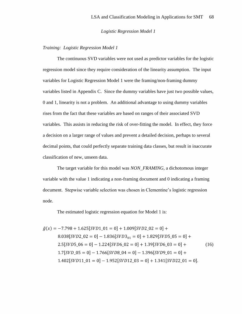
LSA and Classification Modeling in Applications for SMT 68
Logistic Regression Model 1
Training: Logistic Regression Model 1
The continuous SVD variables were not used as predictor variables for the logistic
regression model since they require consideration of the linearity assumption. The input
variables for Logistic Regression Model 1 were the framing/non-framing dummy
variables listed in Appendix C. Since the dummy variables have just two possible values,
0 and 1, linearity is not a problem. An additional advantage to using dummy variables
rises from the fact that these variables are based on ranges of their associated SVD
variables. This assists in reducing the risk of over-fitting the model. In effect, they force
a decision on a larger range of values and prevent a detailed decision, perhaps to several
decimal points, that could perfectly separate training data classes, but result in inaccurate
classification of new, unseen data.
The target variable for this model was NON_FRAMING, a dichotomous integer
variable with the value 1 indicating a non-framing document and 0 indicating a framing
document. Stepwise variable selection was chosen in Clementine‟s logistic regression
node.
The estimated logistic regression equation for Model 1 is:
(16)
.
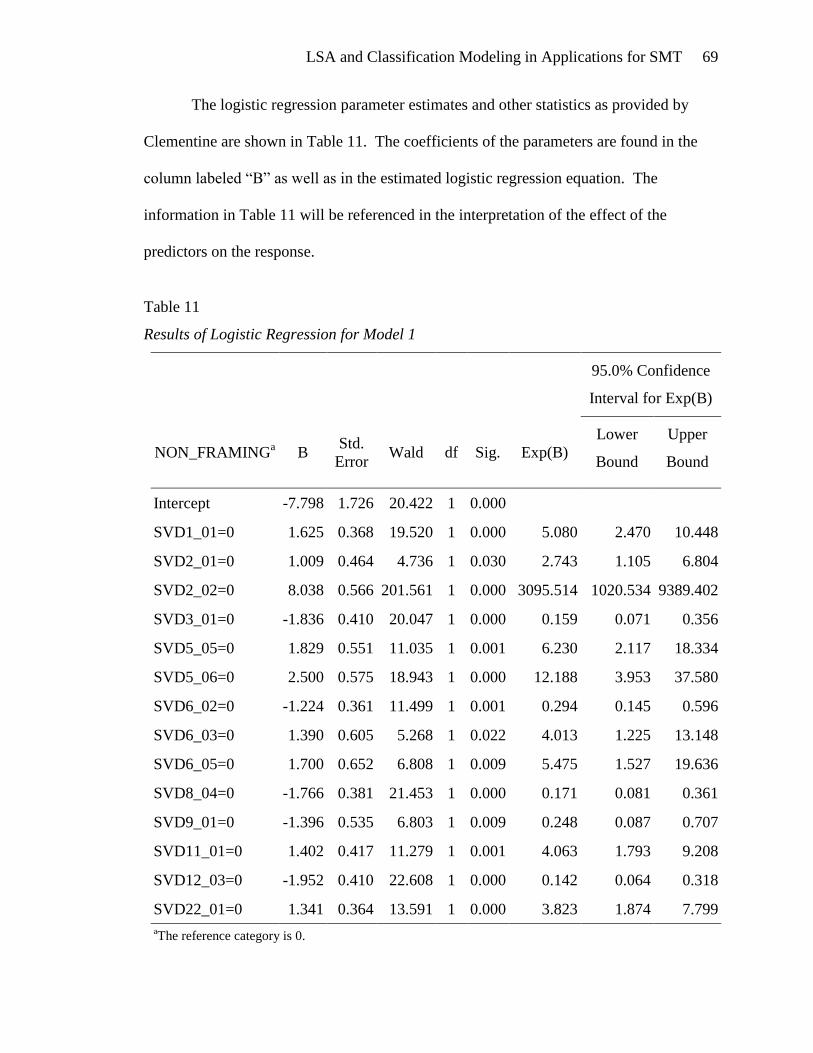
LSA and Classification Modeling in Applications for SMT 69
The logistic regression parameter estimates and other statistics as provided by
Clementine are shown in Table 11. The coefficients of the parameters are found in the
column labeled “B” as well as in the estimated logistic regression equation. The
information in Table 11 will be referenced in the interpretation of the effect of the
predictors on the response.
Table 11
Results of Logistic Regression for Model 1
95.0% Confidence
Interval for Exp(B)
NON_FRAMINGa B
Std.
Error Wald df Sig. Exp(B)
Lower
Bound
Upper
Bound
Intercept -7.798 1.726 20.422 1 0.000
SVD1_01=0 1.625 0.368 19.520 1 0.000 5.080 2.470 10.448
SVD2_01=0 1.009 0.464 4.736 1 0.030 2.743 1.105 6.804
SVD2_02=0 8.038 0.566 201.561 1 0.000 3095.514 1020.534 9389.402
SVD3_01=0 -1.836 0.410 20.047 1 0.000 0.159 0.071 0.356
SVD5_05=0 1.829 0.551 11.035 1 0.001 6.230 2.117 18.334
SVD5_06=0 2.500 0.575 18.943 1 0.000 12.188 3.953 37.580
SVD6_02=0 -1.224 0.361 11.499 1 0.001 0.294 0.145 0.596
SVD6_03=0 1.390 0.605 5.268 1 0.022 4.013 1.225 13.148
SVD6_05=0 1.700 0.652 6.808 1 0.009 5.475 1.527 19.636
SVD8_04=0 -1.766 0.381 21.453 1 0.000 0.171 0.081 0.361
SVD9_01=0 -1.396 0.535 6.803 1 0.009 0.248 0.087 0.707
SVD11_01=0 1.402 0.417 11.279 1 0.001 4.063 1.793 9.208
SVD12_03=0 -1.952 0.410 22.608 1 0.000 0.142 0.064 0.318
SVD22_01=0 1.341 0.364 13.591 1 0.000 3.823 1.874 7.799
aThe reference category is 0.
LSA and Classification Modeling in Applications for SMT 70
Effect of the Predictors on the Response
All fourteen predictor variables in Logistic Regression Model 1 have two possible
values of either 0 or 1. The odds ratios (OR) for each of these variables is in the column
labeled “Exp(B)” in Table 11 and is calculated as:
eOR (18)
The odds ratio expresses the odds that a document is non-framing when it has a
value of zero for these dichotomous predictors. An odds ratio of one means the
document is just as likely to be framing as it is to be non-framing. If it is greater than
one, the document is more likely to be non-framing. Conversely, an odds ratio that is less
than one means the document is more likely to be framing.
For example, the odds ratio of 5.080 for SVD1_01 can be interpreted as “if
SVD1_01 for a particular document is equal to zero, then that document is more than five
times more likely to be non-framing than it is to be framing.” In the case of SVD2_02,
with an odds ratio of 3095.514, one may say that “if SVD2_02 is equal to zero, then a
non-framing classification is more than 3,000 times as likely compared to a framing
classification.” Apparently, SVD2_02 is a powerful predictor of the framing status of a
document.
The Wald test for the significance of each of the parameters can be found in Table
11 under the column labeled “Wald.” This is calculated as the coefficient estimate
divided by the standard error of the coefficient. The p-value, P(|z| > Wald), for each
variable is in the column labeled “Sig.” Each of the dichotomous variables has a p-value
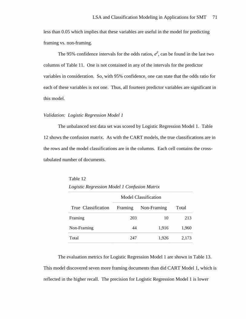
LSA and Classification Modeling in Applications for SMT 71
less than 0.05 which implies that these variables are useful in the model for predicting
framing vs. non-framing.
The 95% confidence intervals for the odds ratios, eβ, can be found in the last two
columns of Table 11. One is not contained in any of the intervals for the predictor
variables in consideration. So, with 95% confidence, one can state that the odds ratio for
each of these variables is not one. Thus, all fourteen predictor variables are significant in
this model.
Validation: Logistic Regression Model 1
The unbalanced test data set was scored by Logistic Regression Model 1. Table
12 shows the confusion matrix. As with the CART models, the true classifications are in
the rows and the model classifications are in the columns. Each cell contains the cross-
tabulated number of documents.
Table 12
Logistic Regression Model 1 Confusion Matrix
True Classification
Model Classification
Total Framing Non-Framing
Framing 203 10 213
Non-Framing 44 1,916 1,960
Total 247 1,926 2,173
The evaluation metrics for Logistic Regression Model 1 are shown in Table 13.
This model discovered seven more framing documents than did CART Model 1, which is
reflected in the higher recall. The precision for Logistic Regression Model 1 is lower
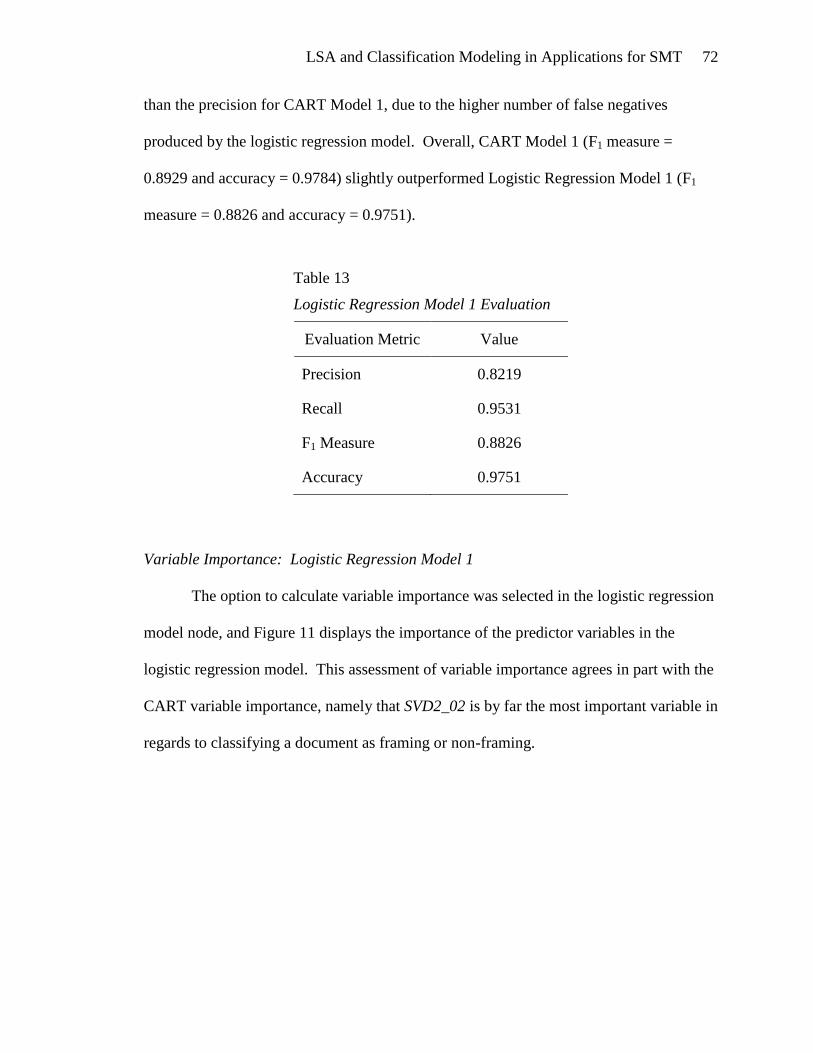
LSA and Classification Modeling in Applications for SMT 72
than the precision for CART Model 1, due to the higher number of false negatives
produced by the logistic regression model. Overall, CART Model 1 (F1 measure =
0.8929 and accuracy = 0.9784) slightly outperformed Logistic Regression Model 1 (F1
measure = 0.8826 and accuracy = 0.9751).
Table 13
Logistic Regression Model 1 Evaluation
Evaluation Metric Value
Precision 0.8219
Recall 0.9531
F1 Measure 0.8826
Accuracy 0.9751
Variable Importance: Logistic Regression Model 1
The option to calculate variable importance was selected in the logistic regression
model node, and Figure 11 displays the importance of the predictor variables in the
logistic regression model. This assessment of variable importance agrees in part with the
CART variable importance, namely that SVD2_02 is by far the most important variable in
regards to classifying a document as framing or non-framing.
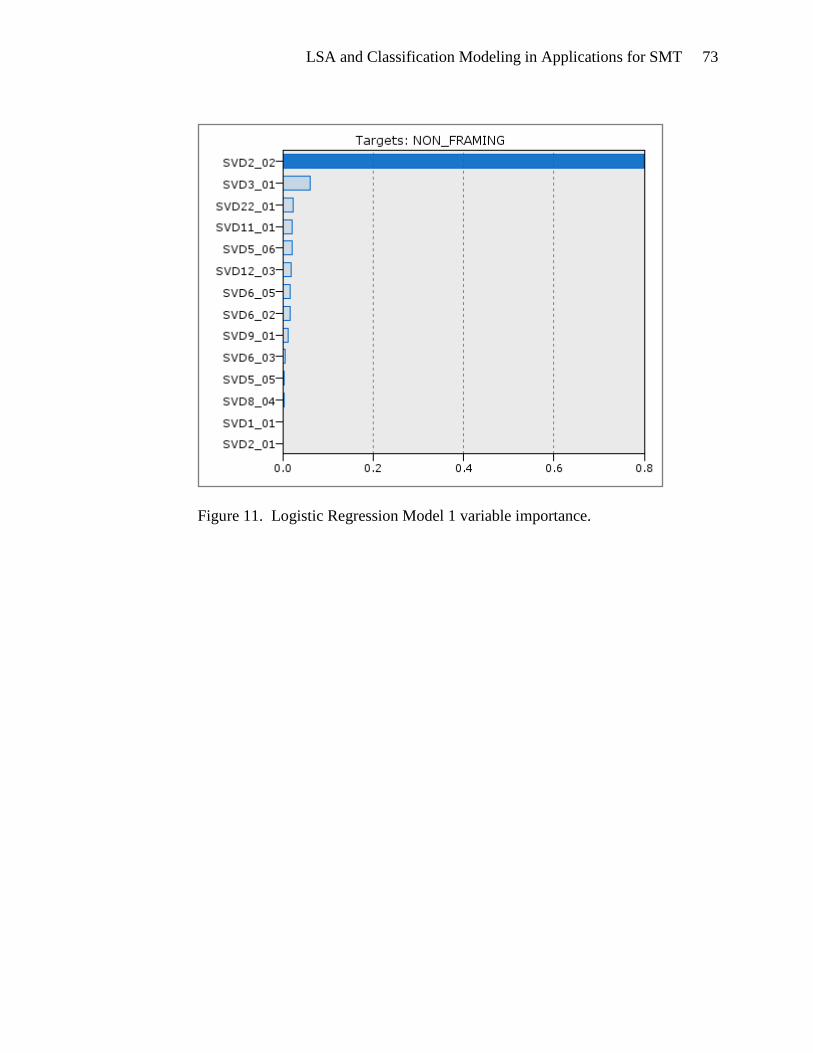
LSA and Classification Modeling in Applications for SMT 73
Figure 11. Logistic Regression Model 1 variable importance.
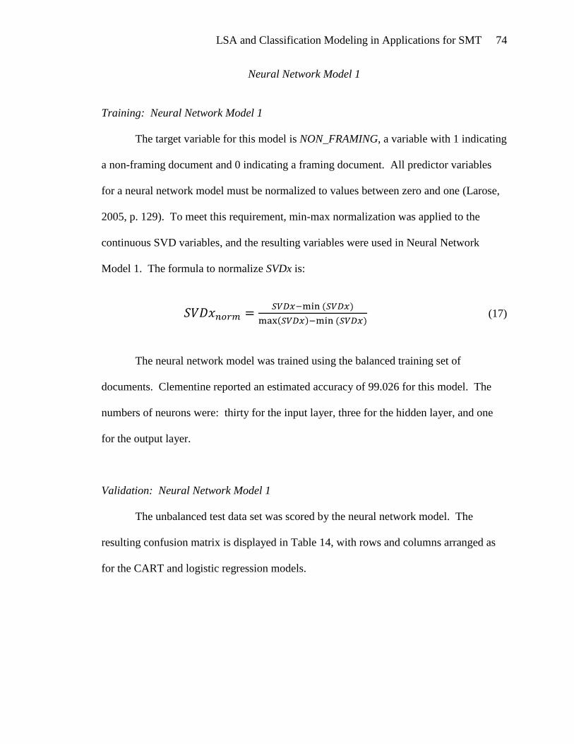
LSA and Classification Modeling in Applications for SMT 74
Neural Network Model 1
Training: Neural Network Model 1
The target variable for this model is NON_FRAMING, a variable with 1 indicating
a non-framing document and 0 indicating a framing document. All predictor variables
for a neural network model must be normalized to values between zero and one (Larose,
2005, p. 129). To meet this requirement, min-max normalization was applied to the
continuous SVD variables, and the resulting variables were used in Neural Network
Model 1. The formula to normalize SVDx is:
(17)
The neural network model was trained using the balanced training set of
documents. Clementine reported an estimated accuracy of 99.026 for this model. The
numbers of neurons were: thirty for the input layer, three for the hidden layer, and one
for the output layer.
Validation: Neural Network Model 1
The unbalanced test data set was scored by the neural network model. The
resulting confusion matrix is displayed in Table 14, with rows and columns arranged as
for the CART and logistic regression models.
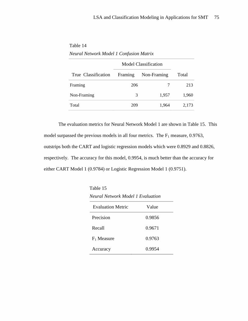
LSA and Classification Modeling in Applications for SMT 75
Table 14
Neural Network Model 1 Confusion Matrix
True Classification
Model Classification
Total Framing Non-Framing
Framing 206 7 213
Non-Framing 3 1,957 1,960
Total 209 1,964 2,173
The evaluation metrics for Neural Network Model 1 are shown in Table 15. This
model surpassed the previous models in all four metrics. The F1 measure, 0.9763,
outstrips both the CART and logistic regression models which were 0.8929 and 0.8826,
respectively. The accuracy for this model, 0.9954, is much better than the accuracy for
either CART Model 1 (0.9784) or Logistic Regression Model 1 (0.9751).
Table 15
Neural Network Model 1 Evaluation
Evaluation Metric Value
Precision 0.9856
Recall 0.9671
F1 Measure 0.9763
Accuracy 0.9954
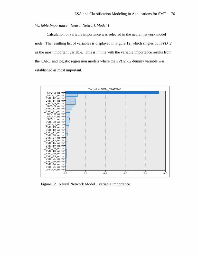
LSA and Classification Modeling in Applications for SMT 76
Variable Importance: Neural Network Model 1
Calculation of variable importance was selected in the neural network model
node. The resulting list of variables is displayed in Figure 12, which singles out SVD_2
as the most important variable. This is in line with the variable importance results from
the CART and logistic regression models where the SVD2_02 dummy variable was
established as most important.
Figure 12. Neural Network Model 1 variable importance.
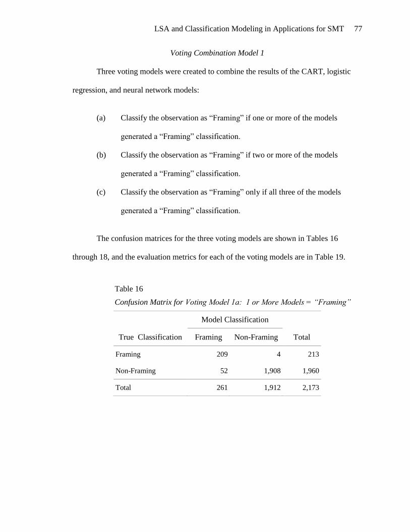
LSA and Classification Modeling in Applications for SMT 77
Voting Combination Model 1
Three voting models were created to combine the results of the CART, logistic
regression, and neural network models:
(a) Classify the observation as “Framing” if one or more of the models
generated a “Framing” classification.
(b) Classify the observation as “Framing” if two or more of the models
generated a “Framing” classification.
(c) Classify the observation as “Framing” only if all three of the models
generated a “Framing” classification.
The confusion matrices for the three voting models are shown in Tables 16
through 18, and the evaluation metrics for each of the voting models are in Table 19.
Table 16
Confusion Matrix for Voting Model 1a: 1 or More Models = “Framing”
True Classification
Model Classification
Total Framing Non-Framing
Framing 209 4 213
Non-Framing 52 1,908 1,960
Total 261 1,912 2,173
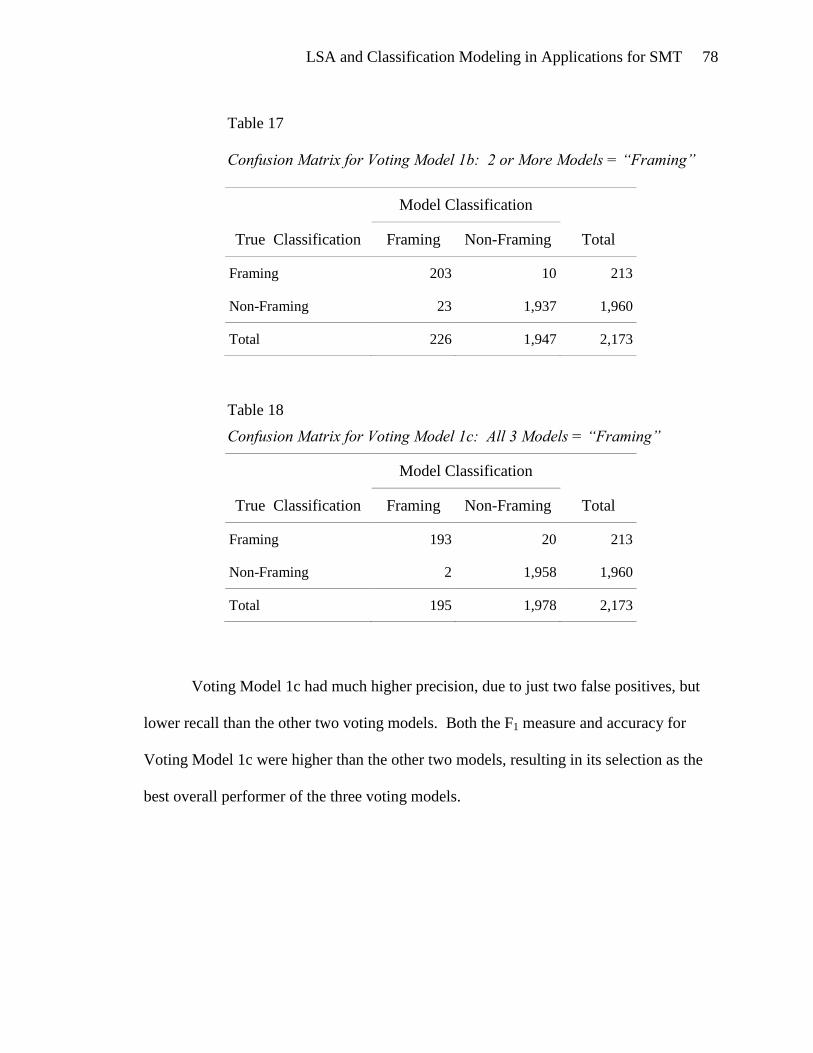
LSA and Classification Modeling in Applications for SMT 78
Table 17
Confusion Matrix for Voting Model 1b: 2 or More Models = “Framing”
True Classification
Model Classification
Total Framing Non-Framing
Framing 203 10 213
Non-Framing 23 1,937 1,960
Total 226 1,947 2,173
Table 18
Confusion Matrix for Voting Model 1c: All 3 Models = “Framing”
True Classification
Model Classification
Total Framing Non-Framing
Framing 193 20 213
Non-Framing 2 1,958 1,960
Total 195 1,978 2,173
Voting Model 1c had much higher precision, due to just two false positives, but
lower recall than the other two voting models. Both the F1 measure and accuracy for
Voting Model 1c were higher than the other two models, resulting in its selection as the
best overall performer of the three voting models.
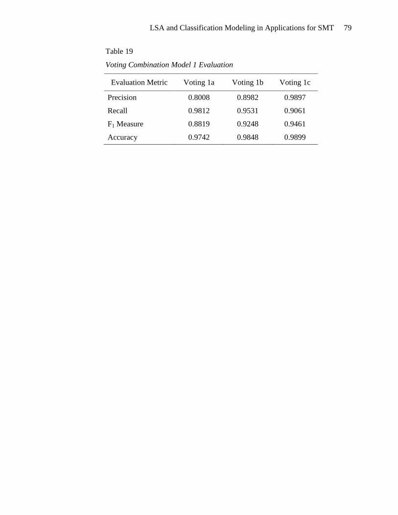
LSA and Classification Modeling in Applications for SMT 79
Table 19
Voting Combination Model 1 Evaluation
Evaluation Metric Voting 1a Voting 1b Voting 1c
Precision 0.8008 0.8982 0.9897
Recall 0.9812 0.9531 0.9061
F1 Measure 0.8819 0.9248 0.9461
Accuracy 0.9742 0.9848 0.9899
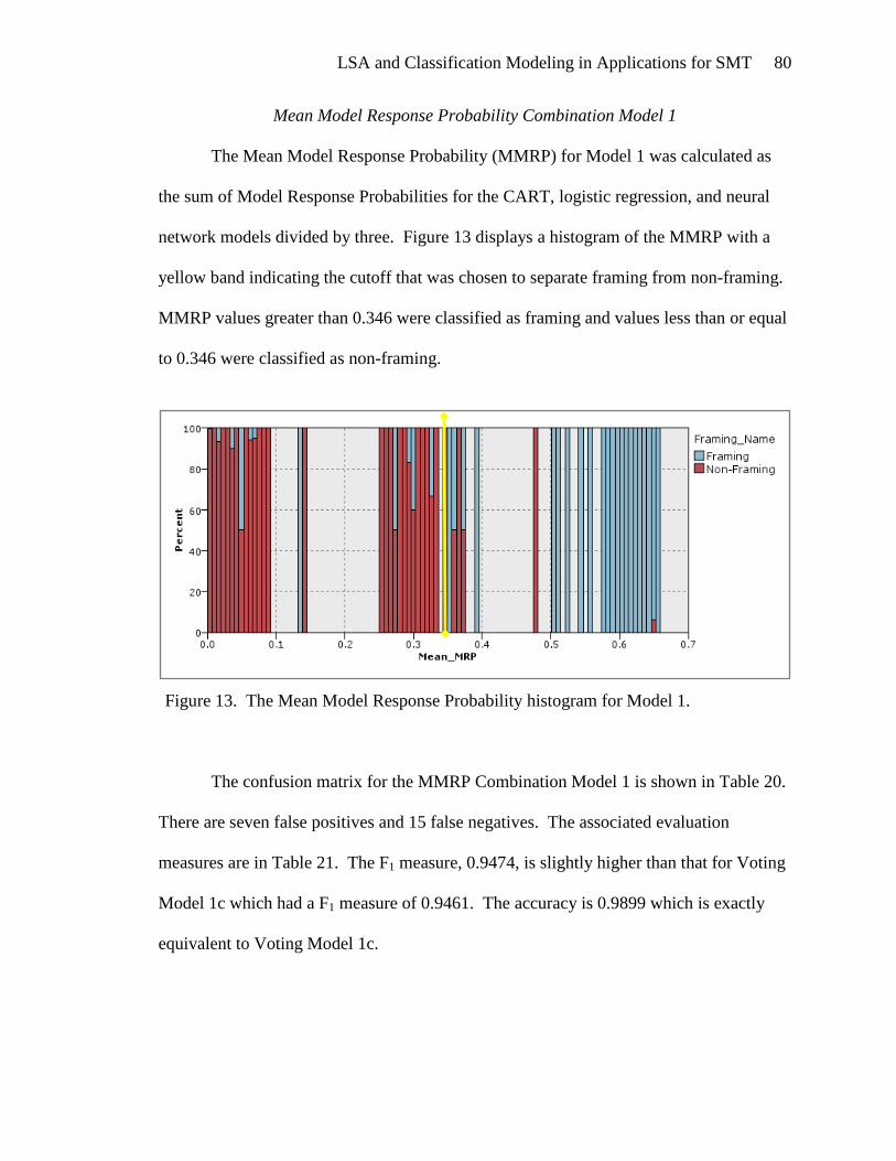
LSA and Classification Modeling in Applications for SMT 80
Mean Model Response Probability Combination Model 1
The Mean Model Response Probability (MMRP) for Model 1 was calculated as
the sum of Model Response Probabilities for the CART, logistic regression, and neural
network models divided by three. Figure 13 displays a histogram of the MMRP with a
yellow band indicating the cutoff that was chosen to separate framing from non-framing.
MMRP values greater than 0.346 were classified as framing and values less than or equal
to 0.346 were classified as non-framing.
Figure 13. The Mean Model Response Probability histogram for Model 1.
The confusion matrix for the MMRP Combination Model 1 is shown in Table 20.
There are seven false positives and 15 false negatives. The associated evaluation
measures are in Table 21. The F1 measure, 0.9474, is slightly higher than that for Voting
Model 1c which had a F1 measure of 0.9461. The accuracy is 0.9899 which is exactly
equivalent to Voting Model 1c.
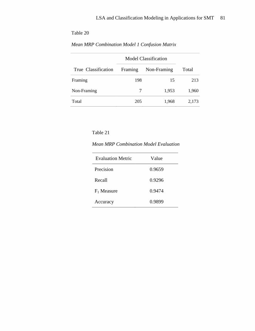
LSA and Classification Modeling in Applications for SMT 81
Table 20
Mean MRP Combination Model 1 Confusion Matrix
True Classification
Model Classification
Total Framing Non-Framing
Framing 198 15 213
Non-Framing 7 1,953 1,960
Total 205 1,968 2,173
Table 21
Mean MRP Combination Model Evaluation
Evaluation Metric Value
Precision 0.9659
Recall 0.9296
F1 Measure 0.9474
Accuracy 0.9899
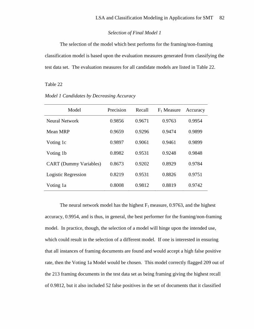
LSA and Classification Modeling in Applications for SMT 82
Selection of Final Model 1
The selection of the model which best performs for the framing/non-framing
classification model is based upon the evaluation measures generated from classifying the
test data set. The evaluation measures for all candidate models are listed in Table 22.
Table 22
Model 1 Candidates by Decreasing Accuracy
Model Precision Recall F1 Measure Accuracy
Neural Network 0.9856 0.9671 0.9763 0.9954
Mean MRP 0.9659 0.9296 0.9474 0.9899
Voting 1c 0.9897 0.9061 0.9461 0.9899
Voting 1b 0.8982 0.9531 0.9248 0.9848
CART (Dummy Variables) 0.8673 0.9202 0.8929 0.9784
Logistic Regression 0.8219 0.9531 0.8826 0.9751
Voting 1a 0.8008 0.9812 0.8819 0.9742
The neural network model has the highest F1 measure, 0.9763, and the highest
accuracy, 0.9954, and is thus, in general, the best performer for the framing/non-framing
model. In practice, though, the selection of a model will hinge upon the intended use,
which could result in the selection of a different model. If one is interested in ensuring
that all instances of framing documents are found and would accept a high false positive
rate, then the Voting 1a Model would be chosen. This model correctly flagged 209 out of
the 213 framing documents in the test data set as being framing giving the highest recall
of 0.9812, but it also included 52 false positives in the set of documents that it classified

LSA and Classification Modeling in Applications for SMT 83
as framing, resulting in the lowest precision, 0.8008. If one requires high precision in
correctly identifying framing documents, then the Voting 1c Model would be chosen.
This model classified 195 documents as framing and only two of those documents were
in reality non-framing, giving a precision of 0.9897.
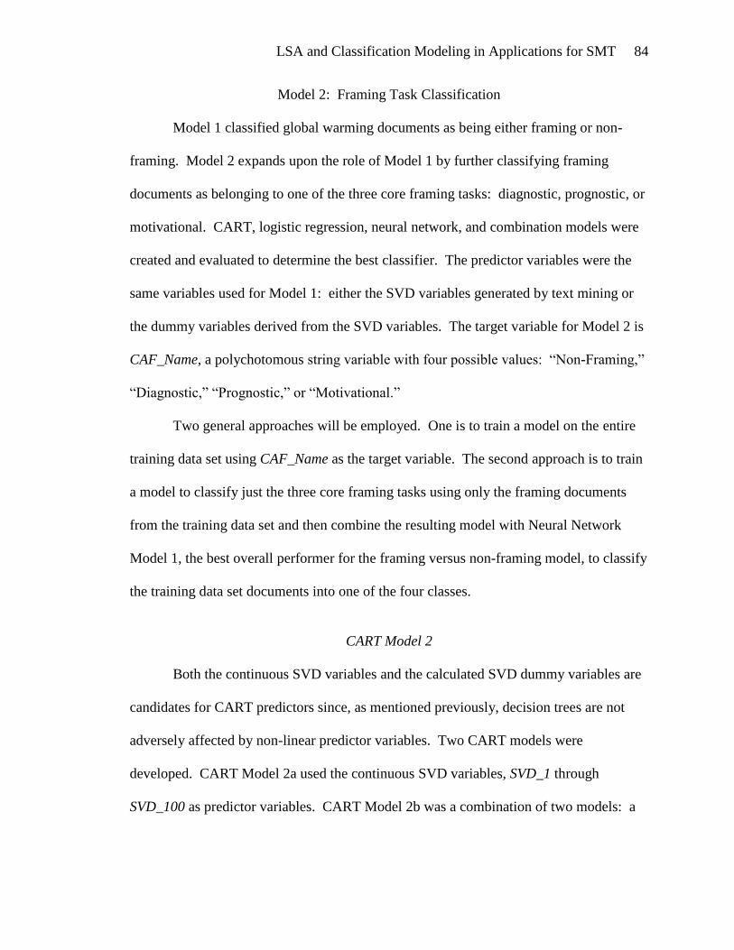
LSA and Classification Modeling in Applications for SMT 84
Model 2: Framing Task Classification
Model 1 classified global warming documents as being either framing or non-
framing. Model 2 expands upon the role of Model 1 by further classifying framing
documents as belonging to one of the three core framing tasks: diagnostic, prognostic, or
motivational. CART, logistic regression, neural network, and combination models were
created and evaluated to determine the best classifier. The predictor variables were the
same variables used for Model 1: either the SVD variables generated by text mining or
the dummy variables derived from the SVD variables. The target variable for Model 2 is
CAF_Name, a polychotomous string variable with four possible values: “Non-Framing,”
“Diagnostic,” “Prognostic,” or “Motivational.”
Two general approaches will be employed. One is to train a model on the entire
training data set using CAF_Name as the target variable. The second approach is to train
a model to classify just the three core framing tasks using only the framing documents
from the training data set and then combine the resulting model with Neural Network
Model 1, the best overall performer for the framing versus non-framing model, to classify
the training data set documents into one of the four classes.
CART Model 2
Both the continuous SVD variables and the calculated SVD dummy variables are
candidates for CART predictors since, as mentioned previously, decision trees are not
adversely affected by non-linear predictor variables. Two CART models were
developed. CART Model 2a used the continuous SVD variables, SVD_1 through
SVD_100 as predictor variables. CART Model 2b was a combination of two models: a
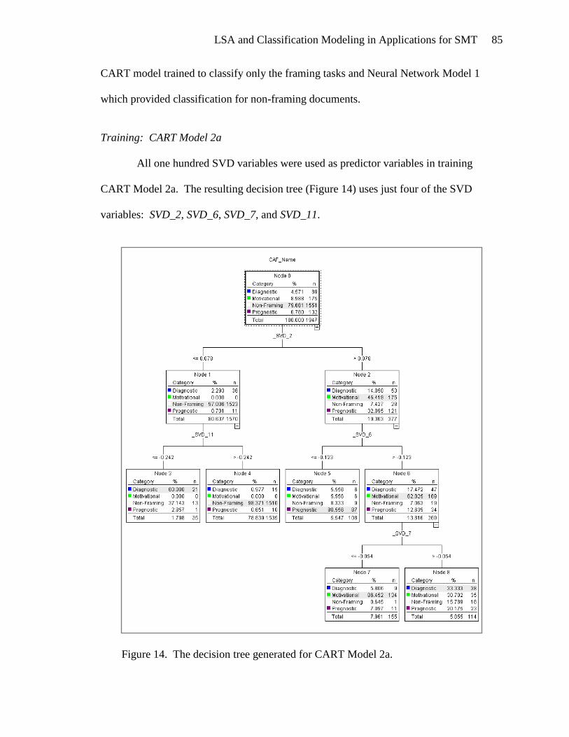
LSA and Classification Modeling in Applications for SMT 85
CART model trained to classify only the framing tasks and Neural Network Model 1
which provided classification for non-framing documents.
Training: CART Model 2a
All one hundred SVD variables were used as predictor variables in training
CART Model 2a. The resulting decision tree (Figure 14) uses just four of the SVD
variables: SVD_2, SVD_6, SVD_7, and SVD_11.
Figure 14. The decision tree generated for CART Model 2a.
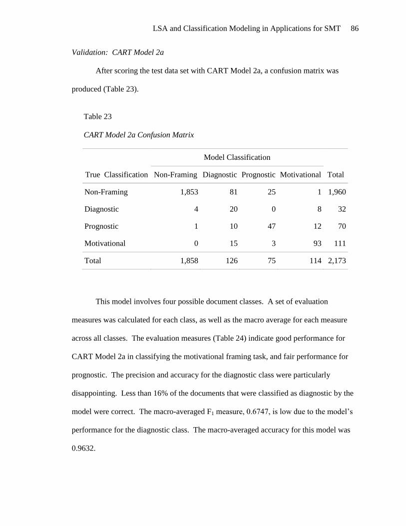
LSA and Classification Modeling in Applications for SMT 86
Validation: CART Model 2a
After scoring the test data set with CART Model 2a, a confusion matrix was
produced (Table 23).
Table 23
CART Model 2a Confusion Matrix
True Classification
Model Classification
Total Non-Framing Diagnostic Prognostic Motivational
Non-Framing 1,853 81 25 1 1,960
Diagnostic 4 20 0 8 32
Prognostic 1 10 47 12 70
Motivational 0 15 3 93 111
Total 1,858 126 75 114 2,173
This model involves four possible document classes. A set of evaluation
measures was calculated for each class, as well as the macro average for each measure
across all classes. The evaluation measures (Table 24) indicate good performance for
CART Model 2a in classifying the motivational framing task, and fair performance for
prognostic. The precision and accuracy for the diagnostic class were particularly
disappointing. Less than 16% of the documents that were classified as diagnostic by the
model were correct. The macro-averaged F1 measure, 0.6747, is low due to the model‟s
performance for the diagnostic class. The macro-averaged accuracy for this model was
0.9632.
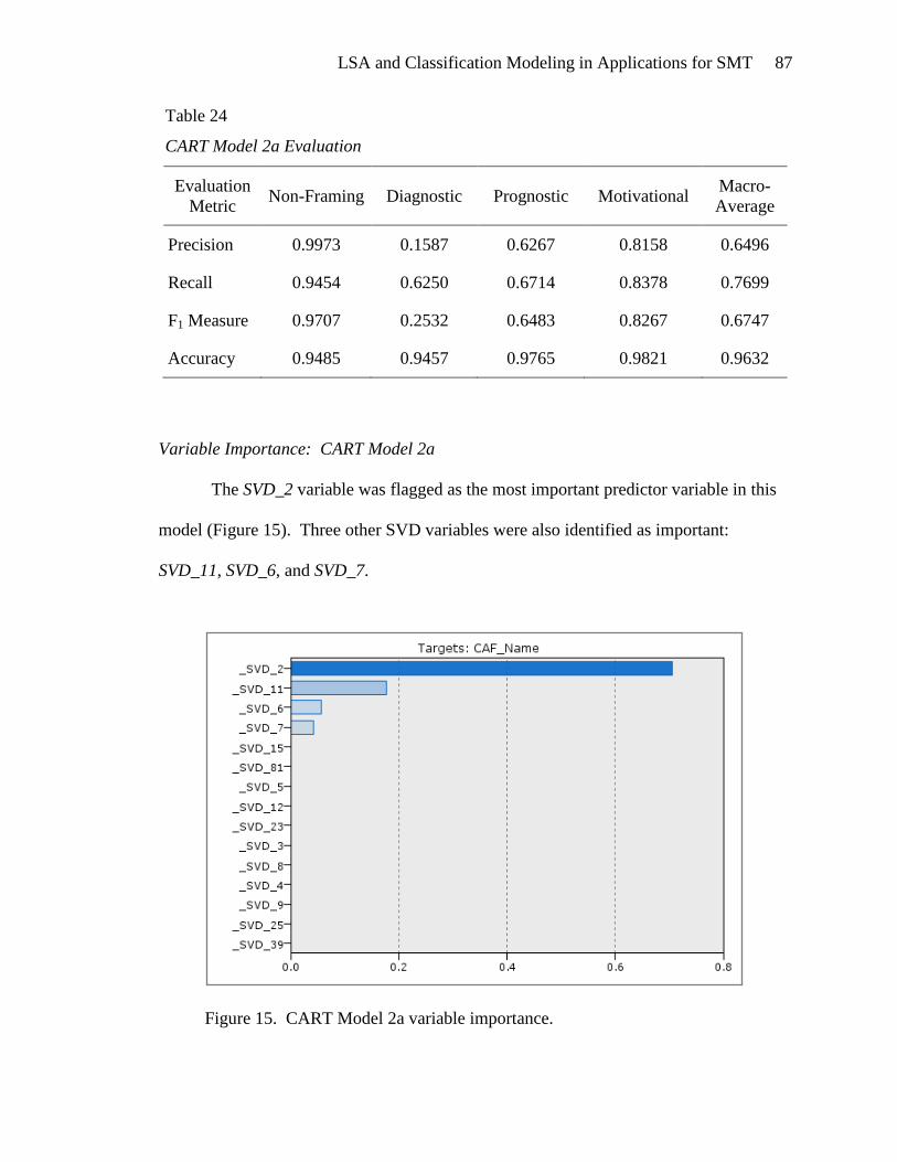
LSA and Classification Modeling in Applications for SMT 87
Table 24
CART Model 2a Evaluation
Evaluation
Metric Non-Framing Diagnostic Prognostic Motivational
Macro-
Average
Precision 0.9973 0.1587 0.6267 0.8158 0.6496
Recall 0.9454 0.6250 0.6714 0.8378 0.7699
F1 Measure 0.9707 0.2532 0.6483 0.8267 0.6747
Accuracy 0.9485 0.9457 0.9765 0.9821 0.9632
Variable Importance: CART Model 2a
The SVD_2 variable was flagged as the most important predictor variable in this
model (Figure 15). Three other SVD variables were also identified as important:
SVD_11, SVD_6, and SVD_7.
Figure 15. CART Model 2a variable importance.

LSA and Classification Modeling in Applications for SMT 88
CART Model 2b
CART Model 2b is a combination of a CART model that classifies the framing
documents by core task and Neural Network Model 1 that classifies documents by
framing vs. non-framing. The first step is the development of the CART model for
Diagnostic/Prognostic/Motivational (DPM) classification. There are two possible sets of
predictor variables for this model: the continuous SVD variables and the SVD DPM
dummy variables (Appendix D). Two CART models were developed, one for each set of
predictor variables. These models are labeled CART DPM SVD, using continuous SVD
variables, and CART DPM DV, using dummy predictor variables. The models were
trained using only the framing documents from the training data set.
The framing documents from the test data set were scored with each CART DPM
model. The resultant confusion matrices are shown in Table 25 (CART DPM SVD) and
Table 26 (CART DPM DV).
Table 25
CART DPM SVD Confusion Matrix
True Classification
Model Classification Total
Diagnostic Prognostic Motivational
Diagnostic 20 3 9 32
Prognostic 7 50 13 70
Motivational 7 5 99 111
Total 34 58 121 213
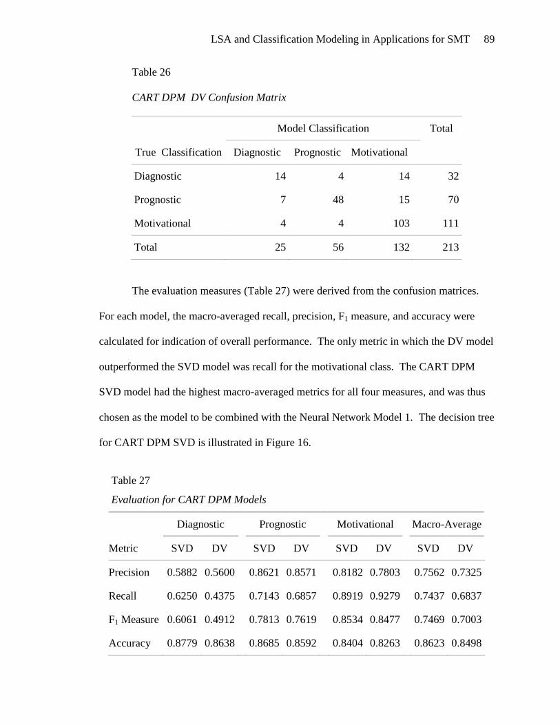
LSA and Classification Modeling in Applications for SMT 89
Table 26
CART DPM DV Confusion Matrix
True Classification
Model Classification Total
Diagnostic Prognostic Motivational
Diagnostic 14 4 14 32
Prognostic 7 48 15 70
Motivational 4 4 103 111
Total 25 56 132 213
The evaluation measures (Table 27) were derived from the confusion matrices.
For each model, the macro-averaged recall, precision, F1 measure, and accuracy were
calculated for indication of overall performance. The only metric in which the DV model
outperformed the SVD model was recall for the motivational class. The CART DPM
SVD model had the highest macro-averaged metrics for all four measures, and was thus
chosen as the model to be combined with the Neural Network Model 1. The decision tree
for CART DPM SVD is illustrated in Figure 16.
Table 27
Evaluation for CART DPM Models
Diagnostic Prognostic Motivational Macro-Average
Metric SVD DV SVD DV SVD DV SVD DV
Precision 0.5882 0.5600 0.8621 0.8571 0.8182 0.7803 0.7562 0.7325
Recall 0.6250 0.4375 0.7143 0.6857 0.8919 0.9279 0.7437 0.6837
F1 Measure 0.6061 0.4912 0.7813 0.7619 0.8534 0.8477 0.7469 0.7003
Accuracy 0.8779 0.8638 0.8685 0.8592 0.8404 0.8263 0.8623 0.8498
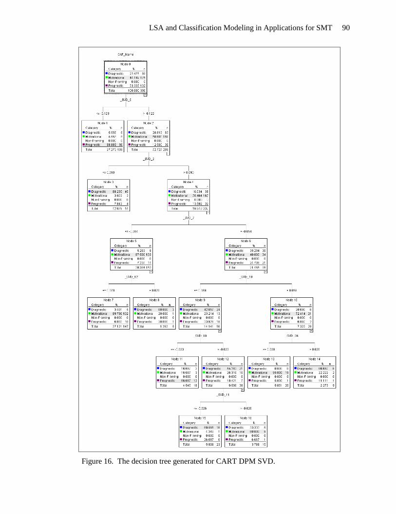
LSA and Classification Modeling in Applications for SMT 90
Figure 16. The decision tree generated for CART DPM SVD.
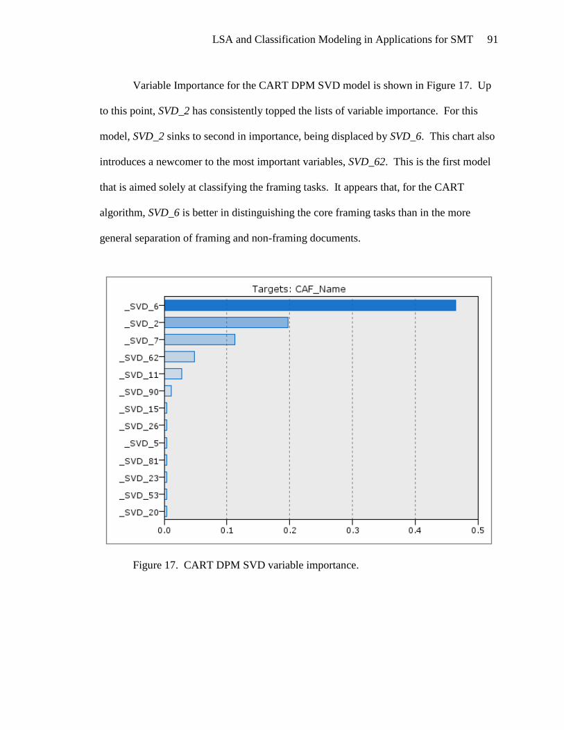
LSA and Classification Modeling in Applications for SMT 91
Variable Importance for the CART DPM SVD model is shown in Figure 17. Up
to this point, SVD_2 has consistently topped the lists of variable importance. For this
model, SVD_2 sinks to second in importance, being displaced by SVD_6. This chart also
introduces a newcomer to the most important variables, SVD_62. This is the first model
that is aimed solely at classifying the framing tasks. It appears that, for the CART
algorithm, SVD_6 is better in distinguishing the core framing tasks than in the more
general separation of framing and non-framing documents.
Figure 17. CART DPM SVD variable importance.
LSA and Classification Modeling in Applications for SMT 92
The CART DPM SVD model was combined with Neural Network Model 1 to
create a new model, CART Model 2b, that can identify all four classes: non-framing,
diagnostic, prognostic, and motivational. The final classification was determined by the
following logic:
if CART_DPM_SVD_conf >= NN_NF_conf then
CART_DPM_SVD
elseif NN_NF = “Framing” then
CART_DPM_SVD
else
"Non-Framing"
endif
In essence, if the CART DPM SVD model has higher confidence in its decision
than Neural Network Model 1, then the observation is classified according to the CART
DPM SVD model. This means the observation is a framing document and is identified as
one of the core framing tasks. If Neural Network Model 1 has the higher confidence and
classified the observation as “Framing,” then the CART DPM SVD model‟s
classification is used to provide classification by framing task. Finally, if Neural
Network Model 1 has a higher confidence and has classified the observation as “Non-
Framing,” then that will be the final classification for the observation.
In addition to determining the classification of the combined model, the
associated confidence is also assigned to the decision. If the observation was classified
as “Non-Framing,” then the combined model confidence is set to the confidence of
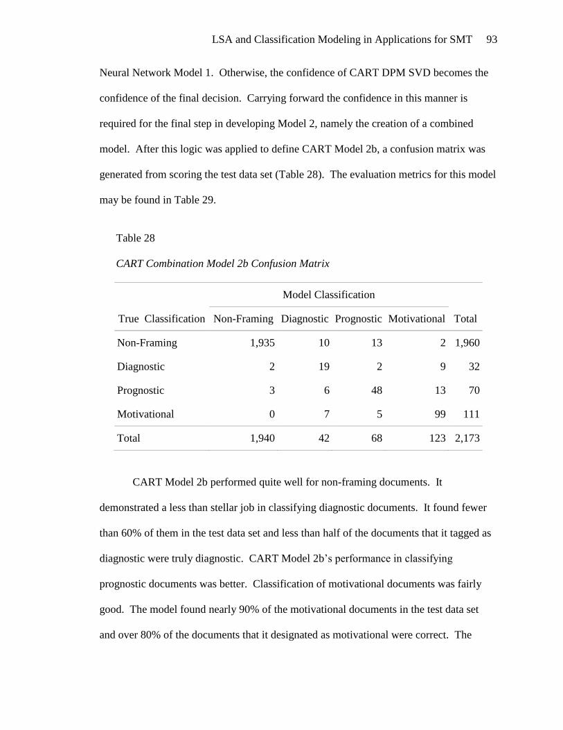
LSA and Classification Modeling in Applications for SMT 93
Neural Network Model 1. Otherwise, the confidence of CART DPM SVD becomes the
confidence of the final decision. Carrying forward the confidence in this manner is
required for the final step in developing Model 2, namely the creation of a combined
model. After this logic was applied to define CART Model 2b, a confusion matrix was
generated from scoring the test data set (Table 28). The evaluation metrics for this model
may be found in Table 29.
Table 28
CART Combination Model 2b Confusion Matrix
True Classification
Model Classification
Total Non-Framing Diagnostic Prognostic Motivational
Non-Framing 1,935 10 13 2 1,960
Diagnostic 2 19 2 9 32
Prognostic 3 6 48 13 70
Motivational 0 7 5 99 111
Total 1,940 42 68 123 2,173
CART Model 2b performed quite well for non-framing documents. It
demonstrated a less than stellar job in classifying diagnostic documents. It found fewer
than 60% of them in the test data set and less than half of the documents that it tagged as
diagnostic were truly diagnostic. CART Model 2b‟s performance in classifying
prognostic documents was better. Classification of motivational documents was fairly
good. The model found nearly 90% of the motivational documents in the test data set
and over 80% of the documents that it designated as motivational were correct. The
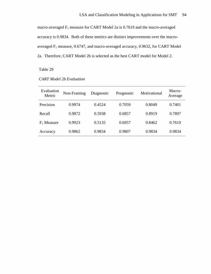
LSA and Classification Modeling in Applications for SMT 94
macro-averaged F1 measure for CART Model 2a is 0.7619 and the macro-averaged
accuracy is 0.9834. Both of these metrics are distinct improvements over the macro-
averaged F1 measure, 0.6747, and macro-averaged accuracy, 0.9632, for CART Model
2a. Therefore, CART Model 2b is selected as the best CART model for Model 2.
Table 29
CART Model 2b Evaluation
Evaluation
Metric Non-Framing Diagnostic Prognostic Motivational
Macro-
Average
Precision 0.9974 0.4524 0.7059 0.8049 0.7401
Recall 0.9872 0.5938 0.6857 0.8919 0.7897
F1 Measure 0.9923 0.5135 0.6957 0.8462 0.7619
Accuracy 0.9862 0.9834 0.9807 0.9834 0.9834
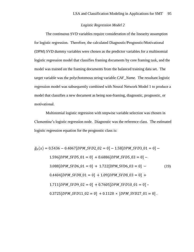
LSA and Classification Modeling in Applications for SMT 95
Logistic Regression Model 2
The continuous SVD variables require consideration of the linearity assumption
for logistic regression. Therefore, the calculated Diagnostic/Prognostic/Motivational
(DPM) SVD dummy variables were chosen as the predictor variables for a multinomial
logistic regression model that classifies framing documents by core framing task, and the
model was trained on the framing documents from the balanced training data set. The
target variable was the polychotomous string variable CAF_Name. The resultant logistic
regression model was subsequently combined with Neural Network Model 1 to produce a
model that classifies a new document as being non-framing, diagnostic, prognostic, or
motivational.
Multinomial logistic regression with stepwise variable selection was chosen in
Clementine‟s logistic regression node. Diagnostic was the reference class. The estimated
logistic regression equation for the prognostic class is:
(19)
–
.
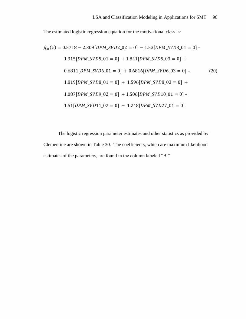
LSA and Classification Modeling in Applications for SMT 96
The estimated logistic regression equation for the motivational class is:
–
– (20)
–
.
The logistic regression parameter estimates and other statistics as provided by
Clementine are shown in Table 30. The coefficients, which are maximum likelihood
estimates of the parameters, are found in the column labeled “B.”
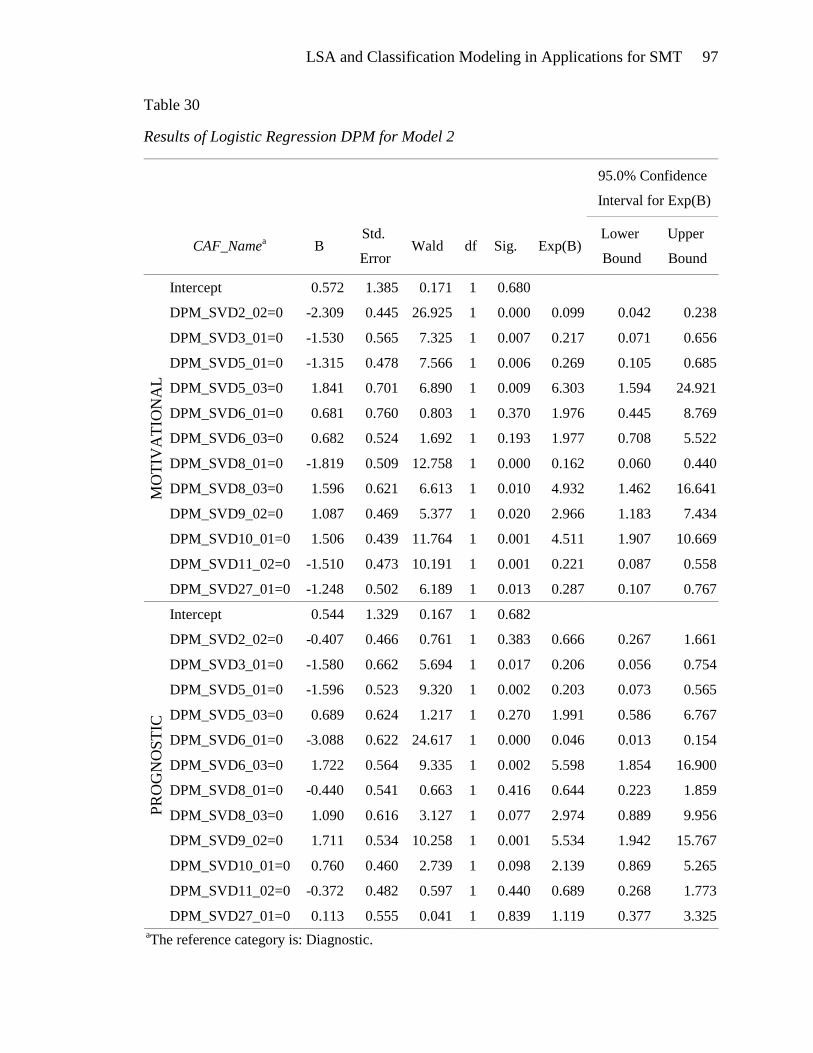
LSA and Classification Modeling in Applications for SMT 97
Table 30
Results of Logistic Regression DPM for Model 2
95.0% Confidence
Interval for Exp(B)
CAF_Namea B
Std.
Error Wald df Sig. Exp(B)
Lower
Bound
Upper
Bound
MO
TIV
AT
ION
AL
Intercept 0.572 1.385 0.171 1 0.680
DPM_SVD2_02=0 -2.309 0.445 26.925 1 0.000 0.099 0.042 0.238
DPM_SVD3_01=0 -1.530 0.565 7.325 1 0.007 0.217 0.071 0.656
DPM_SVD5_01=0 -1.315 0.478 7.566 1 0.006 0.269 0.105 0.685
DPM_SVD5_03=0 1.841 0.701 6.890 1 0.009 6.303 1.594 24.921
DPM_SVD6_01=0 0.681 0.760 0.803 1 0.370 1.976 0.445 8.769
DPM_SVD6_03=0 0.682 0.524 1.692 1 0.193 1.977 0.708 5.522
DPM_SVD8_01=0 -1.819 0.509 12.758 1 0.000 0.162 0.060 0.440
DPM_SVD8_03=0 1.596 0.621 6.613 1 0.010 4.932 1.462 16.641
DPM_SVD9_02=0 1.087 0.469 5.377 1 0.020 2.966 1.183 7.434
DPM_SVD10_01=0 1.506 0.439 11.764 1 0.001 4.511 1.907 10.669
DPM_SVD11_02=0 -1.510 0.473 10.191 1 0.001 0.221 0.087 0.558
DPM_SVD27_01=0 -1.248 0.502 6.189 1 0.013 0.287 0.107 0.767
PR
OG
NO
ST
IC
Intercept 0.544 1.329 0.167 1 0.682
DPM_SVD2_02=0 -0.407 0.466 0.761 1 0.383 0.666 0.267 1.661
DPM_SVD3_01=0 -1.580 0.662 5.694 1 0.017 0.206 0.056 0.754
DPM_SVD5_01=0 -1.596 0.523 9.320 1 0.002 0.203 0.073 0.565
DPM_SVD5_03=0 0.689 0.624 1.217 1 0.270 1.991 0.586 6.767
DPM_SVD6_01=0 -3.088 0.622 24.617 1 0.000 0.046 0.013 0.154
DPM_SVD6_03=0 1.722 0.564 9.335 1 0.002 5.598 1.854 16.900
DPM_SVD8_01=0 -0.440 0.541 0.663 1 0.416 0.644 0.223 1.859
DPM_SVD8_03=0 1.090 0.616 3.127 1 0.077 2.974 0.889 9.956
DPM_SVD9_02=0 1.711 0.534 10.258 1 0.001 5.534 1.942 15.767
DPM_SVD10_01=0 0.760 0.460 2.739 1 0.098 2.139 0.869 5.265
DPM_SVD11_02=0 -0.372 0.482 0.597 1 0.440 0.689 0.268 1.773
DPM_SVD27_01=0 0.113 0.555 0.041 1 0.839 1.119 0.377 3.325
aThe reference category is: Diagnostic.
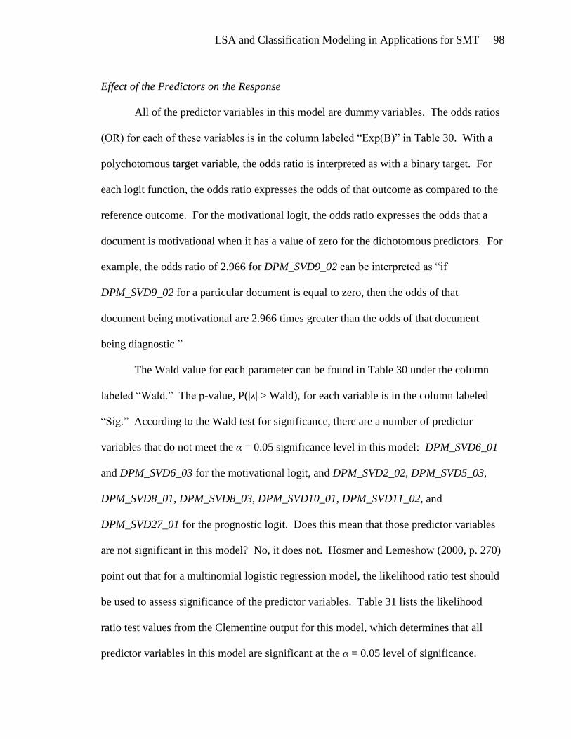
LSA and Classification Modeling in Applications for SMT 98
Effect of the Predictors on the Response
All of the predictor variables in this model are dummy variables. The odds ratios
(OR) for each of these variables is in the column labeled “Exp(B)” in Table 30. With a
polychotomous target variable, the odds ratio is interpreted as with a binary target. For
each logit function, the odds ratio expresses the odds of that outcome as compared to the
reference outcome. For the motivational logit, the odds ratio expresses the odds that a
document is motivational when it has a value of zero for the dichotomous predictors. For
example, the odds ratio of 2.966 for DPM_SVD9_02 can be interpreted as “if
DPM_SVD9_02 for a particular document is equal to zero, then the odds of that
document being motivational are 2.966 times greater than the odds of that document
being diagnostic.”
The Wald value for each parameter can be found in Table 30 under the column
labeled “Wald.” The p-value, P(|z| > Wald), for each variable is in the column labeled
“Sig.” According to the Wald test for significance, there are a number of predictor
variables that do not meet the α = 0.05 significance level in this model: DPM_SVD6_01
and DPM_SVD6_03 for the motivational logit, and DPM_SVD2_02, DPM_SVD5_03,
DPM_SVD8_01, DPM_SVD8_03, DPM_SVD10_01, DPM_SVD11_02, and
DPM_SVD27_01 for the prognostic logit. Does this mean that those predictor variables
are not significant in this model? No, it does not. Hosmer and Lemeshow (2000, p. 270)
point out that for a multinomial logistic regression model, the likelihood ratio test should
be used to assess significance of the predictor variables. Table 31 lists the likelihood
ratio test values from the Clementine output for this model, which determines that all
predictor variables in this model are significant at the α = 0.05 level of significance.
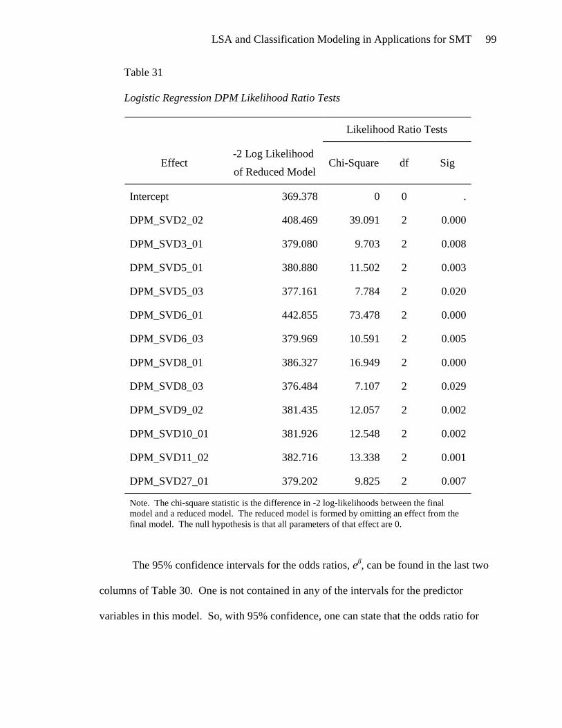
LSA and Classification Modeling in Applications for SMT 99
Table 31
Logistic Regression DPM Likelihood Ratio Tests
Likelihood Ratio Tests
Effect -2 Log Likelihood
of Reduced Model Chi-Square df Sig
Intercept 369.378 0 0 .
DPM_SVD2_02 408.469 39.091 2 0.000
DPM_SVD3_01 379.080 9.703 2 0.008
DPM_SVD5_01 380.880 11.502 2 0.003
DPM_SVD5_03 377.161 7.784 2 0.020
DPM_SVD6_01 442.855 73.478 2 0.000
DPM_SVD6_03 379.969 10.591 2 0.005
DPM_SVD8_01 386.327 16.949 2 0.000
DPM_SVD8_03 376.484 7.107 2 0.029
DPM_SVD9_02 381.435 12.057 2 0.002
DPM_SVD10_01 381.926 12.548 2 0.002
DPM_SVD11_02 382.716 13.338 2 0.001
DPM_SVD27_01 379.202 9.825 2 0.007
Note. The chi-square statistic is the difference in -2 log-likelihoods between the final
model and a reduced model. The reduced model is formed by omitting an effect from the
final model. The null hypothesis is that all parameters of that effect are 0.
The 95% confidence intervals for the odds ratios, eβ, can be found in the last two
columns of Table 30. One is not contained in any of the intervals for the predictor
variables in this model. So, with 95% confidence, one can state that the odds ratio for
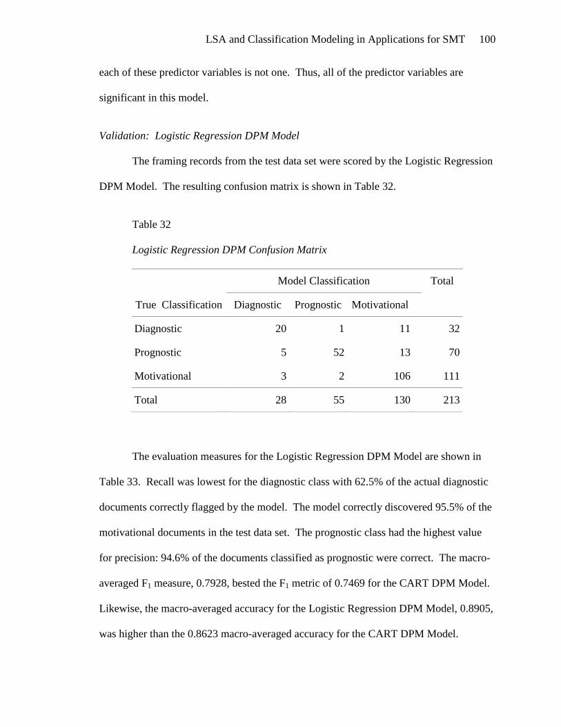
LSA and Classification Modeling in Applications for SMT 100
each of these predictor variables is not one. Thus, all of the predictor variables are
significant in this model.
Validation: Logistic Regression DPM Model
The framing records from the test data set were scored by the Logistic Regression
DPM Model. The resulting confusion matrix is shown in Table 32.
Table 32
Logistic Regression DPM Confusion Matrix
True Classification
Model Classification Total
Diagnostic Prognostic Motivational
Diagnostic 20 1 11 32
Prognostic 5 52 13 70
Motivational 3 2 106 111
Total 28 55 130 213
The evaluation measures for the Logistic Regression DPM Model are shown in
Table 33. Recall was lowest for the diagnostic class with 62.5% of the actual diagnostic
documents correctly flagged by the model. The model correctly discovered 95.5% of the
motivational documents in the test data set. The prognostic class had the highest value
for precision: 94.6% of the documents classified as prognostic were correct. The macro-
averaged F1 measure, 0.7928, bested the F1 metric of 0.7469 for the CART DPM Model.
Likewise, the macro-averaged accuracy for the Logistic Regression DPM Model, 0.8905,
was higher than the 0.8623 macro-averaged accuracy for the CART DPM Model.
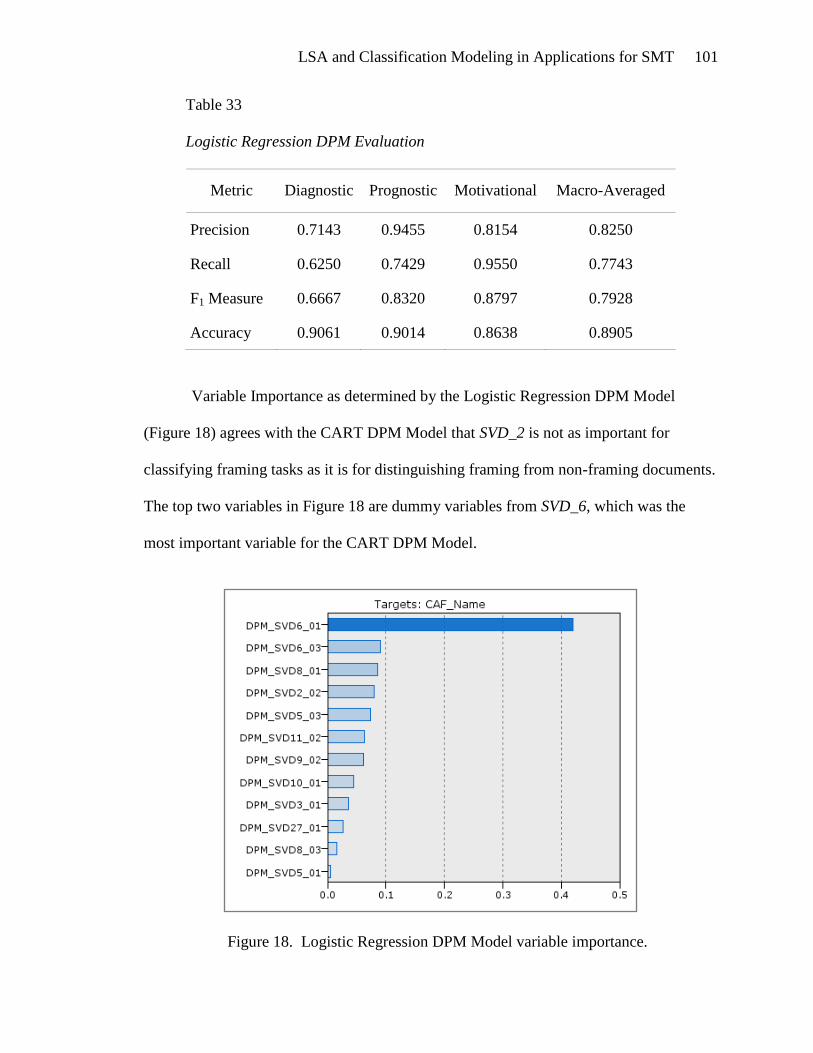
LSA and Classification Modeling in Applications for SMT 101
Table 33
Logistic Regression DPM Evaluation
Metric Diagnostic Prognostic Motivational Macro-Averaged
Precision 0.7143 0.9455 0.8154 0.8250
Recall 0.6250 0.7429 0.9550 0.7743
F1 Measure 0.6667 0.8320 0.8797 0.7928
Accuracy 0.9061 0.9014 0.8638 0.8905
Variable Importance as determined by the Logistic Regression DPM Model
(Figure 18) agrees with the CART DPM Model that SVD_2 is not as important for
classifying framing tasks as it is for distinguishing framing from non-framing documents.
The top two variables in Figure 18 are dummy variables from SVD_6, which was the
most important variable for the CART DPM Model.
Figure 18. Logistic Regression DPM Model variable importance.
LSA and Classification Modeling in Applications for SMT 102
The Neural Network Model 1 and Logistic Regression DPM models were
combined to create Logistic Regression Model 2, to identify all four document classes:
non-framing, diagnostic, prognostic, and motivational. The final classification is
determined by the following logic:
if LogReg_Diagnostic_Conf >= NN_NF_conf then
LogReg_Classification
elseif LogReg_Prognostic_Conf >= NN_NF_conf then
LogReg_Classification
elseif LogReg_Motivational_Conf >= NN_NF_conf then
LogReg_Classification
elseif NN_NF = “Non-Framing” then
"Non-Framing"
else
LogReg_Classification
endif
If the Logistic Regression DPM Model has higher confidence in any of its
classifications than the Neural Network Model 1, then the observation is classified
according to the logistic regression model. If the Neural Network Model 1 has a higher
confidence and that model classified the observation as “Non-Framing,” then the “Non-
Framing” classification is made for this combination model. If the Neural Network
Model 1 has a higher confidence and has classified the observation as “Framing,” then
the logistic regression classification by core framing task becomes the final classification.
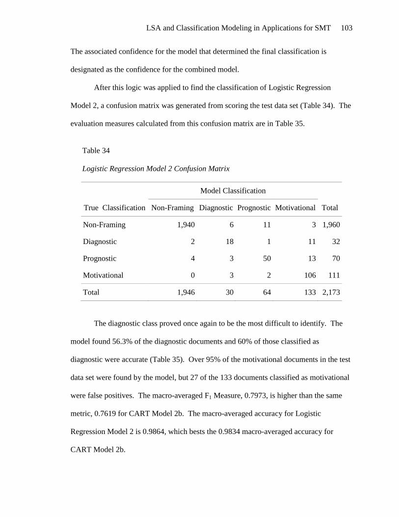
LSA and Classification Modeling in Applications for SMT 103
The associated confidence for the model that determined the final classification is
designated as the confidence for the combined model.
After this logic was applied to find the classification of Logistic Regression
Model 2, a confusion matrix was generated from scoring the test data set (Table 34). The
evaluation measures calculated from this confusion matrix are in Table 35.
Table 34
Logistic Regression Model 2 Confusion Matrix
True Classification
Model Classification
Total Non-Framing Diagnostic Prognostic Motivational
Non-Framing 1,940 6 11 3 1,960
Diagnostic 2 18 1 11 32
Prognostic 4 3 50 13 70
Motivational 0 3 2 106 111
Total 1,946 30 64 133 2,173
The diagnostic class proved once again to be the most difficult to identify. The
model found 56.3% of the diagnostic documents and 60% of those classified as
diagnostic were accurate (Table 35). Over 95% of the motivational documents in the test
data set were found by the model, but 27 of the 133 documents classified as motivational
were false positives. The macro-averaged F1 Measure, 0.7973, is higher than the same
metric, 0.7619 for CART Model 2b. The macro-averaged accuracy for Logistic
Regression Model 2 is 0.9864, which bests the 0.9834 macro-averaged accuracy for
CART Model 2b.
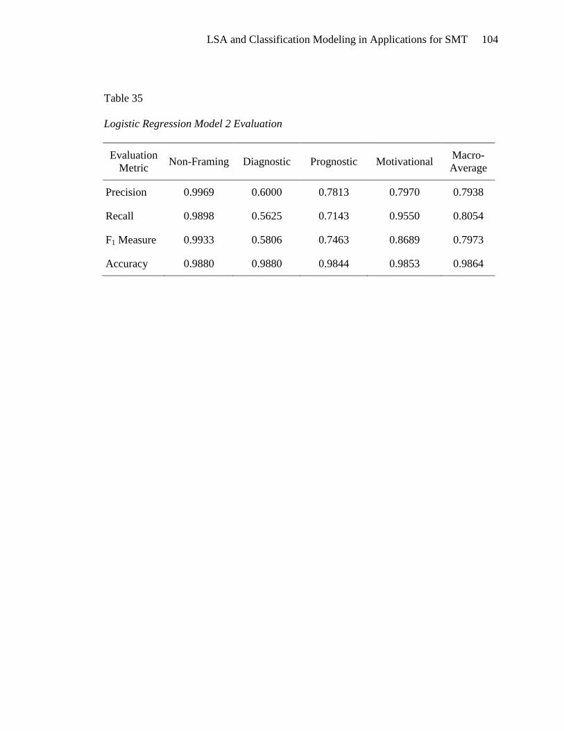
LSA and Classification Modeling in Applications for SMT 104
Table 35
Logistic Regression Model 2 Evaluation
Evaluation
Metric Non-Framing Diagnostic Prognostic Motivational
Macro-
Average
Precision 0.9969 0.6000 0.7813 0.7970 0.7938
Recall 0.9898 0.5625 0.7143 0.9550 0.8054
F1 Measure 0.9933 0.5806 0.7463 0.8689 0.7973
Accuracy 0.9880 0.9880 0.9844 0.9853 0.9864
LSA and Classification Modeling in Applications for SMT 105
Neural Network Model 2
Training: Neural Network Model 2
The target variable for Neural Network Model 2 was CAF_Name, the
polychotomous string variable used in the other Model 2 models. The predictor variables
for this model were the first thirty-five continuous SVD variables, normalized as for
Neural Network Model 1. Recall that the bivariate analysis of the SVD variables versus
the target variables revealed little value in the variables beyond SVD_35. This model was
trained using the balanced training set of documents.
Clementine reported an estimated accuracy of 95.105 for the neural network
model. The numbers of neurons were: thirty-five for the input layer, three for the hidden
layer, and four for the output layer.
Validation: Neural Network Model 2
The unbalanced test data set was scored by Neural Network Model 2. The
resulting confusion matrix is displayed in Table 36 and the evaluation measures are in
Table 37.
Once again, the diagnostic class has the lowest precision and recall. The
prognostic class also has a fairly low recall, returning 64.3% of the prognostic documents
in the test data set. For the motivational class, the model returned over 96% of the
motivational documents in the test data set and 82% of the documents classified as
motivational were correct. The macro-averaged F1 measure for the Neural Network
Model 2 is 0.8221, and the accuracy is 0.9892.
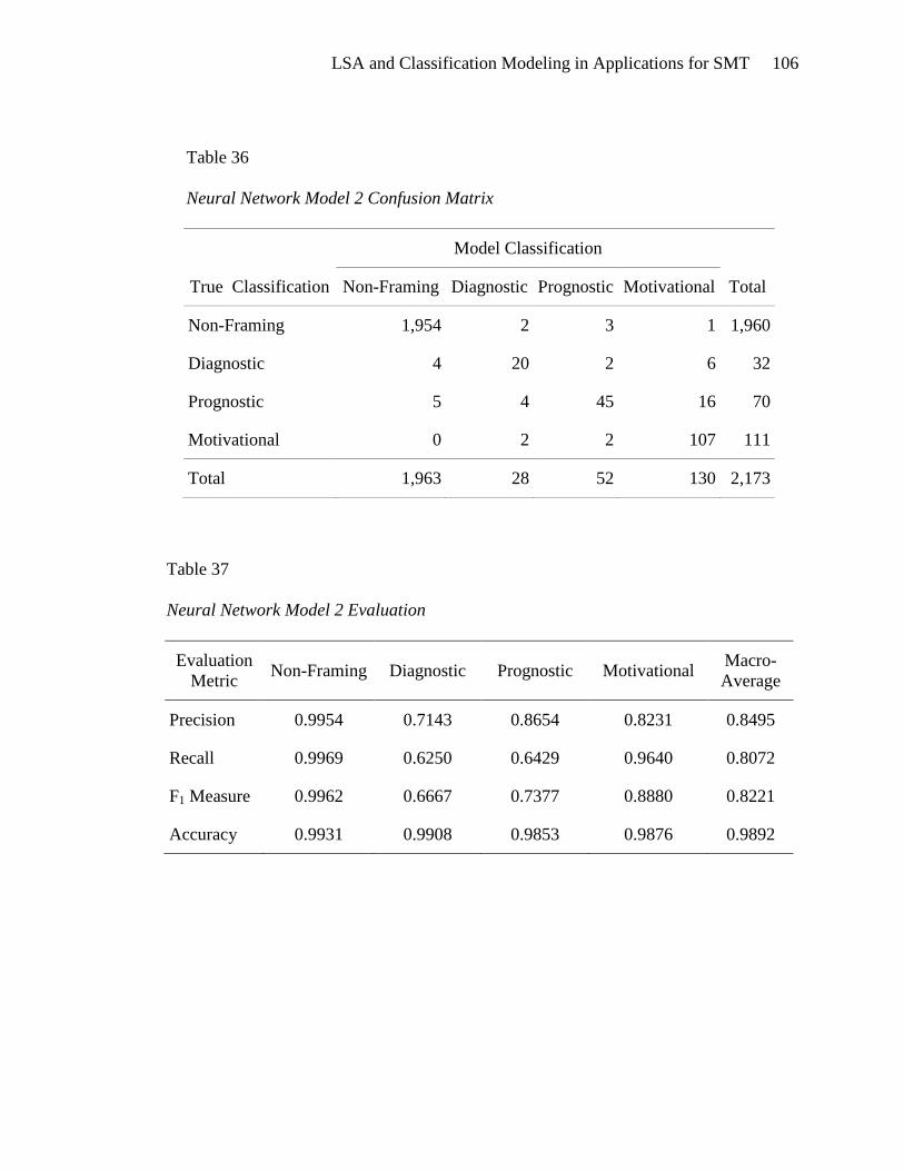
LSA and Classification Modeling in Applications for SMT 106
Table 36
Neural Network Model 2 Confusion Matrix
True Classification
Model Classification
Total Non-Framing Diagnostic Prognostic Motivational
Non-Framing 1,954 2 3 1 1,960
Diagnostic 4 20 2 6 32
Prognostic 5 4 45 16 70
Motivational 0 2 2 107 111
Total 1,963 28 52 130 2,173
Table 37
Neural Network Model 2 Evaluation
Evaluation
Metric Non-Framing Diagnostic Prognostic Motivational
Macro-
Average
Precision 0.9954 0.7143 0.8654 0.8231 0.8495
Recall 0.9969 0.6250 0.6429 0.9640 0.8072
F1 Measure 0.9962 0.6667 0.7377 0.8880 0.8221
Accuracy 0.9931 0.9908 0.9853 0.9876 0.9892
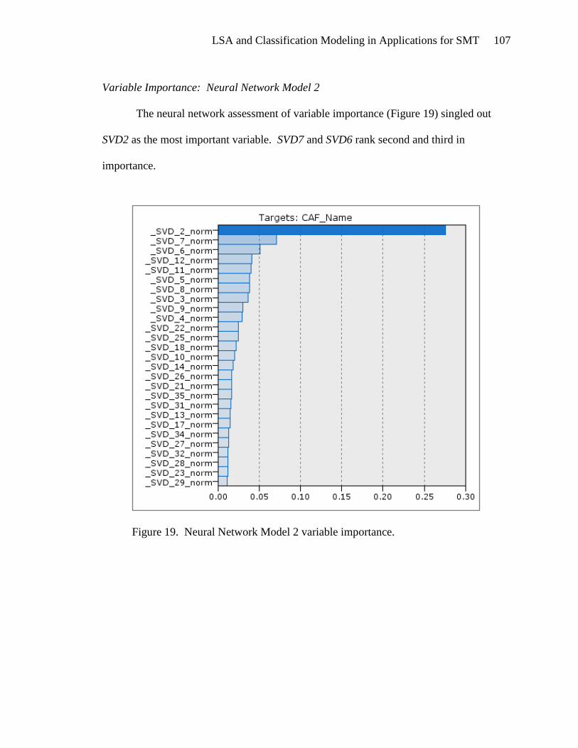
LSA and Classification Modeling in Applications for SMT 107
Variable Importance: Neural Network Model 2
The neural network assessment of variable importance (Figure 19) singled out
SVD2 as the most important variable. SVD7 and SVD6 rank second and third in
importance.
Figure 19. Neural Network Model 2 variable importance.
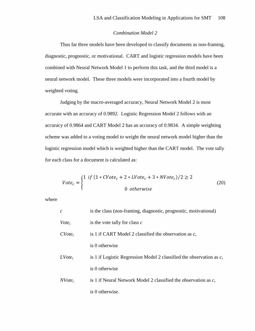
LSA and Classification Modeling in Applications for SMT 108
Combination Model 2
Thus far three models have been developed to classify documents as non-framing,
diagnostic, prognostic, or motivational. CART and logistic regression models have been
combined with Neural Network Model 1 to perform this task, and the third model is a
neural network model. These three models were incorporated into a fourth model by
weighted voting.
Judging by the macro-averaged accuracy, Neural Network Model 2 is most
accurate with an accuracy of 0.9892. Logistic Regression Model 2 follows with an
accuracy of 0.9864 and CART Model 2 has an accuracy of 0.9834. A simple weighting
scheme was added to a voting model to weight the neural network model higher than the
logistic regression model which is weighted higher than the CART model. The vote tally
for each class for a document is calculated as:
(20)
where
c is the class (non-framing, diagnostic, prognostic, motivational)
Votec is the vote tally for class c
CVotec is 1 if CART Model 2 classified the observation as c,
is 0 otherwise
LVotec is 1 if Logistic Regression Model 2 classified the observation as c,
is 0 otherwise
NVotec is 1 if Neural Network Model 2 classified the observation as c,
is 0 otherwise.
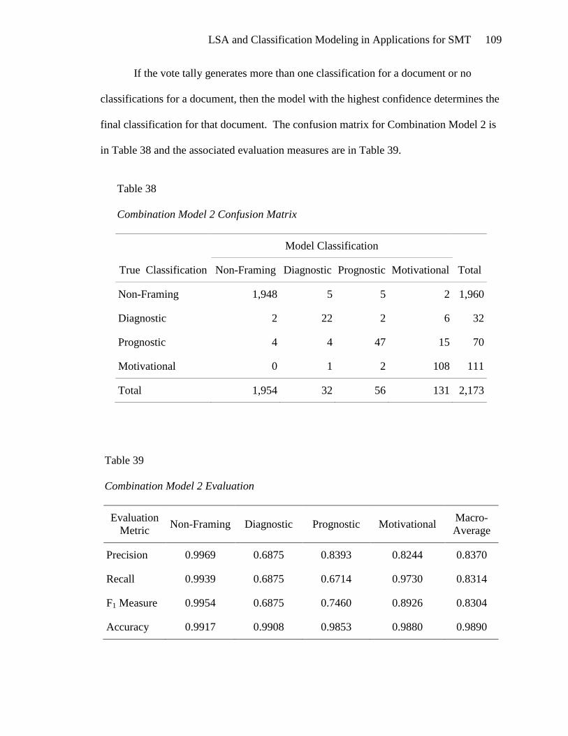
LSA and Classification Modeling in Applications for SMT 109
If the vote tally generates more than one classification for a document or no
classifications for a document, then the model with the highest confidence determines the
final classification for that document. The confusion matrix for Combination Model 2 is
in Table 38 and the associated evaluation measures are in Table 39.
Table 38
Combination Model 2 Confusion Matrix
True Classification
Model Classification
Total Non-Framing Diagnostic Prognostic Motivational
Non-Framing 1,948 5 5 2 1,960
Diagnostic 2 22 2 6 32
Prognostic 4 4 47 15 70
Motivational 0 1 2 108 111
Total 1,954 32 56 131 2,173
Table 39
Combination Model 2 Evaluation
Evaluation
Metric Non-Framing Diagnostic Prognostic Motivational
Macro-
Average
Precision 0.9969 0.6875 0.8393 0.8244 0.8370
Recall 0.9939 0.6875 0.6714 0.9730 0.8314
F1 Measure 0.9954 0.6875 0.7460 0.8926 0.8304
Accuracy 0.9917 0.9908 0.9853 0.9880 0.9890
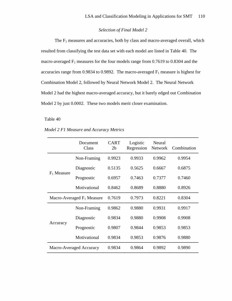
LSA and Classification Modeling in Applications for SMT 110
Selection of Final Model 2
The F1 measures and accuracies, both by class and macro-averaged overall, which
resulted from classifying the test data set with each model are listed in Table 40. The
macro-averaged F1 measures for the four models range from 0.7619 to 0.8304 and the
accuracies range from 0.9834 to 0.9892. The macro-averaged F1 measure is highest for
Combination Model 2, followed by Neural Network Model 2. The Neural Network
Model 2 had the highest macro-averaged accuracy, but it barely edged out Combination
Model 2 by just 0.0002. These two models merit closer examination.
Table 40
Model 2 F1 Measure and Accuracy Metrics
Document
Class
CART
2b
Logistic
Regression
Neural
Network Combination
F1 Measure
Non-Framing 0.9923 0.9933 0.9962 0.9954
Diagnostic 0.5135 0.5625 0.6667 0.6875
Prognostic 0.6957 0.7463 0.7377 0.7460
Motivational 0.8462 0.8689 0.8880 0.8926
Macro-Averaged F1 Measure 0.7619 0.7973 0.8221 0.8304
Accuracy
Non-Framing 0.9862 0.9880 0.9931 0.9917
Diagnostic 0.9834 0.9880 0.9908 0.9908
Prognostic 0.9807 0.9844 0.9853 0.9853
Motivational 0.9834 0.9853 0.9876 0.9880
Macro-Averaged Accuracy 0.9834 0.9864 0.9892 0.9890

LSA and Classification Modeling in Applications for SMT 111
The confusion matrices for both models are displayed together in Table 41 for
comparison. An additional column, “% Found,” has been added to the matrices. This is
the recall measure expressed as a percentage. As discussed in the consideration of Model
1, the intended use for the model should guide model selection. If overall accuracy is of
paramount importance, then Neural Network Model 2 is best although it barely edges out
its competition. If the purpose of the model is to filter these three types of framing
documents from a flood of Internet posts and present the results to humans who assess
risks associated with collective action, then Combination Model 2 discovered higher
proportions of all three types of framing documents than Neural Network Model 2, but at
a slight cost. The false positive rates from Combination Model 2 are higher than Neural
Network Model 2 for the diagnostic and prognostic classes. The macro-averaged F1
measures reflect these differences between the two models. The analyst may be willing
to tolerate additional false positives rather than risk losing one motivational document
that completes the picture. In that case, Combination Model 2 would be chosen as the
final model.
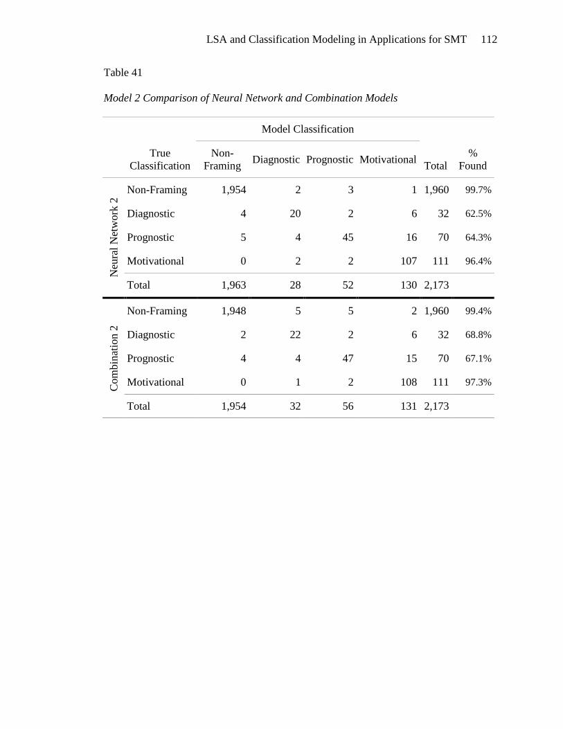
LSA and Classification Modeling in Applications for SMT 112
Table 41
Model 2 Comparison of Neural Network and Combination Models
True
Classification
Model Classification
Total
Non-
Framing Diagnostic Prognostic Motivational
%
Found
Neu
ral
Net
work
2 Non-Framing 1,954 2 3 1 1,960 99.7%
Diagnostic 4 20 2 6 32 62.5%
Prognostic 5 4 45 16 70 64.3%
Motivational 0 2 2 107 111 96.4%
Total 1,963 28 52 130 2,173
Com
bin
atio
n 2
Non-Framing 1,948 5 5 2 1,960 99.4%
Diagnostic 2 22 2 6 32 68.8%
Prognostic 4 4 47 15 70 67.1%
Motivational 0 1 2 108 111 97.3%
Total 1,954 32 56 131 2,173
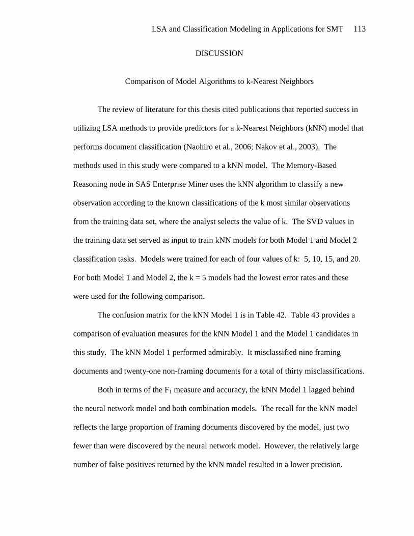
LSA and Classification Modeling in Applications for SMT 113
DISCUSSION
Comparison of Model Algorithms to k-Nearest Neighbors
The review of literature for this thesis cited publications that reported success in
utilizing LSA methods to provide predictors for a k-Nearest Neighbors (kNN) model that
performs document classification (Naohiro et al., 2006; Nakov et al., 2003). The
methods used in this study were compared to a kNN model. The Memory-Based
Reasoning node in SAS Enterprise Miner uses the kNN algorithm to classify a new
observation according to the known classifications of the k most similar observations
from the training data set, where the analyst selects the value of k. The SVD values in
the training data set served as input to train kNN models for both Model 1 and Model 2
classification tasks. Models were trained for each of four values of k: 5, 10, 15, and 20.
For both Model 1 and Model 2, the k = 5 models had the lowest error rates and these
were used for the following comparison.
The confusion matrix for the kNN Model 1 is in Table 42. Table 43 provides a
comparison of evaluation measures for the kNN Model 1 and the Model 1 candidates in
this study. The kNN Model 1 performed admirably. It misclassified nine framing
documents and twenty-one non-framing documents for a total of thirty misclassifications.
Both in terms of the F1 measure and accuracy, the kNN Model 1 lagged behind
the neural network model and both combination models. The recall for the kNN model
reflects the large proportion of framing documents discovered by the model, just two
fewer than were discovered by the neural network model. However, the relatively large
number of false positives returned by the kNN model resulted in a lower precision.
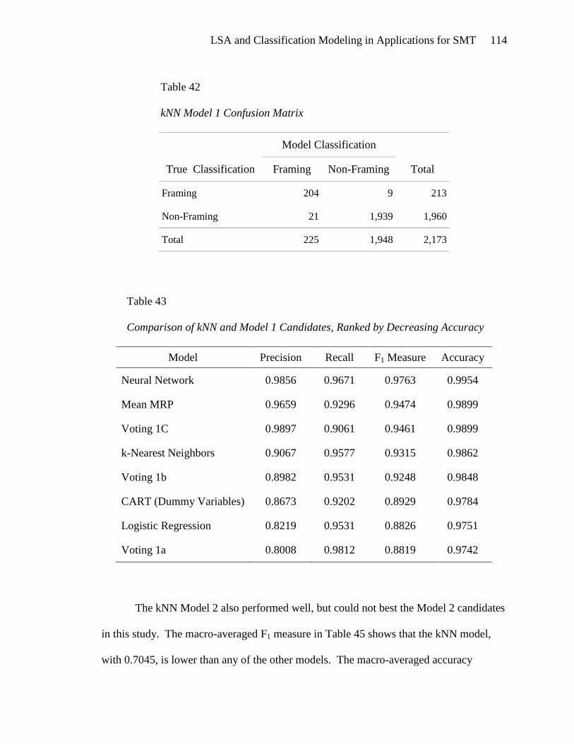
LSA and Classification Modeling in Applications for SMT 114
Table 42
kNN Model 1 Confusion Matrix
True Classification
Model Classification
Total Framing Non-Framing
Framing 204 9 213
Non-Framing 21 1,939 1,960
Total 225 1,948 2,173
Table 43
Comparison of kNN and Model 1 Candidates, Ranked by Decreasing Accuracy
Model Precision Recall F1 Measure Accuracy
Neural Network 0.9856 0.9671 0.9763 0.9954
Mean MRP 0.9659 0.9296 0.9474 0.9899
Voting 1C 0.9897 0.9061 0.9461 0.9899
k-Nearest Neighbors 0.9067 0.9577 0.9315 0.9862
Voting 1b 0.8982 0.9531 0.9248 0.9848
CART (Dummy Variables) 0.8673 0.9202 0.8929 0.9784
Logistic Regression 0.8219 0.9531 0.8826 0.9751
Voting 1a 0.8008 0.9812 0.8819 0.9742
The kNN Model 2 also performed well, but could not best the Model 2 candidates
in this study. The macro-averaged F1 measure in Table 45 shows that the kNN model,
with 0.7045, is lower than any of the other models. The macro-averaged accuracy
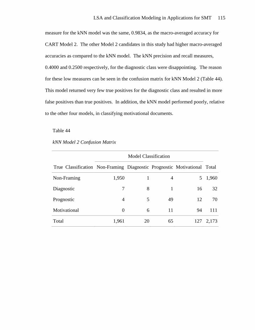
LSA and Classification Modeling in Applications for SMT 115
measure for the kNN model was the same, 0.9834, as the macro-averaged accuracy for
CART Model 2. The other Model 2 candidates in this study had higher macro-averaged
accuracies as compared to the kNN model. The kNN precision and recall measures,
0.4000 and 0.2500 respectively, for the diagnostic class were disappointing. The reason
for these low measures can be seen in the confusion matrix for kNN Model 2 (Table 44).
This model returned very few true positives for the diagnostic class and resulted in more
false positives than true positives. In addition, the kNN model performed poorly, relative
to the other four models, in classifying motivational documents.
Table 44
kNN Model 2 Confusion Matrix
True Classification
Model Classification
Total Non-Framing Diagnostic Prognostic Motivational
Non-Framing 1,950 1 4 5 1,960
Diagnostic 7 8 1 16 32
Prognostic 4 5 49 12 70
Motivational 0 6 11 94 111
Total 1,961 20 65 127 2,173
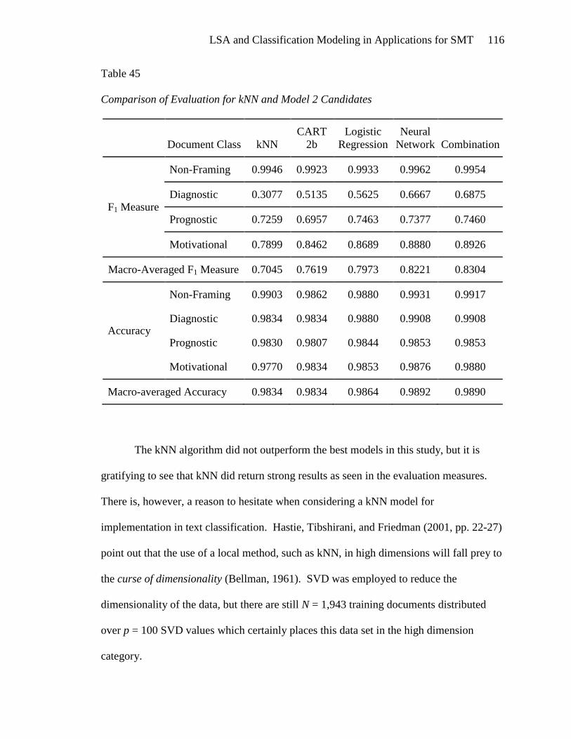
LSA and Classification Modeling in Applications for SMT 116
Table 45
Comparison of Evaluation for kNN and Model 2 Candidates
Document Class kNN
CART
2b
Logistic
Regression
Neural
Network Combination
F1 Measure
Non-Framing 0.9946 0.9923 0.9933 0.9962 0.9954
Diagnostic 0.3077 0.5135 0.5625 0.6667 0.6875
Prognostic 0.7259 0.6957 0.7463 0.7377 0.7460
Motivational 0.7899 0.8462 0.8689 0.8880 0.8926
Macro-Averaged F1 Measure 0.7045 0.7619 0.7973 0.8221 0.8304
Accuracy
Non-Framing 0.9903 0.9862 0.9880 0.9931 0.9917
Diagnostic 0.9834 0.9834 0.9880 0.9908 0.9908
Prognostic 0.9830 0.9807 0.9844 0.9853 0.9853
Motivational 0.9770 0.9834 0.9853 0.9876 0.9880
Macro-averaged Accuracy 0.9834 0.9834 0.9864 0.9892 0.9890
The kNN algorithm did not outperform the best models in this study, but it is
gratifying to see that kNN did return strong results as seen in the evaluation measures.
There is, however, a reason to hesitate when considering a kNN model for
implementation in text classification. Hastie, Tibshirani, and Friedman (2001, pp. 22-27)
point out that the use of a local method, such as kNN, in high dimensions will fall prey to
the curse of dimensionality (Bellman, 1961). SVD was employed to reduce the
dimensionality of the data, but there are still N = 1,943 training documents distributed
over p = 100 SVD values which certainly places this data set in the high dimension
category.
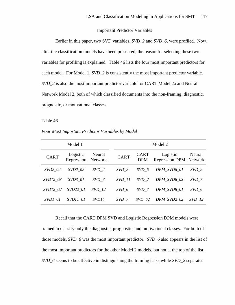
LSA and Classification Modeling in Applications for SMT 117
Important Predictor Variables
Earlier in this paper, two SVD variables, SVD_2 and SVD_6, were profiled. Now,
after the classification models have been presented, the reason for selecting these two
variables for profiling is explained. Table 46 lists the four most important predictors for
each model. For Model 1, SVD_2 is consistently the most important predictor variable.
SVD_2 is also the most important predictor variable for CART Model 2a and Neural
Network Model 2, both of which classified documents into the non-framing, diagnostic,
prognostic, or motivational classes.
Table 46
Four Most Important Predictor Variables by Model
Model 1 Model 2
CART Logistic
Regression
Neural
Network
CART
CART
DPM
Logistic
Regression DPM
Neural
Network
SVD2_02 SVD2_02 SVD_2 SVD_2 SVD_6 DPM_SVD6_01 SVD_2
SVD12_03 SVD3_01 SVD_7 SVD_11 SVD_2 DPM_SVD6_03 SVD_7
SVD12_02 SVD22_01 SVD_12 SVD_6 SVD_7 DPM_SVD8_01 SVD_6
SVD1_01 SVD11_01 SVD14 SVD_7 SVD_62 DPM_SVD2_02 SVD_12
Recall that the CART DPM SVD and Logistic Regression DPM models were
trained to classify only the diagnostic, prognostic, and motivational classes. For both of
those models, SVD_6 was the most important predictor. SVD_6 also appears in the list of
the most important predictors for the other Model 2 models, but not at the top of the list.
SVD_6 seems to be effective in distinguishing the framing tasks while SVD_2 separates
LSA and Classification Modeling in Applications for SMT 118
framing and non-framing texts. The profiling of these two variables provided evidence to
back up this assumption.
The Difficulty of Classification
In this study, all of the documents address one topic, Global Warming, and the
task is to detect those documents that were written for the purpose of influencing
perceptions and actions regarding the topic. This task is made more challenging when
one considers the fact that both non-framing and diagnostic framing texts can define
climate change and its effect on our planet. The subtle difference is that the non-framing
document may have been written for the purpose of educating the reader, while the
diagnostic framing document is intended to not only educate, but also influence the
reader‟s perception of events and personal experience. In the same manner, elements of
prognostic framing text may logically be found in non-framing text. Morrow et al.
(2008), in discussing their research involving classifying Senate speeches by political
party, mention the challenging nature of ideological classification, “… it seems that a
more ideologically-based classification might be a more difficult problem than
classifying by author – often, Democrats and Republicans use the same words but are
discussing very different ideas” (p. 8).

LSA and Classification Modeling in Applications for SMT 119
CONCLUSION
The accuracy of the methods employed in this study was excellent. For the model
that distinguished framing from non-framing documents, the accuracies ranged from
97.5% to 99.5%. Likewise, the polychotomous models, which identified non-framing
versus diagnostic versus prognostic versus motivational documents, had accuracies
ranging from 98.3% to 98.9%. To place these results in perspective, the literature review
identified a study that had a similar goal of classifying ideology in text documents. That
paper reported best accuracies for a dichotomous target variable in the 85% to 92%
range, and other model accuracies ranging from 70% to 90% as being acceptable
(Morrow et al. 2008, Figure 4, p. 7). A polychotomous model was not addressed in that
study.
The fact that this study has been successful in demonstrating that framing
documents can be accurately distinguished from non-framing documents lends credence
to the theory that framing involves distinct and identifiable language characteristics.
Moreover, the successful classification of framing documents by core framing task, with
high accuracy, provides the means to measure these fine distinctions. From the results
seen here, one may presume that social scientists can use these techniques to further the
study, measurement, and validation of current thinking regarding the framing efforts of
Social Movement Organizations.
Latent Semantic Analysis techniques were shown to be effective in providing
robust predictor variables for the classification models. The neural network modeling
algorithm performed well for both models, but it was a combination model that excelled
in the more difficult problem of finding documents belonging to specific framing tasks.
LSA and Classification Modeling in Applications for SMT 120
This study could have failed to accomplish the goal of developing classification
models to discover framing documents. The problem is difficult. Moreover, the tenets of
Social Movement Theory upon which this thesis rests, have been developed through
observation and analysis with less emphasis on quantification. This is understandable,
indeed necessary, when one considers the topic is dependent upon human nature, not
physical science. Major Jennifer Chandler, USAF, notes that “Research has
predominately focused on understanding why and how frames generate resonance”
(Chandler, 2005). She then explains the need for framing research to conduct studies to
better define the mechanisms of framing processes.
Future Work
The corpus of documents was split into training and test data sets. When data are
plentiful, partitioning the corpus into training, validation, and test data sets is the accepted
practice. In that case, the error on the validation data set aids in model selection, and the
test data set provides the estimation of predictive error on new data (Hastie et al., 2001, p.
196). The small number of framing documents, by core task, used in this corpus,
necessitated the use of just training and test data sets. Cross-validation and bootstrap
methods are designed to estimate prediction error when the environment is not data rich.
Incorporating one or both of these methods may present a more realistic estimate of the
accuracy of the models.
Some writers of framing texts are becoming more sophisticated in their frame
construction by adopting a reasonable rather than a rhetorical tone (Benjamin, 2007).
Benjamin posits that a rhetorical tone is patronizing, dogmatic, and biased. Her research
indicates that people respond to a rhetorical tone with skepticism and resistance. In

LSA and Classification Modeling in Applications for SMT 121
contrast, she paints a reasonable tone as non-argumentative, optimistic, and based upon
widely accepted values. In this case, Benjamin theorizes that the reader is more likely to
be encouraged and to start thinking about solving the issues. Future work can be
undertaken to adopt the approach that was demonstrated in this study for the
identification of tone in framing documents, thus singling out those that are more apt to
be successful in recruiting followers.
LSA and Classification Modeling in Applications for SMT 122
REFERENCES
Anderson, R. (2007). The credit scoring toolkit: Theory and practice for retail credit risk
management and decision automation. USA: Oxford University Press.
BBC News. (2001). Summit fails to solve climate dispute. Retrieved September 8, 2008,
from http://news.bbc.co.uk/1/hi/world/europe/1387667.stm
Bellman, R. E. (1961). Adaptive control processes. Princeton University Press.
Benjamin, D. (2007, December). Finding a reasonable tone. Retrieved January 5, 2009,
from FrameWorks Institute: http://www.frameworksinstitute.org/framebytes.html
Bilisoly, R. (2008). Practical text mining with Perl. Hoboken, NJ: John Wiley & Sons,
Inc.
Breiman, L., Friedman, J., Olshen, R., & Stone, C. (1984). Classification and regression
trees. Boca Raton, FL: Chapman & Hall/CRC Press.
Campbell, P. (2008, July 6). Image:2008-07 climate rally human sign 2.jpg. Retrieved
November 17, 2009, from Greenlivingpedia:
http://www.greenlivingpedia.org/Image:2008-
07_climate_rally_human_sign_2.jpg
Chandler, J. (2005, May). The explanatory value of social movement theory. Strategic
Insights , IV (5).
Climate Action Network Australia. (2008). Mission. Retrieved September 9, 2008, from
http://www.cana.net.au/index.php?site_var=12
Climate Camp. (2008). Camp for climate action Australia. Retrieved May 19, 2008, from
http://www.climatecamp.org.au/
LSA and Classification Modeling in Applications for SMT 123
Climate Rally. (2008). Climate emergency rally. Retrieved May 20, 2008, from
http://climaterally.blogspot.com/
Communist Party USA. (2008). Global warming - the communist solution. Retrieved
September 9, 2008, from http://www.cpusa.org/article/view/933/
Cooper, A. (2002). Media framing and social movement mobilization: German peace
protest against INF missiles, the Gulf War, and NATO peace enforcement in
Bosnia. European Journal of Political Research , 41, 37-80.
Courtice, B. (2008, July 5). Thank you and well done. Retrieved November 17, 2008,
from CLIMATE CRIMINALS TOUR OF MELBOURNE: Climate Emergency
Rally:
http://climaterally.blogspot.com/search/label/Climate%20Emergency%20Rally
Deerwester, S., Dumais, S., Furnas, G., Landauer, T., & Harshman, R. (1990). Indexing
by latent semantic analysis. Journal of the American Society for Information
Science , 41 (6), 391-407.
Della Porta, D., & Diani, M. (1999). Social movements: An introduction. Oxford:
Blackwell Publishers.
FrameWorks. (n.d.). FrameWorks issues: Global warming. Retrieved January 5, 2009,
from The FrameWorks Institute Web Site:
http://www.frameworksinstitute.org/globalwarming.html
FrameWorks. (1999). Mission of the FrameWorks Institute. Retrieved January 5, 2009,
from The FrameWorks Institute Web Site:
http://www.frameworksinstitute.org/mission.html
LSA and Classification Modeling in Applications for SMT 124
Goffman, E. (1974). Frame analysis: An essay on the organization of experience. New
York, NY: Harper & Row.
Hastie, T., Tibshirani, R., & Friedman, J. (2001). The Elements of Statistical Learning.
New York, NY: Springer-Verlag.
Hosmer, D. W., & Lemeshow, S. (2000). Applied logistic regression (2 ed.). Hoboken,
NJ: John Wiley & Sons, Inc.
ISI Web of Knowledge. (2008). Thomson Reuters.
Koenig, T. (2005). Routinizing frame analysis. Proceedings of the ISA RC-33
Methodology Conference. Leverkusen: Leske & Budrich.
Landauer, T. K., Foltz, P. W., & Laham, D. (1998). An introduction to latent semantic
analysis. Discourse Processes , 25, 259-284.
Larose, D. (2006). Data mining methods and models. Hoboken, NJ: John Wiley & Sons.
Larose, D. (2005). Discovering knowledge in data. Hoboken, NJ: John Wiley & Sons.
Manning, C. D., & Schütze, H. (1999). Foundations of statistical natural language
processing. Cambridge, MA: The MIT Press.
Manning, C. D., Raghavan, P., & Schütze, H. (2008). Introduction to information
retrieval. New York, NY: Cambridge University Press.
McAdam, D., McCarthy, J., & Zald, M. (1988). Social movements. In N. Smelser (Ed.),
Handbook of sociology. Thousand Oaks, CA: Sage Publications.
Morrow, J., Bader, B., Chew, P., & Speed, A. (2008). Ideological determination using
small amounts of text. International Studies Association 49th Annual Convention.
San Francisco, CA.
LSA and Classification Modeling in Applications for SMT 125
Nakov, P., Valchanova, E., & Angelova, G. (2003). Towards deeper understanding of the
LSA performance. Proc. Recent Advances in Natural Language, (pp. 311-318).
Borovetz, Bulgaria.
Naohiro, I., Murai, T., Yamada, T., & Bao, Y. (2006). Text classification by combining
grouping, LSA and kNN. Proceedings from 5th IEEE/ACIS ICIS-COMSAR '06.
Los Alamitos, CA: IEEE Computer Society.
New Europe. (2008, June 16). Saudi Arabia joins global warming fight scheme.
Retrieved September 9, 2008, from http://www.neurope.eu/articles/87683.php
Pyle, D. (2003). Business modeling and data mining. San Francisco, CA: Morgan
Kaufmann.
Reuters. (2008). Protesters disrupt loading at Australian coal port. Retrieved September
8, 2008, from
http://www.reuters.com/article/rbssMiningMetalsSpecialty/idUSSYD1146922008
0714
Rising Tide. (2008, February 26). Topple the fossil fuel empire. Retrieved June 9, 2008,
from risingtide.org.uk:
http://risingtide.org.uk/files/rt/15%20Actions%20to%20Topple%20the%20Fossil
%20Fuel%20Empire%20-%20Web%20Version.pdf
SAS Institute, Inc. (2003). Descriptive terms of clusters. Text Miner Node . Cary, NC.
SAS Institute, Inc. (2003). Weighting methods. Text Miner Node . Cary, NC.
LSA and Classification Modeling in Applications for SMT 126
SAS® Enterprise Miner™. (2003-2005). Version 2.3 of the SAS System for Windows,
copyright © 2003 - 2005 SAS Institute Inc. SAS and all other SAS Institute Inc.
product or service names are registered trademarks or trademarks of SAS
Institute Inc., Cary, NC, USA.
SAS® Software. (2002-2003). Version 9.1.3 of the SAS System for Windows, copyright ©
2002 - 2003 SAS Institute Inc. SAS and all other SAS Institute Inc. product or
service names are registered trademarks or trademarks of SAS Institute Inc.,
Cary, NC, USA.
SAS® Text Miner. (2003-2005). Version 2.3 of the SAS System for Windows, copyright
© 2003 - 2005 SAS Institute Inc. SAS and all other SAS Institute Inc. product or
service names are registered trademarks or trademarks of SAS Institute Inc.,
Cary, NC, USA.
Semetko, H., & Valkenburg, P. (2000). Framing European politics: a content analysis of
press and television news. Journal of Communication , 50 (2), 93-109.
Shao, G. (1994). Potential impacts of climate change on a mixed broadleaved-Korean
pine forest stand: A gap model approach. International-Geosphere-Biosphere-
Program Workshop on the Application of Forest-Stand-Models-to-Global-
Change-Issues. Apeldoorn Netherlands: Kluwer Academic Publ.
Sierra Club. (2008). Global warming policy solutions. Retrieved May 14, 2008, from
http://www.sierraclub.org/energy/energypolicy/
Snow, D., & Benford, R. (1988). Ideology, frame resonance and participant mobilization.
International Social Movement Research , 1, 197-219.

LSA and Classification Modeling in Applications for SMT 127
Southern Baptist Convention. (2007). SBC resolutions: On global warming. Retrieved
September 9, 2008, from
http://www.sbc.net/resolutions/amResolution.asp?ID=1171
SPSS Clementine®. (2007). Rel. 12.0.1 SPSS, Incorporated. Chicago, IL.
Triandafyllidou, A., & Fotiou, A. (1998). Sustainability and modernity in the European
Union: A frame theory approach on policy-making. Sociological Research Online
, 3 (1).
World Development Movement. (2008). No new coal - stop Kingsnorth. Retrieved May
19, 2008, from World Development Movement Campaigns:
http://www.wdm.org.uk/campaigns/climate/action/kingsnorth.htm

LSA and Classification Modeling in Applications for SMT 128
BIOGRAPHICAL STATEMENT
Judith Spomer is a Senior Member of Technical Staff at Sandia National
Laboratories1 in Albuquerque, New Mexico. She holds a B.S in Computer Science from
Indiana University of Pennsylvania. During her career she has worked as a process
control engineer, software engineer, and credit risk modeler in the chemical and financial
services industries. Mrs. Spomer is married with four children and makes her home in
Tijeras, NM.
1 Sandia is a multiprogram laboratory operated by Sandia Corporation, a Lockheed Martin
Company, for the United States Department of Energy‟s National Nuclear Security Administration under
Contract DE-AC04-94AL85000.
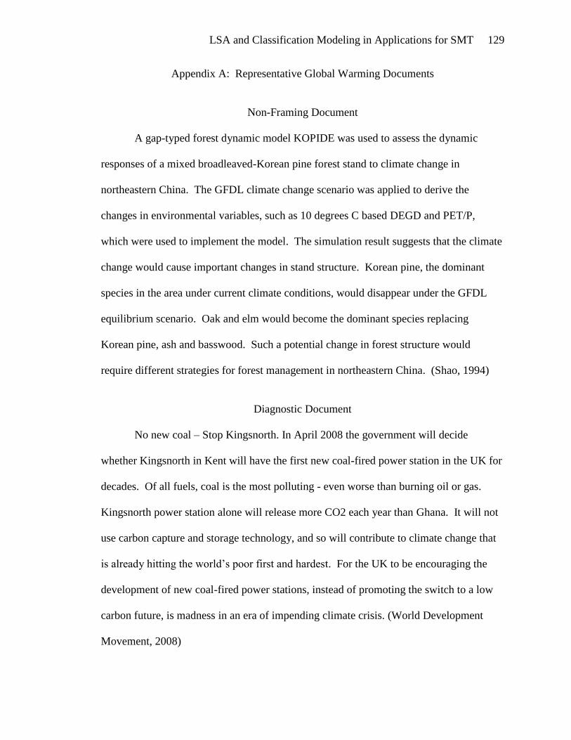
LSA and Classification Modeling in Applications for SMT 129
Appendix A: Representative Global Warming Documents
Non-Framing Document
A gap-typed forest dynamic model KOPIDE was used to assess the dynamic
responses of a mixed broadleaved-Korean pine forest stand to climate change in
northeastern China. The GFDL climate change scenario was applied to derive the
changes in environmental variables, such as 10 degrees C based DEGD and PET/P,
which were used to implement the model. The simulation result suggests that the climate
change would cause important changes in stand structure. Korean pine, the dominant
species in the area under current climate conditions, would disappear under the GFDL
equilibrium scenario. Oak and elm would become the dominant species replacing
Korean pine, ash and basswood. Such a potential change in forest structure would
require different strategies for forest management in northeastern China. (Shao, 1994)
Diagnostic Document
No new coal – Stop Kingsnorth. In April 2008 the government will decide
whether Kingsnorth in Kent will have the first new coal-fired power station in the UK for
decades. Of all fuels, coal is the most polluting - even worse than burning oil or gas.
Kingsnorth power station alone will release more CO2 each year than Ghana. It will not
use carbon capture and storage technology, and so will contribute to climate change that
is already hitting the world‟s poor first and hardest. For the UK to be encouraging the
development of new coal-fired power stations, instead of promoting the switch to a low
carbon future, is madness in an era of impending climate crisis. (World Development
Movement, 2008)

LSA and Classification Modeling in Applications for SMT 130
Prognostic Document
Reduce emissions to avoid dangerous global warming: Scientists tell us that we
must cut greenhouse gas emissions by at least 80% by 2050 to prevent global
temperatures from rising more than 2º C over pre-industrial averages. Not only must
global warming policy require such emissions reductions, but it must also ensure the U.S.
adheres to this mandate by requiring periodic scientific review of progress toward
sufficient emission reductions that will meet this goal. Legislation should direct EPA to
adjust its regulatory process based on future scientific study and review of climate change
to ensure that we meet measurable, intermittent emission reduction benchmarks between
now and 2050 that will prevent a rise in global temperatures above dangerous levels.
(Sierra Club, 2008)
Motivational Document
Welcome to Climate Camp Australia. The camp for climate action will be five
days of inspiring workshops & direct action aimed at shutting down the world's largest
coal port in Newcastle, just north of Sydney. If you are concerned about climate change,
and want real action instead of more hot air, then we encourage you to come, bring your
friends and family and get involved. Whether you are old or young, a seasoned protestor
or if you've never been to a protest in your life, if you share our passion for climate
action, then climate camp is for you! We'd love for you to get involved and help make
the camp as big, bold and effective as possible. Whatever your background, there is a
role for you. Find out more about how you can get involved. (Climate Camp, 2008)
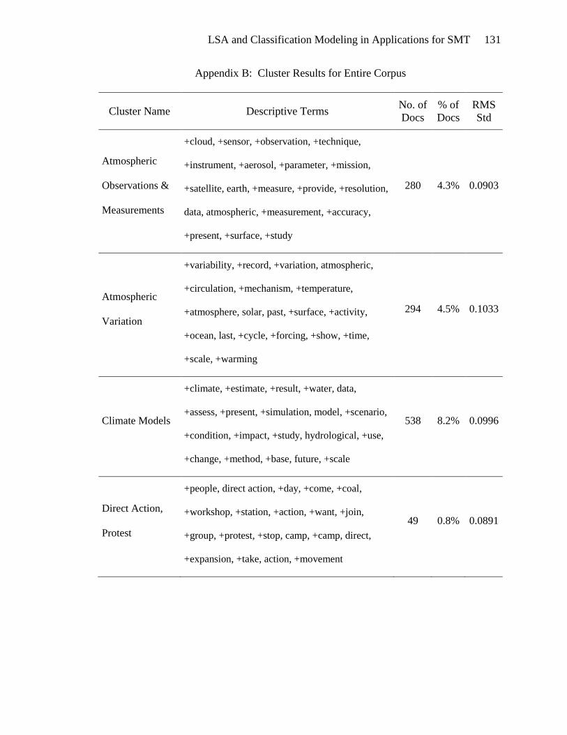
LSA and Classification Modeling in Applications for SMT 131
Appendix B: Cluster Results for Entire Corpus
Cluster Name Descriptive Terms No. of
Docs
% of
Docs
RMS
Std
Atmospheric
Observations &
Measurements
+cloud, +sensor, +observation, +technique,
+instrument, +aerosol, +parameter, +mission,
+satellite, earth, +measure, +provide, +resolution,
data, atmospheric, +measurement, +accuracy,
+present, +surface, +study
280 4.3% 0.0903
Atmospheric
Variation
+variability, +record, +variation, atmospheric,
+circulation, +mechanism, +temperature,
+atmosphere, solar, past, +surface, +activity,
+ocean, last, +cycle, +forcing, +show, +time,
+scale, +warming
294 4.5% 0.1033
Climate Models
+climate, +estimate, +result, +water, data,
+assess, +present, +simulation, model, +scenario,
+condition, +impact, +study, hydrological, +use,
+change, +method, +base, future, +scale
538 8.2% 0.0996
Direct Action,
Protest
+people, direct action, +day, +come, +coal,
+workshop, +station, +action, +want, +join,
+group, +protest, +stop, camp, +camp, direct,
+expansion, +take, action, +movement
49 0.8% 0.0891
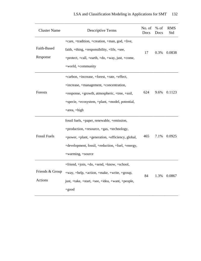
LSA and Classification Modeling in Applications for SMT 132
Cluster Name Descriptive Terms No. of
Docs
% of
Docs
RMS
Std
Faith-Based
Response
+care, +tradition, +creation, +man, god, +live,
faith, +thing, +responsibility, +life, +see,
+protect, +call, +earth, +do, +way, just, +come,
+world, +community
17 0.3% 0.0838
Forests
+carbon, +increase, +forest, +rate, +effect,
+increase, +management, +concentration,
+response, +growth, atmospheric, +tree, +soil,
+specie, +ecosystem, +plant, +model, potential,
+area, +high
624 9.6% 0.1123
Fossil Fuels
fossil fuels, +paper, renewable, +emission,
+production, +resource, +gas, +technology,
+power, +plant, +generation, +efficiency, global,
+development, fossil, +reduction, +fuel, +energy,
+warming, +source
465 7.1% 0.0925
Friends & Group
Actions
+friend, +join, +do, +send, +know, +school,
+way, +help, +action, +make, +write, +group,
just, +take, +start, +see, +idea, +want, +people,
+good
84 1.3% 0.0867

LSA and Classification Modeling in Applications for SMT 133
Cluster Name Descriptive Terms No. of
Docs
% of
Docs
RMS
Std
GHGs / Ozone
+gas, warming, +use, +process, +atmosphere,
+emission, +high, ozone, environmental, +system,
+warming, carbon dioxide, +method, +product,
+potential, +application, global, global warming,
+problem, +low
476 7.3% 0.1013
Glaciers
+snow, +extent, +sea, +balance, +glacier,
+surface, +accumulation, +summer, +cover, ice,
+temperature, +area, +record, +show, +indicate,
+variability, +region, +year, +period, +trend
247 3.8% 0.0962
Government &
Corporate
Response to GW
+help, +send, +state, +clean, +government,
renewable energy, +take, +stop, now, +efficiency,
+invest, +reduce, renewable, +company, +create,
+action, +solution, +energy, +power, +do
107 1.6% 0.0927
Effect of GW
on Human
Populations
human, +world, +food, health, +people, +country,
+population, +problem, +affect, +do, +cause,
environmental, +environment, +increase, +make,
+warming, global warming, more, +part, other
311 4.8% 0.1164
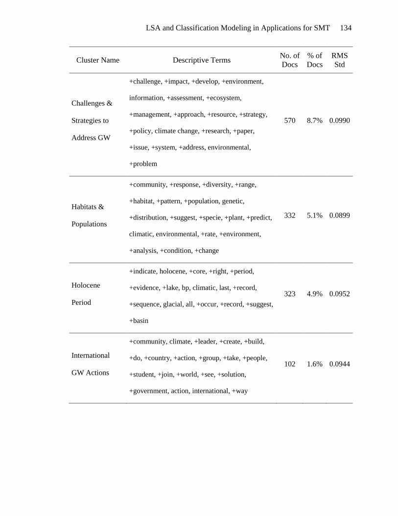
LSA and Classification Modeling in Applications for SMT 134
Cluster Name Descriptive Terms No. of
Docs
% of
Docs
RMS
Std
Challenges &
Strategies to
Address GW
+challenge, +impact, +develop, +environment,
information, +assessment, +ecosystem,
+management, +approach, +resource, +strategy,
+policy, climate change, +research, +paper,
+issue, +system, +address, environmental,
+problem
570 8.7% 0.0990
Habitats &
Populations
+community, +response, +diversity, +range,
+habitat, +pattern, +population, genetic,
+distribution, +suggest, +specie, +plant, +predict,
climatic, environmental, +rate, +environment,
+analysis, +condition, +change
332 5.1% 0.0899
Holocene
Period
+indicate, holocene, +core, +right, +period,
+evidence, +lake, bp, climatic, last, +record,
+sequence, glacial, all, +occur, +record, +suggest,
+basin
323 4.9% 0.0952
International
GW Actions
+community, climate, +leader, +create, +build,
+do, +country, +action, +group, +take, +people,
+student, +join, +world, +see, +solution,
+government, action, international, +way
102 1.6% 0.0944
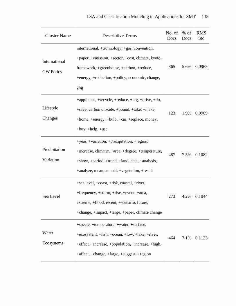
LSA and Classification Modeling in Applications for SMT 135
Cluster Name Descriptive Terms No. of
Docs
% of
Docs
RMS
Std
International
GW Policy
international, +technology, +gas, convention,
+paper, +emission, +sector, +cost, climate, kyoto,
framework, +greenhouse, +carbon, +reduce,
+energy, +reduction, +policy, economic, change,
ghg
365 5.6% 0.0965
Lifestyle
Changes
+appliance, +recycle, +reduce, +big, +drive, +do,
+save, carbon dioxide, +pound, +take, +make,
+home, +energy, +bulb, +car, +replace, money,
+buy, +help, +use
123 1.9% 0.0909
Precipitation
Variation
+year, +variation, +precipitation, +region,
+increase, climatic, +area, +degree, +temperature,
+show, +period, +trend, +land, data, +analysis,
+analyze, mean, annual, +vegetation, +result
487 7.5% 0.1082
Sea Level
+sea level, +coast, +risk, coastal, +river,
+frequency, +storm, +rise, +event, +area,
extreme, +flood, recent, +scenario, future,
+change, +impact, +large, +paper, climate change
273 4.2% 0.1044
Water
Ecosystems
+specie, +temperature, +water, +surface,
+ecosystem, +fish, +ocean, +low, +lake, +river,
+effect, +increase, +population, +increase, +high,
+affect, +change, +large, +suggest, +region
464 7.1% 0.1123
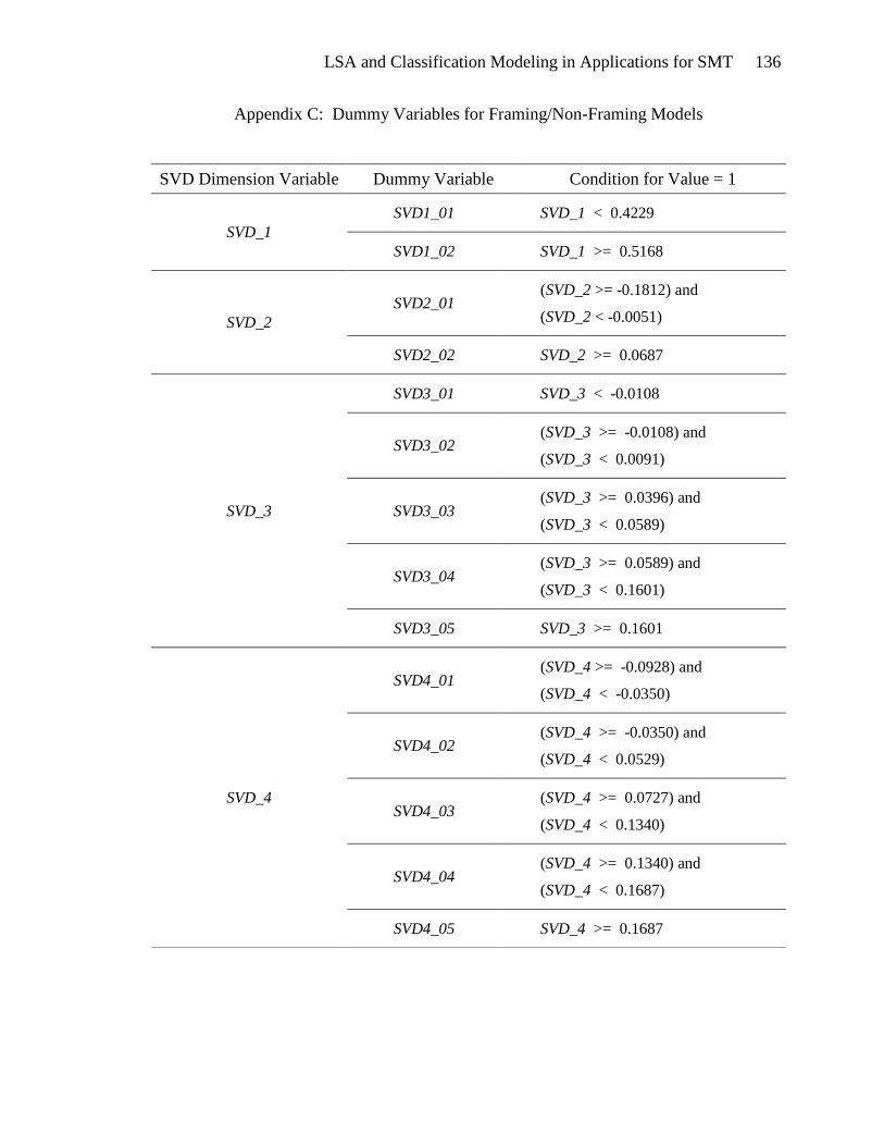
LSA and Classification Modeling in Applications for SMT 136
Appendix C: Dummy Variables for Framing/Non-Framing Models
SVD Dimension Variable Dummy Variable Condition for Value = 1
SVD_1
SVD1_01 SVD_1 < 0.4229
SVD1_02 SVD_1 >= 0.5168
SVD_2
SVD2_01 (SVD_2 >= -0.1812) and
(SVD_2 < -0.0051)
SVD2_02 SVD_2 >= 0.0687
SVD_3
SVD3_01 SVD_3 < -0.0108
SVD3_02 (SVD_3 >= -0.0108) and
(SVD_3 < 0.0091)
SVD3_03 (SVD_3 >= 0.0396) and
(SVD_3 < 0.0589)
SVD3_04 (SVD_3 >= 0.0589) and
(SVD_3 < 0.1601)
SVD3_05 SVD_3 >= 0.1601
SVD_4
SVD4_01 (SVD_4 >= -0.0928) and
(SVD_4 < -0.0350)
SVD4_02 (SVD_4 >= -0.0350) and
(SVD_4 < 0.0529)
SVD4_03 (SVD_4 >= 0.0727) and
(SVD_4 < 0.1340)
SVD4_04 (SVD_4 >= 0.1340) and
(SVD_4 < 0.1687)
SVD4_05 SVD_4 >= 0.1687
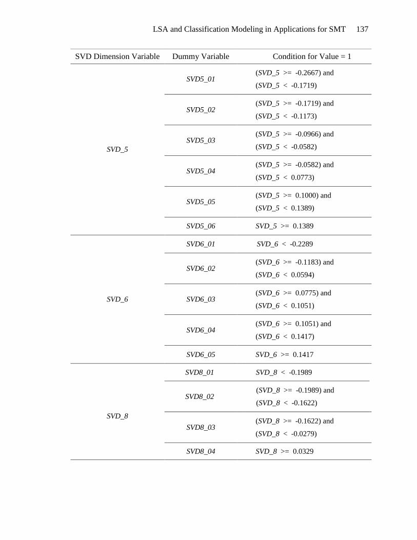
LSA and Classification Modeling in Applications for SMT 137
SVD Dimension Variable Dummy Variable Condition for Value = 1
SVD_5
SVD5_01 (SVD_5 >= -0.2667) and
(SVD_5 < -0.1719)
SVD5_02 (SVD_5 >= -0.1719) and
(SVD_5 < -0.1173)
SVD5_03 (SVD_5 >= -0.0966) and
(SVD_5 < -0.0582)
SVD5_04 (SVD_5 >= -0.0582) and
(SVD_5 < 0.0773)
SVD5_05 (SVD_5 >= 0.1000) and
(SVD_5 < 0.1389)
SVD5_06 SVD_5 >= 0.1389
SVD_6
SVD6_01 SVD_6 < -0.2289
SVD6_02 (SVD_6 >= -0.1183) and
(SVD_6 < 0.0594)
SVD6_03 (SVD_6 >= 0.0775) and
(SVD_6 < 0.1051)
SVD6_04 (SVD_6 >= 0.1051) and
(SVD_6 < 0.1417)
SVD6_05 SVD_6 >= 0.1417
SVD_8
SVD8_01 SVD_8 < -0.1989
SVD8_02 (SVD_8 >= -0.1989) and
(SVD_8 < -0.1622)
SVD8_03 (SVD_8 >= -0.1622) and
(SVD_8 < -0.0279)
SVD8_04 SVD_8 >= 0.0329
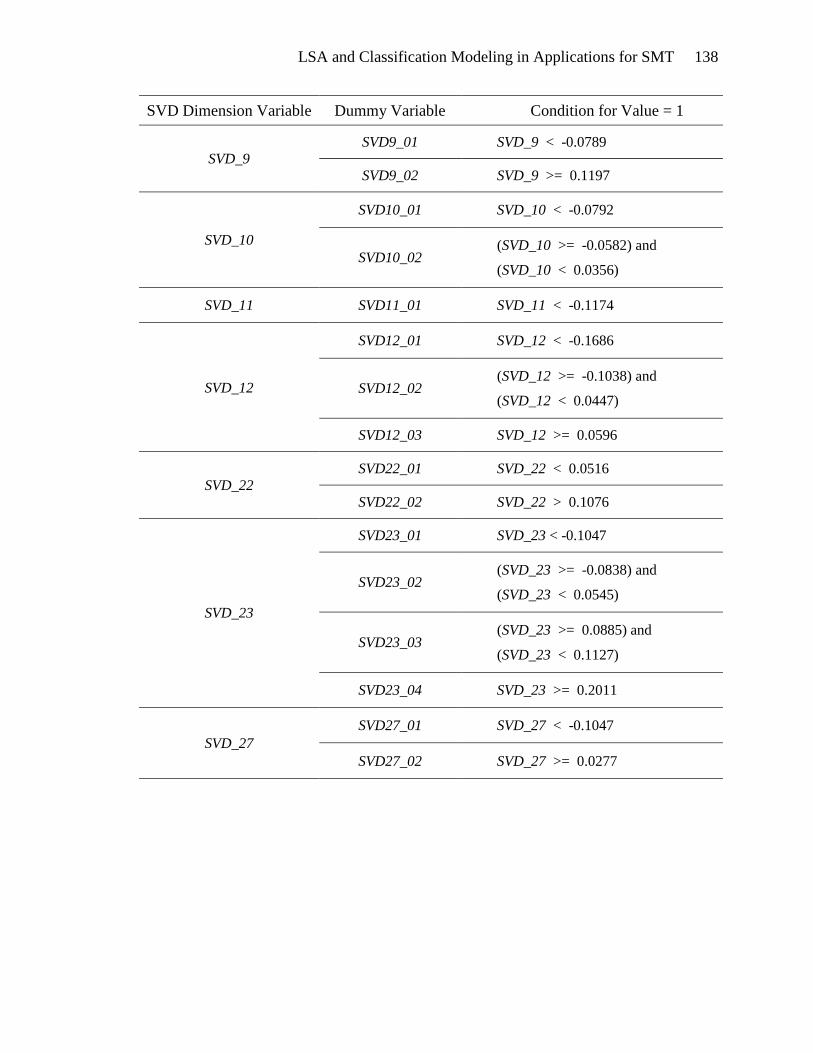
LSA and Classification Modeling in Applications for SMT 138
SVD Dimension Variable Dummy Variable Condition for Value = 1
SVD_9
SVD9_01 SVD_9 < -0.0789
SVD9_02 SVD_9 >= 0.1197
SVD_10
SVD10_01 SVD_10 < -0.0792
SVD10_02 (SVD_10 >= -0.0582) and
(SVD_10 < 0.0356)
SVD_11 SVD11_01 SVD_11 < -0.1174
SVD_12
SVD12_01 SVD_12 < -0.1686
SVD12_02 (SVD_12 >= -0.1038) and
(SVD_12 < 0.0447)
SVD12_03 SVD_12 >= 0.0596
SVD_22
SVD22_01 SVD_22 < 0.0516
SVD22_02 SVD_22 > 0.1076
SVD_23
SVD23_01 SVD_23 < -0.1047
SVD23_02 (SVD_23 >= -0.0838) and
(SVD_23 < 0.0545)
SVD23_03 (SVD_23 >= 0.0885) and
(SVD_23 < 0.1127)
SVD23_04 SVD_23 >= 0.2011
SVD_27
SVD27_01 SVD_27 < -0.1047
SVD27_02 SVD_27 >= 0.0277
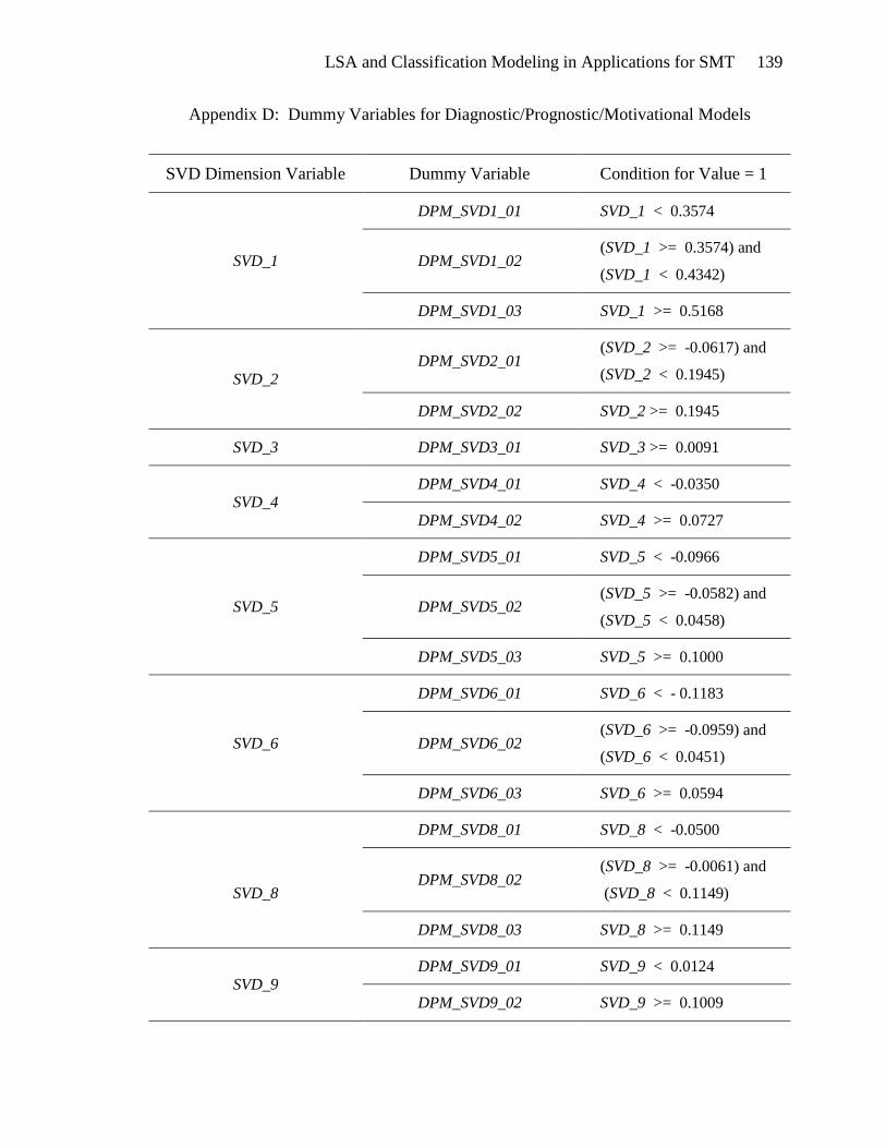
LSA and Classification Modeling in Applications for SMT 139
Appendix D: Dummy Variables for Diagnostic/Prognostic/Motivational Models
SVD Dimension Variable Dummy Variable Condition for Value = 1
SVD_1
DPM_SVD1_01 SVD_1 < 0.3574
DPM_SVD1_02 (SVD_1 >= 0.3574) and
(SVD_1 < 0.4342)
DPM_SVD1_03 SVD_1 >= 0.5168
SVD_2 DPM_SVD2_01
(SVD_2 >= -0.0617) and
(SVD_2 < 0.1945)
DPM_SVD2_02 SVD_2 >= 0.1945
SVD_3 DPM_SVD3_01 SVD_3 >= 0.0091
SVD_4
DPM_SVD4_01 SVD_4 < -0.0350
DPM_SVD4_02 SVD_4 >= 0.0727
SVD_5
DPM_SVD5_01 SVD_5 < -0.0966
DPM_SVD5_02 (SVD_5 >= -0.0582) and
(SVD_5 < 0.0458)
DPM_SVD5_03 SVD_5 >= 0.1000
SVD_6
DPM_SVD6_01 SVD_6 < - 0.1183
DPM_SVD6_02 (SVD_6 >= -0.0959) and
(SVD_6 < 0.0451)
DPM_SVD6_03 SVD_6 >= 0.0594
SVD_8
DPM_SVD8_01 SVD_8 < -0.0500
DPM_SVD8_02 (SVD_8 >= -0.0061) and
(SVD_8 < 0.1149)
DPM_SVD8_03 SVD_8 >= 0.1149
SVD_9 DPM_SVD9_01 SVD_9 < 0.0124
DPM_SVD9_02 SVD_9 >= 0.1009
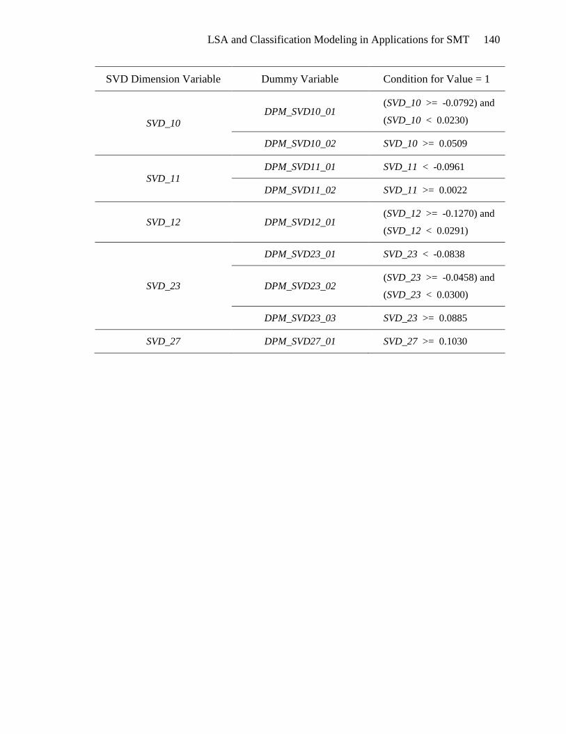
LSA and Classification Modeling in Applications for SMT 140
SVD Dimension Variable Dummy Variable Condition for Value = 1
SVD_10
DPM_SVD10_01 (SVD_10 >= -0.0792) and
(SVD_10 < 0.0230)
DPM_SVD10_02 SVD_10 >= 0.0509
SVD_11
DPM_SVD11_01 SVD_11 < -0.0961
DPM_SVD11_02 SVD_11 >= 0.0022
SVD_12 DPM_SVD12_01 (SVD_12 >= -0.1270) and
(SVD_12 < 0.0291)
SVD_23
DPM_SVD23_01 SVD_23 < -0.0838
DPM_SVD23_02 (SVD_23 >= -0.0458) and
(SVD_23 < 0.0300)
DPM_SVD23_03 SVD_23 >= 0.0885
SVD_27 DPM_SVD27_01 SVD_27 >= 0.1030
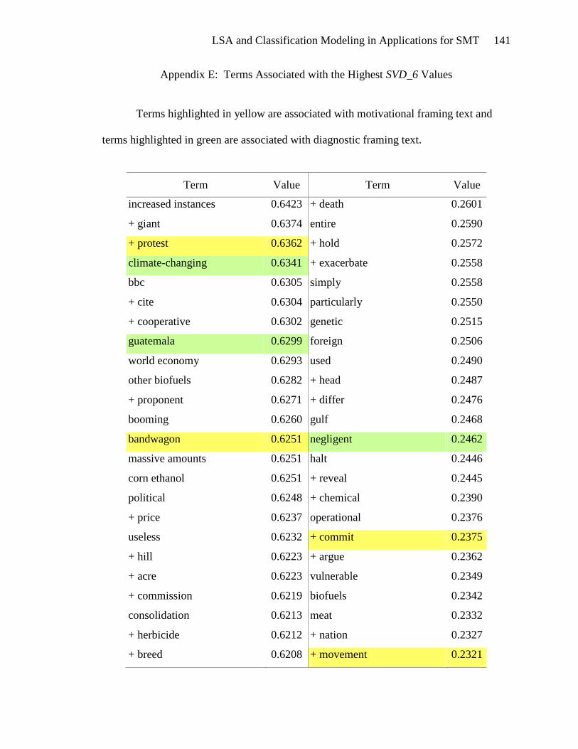
LSA and Classification Modeling in Applications for SMT 141
Appendix E: Terms Associated with the Highest SVD_6 Values
Terms highlighted in yellow are associated with motivational framing text and
terms highlighted in green are associated with diagnostic framing text.
Term Value Term Value
increased instances 0.6423 + death 0.2601
+ giant 0.6374 entire 0.2590
+ protest 0.6362 + hold 0.2572
climate-changing 0.6341 + exacerbate 0.2558
bbc 0.6305 simply 0.2558
+ cite 0.6304 particularly 0.2550
+ cooperative 0.6302 genetic 0.2515
guatemala 0.6299 foreign 0.2506
world economy 0.6293 used 0.2490
other biofuels 0.6282 + head 0.2487
+ proponent 0.6271 + differ 0.2476
booming 0.6260 gulf 0.2468
bandwagon 0.6251 negligent 0.2462
massive amounts 0.6251 halt 0.2446
corn ethanol 0.6251 + reveal 0.2445
political 0.6248 + chemical 0.2390
+ price 0.6237 operational 0.2376
useless 0.6232 + commit 0.2375
+ hill 0.6223 + argue 0.2362
+ acre 0.6223 vulnerable 0.2349
+ commission 0.6219 biofuels 0.2342
consolidation 0.6213 meat 0.2332
+ herbicide 0.6212 + nation 0.2327
+ breed 0.6208 + movement 0.2321
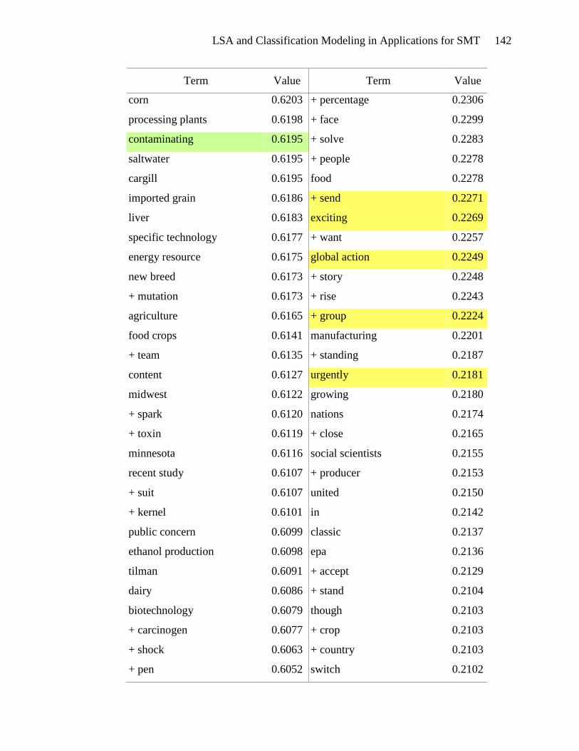
LSA and Classification Modeling in Applications for SMT 142
Term Value Term Value
corn 0.6203 + percentage 0.2306
processing plants 0.6198 + face 0.2299
contaminating 0.6195 + solve 0.2283
saltwater 0.6195 + people 0.2278
cargill 0.6195 food 0.2278
imported grain 0.6186 + send 0.2271
liver 0.6183 exciting 0.2269
specific technology 0.6177 + want 0.2257
energy resource 0.6175 global action 0.2249
new breed 0.6173 + story 0.2248
+ mutation 0.6173 + rise 0.2243
agriculture 0.6165 + group 0.2224
food crops 0.6141 manufacturing 0.2201
+ team 0.6135 + standing 0.2187
content 0.6127 urgently 0.2181
midwest 0.6122 growing 0.2180
+ spark 0.6120 nations 0.2174
+ toxin 0.6119 + close 0.2165
minnesota 0.6116 social scientists 0.2155
recent study 0.6107 + producer 0.2153
+ suit 0.6107 united 0.2150
+ kernel 0.6101 in 0.2142
public concern 0.6099 classic 0.2137
ethanol production 0.6098 epa 0.2136
tilman 0.6091 + accept 0.2129
dairy 0.6086 + stand 0.2104
biotechnology 0.6079 though 0.2103
+ carcinogen 0.6077 + crop 0.2103
+ shock 0.6063 + country 0.2103
+ pen 0.6052 switch 0.2102
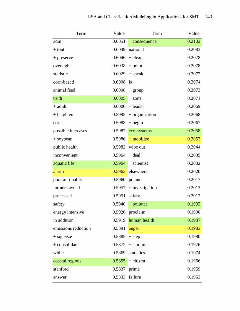
LSA and Classification Modeling in Applications for SMT 143
Term Value Term Value
adm. 0.6051 + consequence 0.2102
+ tout 0.6049 national 0.2083
+ preserve 0.6046 + clear 0.2078
oversight 0.6038 + point 0.2078
statistic 0.6029 + speak 0.2077
corn-based 0.6008 is 0.2074
animal feed 0.6008 + group 0.2073
truth 0.6005 + zone 0.2071
+ adult 0.6000 + leader 0.2069
+ heighten 0.5995 + organization 0.2068
corn 0.5988 + begin 0.2067
possible increases 0.5987 eco-systems 0.2058
+ soybean 0.5986 + mobilize 0.2053
public health 0.5982 wipe out 0.2044
inconvenient 0.5964 + deal 0.2035
aquatic life 0.5964 + scientist 0.2032
alarm 0.5963 elsewhere 0.2020
poor air quality 0.5960 poland 0.2017
farmer-owned 0.5957 + investigation 0.2013
processed 0.5951 safety 0.2012
safety 0.5940 + polluter 0.1992
energy intensive 0.5926 proclaim 0.1990
in addition 0.5919 human health 0.1987
emissions reduction 0.5891 anger 0.1983
+ squeeze 0.5885 + step 0.1980
+ consolidate 0.5872 + summit 0.1976
while 0.5869 statistics 0.1974
coastal regions 0.5855 + citizen 0.1966
stanford 0.5837 prime 0.1959
answer 0.5833 failure 0.1953
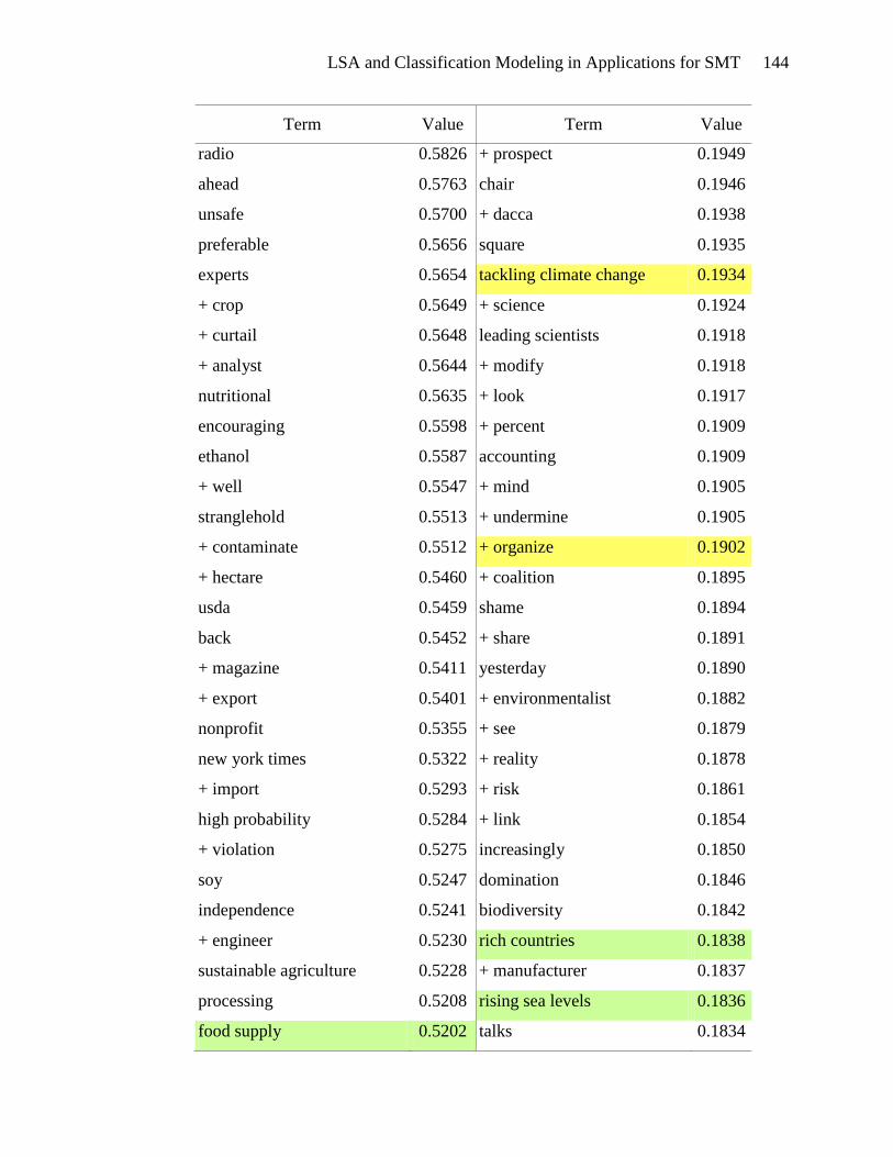
LSA and Classification Modeling in Applications for SMT 144
Term Value Term Value
radio 0.5826 + prospect 0.1949
ahead 0.5763 chair 0.1946
unsafe 0.5700 + dacca 0.1938
preferable 0.5656 square 0.1935
experts 0.5654 tackling climate change 0.1934
+ crop 0.5649 + science 0.1924
+ curtail 0.5648 leading scientists 0.1918
+ analyst 0.5644 + modify 0.1918
nutritional 0.5635 + look 0.1917
encouraging 0.5598 + percent 0.1909
ethanol 0.5587 accounting 0.1909
+ well 0.5547 + mind 0.1905
stranglehold 0.5513 + undermine 0.1905
+ contaminate 0.5512 + organize 0.1902
+ hectare 0.5460 + coalition 0.1895
usda 0.5459 shame 0.1894
back 0.5452 + share 0.1891
+ magazine 0.5411 yesterday 0.1890
+ export 0.5401 + environmentalist 0.1882
nonprofit 0.5355 + see 0.1879
new york times 0.5322 + reality 0.1878
+ import 0.5293 + risk 0.1861
high probability 0.5284 + link 0.1854
+ violation 0.5275 increasingly 0.1850
soy 0.5247 domination 0.1846
independence 0.5241 biodiversity 0.1842
+ engineer 0.5230 rich countries 0.1838
sustainable agriculture 0.5228 + manufacturer 0.1837
processing 0.5208 rising sea levels 0.1836
food supply 0.5202 talks 0.1834
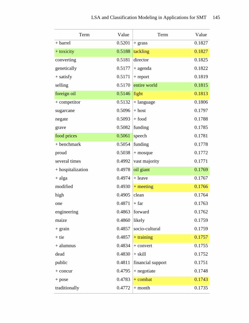
LSA and Classification Modeling in Applications for SMT 145
Term Value Term Value
+ barrel 0.5201 + grass 0.1827
+ toxicity 0.5188 tackling 0.1827
converting 0.5181 director 0.1825
genetically 0.5177 + agenda 0.1822
+ satisfy 0.5171 + report 0.1819
selling 0.5170 entire world 0.1815
foreign oil 0.5146 fight 0.1813
+ competitor 0.5132 + language 0.1806
sugarcane 0.5096 + host 0.1797
negate 0.5093 + food 0.1788
grave 0.5082 funding 0.1785
food prices 0.5061 speech 0.1781
+ benchmark 0.5054 funding 0.1778
proud 0.5038 + mosque 0.1772
several times 0.4992 vast majority 0.1771
+ hospitalization 0.4978 oil giant 0.1769
+ alga 0.4974 + leave 0.1767
modified 0.4930 + meeting 0.1766
high 0.4905 clean 0.1764
one 0.4871 + far 0.1763
engineering 0.4863 forward 0.1762
maize 0.4860 likely 0.1759
+ grain 0.4857 socio-cultural 0.1759
+ tie 0.4857 + training 0.1757
+ alumnus 0.4834 + convert 0.1755
dead 0.4830 + skill 0.1752
public 0.4811 financial support 0.1751
+ concur 0.4795 + negotiate 0.1748
+ pose 0.4783 + combat 0.1743
traditionally 0.4772 + month 0.1735
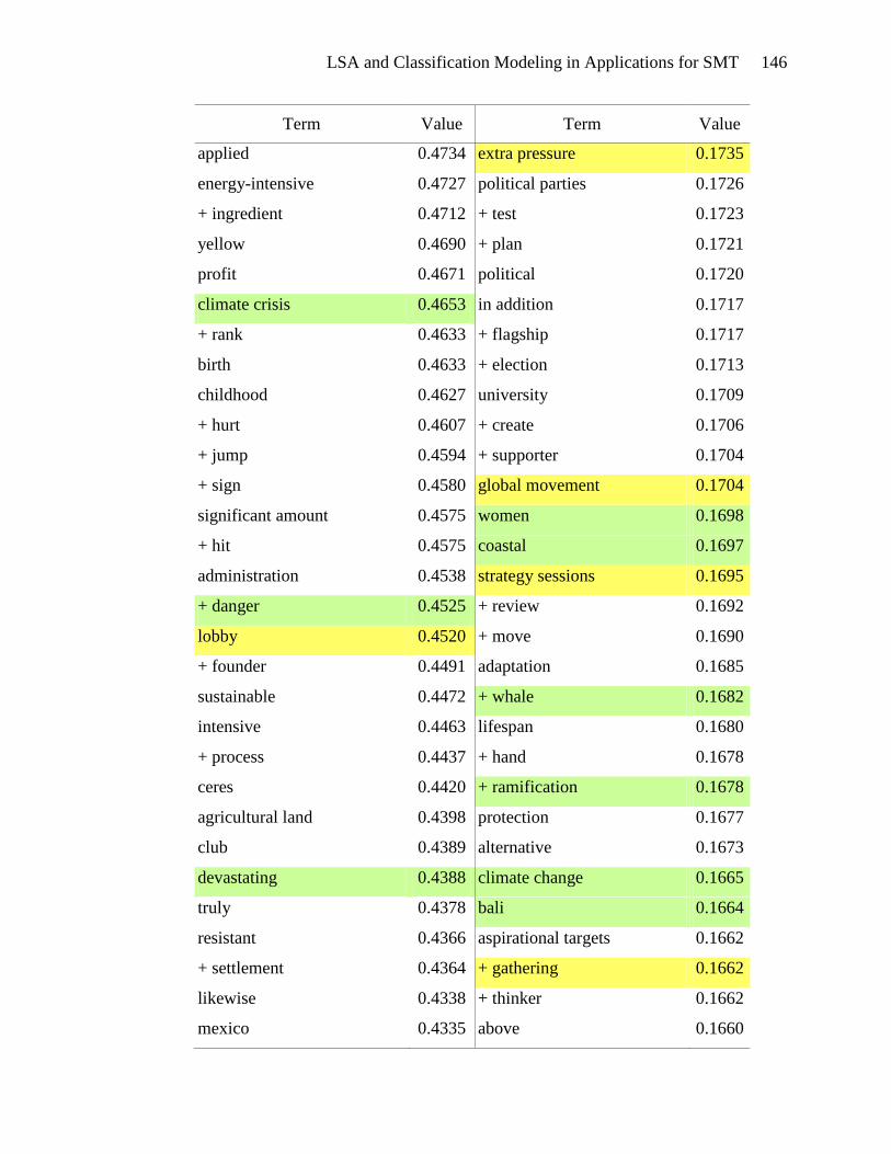
LSA and Classification Modeling in Applications for SMT 146
Term Value Term Value
applied 0.4734 extra pressure 0.1735
energy-intensive 0.4727 political parties 0.1726
+ ingredient 0.4712 + test 0.1723
yellow 0.4690 + plan 0.1721
profit 0.4671 political 0.1720
climate crisis 0.4653 in addition 0.1717
+ rank 0.4633 + flagship 0.1717
birth 0.4633 + election 0.1713
childhood 0.4627 university 0.1709
+ hurt 0.4607 + create 0.1706
+ jump 0.4594 + supporter 0.1704
+ sign 0.4580 global movement 0.1704
significant amount 0.4575 women 0.1698
+ hit 0.4575 coastal 0.1697
administration 0.4538 strategy sessions 0.1695
+ danger 0.4525 + review 0.1692
lobby 0.4520 + move 0.1690
+ founder 0.4491 adaptation 0.1685
sustainable 0.4472 + whale 0.1682
intensive 0.4463 lifespan 0.1680
+ process 0.4437 + hand 0.1678
ceres 0.4420 + ramification 0.1678
agricultural land 0.4398 protection 0.1677
club 0.4389 alternative 0.1673
devastating 0.4388 climate change 0.1665
truly 0.4378 bali 0.1664
resistant 0.4366 aspirational targets 0.1662
+ settlement 0.4364 + gathering 0.1662
likewise 0.4338 + thinker 0.1662
mexico 0.4335 above 0.1660
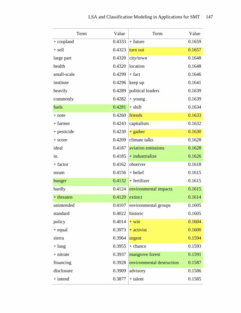
LSA and Classification Modeling in Applications for SMT 147
Term Value Term Value
+ cropland 0.4333 + future 0.1659
+ sell 0.4323 turn out 0.1657
large part 0.4320 city/town 0.1648
health 0.4320 location 0.1648
small-scale 0.4299 + fact 0.1646
institute 0.4296 keep up 0.1641
heavily 0.4289 political leaders 0.1639
commonly 0.4282 + young 0.1639
fuels 0.4281 + shift 0.1634
+ note 0.4260 friends 0.1633
+ farmer 0.4243 capitalism 0.1632
+ pesticide 0.4230 + gather 0.1630
+ score 0.4209 climate talks 0.1628
ideal 0.4187 aviation emissions 0.1628
in. 0.4185 + industrialize 0.1626
+ factor 0.4162 observer 0.1618
steam 0.4156 + belief 0.1615
hunger 0.4132 + fertilizer 0.1615
hardly 0.4124 environmental impacts 0.1615
+ threaten 0.4120 extinct 0.1614
unintended 0.4107 environmental groups 0.1605
standard 0.4022 historic 0.1605
policy 0.4014 + win 0.1604
+ equal 0.3973 + activist 0.1600
sierra 0.3964 urgent 0.1594
+ lung 0.3955 + chance 0.1593
+ nitrate 0.3937 mangrove forest 0.1591
financing 0.3928 environmental destruction 0.1587
disclosure 0.3909 advisory 0.1586
+ intend 0.3877 + talent 0.1585
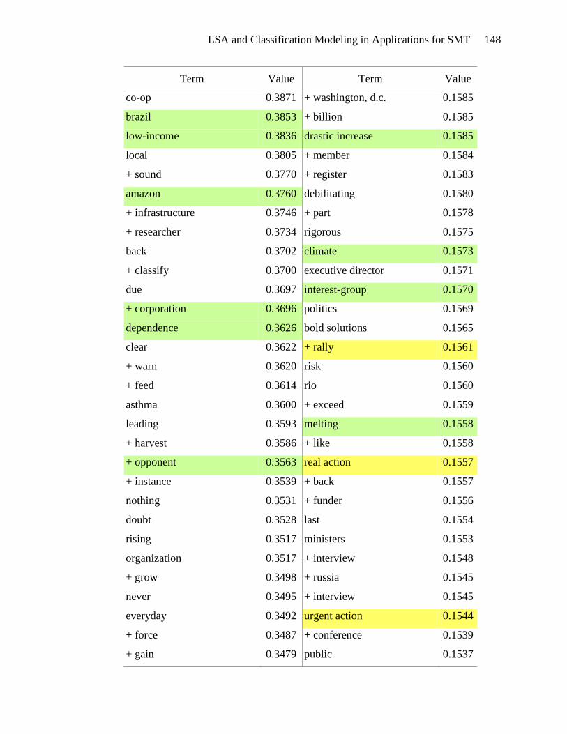
LSA and Classification Modeling in Applications for SMT 148
Term Value Term Value
co-op 0.3871 + washington, d.c. 0.1585
brazil 0.3853 + billion 0.1585
low-income 0.3836 drastic increase 0.1585
local 0.3805 + member 0.1584
+ sound 0.3770 + register 0.1583
amazon 0.3760 debilitating 0.1580
+ infrastructure 0.3746 + part 0.1578
+ researcher 0.3734 rigorous 0.1575
back 0.3702 climate 0.1573
+ classify 0.3700 executive director 0.1571
due 0.3697 interest-group 0.1570
+ corporation 0.3696 politics 0.1569
dependence 0.3626 bold solutions 0.1565
clear 0.3622 + rally 0.1561
+ warn 0.3620 risk 0.1560
+ feed 0.3614 rio 0.1560
asthma 0.3600 + exceed 0.1559
leading 0.3593 melting 0.1558
+ harvest 0.3586 + like 0.1558
+ opponent 0.3563 real action 0.1557
+ instance 0.3539 + back 0.1557
nothing 0.3531 + funder 0.1556
doubt 0.3528 last 0.1554
rising 0.3517 ministers 0.1553
organization 0.3517 + interview 0.1548
+ grow 0.3498 + russia 0.1545
never 0.3495 + interview 0.1545
everyday 0.3492 urgent action 0.1544
+ force 0.3487 + conference 0.1539
+ gain 0.3479 public 0.1537
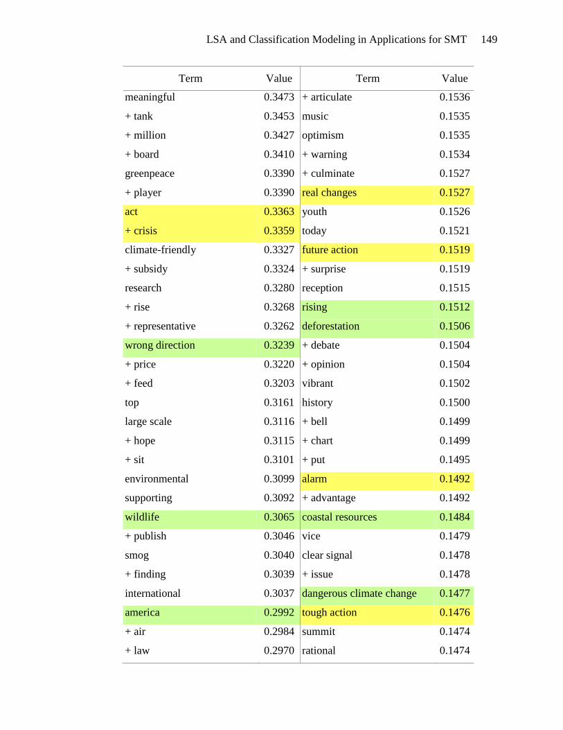
LSA and Classification Modeling in Applications for SMT 149
Term Value Term Value
meaningful 0.3473 + articulate 0.1536
+ tank 0.3453 music 0.1535
+ million 0.3427 optimism 0.1535
+ board 0.3410 + warning 0.1534
greenpeace 0.3390 + culminate 0.1527
+ player 0.3390 real changes 0.1527
act 0.3363 youth 0.1526
+ crisis 0.3359 today 0.1521
climate-friendly 0.3327 future action 0.1519
+ subsidy 0.3324 + surprise 0.1519
research 0.3280 reception 0.1515
+ rise 0.3268 rising 0.1512
+ representative 0.3262 deforestation 0.1506
wrong direction 0.3239 + debate 0.1504
+ price 0.3220 + opinion 0.1504
+ feed 0.3203 vibrant 0.1502
top 0.3161 history 0.1500
large scale 0.3116 + bell 0.1499
+ hope 0.3115 + chart 0.1499
+ sit 0.3101 + put 0.1495
environmental 0.3099 alarm 0.1492
supporting 0.3092 + advantage 0.1492
wildlife 0.3065 coastal resources 0.1484
+ publish 0.3046 vice 0.1479
smog 0.3040 clear signal 0.1478
+ finding 0.3039 + issue 0.1478
international 0.3037 dangerous climate change 0.1477
america 0.2992 tough action 0.1476
+ air 0.2984 summit 0.1474
+ law 0.2970 rational 0.1474
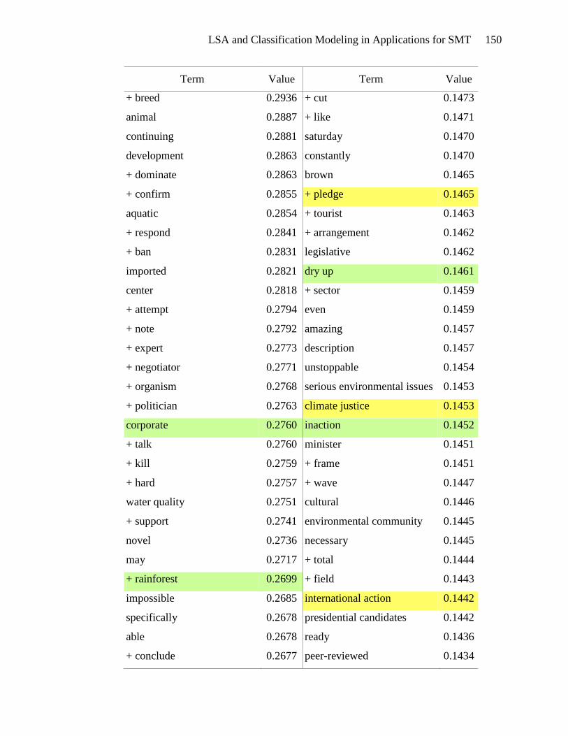
LSA and Classification Modeling in Applications for SMT 150
Term Value Term Value
+ breed 0.2936 + cut 0.1473
animal 0.2887 + like 0.1471
continuing 0.2881 saturday 0.1470
development 0.2863 constantly 0.1470
+ dominate 0.2863 brown 0.1465
+ confirm 0.2855 + pledge 0.1465
aquatic 0.2854 + tourist 0.1463
+ respond 0.2841 + arrangement 0.1462
+ ban 0.2831 legislative 0.1462
imported 0.2821 dry up 0.1461
center 0.2818 + sector 0.1459
+ attempt 0.2794 even 0.1459
+ note 0.2792 amazing 0.1457
+ expert 0.2773 description 0.1457
+ negotiator 0.2771 unstoppable 0.1454
+ organism 0.2768 serious environmental issues 0.1453
+ politician 0.2763 climate justice 0.1453
corporate 0.2760 inaction 0.1452
+ talk 0.2760 minister 0.1451
+ kill 0.2759 + frame 0.1451
+ hard 0.2757 + wave 0.1447
water quality 0.2751 cultural 0.1446
+ support 0.2741 environmental community 0.1445
novel 0.2736 necessary 0.1445
may 0.2717 + total 0.1444
+ rainforest 0.2699 + field 0.1443
impossible 0.2685 international action 0.1442
specifically 0.2678 presidential candidates 0.1442
able 0.2678 ready 0.1436
+ conclude 0.2677 peer-reviewed 0.1434
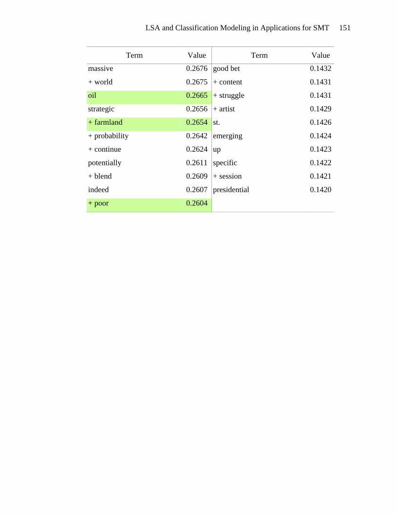
LSA and Classification Modeling in Applications for SMT 151
Term Value Term Value
massive 0.2676 good bet 0.1432
+ world 0.2675 + content 0.1431
oil 0.2665 + struggle 0.1431
strategic 0.2656 + artist 0.1429
+ farmland 0.2654 st. 0.1426
+ probability 0.2642 emerging 0.1424
+ continue 0.2624 up 0.1423
potentially 0.2611 specific 0.1422
+ blend 0.2609 + session 0.1421
indeed 0.2607 presidential 0.1420
+ poor 0.2604