Low-N protein engineering with data-efficient deep learning Surojit Biswas1†, Grigory Khimulya 3†, Ethan C. Alley2†, Kevin M. Esvelt2, George M. Church 1,4 1 Wyss Institute for Biologically Inspired Engineering, Harvard University 2 MIT Media Lab, Massachusetts Institute of Technology 3 Somerville, MA 02143, USA 4 Department of Genetics, Harvard Medical School

†These authors contributed equally to this work. *Correspondence to: George M. Church: gchurch{at}genetics.med.harvard.edu

Abstract Protein engineering has enormous academic and industrial potential. However, it is limited by the lack of experimental assays that are consistent with the design goal and sufficiently high-throughput to find rare, enhanced variants. Here we introduce a machine learning-guided paradigm that can use as few as 24 functionally assayed mutant sequences to build an accurate virtual fitness landscape and screen ten million sequences via in silico directed evolution. As demonstrated in two highly dissimilar proteins, avGFP and TEM-1 β -lactamase, top candidates from a single round are diverse and as active as engineered mutants obtained from previous multi-year, high-throughput efforts. Because it distills information from both global and local sequence landscapes, our model approximates protein function even before receiving experimental data, and generalizes from only single mutations to propose high-functioning epistatically non-trivial designs. With reproducible >500% improvements in activity from a single assay in a 96-well plate, we demonstrate the strongest generalization observed in machine-learning guided protein design to date. Taken together, our approach enables efficient use of resource intensive high-fidelity assays without sacrificing throughput. By encouraging alignment with endpoint objectives, low-N design will accelerate engineered proteins into the fermenter, field, and clinic.

1

.CC-BY-NC-ND 4.0 International license(which was not certified by peer review) is the author/funder. It is made available under aThe copyright holder for this preprintthis version posted January 24, 2020. . https://doi.org/10.1101/2020.01.23.917682doi: bioRxiv preprint

Introduction Protein engineering holds great promise for nanotechnology, agriculture, and medicine. However, design is limited by our ability to search through the vastness of protein sequence space, which is only sparsely functional 1,2. When searching for high functioning sequences, engineers must be wary of the pervasive maxim, “you get what you screen for”, which cautions against over-optimizing a protein’s sequence using functional assays that may not be fully aligned with the final design objective 3–6. However, in most resource-constrained real-world settings, including the design of protein therapeutics7,8, agricultural proteins9, and industrial biocatalysts10,11, engineers must often compromise assay fidelity (careful endpoint-resembling measurements of a small number of variants) for assay throughput (high-throughput proxy measurements for a large number of variants)12,13. Consequently, the best candidates identified by early stage high-throughput (>10 4 variants) proxy experiments9,11,14 will often fail in validation under higher-fidelity, later stage assays13,15–17. Moreover, high-throughput assays do not exist at all for many classes of proteins, making them inaccessible to screening and directed evolution 18–24. Here we focus on enabling large-scale exploration of sequence space using only a small number — “low-N” — of functionally characterized training variants. We recently developed UniRep 25, a deep learning model trained on a large unlabeled protein sequence dataset. From scratch and from sequence alone, UniRep learned to distill the fundamental features of a protein — including biophysical, structural, and evolutionary information — into a holistic statistical summary, or representation . We reasoned that combining UniRep’s global knowledge of functional proteins with just a few dozen functionally characterized mutants of the target protein might suffice to build a high-quality model of a protein’s fitness landscape. Combined with in silico directed evolution, we hypothesized that we could computationally explore these landscapes at a scale of 10 7-10 8 variants, rivalling even the highest-throughput screens. Here, we test this paradigm in two fundamentally different proteins — a eukaryotic green fluorescent protein from Aequorea victoria (avGFP), and a prokaryotic β -lactam hydrolyzing enzyme from Escherichia coli (TEM-1 β -lactamase). We demonstrate reliable production of substantially optimized designs with just 24 or 96 characterized sequence variants as training data.

Results

A paradigm for low-N protein engineering To meet the enormous data requirement of supervised deep learning — typically greater than 10 6 labeled data points26,27— current machine learning-guided protein design approaches must gather high-throughput experimental data 28–31 or abandon deep learning altogether18,20,21,32–37. We reasoned that UniRep could leverage its existing knowledge of functional protein sequences to substantially reduce this prohibitive data requirement and enable low-N design. For low-N engineering of a given target protein, our approach features five steps:

2

.CC-BY-NC-ND 4.0 International license(which was not certified by peer review) is the author/funder. It is made available under aThe copyright holder for this preprintthis version posted January 24, 2020. . https://doi.org/10.1101/2020.01.23.917682doi: bioRxiv preprint

1) Global unsupervised pre-training of UniRep on >20 million raw amino acid sequences to distill general features of all functional proteins, as described previously25.

2) Unsupervised fine-tuning of UniRep on sequences evolutionarily related to the target protein (evotuning) to learn the distinct features of the target family. We call this model, which combines features from both the global and local sequence landscape, evotuned UniRep, or eUniRep.

3) Functional characterization of a low-N number of random mutants of the wild-type target protein to train a simple supervised top model that uses eUniRep’s representation as input (Fig. 1c). Together, eUnirep and the top model define an end-to-end sequence-to-function model that serves as a surrogate of the protein’s fitness landscape.

4) Markov Chain Monte Carlo-based in silico directed evolution on this surrogate landscape (Fig. 1d-e). 5) Experimental characterization of top sequence candidates that are predicted to have improved function

relative to wild-type (>WT). To understand the utility of eUniRep’s global + local representation, we considered a control model which was trained de novo solely on the local sequence neighborhood 38–41 of the target protein (Local UniRep). Thus, Local UniRep lacks global information about all known sequence space. As an additional control, we included one-hot encoding, as an explicit and exact flattened binary matrix representation of the full amino acid sequence (Full AA), to contextualize the importance of any evolutionary information (Methods). We first evaluated our approach in retrospective experiments using pre-existing and newly designed datasets of characterized mutant proteins (Methods, Supplementary Fig. 1). We found that only globally pre-trained eUniRep enabled consistent low-N retrospective performance, and that with the right regularized top model, meaningful generalization required only 24 training mutants (Supplementary Fig. 2). Random selection of these 24 mutants from the output of error-prone PCR or single-mutation deep mutational scans worked as well as more tailored approaches (Methods).

3

.CC-BY-NC-ND 4.0 International license(which was not certified by peer review) is the author/funder. It is made available under aThe copyright holder for this preprintthis version posted January 24, 2020. . https://doi.org/10.1101/2020.01.23.917682doi: bioRxiv preprint

Figure 1. UniRep-guided in silico directed evolution for low-N protein engineering. a) UniRep is globally trained on a large sequence database (UniRef50) as described previously25. b) This trained, unsupervised model is further fine-tuned to sequences that are evolutionarily related to the protein of engineering interest (eUniRep). c) A low-N number of mutants are obtained, characterized, and used to train regularized linear regression “on top” of eUniRep’s representation. d) In silico directed evolution is used to navigate this virtual fitness landscape and propose putatively optimized designs that are then experimentally characterized. This design loop may be repeated until desired functionality is reached. e) Illustration of the evolutionary process.

Low-N engineering of the fluorescent protein avGFP To test our approach prospectively, we attempted low-N optimization of the fluorescence intensity of the original green fluorescent protein from Aequorea victoria (avGFP) (Fig. 2a). The design process consisted of randomly sampling N=24 or N=96 training mutants from error-prone PCR42, representing sequences, training a top model, and performing in silico directed evolution to produce 300 putatively optimized designs within a 15 mutation “trust radius” of wild-type (Methods). We replicated this process 5 times for each combination of tested variables, yielding a total of 12,800 sequence designs. The design window spanned a functionally relevant 81 amino acid region of avGFP that included the central chromophore-bearing helix and four straddling beta-sheets (Fig. 2a; Methods; Supplementary Fig. 3). Evotuning globally pre-trained UniRep was reproducible, and in 19 out of 20 replicates (95%), eUniRep enabled a 10 +/- 2% (95% CI) hit rate, defined as designs with activity greater than wild-type (eUniRep 1 & 2; Fig. 2b). Constraining in silico evolution to a 7 mutation trust radius improved eUniRep’s hit rate to 18% without loss of quantitative fluorescence (Supplementary Fig. 4). Based on these numbers, “24-to-24 design” appeared

4

.CC-BY-NC-ND 4.0 International license(which was not certified by peer review) is the author/funder. It is made available under aThe copyright holder for this preprintthis version posted January 24, 2020. . https://doi.org/10.1101/2020.01.23.917682doi: bioRxiv preprint

tractable, where the characterization of just 24 training mutants and 24 optimized designs would be sufficient to observe a >WT design 1.8 +/- 0.8 (95% CI) times (Supplementary Fig. 5). By contrast, prospective design on Full AA or Local UniRep was inconsistent and only enabled ~0% and ~2% hit rates, respectively. We clonally validated our best designs and compared them to sequences produced by ancestral sequence reconstruction (ASR)43,44 and consensus sequence design 45,46 (Methods). While both consistently provided >WT variants, eUniRep designs were substantially more functional (Fig. 2c). Several, in fact, were on par with superfolder GFP (sfGFP; Fig. 2c), which is the result of a multi-year engineering effort that started with avGFP and benefits from mutations outside of our design window. Importantly, eUniRep designs were diverse and occupied a unique region of sequence space, different from extant, ASR, and consensus sequences (median minimum number of mutations = 5, Fig. 2d).

5

.CC-BY-NC-ND 4.0 International license(which was not certified by peer review) is the author/funder. It is made available under aThe copyright holder for this preprintthis version posted January 24, 2020. . https://doi.org/10.1101/2020.01.23.917682doi: bioRxiv preprint

Figure 2. eUniRep enables low-N engineering of avGFP . a) Experimental workflow describing training mutant acquisition, sequence-to-function modeling, in silico directed evolution, and the use of FlowSeq to quantitatively characterize designs in multiplex. b) Low-N engineering results for 24 (top) and 96 (bottom) training mutants. eUniRep 1 and 2 correspond to two replicate evotunings initialized from the same globally pre-trained UniRep. c) Quantitative flow-cytometric measurements of top eUniRep and Local UniRep designs, as well as ASR and consensus sequence designs. Shown above are false-colored images of E. coli expressing avGFP (av), sfGFP (sf), and a subset of the designs under 405 nm or 488 nm excitation, read with a 525/50 emission filter. d) Distance-preserving multidimensional scaling plot illustrating the diversity of eUniRep designs compared to existing GFPs, ASRs, and consensus sequence designs. Scale bar of 2 mutations shown.

Low-N engineering of the enzyme TEM-1 β-lactamase We next challenged our approach to generalize to the enzyme TEM-1 β -lactamase and optimize protein function training only on single mutants, which lack epistatic information 47. Not only is this an arduous task due to the essential role of epistasis in proteins48,49, but also TEM-1 β -lactamase is dissimilar to avGFP both

6

.CC-BY-NC-ND 4.0 International license(which was not certified by peer review) is the author/funder. It is made available under aThe copyright holder for this preprintthis version posted January 24, 2020. . https://doi.org/10.1101/2020.01.23.917682doi: bioRxiv preprint

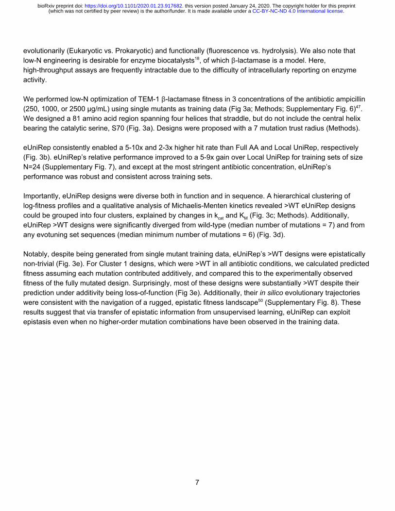
evolutionarily (Eukaryotic vs. Prokaryotic) and functionally (fluorescence vs. hydrolysis). We also note that low-N engineering is desirable for enzyme biocatalysts18, of which β -lactamase is a model. Here, high-throughput assays are frequently intractable due to the difficulty of intracellularly reporting on enzyme activity. We performed low-N optimization of TEM-1 β -lactamase fitness in 3 concentrations of the antibiotic ampicillin (250, 1000, or 2500 μg/mL ) using single mutants as training data (Fig 3a; Methods; Supplementary Fig. 6)47. We designed a 81 amino acid region spanning four helices that straddle, but do not include the central helix bearing the catalytic serine, S70 (Fig. 3a). Designs were proposed with a 7 mutation trust radius (Methods). eUniRep consistently enabled a 5-10x and 2-3x higher hit rate than Full AA and Local UniRep, respectively (Fig. 3b). eUniRep’s relative performance improved to a 5-9x gain over Local UniRep for training sets of size N=24 (Supplementary Fig. 7), and except at the most stringent antibiotic concentration, eUniRep’s performance was robust and consistent across training sets. Importantly, eUniRep designs were diverse both in function and in sequence. A hierarchical clustering of log-fitness profiles and a qualitative analysis of Michaelis-Menten kinetics revealed >WT eUniRep designs could be grouped into four clusters, explained by changes in kcat and KM (Fig. 3c; Methods). Additionally, eUniRep >WT designs were significantly diverged from wild-type (median number of mutations = 7) and from any evotuning set sequences (median minimum number of mutations = 6) (Fig. 3d). Notably, despite being generated from single mutant training data, eUniRep’s >WT designs were epistatically non-trivial (Fig. 3e). For Cluster 1 designs, which were >WT in all antibiotic conditions, we calculated predicted fitness assuming each mutation contributed additively, and compared this to the experimentally observed fitness of the fully mutated design. Surprisingly, most of these designs were substantially >WT despite their prediction under additivity being loss-of-function (Fig 3e). Additionally, their in silico evolutionary trajectories were consistent with the navigation of a rugged, epistatic fitness landscape 50 (Supplementary Fig. 8). These results suggest that via transfer of epistatic information from unsupervised learning, eUniRep can exploit epistasis even when no higher-order mutation combinations have been observed in the training data.

7

.CC-BY-NC-ND 4.0 International license(which was not certified by peer review) is the author/funder. It is made available under aThe copyright holder for this preprintthis version posted January 24, 2020. . https://doi.org/10.1101/2020.01.23.917682doi: bioRxiv preprint

Figure 3. eUniRep enables low-N engineering of the enzyme TEM-1 β-lactamase using only single mutants as training data. a) Experimental workflow describing training mutant acquisition, sequence-to-function modeling, in silico directed evolution, and plate-based antibiotic selection combined with NGS sequencing to characterize designs. b) Low-N engineering results using N=96 training mutants for three different antibiotic selections. c) Heatmap illustrating log10(fitness) of all >WT eUniRep designs. Four clusters are annotated, and for each, likely changes to kcat and K M

-1 relative to wild-type are qualitatively shown. d) Bar plots illustrating the number of mutations of eUniRep designs to WT (left), and to the nearest member of the evotuning sequence set (right). e) Scatter plot of eUniRep Cluster 1 (highly >WT) designs illustrating observed fold change in fitness (relative to wild-type) vs predicted fold change in fitness under additivity.

8

.CC-BY-NC-ND 4.0 International license(which was not certified by peer review) is the author/funder. It is made available under aThe copyright holder for this preprintthis version posted January 24, 2020. . https://doi.org/10.1101/2020.01.23.917682doi: bioRxiv preprint

eUniRep’s first principal component naturally correlates with protein function We next attempted to explain eUniRep’s unique ability to enable low-N engineering (Fig. 4, Supplementary Fig. 9-11). While mutations in eUniRep proposals and >WT designs were biased toward solvent-exposed residues, a substantial fraction (40% GFP and 28% β -lactamase) were targeted to buried positions including the avGFP chromophore (Fig. 4a, Supplementary Fig. 9). This suggested that eUniRep could make non-trivial, beneficial rearrangements to the hydrophobic core, which previous work has suggested is difficult29. Additionally, we observed that the most functional β -lactamase designs were not preferentially mutated near the catalytic serine (S70), which ran counter to the typical engineering heuristic of targeting mutations to an enzyme’s active site 19. This result also suggested eUniRep can exploit non-local epistatic interactions (Fig. 4b, Supplementary Fig. 9). Unsurprisingly, eUniRep’s mutational preference could not be explained by first-order position-wise mutational tolerance, suggesting that eUniRep enabled more than consensus sequence design despite both methods drawing on evolutionary information (Fig. 2c, Supplementary Fig. 10). Not finding a clear explanation for eUniRep’s performance among these structural and evolutionary analyses, we examined the eUniRep sequence representation. Strikingly, we found a strong correlation between its primary axis of variation (principal component 1; PC1) and protein function (Fig. 4c-d; avGFP Pearson r = 0.51, 0.52; β -lactamase Pearson r = 0.44), which was not observed for PC1 of the Full AA representation (avGFP Pearson r = 0.02, β -lactamase Pearson r = 0.05). eUniRep was not provided with explicit information about protein function during training, and therefore learned to approximate it as the axis of greatest variance de novo . We hypothesize this may be a natural, but unexpected consequence of being forced to distill a semantic representation from raw sequence, to an extent that function itself provides a compelling summary of the local and global sequence landscape. This framing not only provides a plausible explanation for eUniRep’s low-N design success, but also suggests even lower-N design may be possible if training mutants are chosen to maximize variation in eUniRep’s PC1.

9

.CC-BY-NC-ND 4.0 International license(which was not certified by peer review) is the author/funder. It is made available under aThe copyright holder for this preprintthis version posted January 24, 2020. . https://doi.org/10.1101/2020.01.23.917682doi: bioRxiv preprint

Figure 4. eUniRep designs are structurally non-trivial and explained by unsupervised distillation of protein function. a) Structural visualization of avGFP (PDB: 2WUR). Mutations colored by relative frequency in >WT designs. Top 3 residues by mutation count shown as sticks. Chromophore colored by count of mutations made to any of the chromophore residues. b) As in a) but for the TEM-1 β -lactamase structure (PDB: 1ZG4), where the catalytic serine (S70) is highlighted in red. c) PCA of Full AA and eUniRep representations of sequences from the local fitness landscape of avGFP, colored by log10(relative fluorescence). Below each plot, log 10(relative fluorescence) as a function of PC1, Pearson r = 0.02 (Full AA), r = 0.52 (eUniRep 1), r = 0.51 (eUniRep 2). Cyan and magenta lines show two example in silico evolution trajectories in the principal component space. d) As in c), but for TEM-1 β -lactamase, where only one evotuning replicate was run (Methods). Points are colored by fitness. Below each plot, fitness as a function of PC1 (Full AA Pearson r = -0.05, eUniRep r = 0.44).

Discussion This work is the first to demonstrate a generalizable and scalable paradigm for low-N protein engineering. By distilling information from both the global and local sequence landscape, we reproducibly leveraged N=24 random training mutants and one round of in silico screening into over 1000 novel >WT designs. This is the strongest case of generalization- and data-efficiency in machine learning guided protein design to date (Supplementary Fig. 12). We took advantage of robust, high-fidelity multiplexed assays to extensively characterize our approach on avGFP and TEM-1 β -lactamase. While low-N design is intended for proteins where such assays are not available, both proteins have a rich history of being studied or engineered with them. As such, we consider existing >WT variants to be a high bar. Here, with just 24 random mutants of avGFP as training data, we

10

.CC-BY-NC-ND 4.0 International license(which was not certified by peer review) is the author/funder. It is made available under aThe copyright holder for this preprintthis version posted January 24, 2020. . https://doi.org/10.1101/2020.01.23.917682doi: bioRxiv preprint

designed novel FPs that rivaled sfGFP, the product of many years of high-throughput, high-fidelity protein engineering. Nevertheless, unlike GFP and TEM-1 β -lactamase, most proteins do not have assays that are both high-throughput and high-fidelity. In many therapeutic and industrial projects, high-fidelity experimental measurements of endpoint functions, like crop yield or biologic efficacy, are scarce and come at the end of long test cycles. In theory, generating high-throughput proxy assays of these endpoints should improve engineering success rates. However, empirically this is often not the case as evidenced, for example, by Eroom’s law in drug development13,15. Here efforts to use high-throughput proxy assays for the endpoint in question may in fact generate worse candidates for later-stage development13,15 by over-optimizing a biased metric51. Taken together, this suggests generalizing from low-N high-fidelity measurements may be more important than learning from high-N low-fidelity measurements. Indeed, several previous efforts successfully engineered valuable proteins using high-fidelity assays and low-N design 19,23,24,52–56. However, these (semi-)rational protein engineering approaches intensively rely on hand-crafted structural or (co)-evolutionary priors to narrow the search space of potential mutations8,19,57,58. Additionally, they often require expert judgment to learn from data, which may include modifying energy functions for biophysical design 59, and iteratively designing and testing structure-guided mutation combinations19,60–62. Together these modeling and design choices introduce biases that could manifest as a mismatch between optimization metric and endpoint. By contrast, UniRep and our low-N approach are paradigmatically empirical and sequence-based, improving with the exponential growth of sequence databases25 to minimize bias, and leaving open the possibility of discovering new principles of protein folding and activity that extend beyond our current mental models. Indeed, when combining data-driven digital fitness landscapes with in silico evolution to both measure well and search far, we find there may be surprising diversity and function in the vastness of sequence space. Acknowledgements: We thank Mohammed AlQuraishi, Chris Bakerlee, Anush Chiappino-Pepe, Aleksandra Eremina, Kyle Fish, Sager Gosai, Xiaoge Guo, Eric Kelsic, Pierce Ogden, Sam Sinai, Max Schubert, Amaro Taylor-Weiner, David Thompson, and Aaron Tucker for feedback on earlier drafts of this manuscript. We thank members of the Esvelt and Church labs for valuable discussion. S.B. was supported by an NSF GRFP Fellowship under grant number DGE1745303. G.K. was supported by a grant from the Center for Effective Altruism. E.C.A. was supported by a scholarship from the Open Philanthropy Project. This material is based upon work supported by the U.S. Department of Energy, Office of Science under Award Number DE-FG02-02ER63445. Computational resources were, in part, generously provided by the AWS Cloud Credits for Research Program. Author contributions: S.B., G.K., E.C.A. conceived the study. S.B. performed wet-lab experiments and managed data. S.B., G.K., E.C.A. performed machine learning modeling and data analyses. K.E. and G.M.C. supervised the project. S.B., G.K., E.C.A. wrote the manuscript with help from all authors. Competing interests: A full list of G.M.C.’s tech transfer, advisory roles, and funding sources can be found on the lab’s website: http://arep.med.harvard.edu/gmc/tech.html

11

.CC-BY-NC-ND 4.0 International license(which was not certified by peer review) is the author/funder. It is made available under aThe copyright holder for this preprintthis version posted January 24, 2020. . https://doi.org/10.1101/2020.01.23.917682doi: bioRxiv preprint

Code availability: Code for UniRep model training and inference with trained weights along with links to all necessary data is available at https://github.com/churchlab/UniRep .

References

1. Romero, P. A. & Arnold, F. H. Exploring protein fitness landscapes by directed evolution. Nat. Rev. Mol. Cell Biol. 10 , 866–876 (2009).

2. Packer, M. S. & Liu, D. R. Methods for the directed evolution of proteins. Nat. Rev. Genet. 16 , 379–394 (2015).

3. Lutz, S. & Patrick, W. M. Novel methods for directed evolution of enzymes: quality, not quantity. Curr. Opin. Biotechnol. (2004).

4. Goldsmith, M. & Tawfik, D. S. Directed enzyme evolution: beyond the low-hanging fruit. Curr. Opin. Struct. Biol. (2012).

5. Zhao, H. & Arnold, F. H. Combinatorial protein design: strategies for screening protein libraries. Curr. Opin. Struct. Biol. 7 , 480–485 (1997).

6. You, L. & Arnold, F. H. Directed evolution of subtilisin E in Bacillus subtilis to enhance total activity in aqueous dimethylformamide. Protein Eng. 9 , 77–83 (1996).

7. Lagassé, H. A. D. et al. Recent advances in (therapeutic protein) drug development. F1000Res. 6 , 113 (2017).

8. Marshall, S. A., Lazar, G. A., Chirino, A. J. & Desjarlais, J. R. Rational design and engineering of therapeutic proteins. Drug Discov. Today 8 , 212–221 (2003).

9. Rao, A. G. The outlook for protein engineering in crop improvement. Plant Physiol. 147 , 6–12 (2008). 10. Schmid, A. et al. Industrial biocatalysis today and tomorrow. Nature 409 , 258–268 (2001). 11. Sheldon, R. A. & Pereira, P. C. Biocatalysis engineering: the big picture. Chem. Soc. Rev. 46 , 2678–2691

(2017). 12. Mullard, A. Better screening and disease models needed. Nat. Rev. Drug Discov. 15 , 151–151 (2016). 13. Scannell, J. W. & Bosley, J. When Quality Beats Quantity: Decision Theory, Drug Discovery, and the

Reproducibility Crisis. PLoS One 11 , e0147215 (2016). 14. Hughes, J. P., Rees, S., Kalindjian, S. B. & Philpott, K. L. Principles of early drug discovery. Br. J.

Pharmacol. 162 , 1239–1249 (2011). 15. Scannell, J. W., Blanckley, A., Boldon, H. & Warrington, B. Diagnosing the decline in pharmaceutical R&D

efficiency. Nat. Rev. Drug Discov. 11 , 191–200 (2012). 16. Laverty, H. et al. How can we improve our understanding of cardiovascular safety liabilities to develop

safer medicines? Br. J. Pharmacol. 163 , 675–693 (2011). 17. Silver, L. L. Challenges of antibacterial discovery. Clin. Microbiol. Rev. 24 , 71–109 (2011). 18. Wu, Z., Jennifer Kan, S. B., Lewis, R. D., Wittmann, B. J. & Arnold, F. H. Machine learning-assisted

directed protein evolution with combinatorial libraries. Proceedings of the National Academy of Sciences vol. 116 8852–8858 (2019).

19. Lutz, S. Beyond directed evolution—semi-rational protein engineering and design. Curr. Opin. Biotechnol. (2010).

20. Bedbrook, C. N., Yang, K. K., Rice, A. J., Gradinaru, V. & Arnold, F. H. Machine learning to design integral membrane channelrhodopsins for efficient eukaryotic expression and plasma membrane localization. PLoS Comput. Biol. 13 , e1005786 (2017).

21. Bedbrook, C. N. et al. Machine learning-guided channelrhodopsin engineering enables minimally invasive optogenetics. Nat. Methods 16 , 1176–1184 (2019).

12

.CC-BY-NC-ND 4.0 International license(which was not certified by peer review) is the author/funder. It is made available under aThe copyright holder for this preprintthis version posted January 24, 2020. . https://doi.org/10.1101/2020.01.23.917682doi: bioRxiv preprint

22. Romney, D. K., Murciano-Calles, J., Wehrmüller, J. E. & Arnold, F. H. Unlocking Reactivity of TrpB: A General Biocatalytic Platform for Synthesis of Tryptophan Analogues. J. Am. Chem. Soc. 139 , 10769–10776 (2017).

23. Silva, D. A., Yu, S., Ulge, U. Y., Spangler, J. B. & Jude, K. M. De novo design of potent and selective mimics of IL-2 and IL-15. Nature (2019).

24. Marcandalli, J., Fiala, B., Ols, S. & Perotti, M. Induction of potent neutralizing antibody responses by a designed protein nanoparticle vaccine for respiratory syncytial virus. Cell (2019).

25. Alley, E. C., Khimulya, G., Biswas, S., AlQuraishi, M. & Church, G. M. Unified rational protein engineering with sequence-based deep representation learning. Nat. Methods 16 , 1315–1322 (2019).

26. Halevy, A., Norvig, P. & Pereira, F. The unreasonable effectiveness of data. (2009). 27. Hénaff, O. J. et al. Data-Efficient Image Recognition with Contrastive Predictive Coding. arXiv [cs.CV]

(2019). 28. Ogden, P. J., Kelsic, E. D., Sinai, S. & Church, G. M. Comprehensive AAV capsid fitness landscape

reveals a viral gene and enables machine-guided design. Science (2019). 29. Biswas, S. et al. Toward machine-guided design of proteins. bioRxiv (2018). 30. Brookes, D. H., Park, H. & Listgarten, J. Conditioning by adaptive sampling for robust design. arXiv [cs.LG]

(2019). 31. Gupta, A. & Zou, J. Feedback GAN for DNA optimizes protein functions. Nature Machine Intelligence 1 ,

105–111 (2019). 32. Cadet, F., Fontaine, N., Li, G., Sanchis, J. & Chong, M. N. F. A machine learning approach for reliable

prediction of amino acid interactions and its application in the directed evolution of enantioselective enzymes. Sci. Rep. (2018).

33. Saito, Y., Oikawa, M., Nakazawa, H. & Niide, T. Machine-learning-guided mutagenesis for directed evolution of fluorescent proteins. ACS Synth. Biol. (2018).

34. Musdal, Y., Govindarajan, S. & Mannervik, B. Exploring sequence-function space of a poplar glutathione transferase using designed information-rich gene variants. Protein Eng. Des. Sel. 30 , 543–549 (2017).

35. Romero, P. A., Krause, A. & Arnold, F. H. Navigating the protein fitness landscape with Gaussian processes. Proc. Natl. Acad. Sci. U. S. A. 110 , E193–201 (2013).

36. Liao, J. & Warmuth, M. K. Engineering proteinase K using machine learning and synthetic genes. Biomed. Chromatogr. (2007).

37. Fox, R. J. et al. Improving catalytic function by ProSAR-driven enzyme evolution. Nat. Biotechnol. 25 , 338–344 (2007).

38. Riesselman, A. J., Ingraham, J. B. & Marks, D. S. Deep generative models of genetic variation capture the effects of mutations. Nat. Methods 15 , 816–822 (2018).

39. Hopf, T. A., Ingraham, J. B., Poelwijk, F. J. & Schärfe, C. P. I. Mutation effects predicted from sequence co-variation. Nature (2017).

40. Sinai, S., Kelsic, E., Church, G. M. & Nowak, M. A. Variational auto-encoding of protein sequences. arXiv [q-bio.QM] (2017).

41. Riesselman, A. et al. Accelerating Protein Design Using Autoregressive Generative Models. bioRxiv 757252 (2019) doi:10.1101/757252 .

42. Sarkisyan, K. S. et al. Local fitness landscape of the green fluorescent protein. Nature 533 , 397–401 (2016).

43. Ashkenazy, H. & Penn, O. FastML: a web server for probabilistic reconstruction of ancestral sequences. Nucleic acids (2012).

44. Gumulya, Y. & Gillam, E. M. J. Exploring the past and the future of protein evolution with ancestral sequence reconstruction: the ‘retro’approach to protein engineering. Biochem. J (2017).

45. Sternke, M., Tripp, K. W. & Barrick, D. Consensus sequence design as a general strategy to create hyperstable, biologically active proteins. Proc. Natl. Acad. Sci. U. S. A. 116 , 11275–11284 (2019).

13

.CC-BY-NC-ND 4.0 International license(which was not certified by peer review) is the author/funder. It is made available under aThe copyright holder for this preprintthis version posted January 24, 2020. . https://doi.org/10.1101/2020.01.23.917682doi: bioRxiv preprint

46. Porebski, B. T. & Buckle, A. M. Consensus protein design. Protein Eng. Des. Sel. (2016). 47. Firnberg, E., Labonte, J. W. & Gray, J. J. A comprehensive, high-resolution map of a gene’s fitness

landscape. Mol. Biol. (2014). 48. Breen, M. S., Kemena, C., Vlasov, P. K., Notredame, C. & Kondrashov, F. A. Epistasis as the primary

factor in molecular evolution. Nature 490 , 535–538 (2012). 49. Povolotskaya, I. S. & Kondrashov, F. A. Sequence space and the ongoing expansion of the protein

universe. Nature 465 , 922–926 (2010). 50. Schenk, M. F., Szendro, I. G., Salverda, M. L. M., Krug, J. & de Visser, J. A. G. M. Patterns of Epistasis

between beneficial mutations in an antibiotic resistance gene. Mol. Biol. Evol. 30 , 1779–1787 (2013). 51. Manheim, D. & Garrabrant, S. Categorizing Variants of Goodhart’s Law. arXiv [cs.AI] (2018). 52. Dou, J. et al. De novo design of a fluorescence-activating beta barrel - BB1. (2018)

doi:10.2210/pdb6d0t/pdb . 53. Lu, P., Min, D., DiMaio, F., Wei, K. Y. & Vahey, M. D. Accurate computational design of multipass

transmembrane proteins. (2018). 54. Bick, M. J. et al. Computational design of environmental sensors for the potent opioid fentanyl. Elife 6 ,

e28909 (2017). 55. Zhang, R. K., Chen, K., Huang, X. & Wohlschlager, L. Enzymatic assembly of carbon–carbon bonds via

iron-catalysed sp 3 C–H functionalization. Nature (2019). 56. Bornscheuer, U. T. & Pohl, M. Improved biocatalysts by directed evolution and rational protein design.

Curr. Opin. Chem. Biol. (2001). 57. Huang, P.-S., Boyken, S. E. & Baker, D. The coming of age of de novo protein design. Nature 537 ,

320–327 (2016). 58. Chen, R. Enzyme engineering: rational redesign versus directed evolution. Trends Biotechnol. (2001). 59. Alford, R. F. et al. The Rosetta All-Atom Energy Function for Macromolecular Modeling and Design. J.

Chem. Theory Comput. 13 , 3031–3048 (2017). 60. Pédelacq, J.-D., Cabantous, S., Tran, T., Terwilliger, T. C. & Waldo, G. S. Engineering and

characterization of a superfolder green fluorescent protein. Nat. Biotechnol. 24 , 79–88 (2006). 61. Dror, A., Shemesh, E. & Dayan, N. Protein engineering by random mutagenesis and structure-guided

consensus of Geobacillus stearothermophilus lipase T6 for enhanced stability in methanol. Appl. Environ. Microbiol. (2014).

62. Rocklin, G. J., Chidyausiku, T. M., Goreshnik, I. & Ford, A. Global analysis of protein folding using massively parallel design, synthesis, and testing. (2017).

63. Xie, Q., Dai, Z., Hovy, E., Luong, M.-T. & Le, Q. V. Unsupervised Data Augmentation for Consistency Training. arXiv [cs.LG] (2019).

64. Berthelot, D. et al. MixMatch: A Holistic Approach to Semi-Supervised Learning. arXiv [cs.LG] (2019). 65. Radford, A., Jozefowicz, R. & Sutskever, I. Learning to Generate Reviews and Discovering Sentiment.

arXiv [cs.LG] (2017). 66. Devlin, J., Chang, M.-W., Lee, K. & Toutanova, K. BERT: Pre-training of Deep Bidirectional Transformers

for Language Understanding. arXiv [cs.CL] (2018). 67. Potter, S. C., Luciani, A., Eddy, S. R. & Park, Y. HMMER web server: 2018 update. Nucleic acids (2018). 68. Caruana, R., Lawrence, S. & Giles, C. L. Overfitting in neural nets: Backpropagation, conjugate gradient,

and early stopping. Adv. Neural Inf. Process. Syst. (2001). 69. Maclaurin, D., Duvenaud, D. & Adams, R. P. Early Stopping is Nonparametric Variational Inference. arXiv

[stat.ML] (2015). 70. Yang, K. K., Wu, Z., Bedbrook, C. N. & Arnold, F. H. Learned protein embeddings for machine learning.

Bioinformatics (2018). 71. Lambert, T. J. FPbase: A community-editable fluorescent protein database. Nat. Methods (2019). 72. Arnold, F. H. & Georgiou, G. Directed Evolution Library Creation: Methods and Protocols. (Humana Press,

14

.CC-BY-NC-ND 4.0 International license(which was not certified by peer review) is the author/funder. It is made available under aThe copyright holder for this preprintthis version posted January 24, 2020. . https://doi.org/10.1101/2020.01.23.917682doi: bioRxiv preprint

2010). 73. van Dijk, D. et al. Recovering Gene Interactions from Single-Cell Data Using Data Diffusion. Cell vol. 174

716–729.e27 (2018). 74. Le, Q. & Mikolov, T. Distributed representations of sentences and documents. International conference on

machine learning (2014). 75. Efron, B., Hastie, T. & Johnstone, I. Least angle regression. The Annals of (2004). 76. Sohka, T. et al. An externally tunable bacterial band-pass filter. Proc. Natl. Acad. Sci. U. S. A. 106,

10135–10140 (2009). 77. Oberacker, P. et al. Bio-On-Magnetic-Beads (BOMB): Open platform for high-throughput nucleic acid

extraction and manipulation. PLOS Biology vol. 17 e3000107 (2019). 78. Kosuri, S. et al. Composability of regulatory sequences controlling transcription and translation in

Escherichia coli. Proc. Natl. Acad. Sci. U. S. A. 110 , 14024–14029 (2013). 79. Magoč, T. & Salzberg, S. L. FLASH: fast length adjustment of short reads to improve genome assemblies.

Bioinformatics (2011). 80. Stiffler, M. A., Hekstra, D. R. & Ranganathan, R. Evolvability as a function of purifying selection in TEM-1

β-lactamase. Cell (2015). 81. AlQuraishi, M. ProteinNet: a standardized data set for machine learning of protein structure. BMC

Bioinformatics vol. 20 (2019). 82. Kabsch, W. & Sander, C. Dictionary of protein secondary structure: pattern recognition of

hydrogen-bonded and geometrical features. Biopolymers: Original Research on (1983). 83. Chen, H. & Zhou, H. X. Prediction of solvent accessibility and sites of deleterious mutations from protein

sequence. Nucleic Acids Res. (2005).

Methods

Evolutionary fine-tuning (evotuning) We reasoned that by fine-tuning UniRep’s existing knowledge of all protein sequences to the evolutionary neighborhood of the target sequence (evotuning), we may be able to reduce the prohibitive data requirements of supervised deep learning and thereby enable low-N design. Indeed, impressive gains in data-efficiency have been obtained through similar means in other machine learning domains including vision 27,63,64 and language 63,65,66. We began with model weights that had been globally pre-trained on UniRef50 as described previously25. To evotune, we select a subset of public sequences which are closer to the target protein, and then finetune the globally pre-trained weights on the UniRep mLSTM model on this local sequence neighborhood. For avGFP, we used the same evotuned weights as previously described, called eUniRep 1 25 above, and additionally repeated the evotuning process to ensure its robustness. As with eUniRep 1 25, the avGFP target sequence together with a selection of related fluorescent proteins was jackHMMer searched 67 until convergence. Edit distance was computed between the search result sequences and the avGFP target sequence. The sequence set was filtered for length (kept all <500 amino acids) and Levenshtein distance from avGFP (kept all <400), and sequences with non-standard amino acids were removed, yielding 79,482 sequences. We selected a 10% “out of distribution set” by sampling each sequence with a probability

15

.CC-BY-NC-ND 4.0 International license(which was not certified by peer review) is the author/funder. It is made available under aThe copyright holder for this preprintthis version posted January 24, 2020. . https://doi.org/10.1101/2020.01.23.917682doi: bioRxiv preprint

proportional to the 4th power of the edit distance. A 10% in-distribution set was selected uniformly randomly. We initialized the weights of the 1900 dimensional UniRep mLSTM with the globally pre-tained weights and trained for 13,500 iterations with early stopping 68,69, until the outer validation set loss began to increase. This model was used to produce the representations for eUniRep 2 as named above. The evotuning for TEM-1 β -lactamase proceeded similarly, seeding the jackHMMer search with the wild-type TEM-1 β -lactamase together with related beta-lactamase sequences. The results were filtered for length (<600 amino acids) and Levenshtein distance from TEM-1 β-lactamase (<286) and sequences with non-standard amino acids were removed yielding 76,735 results. Training, initialized with the global weights as above, proceeded for 13,500 iterations. For Local UniRep, we used the same dataset and training procedure as above, but instead of using the globally pre-trained UniRep weights as initialization, we generated a random weight initialization from the same distribution that was used to initialize the original UniRep model. This is analogous to retraining the original UniRep model but just on the local sequence landscape, leading to the name Local UniRep.

Retrospective experiments for low-N engineering The purpose of our retrospective experiments was to evaluate the possibility of low-N engineering. Toward this end, we tested the abilities of different sequence-to-function models meaningfully generalize in terms of predictive performance from a “local” region of the fitness landscape to more “distant” regions using only a small number, N, of (sequence, function) pairs from the local fitness landscape. Our retrospective experiments took the following steps:

1. Dataset creation and processing. Here we established three datasets whose generation and/or processing is described in detail below and whose properties are summarized in Supplementary Figure 1:

a. “Sarkisyan”, which is comprised of functionally characterized sequences from the local fitness landscape of avGFP. This dataset was publicly available and was processed from Sarkisyan et al. (2016)42. In our experiments, this dataset was used for sampling training sequences.

b. “SynNeigh”, which is comprised of functionally characterized sequences from the local fitness landscape of sfGFP and the local fitness landscapes of related variants of sfGFP that were obtained through simple ML guided exploration strategies. Thus, this dataset represents a collection of many local fitness landscapes different avGFP’s. This data was generated from variants obtained from Biswas et al. (2018)29, and will be made publicly available upon peer-reviewed publication. In our experiments, this dataset was used for evaluating generalization.

c. “FP Homologs”, which is comprised of functionally characterized sequences from the global fitness landscape of known Aequorean fluorescent proteins. This dataset was generated by molecularly shuffling the DNA of 65 extant Aequorean FPs, and thus represents a global, albeit sparse sampling of the global fitness landscape significantly beyond that explored in the local fitness landscape of avGFP (Sarkisyan). This dataset was generated and processed for this

16

.CC-BY-NC-ND 4.0 International license(which was not certified by peer review) is the author/funder. It is made available under aThe copyright holder for this preprintthis version posted January 24, 2020. . https://doi.org/10.1101/2020.01.23.917682doi: bioRxiv preprint

work, and will be made publicly available upon peer-reviewed publication. In our experiments, this dataset was used for evaluating generalization.

2. Each dataset was then randomly split three ways to produce Splits 0, 1, and 2. Model prototyping and evaluation as described in subsequent steps below was entirely performed on Split 0. After prototyping, a final list of models, hyperparameters, and procedural parameters were fixed and performance of each approach was evaluated on Split 1, the results of which are reported in Supplementary Figure 2. Split 2 was used for all prospective experiments as reported in the main text.

3. On Split 0, we systematically evaluated the impact of several factors on generalization. We defined good generalization to be accurate rank ordering of sequences in a generalization set, such that if we were to select the top ranked sequences for experimental characterization, they would be highly functional. The factors examined are as follows:

a. Number of training sequences (N). b. Acquisition policy - This defines how the N training sequences are selected. A complete list of

policies and their descriptions are below. c. Sequence representation - This defines how the amino acid sequence is numerically encoded to

the top-model. Full AA or eUniRep are examples of encodings. A complete list of representations and their descriptions are below.

d. Top model - This is a simple, low-parameter supervised model that is trained on training sequence representations to predict quantitative function. Ridge regression is an example top model. A complete list of top models examined and their descriptions are below.

4. Once we were able to determine how these variables affected retrospective generalization, especially in low-N settings, we fixed a final list of N training sequences, sequence representations, top-models, and reporting criteria and reproduced the retrospective experiments again on Split 1. This was to ensure we did not overfit to Split 0. A summary of these results are reported in Supplementary Figure 2.

Retrospective experiments result summary - Supplementary Figure 2 summarizes the results of our retrospective generalization experiments, where

the task is to rank order members of the generalization set such that if we were to select the top 96 for characterization as many as possible should be >WT “hits”. To contextualize performance, this metric can be normalized as a ratio to the performance obtained by a random ordering of generalization set members.

Sequence representation was the most influential variable that affected performance. One-hot Full AA, Doc2Vec70, UniRep (globally trained, but not evotuned) generally did not show improvements over random for any size training set from the local fitness landscape of avGFP (Sarkisyan). By contrast, evotuned models showed a greater than 20x performance gain over random when generalizing to members of SynNeigh and 2-5x performance gain over random when generalizing to members of FP Homologs. In particular, eUniRep 1 and eUniRep 2 were superior to Local UniRep, which lacks knowledge of global sequence space, showing highly data-efficient performance with as few as N=8 training sequences (Supplementary Fig. 2).

Choice of top-model played a less significant but nonetheless important role. In particular, we noticed a marked performance difference between L1- (Lasso/LARS) and L2-penalized (Ridge) top models, with L2 variants performing substantially better. We suspect that this likely because the meaningful information contained in the mLSTM representations are entangled and hence the representation as a whole is non-sparse. This violates the assumptions of L1 penalized regression. Among L2 models, we noticed that choosing a more stringent regularization with the same (statistically) inner cross-validation performance gave a

17

.CC-BY-NC-ND 4.0 International license(which was not certified by peer review) is the author/funder. It is made available under aThe copyright holder for this preprintthis version posted January 24, 2020. . https://doi.org/10.1101/2020.01.23.917682doi: bioRxiv preprint

slight performance gain (Ridge SR). Finally, ensembling this approach (Ens Ridge SR) neither hurt nor improved performance, but gave us an empirical uncertainty estimate.

Interestingly, how training sequences were acquired did not matter much (data not shown). For real-world technical simplicity we therefore chose to acquire training points randomly from the output of error-prone PCR or single-mutation deep mutational scans. Additionally, the models that worked the best (eUniRep powered models) were surprisingly robust to the number of training points sampled (N= 8, 24, or 96), which are all small enough that they can be feasibly collected for a variety of proteins and applications.

Dataset creation Three datasets were used for our retrospective low-N engineering experiments. The Sarkisyan dataset was also used for the prospective design experiment illustrated by Figure 2 in the main text. A detailed description of their generation and/or processing follows: Sarkisyan - This dataset was obtained from Sarkisyan et al. (2016)42; it is publicly available. Briefly, the authors used error-prone PCR to mutate wild-type avGFP, and then measured the fluorescence of approximately 50,000 variants using FlowSeq in a manner similar to how it was performed in this work (see “FlowSeq” section). We further processed their dataset by:

1) Min-max scaling log 10(relative fluorescence) values according to the formula, (x - min_val)/(wt_val - min_val), where min_val is the fluorescence of the least fluorescent sequence and wt_val is the fluorescence of the wild-type sequence. Thus, after transformation wild-type fluorescence corresponds to a value of 1, whereas an entirely non-functional sequence has fluorescence 0. This min-max scaling was performed to ensure consistency with the other datasets.

2) Random splitting of the dataset into 3 splits as described above. The distribution of transformed fluorescence values, edit distances (number of mutations) to avGFP, and edit distances between members of this dataset are shown in Supplementary Figure 1a. SynNeigh - The purpose of this dataset was to serve as a generalization set to evaluate model generalizability. This dataset was generated from variants discovered in Biswas et al. (2018)29. Here the authors used a variety of simple machine learning guided approaches to propose diverse but functional sequence variants of sfGFP. This included model guided exploration under a three layer fully connected feed-forward neural network and under a composite-residues neural network. The goals of these explorations were varied, and included attempts to improve fluorescence, diversify the sequence while maintaining function, and to diversify the sequence while maintaining function while only mutating combinations of otherwise difficult to singly mutate residues. In total, 286 “parent” variants were proposed in this manner.

In this work, after pooling plasmid DNA for all 286 parent variants, we performed error-prone PCR (GeneMorph II Random Mutagenesis Kit, Agilent Technologies) over the full length of the GFP gene aiming for an average of 2 mutations per template. This library was cloned and transformed into DH5 α E. coli (see “Library Cloning and transformation” section), with an estimated library size of 150,000. The relative fluorescence of each variant in the library was then measured with FlowSeq (see “FlowSeq” section). In total, we obtained high-quality fluorescence measurements for 104,285 variants.  

18

.CC-BY-NC-ND 4.0 International license(which was not certified by peer review) is the author/funder. It is made available under aThe copyright holder for this preprintthis version posted January 24, 2020. . https://doi.org/10.1101/2020.01.23.917682doi: bioRxiv preprint

Because many of the 286 parent variants are highly functional and we were mostly measuring minorly mutated variants thereof, much of the dataset is comprised of functional variants. In practice, in low-N engineering our task is to find rare high-functioning sequences among a sea of non-functional sequences in the distant or non-local fitness landscape. To better incorporate this intuition into our retrospective experiments we therefore filtered out variants with intermediate fluorescence (>= 0.7 and <= 1.5), leaving only non-functional and highly functional variants. After filtering, we retained 52,512 variants, 52,416 of which were non-functional and 96 of which were highly-functional.

This final dataset, which we refer to as “SynNeigh”, was min-max scaled (using avGFP fluorescence as wt_val) as above and then split into 3 parts. Because all measured variants were derivatives from one of the 286 parents, the three-way split was created by first randomly splitting the 286 parent variants three ways and then assigning derivative variants to one of the three splits according to the parent variant to which they had the fewest mutations.

FP Homologs - The purpose of this dataset was to serve as an additional generalization set to evaluate model generalizability, and was generated for this work. While SynNeigh is inherently “centered” around sfGFP, and samples several local fitness landscapes densely, FP Homologs sparsely samples the global fitness landscape of known Aequorean FPs.

To accomplish this, we first mined an October 2018 download of the FPBase database 71 for FP sequences of Aequorean origin. Of these 132 sequences, 70 were mutually different by at least three mutations. After manual curation of these 70 sequences, which involved stripping away His-tags, and manually adjusting the N- and C-termini of the sequences which were sometimes modified for crystallization purposes, 65 sequences remained that were mutually different by at least one mutations. The median and maximum number of amino acid mutations between these 65 “parent” sequences was 15 and 63, respectively. Note, the full length of each sequence was 238 amino acids. These parents also encompassed a variety of spectral properties, with some of them fluorescing blue or yellow in addition to green. Nucleotide sequences of these 65 parents were obtained by choosing an E. coli codon optimization and were subsequently ordered as separate Gene Fragments from Twist Biosciences.

Each Gene Fragment was cloned into DH5 α E. coli individually using Golden Gate assembly, and the coding sequence and spectral phenotypes were individually confirmed. Plasmid DNA for each parent was mini-prepped (Qiagen) and all parent plasmid DNA was subsequently pooled. To generate a sparse, but broad sampling of sequences in the global fitness landscape spanned by these parents, we performed DNA shuffling 72 followed by error-prone PCR (GeneMorph II Random Mutagenesis Kit, Agilent Technologies). The DNA shuffled and error-prone PCRed library is hereafter referred to as the “Shuffled Library.”

Because Shuffled Library contained mutations throughout the full length of the FP gene, it was not immediately compatible with our FlowSeq protocol, which cannot sequence more than a 600 bp amplicon. We next therefore performed a “stitching PCR”, where we added a random 20 bp DNA barcode (BHVDBHVDBHVDBHVDBHVD) to 3’ end of the DNA in both the Parent Pool and Shuffled Library, after the stop codon of the gene. The now barcoded Parent Pool and Shuffled Library were separately cloned and transformed into DH5 α E. coli (see “Library Cloning and Transformation” section), with an estimated library size of approximately 100,000 members. Through simulation we confirmed it would be overwhelmingly statistically likely that one barcode would “point to” just one template and not more. Barcodes did not affect translation, but were likely transcribed. We nonetheless assumed this would have a negligible impact on the expression level of the resulting protein.

19

.CC-BY-NC-ND 4.0 International license(which was not certified by peer review) is the author/funder. It is made available under aThe copyright holder for this preprintthis version posted January 24, 2020. . https://doi.org/10.1101/2020.01.23.917682doi: bioRxiv preprint

We next spiked in the transformed Parent Pool at 0.5% into the transformed Shuffled Library and performed FlowSeq (see “FlowSeq” section). Because this pool contains a collection of spectrally diverse variants, we excited with two different laser combinations (488 nm only, 405 nm + 488 nm) and sorted in four different emission channels (FL1=450/50 3 bins, FL2=525/50 8 bins, FL3=600/60 6 bins, and FL4=665/30 2 bins). Instead of sequencing the coding region, we sequenced the 20 bp barcode. Barcode sequencing was done using a 2 x 75 bp NextSeq mid-output sequencing run.

Examining a heatmap of variant log-abundances across all samples, we observed clear structure indicating groups of variants that were clearly enriched or depleted from sort bins representing different fluorescence intensities under different excitation (lasers) and emission (filters) conditions. However, we also observed what we suspected to be higher frequency noise in which certain variants would be abundant in one condition but would have zero counts in a highly related condition. We suspected this was an artefact of under-sorting and possibly under-sequencing our library. To remedy this, we performed imputation of these missing measurements with MAGIC73, which was originally developed to perform the same kind of imputation for drop-out measurements in single-cell RNA-seq data. We confirmed imputations were likely high-fidelity by artificially dropping out measurements of high-confidence variants (the highly abundant parent sequences) and examining the accuracy of their imputed values (Pearson r = 0.89). Considering these imputed counts as “final”, we proceeded with fluorescence inference as we would for a normal FlowSeq experiment. At this point we obtained log 10(relative fluorescence) values associated with each barcode, and for consistency, specifically used those associated with 405 nm + 488 nm excitation and emission in FL2 (525/50).

In order to determine the identity of the variant each barcode represented, we performed long-read amplicon sequencing. The sequenced amplicon included both the coding sequence of the FP as well as the 3’ barcode. Two independent PacBio Sequel II runs were performed. The first was of the Parent Pool and Shuffled Library (input into FlowSeq). The second was of all functional members of the Parent Pool and Shuffled Library, which was deemed to be all variants that didn’t sort into the non-functional bin during the FACS step of FlowSeq. The second was done to increase the chances we could successfully decode barcodes for functional library members.

After performing a number of sanity checks, we could reliably associate barcodes with their respective FP variants. The number of instances a given barcode pointed to multiple variants that were not explainable by sequencing noise was extremely low (<1e-2%). In total, we could make 40,581 high-confidence barcode associations, representing 37,582 unique variant sequences. In total, these 37,582 variants (and their 40,581 associated barcodes) accounted for 58% percent of the NextSeq barcode sequencing data after basic processing (read pair merging, amplicon extraction, and basic length filtering on the barcodes). This suggested, that while it’s likely a small to moderate size of transformed library might have been missed using this barcode association procedure, we could still capture a large fraction of it.

To make the generalization task more challenging we further filtered this data to include only parents that were highly functional (10x brighter than avGFP) and variants that beared any of their sequence. To do this, we first identified a set of 16 parent sequences that were highly functional (>10x brighter than avGFP) and confirmed their qualitative improvement over avGFP from the literature. We then analyzed the protein sequence of every variant and assigned any variant with any subsequence that could be unambiguously attributed to one of these 16 parents to be in the filtered list of variants. 27,050 variants met these criteria.

Finally, as done for SynNeigh, we removed variants with intermediate fluorescence, min-max scaled the fluorescence values as above, and split the data randomly into three splits.

20

.CC-BY-NC-ND 4.0 International license(which was not certified by peer review) is the author/funder. It is made available under aThe copyright holder for this preprintthis version posted January 24, 2020. . https://doi.org/10.1101/2020.01.23.917682doi: bioRxiv preprint

Acquisition policies We considered several acquisition policies for sampling training set (sequence, function) pairs. These could be broadly classified into three categories, sequence-only, structural, and evolutionary based on the primary source of information they need. For sequence-only methods, we considered randomly sampling mutants from the output of error-prone PCR and randomly sampling single mutants (e.g. as the output of a deep mutational scan). For structural and evolutionary approaches we considered several policies that would sample mutations based on their structural and evolutionary conservation properties in order to build epistatically dynamic training sets. We found the sequence-ony policies of random sampling from error-prone PCR or from single mutants to be as performant as structural and evolutionary policies.

Sequence representations We considered several different ways to convert sequences into a numerical representation suitable for use in supervised modeling.

1. Full AA - one-hot encoding of the full amino acid sequence is a simple representation method that exactly represents the information contained an amino acid sequence; no more, no less. Procedurally, to one-hot encode a sequence of length L, a 20 x L matrix, O, is constructed such that O[i,j] = 1 if amino acid i occurs in position j of the sequence (for some predetermined ordering of the 20 amino acids). The final encoding of the sequence is a “flattened” or “unrolled” version of O, that is a vector of dimension 1 x (20*L).

2. Doc2Vec - Here we use a previously state-of-the-art approach for representing protein sequences70, based on the popular Doc2Vec natural language processing paradigm for generating vector representations of entire documents74. In previous work where we developed UniRep, we compared extensively to this Doc2Vec-for-proteins approach 25.

3. UniRep - The sequence representation obtained from the globally trained (on UniRef50) UniRep mLSTM. Specifically, the representation is the average hidden state taken across the length of the sequence as reported in Alley et al. (2019)25. We also refer to this representation as “avg_hidden.”

4. Local UniRep - The avg_hidden representation obtained from training a randomly initialized mLSTM whose architecture is the same as UniRep on the same local sequence dataset used for evotuning.

5. eUniRep - The avg_hidden representation obtained from Evotuning the UniRep mLSTM that has already been globally trained on UniRef50. The additional suffixes of “1” or “2” refer to replicates of the Evotuning process.

Top models We considered several top models. Though in principle any supervised model could be used here, for the purposes of low-N engineering, we reasoned that only simple low-parameter models would be reliably fit and have a lower risk of overfitting. Additionally, if the sequence representation is truly semantically rich, then only a simple top model should be needed to make accurate quantitative predictions about function. We therefore restricted our attention to single-layer models, i.e. various forms of linear regression:

21

.CC-BY-NC-ND 4.0 International license(which was not certified by peer review) is the author/funder. It is made available under aThe copyright holder for this preprintthis version posted January 24, 2020. . https://doi.org/10.1101/2020.01.23.917682doi: bioRxiv preprint

1. Lasso-Lars - This is L1-penalized linear regression implemented using the Least Angle Regression algorithm75. We used the Python sklearn.linear_model.LassoLarsCV implementation to perform 10-fold cross-validation (on the input training data) to select a level of regularization (the parameter “alpha”) that minimizes held-out mean squared error. The schedule of regularization strengths is known up-front by the LARS algorithm.

2. Ridge - This is L2-penalized linear regression. We used the Python sklearn.linear_model.RidgeCV implementation to perform 10-fold cross-validation (on the input training data) to select a level of regularization (the parameter “alpha”) that minimizes held-out mean squared error. The schedule of regularization strengths was set to be logarithmically spaced from 1e-6 to 1e+6. Features were normalized up-front by subtracting the mean and dividing by the L2 norm.

3. Ridge SR - This is the same as the “Ridge” procedure above, except that we additionally perform a post-hoc “sparse refit” (SR) procedure. The “Ridge” top model above chooses a level of regularization that optimizes for model generalizability if the ultimate test distribution (i.e. distant regions of the fitness landscape) resembles the training distribution. However, this is not likely the case. Therefore, we perform a post-hoc procedure to choose the strongest regularization such that the cross-validation performance is still statistically equal (by t-test) to the level of regularization we would select through normal cross-validation. This procedure selects a stronger regularization than what would be obtained using the “Ridge” procedure as defined above.

4. Ensembled Ridge SR - This is the same as the “Ridge SR” procedure above, except that the final top model is an ensemble of Ridge SR top models. The ensemble is composed of 100 members. Each member (a Ridge SR top model) is fit to a bootstrap of the training data (N training points are resampled N times with replacement) and a random subset of 50% of the features. The final prediction is an average of all members in the ensemble. The rationale for this approach is that it is based on consensus of many different Ridge SR models that have different “hypotheses” for how sequence might influence function. Differences in these “hypotheses” are driven by the fact that every bootstrap represents a different plausible instantiation of the training data and that every random subsample of features represents different variables that could influence function.

Training datasets for prospective low-N engineering For prospective design of GFP, we relied on sampling random N=24 or N=96 sized subsets from the Sarkisyan dataset (see dataset descriptions in “Retrospective experiments for low-N engineering” above). This corresponded to virtually picking random mutants (e.g. colonies) from error-prone PCR generated library. This would be straightforward to implement experimentally, and indeed, error-prone PCR is a common starting point for many protein engineering efforts. A shortcoming of error-prone PCR is that because only a few nucleotide changes (usually at a rate of 0.1-0.5%) are made per gene, it is difficult to observe amino acid substitutions that require multiple mutations to the same codon. However, it is a simple and tunable way to sample higher-order mutation combinations.

For prospective design of TEM-1 β -lactamase, we relied on sampling random N=24 or N=96 sized subsets from the single-mutation scanning mutagenesis (deep mutational scan) dataset generated in Firnberg et al. (2014)47. Briefly, they performed scanning mutagenesis of the E. coli TEM-1 β -lactamase protein and profiled the activity of 95.6% (5,212/5,453) of single amino acid substitutions. Unlike the output error-prone PCR, scanning mutagenesis as performed here can explore any amino acid substitution. However, higher

22

.CC-BY-NC-ND 4.0 International license(which was not certified by peer review) is the author/funder. It is made available under aThe copyright holder for this preprintthis version posted January 24, 2020. . https://doi.org/10.1101/2020.01.23.917682doi: bioRxiv preprint

order mutation combinations were not explored. The authors used a tunable bandpass genetic selection assay76 measure the resistance of a variant to different concentrations of ampicillin, up to 1,024 μg/mL . The output of their assay was highly correlated with the minimum inhibitory concentration of ampicillin at which a variant can no longer confer resistance. We note that this is a different measure of fitness than we use in this work, which is based on log-fold enrichments. Nevertheless, we would expect a gain/loss-of-function variant in their system to be gain/loss-of-function in ours and so we felt it was a suitable pool of training mutants for our prospective design experiments.

Prospective design: sequence proposal via in silico directed evolution We wished to use an algorithm that would on average seek more functional variants, but was not deterministically forced to do so. We therefore utilized a Metropolis-Hastings Markov-Chain Monte Carlo algorithm to stochastically sample from the non-physical Boltzmann distribution defined by:

Where is the model predicted fitness for sequence , is a constant that was set to 1, is the temperature, and is an unknown normalization constant. Our in silico directed evolution algorithm was as follows:

1) Input: a) An initial sequence b) A sequence-to-function model that predicts an amino acid sequence’s quantitative function, or

fitness. c) Temperature, . d) Trust radius: the number of mutations relative to wild-type allowed in proposed designs.

2) Initialize: set state sequence, , equal to a provided initial sequence. 3) Propose a new sequence, , by randomly adding mutations to . 4) Accept proposal and update the state sequence, , with probability equal to

, where and are the predicted fitness of the proposed sequence and state sequence, respectively. Otherwise, reject the proposal (and keep the state sequence as is). Note that if the sequence proposal has more mutations than the input trust radius, its predicted fitness is set, post-hoc, to negative infinity thereby forcing rejection of the proposal.

5) Iterate steps 2 and 3 for a predetermined number of iterations. For the prospectively designed GFP and TEM-1 β -lactamase libraries, for a given sequence-to-function model (the combination of sequence representation method and a low-N trained top-model), 3500 evolutionary trajectories were run in parallel for 3000 iterations. The initial sequence for each trajectory was obtained by

23

.CC-BY-NC-ND 4.0 International license(which was not certified by peer review) is the author/funder. It is made available under aThe copyright holder for this preprintthis version posted January 24, 2020. . https://doi.org/10.1101/2020.01.23.917682doi: bioRxiv preprint

making Poisson(2)+1 random mutations to the wild-type sequence. The sequence proposal mutation rate, , for each trajectory was set to be a random draw from a Uniform(1, 2.5) distribution.

We investigated a number of different temperature parameters spanning six orders of magnitude. We found that for GFP and TEM-1 β -lactamase models a temperature of 0.01 gave good trajectory behavior. We qualitatively ascertained this by visualizing how predicted fitness varied across the trajectory. High temperatures, which increases acceptance probabilities, produced overly explorative trajectories that mostly dwelled in low predicted fitness regions. Low temperatures, which decreases acceptance probabilities, produced overly exploitative trajectories that had monotonically increasing fitness traces. A temperature of 0.01 produced trajectories with fitness traces that on average improved but were not monotonic, suggesting a qualitatively good exploration-exploitation balance.

For the prospective GFP designs presented in the main text we used a trust radius of 15 mutations, and for a smaller scale experiment presented in Supplementary Figure 4, we used a trust radius of 7 mutations. For the prospective TEM-1 β -lactamase designs we used a trust radius of 7 mutations. We reduced the trust radius relative to GFP because only single mutants were used as low-N training data for the TEM-1 β -lactamase experiments.

From here, final sequence proposals were obtained by filtering the 3500 x 3000 = ~10 million sequences explored for each independently trained sequence-to-function model. This was done by finding the best sequence in each trajectory and then selecting the top P sequences among these best-in-trajectory selections, where P=300 was the design budget. We did not do any further filtering to ensure mutual diversity as the selected sequences were already diverse in terms of pairwise number of mutations apart.

Library Cloning and Transformation For library cloning and transformation, we assume that we had available as input the output of a PCR reaction, where the 5’ and 3’ ends contain TIIS restriction sites compatible with golden gate assembly. For SynNeigh and FP Homologs, this corresponded to error-prone PCR product made with primers with appropriate TIIS flanking sequences. For each prospectively designed GFP and TEM-1 β -lactamase variant, corresponding DNA oligos contained 5’ and 3’ primer sequences such that their corresponding oligo pools could be amplified. Internal to these priming sequences were TIIS restriction sites that would cut internally into the oligo containing the coding sequence of the variant, and would consequently “clip off” the priming sequences.

All library clonings and transformations were performed using the following general steps: 1) PCR of the vector backbone, 2) golden gate assembly of the insert and vector, 3) ethanol precipitation of the ligated plasmid, 4) electroporation into electrocompetent DH5 α E. coli, recovery, and subsequent outgrowth under selection.  

Vector PCRs were performed with primers adjacent to the insert region that extended into the vector backbone. Vector primers were also adapted with TIIS restriction sites (either BsaI or BbsI) such that 4bp complementarity would be achieved with the library (“insert”) on both the 5’ and 3’ end after digestion with the appropriate TIIS enzyme. Vector PCRs were performed using Q5 High-Fidelity 2X Master mix (New England Biolabs). All GFP related libraries were cloned using BsaI sites. The prospectively designed TEM-1 β -lactamase library was cloned using BbsI sites. Both insert and vector PCRs were bead purified using homemade SPRI beads77.

PCRed vector and library inserts were then cloned using a one-pot Golden Gate Assembly reaction that contained TIIS restriction enzyme (BsaI-HF-v2 or BbsI-HF), T4 DNA ligase, and DpnI. Reactions were cycled

24

.CC-BY-NC-ND 4.0 International license(which was not certified by peer review) is the author/funder. It is made available under aThe copyright holder for this preprintthis version posted January 24, 2020. . https://doi.org/10.1101/2020.01.23.917682doi: bioRxiv preprint

between 37 °C and 23 °C to encourage iterative cutting and ligation. All enzymes were ordered from New England Biolabs. Reactions were then ethanol precipitated to purify the ligated plasmid in a form suitable for high-efficiency electroporation, and then electroporated into DH5 α E. coli (Lucigen 10G Elite) cells using 0.1 cm electroporation cuvettes (GenePulser cuvettes, Bio-Rad) and a Bio-Rad MicroPulser. Electroporations were recovered in 1 mL recovery media (Lucigen) for 1 hour and subsequently grown overnight in LB + selection.

FlowSeq Our FlowSeq procedure was adapted from Kosuri et al. (2013)78. For every FlowSeq experiment we followed these steps: Set up:

1. The night before, we grew up 1mL cultures of the following control strains: DH5 α E. coli, DH5 α E. coli 

expressing avGFP, and DH5 α E. coli expressing sfGFP. 2. 500 uL of the library (either frozen stock or outgrown transformation from the night before) was diluted

1:100 into 50 mL of LB + selection, and shaken at 37C. Control strains were handled similarly at smaller scale.

3. Once cells for both the library and control strains reached OD600 of 0.1-0.4, cultures were washed 2x in 1X ice cold PBS buffer.

4. Control avGFP and sfGFP strains were “spiked” into the library at a representation of 0.1% to serve as internal standards.

5. Cells were passed through 100 micron cell strainer and were kept on ice for 2 hours. Fluorescence activated cell-sorting (FACS):

6. All FACS were performed on a Sony SH800S cell sorter. Unless otherwise noted, all excitation lasers (405 nm, 488 nm, 561 nm, 638 nm) were turned on, and readings were taken and gates were drawn with respect to filter FL2 (525/25 nm). Thus, only the 405 nm and 488 nm lasers were relevant. We note that the FL2 measurement represents the emission induced by joint excitation with the 405 nm and 488 nm lasers.

7. We first flowed DH5 α E. coli to determine FSC and SSC sensor gains and trigger thresholds. Using additional information from area and height FSC and SSC measurements, we drew a polygon gate to capture ~90% of singlet events, excluding likely doublets. 

8. We next flowed the avGFP and sfGFP control strains to adjust the FL2 sensor gain such that there was good dynamic range between the non-fluorescent DH5 α and the fluorescent avGFP and sfGFP, without saturating the upper detection range. We confirmed the avGFP and sfGFP showed about 1 log 10 difference in relative fluorescence. Finally, we flowed the library to confirm that its range of fluorescence values was well captured under these sensor settings.

9. We next drew B perfectly adjacent but non-overlapping gates or “bins” to partition the entire range of fluorescence values observed across FL2 for the library. For generating the SynNeigh dataset B=17. For FPHomologs B=8, and for the prospectively designed GFP library (Figure 2 of main text) B=8. The uppermost bin was always set such that it captured the upper tail of the fluorescence distribution. Bin minimums and maximums were noted.

25

.CC-BY-NC-ND 4.0 International license(which was not certified by peer review) is the author/funder. It is made available under aThe copyright holder for this preprintthis version posted January 24, 2020. . https://doi.org/10.1101/2020.01.23.917682doi: bioRxiv preprint

10. Library variants in each bin were then collected using two-way sorts. Sorts were done into polystyrene tubes filled with 1 mL of LB + selection media, and we noted the number of events that were sorted into each bin.

11. Sorted cells for each bin were then added to 10 mL of LB + selection media, and grown overnight. Unused library (input into the FACS) was pelleted and frozen at -20 °C

Next generation sequencing (NGS):

12. Cultures of each bin as well as the input library (hereafter, “input”) were mini-prepped (Qiagen). 13. Illumina sequencing ready amplicons of the library region (SynNeigh and prospectively designed GFP

library) or barcode region (FP Homologs) of each sample were prepared using a two stage PCR strategy. Sample multiplexing and pooling was accomplished with a standard dual indexing strategy.

14. The amplicon pool was then bead purified with homemade SPRI beads and quality controlled with TapeStation analysis and with qPCR to ensure the final pool was properly indexed, of the right length, and accurately quantified.

15. When generating the SynNeigh dataset we used a MiSeq 2 x 300 bp V3 run directly sequence the ~500 bp library region of GFP. When generating the FP Homologs dataset we used a NextSeq 2 x 75 bp mid-output run to sequence variant barcodes. When sequencing the prospectively designed GFP library, we sequenced the ~280 bp library region using a NextSeq 2 x 150 bp mid-output run.

Data-processing and log 10(relative fluorescence) inference: 16. After sample demultiplexing, if multiple lanes were used during sequencing (NextSeq runs), their

corresponding fastq files were pooled. 17. For each sample, read pairs were merged using FLASH v1.2.11 79. 18. For each merged read in each sample, the library region or variant barcode was extracted using a

regular expression that identified delimiting constant primer sequences used for preparing the amplicon sequencing pools.

19. For each extracted region in each sample, protein sequences were determined by translating the directly sequenced or associated (in the case of variant barcodes as done for FP Homologs) nucleotide sequence.

20. For each sample, the count of every unique protein sequence was then determined. And the total collection of unique protein sequences across all samples was used to create a variants x bins count table, C.

21. Using the metadata collected during the FACS we could then infer the log 10(relative fluorescence) values of each variant using the following procedure:

a. Compute relative abundance table, R, by dividing the columns of C by their sums. The columns of R sum to 1.

b. Divide each column of R element-wise by the input relative abundance vector (relative abundance of variants in the library before FACS) to obtain a fold change table, F.

c. Divide each row of F by its sum to obtain a table of adjusted abundances, A. Each row of A sums to 1.

d. Each row of A, which corresponds to data for a particular protein variant, defines a discrete probability mass function over which FACS bins the variant will appear. We therefore set the he inferred log 10(relative fluorescence) of variant i to be the median of the distribution Ai .

26

.CC-BY-NC-ND 4.0 International license(which was not certified by peer review) is the author/funder. It is made available under aThe copyright holder for this preprintthis version posted January 24, 2020. . https://doi.org/10.1101/2020.01.23.917682doi: bioRxiv preprint

Ancestral Sequence Reconstruction We used the FastML web server to perform ancestral sequence reconstruction (ASR)43. A version or release was not available, but the tool was used on October 21, 2019. As input, we provided a multiple sequence alignment of Aequorean FPs. Default FastML parameters were used otherwise: Phylogenetic tree reconstruction method = RAxML, Model of substitution = JTT, Use Gamma Distribution = Yes, Probability cutoff to prefer ancestral indel over character = 0.5. Through examining the reconstructed phylogenetic tree, we isolated two interesting ancestral nodes N1 and N11. N1 was the ancestor for all sequences, whereas N11 was an ancestor that excluded the Aequorea macrodactyla sequences TagCFP, OFPxm, and TagGFP, which contain a large number of mutations relative to avGFP. From each node, we generated the top 5 most likely ancestral sequences at both N1 and N11. Because we were comparing ASR to model-guided approaches, ASR mutations outside of the 81 amino acid library regions were converted back to wild-type. These designs were submitted as a Gene Fragments order to Twist Biosciences and cloned individually with Gibson assembly (reagents from New England Biolabs).

Consensus Sequence Designs Consensus sequence design attempts to sample the most probable sequences given a position weight matrix (PWM) generated from. We generated a PWM using the same sequence alignment we used for ancestral sequence reconstruction. To sample the highest probability sequences from the PWM we used a Metropolis-Hastings sampler to explore 180,000 sequences from which we filtered the top 5 highest probability sequences. Repeated runs of this procedure as well as multiple rarefaction analyses showed that we consistently captured the top two most probable sequences (manually derived) and that beyond 180,000 explored sequences no further improvements in sequence probabilities would be observed. The top 5 consensus sequence designs were submitted as a Gene Fragments order to Twist Biosciences and cloned individually with Gibson assembly (reagents from New England Biolabs).

Fitness determination for TEM-1 β-lactamase variants For each concentration of ampicillin (0, 250, 1000, 2500 μg/mL) and for each biological replicate, we prepared 3 large 150 mm plates of LB agar + ampicillin. We then prepared overnight starter cultures of two biological replicates of the cloned designed library and wild-type TEM-1 β-lactamase. On the day of the experiment, we back-diluted starter cultures 1:100 and let them grow to OD600=0.5 at which point we placed them on ice. Cells were then washed 2x in ice cold 1X PBS, and the wild-type strain was spiked into the library cultures at 0.1%. 250 uL (about 600M) cells were spread onto each prepared plate. Plates were incubated at 3 7 °C overnight.

The next day plates were “scraped” by adding 1 mL of 1X PBS and 5-10 cell spreader beads. Plates were shaken laterally so beads could dislodge colonies and mix cells into the PBS. This cell mixture was pooled for the three replicate plates for each antibiotic condition and biological replicate. These were then pelleted, mini-prepped, and NGS sequenced in the same way as done for FlowSeq. A 2 x 150 bp NextSeq run was used to sequence the library region. A design’s fitness at a particular strength of antibiotic selection was

27

.CC-BY-NC-ND 4.0 International license(which was not certified by peer review) is the author/funder. It is made available under aThe copyright holder for this preprintthis version posted January 24, 2020. . https://doi.org/10.1101/2020.01.23.917682doi: bioRxiv preprint

determined to be the ratio of its relative abundance under selection to its relative abundance under no selection.

Qualitative inference of kcat and KM-1 changes for TEM-1 β-lactamase

variants At 250 μg/mL, we didn’t observe a difference in growth rate in cells expressing wild-type TEM-1 β-lactamase in liquid culture. At 2500 μg/mL we saw strong inhibition. Consequently, we assume these represent low ([S] < KM) and high ([S] > KM) substrate concentrations, respectively. We also assume that growth rate is proportional to the reaction velocity of ampicillin hydrolysis by the TEM-1 β-lactamase enzyme. From previous work, we know this hydrolysis reaction is well modeled by Michaelis-Menton dynamics80. The Michaelis-Menton equation is given by, reaction_velocity = kcat[E][S]/(KM + [S]).

At high substrate concentrations, the reaction velocity is approximated by the expression kcat[E]. Variants with higher fitness in the high-substrate, 2500 μg/mL condition have higher abundance (controlling for their input abundance), which must be the result of a faster growth rate. Assuming that mutations we make to the enzyme do not change its expression and concentration inside the cell, [E], this in turn implies that these variants have an increased kcat. Cluster 1 designs exhibited this behavior (Fig. 3c). It straightforwardly follows that variants with lower fitness at 2500 μg/mL ampicillin have a lower kcat (Cluster 2-4 variants, Fig. 3c).

At lower substrate concentrations, the reaction velocity is approximated by the expression kcat[E][S]/KM. Taking the ratio of this expression for a mutant enzyme and a wild-type enzyme we have, [kcat(mut) / kcat(WT)] x [KM(WT) / KM(mut)]. When a variant has higher fitness at the low-substrate 250 μg/mL condition, this ratio is greater than 1. Now if from the high-substrate condition we could infer that kcat(mut) < kcat(WT), then it must be the case that KM(mut) < KM(WT). This logic applies to Cluster 2-4 designs in Figure 3c. However, if from the high-substrate condition we inferred that kcat(mut) > kcat(WT), then without further information, we cannot guess the direction of change for KM(mut), which is the case for Cluster 1 designs.

Exploration of evolutionary, structural, and principal component mutational patterns in designs In our examination of the mutational patterns in proposed and successful designs we began by gathering high-quality Position-Specific Scoring Matrices from the ProteinNet database 81 for both avGFP (PDB: 2WUR) and TEM-1 β-lactamase structure (PDB: 1ZG4). These PSSMs are without gaps. We computed the “effective number of mutations” per residue within our design window by taking the exponent of the per-position Shannon

entropy, e.g. . For residues where only one amino acid was observed in the multiple sequence alignment, the PSSM had 1 in that amino acid’s position and zero elsewhere, such that the effective number of mutations was 1. Likewise, if all amino acids were observed with equal frequency at that position, the effective number of mutations was 20.

For each position in the design window, we computed the relative frequency of mutation for the proposed and functional eUniRep designs. We counted the number of times a position was mutated to any residue outside the wild-type, and divided it by the total number of mutations for each set.

28

.CC-BY-NC-ND 4.0 International license(which was not certified by peer review) is the author/funder. It is made available under aThe copyright holder for this preprintthis version posted January 24, 2020. . https://doi.org/10.1101/2020.01.23.917682doi: bioRxiv preprint

We computed a least-squares regression between the mutation tolerance and relative mutation frequency using Scipy (https://docs.scipy.org/) including the r-value and p -value (Fig. 4a-b, left). We also visualized the scatter plot of relative mutation frequency in proposed and gain of function designs along with the effective number of mutations (Fig. 4a-b, right).

Next we used the experimentally determined crystal structures for both proteins to analyze relationships between mutation frequency and structural features. We first examined the euclidean distance in 3-D space between the positions in the design window of avGFP and the centroid of the chromophore of avGFP (S65, Y66, G67). Likewise, we computed distances of positions within the design window of TEM-1 β-lactamase with the catalytic Serine S70’s side chain oxygen. Instead of examining the per-position distance, we took all bright designs and computed the distribution of distances of all the mutated position within each design, and visualized the relationship between the quantitative function score (log 10(relative fluorescence) and log 10(fitness)) and the mean distance of mutated residues from the active site along with 5th and 95th percentile distances, computing a least squares regression, r-value, and p-value as above.

Using DSSP82, we inferred per-position secondary structure annotations and relative solvent accessibility. For the small residues without a DSSP annotation, we manually examined the crystal structure and classified the residues secondary structure by eye. All positions with relative solvent accessibility less than 0.2 were classified as buried, and all others were exposed 83. We visualized the frequency of mutations in our design window into each secondary structure category if we were to mutate uniformly randomly, the null expectation, and compared it to the mutation frequency we observed in proposed and >WT eUniRep designs (Fig 4c-d, bottom). We colored the crystal structures of each protein by the relative per-position mutation frequency in >WT designs (Fig 4c-d, upper center).

Lastly, we examined the relationship between function and the euclidean space defined by eUniRep’s vector representation. We sampled sequences with a random number of mutations ~ Poisson(4) + 1 (uniform across the sequence length) relative to wild-type for both proteins. eUniRep representations were computed for each, along with one-hot encoded matrices. We performed principal component analysis on the representations of this collection of random sequences, and subsequently projected representations of the experimentally characterized random mutant sequences of avGFP from Sarkisyan et al. (2016)42 and the single mutants of TEM-1 β-lactamase from Firnberg et al. (2014)47 onto the first and second PCs of both eUniRep (avGFP and TEM-1 β-lactamase) and Full AA (avGFP and TEM-1 β-lactamase). Projected sequences points were colored by their quantitative function. We computed Pearson’s correlation between the measured quantitative function and eUniRep PC1, as well as Full AA PC1.

29

.CC-BY-NC-ND 4.0 International license(which was not certified by peer review) is the author/funder. It is made available under aThe copyright holder for this preprintthis version posted January 24, 2020. . https://doi.org/10.1101/2020.01.23.917682doi: bioRxiv preprint

Supplementary Information

Supplementary Figure 1. Summary of datasets used for retrospective experiments. Detailed descriptions can be found in the Methods. For each dataset -- Sarkisyan, SynNeigh, and FP Homologs -- shown are the starting sequence(s) and how it was manipulated to obtain the final dataset. Plots on the right illustrate summary statistics that include the distribution of relative fluorescence values, the distribution of the number of mutations each variant carries with respect to avGFP, and the distribution of pairwise mutation distances for the dataset. Sarkisyan was processed from Sarkisyan et al. (2016)42 and served as a source of low-N training sets. SynNeigh and FP Homologs were generated and processed in this work and served as generalization sets to ascertain low-N generalization performance.

30

.CC-BY-NC-ND 4.0 International license(which was not certified by peer review) is the author/funder. It is made available under aThe copyright holder for this preprintthis version posted January 24, 2020. . https://doi.org/10.1101/2020.01.23.917682doi: bioRxiv preprint

Supplementary Figure 2. Summary of retrospective performance for different numbers of training sequences, choices of sequence representation, and choices of top model. A complete description of the experiments performed can be found in the Methods. Briefly, given a low-N trained sequence-to-function model (training data from Sarkisyan) we evaluate its generalizability on held out sequences in a generalization set (SynNeigh or FP Homologs). Generalization is measured by the ability of this model to rank order sequences in the generalization set such that when the top 96 are selected, as many as possible are >WT. The y-axis therefore

31

.CC-BY-NC-ND 4.0 International license(which was not certified by peer review) is the author/funder. It is made available under aThe copyright holder for this preprintthis version posted January 24, 2020. . https://doi.org/10.1101/2020.01.23.917682doi: bioRxiv preprint

measures the number of >WT variants found among the top 96 ranked divided by the average of the same with respect to 1000 random orderings. Results reported on Split 1 of retrospective datasets (Methods).

Supplementary Figure 3. Biological reproducibility of FlowSeq assay for all prospectively designed GFP variants shown in Figure 2. Each biological replicate consisted of independent cloning, transformation, and FlowSeq steps. Pearson correlation between the two replicates was 0.81. avGFP (cyan) and sfGFP (magenta) are shown. Replicates were conservatively pooled by taking the minimum value of replicate measurements for each designed variant.

32

.CC-BY-NC-ND 4.0 International license(which was not certified by peer review) is the author/funder. It is made available under aThe copyright holder for this preprintthis version posted January 24, 2020. . https://doi.org/10.1101/2020.01.23.917682doi: bioRxiv preprint

Supplementary Figure 4. Fluorescence intensities for prospective GFP designs when a smaller trust radius of 7 is used instead of 15.

Supplementary Figure 5. Simulated performance of UniRep-based in silico directed evolution at lower testing budgets (12, 24,...120 testing points) for proposed GFP sequences. Means plotted as lines and 95%

33

.CC-BY-NC-ND 4.0 International license(which was not certified by peer review) is the author/funder. It is made available under aThe copyright holder for this preprintthis version posted January 24, 2020. . https://doi.org/10.1101/2020.01.23.917682doi: bioRxiv preprint

Confidence Interval (CI) above and below as dots (shifted horizontally for visibility). At N=24 training points, 24 testing points appears sufficient to obtain at least one > WT variant (1.80 +/- 0.8 95% CI from 1000 bootstrapping samples). For each bootstrapping sample we picked experimental replicate and model replicate (one of the two eUniRep models) randomly, and then used the success rate of that experiment as parameter p of the Bernoulli distribution to generate simulated experimental outcomes to fill a given testing budget. We then used resulting bootstrap samples to obtain mean and 95% CI for the number of >WT sequences at that sequence budget.

Supplementary Figure 6. Biological reproducibility of the fitness assay used for all prospectively designed TEM-1 β-lactamase variants shown in Figure 3. Each biological replicate consisted of independent cloning, transformation, plating, scraping, and NGS sequencing steps. Pearson correlation between the two replicates ranged between 0.74 and 0.92 depending on the strength of ampicillin selection. Wild-type (red circle) is shown. Replicates were conservatively pooled by taking the minimum value of replicate measurements for each designed variant.

34

.CC-BY-NC-ND 4.0 International license(which was not certified by peer review) is the author/funder. It is made available under aThe copyright holder for this preprintthis version posted January 24, 2020. . https://doi.org/10.1101/2020.01.23.917682doi: bioRxiv preprint

Supplementary Figure 7. Fitness of prospective TEM-1 β-lactamase designs when using training sets of size N=24, instead of N=96 as shown in Figure 3b.

35

.CC-BY-NC-ND 4.0 International license(which was not certified by peer review) is the author/funder. It is made available under aThe copyright holder for this preprintthis version posted January 24, 2020. . https://doi.org/10.1101/2020.01.23.917682doi: bioRxiv preprint

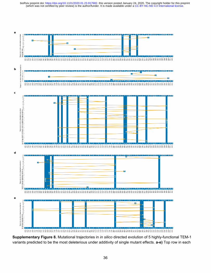
Supplementary Figure 8. Mutational trajectories in in silico directed evolution of 5 highly-functional TEM-1 variants predicted to be the most deleterious under additivity of single mutant effects. a-e) Top row in each

36

.CC-BY-NC-ND 4.0 International license(which was not certified by peer review) is the author/funder. It is made available under aThe copyright holder for this preprintthis version posted January 24, 2020. . https://doi.org/10.1101/2020.01.23.917682doi: bioRxiv preprint

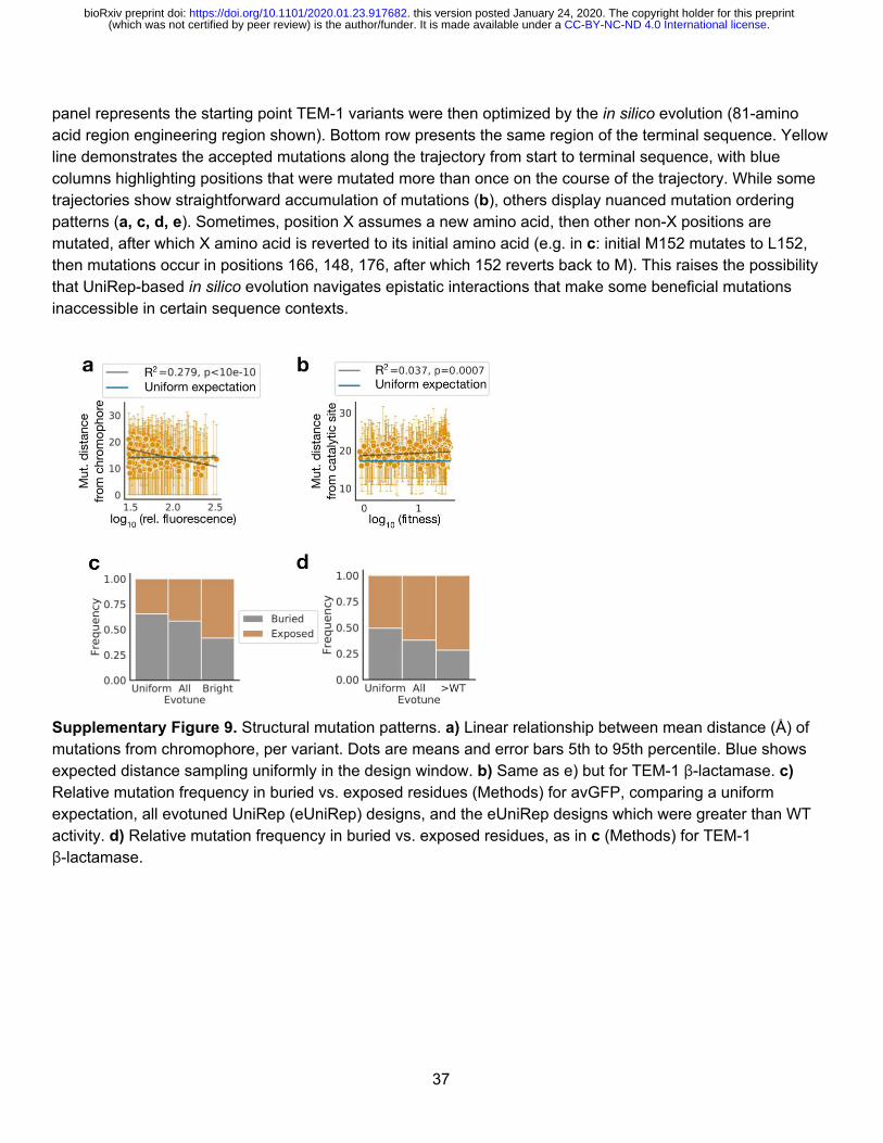
panel represents the starting point TEM-1 variants were then optimized by the in silico evolution (81-amino acid region engineering region shown). Bottom row presents the same region of the terminal sequence. Yellow line demonstrates the accepted mutations along the trajectory from start to terminal sequence, with blue columns highlighting positions that were mutated more than once on the course of the trajectory. While some trajectories show straightforward accumulation of mutations (b), others display nuanced mutation ordering patterns (a, c, d, e ). Sometimes, position X assumes a new amino acid, then other non-X positions are mutated, after which X amino acid is reverted to its initial amino acid (e.g. in c : initial M152 mutates to L152, then mutations occur in positions 166, 148, 176, after which 152 reverts back to M). This raises the possibility that UniRep-based in silico evolution navigates epistatic interactions that make some beneficial mutations inaccessible in certain sequence contexts.

Supplementary Figure 9. Structural mutation patterns. a) Linear relationship between mean distance (Å) of mutations from chromophore, per variant. Dots are means and error bars 5th to 95th percentile. Blue shows expected distance sampling uniformly in the design window. b) Same as e) but for TEM-1 β -lactamase. c) Relative mutation frequency in buried vs. exposed residues (Methods) for avGFP, comparing a uniform expectation, all evotuned UniRep (eUniRep) designs, and the eUniRep designs which were greater than WT activity. d) Relative mutation frequency in buried vs. exposed residues, as in c (Methods) for TEM-1 β -lactamase.

37

.CC-BY-NC-ND 4.0 International license(which was not certified by peer review) is the author/funder. It is made available under aThe copyright holder for this preprintthis version posted January 24, 2020. . https://doi.org/10.1101/2020.01.23.917682doi: bioRxiv preprint

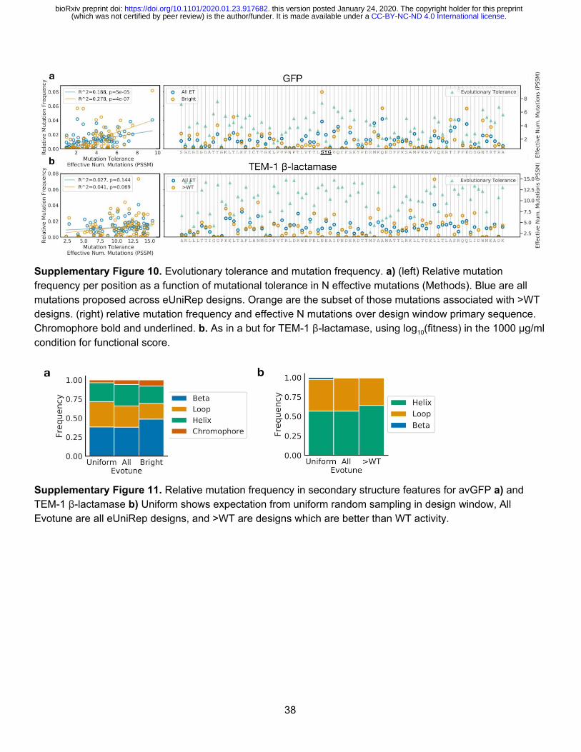
Supplementary Figure 10. Evolutionary tolerance and mutation frequency. a) (left) Relative mutation frequency per position as a function of mutational tolerance in N effective mutations (Methods). Blue are all mutations proposed across eUniRep designs. Orange are the subset of those mutations associated with >WT designs. (right) relative mutation frequency and effective N mutations over design window primary sequence. Chromophore bold and underlined. b. As in a but for TEM-1 β -lactamase, using log 10(fitness) in the 1000 μg/ml condition for functional score.

Supplementary Figure 11. Relative mutation frequency in secondary structure features for avGFP a) and TEM-1 β -lactamase b) Uniform shows expectation from uniform random sampling in design window, All Evotune are all eUniRep designs, and >WT are designs which are better than WT activity.

38

.CC-BY-NC-ND 4.0 International license(which was not certified by peer review) is the author/funder. It is made available under aThe copyright holder for this preprintthis version posted January 24, 2020. . https://doi.org/10.1101/2020.01.23.917682doi: bioRxiv preprint

Supplementary Figure 12. eUniRep-guided low-N design demonstrates the strongest generalization performance shown to date. In this analysis, we define generalization performance to be how often a method discovers >WT sequences within a search region of a given size, while controlling for the number of training data mutants. We tabulated these quantities from this work and 11 previous machine learning guided-protein design studies. a) Scatter plot illustrating the relationship between the size of the search region each study explored and the study’s hit rate normalized to the log 10 number of functionally characterized mutants used for training. Hit rate is normalized to the size of the training set in this manner because we a priori expect hit rate would improve with larger training sets. Most studies were organized along a “front” (gray line), suggesting an inherent trade-off between the size of the search space and the likelihood of finding high-functioning variants (controlling for training set size). eUniRep-guided low-N design (this work) managed this trade-off substantially better achieving normalized hit-rates that other approaches require a 10 15 to 10 25 smaller search region for. b) Qualitative descriptors of the machine learning methods used in each study. Most studies were interpolative, such that their training sequence distribution overlapped with the sequence distribution they aimed to generalize to. The remaining studies, including ours, were extrapolative and generalized to regions of the fitness landscape beyond the training distribution. Additionally, a few of the approaches require structural data, whereas the others, including ours, do not.

39

.CC-BY-NC-ND 4.0 International license(which was not certified by peer review) is the author/funder. It is made available under aThe copyright holder for this preprintthis version posted January 24, 2020. . https://doi.org/10.1101/2020.01.23.917682doi: bioRxiv preprint