low-cost visual/inertial hybrid motion capture system for
TRANSCRIPT

Low-Cost Visual/Inertial Hybrid Motion CaptureSystem for Wireless 3D Controllers
by
Alexander Wong
A thesis
presented to the University of Waterloo
in fulfilment of the
thesis requirement for the degree of
Master of Applied Science
in
Electrical and Computer Engineering
Waterloo, Ontario, Canada, 2007
c© Alexander Wong 2007

I hereby declare that I am the sole author of this thesis. This is a true copy of the
thesis, including any required final revisions, as accepted by my examiners.
I understand that my thesis may be made electronically available to the public.
ii

Abstract
It is my thesis that a cost-effective motion capture system for wireless 3D con-
trollers can be developed through the use of low-cost inertial measurement devices
and camera systems. Current optical motion capture systems require a number of
expensive high-speed cameras. The use of such systems is impractical for many ap-
plications due to its high cost. This is particularly true for consumer-level wireless
3D controllers. More importantly, optical systems are capable of directly track-
ing an object with only three degrees of freedom. The proposed system attempts
to solve these issues by combining a low-cost camera system with low-cost micro-
machined inertial measurement devices such as accelerometers and gyro sensors to
provide accurate motion tracking with a full six degrees of freedom. The proposed
system combines the data collected from the various sensors in the system to obtain
position information about the wireless 3D controller with 6 degrees of freedom.
The system utilizes a number of calibration, error correction, and sensor fusion
techniques to accomplish this task. The key advantage of the proposed system is
that it combines the high long-term accuracy and low frequency nature of the cam-
era system and complements it with the low long-term accuracy and high frequency
nature of the inertial measurement devices to produce a system with a high level
of long-term accuracy with detailed high frequency information about the motion
of the wireless 3D controller.
iii

Acknowledgements
First, let me start by thanking God for giving me strength in my research.
Secondly, I wish to thank my supervisors Professor William Bishop and Wayne
Loucks. In particular, I with to thank Professor William Bishop for his advice
and moral support throughout my time under his supervision. He has contributed
tremendously to my growth as a dedicated researcher.
I wish to thank all of the funding agencies and corporations that supported my
research through financial and knowledge support. In particular, I wish to thank
Epson Canada Ltd., and the Natural Sciences and Engineering Research Council
(NSERC) of Canada. I wish to especially thank Ian Clarke and Hui Zhou for
making the collaboration with Epson Canada Ltd. possible as well as invigorating
my love for research.
Finally, I wish to thank my family (especially my mother Rosemary and my
sister Scarlett), my friends and the colleagues at both University of Waterloo and
Epson Canada Ltd. for their unconditional support.
iv

Contents
1 Introduction 1
1.1 Motivation . . . . . . . . . . . . . . . . . . . . . . . . . . . . . . . . 2
1.2 Statement of Thesis . . . . . . . . . . . . . . . . . . . . . . . . . . . 4
1.3 Outline of the Thesis . . . . . . . . . . . . . . . . . . . . . . . . . . 6
2 Background 7
2.1 Magnetic Motion Capture Systems . . . . . . . . . . . . . . . . . . 7
2.2 Mechanical Motion Capture Systems . . . . . . . . . . . . . . . . . 8
2.3 Optical Motion Capture Systems . . . . . . . . . . . . . . . . . . . 10
2.4 Inertial Motion Capture Systems . . . . . . . . . . . . . . . . . . . 11
2.5 Hybrid Motion Capture Systems . . . . . . . . . . . . . . . . . . . . 13
3 Motion Capture System 14
3.1 Introduction . . . . . . . . . . . . . . . . . . . . . . . . . . . . . . . 14
3.2 Structural Overview . . . . . . . . . . . . . . . . . . . . . . . . . . 16
3.2.1 Hardware . . . . . . . . . . . . . . . . . . . . . . . . . . . . 16
3.2.2 Software . . . . . . . . . . . . . . . . . . . . . . . . . . . . . 19
4 Inertial Measurement Unit (IMU) 22
4.1 Introduction . . . . . . . . . . . . . . . . . . . . . . . . . . . . . . . 23
4.2 Background Theory . . . . . . . . . . . . . . . . . . . . . . . . . . . 25
v

4.3 IMU Structural Overview . . . . . . . . . . . . . . . . . . . . . . . 27
4.4 Sources of Error and Error Model . . . . . . . . . . . . . . . . . . . 29
4.5 Rate Gyro Error Evaluation . . . . . . . . . . . . . . . . . . . . . . 32
4.5.1 Experimental Results . . . . . . . . . . . . . . . . . . . . . . 34
4.6 Accelerometer Error Evaluation . . . . . . . . . . . . . . . . . . . . 36
4.6.1 Experimental Results . . . . . . . . . . . . . . . . . . . . . . 37
5 Inertial Navigation Unit (INU) 40
5.1 Introduction . . . . . . . . . . . . . . . . . . . . . . . . . . . . . . . 41
5.2 INU Structural Overview . . . . . . . . . . . . . . . . . . . . . . . . 42
5.3 Angular Velocity Processing Unit . . . . . . . . . . . . . . . . . . . 43
5.3.1 Frame of Reference Calibration . . . . . . . . . . . . . . . . 43
5.3.2 Data Integration and Error Reduction . . . . . . . . . . . . 45
5.4 Acceleration Processing Unit . . . . . . . . . . . . . . . . . . . . . . 46
5.4.1 Error Reduction . . . . . . . . . . . . . . . . . . . . . . . . . 47
5.4.2 Frame of Reference Transformation . . . . . . . . . . . . . . 47
5.4.3 Data Integration . . . . . . . . . . . . . . . . . . . . . . . . 52
6 Visual Tracking Unit (VTU) 54
6.1 Introduction . . . . . . . . . . . . . . . . . . . . . . . . . . . . . . . 54
6.2 VTU Structural Overview . . . . . . . . . . . . . . . . . . . . . . . 56
6.3 Object Detection . . . . . . . . . . . . . . . . . . . . . . . . . . . . 56
6.4 Position Estimation . . . . . . . . . . . . . . . . . . . . . . . . . . . 64
6.5 Experimental Results . . . . . . . . . . . . . . . . . . . . . . . . . . 67
7 Vision-Inertial Fusion Unit (VIFU) 69
7.1 Introduction . . . . . . . . . . . . . . . . . . . . . . . . . . . . . . . 69
7.2 Sensor Fusion Techniques . . . . . . . . . . . . . . . . . . . . . . . . 72
7.2.1 Complementary Filters . . . . . . . . . . . . . . . . . . . . . 72
vi

7.2.2 Kalman Filters . . . . . . . . . . . . . . . . . . . . . . . . . 73
7.3 VIFU Structural Overview . . . . . . . . . . . . . . . . . . . . . . . 76
7.4 Error-State Complementary Kalman Filter . . . . . . . . . . . . . . 76
8 Conclusions 82
8.1 Thesis Contributions . . . . . . . . . . . . . . . . . . . . . . . . . . 83
8.2 Potential for Future Research . . . . . . . . . . . . . . . . . . . . . 84
8.2.1 Low-Cost Multi-Marker Visual-Inertial Motion Capture . . . 84
8.2.2 Mainstream Software Applications Utilizing Motion Capture 85
8.3 Thesis Applicability . . . . . . . . . . . . . . . . . . . . . . . . . . . 85
Bibliography 86
vii

List of Tables
2.1 Comparison of existing motion capture techniques . . . . . . . . . . 13
4.1 Summary of orientation accuracy tests . . . . . . . . . . . . . . . . 34
4.2 Summary of position accuracy tests . . . . . . . . . . . . . . . . . . 37
6.1 Specifications of the test camera system . . . . . . . . . . . . . . . 68
6.2 Summary of VTU position accuracy test . . . . . . . . . . . . . . . 68
7.1 Summary of position accuracy tests . . . . . . . . . . . . . . . . . . 80
viii

List of Figures
3.1 Hardware setup of the proposed motion capture system . . . . . . . 18
3.2 Setup of the wireless 3D controller . . . . . . . . . . . . . . . . . . . 19
3.3 Overall software architecture of the proposed motion capture system 20
4.1 Operation of a piezoelectric-based vibrating gryo sensor . . . . . . . 24
4.2 3D tri-axis coordinate system . . . . . . . . . . . . . . . . . . . . . 25
4.3 3D orientation as represented using Euler angles . . . . . . . . . . . 26
4.4 Device frame of reference . . . . . . . . . . . . . . . . . . . . . . . . 28
4.5 Camera frame of reference . . . . . . . . . . . . . . . . . . . . . . . 28
4.6 Sample test trial from position accuracy tests . . . . . . . . . . . . 39
5.1 INU setup . . . . . . . . . . . . . . . . . . . . . . . . . . . . . . . . 42
5.2 Sample calibration alignment . . . . . . . . . . . . . . . . . . . . . 44
5.3 Effect of constant bias removal . . . . . . . . . . . . . . . . . . . . . 48
5.4 Frame of reference transform . . . . . . . . . . . . . . . . . . . . . . 50
6.1 VTU setup . . . . . . . . . . . . . . . . . . . . . . . . . . . . . . . 56
6.2 A cylindrical visualization of the HSV colour . . . . . . . . . . . . . 58
6.3 Initial colour thresholding of video frame . . . . . . . . . . . . . . . 60
6.4 Classic Hough transform of a line . . . . . . . . . . . . . . . . . . . 61
6.5 Circular Hough transform of a point . . . . . . . . . . . . . . . . . 63
6.6 Results of object detection . . . . . . . . . . . . . . . . . . . . . . . 65
ix
6.7 Inverted pinhole camera model . . . . . . . . . . . . . . . . . . . . . 66
7.1 Complementary filter system . . . . . . . . . . . . . . . . . . . . . . 73
7.2 VIFU setup . . . . . . . . . . . . . . . . . . . . . . . . . . . . . . . 77
7.3 Error-state complementary Kalman filter . . . . . . . . . . . . . . . 78
7.4 Position error over time for error-state complementary Kalman filter 81
x

Chapter 1
Introduction
This dissertation presents the design of a low-cost motion capture system using
both optical sensors and inertial sensors. Previous research has demonstrated the
effectiveness of such multi-sensor hybrid systems. The goal of this research is to
investigate and analyze the issues related to the design of such hybrid systems for
the purpose of tracking wireless input devices such as pen-based controllers. Such a
system provides a higher level of interactivity and control with respect to absolute
position and orientation of the 3D controller. This dissertation provides practical
solutions to the issues involved in the development of the proposed system such as
error reduction and correction, managing different frames of reference, and sensor
data fusion.
1

CHAPTER 1. INTRODUCTION
1.1 Motivation
Motion capture (or motion tracking) is the process of recording the movements of
an object. Motion capture systems are widely used in many diverse fields such as:
Animation – Motion capture systems have been used to capture the movements
of humans and animals to both enhance the realism of computer animated
characters in movies and video games. The other main benefit of motion
capture for use in movies and video games is that it can reduce the cost of
animation by eliminating the need for individual frames to be drawn by hand.
Medical – Motion capture systems have also been used in the medical field for a
number of different applications. One such application is the early diagno-
sis of movement-related disorders such as Parkinson’s disease [YAG+03] and
Multiple Sclerosis. Another application in the medical field is in biomechan-
ical research, where motion capture devices allow medical scientists to study
the mechanics of human motion to get a better understanding of how motion
behaviour relates to disease formation.
Simulation/Augmented Reality – Motion capture systems have also been used
to improve the realism of simulations and other augmented reality applica-
tions. By capturing the movement of the user, it is possible to dynamically
adapt the simulation to reflect the user’s actions. For example, wearable mo-
tion capture devices have been designed to track head movement. This allows
a simulation to change what is displayed on a display based on the direction
the user is looking.
Sports – Motion capture systems have primarily been used in sports for the pur-
2
CHAPTER 1. INTRODUCTION
pose of motion analysis. The motion of an athlete is recorded while he or she
is performing an action, such as hitting a ball or performing a jump. This
motion data is then analyzed to suggest changes to the way the athlete moves
to improve his or her efficiency and performance.
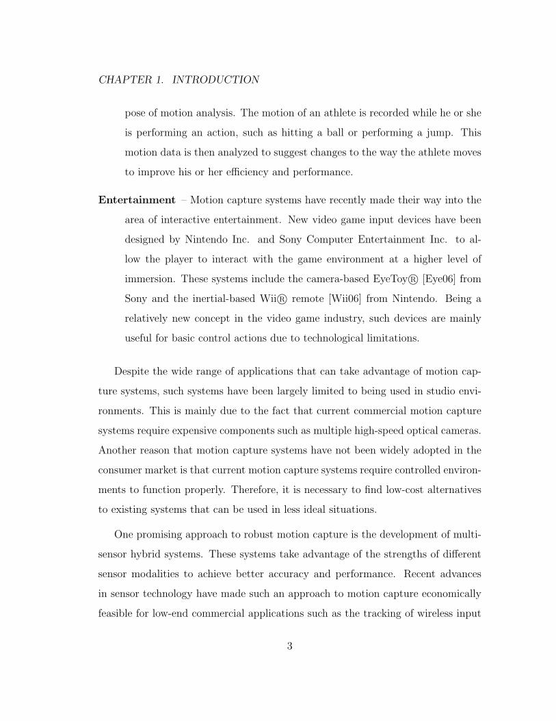
Entertainment – Motion capture systems have recently made their way into the
area of interactive entertainment. New video game input devices have been
designed by Nintendo Inc. and Sony Computer Entertainment Inc. to al-
low the player to interact with the game environment at a higher level of
immersion. These systems include the camera-based EyeToy R© [Eye06] from
Sony and the inertial-based Wii R© remote [Wii06] from Nintendo. Being a
relatively new concept in the video game industry, such devices are mainly
useful for basic control actions due to technological limitations.
Despite the wide range of applications that can take advantage of motion cap-
ture systems, such systems have been largely limited to being used in studio envi-
ronments. This is mainly due to the fact that current commercial motion capture
systems require expensive components such as multiple high-speed optical cameras.
Another reason that motion capture systems have not been widely adopted in the
consumer market is that current motion capture systems require controlled environ-
ments to function properly. Therefore, it is necessary to find low-cost alternatives
to existing systems that can be used in less ideal situations.
One promising approach to robust motion capture is the development of multi-
sensor hybrid systems. These systems take advantage of the strengths of different
sensor modalities to achieve better accuracy and performance. Recent advances
in sensor technology have made such an approach to motion capture economically
feasible for low-end commercial applications such as the tracking of wireless input
3

CHAPTER 1. INTRODUCTION
devices. Advances in Micro-Electro-Mechanical Systems (MEMS) have lead to the
development of miniature, low-cost inertial devices such as gyros and accelerom-
eters. Furthermore, advances have also been made in Charged Coupled Device
(CCD) manufacturing has lead to low-cost digital camera systems.
Low-cost inertial sensors such as gyros and accelerometers are capable of col-
lecting accurate data over short periods of time at a high sample rate. However,
error accumulates over time when the measurements captured by these devices are
used to obtain displacement and orientation information. Therefore, systems that
rely solely on low-cost inertial sensors are unable to maintain long-term accuracy.
On the other hand, low-cost camera sensors are capable of providing accurate mea-
surements over a long period of time. However, due to the amount of processing
involved in extracting and interpreting information from visual data obtained from
cameras, systems that rely solely on visual data can only operate at a low sample
rate. Therefore, inertial and visual sensing can be viewed as complementary sen-
sor technologies as each have different strengths that compensate for each other’s
weaknesses. As such, a system that combines both visual and inertial sensors has
the potential to provide more robust and accurate motion capture capabilities than
if they were used separately. Therefore, the main goal of the research presented by
this dissertation is to develop a hybrid motion capture system using both inertial
and visual sensors.
1.2 Statement of Thesis
It is my thesis that a hybrid vision-inertial approach to motion capture has the
potential to provide superior tracking information of wireless 3D controllers when
4

CHAPTER 1. INTRODUCTION
compared to a system consisting of only vision sensors or inertial sensors. A hybrid
system makes it possible for the use of low-cost off-the-shelf sensor components to
provide accurate, detailed, and robust 3D motion tracking. Furthermore, such a
system can operate reliably at a high resolution in non-ideal environments such
as an office or a home. This in turn opens up the possibility for consumer-level,
wireless 3D controllers that can provide absolute position and orientation in 3D
space and thus allows for a greater level of interactivity.
The design of a vision-inertial system for low-cost 3D motion tracking of wireless
3D controllers poses a number of different challenges. These include measurement
error reduction and prediction, coordinate system calibration, and data fusion.
As such, the proposed system is broken into separate components, each dealing
with a specific challenge. This modularization allows different sensors, filters, and
processing units to be removed and added according to the needs of the specific
device.
In some respects, the concept of the proposed system is similar to that proposed
in [SYA99], where vision and inertial data are fused to provide improved motion
tracking robustness and accuracy. However, the underlying goal is very different.
The system proposed in [SYA99] utilizes the motion tracking information for the
purpose of augmented reality registration and therefore focuses on tracking the
environment to align it with a virtual environment based on the point of view of
the user. Therefore, both the vision sensors and inertial sensors are centralized
at the user. However, the goal of this thesis research is to utilize motion tracking
information for the purpose of tracking a wireless 3D controller with respect to the
environment. As such, the vision sensors and inertial sensors are decentralized in
the proposed system to accommodate for object tracking.
5

CHAPTER 1. INTRODUCTION
1.3 Outline of the Thesis
Chapter 2 presents a background overview of existing motion capture systems.
Chapter 3 presents an overview of the hardware and software architecture of the
proposed motion capture system. Chapter 4 describes the inertial measurement unit
(IMU) in detail. The sources of error associated with rate gyros and accelerome-
ters used in the IMU are presented along with an error model for inertial sensors.
Furthermore, experimental results from stationary and dynamic error evaluation
tests are presented and analyzed in detail. Chapter 5 describes the design of the
inertial navigation unit (INU) used to determine relative 3D position and orien-
tation information from the raw data provided by the IMU. The error reduction
techniques used in the INU and the corresponding test results are also presented.
Chapter 6 describes the design of the visual tracking unit (VTU) used to determine
absolute 3D position from the visual data acquired by the camera system. The
marker detection and position estimation methods are described in detail. Chap-
ter 7 describes the design of the vision-inertial fusion unit (VIFU) used to combine
the information from the VTU and INU into 3D position information that is more
detailed than that provided by the VTU and more accurate and robust than that
provided by the INU. Chapter 8 discusses the thesis contributions and potential
topics for future research.
6

Chapter 2
Background
A great deal of research has been conducted in the area of motion capture and
tracking. While a large number of different sensor technologies have been used,
motion capture and tracking technologies can be grouped into categories:
1. Magnetic,
2. Mechanical,
3. Optical, and
4. Inertial.
2.1 Magnetic Motion Capture Systems
In magnetic motion capture systems [Asc06, YAG+03, JOH00], magnetic sensors
are placed on the object being tracked. These sensors measure the magnetic field
7

CHAPTER 2. BACKGROUND
being generated by a magnetic transmitter. Based on these measurements, position
and orientation information can be calculated with respect to the transmitter. One
such system is the MotionStar magnetic motion capture system from Ascension
Technology Corp. [Asc06], which has been used for tasks such as joint parameter
estimation [JOH00]. There are a number of advantages to magnetic motion capture
systems. First, such systems are not affected by occlusion as optical systems are.
Furthermore, magnetic motion capture systems can measure absolute positioning
of an object in 3D space. However, there are also a number of disadvantages to
utilizing magnetic motion capture systems. First, the strength of magnetic fields
decreases greatly as the distance from the transmitter increases. This effectively
limits the motion capture area of such systems. Second, the data acquired through
this technique is generally more noisy than that obtained using optical systems.
Most importantly, magnetic motion capture systems are highly sensitive to mag-
netic interference, which may occur due to external wiring and/or multiple tracked
objects in close range. This makes it poorly suited for consumer-level motion track-
ing, which must be capable of operating in non-ideal environments such as homes.
2.2 Mechanical Motion Capture Systems
In mechanical motion capture systems, a rigid exoskeleton that contains sensors
at each joint is attached to the object being tracked (typically a person). When
the object moves, the mechanical segments of the exoskeleton move along with the
object. The motion of the mechanical segments is then recorded by the sensors
at the joints to determine the relative motion of the object. An example of a
mechanical motion capture system is the Gypsy5 motion capture system from An-
8

CHAPTER 2. BACKGROUND
imazoo [Ani06], which consists of 37 potentiometers and 17 joints and is designed
to be worn by a human for the purpose of motion capture. There are a number of
advantages to mechanical motion capture systems. First, since the system captures
relative motion at the joints, it is not affected by occlusion as optical systems are.
Secondly, such systems can acquire data at a high sampling rate as the sensed data
does not require a lot of processing to extract motion information. Finally, mechan-
ical motion capture systems consist primarily of plastic or metal rods for segments
and potentiometers for sensors. Therefore, these systems can be constructed at
relatively low cost when compared to optical systems.
There are a number of disadvantages to mechanical motion capture systems.
First, such systems are unable to directly measure the absolute positioning of an
object. While absolute positioning may be inferred based on information about
the original reference position, this imposes additional limitations on the range
of actions performed by the object. For example, the performer using such as
system is not allowed to jump if absolute positioning is required since the change in
absolute positioning cannot be inferred from the relative motion measured by the
system. Secondly, the need for an exoskeleton makes mechanical motion capture
systems cumbersome when compared to other motion capture techniques. Finally,
such systems are suitable only for objects with moveable joints such as human
performers. Therefore, such techniques are not suitable for tracking the motion of
rigid objects such as wireless 3D controllers.
9

CHAPTER 2. BACKGROUND
2.3 Optical Motion Capture Systems
In optical motion capture systems, a number of markers are placed on the object
being tracked. Optical cameras are then used to track the individual markers on the
object. The captured visual information is then processed by the motion capture
system and used to triangulate the 3D position of each individual marker. Optical
systems can be grouped into two categories: i) Passive, and ii) Active. In passive
optical systems such as those produced by Vicon [Vic06], retro-reflective markers
are placed on the object being tracked and strobe lights are then used to illuminate
the markers so that they can be tracked by the camera. The main advantage
of passive systems over active systems is that the markers placed on the object
being tracked does not contain any electronic equipment, thus allowing for more
flexibility in certain situations. In active optical systems such as the OPTOTRAK
systems from NDI [NDI06], the markers contain embedded emitters. For example,
the PhaseSpace motion capture system [Pha06] can track up to 128 unique active
LED markers. The main advantage of active systems over passive systems is that
each marker can be uniquely identified. This allows for faster resolution of marker
overlaps as well as reduce the processing time required to track and distinguish
individual markers. As a result, active systems can perform at higher speeds than
passive systems at the expense of increased cost and reduced convenience.
There are a number of advantages to the use of optical systems over other meth-
ods. First, optical motion capture systems can measure absolute positioning of an
object in 3D space. Second, the data obtained using such systems are in general
cleaner than other techniques. Optical systems are flexible in terms of placement
on the object and therefore allows for greater freedom of motion. Furthermore,
it allows for multiple objects to be tracked simultaneously. Despite all of these
10

CHAPTER 2. BACKGROUND
benefits, there are some notable disadvantages to optical motion capture systems.
First, optical systems are susceptible to the effects of marker occlusion. The effects
of occlusion can be reduced through interpolation as well as the addition of cam-
eras to reduce the probability of occlusion, but result in increased computational
and/or economical costs. Another disadvantage of optical systems is that they are
incapable of measuring 3D orientation in a direct manner. Orientation must be cal-
culated indirectly based on the relative positioning between neighboring markers.
Not only does this add to the computational cost of the system, it also makes it
impossible to determine orientation on objects that contain a single marker. This
makes the use of purely optical data ill-suited for tracking wireless 3D controllers
which may be marked at a single location. Finally, optical motion capture systems
require a greater amount of computational processing than other techniques due
to the complexity of extracting information from visual data and then determining
absolute positioning and orientation based on that information. This is particularly
true for passive systems, where the software must also distinguish between different
markers. As such, most passive systems cannot be operated in a real-time scenario.
Therefore, it is difficult to implement an optical system based solely on low-cost
cameras with a high level of detail in a real-world environment.
2.4 Inertial Motion Capture Systems
The final main category of motion capture systems are those based on inertial sensor
devices. In inertial motion capture systems, inertial sensors such as gyros and
accelerometers are used to measure the relative motion of the object being tracked.
Gyros are used to determine orientation while accelerometers are used to determine
11

CHAPTER 2. BACKGROUND
acceleration. By placing the sensors normal to each other, inertial motion capture
systems can determine the relative 3D orientation and position at a particular point.
Inertial motion capture systems have been used extensively for vehicle navigation
and tracking [JLA95,DGEE03] and human motion tracking [Lui02,Roe06]. There
are a number of advantages to the use of inertial motion capture systems. First,
it provides direct measurement in 6 degrees of freedom (DOF), which cannot be
achieved using an optical system. This makes it well suited for tracking both
3D position and orientation of rigid objects with a single sensor location, such as
wireless 3D controllers. Second, it is capable of acquiring motion data at a high
sampling rate, as well as requiring less processing power than optical systems. This
allows it to provide very detailed motion information. Furthermore, it is not affected
by visible occlusion. Finally, like optical systems the placement of sensors is flexible
and allows for the object to perform a greater range of motions. There are two main
disadvantages to inertial motion capture systems. First, like mechanical systems
they are unable to directly measure the absolute positioning of an object. This
imposes some limitations on the range of actions performed by the object. More
importantly, inertial sensors does not measure position and orientation explicitly,
but derives the information based on measured acceleration and angular velocity.
This leads to rapid error accumulation over time and therefore are stable only in
short periods of time. This makes error reduction and correction very crucial in
the design of an accurate inertial motion capture system.
12
CHAPTER 2. BACKGROUND
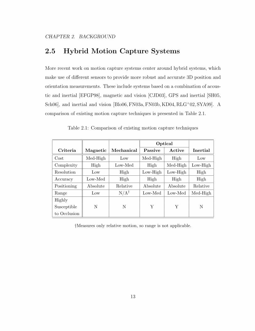
2.5 Hybrid Motion Capture Systems
More recent work on motion capture systems center around hybrid systems, which
make use of different sensors to provide more robust and accurate 3D position and
orientation measurements. These include systems based on a combination of acous-
tic and inertial [EFGP98], magnetic and vision [CJD03], GPS and inertial [SH05,
Sch06], and inertial and vision [Blo06, FN03a, FN03b,KD04, RLG+02, SYA99]. A
comparison of existing motion capture techniques is presented in Table 2.1.
Table 2.1: Comparison of existing motion capture techniques
OpticalCriteria Magnetic Mechanical Passive Active Inertial
Cost Med-High Low Med-High High Low
Complexity High Low-Med High Med-High Low-High
Resolution Low High Low-High Low-High High
Accuracy Low-Med High High High High
Positioning Absolute Relative Absolute Absolute Relative
Range Low N/A† Low-Med Low-Med Med-High
HighlySusceptible N N Y Y Nto Occlusion
†Measures only relative motion, so range is not applicable.
13

Chapter 3
Motion Capture System
This chapter briefly describes the overall architecture of the proposed motion cap-
ture system. The first section presents an introduction to the problems and issues
faced during the design of the system. Furthermore, the design philosophy behind
the proposed system architecture is presented. The next section provides a struc-
tural overview of the system, both on a hardware and software level. First, the
environment setup of the system is described in detail. Second, the placement of
sensors in the actual wireless 3D controller is presented. Finally, the architectural
overview of the underlying software processing system is described.
3.1 Introduction
The main goal of the motion capture system is to record and determine the 3D po-
sition and orientation of a wireless 3D controller using low-cost inertial and vision
sensors. In designing such a system, it is very important to identify the main chal-
14

CHAPTER 3. MOTION CAPTURE SYSTEM
lenges and issues involved in accomplishing the primary goal. The main challenges
in the design of the proposed system can be defined as follows:
Sensor Error – There are a number of different types of errors associated with
inertial sensors such as rate gyros and accelerometers. As described in Chap-
ter 2, inertial sensors do not measure position and orientation directly. Rate
gyros measure angular velocity and accelerometers measure linear accelera-
tion. To obtain actual position and orientation, it is necessary to perform
numerical integration on the raw data acquired by the accelerometers and
rate gyros respectively. Therefore, measurement error accumulates over time,
resulting in a rapid degradation of tracking accuracy. Methods to reduce error
accumulation is required for the system to perform with a reasonable level of
accuracy.
Change in Coordinate Frames – Inertial sensors are capable of measuring only
relative motion. As such, the measurements made by the inertial sensors
are with respect to the 3D controller upon which the sensors are mounted.
Therefore, a change in the orientation of the 3D controller causes a change
in the orientation of the inertial sensors. This is problematic as the data
measured by the inertial sensors will be with respect to the new coordinate
frame. Therefore, methods to transform the measured data from the different
coordinate frames to a common coordinate frame is required to determine the
absolute position of the 3D controller.
Sensor Fusion – The motion of the same 3D controller is measured by different
types of inertial sensors as well as the camera system. Therefore, a method to
combine the data gathered from different sensor sources is needed to produce
15

CHAPTER 3. MOTION CAPTURE SYSTEM
information that is more reliable and more detailed than that produced by
the individual sensor devices.
Visual Tracking – It is necessary to extract position information from the visual
data acquired by the camera system. Therefore, the system must detect the
3D controller from the acquired visual data as well as determine its absolute
position in an accurate and robust manner.
By defining the primary challenges, the proposed system can then be designed
to address each of these challenges in an effective and efficient manner.
3.2 Structural Overview
The proposed system utilizes both hardware and software components to determine
the final 3D position and orientation of the wireless 3D controller. The hardware
used is responsible for acquiring sensory data about the wireless 3D controller, while
the software is responsible for transforming the sensory data into usable 3D motion
information.
3.2.1 Hardware
An overview of the hardware setup of the proposed system is shown in Figure 3.1.
The proposed motion capture system consists of three main hardware components.
The first component is the camera system, which acquires visual data about the
3D controller with respect to the surrounding environment. For the purpose of the
proposed system, a single digital video camera was used to provide 2-D video feed-
back to the PC processing system. This is reasonable for consumer-level, human-
16

CHAPTER 3. MOTION CAPTURE SYSTEM
computer interfacing applications such as video game controllers and pen-based
input devices since the motion of the input devices often follow along a 2-D plane
at a close to medium range. For full 3D motion feedback, two or more digital
video cameras must be placed in precise locations to perform accurate triangula-
tion. However, such a complicated setup makes it difficult to integrate a multiple
camera system into a typical consumer-level environment, such as an office or a
home. Therefore, a single camera system is better suited for consumer-level 3D
controller tracking applications. The camera is positioned such that its optical axis
is parallel to the ground.
The second component of the motion capture system is the wireless 3D con-
troller, which is held by the human user and used to interface with a given applica-
tion. Applications that are well-suited for this type of system include applications
that utilize pen-based input devices and video games that support wireless 3D con-
trollers. These applications benefit from the greater degree of interaction that the
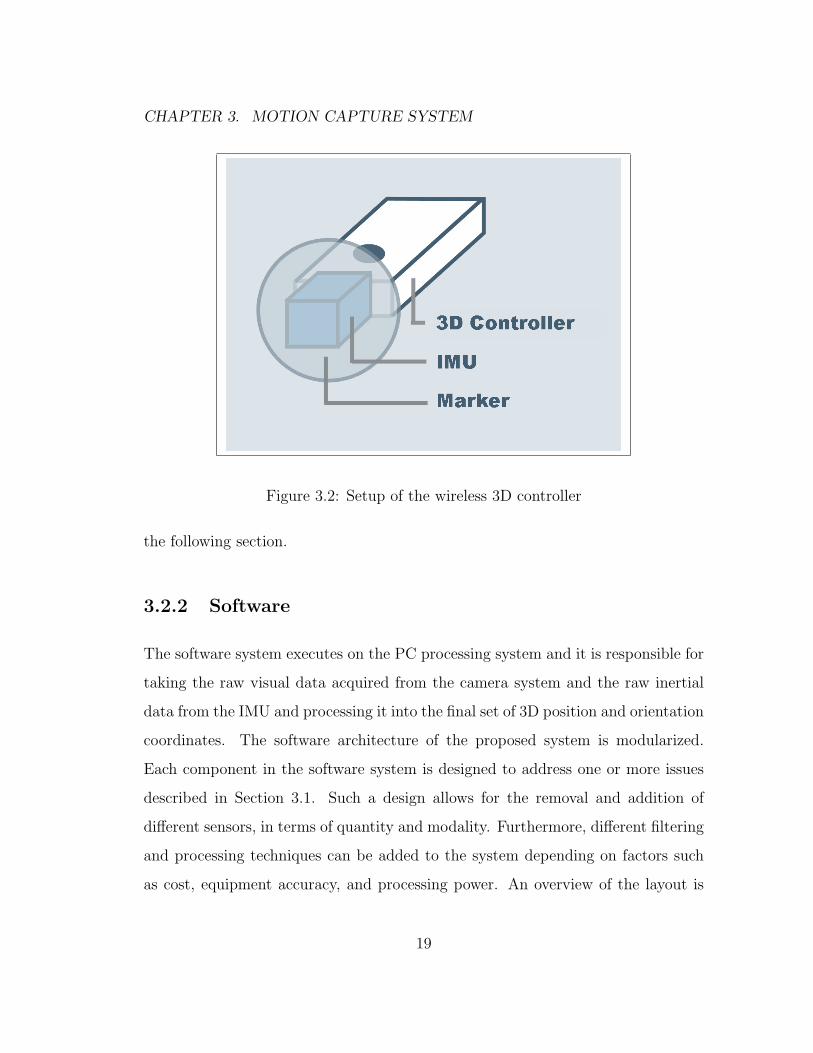
proposed system provides. A general layout of the wireless 3D controller is illus-
trated in Figure 3.2. A passive spherical marker is mounted to the front of the
wireless 3D controller. This marker allows the camera system to track the position
of the 3D controller. A series of miniature inertial sensors are embedded into the
wireless 3D controller to acquire 3D motion data with 6 degrees of freedom. The
set of inertial sensors is referred to as the inertial measurement unit (IMU). This
unit is described in further detail in Chapter 4.
The third and final component of the motion capture system is the PC process-
ing system, which receives visual data from the camera system and inertial data
from the IMU and processes it into a final set of 3D position and orientation co-
ordinates. The details of the software in the PC processing system is presented in
17

CHAPTER 3. MOTION CAPTURE SYSTEM
Figure 3.1: Hardware setup of the proposed motion capture system
18
CHAPTER 3. MOTION CAPTURE SYSTEM
Figure 3.2: Setup of the wireless 3D controller
the following section.
3.2.2 Software
The software system executes on the PC processing system and it is responsible for
taking the raw visual data acquired from the camera system and the raw inertial
data from the IMU and processing it into the final set of 3D position and orientation
coordinates. The software architecture of the proposed system is modularized.
Each component in the software system is designed to address one or more issues
described in Section 3.1. Such a design allows for the removal and addition of
different sensors, in terms of quantity and modality. Furthermore, different filtering
and processing techniques can be added to the system depending on factors such
as cost, equipment accuracy, and processing power. An overview of the layout is
19

CHAPTER 3. MOTION CAPTURE SYSTEM
shown in Figure 3.3.
Figure 3.3: Overall software architecture of the proposed motion capture system
The software system in the proposed motion capture system consists of three
main software components. The first component is the inertial navigation unit
(INU), which is responsible for taking raw 3D inertial data from the IMU and
transforming it into more consistent 3D position and orientation coordinates. To
achieve this goal, the INU must be capable of performing three main tasks. First,
it must take the raw inertial data and transform it into a consistent frame of
reference. Second, it must attempt to filter noise from the raw inertial data to
reduce error accumulation. Finally, it must take the linear acceleration and angular
velocity information acquired by the IMU and convert it to position and orientation
coordinates. The techniques used in the INU to perform these tasks are described
in further detail in Chapter 5.
20
CHAPTER 3. MOTION CAPTURE SYSTEM
The second component of the software system is the visual tracking unit (VTU),
which is responsible for taking the raw visual data from the camera system and ex-
tracting the 3D position of the wireless 3D controller. The VTU must be capable of
detecting and distinguishing the marker on the 3D controller from the surrounding
environment. Furthermore, based on the location of the detected marker in the
visual data the VTU must also be able to estimate the absolute location of the
marker in the real world. The techniques used in the VTU to perform these tasks
are described in further detail in Chapter 6.
The third and final component of the software system is the vision-inertial fusion
unit (VIFU). This unit is responsible for taking the processed 3D motion data
from the IMU and the VTU and combining them into a final set of 3D position
and orientation coordinates that is more detailed and stable than that obtained
from either of the individual sources. This processing involves using the individual
strengths of vision and inertial sensors to overcome the individual weaknesses of
each technique. The techniques used in the VIFU to accomplish this are described
in further detail in Chapter 7.
21

Chapter 4
Inertial Measurement Unit (IMU)
This chapter describes in detail the overall design and performance analysis of the
inertial measurement unit (IMU). Introductions to inertial sensors, coordinate sys-
tems and frames of reference are presented. These topics are essential to a complete
understanding of inertial sensor systems. A structural overview of the IMU is then
presented. The sources of error associated with inertial sensors are presented, along
with an error model which can then be used in the design of error reduction and
correction techniques. The results are presented for the error evaluation performed
on the gyro sensors and accelerometers in both static and dynamic situations. The
analysis and performance evaluation aids in the determination of the limitations of
the individual sensors in real-world situations.
22

CHAPTER 4. INERTIAL MEASUREMENT UNIT (IMU)
4.1 Introduction
An inertial sensor is a device that measures motion based on the general principles
of Newton’s Laws of Motion. Newton’s First Law of Motion states that an object
in a state of uniform motion tends to remain in that state of motion unless acted
upon by an unbalanced external force. By measuring the unbalanced force exerted
on the object, the motion of the system can be deduced in a number of different
ways. The two types of sensors that are most widely used in inertial motion sensing
are accelerometers and gyro sensors.
Accelerometers are inertial sensor devices designed to measure linear accelera-
tion. This is accomplished by measuring the force exerted on the sensor device and
calculating the corresponding acceleration based on the measured force. Based on
the calculated acceleration, the relative motion of the object can be determined.
Linear velocity can be obtained by integrating the acceleration of the object. By
performing a second integration, the position of the object can be determined. A
number of different types of accelerometers are available. Of particular interest
in recent years are accelerometers based on MEMS technology. Such devices are
small, robust, and can be manufactured at a low cost. MEMS accelerometers such
as those produced by Kionix [Kio06] are based on the principle of differential ca-
pacitance. A sensing element within the accelerometer moves in relationship with
a fixed element. When the sensing element moves, its distance from the fixed el-
ement changes and this results in a change in electrical capacitance. This change
in capacitance is then measured by the device and converted into a signal that is
proportional to the acceleration of the device.
Gyro sensors are inertial sensor devices that measure angular velocity. Similar
to accelerometers, gyro sensors measure the externally applied force and converts
23

CHAPTER 4. INERTIAL MEASUREMENT UNIT (IMU)
the force into the corresponding angular velocity. This can then be used to deter-
mine the orientation of the sensor by integrating the measured angular velocity.
A number of different types of gyro sensors have been developed, such as spin-
ning gyro sensors, laser gyro sensors, and vibrating gyro sensors. Of particular
interest are vibrating gyro sensors based on MEMS [ADBW02] and piezoelectric
technology [Boy05]. Vibrating gyro sensors can be made small, stable, and reli-
able. Vibrating gyro sensors utilize the Coriolis effect. In steady state, the sensing
element of the gyro sensor is forced to vibrate in a particular direction at a high
frequency. When angular rotation occurs, a Coriolis force is exerted and causes
the sensing element of the gyro sensor to move in a perpendicular direction to the
vibration direction. This produces a current that is proportional to the angular ve-
locity of the object. The operation of a piezoelectric-based gyro sensor is illustrated
in Figure 4.1.
Figure 4.1: Operation of a piezoelectric-based vibrating gryo sensor (Courtesy ofEpson)
It is important to note that, while both gyro sensors and accelerometers can
be used to measure position and orientation respectively, neither measure position
24

CHAPTER 4. INERTIAL MEASUREMENT UNIT (IMU)
and orientation in a direct manner. Therefore, it is necessary to further process the
inertial data obtained from the inertial sensors to obtain position and orientation
information.
4.2 Background Theory
Before describing the underlying setup of the IMU, it is important to provide a
brief introduction to the fundamentals of coordinate systems to fully understand
the measured data. In a common 3D coordinate system at an arbitrary frame of
reference, the position of an object in 3D space is defined by a tri-axis system
which consists of the x -axis, y-axis, and z -axis. A typical 3D coordinate system is
illustrated in Figure 4.2.
y
x
z
object(x,y,z)
(0,0,0)
Figure 4.2: 3D tri-axis coordinate system
25

CHAPTER 4. INERTIAL MEASUREMENT UNIT (IMU)
The orientation of an object in 3D space can be similarly defined using an
orientation system based on the above tri-axis system. This orientation system
consists of three parameters: i) roll, ii) pitch, and iii) yaw. Roll refers to a change
in orientation about the x -axis. Pitch refers to an orientation change about the y-
axis. Yaw refers to an orientation change about the z -axis. Positive values indicate
counter clockwise rotations about the corresponding axis. The aforementioned
orientation system is commonly represented using Euler angles by defining overall
orientation as an ordered combination of rotations using three angles (α, β, γ). A
rotation about the x -axis is denoted by α. A rotation about the y-axis is denoted
by β. Finally, a rotation about the z -axis is denoted by γ. This orientation system
representation is shown in Figure 4.3. Hence, a complete description of an object’s
motion can be summarized using six parameters (x,y,z for position, and α, β, γ for
orientation).
Figure 4.3: 3D orientation as represented using Euler angles
26

CHAPTER 4. INERTIAL MEASUREMENT UNIT (IMU)
It is also necessary to provide an explanation on the different frames of reference
used in the proposed motion capture system. This is because data acquired from
the different sensor components of the proposed system are collected in different
frames of reference. This makes it necessary to understand the different frames
of reference used so that the acquired data can be brought into a single frame of
reference for the purpose of data fusion. Two coordinate frames of reference are
used in the proposed motion capture system: i) the device frame, and ii) the camera
frame.
In the device frame of reference, the origin of the coordinate system is located
at the center of gravity of the IMU. The x -axis is pointed out of the front of the
wireless 3D controller. The y-axis points out of the left of the 3D controller and
the z -axis points out of the top of the controller. The device frame of reference is
illustrated in Figure 4.4.
In the camera frame of reference, the origin of the coordinate system is located at
the projection center of the camera system. The x -axis is points towards the camera
from the image plane. The y-axis points right from the camera’s perspective and
and the z -axis points upwards from the camera’s perspective. The camera frame of
reference is illustrated in Figure 4.5. The coordinate transformation from the device
frame of reference to the camera frame of reference is discussed in Section 5.3.1 and
Section 5.4.2 for the gyro sensors and accelerometers, respectively.
4.3 IMU Structural Overview
The IMU consists of six inertial sensors: three gyro sensors and three accelerom-
eters. The three gyro sensors are mounted in a tri-axis configuration to measure
27

CHAPTER 4. INERTIAL MEASUREMENT UNIT (IMU)
y
x
z
α
β
γ
Figure 4.4: Device frame of reference
y
x
z
y
x
z
y
x
z
y
x
z
Figure 4.5: Camera frame of reference
28
CHAPTER 4. INERTIAL MEASUREMENT UNIT (IMU)
angular velocity at three degrees of freedom in the device frame: i) roll, ii) pitch,
and iii) yaw. The three accelerometers are also mounted in a tri-axis configuration
to measure linear acceleration at three degrees of freedom in the device frame: i)
x -axis, ii) y-axis, and iii) z -axis. By combining the three gyro sensors and the three
accelerometers, the IMU can measure motion with six degrees of freedom. The IMU
is embedded in the center of the marker at the front of the wireless 3D controller.
For the test implementation of the motion capture system, a MicroStrain G-Link
2.4 GHz Wireless Accelerometer [Mic07] was provided courtesy of Epson Corpora-
tion to measure linear acceleration in 3D space. The accelerometers used within
the device are based on MEMS technology and have an acceleration range of ±2G
and a maximum sampling rate of 2,048 sweeps per second. Epson Corporation also
provided an InterSense Wireless InertiaCube3 [Int07] for the purpose of measuring
angular motion in 3D space. Based on the specifications provided by InterSense, the
device contains three gyro sensors and is capable of obtaining angular orientation
with a RMS accuracy of 0.25◦ for pitch at a temperature of 25 ◦C without system
enhancements enabled. All internal optimization settings for the device are turned
off to provide the best possible representation of the raw data from the built-in
sensors.
4.4 Sources of Error and Error Model
One of the main caveats to using inertial sensors for motion capture purpose is the
instability of such systems in long-term situations as a result of error accumulation.
Inertial sensors such as accelerometers and gyro sensors do not measure position
or orientation directly. To obtain the position and orientation of an object in
29

CHAPTER 4. INERTIAL MEASUREMENT UNIT (IMU)
3D space, integration must be performed on the measured data from the inertial
sensors. This is particularly problematic for accelerometers since the acquired data
must be integrated twice to obtain position information. Errors in acceleration
measurement increase the position error quadratically. Therefore, it is necessary to
reduce and correct the associated error to obtain accurate position information.
To develop proper error filtering and correction methods, it is necessary to
identify and understand the underlying sources of error associated with the inertial
sensors used in the IMU. This allows for the formulation of error models for rep-
resenting these sources of error. Sources of error associated with inertial sensors
such as accelerometers and gyro sensors can be generalized into four categories: i)
scaling factor error, ii) gravity-related error, iii) manufacturing-related error, and
iv) time-varying error. Both gyro sensors and accelerometers are susceptible to
scaling factor errors, manufacturing-related errors, and time-varying errors, while
gravity-related errors apply to accelerometers only.
It is typically the case that the raw data acquired from an inertial sensor is
proportional to but not equal to the actual motion. It is necessary to scale the
measured data by a scaling factor to obtain the actual motion. A suggested scaling
factor is usually not provided by the manufacturer. Therefore, a scaling factor must
be determined experimentally for a specific sensor. An incorrect scaling factor or
a change in scaling factor results in an error that is proportional to the difference
between the actual and incorrect scaling factors. The sensor model of an inertial
sensor with a scaling factor error can be represented as:
xmeasured = (1 + escale)xactual (4.1)
where xmeasured is the measured sensor output, escale is the scaling factor error, and
30

CHAPTER 4. INERTIAL MEASUREMENT UNIT (IMU)
xactual is the actual sensor output. Fortunately, it was found in [GE04] that external
factors have minimal effects on the scaling factor of inertial sensors. For a simplified
error model, it is not required to account for scaling factor errors.
The second source of error is related to changes in local gravitational effects.
As previously discussed, accelerometers measure external forces directly but do
not measure acceleration directly. The force of acceleration can be determined as
follows:
aactual = ameasured − g (4.2)
where aactual is the actual acceleration force, ameasured is the measured acceleration
force, and g is the gravitational force acting on the sensor. It is necessary to remove
the effects of gravity to obtain the actual acceleration of the object. Gravitational
force is often represented by the gravitational constant. However, gravitational force
actually varies depending on the location of the object. As a result, the use of a fixed
gravitational term results in inaccurate acceleration measurements. Fortunately,
this form of error can be corrected during the calibration of the proposed motion
capture system by measuring the actual gravitational force at the specific location
and using it to remove gravitational effects. Therefore, gravitational effects can be
taken into account during the calibration process.
The third source of error is related to particularities in the manufacturing pro-
cess of the individual sensors. Defects and imperfections in the inertial sensor
devices can lead to measurement biases that result in error accumulation. A re-
lated source of error is the degradation of device performance due to wear. Over
time, inertial sensors within a device may become misaligned or damaged from ex-
cessive use. This type of error must be taken into account in the error model and
can be modeled effectively as a constant offset econstant.
31

CHAPTER 4. INERTIAL MEASUREMENT UNIT (IMU)
The final source of error is related to error sources that vary over time. These
include electrical noise, sampling noise, and device sensitivity errors. To simplify the
overall error model, time-varying error sources are grouped into two categories: i)
sampling noise (esampling(t)), and ii) non-sampling noise (evary(t)). This is sufficient
for the proposed motion capture system because a vision-based system with good
long-term stability is used to improve and complement the results acquired from
the IMU.
Based on the above descriptions, a general error model that is suitable for both
the gyro sensors and accelerometers used in the proposed motion capture system
can be expressed as:
xmeasured = xactual + e (4.3)
e = econstant + evary(t) + esampling(t) (4.4)
where xmeasured is the measured value, xactual is the actual value, e is the overall error,
econstant is the constant bias, evary(t) is the time-varying error bias, and esampling(t)
is the sampling error.
4.5 Rate Gyro Error Evaluation
A total of four tests were performed to validate the accuracy of the gyro sensor
when compared with the specifications provided by the manufacturer. The tests
were designed to test a variety of different scenarios, with two controlled tests that
can be easily replicated and two uncontrolled tests based on random motion. The
uncontrolled tests are more representative of real-world scenarios and therefore
reflect the actual real-world performance of the device to a greater degree. Ten
32

CHAPTER 4. INERTIAL MEASUREMENT UNIT (IMU)
trials were performed for each of the tests to improve the statistical accuracy of the
results. Below is a description of each of the four tests:
Test 1: In this controlled test, the pitch orientation of the device is changed by
a total of 10◦ in 3 s, while the yaw and roll orientations are left unchanged. This
test is performed to test the device under motion in a single plane and to validate
whether the device is capable of producing accurate results under small orientation
changes.
Test 2: In this controlled test, the pitch orientation of the device is changed by
a total of 360◦, while the yaw and roll orientations are left unchanged. This results
in a net orientation change of 0◦ in pitch. This test is performed to test the device
to validate whether the device is capable of producing accurate results under large
changes in orientation.
Test 3: In this uncontrolled test, the pitch, yaw, and roll orientations of the
device are changed continuously in a random fashion at a random rate for a period
of 10 s. By controlling the final pitch orientation of the testing apparatus, the net
orientation change is 30◦ in terms of pitch orientation. This test is performed to
test the device to validate whether the device is capable of maintaining accurate
orientation states under sporadic rotational changes over a very short period of
time. This test validates the short-term reliability of the gyro sensor device.
Test 4: In this uncontrolled test, the pitch, yaw, and roll orientations of the
device are changed continuously in a random fashion at a random rate for a period
of 2 minutes. By controlling the final pitch orientation of the testing apparatus, the
net orientation change is 30◦ in terms of pitch orientation. This test is performed
to test the device to validate whether the device is capable of maintaining accurate
orientation states under sporadic rotational changes over a longer period of time
33

CHAPTER 4. INERTIAL MEASUREMENT UNIT (IMU)
when compared to the previous test. Furthermore, the 10 trials for this test are
performed consecutively without resetting the device to evaluate the accumulated
error over a long period of time. The total testing time was measured to be 26
minutes from the start of the first trial to the end of the last trial. This test
validates the long-term reliability of the sensor device.
4.5.1 Experimental Results
A summary of the orientation accuracy results of Tests 1 to 4 is shown in Table 4.1.
It can be observed that the gyro sensor device performs well within the specifications
in three of the four test scenarios. In the first test, the RMS error is very small
and within range of the provided specifications. In the second and third tests, the
RMS error is higher than the first test. However, it is still very small and within
the range of the provided specifications. From the perspective of a consumer-
level application, the differences in RMS error amongst the first three tests can
be considered negligible. Therefore, it is evident that the sensor device is capable
of producing accurate results in short-term scenarios in the presence of different
orientation changes and different sporadic motions.
Test Actual Net Mean RMS Error Error AccumulatedNo. Orientation Measured Standard Error
Orientation Deviation(Degrees) (Degrees) (Degrees) (Degrees) (Degrees)
1 10 9.910 0.3034 0.1704 -2 0 0.341 0.4341 0.2831 -3 30 30.139 0.3587 0.2229 -4 30 29.805 0.8393 0.4329 6.410
Table 4.1: Summary of orientation accuracy tests
34

CHAPTER 4. INERTIAL MEASUREMENT UNIT (IMU)
Based on the accuracy results of Test 4, it can be observed that the resulting
RMS error is noticeably higher than that provided by InterSense. It can also
be observed that the accumulated error is noticeable over the test period of 26
minutes. Furthermore, the accumulated error result validates that the error of
the gyro sensors increases linearly with respect to time. While the accumulated
error of the device can be considered small for a consumer-level application such
as the proposed motion capture system, this does indicate that the accumulated
error begins to have a noticeable influence on orientation accuracy when the usage
period is extended to a longer period of time (i.e., hours). As such, it is necessary
to provide the user with a means to recalibrate the wireless 3D controller after
an extended period of usage to maintain accuracy. The error accumulation of the
gyro sensor device is linear and given the accuracy of the device and the accuracy
needed for the application it can be used for over an hour without the need for
recalibration in its current state. Simple noise filtering techniques can be used to
further extend this time period without recalibration.
It is evident from the experimental results that low-cost gyro sensor devices
such as the InterSense Wireless InertiaCube3 are capable of producing accurate
orientation measurements. The device is relatively stable over a reasonably long
period of time without aid or recalibration. This makes it well-suited for use in the
proposed motion capture system, since the vision system is not capable of providing
useful information regarding the orientation of the 3D controller.
35

CHAPTER 4. INERTIAL MEASUREMENT UNIT (IMU)
4.6 Accelerometer Error Evaluation
A total of four tests were performed to validate the accuracy of the accelerometer
device under a number of different scenarios. The four tests are designed to evaluate
the static positioning accuracy of the device over an extended period of time. The
relative position of the device based on the measured acceleration was calculated by
finding the double integral of the measured data. The constant bias was estimated
from long-term data and subtracted from the acceleration data. A number of trials
were performed for each test to improve statistical accuracy of the results. Each
test was conducted for a maximum of 65,500 sweeps due to the memory storage
limitations of the device. A description of the tests are provided as follows:
Test 1: In this static position accuracy test, the device is left in a fixed location
with no external forces being exerted on the device. The device is configured to
measure a total of 65,500 sweeps at 2,048 sweeps/second, resulting in a total mea-
surement time period of 31.98 s. This test is performed to evaluate the accumulated
error of the device and its effect on position measurement over a shorter period of
time at a high sampling rate. A total of 10 trials were conducted.
Test 2: In this static position accuracy test, the device is left in a fixed location
with no external forces being exerted on the device. The device is configured to
measure for 65,500 sweeps at 1,024 sweeps/second, resulting in a total measurement
time period of 63.96 s. A total of 10 trials were conducted.
Test 3: In this static position accuracy test, the device is left in a fixed location
with no external forces being exerted on the device. The device is configured to
measure for 65,500 sweeps at 512 sweeps/second, resulting in a total measurement
time period of 127.93 s. A total of 10 trials were conducted.
36
CHAPTER 4. INERTIAL MEASUREMENT UNIT (IMU)
Test 4: In this static position accuracy test, the device is left in a fixed location
with no external forces being exerted on the device. The device is configured to
measure for 65,500 sweeps at 256 sweeps/second, resulting in a total measurement
time period of 255.86 s. This test is performed to evaluate the accumulated error
of the device and its effect on position measurement over a longer period of time
at a low sampling rate. A total of 10 trials were conducted.
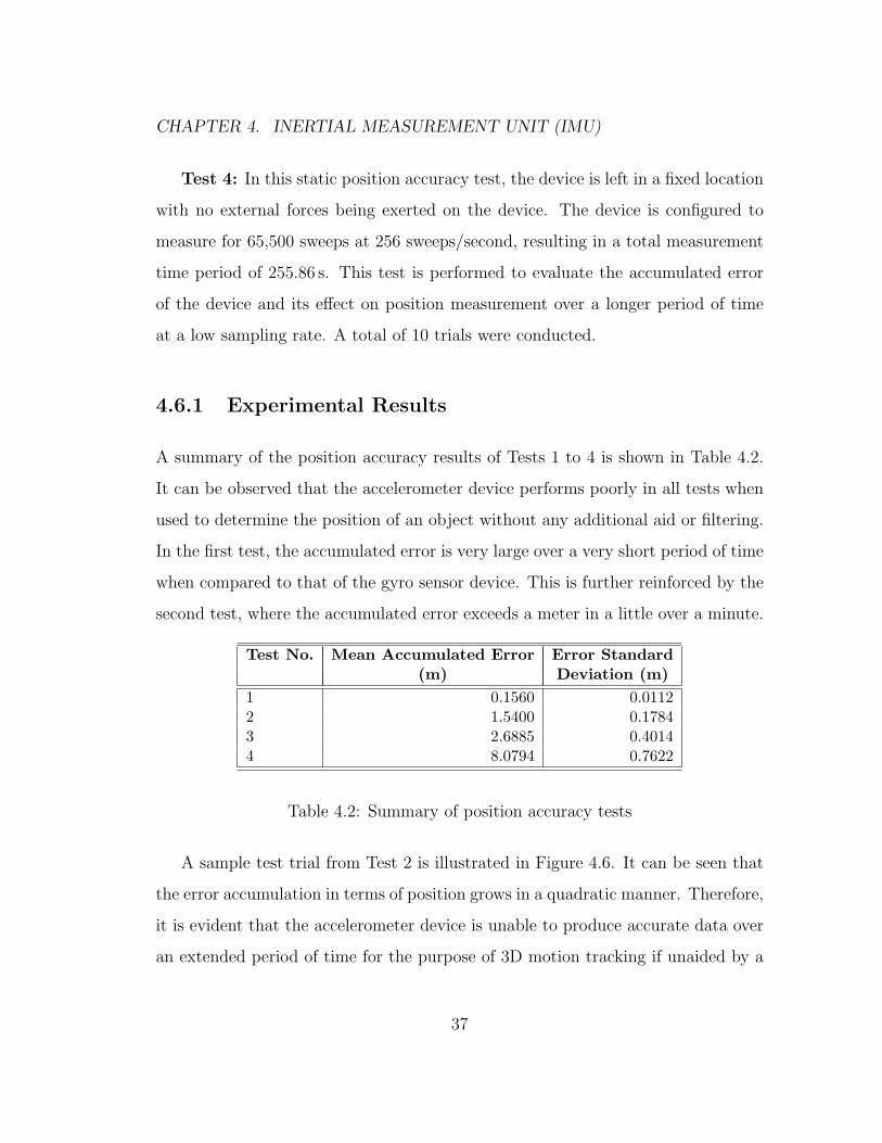
4.6.1 Experimental Results
A summary of the position accuracy results of Tests 1 to 4 is shown in Table 4.2.
It can be observed that the accelerometer device performs poorly in all tests when
used to determine the position of an object without any additional aid or filtering.
In the first test, the accumulated error is very large over a very short period of time
when compared to that of the gyro sensor device. This is further reinforced by the
second test, where the accumulated error exceeds a meter in a little over a minute.
Test No. Mean Accumulated Error Error Standard(m) Deviation (m)
1 0.1560 0.01122 1.5400 0.17843 2.6885 0.40144 8.0794 0.7622
Table 4.2: Summary of position accuracy tests
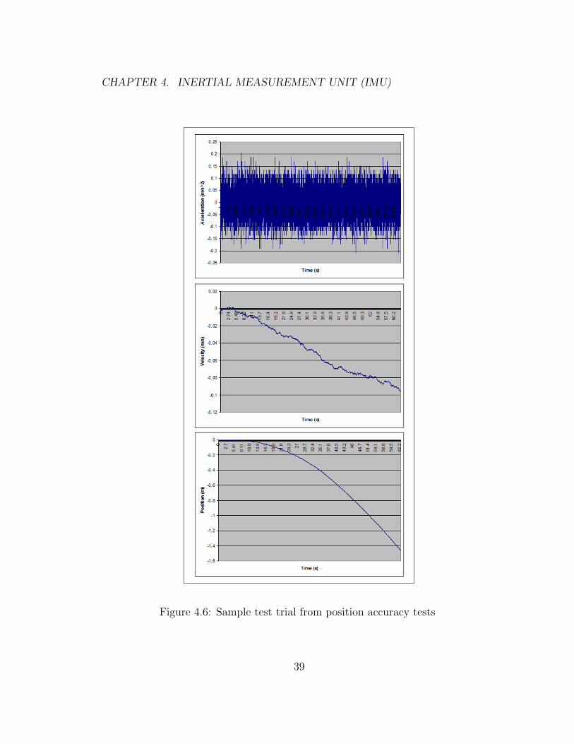
A sample test trial from Test 2 is illustrated in Figure 4.6. It can be seen that
the error accumulation in terms of position grows in a quadratic manner. Therefore,
it is evident that the accelerometer device is unable to produce accurate data over
an extended period of time for the purpose of 3D motion tracking if unaided by a
37

CHAPTER 4. INERTIAL MEASUREMENT UNIT (IMU)
secondary device. Fortunately, the vision system in the proposed motion capture
system can be used to provide error correction for the inertial system.
It is evident that the accelerometer device is capable of acquiring many samples
over a short period of time, resulting in a detailed description of the motion of an
object. However, it is also clear that it is highly unstable in the long-term when
used for determining position information. This indicates that error filtering and
correction is necessary if one desires highly detailed and accurate results. These
techniques are discussed in Chapter 5 and Chapter 7.
38
CHAPTER 4. INERTIAL MEASUREMENT UNIT (IMU)
Figure 4.6: Sample test trial from position accuracy tests
39

Chapter 5
Inertial Navigation Unit (INU)
This chapter describes in detail the overall design of the inertial navigation unit
(INU). The first section presents an introduction to inertial navigation systems.
The next section provides a structural overview of the INU. The data transfor-
mation systems used for gyro and accelerometer data are described in Section 5.3
and Section 5.4, respectively. Section 5.3.1 provides a discussion on calibrating the
angular velocity data from the device frame of reference with the camera frame of
reference. Section 5.3.2 describes integration and error reduction techniques used
to convert angular velocity information into orientation information. Section 5.4.1
describes the error reduction performed for the accelerometer data in the INU. Sec-
tion 5.4.2 describes the theory used to transform linear acceleration data from the
device frame of reference to the camera frame of reference. Section 5.4.3 presents the
integration techniques used to convert linear acceleration information into position
information.
40

CHAPTER 5. INERTIAL NAVIGATION UNIT (INU)
5.1 Introduction
An inertial navigation system (INS) is a system that computes motion information
using measurements made by inertial sensor devices such as accelerometers and gyro
sensors. To accomplish this goal, the INS must be capable of performing a number
of important tasks. Navigation systems such as GPS and optical systems [KGK02]
calculate position and orientation information in a direct manner for the purpose of
deriving other motion characteristics such as velocity and acceleration. Unlike these
systems, an INS must deduce position and orientation information in an indirect
manner from the linear acceleration and angular velocity information provided by
the inertial sensor devices. This is accomplished in an INS by performing a double
integration on the linear acceleration data to obtain position and a single integration
on the angular velocity data to obtain orientation.
Inertial sensors are capable of measuring only relative motion. Data obtained
from these inertial devices can be said to be in a device frame of reference. For
the proposed system, it is necessary to obtain absolute position and orientation
information from a camera frame of reference. Therefore, the INS is responsible
for transforming the inertial data from the device frame of reference to the camera
frame of reference. Finally, due to the errors associated with inertial sensor devices
(particularly accelerometers), the INS must also provide error reduction capabilities
for the resulting position and orientation information to be useful.
41
CHAPTER 5. INERTIAL NAVIGATION UNIT (INU)
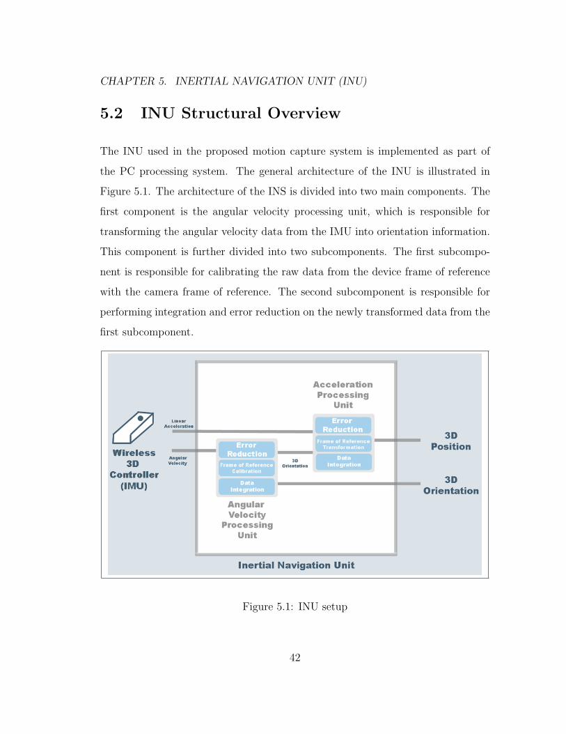
5.2 INU Structural Overview
The INU used in the proposed motion capture system is implemented as part of
the PC processing system. The general architecture of the INU is illustrated in
Figure 5.1. The architecture of the INS is divided into two main components. The
first component is the angular velocity processing unit, which is responsible for
transforming the angular velocity data from the IMU into orientation information.
This component is further divided into two subcomponents. The first subcompo-
nent is responsible for calibrating the raw data from the device frame of reference
with the camera frame of reference. The second subcomponent is responsible for
performing integration and error reduction on the newly transformed data from the
first subcomponent.
Figure 5.1: INU setup
42

CHAPTER 5. INERTIAL NAVIGATION UNIT (INU)
The second component is the acceleration processing unit, which is responsible
for transforming linear accelerometer data from the IMU into position information.
The linear accelerometer processing unit is divided into two subcomponents. The
first subcomponent utilizes the orientation information from the angular velocity
processing unit to transform the linear acceleration data from the device frame
of reference to the camera frame of reference. The second subcomponent then
takes the transformed acceleration data and integrates the data to obtain position
information. Furthermore, the second subcomponent is responsible for performing
error reduction on the acceleration data.
5.3 Angular Velocity Processing Unit
The angular velocity processing unit takes angular velocity information from the
gyro sensor device and transforms it into 3D orientation information.
5.3.1 Frame of Reference Calibration
To transform the angular velocity information from the device frame of reference to
the camera frame of reference, it is necessary to know the initial orientation of the
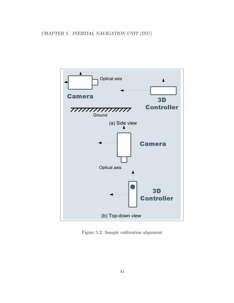
wireless 3D controller. This is accomplished through a device calibration process
where the user is informed to hold the wireless 3D controller in a horizontal manner
such that the bottom face of the device is parallel to the ground and the front of
the device points towards the camera. This effectively aligns the device with the
camera whose optical axis is set such that it runs parallel to the ground. A sample
calibration alignment is illustrated in Figure 5.2. This orientation is then recorded
as the origin orientation in the camera frame of reference.
43
CHAPTER 5. INERTIAL NAVIGATION UNIT (INU)
(a) Side view
(b) Top-down view
Optical axis
Optical axis
Ground
Figure 5.2: Sample calibration alignment
44
CHAPTER 5. INERTIAL NAVIGATION UNIT (INU)
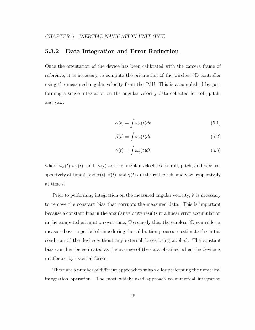
5.3.2 Data Integration and Error Reduction
Once the orientation of the device has been calibrated with the camera frame of
reference, it is necessary to compute the orientation of the wireless 3D controller
using the measured angular velocity from the IMU. This is accomplished by per-
forming a single integration on the angular velocity data collected for roll, pitch,
and yaw:
α(t) =∫
ωα(t)dt (5.1)
β(t) =∫
ωβ(t)dt (5.2)
γ(t) =∫
ωγ(t)dt (5.3)
where ωα(t), ωβ(t), and ωγ(t) are the angular velocities for roll, pitch, and yaw, re-
spectively at time t, and α(t), β(t), and γ(t) are the roll, pitch, and yaw, respectively
at time t.
Prior to performing integration on the measured angular velocity, it is necessary
to remove the constant bias that corrupts the measured data. This is important
because a constant bias in the angular velocity results in a linear error accumulation
in the computed orientation over time. To remedy this, the wireless 3D controller is
measured over a period of time during the calibration process to estimate the initial
condition of the device without any external forces being applied. The constant
bias can then be estimated as the average of the data obtained when the device is
unaffected by external forces.
There are a number of different approaches suitable for performing the numerical
integration operation. The most widely used approach to numerical integration
45

CHAPTER 5. INERTIAL NAVIGATION UNIT (INU)
involves the use of Newton-Cotes formulas (e.g., Trapezoid rule, Simpson’s rule,
etc.). A more advanced approach to numerical integration involves the use of
Gaussian quadratures (e.g., Gauss-Hermite, Gauss-Legendre, etc.), which provide
greater flexibility (i.e., support for non-uniformly spaced samples) and accuracy at
the cost of higher computational overhead than the Newton-Cotes formulas. Since
data is acquired at equally spaced intervals by the IMU, the Newton-Cotes approach
provides good accuracy at a low computational cost. For the proposed system, the
Simpson’s Rule was used to perform numerical integration on the inertial data as it
provides a good balance between efficiency and accuracy, especially given that fact
that the acquired data is read sequentially without further subsampling. Simpson’s
Rule approximates the area under a curve using a series of quadratic polynomials.
The resulting formula for computing orientation from angular velocity for a specific
axis (roll, pitch, yaw) is given by the following:
n∫0
θ(t)dt ≈n−1
2∑k=1
h
3[ω(2k − 1) + 4ω(2k) + ω(2k + 1)] + O(h5f (4)(k)) (5.4)
where h = ∆t is the sampling period, θ is the orientation angle for a particular
axis, and ω is the angular velocity for the chosen axis. The O(h5f (4)(k)) term is a
remainder term that is approximately 0 for small values of h.
5.4 Acceleration Processing Unit
The acceleration processing unit takes linear acceleration information from the
accelerometer device and transforms it into 3D position information.
46

CHAPTER 5. INERTIAL NAVIGATION UNIT (INU)
5.4.1 Error Reduction
Prior to performing a frame of reference transformation on the measured linear
acceleration data, it is necessary to remove the constant bias that corrupts the
measured data. This is important because a constant bias in the acceleration data
results in an exponential error accumulation in the computed position over time.
To remedy this, the wireless 3D controller is measured over a period of time during
the calibration process to determine the initial condition of the device without any
external forces being applied. To accomplish this, the effects of gravity are first
subtracted from the measurements of the IMU. The constant bias can then be esti-
mated as an average of the data obtained when the device is unaffected by external
forces and subtracted from the acceleration data. The effect of constant bias re-
moval is illustrated in Figure 5.3. It is clear from the figure that the accumulated
error is significantly reduced after the constant bias removal process. Note that the
vertical axis scale of the first figure is much greater than the vertical axis scale of
the 2nd figure due to the accumulated error introduced by the constant bias.
5.4.2 Frame of Reference Transformation
The raw acceleration data from the IMU is acquired in the device frame of reference.
As such, the data from IMU is able to describe relative motion and not absolute
motion in the environment as needed by the motion capture system. Therefore, it
is necessary to transform the linear acceleration information from the device frame
of reference to the camera frame of reference. The first step is to determine the
initial position of the device in the camera frame of reference to serve as the 3D
position offset of the device. This is accomplished at the calibration stage, when
47

CHAPTER 5. INERTIAL NAVIGATION UNIT (INU)
Figure 5.3: Effect of constant bias removal
48

CHAPTER 5. INERTIAL NAVIGATION UNIT (INU)
the camera system determines the initial position of the device in the camera frame
of reference. The initial position coordinates are denoted by (x0,y0,z0).
The second step in transforming 3D acceleration data from the device frame
of reference to the camera frame of reference is to determine the transformation
model that relates the two frames of reference. This is accomplished through the
use of 3D orientation data that was computed by the angular velocity processing
unit. The transformation model from the camera frame of reference to the device
frame of reference and vice versa at a particular point in time can be defined as an
series of rotations performed in a consecutive fashion. In the case of Euler angles,
the transformation model from the camera frame of reference to the device frame
of reference can be represented as a sequence of yaw (γ), pitch (β), and roll (α).
This is illustrated in Figure 5.4.
The net frame of reference transform from the camera frame of reference to the
device frame of reference can be formulated as a direction cosine matrix (DCM)
Rdevicecamera as follows:
Rdevicecamera = R(α)R(β)R(γ) (5.5)
where
R(α) =
1 0 0
0 cos(α) − sin(α)
0 sin(α) cos(α)
(5.6)
49

CHAPTER 5. INERTIAL NAVIGATION UNIT (INU)
y
z
x
Yaw (γ)
z'
y'
x'
y'
x'
z'
Pitch (β)
x''
z''
y''
x''
z''
Roll (α)
y''
x'''
z'''
y'''
Figure 5.4: Frame of reference transform
50
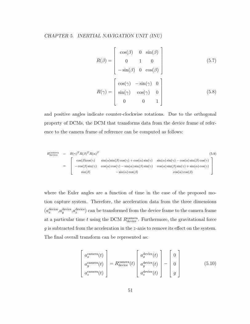
CHAPTER 5. INERTIAL NAVIGATION UNIT (INU)
R(β) =
cos(β) 0 sin(β)
0 1 0
− sin(β) 0 cos(β)
(5.7)
R(γ) =
cos(γ) − sin(γ) 0
sin(γ) cos(γ) 0
0 0 1
(5.8)
and positive angles indicate counter-clockwise rotations. Due to the orthogonal
property of DCMs, the DCM that transforms data from the device frame of refer-
ence to the camera frame of reference can be computed as follows:
Rcameradevice = R(γ)T R(β)T R(α)T (5.9)
=
cos(β)cos(γ) sin(α)sin(β) cos(γ) + cos(α) sin(γ) sin(α) sin(γ) − cos(α) sin(β) cos(γ)
− cos(β) sin(γ) cos(α) cos(γ) − sin(α) sin(β) sin(γ) cos(α) sin(β) sin(γ) + sin(α) cos(γ)
sin(β) − sin(α) cos(β) cos(α) cos(β)
where the Euler angles are a function of time in the case of the proposed mo-
tion capture system. Therefore, the acceleration data from the three dimensions
(adevicex ,adevice
y ,adevicez ) can be transformed from the device frame to the camera frame
at a particular time t using the DCM Rcameradevice . Furthermore, the gravitational force
g is subtracted from the acceleration in the z-axis to remove its effect on the system.
The final overall transform can be represented as:
acamera
x (t)
acameray (t)
acameraz (t)
= Rcameradevice (t)
adevice
x (t)
adevicey (t)
adevicez (t)
−
0
0
g
(5.10)
51

CHAPTER 5. INERTIAL NAVIGATION UNIT (INU)
5.4.3 Data Integration
Once the acceleration data has been transformed from the device frame of reference
to the camera frame of reference, it is necessary to compute the position of the
wireless 3D controller using the measured linear acceleration data from the IMU.
This is accomplished by performing a double integration on the linear acceleration
data collected for the x, y, and z-axes:
x(t) =∫ ∫
ax(t)dt2 (5.11)
y(t) =∫ ∫
ay(t)dt2 (5.12)
z(t) =∫ ∫
az(t)dt2 (5.13)
where ax(t), sy(t), and az(t) are the linear acceleration in the camera frame of
reference for the x, y, and z-axis respectively at time t, and x(t), y(t), and z(t) are
the position coordinates at time t. As with the angular velocity processing unit, the
Simpson’s Rule approach to numerical integration is used to compute the position
information. The resulting formula for computing position from acceleration for a
specific axis (x, y, and z) is given by the following:
n∫0
v(t)dt ≈n−1
2∑k=1
h
3[a(2k − 1) + 4a(2k) + a(2k + 1)] + O(h5f (4)(k)) (5.14)
n∫0
p(t)dt ≈n−1
2∑k=1
h
3[v(2k − 1) + 4v(2k) + v(2k + 1)] + O(h5f (4)(k)) (5.15)
52

CHAPTER 5. INERTIAL NAVIGATION UNIT (INU)
where h = ∆t is the sampling period, p is the position for a particular axis, and v
and a are the linear velocity and linear acceleration respectively for that axis. The
O(h5f (4)(k)) term is a remainder term that is approximately 0 for small values of
h.
The final step to computing the 3D position in the camera frame of reference is
to add the initial position offset recorded during the calibration process described
in Section 5.4.2:
x′
y′
z′
=
x
y
z
+
x0
y0
z0
(5.16)
53

Chapter 6
Visual Tracking Unit (VTU)
This chapter describes in detail the overall design of the visual tracking unit (VTU).
The first section presents an introduction to vision tracking systems. Section 6.2
provides a structural overview of the VTU. The object detection techniques used in
the VTU are described in Section 6.3. Section 6.4 presents the techniques used to
determine the position of the wireless 3D controller in the camera frame of reference.
Finally, Section 6.5 present experimental results using the proposed VTU system.
6.1 Introduction
Visual tracking is the process of tracking one or more objects through the use of a
optical device such as a camera system. Visual tracking has been used in a wide
range of applications. These include: face tracking [SZM03], head tracking [ML-
CVA00, MJVR03], patient motion tracking [BGS+05], and augmented reality for
medical procedures [VKS06]. Visual tracking systems can be divided into two gen-
54

CHAPTER 6. VISUAL TRACKING UNIT (VTU)
eral groups. The first group are those that do not use markers for visual tracking.
Such techniques rely on image registration and other complex computer vision tech-
niques to track the motion of the desired object(s) and/or environment. Marker-less
techniques are typically more computationally expensive. The second group of vi-
sual tracking systems are those that make use of distinctive markers placed on the
object or environment being tracked. These techniques are typically less complex
as markers are significantly easier to detect and track with greater accuracy. The
visual tracking unit implemented in the proposed motion capture system is based
on a marker tracking scheme where a marker placed at the front of the wireless 3D
controller is tracked visually by a camera system.
The purpose and the overall design of the proposed motion capture system helps
simplify the task of visually tracking the wireless 3D controller. First, the wireless
3D controller contains a single marker of uniform colour that needs to be tracked. As
such, the object detection process can be simplified and the amount of processing
required is effectively reduced. Second, the marker mounted on the wireless 3D
controller for the purpose of tracking is a solid sphere. As such, its shape is invariant
to rotation and thus reduce the complexity of the tracking system. Furthermore,
the visual tracking system is used in conjunction with an inertial tracking system
to eliminate the need for complex motion and orientation interpolation techniques.
Finally, the purpose of the motion capture system is to allow for improved human-
computer interactivity at close range to mid range distances. Therefore, the marker
is close enough to the camera system that the size of the marker can be determined
by the system. This size information is particularly useful for improving the position
estimate.
55
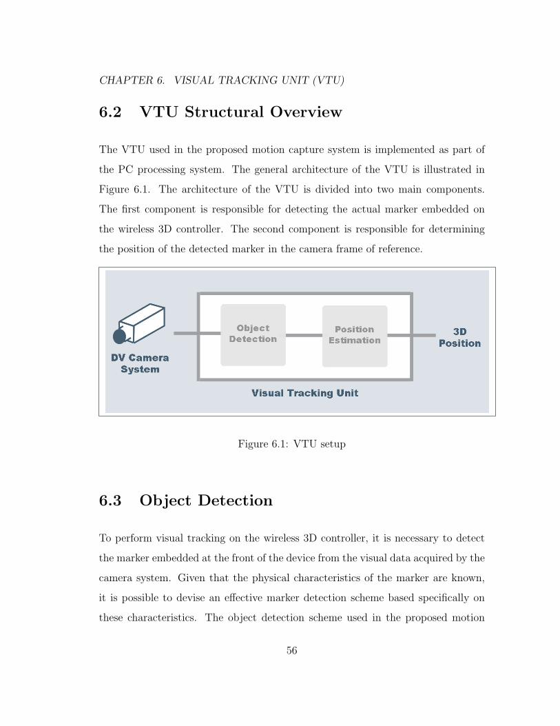
CHAPTER 6. VISUAL TRACKING UNIT (VTU)
6.2 VTU Structural Overview
The VTU used in the proposed motion capture system is implemented as part of
the PC processing system. The general architecture of the VTU is illustrated in
Figure 6.1. The architecture of the VTU is divided into two main components.
The first component is responsible for detecting the actual marker embedded on
the wireless 3D controller. The second component is responsible for determining
the position of the detected marker in the camera frame of reference.
Figure 6.1: VTU setup
6.3 Object Detection
To perform visual tracking on the wireless 3D controller, it is necessary to detect
the marker embedded at the front of the device from the visual data acquired by the
camera system. Given that the physical characteristics of the marker are known,
it is possible to devise an effective marker detection scheme based specifically on
these characteristics. The object detection scheme used in the proposed motion
56

CHAPTER 6. VISUAL TRACKING UNIT (VTU)
capture system is based on two important characteristics of the marker: i) colour,
and ii) shape.
The first characteristic of the marker that is analysed by the object detection
system is colour. Since the colour of the marker is uniform and known a priori,
it is possible to reduce the search space and data in a particular video frame by
first performing colour thresholding on the frame. There are a number of issues
that must be considered before colour thresholding can be performed. The low-cost
camera system used in the proposed motion capture system captures video content
in the Red-Green-Blue (RGB) colour space. This colour space represents colour
as a combination of additive primary colours. One issue associated with the RGB
colour space with regards to its representation of colour is that the channels in the
colour space are not easily separable.
The first issue related to this is that the RGB colour space is less intuitive for
describing specific pure colours. This makes it more difficult to calibrate the system
to detect the specific uniform colour ranges associated with the marker. The second
and more important issue that needs to be dealt with is the problem of varying
lighting conditions. Since the channels of the RGB colour space do not explicitly
characterize illumination as an individual characteristic, the RGB value for an
object under high illumination can be significantly different than if it was under
low illumination as the colour and brightness of a pixel are coupled. One effective
approach to addressing both these issues is to transform the colour information from
the RGB colour space to the Hue-Saturation-Value (HSV) colour space. The HSV
colour space represents colour as a combination of three components: i) Hue, ii)
Saturation, and iii) Value. Hue represents a pure colour within the visible spectrum.
Saturation represents the colour intensity of hue. The greater the saturation, the
57
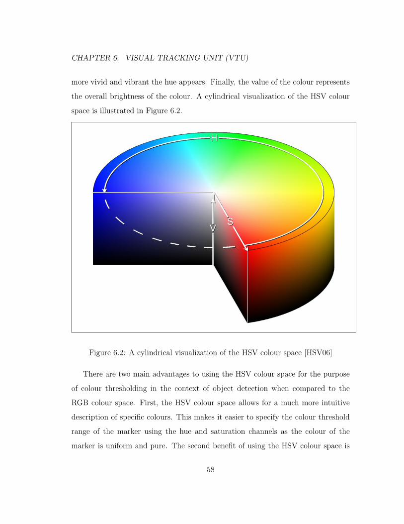
CHAPTER 6. VISUAL TRACKING UNIT (VTU)
more vivid and vibrant the hue appears. Finally, the value of the colour represents
the overall brightness of the colour. A cylindrical visualization of the HSV colour
space is illustrated in Figure 6.2.
Figure 6.2: A cylindrical visualization of the HSV colour space [HSV06]
There are two main advantages to using the HSV colour space for the purpose
of colour thresholding in the context of object detection when compared to the
RGB colour space. First, the HSV colour space allows for a much more intuitive
description of specific colours. This makes it easier to specify the colour threshold
range of the marker using the hue and saturation channels as the colour of the
marker is uniform and pure. The second benefit of using the HSV colour space is
58

CHAPTER 6. VISUAL TRACKING UNIT (VTU)
that the hue and saturation of colour are decoupled from the brightness of colour.
This allows for the colour threshold range of the marker to be specified independent
of the brightness levels making colour detection robust to changes in illumination.
In the proposed system, each video frame is converted from a RGB image into a
HSV image as well as a greyscale image. If a particular pixel in the HSV image
does not fall into the hue and saturation ranges specified for the target marker,
the equivalent pixel in the greyscale image is set to 0. This effectively isolates
the candidate pixels for the target marker in the greyscale image. The resulting
threshold greyscale image is processed using an edge detector to produce a binary
edge map of the scene. For the proposed system, the threshold image is first
smoothed using a Gaussian kernel to reduce noise and then processed using a Sobel
edge detector. The colour threshold and edge detection process is illustrated in
Figure 6.3.
Once the binary edge map of the scene is computed, the second characteristic of
the marker that is analysed is shape. Since the marker is in the shape of a sphere, it
appears in the 2D image plane as a circle regardless of the view angle. Therefore, the
marker can be detected as a circle in the binary edge map. One particularly robust
and effective technique for circle detection is the Circular Hough Transform [DH72].
The Hough transform is a common method used to provide a global description
of curve features in an image such as lines and circles. In the classical Hough
transform, the points in a binary image as defined in the xy coordinate space are
mapped into a coordinate space that is defined by the parameters of the curve
feature being represented. For the case of line features, points in the xy coordinate
space are mapped into a ρθ parameter space, where ρ and θ correspond to the
parameters of a line as defined by the line equation:
59

CHAPTER 6. VISUAL TRACKING UNIT (VTU)
a) Original frame
b) Initial threshold frame
Figure 6.3: Initial colour thresholding of video frame
60

CHAPTER 6. VISUAL TRACKING UNIT (VTU)
xcos(θ) + ysin(θ) = ρ (6.1)
where ρ represents the length of the normal vector going from the origin of the image
(typically defined as the top-left corner of the image) to the line and θ represents
the angular orientation of the normal vector with respect to the x-axis. In actual
implementation, the ρθ parameter space is discretized into what is referred as an
accumulator array. Each point in the xy coordinate space corresponds to a curve
in ρθ parameter space, while each point in the ρθ parameter space corresponds to
a line in the xy coordinate space. An example illustrating an xy to ρθ coordinate
space mapping using the Hough transform is illustrated in Figure 6.4. Therefore,
the value at location (ρ, θ) in the accumulator array represents the number of points
in the binary image that lies on the line defined by the parameters rho and theta.
Hence, line features can be recognized by detecting peaks in the accumulator array.
Figure 6.4: Classic Hough transform of a line
61

CHAPTER 6. VISUAL TRACKING UNIT (VTU)
A similar approach to the classic Hough transform is taken for the Circular
Hough Transform. Instead of the line equation, the parameters of a circle can be
defined by the following circle equation:
(x− xc)2 + (y − yc)
2 = r2 (6.2)
where xc and yc are the x and y coordinates of the center of the circle and r is
the radius of the circle. This results in a 3D parameter space as defined by the
parameters xc, yc, and r. For a fixed value of r, each point in the xy coordinate
space of the image contributes to the center points (xc, yc) of a set of possible circles
upon which the point lies on. This is illustrated in Figure 6.5. It can be clearly
seen that a point in the xy coordinate space maps to a circle with the radius of
r in the xc − yc − r parameter space for that specific radius. By computing the
parameter space for a range of radii, the parameters of the circle representing the
marker is determined as the global maximum of the 3D parameter space. The main
advantage of the Circular Hough Transform is that it is very robust against noise
and discontinuities, making it well suited for non-ideal scenarios such as real-world
environments.
While the search space was reduced using colour thresholding, the computation
of Circular Hough Transform can still be computationally expensive as it needs to
be computed for each radius. Therefore, a number of techniques were used to reduce
the computational cost of performing the Circular Hough Transform process.
The first technique used was simply to reduce the range of radii that can be
detected by the system. Since the purpose of the system is known, the range
can be set according to the specific application. For example, if used for a home
62

CHAPTER 6. VISUAL TRACKING UNIT (VTU)
Point in xy coordinate space
Center point of a possible circle in xy coordinate space
Contribution of the point in x
c-y
c- r
coordinate space
Figure 6.5: Circular Hough transform of a point
63

CHAPTER 6. VISUAL TRACKING UNIT (VTU)
entertainment system such as a video game console, the wireless 3D controller is
operated at a close range or mid range distance. Therefore, the range of the radii
can be set such that it coincides with the radii of the marker as it appears in the
image plane for that specific range of distances from the camera system.
The second technique used to reduce computational cost is based on the fact
that a point in the xy coordinate space maps to a circle of a specific radius in the
xc − yc − r parameter space centered at (xc, yc) = (x, y). Therefore, rather than
calculate the contribution of the point in the parameter space using the standard
circle equation, a more efficient approach is to plot the corresponding circle in the
xc − yc − r parameter space. This can be accomplished using a fast circle plotting
algorithm such as the mid-point circle algorithm [Bre77]. The detection results
for several video frames are shown in Figure 6.6. It can be seen that the object
detection scheme performs well under different motions.
6.4 Position Estimation
Once the marker has been detected with respect to the 2D image plane, the 3D
position of the marker in the 3D camera frame of reference needs to be determined.
The position can be estimated using the center coordinates and radius of the marker
in the image plane. Unlike professional motion capture systems, it is not feasible to
calibrate the camera system by placing the marker at different predefined positions
in a precise fashion. Therefore, it is necessary to make some generalizations and
assumptions to simplify the model used for position estimation. First, it is assumed
that the coordinates of the image plane have a linear mapping to that of the camera
frame of reference. The second assumption is that the camera system is placed in
64

CHAPTER 6. VISUAL TRACKING UNIT (VTU)
Figure 6.6: Results of object detection
65
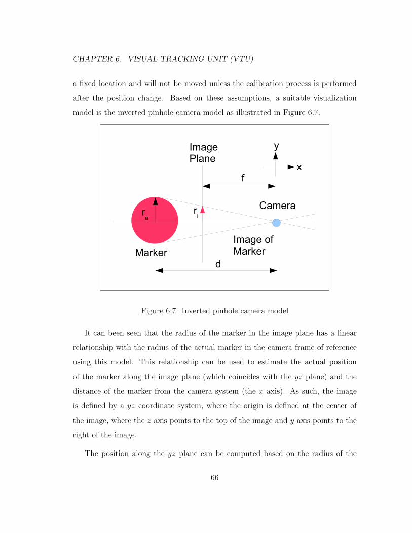
CHAPTER 6. VISUAL TRACKING UNIT (VTU)
a fixed location and will not be moved unless the calibration process is performed
after the position change. Based on these assumptions, a suitable visualization
model is the inverted pinhole camera model as illustrated in Figure 6.7.
Image of MarkerMarker
ImagePlane
Camerarir
a
f
d
y
x
Figure 6.7: Inverted pinhole camera model
It can been seen that the radius of the marker in the image plane has a linear
relationship with the radius of the actual marker in the camera frame of reference
using this model. This relationship can be used to estimate the actual position
of the marker along the image plane (which coincides with the yz plane) and the
distance of the marker from the camera system (the x axis). As such, the image
is defined by a yz coordinate system, where the origin is defined at the center of
the image, where the z axis points to the top of the image and y axis points to the
right of the image.
The position along the yz plane can be computed based on the radius of the
66

CHAPTER 6. VISUAL TRACKING UNIT (VTU)
marker and that of the marker in the image plane using the following equation:
ya = (ra/ri,p)yi (6.3)
za = (ra/ri,p)zi (6.4)
where (ya, za) are the actual yz coordinates in the camera frame of reference, and
(yi, zi) are the coordinates in the image plane, ra is the actual radius of the marker,
and ri,p is the radius of the marker in the image plane in pixels. The distance of
the marker from the camera system can be computed using the following equation:
xa = −d = − f
ri
ra (6.5)
where xa is the x coordinate of the marker in the camera frame of reference, f is
the focal length, ra is the actual radius of the marker, and ri is the radius of the
marker in the image plane.
6.5 Experimental Results
To test the accuracy of the VTU, the marker was placed at different locations with
known 3D coordinates. The estimated 3D position computed by the VTU was then
compared to the reference 3D coordinates for each of the locations. A total of 10
test trials were conducted to analyse the overall 3D position estimation accuracy
of the VTU. Furthermore, the tests were performed sequentially without system
recalibration to observe the long-term stability of the system. Table 6.1 lists the
specifications of the camera used for testing purposes.
67

CHAPTER 6. VISUAL TRACKING UNIT (VTU)
Sensor Type Focal Length Video Resolution Pixel Width Frame RateCMOS 5 mm 640×480 6.0µm 30 FPS
Table 6.1: Specifications of the test camera system
A summary of the position estimation accuracy results is shown in Table 6.2.
It can be observed that the VTU is effective at estimating the 3D position of the
marker. The RMS error is reasonably small and sufficient for the proposed sys-
tem considering the low-end DV camera system being used for testing purposes.
Therefore, it is evident that the VTU is capable of producing accurate results in
long-term scenarios. This is particularly important for the purpose of complement-
ing the INU system to produce 3D position information with improved accuracy
and stability.
Test Type RMS Error (cm) Error Standard Deviation (cm)ya, za coordinates 0.1590 0.1210xa coordinates 0.5103 0.1516
Table 6.2: Summary of VTU position accuracy test
68

Chapter 7
Vision-Inertial Fusion Unit
(VIFU)
This chapter describes in detail the overall design of the vision-inertial fusion unit
(VIFU). The first section presents an introduction to sensor data fusion. The
underlying theory behind two different sensor fusion techniques (complementary
filters and Kalman filters) are described in Section 7.2. Section 7.3 provides a
structural overview of the VIFU. Finally, Section 7.4 presents the error model used
in the error-state complementary Kalman filter of the VIFU.
7.1 Introduction
Sensor data fusion is the process of combining sensory data from multiple, different
sensor acquisition sources. The sensor sources can be composed of homogeneous
sensors (i.e., a sensor network of cameras) or heterogeneous sensors (i.e., cameras
69

CHAPTER 7. VISION-INERTIAL FUSION UNIT (VIFU)
coupled with accelerometers). There are a number of different reasons for perform-
ing sensor data fusion.
First, sensor data fusion may be performed to produce information that is more
accurate and detailed than possible using a single sensor device. For example,
sensor readings from a highly accurate but low frequency sensor can be combined
with sensor readings from a less accurate but high frequency sensor to produce
accurate and detailed sensor readings.
Another reason for sensor data fusion is to produce information that provides a
more complete picture of the environment than can be obtained a single sensor. For
example, multiple sensors can placed to observe non-overlapping regions spatially
or temporally to acquire different sensor readings on a particular scene. One prac-
tical application of this approach is image super-resolution where data acquired by
multiple cameras placed at different positions is combined to produce an image at
a higher resolution than that of any individual camera. Finally, sensor data fusion
may be performed to improve the robustness of the system against individual sensor
failures. This is useful in scenarios where one or more sensors in a sensor network
may fail due to environmental or technical circumstances. One practical application
for this approach is wide area environment monitoring, where many low-cost sensors
are deployed to ensure adequate sensor readings. This is particularly important in
hazardous environments where sensors are prone to failure.
Sensor fusion may be divided into three general classes [Kov01]: i) comple-
mentary, ii) cooperative, and iii) competitive. In complementary sensor fusion,
individual sensors either acquire sensor readings on different (adjacent) environ-
ments or contribute sensor readings on different aspects of the same environment.
Sensor readings acquired by individual sensors for the purpose of complementary
70

CHAPTER 7. VISION-INERTIAL FUSION UNIT (VIFU)
sensor fusion often have little or no overlap and can be combined to create a more
complete picture of the environment. In general, complementary sensor fusion does
not yield new information that cannot be measured directly by one or more of the
individual sensors.
In cooperative sensor fusion, sensor data from individual sensors are used to
produce new information that cannot be measured directly by an individual sensor.
An example of this is stereoscopic sensor fusion which takes 2D images acquired by
cameras at different viewpoints to produce a 3D representation of the environment.
The 3D information cannot be measured directly by any one of the individual
cameras.
Finally, competitive sensor fusion makes use of equivalent information about the
environment from individual sensors. This is typically used to provide redundancy
in case of individual sensor device failures. This technique can also be used to
improve the reliability of the sensor results.
The VIFU in the proposed system is a complementary sensor fusion system that
combines data obtained from heterogenous sensors (inertial and visual sensors).
While the accelerometer sensors can acquire information at a very high sampling
rate to produce a very detailed picture of the motion of the wireless 3D controller,
they are unable to maintain long-term accuracy due to rapid error accumulation.
On the other hand, the visual sensor system is capable of maintaining long-term
accuracy but can only acquire information at a low sampling rate due to technical
and computational limitations. Therefore, the VIFU exploits the advantages of
each of these sensor types to produce 3D position data that provides greater detail
than that possible with the visual sensor system and greater long-term stability
than can be achieved using only the inertial sensor system.
71

CHAPTER 7. VISION-INERTIAL FUSION UNIT (VIFU)
7.2 Sensor Fusion Techniques
The first step to designing the VIFU for the proposed system is to determine the
sensory fusion technique to be used. Two of the most widely used techniques for
sensor fusion are: i) complementary filters, and ii) Kalman filters.
7.2.1 Complementary Filters
There are many situations where sensors with different noise and frequency charac-
teristics are used to to measure the same physical phenomenon at the same time. It
is often the case by design that one sensor source provides higher sensitivity and/or
less noise at one frequency band while another sensor source provides higher sen-
sitivty and/or less noise at another frequency band. For example, a camera sensor
device provides better sensory data at low frequencies while an inertial sensor de-
vice provides better data at high frequencies. Therefore, it is desirable to combine
the low frequency characteristics of the camera system and the high frequency
characteristics of the inertial sensor.
This can be achieved through the use of a complementary filter system. A
complementary filter system is a pair of filters whose transfer functions add up to
one at all frequencies [WHL04]. A typical complementary filter system is composed
of a low pass filter, a high pass filter, and a combiner. In the case of a heterogenous
sensor system consisting of a visual sensor system and an inertial sensor system,
the data from the visual sensor system is filtered by a low-pass filter and the data
from the inertial sensor system is filtered by a high-pass filter. The two filtered data
signals are then summed up by the combiner to produce a final output signal. This
process is illustrated in Figure 7.1. One of the main advantages of a complementary
72

CHAPTER 7. VISION-INERTIAL FUSION UNIT (VIFU)
filter system is that it is relatively simple to implement. However, it does not take
into account error sources such as bias errors.
Inertial SensorSystem
Visual SensorSystem
High pass filter
Low pass filter
+Final outputsignal
Figure 7.1: Complementary filter system
7.2.2 Kalman Filters
Another widely used technique for sensor fusion is the use of a Kalman filter [Kal60].
The Kalman filter is a recursive discrete data filter is used to perform state esti-
mation for dynamic systems. Kalman filters have been used extensively in a wide
range of fields, particularly in the area of navigation and control systems. These
filters are popular for a number of reasons. First, they are computationally efficient.
Second, they are very versatile and capable of providing good state estimates for
past time, present time, and future time. Finally, they are able to use dynamic
models and error models of the underlying system to effectively reduce the effects
of noise on the resulting state estimates. Therefore, a Kalman filter approach is
73
CHAPTER 7. VISION-INERTIAL FUSION UNIT (VIFU)
better suited than the complementary filter approach in situations where the sensor
data may be corrupted by noise.
Rather than explaining in detail the mathematical theory of Kalman filters, the
general implementation methodology is presented in context of inertial navigation
systems. The discrete Kalman filter can be seen as a series of equations that take
a state estimate from the previous time step and a measurement from the current
time step to determine an estimate of the current state of the dynamic system.
The Kalman filter makes use of a dynamic model and an observation model of
the system. The dynamic model can be generalized as follows (neglecting optional
control inputs):
xk = Axk−1 + wk−1 (7.1)
where x is the state of the system, k is the current time step, the matrix A is
the dynamic model that relates the state at the previous time step to that at the
current time step, and w represents the process noise. The observation model can
be generalized as:
zk = Hxk + vk (7.2)
where z is the measurement at a specific time step, H is the observation model
that relates the state of the system with the measurement, and v represents the
measurement noise. The measurement noise and the process noise are assumed to
be zero-mean, white, and normally distributed:
74

CHAPTER 7. VISION-INERTIAL FUSION UNIT (VIFU)
p(w) ∼ N(0, Q) (7.3)
p(v) ∼ N(0, R) (7.4)
where Q and R are the process noise covariance and the measurement noise co-
variance respectively. In the case of inertial data, the dynamic model consists of
a system of dynamic equations used to compute position/orientation, velocity, and
acceleration.
The Kalman filter is divided into a prediction step and an update step. The
first step is the prediction step which predicts the state at the current time step
based on an estimate of the previous time step. The prediction step is defined by
the following equations (neglecting optional control inputs):
x̂k|k−1 = Ax̂k−1|k−1 (7.5)
Pk|k−1 = APk−1|k−1ATk + Qk (7.6)
where x̂k|k−1 is an estimate at time step k using only knowledge about the process
at the previous time step, and Pk|k−1 is the error covariance at time step k using
knowledge about the process at the previous time step.
The second step of the Kalman filter process is the update step, which adjusts
the state estimate made in the prediction step using the measurement made at the
current time step such that mean squared error is minimized:
Kk = Pk|k−1HT (HPk|k−1H
T + R)−1 (7.7)
75

CHAPTER 7. VISION-INERTIAL FUSION UNIT (VIFU)
x̂k = x̂k|k−1 + Kk(zk −Hx̂k|k−1) (7.8)
Pk = (I−KkH)Pk|k−1 (7.9)
where K is the Kalman gain and I is the identity matrix. After the state and error
covariance has been estimated for the current time step, this can then be used to
make subsequent estimates at other time steps. A Kalman filter based approach
is used in the proposed system because of its ability to handle noisy sensor data.
This is particularly important for the inertial sensors used in the proposed system
since these sensors provide measurements that can be corrupted by various types
of measurement noise.
7.3 VIFU Structural Overview
The VIFU used in the proposed motion capture system is implemented as part of
the PC processing system. The general architecture of the VIFU is illustrated in
Figure 7.2. The 3D position information from the VTU and the INU are fed into an
error-state complementary Kalman filter system which fuses the sensor data from
both sources into a unified 3D position data output.
7.4 Error-State Complementary Kalman Filter
The VIFU is laid out into what is known as an error-state complementary Kalman
filter configuration [May79, CDW94]. This is illustrated in Figure 7.3. In this
configuration, the difference is calculated between the 3D position output from the
INU and from the VTU. Using the output of the VTU as the reference point, the
76

CHAPTER 7. VISION-INERTIAL FUSION UNIT (VIFU)
Figure 7.2: VIFU setup
difference represents the position error of the INU. This position error signal is then
used as the measurement signal to the Kalman Filter. In an error-state Kalman
complementary filter configuration, the classic Kalman filter is used to continually
estimate the error of the inertial sensor data. The error estimates are then used to
correct the inertial sensor data outputs of the INU. The advantage of using an error-
state complementary Kalman filter configuration is that the detailed information
from the INU data at high frequencies can be preserved while the errors in the low
frequencies can be corrected. This results in an output signal that is detailed and
maintains long-term reliability.
Since the Kalman filter is used to provide an error estimate for the inertial sensor
data from the INU, it is necessary to establish an error model and observation model
for the system. Since the constant bias error in the inertial sensor data has been
corrected in the INU, the primary goal of the error-state complementary Kalman
77
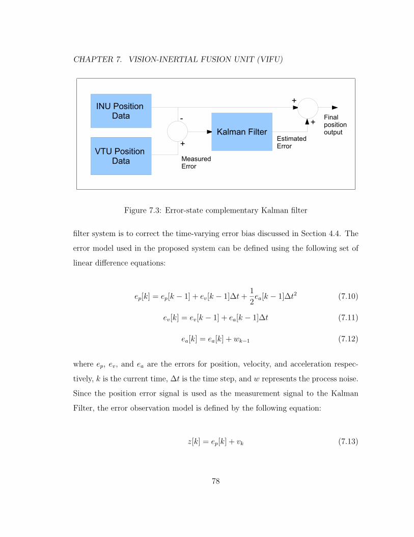
CHAPTER 7. VISION-INERTIAL FUSION UNIT (VIFU)
INU Position Data
VTU Position Data
+
+Kalman Filter
+- Final position output
EstimatedError
Measured Error
Figure 7.3: Error-state complementary Kalman filter
filter system is to correct the time-varying error bias discussed in Section 4.4. The
error model used in the proposed system can be defined using the following set of
linear difference equations:
ep[k] = ep[k − 1] + ev[k − 1]∆t +1
2ea[k − 1]∆t2 (7.10)
ev[k] = ev[k − 1] + ea[k − 1]∆t (7.11)
ea[k] = ea[k] + wk−1 (7.12)
where ep, ev, and ea are the errors for position, velocity, and acceleration respec-
tively, k is the current time, ∆t is the time step, and w represents the process noise.
Since the position error signal is used as the measurement signal to the Kalman
Filter, the error observation model is defined by the following equation:
z[k] = ep[k] + vk (7.13)
78

CHAPTER 7. VISION-INERTIAL FUSION UNIT (VIFU)
where z is the measured position error at a specific time step and v represents the
measurement noise.
Based on the above error model and observation model, the Kalman filter state
space matrices are given by:
A =
1 ∆t 1
2∆t2
0 1 ∆t
0 0 1
(7.14)
HVTUOn=
[1 0 0
](7.15)
HVTUOff=
[0 0 0
](7.16)
Q =
σ2
pnoise 0 0
0 σ2pnoise 0
0 0 σ2pnoise
(7.17)
R =[σ2
mnoise
](7.18)
where HVTUOnis the observation model matrix when data is available from the
VTU, HVTUOffis the observation model matrix when data is not available from
the VTU, σ2pnoise is the process noise variance and σ2
mnoise is the measurement noise
variance.
To test the effectiveness of the error-state complementary Kalman filter, the
79

CHAPTER 7. VISION-INERTIAL FUSION UNIT (VIFU)
position accuracy tests introduced in Chapter 4 were performed on the enhanced
system. For the purpose of the tests, the wireless 3D controller was left in a
fixed location with no external forces being exerted on the device. The VTU was
configured such that position information was available to the VIFU at a sampling
rate of 2 samples/second. This enabled an investigation of the effectiveness of
the system with visual data available at a very low frequency. Such a scenario is
common for consumer-level devices and applications. The results of the position
accuracy tests are presented in Table 7.1.
Original Results Filtered ResultsTest No. Mean Error Mean Error
Accumulated Standard Accumulated StandardError (m) Deviation (m) Error (m) Deviation (m)
1 0.156 0.0112 0.00287 0.00172 1.540 0.1784 0.00355 0.00183 2.6885 0.4014 0.00383 0.00254 8.0794 0.7622 0.01087 0.0020
Table 7.1: Summary of position accuracy tests
A graph illustrating the position error for the x channel for a time period of
63.96 s with and without the error-state complementary Kalman filter is shown in
Figure 7.4. It can be observed that filtering significantly reduces the position error.
Furthermore, the position error after filtering remains consistent and stable over
the entire measurement time period. Therefore, it is evident that the error-state
complementary Kalman filter can be used effectively to fuse information from the
VTU and the INU into a 3D position output that is both detailed and reliable over
time.
80

CHAPTER 7. VISION-INERTIAL FUSION UNIT (VIFU)
Figure 7.4: Position error over time for error-state complementary Kalman filter
81

Chapter 8
Conclusions
A vision-inertial motion capture system for wireless 3D controllers is capable of
providing detailed and reliable 3D position and orientation information using only
low-cost inertial sensors and visual sensors. Inertial tracking systems using ac-
celerometers and gyro sensors provide accurate high frequency motion readings but
suffer from rapid error accumulation. Visual tracking systems using one or more
cameras provide accurate motion readings at low frequencies but high frequency
motion readings are not possible due to the relatively high processing demands of
object detection. By transforming the inertial data to coincide with the visual data,
the sensor data from the two types of sensors can be fused to provide better 3D
position readings than otherwise possible using either a visual tracking system or
an inertial tracking system alone.
82

CHAPTER 8. CONCLUSIONS
8.1 Thesis Contributions
The thesis dissertation presents a design study on a visual-inertial motion cap-
ture system for wireless 3D controllers. The results of this study demonstrate the
feasibility of such a device for consumer-level applications. This thesis provides a
foundation for future research in consumer-level hybrid motion capture systems for
human computer interfaces by making several contributions. The primary contri-
butions of the dissertation include:
• describes the design of a visual-inertial hybrid motion capture system using
low-cost sensor components,
• provides experimental results demonstrating the error accumulation of inertial
devices when used to derive 3D position information,
• describes calibration methods for synchronizing inertial sensor data with vi-
sual sensor data,
• provides experimental results demonstrating the effectiveness of combining
colour thresholding, a circular Hough transform, and distance measurement
using a pinhole camera model to visually track an object in 3D space in a
computationally efficient manner, and
• provides experimental results demonstrating the effectiveness of the error-
state complementary Kalman filter in producing better 3D position by fusing
visual sensor data with inertial sensor data.
The secondary contributions of the dissertation include:
83

CHAPTER 8. CONCLUSIONS
• introduces and explains the concepts associated with the design of motion
capture systems, and
• presents several of the challenges associated with the design of a low-cost
hybrid motion capture system.
8.2 Potential for Future Research
The research presented in this dissertation provides a foundation for future research
in consumer-level hybrid motion capture systems. Two potential research topics
that can build upon the research presented in this dissertation are the following:
• low-cost multi-marker visual-inertial motion capture systems, and
• mainstream software applications utilizing motion capture.
8.2.1 Low-Cost Multi-Marker Visual-Inertial Motion Cap-
ture
For the purpose of this research, a motion capture system was designed for tracking
a single wireless 3D controller. As the device has no moveable parts, a single marker
was tracked by the proposed system. Future research could expand the system to
track multiple markers placed on a device with moveable parts and/or a user’s body
while still utilizing low-cost sensor devices. This research could lead to a number of
different consumer-level applications such as low-cost motion capture systems for
small animation studios and consumer-level interactive video games where virtual
84

CHAPTER 8. CONCLUSIONS
objects are manipulated in real-time using hand motion. An investigation of the
feasibility of building such a device using low-cost components is recommended.
8.2.2 Mainstream Software Applications Utilizing Motion
Capture
The objective of the research presented in this thesis is the design of the actual
motion capture system used to track a wireless 3D controller. However, such a
system would not be useful without mainstream software applications that can
utilize it to its full potential. Current mainstream software applications that can
make use of the proposed system include writing and drawing tools as well as 3D
modeling tools. However, these applications are not designed around such a system
and therefore do not take full advantage of the level of freedom and interactivity
the proposed system can deliver. Therefore, an investigation into possible future
mainstream software applications that can truly take advantage of the proposed
system is recommended.
8.3 Thesis Applicability
The work presented in this thesis has provided a practical solution to motion capture
using wireless 3D controllers. Experimental results show that it is possible to
implement the proposed system using low-cost visual and inertial sensor devices.
Therefore, the proposed system is well-suited for consumer-level applications that
can utilize motion-based input from a user, such as virtual reality systems, video
games, and motion capture for character animation.
85

Bibliography
[ADBW02] J. Gorman A. Duwel, M. Weinstein, J. Borenstein, and P. Ward.Quality factors of MEMS gyros and the role of thermoelastic damping.In Proceedings of The Fifteenth IEEE International Conference onMicro Electro Mechanical Systems, pages 214–219, 2002.
[Ani06] Gypsy5 Mechanical Motion Capture. World Wide Web Document,October 2006. http://www.animazoo.com/products/gypsy5.htm.
[Asc06] MotionStar. World Wide Web Document, October 2006. http://
www.ascension-tech.com/products/motionstar.php.
[BGS+05] P. Bruyant, M. Gennert, G. Speckert, R. Beach, J. Morgenstern, N.Kumar, S. Nadella, and M. King. A Robust Visual Tracking Systemfor patient motion. IEEE Transaction on Nuclear Science, 52(5):1288–1294, October 2005.
[Blo06] J. Blomster. Orientation estimation combining vision and gyro mea-surements. Master’s thesis, Royal Institute of Technology, April 2006.
[Boy05] J. Boyd. Good Vibrations from Epsons New Gyro-Sensor. TechnologyNewsline, 12, February 2005.
[Bre77] J. Bresenham. A linear algorithm for incremental digital display ofcircular arcs. Communications of the ACM, 20(2):100–106, 1977.
[CDW94] S. Cooper and H. Durrant Whyte. A frequency response method formulti-sensor high-speed navigation systems. In Proceedings of IEEEInternational Conference on Multisensor Fusion and Integration forIntelligent Systems, pages 1–8, October 1994.
86

BIBLIOGRAPHY
[CJD03] Y. Caritu C. Joguet and D. David. ’Pen-like’ natural graphic gesturecapture disposal, based on a micro-system. In Smart Objects Confer-ence, May 2003.
[DGEE03] J. Powell D. Gebre Egziabher, C. Lee Boyce Jr. and P. Enge. AnInexpensive DME-Aided Dead Reckoning Navigator. Navigation,50(4):247–264, Winter 2003.
[DH72] R. Duda and P. Hart. Use of the Hough Transform to detect lines andcurves in pictures. Communications of the ACM archive, 15(1):11–15,January 1972.
[EFGP98] M. Harrington E. Foxlin and George Pfeifer. Constellation: A wide-range wireless motion-tracking system for augmented reality and vir-tual set application. In Proceedings of SIGGRAPH 98, pages 371–378,1998.
[Eye06] Eyetoy. World Wide Web Document, October 2006. http://www.
eyetoy.com.
[FN03a] E. Foxlin and L. Naimark. Miniaturization, calibration & accuracyevaluation of a hybrid self-tracker. In Proceedings of the 2nd IEEEand ACM International Symposium on Mixed and Augmented Reality,pages 151–160, Washington, DC, USA, 2003. IEEE Computer Society.
[FN03b] E. Foxlin and L. Naimark. Vis-tracker: A wearable vision-inertialself-tracker. In Proceedings of IEEE Virtual Reality, pages 199–206,March 2003.
[GE04] D. Gebre Egziabher. Design and Performance Analysis of A Low-costAided Dead Reckoning Navigator. PhD thesis, Stanford University,February 2004.
[HSV06] HSV color space. World Wide Web Document, October 2006. http:
//en.wikipedia.org/wiki/HSV_color_space.
[Int07] InterSense Wireless InertiaCube3. World Wide Web Document,March 2007. http://www.isense.com/uploadedFiles/Products/
WirelessInertiaCube3.pdf.
[JLA95] J. Dias J. Lobo, P. Lucas and A. Almeida. Inertial Navigation Systemfor Mobile Land Vehicles. In Proceedings of ISIE95, pages 843–848,1995.
87

BIBLIOGRAPHY
[JOH00] G. Brostow J. O’Brien, B. Bodenheimer and J. Hodgins. AutomaticJoint Parameter Estimation from Magnetic Motion Capture Data. InProceedings of Graphics Interface 2000, pages 53–60, May 2000.
[Kal60] R. Kalman. A New Approach to Linear filtering and prediction prob-lems. Transaction of the ASME-Journal of Basic Engineering, pages35–45, March 1960.
[KD04] G. Klein and T. Drummond. Tightly integrated sensor fusion forrobust visual tracking. Image and Vision Computing, 22(10):769–776,September 2004.
[KGK02] J. Junkins K. Gunnam, D. Hughes and N. Kehtornavaz. A DSP em-bedded optical navigation system. In Proceedings of the 6th Interna-tional Conference on Signal Processing, volume 2, pages 1735–1739,2002.
[Kio06] Kionix. World Wide Web Document, October 2006. http://www.
kionix.com/.
[Kov01] V. Koval. The competitive sensor fusion algorithm for multi sensor sys-tems. In International Workshop on Intelligent Data Acquisition andAdvanced Computing Systems: Technology and Applications, pages65–68, July 2001.
[Lui02] H. Luinge. Inertial Sensing of Human Movement. PhD Dissertation,University of Twente, December 2002.
[May79] P. Maybeck. Stochastic Models, Estimation and Control, volume I.Academic Press, New York, 1979.
[Mic07] G-Link 2.4GHz Wireless Accelerometer Product Datasheet. WorldWide Web Document, March 2007. http://www.microstrain.com/
product_datasheets/2400_g-link_datasheet.pdf.
[MJVR03] J. Mulder, J. Jansen, and A. Van Rhijn. An affordable optical headtracking system for desktop vr/ar systems. In Proceedings of the work-shop on Virtual environments 2003, pages 215–223, 2003.
[MLCVA00] S. Sclaroff M. La Cascia and Vassilis Athitsos. Fast, reliable headtracking under varying illumination: An approach based on regis-tration of texture-mapped 3d models. IEEE Transaction on PatternAnalysis and Machine Intelligence, pages 322–336, April 2000.
88

BIBLIOGRAPHY
[NDI06] NDI. World Wide Web Document, October 2006. http://www.
ndigital.com/.
[Pha06] Phasespace. World Wide Web Document, October 2006. http://
www.phasespace.com/.
[RLG+02] M. Ribo, P. Lang, H. Ganster, M. Brandner, C. Stock, and A.Pinz. Hybrid tracking for outdoor augmented reality applications.IEEE Computer Graphics and Applications, 22(6):54–63, Novem-ber/December 2002.
[Roe06] D. Roetenberg. Inertial and Magnetic Sensing of Human Motion. PhDDissertation, University of Twente, May 2006.
[Sch06] A. Schumacher. Integration of a gps aided strapdown inertial navi-gation system for land vehicles. Master’s Thesis, Royal Institute ofTechnology, March 2006.
[SH05] I. Skog and P. Handel. A Low-cost gps aided inertial navigation systemfor vehicle applications. In Proceedings of the Thirdteenth EuropeanSignal Processing Conference, September 2005.
[SYA99] U. Neumann S. You and R. Azuma. Hybrid inertial and vision trackingfor augmented reality registration. In Proceedings of IEEE VirtualReality, pages 260–267, March 1999.
[SZM03] R. Chellappa S. Zhou and B. Moghaddam. Adaptive Visual Trackingand Recognition using Particle Filters. In Proceedings of IEEE In-ternational Conference on Multimedia and Expo, pages 349–352, July2003.
[Vic06] Vicon. World Wide Web Document, October 2006. http://www.
vicon.com.
[VKS06] S. Vogtl, A. Khamenel, and F. Saueri. Reality augmentation for med-ical procedures: System architecture, single camera marker tracking,and system evaluation. International Journal of Computer Vision,70(2):179–190, November 2006.
[WHL04] C. Hardham W. Hua, D. DeBra and B. Lantz. Polyphase FIR comple-mentary filters for control systems. In Proceedings of Spring TopicalMeeting on Control of Precision Systems, pages 109–114, April 2004.
89

BIBLIOGRAPHY
[Wii06] Wii. World Wide Web Document, October 2006. http://www.wii.
com.
[YAG+03] S. Yu, C. Allen, D. Geng, D. Burn, U. Brechany, G. Bell, and R. Row-land. 3-D motion system (data-gloves): application for parkinson’sdisease. IEEE Transactions on Instrumentation and Measurement,52(3):662–674, June 2003.
90