Lossless Compression of Volumetric Medical Images with Improved 3-D SPIHT Algorithm

Sungdae Cho*, Dongyoun Kim**, and William A. Pearlman*

*Center for Image Processing Research

Dept. Electrical, Computer and Systems Engineering

Rensselaer Polytechnic Institute

110 Eighth Street

Troy, NY 12180-3590

**Medical Image Processing Lab.

Dept. of Biomedical Engineering

Yonsei University,

220-710 Maji 234, Heungup

Wonjoo, Kangwon, Korea

Corresponding Author :

Prof. William A. Pearlman

Tel: 518-276-6082

Fax: 518-276-8715

E-mail: pearlman@rpi.edu

Abstract This paper presents a lossless compression of volumetric medical images with the improved 3-D SPIHT algorithm that searches on asymmetric trees. The tree structure links wavelet coefficients produced by three-dimensional reversible integer wavelet transforms. Experiments show that the lossless compression with the improved 3-D SPIHT gives improvement about 42% on average over two-dimensional techniques, and is superior to those of prior results of three-dimensional techniques. In addition to that, we can easily apply different numbers of decompositions between the transaxial and axial dimensions, which is a desirable function when the coding unit of a group of slices is limited in size.

Keywords asymmetric tree structure, SPIHT, 3-D wavelet transform, lossless compression.

INTRODUCTION

Digital technology has given a great advantage to the medical imaging area. Medical images, however, require huge amounts of memory, especially volumetric medical images, such as computed tomography (CT), and magnetic resonance (MR) images. Due to the limitations of storage and transmission bandwidth of the images, the main problem of the technology lies in how to compress a huge amount of visual data into a low bitrate stream, because the amount of medical image data would overwhelm the storage device without an efficient compression scheme.

Compression schemes can be generally classified into two schemes : lossless and lossy compression. Lossy compression usually provides much higher compression than lossless compression, because the reconstructed image is not exactly the same as the original image. Although lossy compression is generally acceptable for image browsing, lossless compression of medical image data has been required by doctors for accurate diagnosis and legal protection, because lossless compression allows exact recovery of the original image.

Volumetric medical images are a three-dimensional (3-D) image data set, and can be

considered as a sequence of two-dimensional (2-D) images, or slices. A simple way is to directly apply a two dimensional compression algorithm to each slice independently. However, the slices are generally highly correlated with one another, so a transform is used to decorrelate the data and to improve performance of compression. Therefore, the 3-D based approaches could provide better compression results. In 3-D approach, contiguous groups of slices (GOS) are coded, and the small GOS sizes are desirable for random access to certain segments of slices

The embedded zero-tree wavelet (EZW) [1] coding algorithm was introduced by

Shapiro with excellent compression results. Later, Said and Pearlman proposed a more efficient coding algorithm using set partitioning in hierarchical tree (SPIHT), and implemented to both lossy [2] and lossless [3] compression of images. B. Kim and Pearlman [4] extended 2-D to 3-D for video, and Y. Kim and Pearlman [5] utilized it for volume image compression.

In this paper, we use Kim and Pearlman's [5] lossless 3-D SPIHT with asymmetric

tree structure. Our experiments demonstrate that the lossless compression of asymmetric tree 3-D SPIHT (AT-SPIHT) algorithm outperforms the symmetric tree 3-D SPIHT. In addition to that, we show that the AT-SPIHT gives flexibility of choosing the GOS size and decomposition levels, and gives excellent results for small GOS sizes.

METERIALS AND METHODS

A. Asymmetric Tree Structure of 3-D SPIHT In previous work, Kim et al. [5] have used the 3-D SPIHT compression kernel with

the tree structure introduced in [6]. This tree structure is just a simple extension of the symmetric 2-D SPIHT tree structure. Other researchers have proposed a more efficient tree structure [7][8]. The 3-D SPIHT algorithm is one of the tree based coders, and the tree-based coders tend to give better performance when tree depth is long and the statistical distribution of magnitudes of wavelet coefficients is uneven between the intra-slice and inter-slice directions. Therefore, the main idea of this tree structure is to make the trees longer, since that increases the probability of a coefficient value being zero as we move from root to leaves. To make that kind of tree, we can simply decompose into more levels and change the linkage of coefficients. We can not always decompose to more levels, since there is a limitation according to the image size and Group of Slice (GOS) size. On the other hand, the asymmetric tree structure always gives a longer tree than that of the normal 3-D SPIHT.

Figure 1 portrays the tree structures among the original 2-D tree structure after 2-level spatial decompositions, the original 3-D tree structure after 2-level wavelet packet decompositions, and the 3-D asymmetric tree structure after 2-level wavelet packet decompositions. To form trees of 2-D SPIHT as shown in Fig. 1 (a), groups of 2×2 coordinates were kept together in the lists. On the 3-D subband structure in Fig. 1 (b), there are 3-D transaxial and axial trees, and their parent-offspring relationships. To apply wavelet packet decomposition, the full axial decomposition precedes the transaxial decompositions, where the node divides in the additionally split subbands. The symmetric tree structure of 3-D SPIHT is a straightforward extension from the 2D case to form a node in 3-D SPIHT as a block of eight adjacent pixels with two extending to each of the three dimensions, hence forming a node of 2×2×2 pixels. The asymmetric tree structure shown in Fig. 1 (c) in each coefficient frame is exactly the same as the 2-D SPIHT tree structure except that the top-left coefficient of each 2×2 group in the lowest transaxial subband of LLt and LHt bands links to a group in another axial subband at the same transaxial subband location.

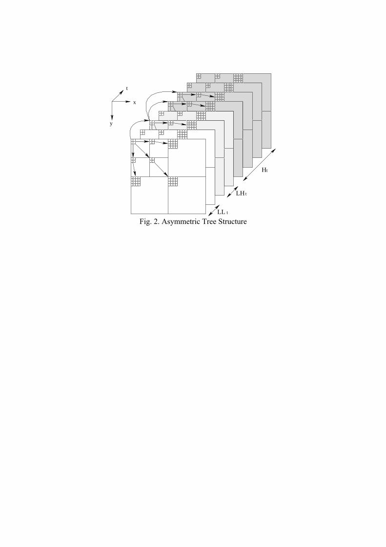
Figure 2 shows another view of the asymmetric tree structure. In this figure, there are eight frames, which are transformed in both the transaxial and axial domains in two levels. As we can see, the new tree structure has 2×2 wavelet coefficients element in axial root subband (LLt) rather than 2×2×2 wavelet coefficients element.

In 2-D SPIHT, the top left coefficient of each 2×2 group in the lowest subband is not part of any tree. On the other hand, the top-left coefficient of each 2×2 group in the

lowest transaxial subband in the asymmetric tree structure is linked with the 2×2 offspring group in the same transaxial location of the following axial subband except the highest axial subband. This means that the three coefficients of 2×2 group are linked with the 2×2 offspring group in the same coefficient frame, and one in another frame. As we can see in Figure 2, the top-left coefficient of each 2×2 group in the lowest transaxial subband of axial LLt band has one 2×2 offspring group in the axial LHt band, and the top-left coefficient of each 2×2 offspring group in the lowest transaxial subband of axial LHt band has two 2×2 offspring group in axial Ht band. This means that the top-left coefficients in LLt and LHt band are linked with the coefficients, which represent the same transaxial location in the following axial subband. Therefore, the top-left coefficient of each 2×2 offspring group in the lowest transaxial subband of axial Ht band does not have any offspring, because there are no more axial subbands. In this manner, the first stage of the tree is constructed. These are shown in Figure 2 by the arrows. To grow the tree further, each coefficient group is linked with each transaxial subband, the same as with original 2-D SPIHT. Therefore, each 2×2 coefficient group in the lowest transaxial subband of axial LLt band has three 2×2 offspring groups in axial LLt and one 2×2 offspring group in the LHt band, and each 2×2 offspring group in the lowest transaxial subband of axial LHt band has three 2×2 offspring groups in axial LHt and two in the Ht band. Each 2×2 offspring group in the lowest transaxial subband of axial Ht band has three 2×2 offspring groups in the same axial Ht band, because it is the highest frequency subband.

One potential advantage over the original symmetric tree structure is that it can be more easily applied to a different number of decompositions between the transaxial and axial dimensions, because this tree structure is naturally unbalanced. This function is very useful when the frame size is big and axial decomposition levels are limited. In that case, we can decompose to more levels in the transaxial domain than the axial domain. More transaxial decompositions usually produce noticeable coding gain. The tree structure of this different number of decompositions can be easily extended. For higher number of axial decompositions, the tree structure can be also extended. Kim et al. also used an unbalanced tree structure in [6], but it was more difficult to apply.

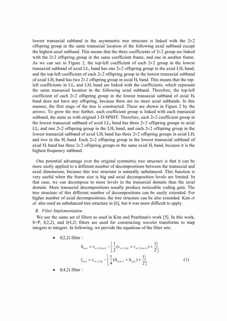
B. Filter Implementation We use the same set of filters as used in Kim and Pearlman's work [5]. In this work,

S+P, I(2,2), and I(4,2) filters are used for constructing wavelet transforms to map integers to integers. In following, we provide the equations of the filter sets.

• I(2,2) filter :

++−= +−−+− 2

1)(21

22,12,112,1, mnmnmnnm ccch

++−= −− 2

1)(41

,1,2,1, mnmnmnnm hhcl (1)

• I(4,2) filter :

++

−+−=

+−−−

+−−

+−

21)(

161

)(169

42,122,1

22,12,1

12,1,

mnmn

mnmn

mnnm

cc

ccch

(2)

++−= −− 2

1)(41

,1,2,1, mnmnmnnm hhcl

• S+P filter : h mnmnnm cc 2,112,1

1, −+− −=

+= −

1,2,1, 2

1nmmnnm hcl (3)

++−

+−+−=

++−−

−−−

21)()(

)()(

161

11,12,12,1

2,112,11

,,mnmnmn

mnmn

mnnm hcc

cch

γβ

αh

where denotes downward truncation. In Kim and Pearlman's work [5], the predictor parameters of S+P filter α = 3/16, β = 8/16, and γ= 6/16 were selected to get better performance for medical images.

⋅

RESULTS

We test the symmetric tree 3-D SPIHT and the asymmetric tree 3-D SPIHT (AT-

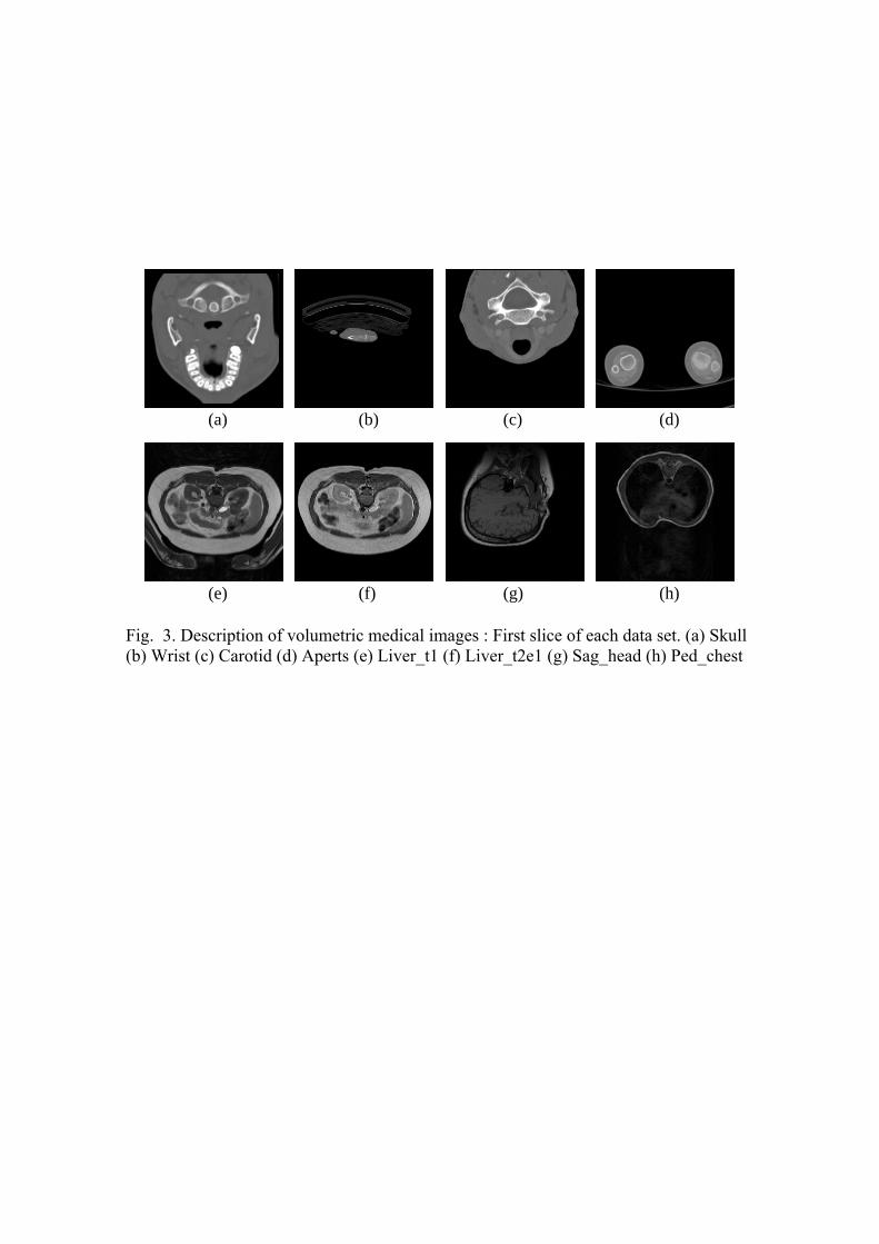
SPIHT) algorithms on the 8-bit CT and MR volumetric medical images used in Bilgin et al.'s work [9]. Table 1 shows the description of these images. The first slices of each data set are shown in Figure 3.

We first compare the performance of lossless compression with Group of Slice (GOS)

= 16 and 8 for 3 and 2 levels of decompositions, respectively, in both the axial and transaxial domains. Table 2 gives average lossless compression results in bpp (bits per pixel) using the symmetric tree 3-D SPIHT, and the AT-SPIHT with different filters (S+P, I(2,2), I(4,2)). To get the compression ratio in 8 bpp images, we can divide 8 by compression rate in bits per pixel (bpp). For I(4,2) filter, we apply the filter only to the transaxial domain, and use a shorter filter (e.g. I(2,2)) in the axial domain. As you can see, AT-SPIHT gives better performance than that of symmetric tree 3-D SPIHT except Carotid and Skull images when GOS=16. We also provide the bitrates of AT-SPIHT with higher GOS. To keep the 3 level decompositions, the symmetric tree structure 3-D SPIHT needs an even number of coefficient frames in the lowest axial subband to keep the 2×2×2 wavelet coefficients element in the band, but the AT-SPIHT does not have this limitation, because the tree structure uses a 2×2 wavelet coefficient element. This gives us flexibility in choosing the size of the GOS. For example, Aperts, Liver_t1, and Liver_t2 images have 48 slices. The symmetric tree structure 3-D SPIHT needs either 16 GOS or 48 GOS to have three level decompositions in the axial domain. However,

AT-SPIHT can use 16, 24, or 48 GOS with three level axial decompositions, so that we can flexibly choose the GOS according to the system memory.

In addition to the flexibility of choosing GOS, we can also choose many different levels of decompositions in the transaxial domain. As mentioned in the previous section, we can easily apply different numbers of decompositions between the transaxial and axial domains to the AT-SPIHT. This feature is highly desirable when GOS size is limited. To show the performance of different numbers of decompositions, we kept the same number of axial decomposition (two levels for GOS = 8), and used more level of transaxial decompositions. Table 3 shows the average bitrates with different number of decompositions when GOS = 8. We can see that the coding performance is improved as with more levels of decomposition in the transaxial domain, and beyond three of four levels of decomposition, the improvement is very small. In the case of the Aperts image, for example, the AT-SPIHT with GOS = 8 is better than symmetric tree 3-D SPIHT with GOS = 16 for more than 3 levels decomposition in the transaxial domain. For the other images, the bitrates of AT-SPIHT with GOS = 8 and higher levels of decomposition in the transaxial domain are comparable to those of the symmetric tree 3-D SPIHT with GOS = 16. This is an important feature of AT-SPIHT, since the efficient compression of small GOS allows easier and finer random access to a small number of slices.

Table 4 and 5 show the comparisons of lossless compression performance with other

compression algorithms. In these tables, all 3-D compression techniques use three level decompositions on the entire image volume. The reason for using the whole image volume as a GOS is to compare with other results [9][10]. We chose the I(4,2) filter for AT-SPIHT and 3-D SPIHT, because the filter gives the best results among the three filters (S+P, I(2,2), I(4,2)). The other 3-D compression techniques, such as 3-D EZW, 3-D CB-EZW, and Xiong's method, use I(2+2,2) integer filter, because this filter usually gives the best result with these compression algorithms. As we can see, AT-SPIHT performs better than 3-D SPIHT, with the single exception of the Carotid image. When we compare with other 3-D compression methods, AT-SPIHT still outperforms the other methods, except for the Cartoid and Aperts images with 3-D CB-EZW.

DISCUSSION

We showed a lossless compression of volumetric medical images with the asymmetric tree 3-D SPIHT (AT-SPIHT) algorithm. We presented our results by an approach that leads to wavelet transforms that map integers to integers, which can be used for lossless and lossy coding. The SPIHT algorithm with integer filters is fully embedded, the decoder, therefore, can stop the decoding process at any point of the bitstream and reconstruct the best quality of image at that bit rate. Furthermore, the AT-SPIHT can be more easily applied to a different number of decompositions between the transaxial and axial dimensions using naturally unbalanced characteristic of the tree structure.

For the different number of decompositions between the transaxial and axial

dimensions, we can expect coding gain as we decompose to more levels. When we

compare between 2-level and 6-level decompositions in transaxial dimension of I(4,2) filter with GOS size 8, there is about 2.4% improvement with 6 level decompositions.

For the effect of size of GOS on the performance of AT-SPIHT, a larger size GOS

gives better compression performance. When we compare between GOS of 8 and entire image volume, we can expect about 11% improvement, and beyond 16, get 4.4% improvement, and beyond 24, expect only 1.6% improvement in the case of the I(4,2) filter. However, as the GOS becomes larger, a larger size of memory is required and random access to segments of slices in the bitstream becomes coarser.

We saw that the AT-SPIHT performs much better than the methods that use

independent lossless coding of slices, because independent coding of slices does not exploit the inter-slice dependencies. Numerical results show that the compressed bitrates for the AT-SPIHT gives improvement about 42% on average compared with two-dimensional techniques. When we compare with the international standard of two-dimensional lossless compression technique (JPEG-LS), for example, AT-SPIHT improves compression by 28% on average. This results suggest that the three dimensional approach to compress the volumetric medical images should be used to exploit their inter-slice dependences.

CONCLUSION

In this paper, we have implemented the asymmetric tree structure to the 3-D SPIHT algorithm for lossless compression of volumetric medical data. In addition to the improvement over the symmetric tree 3-D SPIHT in terms of bitrates, one of the nice benefits of using asymmetric tree structure is the flexibility of choosing the size of GOS and the number of decomposition levels, because the number of decomposition levels in transaxial domain is totally independent from the number of decomposition levels in axial domain. Therefore, AT-SPIHT can be used when there are as few as 2 slices in a GOS. Furthermore, the 3-D SPIHT compression methods offer substantial decreases in bitrate over 2-D methods that encode each slice independently.

References

[1] Shapiro JM (1993), Embedded image coding using zerotrees of wavelet coefficient, IEEE Transactions on Signal Processing 41:3445-3462

[2] Said A, Pearlman WA (1996), A New, Fast and Efficient Image Codec Based on Set Partitioning in Hierarchical Trees, IEEE Transactions on CSVT 6:243-250

[3] Said A, Pearlman WA (1996), An image multiresolution representation for lossless and lossy compression, IEEE Transactions on Image Processing 5:1303-1010

[4] Kim B.-J, Pearlman WA (1997), An embedded wavelet video coder using three-dimensional set partitioning in hierarchical trees, Proceedings of DCC:251-260

[5] Kim YS, Pearlman WA (1999), Lossless Volumetric Image Compression, Proceedings of SPIE, Applications of Digital Image Processing XXII 3808:305-312

[6] Kim B.-J, Xiong Z, Pearlman WA (2000), Low bit-rate scalable video coding with 3-D SPIHT, IEEE Transactions on CSVT, 10:1374-1387

[7] Dragotti PL, Poggi G, Ragozini ARP (2000), Compression of multispectral images by 3-D SPIHT algorithm, IEEE Transactions on Geoscience and Remote Sensing 38:416-428

[8] He C, Dong J, Zheng YF, Gao Z (2003), Optimal 3-D Coefficient Tree Structure for 3-D Wavelet Video Coding, IEEE Transactions on CSVT, 13:961-972

[9] Bilgin A, Zweig G, Marcellin MW (2000), Three-dimensional image compression using integer wavelet packet transform, Applied Optics: Information Processing 39:1799-1814

[10] Xiong Z, Wu X, Yun DY (1998), Progressive coding of medical volumetric data using 3-D integer wavelet packet trasnsform, IEEE Workshop on Multimedia:553-558

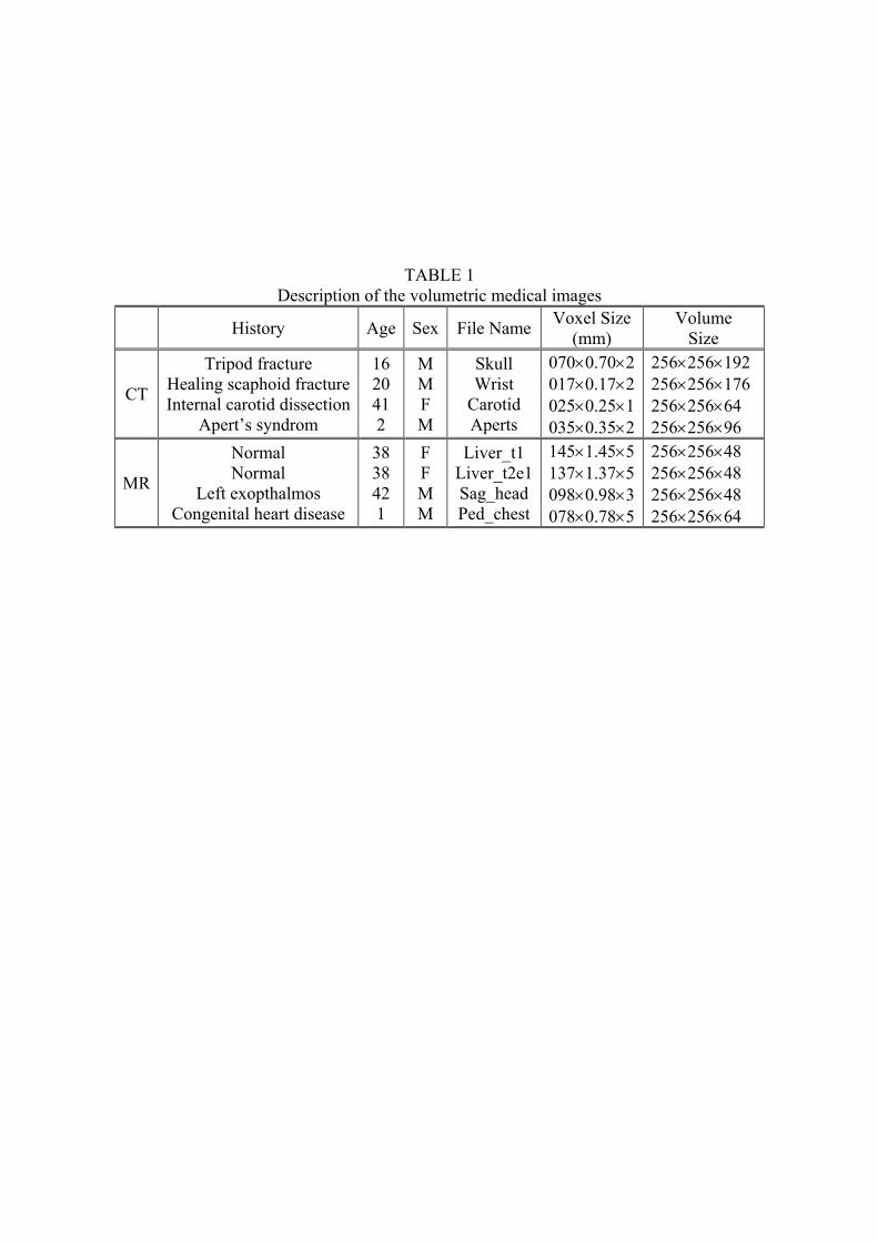
TABLE 1 Description of the volumetric medical images

History Age Sex File Name Voxel Size (mm)

Volume Size

CT

Tripod fracture Healing scaphoid fracture Internal carotid dissection

Apert’s syndrom

16 20 41 2

M M F M

Skull Wrist

Carotid Aperts

070×0.70×2 017×0.17×2 025×0.25×1 035×0.35×2

256×256×192 256×256×176 256×256×64 256×256×96

MR

Normal Normal

Left exopthalmos Congenital heart disease

38 38 42 1

F F M M

Liver_t1 Liver_t2e1 Sag_head Ped_chest

145×1.45×5 137×1.37×5 098×0.98×3 078×0.78×5

256×256×48 256×256×48 256×256×48 256×256×64

TABLE 2 Bitrates after lossless compression

3-D SPIHT AT-SPIHT GOS 8 16 8 16 24/32/88 48/64/176

Aperts

(8,16,24,48)

S+P I(2,2) I(4,2)

1.1197 1.0428 1.0250

1.0543 0.9738 0.9558

1.1020 1.0188 1.0028

1.0397 0.9522 0.9375

1.0345 0.9455 0.9300

1.0238 0.9285 0.9147

Carotid

(8,16,32.64)

S+P I(2,2) I(4,2)

1.5995 1.6066 1.5901

1.4977 1.5272 1.5115

1.5856 1.5942 1.5791

1.4973 1.5340 1.5192

1.4608 1.5075 1.4935

1.4500 1.4930 1.4790

Liver_t1

(8,16,24,48)

S+P I(2,2) I(4,2)

2.5428 2.4913 2.4580

2.3997 2.3573 2.3270

2.5045 2.4368 2.4058

2.3690 2.3120 2.2857

2.3355 2.2605 2.2365

2.3103 2.2300 2.2075

Liver_t2

(8,16,24,48)

S+P I(2,2) I(4,2)

1.8923 1.9035 1.8667

1.7483 1.7823 1.7500

1.8817 1.8632 1.8295

1.7440 1.7463 1.7170

1.7085 1.6940 1.6665

1.6850 1.6730 1.6461

Ped_chest

(8,16,32,64)

S+P I(2,2) I(4,2)

2.2000 1.9988 1.9134

2.1045 1.8105 1.7835

2.1576 1.9244 1.9104

2.0540 1.7650 1.7550

2.0310 1.6920 1.6835

2.0080 1.6570 1.6490

Sag_head

(8,16,24,48)

S+P I(2,2) I(4,2)

2.3468 2.1468 2.1422

2.2400 2.0563 2.0517

2.3108 2.1010 2.0965

2.2023 2.0060 2.0017

2.1795 1.9565 1.9530

2.1308 1.9300 1.9264

Skull

(8,16,32,64)

S+P I(2,2) I(4,2)

2.3210 2.3318 2.2980

2.1134 2.1081 2.0464

2.4483 2.3159 2.2976

2.1661 2.0399 2.0250

2.1108 1.9852 1.9708

2.0790 1.9583 1.9443

Wrist

(8,16,88,176)

S+P I(2,2) I(4,2)

1.4695 1.3758 1.3475

1.3689 1.2459 1.2231

1.4503 1.3430 1.3170

1.3550 1.2173 1.1976

1.3140 1.1445 1.1270

1.3090 1.1320 1.1150

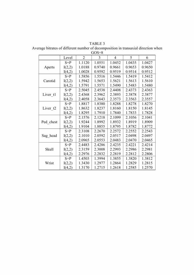
TABLE 3 Average bitrates of different number of decomposition in transaxial direction when

GOS=8 Level 2 3 4 5 6

Aperts

S+P I(2,2) I(4,2)

1.1120 1.0188 1.0028

1.0551 0.9740 0.9592

1.0452 0.9661 0.9519

1.0435 0.9653 0.9514

1.0427 0.9650 0.9512

Carotid

S+P I(2,2) I(4,2)

1.5856 1.5942 1.5791

1.5516 1.5653 1.5571

1.5446 1.5621 1.5490

1.5419 1.5613 1.5483

1.5412 1.5610 1.5480

Liver_t1

S+P I(2,2) I(4,2)

2.5045 2.4368 2.4058

2.4538 2.3962 2.3643

2.4408 2.3893 2.3573

2.4373 2.3878 2.3563

2.4363 2.3877 2.3557

Liver_t2

S+P I(2,2) I(4,2)

1.8817 1.8632 1.8295

1.8380 1.8237 1.7910

1.8288 1.8160 1.7840

1.8278 1.8150 1.7833

1.8270 1.8145 1.7828

Ped_chest

S+P I(2,2) I(4,2)

2.1576 1.9244 1.9104

2.1218 1.8992 1.8855

2.1099 1.8932 1.8795

2.1056 1.8919 1.8782

2.1041 1.8909 1.8772

Sag_head

S+P I(2,2) I(4,2)

2.3108 2.1010 2.0965

2.2670 2.0592 2.0553

2.2572 2.0517 2.0483

2.2552 2.0498 2.0470

2.2543 2.0497 2.0465

Skull

S+P I(2,2) I(4,2)

2.4483 2.3159 2.2976

2.4286 2.3008 2.2832

2.4235 2.2993 2.2819

2.4221 2.2986 2.2812

2.4214 2.2981 2.2806

Wrist

S+P I(2,2) I(4,2)

1.4503 1.3430 1.3170

1.3994 1.2977 1.2715

1.3855 1.2864 1.2618

1.3820 1.2829 1.2585

1.3812 1.2815 1.2570

TABLE 4 Comparison of different image compression methods on the CT data after three-level

decompositions of the whole dataset Method Skull Wrist Carotid Aperts

AT-SPIHT 1.9180 1.1150 1.4790 0.9090 3-D SPIHT 1.9550 1.1390 1.4680 0.9340 3-D EZW 2.2251 1.2828 1.5069 1.0024

3-D CB-EZW 2.0095 1.1393 1.3930 0.8923 Xiong 1.9950

JPEG-LS 2.8460 1.6531 1.7388 1.0637 JPEG2000 3.0877 1.7902 1.9896 1.2822 2-D SPIHT 2.6921 1.8378 1.9823 1.2330

CALIC 2.7250 1.6912 1.6547 1.0470 Gzip 3.8576 2.7751 2.8551 1.8243

UNIX Compress 4.1357 2.7204 2.7822 1.7399

LIST OF FIGURES

1. Comparison of tree structures (a) 2-D original tree structure after 2 level spatial decomposition (b) 3-D original tree structure after 2 level wavelet packet decomposition (c) 3-D asymmetric tree structure after 2 level wavelet packet decomposition

2. Asymmetric Tree Structure 3. Description of volumetric medical images: First slice of each data set. (a) Skull

(b) Wrist (c) Carotid (d) Aperts (e) Liver_t1 (f) Liver_t2e1 (g) Sag_head (h) Ped_chest

*

(a)

(b) (c)LL

LH

H

LL

LH

H

t

t

t

t

t

t

x

x

x

y

t t

y y

Fig. 1. Comparison of tree structures (a) 2-D original tree structure after 2 level spatial decomposition (b) 3-D original tree structure after 2 level wavelet packet decomposition (c) 3-D asymmetric tree structure after 2 level wavelet packet decomposition

LL

LH

H

x

y

t

t

t

t

Fig. 2. Asymmetric Tree Structure

(a) (b) (c) (d)

(e) (f) (g) (h)

Fig. 3. Description of volumetric medical images : First slice of each data set. (a) Skull (b) Wrist (c) Carotid (d) Aperts (e) Liver_t1 (f) Liver_t2e1 (g) Sag_head (h) Ped_chest