Data Compression for Maskless Lithography Systems: Architecture,Algorithms and Implementation

by

Vito Dai

B.S. (California Institute of Technology) 1998M.S. (University of California, Berkeley) 2000

A dissertation submitted in partial satisfaction of the

requirements for the degree of

Doctor of Philosophy

in

Department of Electrical Engineering and Computer Sciences

in the

GRADUATE DIVISION

of the

UNIVERSITY OF CALIFORNIA, BERKELEY

Committee in charge:Professor Avideh Zakhor, Chair

Professor Borivoje NikolicProfessor Stanley Klein

Spring 2008

The dissertation of Vito Dai is approved:

Chair Date

Date

Date

University of California, Berkeley

Spring 2008

Data Compression for Maskless Lithography Systems: Architecture,

Algorithms and Implementation

Copyright 2008

by

Vito Dai

1

Abstract

Data Compression for Maskless Lithography Systems: Architecture, Algorithms and

Implementation

by

Vito Dai

Doctor of Philosophy in Department of Electrical Engineering and Computer

Sciences

University of California, Berkeley

Professor Avideh Zakhor, Chair

Future lithography systems must produce more dense microchips with smaller

feature sizes, while maintaining throughput comparable to today’s optical lithogra-

phy systems. This places stringent data-handling requirements on the design of any

maskless lithography system. Today’s optical lithography systems transfer one layer

of data from the mask to the entire wafer in about sixty seconds. To achieve a similar

throughput for a direct-write maskless lithography system with a pixel size of 22 nm,

data rates of about 12 Tb/s are required. In this thesis, we propose a datapath ar-

chitecture for delivering such a data rate to a parallel array of writers. Our proposed

system achieves this data rate contingent on two assumptions: consistent 10 to 1

2

compression of lithography data, and implementation of real-time hardware decoder,

fabricated on a microchip together with a massively parallel array of lithography

writers, capable of decoding 12 Tb/s of data.

To address the compression efficiency problem, we explore a number of existing

binary and gray-pixel lossless compression algorithms and apply them to a variety

of microchip layers of typical circuits such as memory and control. The spectrum

of algorithms include industry standard image compression algorithms such as JBIG

and JPEG-LS, a wavelet based technique SPIHT, general file compression techniques

ZIP and BZIP2, and a simple list-of-rectangles representation RECT. In addition,

we develop a new technique, Context Copy Combinatorial Coding (C4), designed

specifically for microchip layer images, with a low-complexity decoder for application

to the datapath architecture. C4 combines the advantages of JBIG and ZIP, to achieve

compression ratios higher than existing techniques. We have also devised Block C4,

a variation of C4 with up to hundred times faster encoding times, with little or no

loss in compression efficiency.

The compression efficiency of various compression algorithms have been charac-

terized on a variety of layouts sampled from many industry sources. In particular, the

compression efficiency of Block C4, BZIP2, and ZIP is characterized for the Poly, Ac-

tive, Contact, Metal1, Via1, and Metal2 layers of a complete industry 65 nm layout.

Overall, we have found that compression efficiency varies significantly from design

to design, from layer to layer, and even within parts of the same layer. It is diffi-

3

cult, if not impossible, to guarantee a lossless 10 to 1 compression for all lithography

data, as desired in the design of our datapath architecture. Nonetheless, on the most

complex Metal1 layer of our 65 nm full chip microprocessor design, we show that a

average lossless compression of 5.2 is attainable, which corresponds to a throughput

of 60 wafer layers per hour for a 0.77 Tb/s board-to-chip communications link. As a

reference, state-of-the-art HyperTransport 3.0 offers 0.32 Tb/s per link. These num-

bers demonstrate the role lossless compression can play in the design of a maskless

lithography datapath.

The decoder for any chosen compression scheme must be replicated in hardware

tens of thousands of times, to achieve the 12 Tb/s decoding rate. As such, decoder

implementation complexity is a significant concern. We explore the tradeoff between

the compression ratio, and decoder buffer size for C4, which constitutes a significant

portion of the decoder implementation complexity. We show that for a fixed buffer

size, C4 achieves a significantly higher compression ratio than those of existing com-

pression algorithms. We also present a detailed functional block diagram of the C4

decoding algorithm as a first step towards a hardware realization.

Professor Avideh ZakhorDissertation Committee Chair

i

Contents

List of Figures iii

List of Tables v

1 Introduction 11.1 Microchip design and maskless lithography . . . . . . . . . . . . . . . 2

1.1.1 Data representation . . . . . . . . . . . . . . . . . . . . . . . . 101.2 Maskless Lithography System Architecture Designs . . . . . . . . . . 10

1.2.1 Direct-connection architecture . . . . . . . . . . . . . . . . . . 101.2.2 Memory architecture . . . . . . . . . . . . . . . . . . . . . . . 111.2.3 Compressed memory architecture . . . . . . . . . . . . . . . . 121.2.4 Off-chip compressed memory architecture . . . . . . . . . . . . 141.2.5 Off-chip compressed memory with on-chip decoding architecture 15

2 Data Compression Applied to Layer Data 202.1 Hierarchical flattening and rasterization . . . . . . . . . . . . . . . . . 212.2 Effect of rasterization parameters on compression . . . . . . . . . . . 232.3 Properties of layer images and their effect on compression . . . . . . . 282.4 A Spectrum of Compression Techniques . . . . . . . . . . . . . . . . . 30

2.4.1 JBIG . . . . . . . . . . . . . . . . . . . . . . . . . . . . . . . . 302.4.2 Set Partitioning in Hierarchical Trees (SPIHT) . . . . . . . . . 312.4.3 JPEG-LS . . . . . . . . . . . . . . . . . . . . . . . . . . . . . 312.4.4 Ziv-Lempel 1977 (LZ77, ZIP) . . . . . . . . . . . . . . . . . . 312.4.5 Burrows-Wheeler Transform (BWT) . . . . . . . . . . . . . . 332.4.6 List of rectangles (RECT) . . . . . . . . . . . . . . . . . . . . 35

2.5 Compression results of existing techniques for layer image data withbinary pixels . . . . . . . . . . . . . . . . . . . . . . . . . . . . . . . . 35

2.6 Compression results of existing techniques for layer image data withgray pixels . . . . . . . . . . . . . . . . . . . . . . . . . . . . . . . . . 39

ii

3 Overview of 2D-LZ Compression 433.1 A Brief Introduction to the 2D Matching Algorithm . . . . . . . . . . 443.2 2D-LZ compression results . . . . . . . . . . . . . . . . . . . . . . . . 45

4 Context-Copy-Combinatorial Coding (C4) 484.1 C4 Compression . . . . . . . . . . . . . . . . . . . . . . . . . . . . . . 494.2 Context-based Prediction Model . . . . . . . . . . . . . . . . . . . . . 524.3 Copy Regions and Segmentation . . . . . . . . . . . . . . . . . . . . . 554.4 Hierarchical Combinatorial Coding (HCC) . . . . . . . . . . . . . . . 654.5 Extension to Gray Pixels . . . . . . . . . . . . . . . . . . . . . . . . . 704.6 Compression Results . . . . . . . . . . . . . . . . . . . . . . . . . . . 734.7 Tradeoff Between Memory and Compression Efficiency . . . . . . . . 78

5 Block C4 - A Fast Segmentation Algorithm for C4 835.1 Segmentation in C4 vs. Block C4 . . . . . . . . . . . . . . . . . . . . 855.2 Choosing a block size for Block C4 . . . . . . . . . . . . . . . . . . . 895.3 Context-based block prediction for encoding Block C4 segmentation . 905.4 Compression results for Block C4 . . . . . . . . . . . . . . . . . . . . 92

6 Full Chip Characterizations of Block C4 956.1 Full chip compression statistics . . . . . . . . . . . . . . . . . . . . . 1016.2 Managing local variations in compression ratios . . . . . . . . . . . . 103

6.2.1 Adjusting board to chip communication throughput . . . . . . 1046.2.2 Statistical multiplexing using parallel decoders . . . . . . . . . 1076.2.3 Adding buffering to the datapath . . . . . . . . . . . . . . . . 1096.2.4 Distribution of low compression blocks . . . . . . . . . . . . . 1106.2.5 Modulating the writing speed . . . . . . . . . . . . . . . . . . 111

6.3 Distribution of compression ratios . . . . . . . . . . . . . . . . . . . . 1136.4 Excluding difficult, low compression results . . . . . . . . . . . . . . . 1266.5 Comparison of encoding and decoding times . . . . . . . . . . . . . . 1276.6 Discussion . . . . . . . . . . . . . . . . . . . . . . . . . . . . . . . . . 128

7 Hardware Implementation of the C4 Decoder 1297.1 Huffman Decoder Block . . . . . . . . . . . . . . . . . . . . . . . . . 1327.2 Predict/Copy Block . . . . . . . . . . . . . . . . . . . . . . . . . . . . 1347.3 Region Decoder Implementation - Rasterizing Rectangles . . . . . . . 136

8 Conclusion and Future Work 141

Bibliography 147

iii

List of Figures

1.1 A sample of layer image data, with fine black-and-white pixels. . . . . 51.2 A sample of layer image data with coarse gray pixels. . . . . . . . . . 51.3 Hardware writing strategy. . . . . . . . . . . . . . . . . . . . . . . . . 61.4 Fine edge control using gray pixels. . . . . . . . . . . . . . . . . . . . 91.5 Direct connection from disk to writers. . . . . . . . . . . . . . . . . . 111.6 Storing a single microchip layer in on-chip memory. . . . . . . . . . . 121.7 Storing a compressed chip layer in on-chip memory. . . . . . . . . . . 131.8 Moving memory and decode off-chip to a processor board. . . . . . . 141.9 System architecture of a data-delivery system for maskless lithography. 16

2.1 An illustration of the idealized pixel printing model, using gray valuesto control sub-pixel edge movement. . . . . . . . . . . . . . . . . . . . 26

2.2 A sample of layer image data (a) binary and (b) gray. . . . . . . . . . 292.3 Example of 10-pixel context-based prediction used in JBIG compression. 302.4 Example of copying used in LZ77 compression, as implemented by ZIP. 322.5 BZIP2 block-sorting of “compression” results in “nrsoocimpse”. . . 332.6 BZIP2 block-sorting applied to a paragraph. . . . . . . . . . . . . . . 34

3.1 2D-LZ Matching . . . . . . . . . . . . . . . . . . . . . . . . . . . . . 44

4.1 Block diagram of C4 encoder and decoder for binary images. . . . . . 514.2 (a) Non-repetitive layer image data and (b) its resulting prediction

error image. . . . . . . . . . . . . . . . . . . . . . . . . . . . . . . . . 534.3 (a) Dense repetitive layer image data and (b) its resulting prediction

error image. . . . . . . . . . . . . . . . . . . . . . . . . . . . . . . . . 544.4 Illustration of a copy left region. . . . . . . . . . . . . . . . . . . . . . 564.5 Flow diagram of the find copy regions algorithm. . . . . . . . . . . . . 624.6 Illustration of three maximum copy regions bordered by four stop pixels. 634.7 2-level HCC with a block size M = 4 for each level. . . . . . . . . . . 684.8 Block diagram of C4 encoder and decoder for gray-pixel images. . . . 71

iv

4.9 3-pixel linear prediction with saturation used in gray-pixel C4. . . . . 724.10 Tradeoff between decoder memory size and compression ratio for vari-

ous algorithms on Poly layer. . . . . . . . . . . . . . . . . . . . . . . 80

5.1 Illustration of alternative copy region. . . . . . . . . . . . . . . . . . . 875.2 C4 Segmentation . . . . . . . . . . . . . . . . . . . . . . . . . . . . . 885.3 Block C4 Segmentation. . . . . . . . . . . . . . . . . . . . . . . . . . 885.4 3-block prediction for segmentation in Block C4 . . . . . . . . . . . . 915.5 (a) Block C4 segmentation (b) with context-based prediction. . . . . 91

6.1 A vertex density plot of poly gate layer for a 65nm microprocessor. . 986.2 A vertex density plot of Metal1 layer for a 65nm microprocessor. . . . 1006.3 A visualization of the compression ratio distribution of Block C4 for

the Metal1 layer. Brighter pixels are blocks with low compressionratios, while darker pixels are blocks with high compression ratios. Theminimum 1.7 compression ratio block is marked by a white crosshair(+). . . . . . . . . . . . . . . . . . . . . . . . . . . . . . . . . . . . . 112

6.4 Histogram of compression ratios for BlockC4, BZIP2, and ZIP for thePoly layer. . . . . . . . . . . . . . . . . . . . . . . . . . . . . . . . . . 114

6.5 Cumulative distribution function (CDF) of compression ratios for BlockC4,BZIP2, and ZIP for the Poly layer. . . . . . . . . . . . . . . . . . . . 116

6.6 A block of the poly layer which has a compression ratio of 2.3, 4.0, and4.4 for ZIP, BZIP2, and Block C4 respectively. . . . . . . . . . . . . . 118

6.7 A block of the M1 layer which has a compression ratio of 1.1, 1.4, and1.7 for ZIP, BZIP2, and Block C4 respectively. . . . . . . . . . . . . . 119

6.8 CDF of compression ratios for BlockC4, BZIP2, and ZIP for the Con-tact layer. . . . . . . . . . . . . . . . . . . . . . . . . . . . . . . . . . 120

6.9 CDF of compression ratios for BlockC4, BZIP2, and ZIP for the Activelayer. . . . . . . . . . . . . . . . . . . . . . . . . . . . . . . . . . . . . 121

6.10 CDF of compression ratios for BlockC4, BZIP2, and ZIP for the Metal1layer. . . . . . . . . . . . . . . . . . . . . . . . . . . . . . . . . . . . . 122

6.11 CDF of compression ratios for BlockC4, BZIP2, and ZIP for the Via1layer. . . . . . . . . . . . . . . . . . . . . . . . . . . . . . . . . . . . . 123

6.12 CDF of compression ratios for BlockC4, BZIP2, and ZIP for the Metal2layer. . . . . . . . . . . . . . . . . . . . . . . . . . . . . . . . . . . . . 124

7.1 Block diagram of the C4 decoder for grayscale images. . . . . . . . . 1307.2 Block diagram of a Huffman decoder. . . . . . . . . . . . . . . . . . . 1337.3 Refinement of the Predict/Copy block into 4 sub-blocks: Region De-

coder, Predict, Copy, and Merge. . . . . . . . . . . . . . . . . . . . . 1357.4 Illustration of copy regions as colored rectangles. . . . . . . . . . . . . 1367.5 Illustration of the plane-sweep algorithm for rasterization of rectangles. 1377.6 Refinement of the Region Decoder into sub-blocks. . . . . . . . . . . 139

v

List of Tables

1.1 Specifications for the devices with 45 nm minimum features . . . . . . 7

2.1 Compression ratios for JBIG, ZIP, and BZIP2 on 300 nm, binary layerimages. . . . . . . . . . . . . . . . . . . . . . . . . . . . . . . . . . . . 37

2.2 Compression ratios for SPIHT, JPEG-LS, RECT, ZIP, BZIP2, on 75nm, 5 bpp data . . . . . . . . . . . . . . . . . . . . . . . . . . . . . . 40

3.1 Compression ratio for 2D-LZ, as compared to JBIG, ZIP, and BZIP2on 300 nm, binary layer images. . . . . . . . . . . . . . . . . . . . . . 46

3.2 Compression ratio for 2D-LZ, as compared to SPIHT, JPEG-LS, RECT,ZIP, BZIP2, on 75 nm, 5 bpp data . . . . . . . . . . . . . . . . . . . 46

4.1 The 3-pixel contexts, prediction, and the empirical prediction errorprobability for a sample layer image . . . . . . . . . . . . . . . . . . . 52

4.2 Result of 3-pixel context based binary image compression on a 242 kblayer image for a P3 800 MHz processor . . . . . . . . . . . . . . . . 70

4.3 Compression ratios of JBIG, JBIG2, ZIP, 2D-LZ, BZIP2 and C4 for2048× 2048 binary layer image data. . . . . . . . . . . . . . . . . . . 73

4.4 Compression ratio of run length, Huffman, LZ77, ZIP, BZIP2, and C4for 5-bit gray layer image data. . . . . . . . . . . . . . . . . . . . . . 75

4.5 Percent of each image covered by copy regions (Copy%), and its rela-tion to compression ratios for Linear Prediction (LP), ZIP, and C4 for5-bit gray layer image data. . . . . . . . . . . . . . . . . . . . . . . . 77

5.1 Comparison of compression ratio and encode times of C4 vs. Block C4. 845.2 Comparison of compression ratio and encode times of C4 vs. Block C4

for 1024× 1024, 5 bpp images. . . . . . . . . . . . . . . . . . . . . . . 93

6.1 Specifications for an industry microprocessor designed for the 65nmdevice generation. . . . . . . . . . . . . . . . . . . . . . . . . . . . . . 97

6.2 Full-chip compression summary table. . . . . . . . . . . . . . . . . . . 102

vi

6.3 Maximum communication throughput vs. wafer layer throughput forvarious layers in the worst case scenario, when data throughput islimited by the minimum compression ratio for Block C4. . . . . . . . 105

6.4 Average communication throughput vs. wafer layer throughput forvarious layers, computed using the average compression ratio for BlockC4. . . . . . . . . . . . . . . . . . . . . . . . . . . . . . . . . . . . . . 106

6.5 Effect of statistical multiplexing using N parallel decoder paths onBlock C4 compression ratio and communication throughput for Metal1. 109

6.6 Percentage of blocks with compression ratio less than 5. . . . . . . . . 1266.7 Minimum compression ratio excluding the lowest 100 compression ratio

blocks. . . . . . . . . . . . . . . . . . . . . . . . . . . . . . . . . . . . 127

vii

Acknowledgments

I would like to acknowledge the many contributors to this body of work:

Prof. Avideh Zakhor, my graduate advisor for all things large and small. I

appreciate most of all the advice she has given me on making technical presentations,

which has served me well to this day.

Chris Spence and Luigi Capodieci, whose critical support at the 11th hour brought

this thesis to completion.

Prof. William Oldham, who lead much of the effort on maskless lithography at

Berkeley. Without his leadership, I doubt whether this project would have even

started.

Prof. Borivoje Nikolic, who taught me all the key points for converting a software

algorithm into a VLSI circuit.

The SRC/DARPA organization which not only provided funding, but also pro-

vided the industry mentors which guided many aspects of this research.

Cindy Lui, a fellow graduate student who continues much of the “future work” of

this thesis and keeps the flame of maskless lithography alive.

Thinh Nguyen, Samsung Cheung, James Lin, Brian Limketkai and other fellow

EECS graduate students, for their advice and fellowship.

And of course the friends and family who supported me and kept me sane through

it all.

Thank you.

1

Chapter 1

Introduction

The subject of this thesis is data compression for maskless lithography. What

does it mean? Why is it important? These are the questions we hope to answer in

this chapter. To begin with, broadly speaking, this research is about making billions

and billions of very small things, of human design, packed together into the space of

a few centimeters and having them work together. We are referring to, of course, the

microchip, but there may be other applications in the future.

The reason we emphasize of human design is that in the manufacturing of the

microchip, it is not enough that a billion small things are created in a tiny space. They

must be organized, placed, and connected in a precise configuration. The storage,

transfer and transformation of this configuration information, from microchip design

data stored on a computer, to a physical pattern of a microchip on a silicon substrate,

is called ”lithography,” and it is the subject of our research. It is an intersection

2

between the world of data compression and information theory, and the world of

microchip manufacturing.

In this introductory chapter, we hope to convey to the reader the problem of

maskless lithography, in contrast to state-of-the-art photolithography used to make

chips. In Section 1.1, we focus specifically on the data issues associated with maskless

lithography. In Section 1.2, we explore the alternatives in designing a datapath for a

maskless lithography system. In the process, we demonstrate that lossless compres-

sion plays an important role.

1.1 Microchip design and maskless lithography

VLSI designs produced by microchip designers consist of multiple layers of 2D

geometries stacked vertically, one on top of another. Each layer is composed of

a set of polygons, arranged in a plane, and the meaning of each layer is defined

by a specific patterning step in a microchip manufacturing process. Consider the

complexity of a typical 45nm microchip: it can have about 10 metallic wiring layers, 10

via layers connecting the metals at specific points, 1 gate layer defining the MOSFET

gate, 1 layer defining source and drain regions, and about 20 layers defining various

characteristics of the transistor, such as doping and strain.

However, despite the diversity of layer types, in each case, there is a step in

the manufacturing process where the 2D image of the layer drawn by designers is

transferred into a chemical pattern on the wafer where it can shape the physical

3

structures being created. This step is known as ”lithography” and the predominant

technology today for doing lithography is optical photolithography.

In optical photolithography, an image of a layer is first created onto a physical

mask. Laser light is then projected through the mask, forming an image of the layer

geometries on the wafer. The wafer has in turn been pre-treated with a thin layer

of light sensitive chemical known as photoresist. The energy of the light creates a

chemical reaction in the photoresist, changing its chemical properties where the light

lands, while remaining untouched where there is no light. A chemical capable of

distinguishing these chemical properties is then used to develop a physical image of

the layer. This physical image is then used to form metal wires, via connections,

transistor gates, and so forth depending on the specific purpose of that layer, as we

described above.

One alternative to optical photolithography is pixel-based maskless lithography.

In this system, the physical mask and optical projection is replaced by millions of tiny

pixel writers, each capable of projecting a tiny pixel onto the wafer. By turning these

pixels on, i.e. white, off, i.e. black, or partially on, i.e. shades of gray, a maskless

lithography system can mimic the image formed by an optical lithography system,

much like the way a computer monitor forms a photo-realistic image from little pixels

on a screen. In this way, a pixel-based maskless lithography writer can duplicate

the capability of optical photolithography, without the initial overhead of creating

a physical mask. The primary advantage of using a pixel-based maskless writer, of

4

course, is that the image can be easily changed by changing the value of each pixel,

whereas a mask once made is difficult to modify.

However, there are several caveats to this pixel-based maskless approach. While

pixels can mimic the image of the mask, this is only true if the pixels are sufficiently

small. This is the concept of resolution. If the pixel grid is so fine that all polygons

on a given layer are aligned to the pixel grid, then it is possible to define each pixel

completely covered by a polygon as on (white), and pixels left uncovered as off (black).

The result is a sharp, black-and-white image, as shown in Figure 1.1. However, if

the pixel grid is large, then polygon edges can leave pixels partially covered. In

these cases, the typical strategy is to assign to the pixel a partially on gray value

proportional to the percentage of area covered. The exact details of this procedure is

described later in Chapter 2. This results in a ”blurry” gray image shown in Figure

1.2. Of course, it is possible for the pixels to be larger than the minimum feature

size on a layer, e.g. a thin 45nm line under a 65nm pixel. In this case, the 45nm line

feature appears as a 65nm gray square, and the image content is completely lost.

To achieve a fine resolution, a pixel-based maskless lithography system must em-

ploy a massive array of lithography writers. Each writer prints a tiny pixel tens of

nanometers large using, for example, a narrow electron beam (e-beam), ion beam, a

nano-droplet of a chemical material, or extreme ultra-violet photons (EUV) deflected

by a MEMS micro-mirror. One candidate, shown in Figure 1.3, uses a bank of 80,000

writers operating in parallel at 24 MHz [5]. These writers, stacked vertically in a

5

Figure 1.1: A sample of layer image data, with fine black-and-white pixels.

Figure 1.2: A sample of layer image data with coarse gray pixels.

6

2mm stripe

Wafer

80,000 writers

Figure 1.3: Hardware writing strategy.

column, would be swept horizontally back-and-forth across the silicon wafer, until an

entire layer image is printed. Nonetheless a critical question that remains unanswered

is how to supply the necessary data to control this large array of writers.

To gauge the data requirements of pixel-based maskless lithography, we compare

it to today’s state-of-the-art optical lithography systems. As described previously,

optical lithography systems use a mask to project the entire image of a layer in

one laser flash. Using optical projection, an entire silicon wafer can be printed with

identical copies of the layer image in a few hundred such flashes. The total write time

is one minute to cover one wafer with one layer (wafer layer).

In contrast, a pixel-based maskless lithography system writes the layer image one

pixel at a time. For such a system to be competitive with optical lithography through-

put of one wafer layer per minute, it must transfer trillions of pixels per second onto

the wafer. In Table 1.1, we use an approximate specification for a hypothetical mask-

less lithography system for the 45 nm device generation, to form a rough projection

of the data rates a pixel-based maskless lithography system would need to support.

7

Table 1.1: Specifications for the devices with 45 nm minimum features

Device specifications Maskless specificationsMinimum feature 45 nm Pixel size 22 nmEdge placement ≤ 1 nm Pixel depth 5 bits / 32 grayChip size 10 mm × 20 mm Chip data 2.1 Tb

(one layer)Wafer size 300 mm Wafer data 735 Tb

(one layer)Writing time 60 s Data rate 12 Tb/s(one layer)

The first two columns of Table 1.1 presents an example of manufacturing require-

ments for devices with a 45 nm minimum feature size. To meet these requirements,

the corresponding specifications for a maskless pixel-based lithography system are

estimated on the last two columns of Table 1.1. For a layer with a minimum fea-

ture size of 45 nm, the estimate is that 22 nm pixels are required to achieve the

desired resolution. This estimate is based on the industry rule-of-thumb that the

pixel size less than half the minimum feature size, with the rationale that this allows

independent placement and control of opposing edges of a line with minimum width.

Sub-pixel edge placement control is then achieved by changing the gray pixel values,

with one gray level corresponding to one edge placement increment. Assuming lin-

ear increments, 32 gray values, equivalent to 5 bits per pixel (bpp), is sufficient for

22/32 = 0.7 nm edge placement accuracy. If we were to choose 4 bpp, then the edge

placement accuracy would have been 22/16 ≈ 1.4 nm which is more coarse than the

required 1 nm accuracy.

To understand why this kind of fine control over edge placement is necessary

8

requires some understanding of the manufacturing process. As an example, consider

the illustration in Figure 1.4. Five MOSFET transistors are placed side-by- side, at a

pitch of 120 nm. The transistor gates are the lines labeled (a) to (e), and the design

calls for them to be identically 45 nm wide, which is our minimum feature. They are

oriented vertically, lined up from left to right, spaced 75 nm apart from each other.

Now, suppose the manufacturing process is such that the left-most and right-most

lines in the sequence, on average, manufactures 2 nm smaller than the desired nominal

45 nm line. To counteract this effect, the solution is to enlarge the image of these

outermost lines by 2 nm to 47 nm, but without reducing the minimum space between

lines, because that minimum space is needed to fit the circular contacts. The solution

can be implemented by moving the right edge of line (e) 2 nm to the right. Now

suppose the 22 nm pixel grid happens to land on line (e) as shown by the dotted

lines. Then the intensity of the pixels for a 45 nm line, from left to right is 40%,

100%, 60%. Now to move the right edge only by 2 nm, the right pixel intensity is

increased from 60% to 69%. This corresponds to a 9% increase of the intensity of

a 22 nm pixel, so 9% × 22nm = 2nm movement. Intutively, it is reasonable that

this change does not affect the left edge significantly, because the intervening 100%

pixel isolates the influence of the right side from the left. In reality, a more rigorous

proximity correction function would be needed to be computed, which depends on

the specific physics of the maskless lithography system. In the concluding chapter

of the thesis, we will come back to touch on the need for proximity correction. For

9

a b c d e

45nm

75nm

45nm 45nm 47nm47nm

75nm 75nm 75nm

0.4 0.61

0.4 0.691

45nm

47nm

+2nm

Figure 1.4: Fine edge control using gray pixels.

now consider this linear conversion from pixel intensity to edge movement to be a

simplified model of reality.

Going back to Table 1.1, and using the pixel specifications there, a 10 mm × 20

mm chip then represents 10mm×20mmchip

× pixel22nm×22nm

× 5bitspixel

≈ 2.1 Tb of data per chip

layer. A 300 mm wafer contains 350 copies of the chip, resulting in 735 Tb of data

per wafer layer. This data volume is an extremely difficult to manage, especially

considering a microchip has over 40 layers. Moreover, exposing one wafer layer per

minute requires a throughput of 735Tb60s

≈ 12 Tb/s, which is another significant data

processing challenge. These tera-pixel writing rates force the adoption of a massively

parallel writing strategy and system architecture. Moreover, as we shall see, physical

limitations of the system place a severe restriction on the processing power, memory

size, and data bandwidth.

10

1.1.1 Data representation

An important issue intertwined with the overall system architecture is the ap-

propriate choice of data representation at each stage of the system. The chip layer

delivered to the 80,000 writers must be in the form of pixels. Hierarchical formats,

such as those found in GDS, OASIS, or MEBES files, are compact as compared to the

pixel representation. However, converting the hierarchal format to the pixels needed

by the writers in real time requires processing power to first flatten the hierarchy

into polygons, and then to rasterize the polygons to pixels. An alternative is to use

a less compact polygon representation, which would only require processing power

to rasterize polygons to pixels. Flattening and rasterization are computationally ex-

pensive tasks requiring an enormous amount of processing and memory to perform.

The following sections examine the use of all of these three representations in our

proposed system: pixel, polygon, and hierarchical.

1.2 Maskless Lithography System Architecture De-

signs

1.2.1 Direct-connection architecture

The simplest design, as shown in Figure 1.5, is to connect the disks containing the

chip layer directly to the writers. Here, the only choice is to use a pixel representa-

11

Storage Disk

On-chip Hardware

80,000 writers

12 Tb/s

Figure 1.5: Direct connection from disk to writers.

tion because there is no processing available to rasterize polygons, or to flatten and

rasterize hierarchical data. Based on the specifications, as presented in 1.1, the disks

would need to output data at a rate of 12 Tb/s. Moreover, the bus that transfers this

data to the on-chip hardware must also carry 12 Tb/s of data. Clearly this design is

infeasible because of the extremely high throughput requirements it places on storage

disk technology.

1.2.2 Memory architecture

The second design shown in Figure 1.6 attempts to solve the throughput problem

by taking advantage of the fact that the chip layer is replicated many times over

the wafer. Rather than sending the entire wafer image in one minute, the disks only

output a single copy of the chip layer. This copy is stored in memory fabricated on

the same substrate as the hardware writers themselves, so as to provide data to the

writers as they sweep across the wafer. Because the memory is placed on the same

silicon substrate as the maskless lithography writers, the 12Tb/s data transfer rate

should be achievable between the memory and the writers. The challenge here is to

be able to cache the entire chip image for one layer, estimated in Table 1.1 to be 2.1

12

Storage Disk

On-chip Hardware

80,000 writers

2.1 Tb of memory

Memory

Figure 1.6: Storing a single microchip layer in on-chip memory.

Tb of data, while the highest density DRAM chip available, we estimate will only be

16 Gb in size [24]. This option is likely to be infeasible because of the extremely large

amount of memory that must be present on the same die as the hardware writers.

1.2.3 Compressed memory architecture

One way to augment the design in Figure 1.6 is to apply compression to the

chip layer image data stored in on-chip memory. This may be in the form of a

compact hierarchical polygonal representation of the chip, such as OASIS, GDS, or

MEBES, or it may utilize one of the many compression algorithms discussed in this

thesis. Whatever the case may be, this data cannot be directly used by the pixel-

based maskless direct-write writers without further data processing. In Figure 1.7,

we have added additional processing circuitry to the previous design, called “on-chip

decoder”, which shares data with the on-chip memory and writers. This decoder

performs whatever operations are necessary to transform the data stored in on-chip

memory, into the pixel format required by the writers. If OASIS, GDS, or MEBES

13

Storage Disk

On-chip Hardware

80,000 writers

16 Gb of DRAM (compression ratio = 130)

Memory Decode

Figure 1.7: Storing a compressed chip layer in on-chip memory.

is used, then the decoder must flatten the hierarchy and rasterize the polygons into

pixels. If image compression is used, then the decoder must decompress the data.

The problem with the design in Figure 1.7 is that it is extremely difficult to fit

such complex decoding circuitry on the chip, while sharing area on the substrate

with the memory and writers. Even if all the on-chip area is devoted to memory,

the maximum memory size that can be realistically built on the same substrate as

the writers is about 16Gb, resulting in a required compaction/compression ratio of

about 2.1Tb16Gb

≈ 130, already a challenging number. To make room for the decoder, we

would need to reduce the amount of on-chip memory, forcing the compression target

even higher. Generally speaking, to get a higher compaction/compression ratio would

require even more complex algorithms, resulting in complex larger decoding circuitry.

The result is a no-win situation where compression, adds to the problem at hand, i.e.

lack of memory.

14

Storage Disk

On-chip Hardware

80,000 writers

12 Tb/s uncompressed pixels

Memory Decode

Processor Board

Figure 1.8: Moving memory and decode off-chip to a processor board.

1.2.4 Off-chip compressed memory architecture

To resolve the competition for circuit area between the memory and the decoder,

it is possible to move the memory and decoder off the writer chip onto a processor

board, as shown in Figure 1.8. Now multiple memory chips are available for storing

chip layer data, and multiple processors are available for performing decompression,

rasterization, or flattening. However, after decoding data into the bitmap pixel do-

main, the transfer rate of data from the processor board to on-chip writers is once

again 12 Tb/s. The anticipated state-of-the-art board-to-chip communications for

this device generation is expected to be 1.2 Tb/s, e.g. 128 pins at 6.4 Gb/s [23]. This

represents about a factor of 12Tb/s1.2Tb/s

≈ 10 difference, between the desired pixel data rate

to the writers and the actual rates possible. A factor of 10 slowdown in throughput,

while not desirable, is within the realm of possibility, taking into consideration that

the values in Table 1.1 are approximate, and that industry may be willing to accept a

slower wafer throughput in exchange for the flexibility a maskless approach provides.

Nonetheless, it is still worth considering whether there is an alternative that does not

require this sacrifice in throughput.

15

1.2.5 Off-chip compressed memory with on-chip decoding ar-

chitecture

The drawback of the previous approach, is the burden of communicating decom-

pressed data from a processing board to the chip containing the maskless lithography

writers. By moving the decoding circuitry back on-chip, and leaving the memory

off-chip, this board-to-chip communication can now be performed in a compressed

manner, improving the effective throughput. This new architecture is show in Figure

1.9. Analyzing the system from the right to the left, it is possible to achieve the 12

Tb/s data transfer rate from the decoder to the writers because they are connected

with on-chip wiring, e.g. 20,000 wires operating at 600 MHz. The input to the de-

coder is limited to 1.2 Tb/s, limited by the communication bandwidth from board

to chip, as mentioned previously. The data entering the on-chip decode at 1.2 Tb/s

must, therefore, be compressed by at least 10 to 1, for the decoder to output 12 Tb/s.

The decoding circuitry is limited to the area of a single chip, and must be extremely

high throughput, so complex operations such as flattening and rasterization should be

avoided. Thus, to the left of the on-chip decode, the system uses a 10 to 1 compressed

pixel representation in the bitmap domain.

In summary, there are several key challenges that must be met for the design of

Figure 1.9 to be feasible. The transfer of data from the processor board to the writer-

decoder chip is bandwidth limited by the capability of board to chip communications.

The anticipated state-of-the-art board-to-chip communications for this device gener-

16

Decoder-Writer Chip

Processor Board 64 GBit DRAM

1.2 Tb/s

Decoder

10 to 1 single compressed layer

Storage Disks 640 GBit

12 Tb/s

10 to 1 all compressed layers

1.1 Gb/s

Writers

Figure 1.9: System architecture of a data-delivery system for maskless lithography.

ation is 1.2 Tb/s, e.g. 128 pins at 6.4 Gb/s. The first challenge is to maximize the

input data rate available to the decoder-writer chip.

On the other hand, the decoder-writer chip is required to image 2.4 Tpixel/s

to the wafer to meet the production throughput target of one wafer per layer per

minute achieved by today’s mask based lithography writers. Assuming each pixel

can take a gray value from 0 to 31, and a standard 5-bit binary representation, the

effective output data rate of the decoder-writer chip is about 12 Tb/s. The shortfall

between the input data rate and the output data rate is reconciled through the use

of data compression, and a quick division, 12Tb/s1.2Tb/s

≈ 10, yields the required average

compression ratio. This is the second challenge, i.e. developing lossless compressed

representations of lithography data over 10 times smaller than the 5-bit gray pixel

representation.

The third challenge involves the feasibility of building a decoder circuitry, a pow-

erful data processing system in its own right, capable of decoding an input data rate

of 1.2 Tb/s to an output data rate of 12 Tb/s. These data rates are many times larger

than that achieved by any single chip decoding circuitry in use today. Moreover, this

17

is not merely a challenge to the creativity and competence of the hardware circuit

designer. Depending on the compression algorithm used, the decoding circuitry has

different buffering, arithmetic, and control requirements, and in general, higher com-

pression ratios can be achieved at a cost of greater amount of hardware resources and

longer decoding times, both of which are limited in this application. The decoder

circuitry must share physical chip space with the writers, and it must operate fast

enough to meet the extremely high input/output data rates. These observations are

intended to establish the groundwork for discussion of feasibility and tradeoffs in the

construction of a maskless lithography data delivery system, as well as approximate

targets for research into meeting the three challenges outlined in this section.

The first challenge, though important, is answered by the evolution of chip I/O

technologies of the computer industry [23], which is beyond the scope of this thesis.

Chapter 2 answers the second challenge by presenting and evaluating the compression

ratio achieved on modern industry lithography data by a spectrum of techniques: in-

dustry standard image compression techniques such as JBIG [8] and JPEG-LS [16],

wavelet techniques such as SPIHT [21], general byte stream compression techniques

such as Lempel-Ziv 1977 (LZ77) [6] as implemented by ZIP, Burrows-Wheeler Trans-

form (BWT) [15] as implemented by BZIP2 and RECT, an inherently compressed

representation of a chip layer as a list of rectangles. JBIG, ZIP, and BZIP2 are found

to be strong candidates for application to maskless lithography data.

Chapter 3 is a overview of 2D-LZ, another compression algorithm previously de-

18

veloped by us for compressing maskless lithography data [3]. The basic idea behind

2D-LZ is to expand on the success of the LZ-algorithm used in ZIP, and compress

using a 2D dictionary, taking advantage of the fact that layer image is inherently 2

dimensional. This strategy works to a certain extent; very good compression results

are achieved for repetitive layouts, but for non-repetitive layouts, both LZ77 and

2D-LZ perform worse than JBIG.

Chapter 4 expands on knowledge gained in Chapter 2 and 3 to develop novel

custom compression techniques for layer image data. Learning from the experience of

2D-LZ and JBIG and the characteristics of layer images which each takes advantage

of, another novel compression technique is developed, Context-Copy-Combinatorial-

Coding (C4). The “Context” refers to the context based prediction technique used

in JBIG. The “Copy” refers to the dictionary copying technique used in 2D-LZ and

its predecessor, LZ77. The “Combinatorial” coding is a computationally simpler

replacement for the arithmetic entropy coder used in JBIG. C4 is designed with a

simple decoder, suitable for implementation in the architecture in Figure 1.9. It

also successfully captures the advantages of both JBIG and 2D-LZ to exceed the

performance of both, and on industry test layer images, C4 meets the compression

ratio requirement of 10 for all types.

Chapter 5 describes Block C4, a variation of C4 which improves the encoding

speed by over 100, with little or no loss in compression efficiency. Even though

encoding speed is not an explicit bottleneck of the architecture in Figure 1.9, because

19

it is performed off-line, C4 encoding, as presented in Chapter 4 is so slow, that a

full-chip encoding is estimated to take over 18 CPU years. While the C4 compression

complexity is not impossible to meet, using 520 CPUs, to reduce runtime to 1.8 weeks,

Block C4 takes this a step further and speeds up compression by a factor of 100× to

a very reasonable 49 CPU days, i.e. less than a day on a 100-CPU computing cluster.

Chapter 7 answers the third challenge, and tackles the problem of implementing

the decoder circuitry for C4. The C4 decoding algorithm is successively broken down

into hardware blocks until the implementation for each block becomes clear.

Finally, Chapter 8 summarizes the research presented in this thesis, and points

out several avenues for future research.

20

Chapter 2

Data Compression Applied to

Layer Data

As described in Chapter 1, for a next-generation 45-nm maskless lithography

system, using 22 nm, 5-bit gray pixels, a typical image of only one layer of a 2cm×1cm

chip represents 2.1 Tb of data. A direct-write maskless lithography system with

the same specifications requires data transfer rates of 12 Tb/s in order to meet the

current industry production throughput of one wafer per layer per minute. These

enormous data sizes, and data transfer rates, motivate the application of lossless data

compression to microchip layer data.

21

2.1 Hierarchical flattening and rasterization

VLSI designs produced by microchip designers consist of multiple layers of 2-

D polygons stacked vertically, representing wires, transistors, etc. The de-facto file

format for this data, GDS, organizes this geometric data as a hierarchy of cells. Each

cell contains a list polygons, and a list of references to other cells, forming a tree-

like hierarchy. Each polygon is represented by a sequence of (x, y) coordinates of its

vertices, and a layer number representing its vertical position on the stack.

The GDS data format is different from the data format required by the writers in

Figure 1.3 of Chapter 1. They require control signals in the form of individual pixel

intensities. To convert GDS data to pixel intensities requires two data processing

steps. The first is flattening, where each cell reference is replaced by the list of

polygons they represent, removing the hierarchical structure. The next is layer-by-

layer rasterization, where all polygons on a layer are drawn to a pixel grid. These two

steps are compute intensive, and are typically performed by multiprocessor systems

with large memories and multiple boards of dedicated rasterization hardware.

The GDS format is in fact, a compact representation of the microchip layer,

which can be further compressed as in [20], or OASIS [25]. This immediately raises

the question as to whether the GDS can be used as a possible candidate for the

compression scheme needed by Figure 1.9 of Chapter 1. Closer examination though

reveals that this is not a feasible option. Specifically, a GDS type representation

stored on disk, would require the decoder-writer chip to perform both hierarchical

22

flattening and rasterization in real-time. We believe that performing these operations,

traditionally done by powerful multi-processor systems over many hours, with a single

decoder-writer chip is impractical.

The alternative approach adopted in this thesis is to perform both hierarchical

flattening and rasterization off-line, and then apply compression algorithms to the

pixel intensity data. This approach offers a number of advantages. First, the de-

coder only needs to perform decompression, greatly simplifying its design. Second,

any necessary signal processing, such as proximity correction or adjusting for resist

sensitivity, can be computed off-line and incorporated into the pixel-intensity data

before compression.

It is possible to adopt an approach in-between the two extremes, in which a

fraction of the flattening and rasterization operation is performed off-line, and the

remainder is performed in real-time by decoder-writer chip. Alternatives include

adopting a more limited hierarchical representation that involves only simple arrays

or cell references, or organizing rectangle and polygon information into a form that is

easily rasterized. Nonetheless it is unclear whether such representations offer either

higher compression ratios or simpler decoding than the compressed pixel represen-

tation. As an example, a naıve list-of-rectangles representation, described shortly

in Section 2.4.6 as RECT, does not, in fact, offer more compression for the layouts

tested, as shown later in Table 2.2 of Section 2.6.

23

2.2 Effect of rasterization parameters on compres-

sion

The goal of rasterization is to convert polygonal layer data into pixel intensity val-

ues which can be directly used to control the pixel-based writers themselves. There-

fore, parameters of rasterization, such as the pixel-size and the number of gray-values,

are specified by the lithography writer. Ideally, these parameters would be indepen-

dent of the layer data itself, but in practice, such is not the case. For example, it is

possible to write 300 nm minimum feature data with a state-of-the-art 50 nm mask-

less lithography writer using 25nm pixels, but doing so is extremely cost inefficient.

Realistically speaking, lithography data is designed with some writer specification in

mind, though this is not explicitly stated in the GDS file. Hence, compression results

should be reported with this target pixel size in mind.

What is troublesome about this situation is that compression ratios are data de-

pendent, and it is entirely possible to report inflated compression ratios by artificially

rasterizing the same GDS data to a grid finer than the target pixel size the designers

have in mind. However, because the target pixel size is not explicitly stated, it is

difficult to ascertain whether this is or is not the case. For the layouts which we

report compression results on, the writer specification is obtained from the microchip

owner, or is deduced from the GDS file by measuring the minimum feature of the

data. In all cases, time and effort is taken to verify that in each layer image, there

24

exists some feature which is two-pixels wide, corresponding to the two-pixels per min-

imum feature rule-of-thumb for pixel-based lithography writers, described previously

in Chapter 1.

GDS files specify their polygons and structures on a 1 nm grid rather than the

pixel grid described above. However, most layouts are built on a coarser address-grid

that determines exact edge placement, in addition to the pixel grid defined by the

minimum feature described above. When the edge-placement grid is equal to the

pixel grid, then each pixel will be entirely covered, or uncovered by polygons. The

straightforward interpretation is to translate fully covered pixels as white, and fully

uncovered pixels as black, and the resulting rasterized layer image is a black-and-white

binary image. Note, that although straightforward, this is in fact an interpretation

or model of the way that pixels print, which we refer to as the “binary pixel printing

model”. This is made more clearly in the following discussion.

When the edge-placement grid is finer than the pixel grid, then the possibility

exists for a pixel to be partially covered by a polygon. How should we interpret this?

In reality, what needs to be understood is that the polygon represents the target shape

a designer would like to put on the wafer. Even though we interpret the 2D-array

of pixels intensities as an image, all they truly represent are the intensity settings

of individual maskless lithography pixel writers. The ideal solution is to provide the

set of pixel intensities which most faithfully reproduces the polygon target on the

wafer. The computation needed to find such a solution is generally known as proxim-

25

ity correction or inverse lithography, and it requires some model or prior knowledge

of the transfer function from pixels to polygon shape. For optical projection sys-

tems, this transfer function is the well-known transmission cross coefficient (TCC),

in conjunction with resist thresholding [37]; but for maskless lithography systems

which are non-optics based, this transfer function may be something else entirely.

The consideration of proximity correction depends on the physics of an actual mask-

less lithography system, a good example of which is found in [28] where a pixelized

Spatial Light Modulator is used. For this thesis however, we focus on an “idealized

pixel printing model” illustrated in Figure 2.1.

The starting point for this model is the binary pixel printing model, as illustrated

in the top part of the figure. In this model a column of 2 adjacent pixels, fully on,

prints a vertical line exactly 2 pixels wide aligned to the pixel grid. If the pixels

are 22nm in size, then the line is 44nm wide. This is a reasonable assumption, based

essentially on the definition of a ”pixel”. Now, suppose in this simple one dimensional

case, a third column of pixels is turned 20% on, as shown in the lower part of the

figure. In this case, the printing model makes an idealization that this shifts the right

edge of the line by exactly 20% × 22 nm pixel size = 4.4nm to the right, printing a

48.4nm line.

Why does this seem reasonable? At one level, it is consistent with the intuition

provided by the “binary pixel printing model”, in that if we extrapolate further, and

turn the third column of pixels 100% on, the resulting prediction that the line edge

26

1 01

22nm

44nm

+20% pixel intensity = +4.4nm edge movement

1 01

1 0122nm

1 0.21

48.4nm

1 0.21

1 0.21

0

0

0

0

0

0

Figure 2.1: An illustration of the idealized pixel printing model, using gray values tocontrol sub-pixel edge movement.

27

moves 100% × 22 nm pixel = 22 nm to the right, resulting in a 66 nm line, which

coincides with an exactly 3-pixel linewidth. In addition, this behavior approximates

the behavior of electron beam and laser based mask writers which use similar pixel-like

elements [29] [30] [31] [32] [33]. In each of these cases, an e-beam or laser beam spot

creates a 2D Gaussian-like intensity distribution centered on the pixel. Intensities

can be modulated using either multiple-exposures, or through modulation of the e-

beam or laser-beam itself. Intensities from neighboring pixels add in such a way that

after physical image is developed in a thresholding process, a partially ”on” pixel

shifts the printed line edge, in a manner that closely approximates the idealized pixel

printing model. In fact, the e-beam or laser-beam shape is often chosen specifically

to approximate the model as closely as possible. Deviations from this model is often

“corrected” in software.

The reason the “ideal pixel printing model” is so attractive from an implementa-

tion perspective, is that it is easily inverted, so that the correct gray pixel value can

be computed easily from a polygon shape. Consider again Figure 2.1, except let us

invert the model and ask the question, “What pixel value will move the right edge

by 4.4nm?” The answer can easily be computed by finding the fraction 4.4 nm / 22

nm pixel = 0.2. So in the case of lines, the gray value can be computed by the linear

fraction of the pixel covered by the edge of the line. Extending this rationale for an

arbitrary 2D polygon, the gray value should be the area fraction of the pixel covered

by the polygon. The final step is to quantize the area fraction to the nearest integer

28

fraction of the number of pixel gray values. For example, suppose our 22 nm pixels

have 33 gray values, 0 to 32. Then 6/32 = 0.19 is the closest integer fraction, so the

pixel value would be 6/32 often abbreviated to just 6, preserving only the numerator.

2.3 Properties of layer images and their effect on

compression

After the rasterization process described in the previous section, the design data

has been converted to a layer image which can be directly passed along to the writ-

ers. We ignore for the moment what would happen if this is not the case and some

proximity function needs to be applied as in [28] instead of the idealized pixel model

described in the previous section. This is taken into consideration later when com-

pression is applied to proximity corrected data in Chapter 6.

In a layer image, pixels may be binary or gray depending on both the design of the

writer and the choice of coarse or fine grids. A magnified sample of a binary image is

shown in Fig. 2.2(a) and a gray image is shown in Fig. 2.2(b).

Clearly, these lithography images differ from natural or even document images in

several important ways. They are synthetically generated, highly structured, follow a

rigid set of design rules, and contain highly repetitive regions cells of common struc-

ture. Consequently, we should not expect existing compression algorithms, designed

for natural or document images, to take full advantage of the properties of layer im-

29

(a) (b)

Figure 2.2: A sample of layer image data (a) binary and (b) gray.

ages. Nonetheless, applying a spectrum of existing techniques to layer images has

its own merit: it provides a basis for comparison, and the efficacy of each technique

provides insight into the properties of layer image data. The techniques considered

here are as follows: industry standard image compression techniques such as JBIG

[8] and JPEG-LS [16], wavelet techniques such as SPIHT [21], general byte stream

compression techniques such as Lempel-Ziv 1977 (LZ77) [6] as implemented by ZIP,

Burrows-Wheeler Transform (BWT) [15] as implemented by BZIP2, and RECT, an

inherently compact representation of a microchip layer as a list of rectangles. Among

these, JBIG, ZIP, and BZIP2 are found to be strong candidates for application to

layer image data.

30

99.5% chance of being zero

? 0 0

0 0 0

1 1 1

1 1

Figure 2.3: Example of 10-pixel context-based prediction used in JBIG compression.

2.4 A Spectrum of Compression Techniques

First, we begin with a brief overview of each of the aforementioned existing tech-

niques.

2.4.1 JBIG

JBIG is a standard for lossless compression of binary images, developed jointly by

the CCITT and ISO international standards bodies [8]. JBIG uses a 10-pixel context

to estimate the probability of the next pixel being white or black. It then encodes the

next pixel with an arithmetic coder [19] based on that probability estimate. Assuming

the probability estimate is reasonably accurate and heavily biased toward one color,

as illustrated in Figure 2.3, the arithmetic coder can reduce the data rate to far below

one bit per pixel. The more heavily biased toward one color, the more the rate can

be reduced below one bit per pixel, and the greater the compression ratio. JBIG is

used to compress binary layer images.

31

2.4.2 Set Partitioning in Hierarchical Trees (SPIHT)

The lossless version of Set Partitioning in Hierarchical Trees (SPIHT) [21] is based

on an integer multi-resolution transform similar to wavelet transformation designed

for compression of natural images. Compression is achieved by taking advantage

of correlations between transform coefficients. SPIHT is a state-of-the-art lossless

natural image compression technique, and is used in this research to compress gray-

pixel layer images.

2.4.3 JPEG-LS

JPEG-LS [16], an ISO/ITU-T international standard for lossless compression of

grayscale images, adopts a different approach, using local gradient estimates as con-

text to predict the pixel values, achieving good compression when the prediction

errors are consistently small. It is another state-of-the-art lossless natural image

compression technique. used to compress gray-pixel layer images.

2.4.4 Ziv-Lempel 1977 (LZ77, ZIP)

ZIP is an implementation of the LZ77 compression [6] method used in a variety of

compression programs such as pkzip, zip, gzip, and WinZip. It is highly optimized in

terms of both speed and compression efficiency. The ZIP algorithm treats the input

as a generic stream of bytes; therefore, it is generally applicable to most data formats,

including text and images.

32

Stream of bytes LZ77 code

on the disk. these disks -> (copy,10,4) on the disk. these disks -> (literal,s) on the disk. these disks -> (copy,12,5)

Figure 2.4: Example of copying used in LZ77 compression, as implemented by ZIP.

To encode the next few bytes, ZIP searches a window of up to 32 kilobytes of

previously encoded bytes to find the longest match. If a long enough match is found,

the match position and length is recorded; otherwise, a literal byte is encoded. An

example of ZIP in action is shown in Figure 2.4. The first column is the stream of

bytes to be encoded, and the second column is the LZ77 encoded stream. The rows

represent 3 stages in the encoding process; characters in bold-italics have already been

encoded. Matches and literals are underlined. At stage 1, “ the” matches 10 bytes

back, with a match length of 4 bytes. The resulting LZ77 codeword is (copy,10,4).

At stage 2, the only match available is the “s” which is too short. Consequently, the

resulting codeword is (literal,s). At stage 3, “e disk” matches 12 bytes back, with a

match length of 5 bytes. The resulting codeword is (copy,12,5). The LZ77 codeword

is further compressed using a Huffman code [22].

In the example in Figure 2.4, recurring byte sequences represents recurring words,

but applied to image compression recurring byte sequences represent repeating pixel

patterns, i.e. repetitions in the layer. In general, longer matches and frequent rep-

etitions increase the compression ratio. ZIP is used to compress both binary and

gray-pixel images. For binary layer images, each byte is equivalent to 8 pixels in

33

sort key sort key c ompression n compressio o mpressionc r essioncomp m pressionco s ioncompres p ressioncom o mpressionc r essioncomp o ncompressi e ssioncompr c ompression s sioncompre i oncompress s ioncompres m pressionco i oncompress p ressioncom o ncompressi s sioncompre n compressio

sort

row

s by

key

↓

e ssioncompr

Figure 2.5: BZIP2 block-sorting of “compression” results in “nrsoocimpse”.

raster scan order. For gray-pixel layer images, each byte is equivalent to one gray-

pixel value.

2.4.5 Burrows-Wheeler Transform (BWT)

BZIP2 is an implementation of the Burrows-Wheeler Transform (BWT) [15]. Sim-

ilar to ZIP, BZIP2 is a general algorithm to compress a generic stream of bytes and

is generally applicable to most data formats, including text and images. Unlike ZIP,

BIZP2 uses a technique called block-sorting to permute a sequence of bytes to make

it easier to compress. For illustration purposes, we apply BZIP2 to text strings in

Figures 2.5 and 2.6.

Under block-sorting, each character in a string is sorted based on the string of

bytes immediately following it. For example, in Figure 2.5, the characters of the string

“compression” are block-sorted. The sort key for “c”, is “ompression”, the sort key

for “o” is “mpressionc”, etc. Since “ompression” comes 6th in lexicographical order,

34

sort key � t ion (x,y) … s ion of th … s ion ratio … g ion speci … s ions, cap … g ions, fre … �

Figure 2.6: BZIP2 block-sorting applied to a paragraph.

“c” is the 6th letter of the permuted string; “mpressionc” comes fourth, so “o” is

the fourth letter; etc. The block sorting result is the permuted string “nrsoocimpse”,

which is in fact, not any easier to compress than “compression”! For block sorting

to be effective, it must be applied to very long strings to produce an appreciable

effect. Using, for example, the previous paragraph as a string, Figure 2.6 illustrates

the effect of block sorting. Because the sub-strings “gion”, “sion”, and “tion”

occur frequently, the sort keys beginning with “ion...” groups “g”, “s”, and “t”

together. The resulting permuted string “...tssgsg ...” is easy to compress using

a simple adaptive technique called move-to-front coding [15]. In general, the longer

the block of bytes, the more effective the block-sorting operation is at grouping,

and the greater the compression ratio. The standard BZIP2 implementation of the

BWT [38], for example, allows block sizes ranging from 100KB to 900KB. This is in

sharp contrast to the memory requirement of LZ77, which only requires about 4KB of

memory to be effective. While these numbers are trivial in terms of implementation on

a microprocessor, it becomes prohibitively large when the implementation is a small

35

hardware circuit fabricated on the same substrate as an array of maskless lithography

writers.

2.4.6 List of rectangles (RECT)

RECT is not a compression algorithm, but simply an inherently compressed rep-

resentation. Each layer image is generated from the rasterization of a collection of

rectangles. Each rectangle is stored as a four 32-bit integers (x, y, width, height),

along with the necessary rasterization parameters, resulting in a compressed repre-

sentation of the image data. As stated in Section 2.1, the drawback of this approach

is that decoding this representation involves the complex process of rasterization in

real-time.

2.5 Compression results of existing techniques for

layer image data with binary pixels

To test the compression capability of these compression techniques JBIG, JPEG-

LS, SPIHT, ZIP, BZIP2 and RECT, we have generated several images from different

sections of various microchip layers, based on rasterization of industry GDS files. The

first GDS file consists of rectangles with a minimum feature of 600 nm, aligned to

a coarse 300 nm edge-placement grid. Using the methodology described in Section

2.2, this data is rasterized to a 300 nm pixel grid, producing a black-and-white binary

36

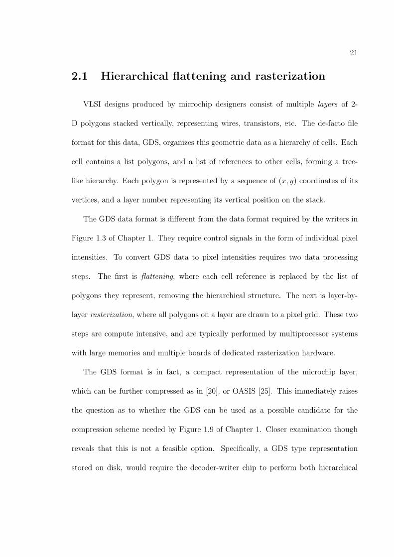
layer image. Image blocks 2048-pixel wide and 2048-pixel tall are sampled across each

microchip layer. Each image represents a 0.61 mm by 0.61 mm section of the chip,

covering about 0.1% of the chip area.

3 image samples are generated across each each layer, chosen by hand to cover

different areas of the chip design, Memory, Control, and a mixture of both Mixed.

The reason for hand sampling rather than random sampling has to do with limited

memory available to the hardware decoders as described in Chapter 1. Specifically,

because of limited memory, the compression ratio must be above a certain level across

all portions of the layer as much as possible. Consequently, by hand sampling, we

target areas of the design with a high density of geometric shapes which are difficult to

compress, in contrast to blank areas of the chip design, which are trivial to compress.

Similarly, the 3 layers sampled are the polysilicon layer (Poly) used to form tran-

sistor gates, and the primary and secondary wiring layers, Metal 1 and Metal 2 used

for wiring connections. In particular, Poly and Metal 1 are “critical layers”, and much

of the effort of designing a chip goes into these layers. The layout for these layers

resemble dense maze like structures of thin lines and spaces. Consequently, they have

high density of geometric shapes per unit area, and are difficult to compress. Metal

2 is a higher level metal layer with thicker wires and larger spaces, and therefore, it

is considerably less dense.

The compression results for these binary image samples are show in Table 2.1. The

first column is the name of the horizontal sample across a layer. “Memory” layout

37

Table 2.1: Compression ratios for JBIG, ZIP, and BZIP2 on 300 nm, binary layerimages.

Type Layer JBIG ZIP BZIP2

MemoryMetal 2 58.7 88.0 171Metal 1 9.77 47.9 55.5Poly 12.4 50.7 82.5

ControlMetal 2 47.0 22.1 24.4Metal 1 20.0 10.9 11.2Poly 41.6 18.9 23.2

MixedMetal 2 51.3 28.3 39.4Metal 1 21.2 11.9 12.1Poly 41.3 22.9 27.8

consists of densely arrayed, regularly repeating cells. “Control” layout is irregular

and less dense compared to memory. “Mixed” layout comes from a section of a chip

that contains some control intermingled with the memory cells. The second column

is the chip layer from which the sample is drawn. Compression ratios of JBIG, ZIP,

and BZIP2 are on columns 3 to 5, respectively. Each row represents compression

ratios for each of the sample binary layer images. As explained in Section 1.2, the

approximate compression ratio target, in order to achieve a throughput of one wafer

layer per minute, is 10. Ratios less than this threshold are highlighted in boldface.

Examining the column 3 of Table 2.1 reveals that JBIG performs better on con-

trol, mixed type layouts than on memory. It also performs better on metal 2 than

on metal 1 and poly. These layer images are sparser in terms of polygon density.

In particular, JBIG’s performance is lowest when applied to the most dense regular

layout, Metal 1 Memory. Even though the memory cells are very repetitive, JBIG’s

limited ten-pixel context is not enough to model this repetition of cells. Conceptu-

38

ally, we could increase the context size of the JBIG algorithm until it covers an entire

repetition cell. However, the complexity of JBIG’s context-based prediction mecha-

nism increases exponentially with the number of context pixels; so it is infeasible to

use more than a few tens of pixels, whereas cells easily span hundreds of pixels. The

effectiveness of JBIG-style prediction is explored more thoroughly in Chapter 4, when

we describe a compression algorithm custom tailored to layer image data. For now,

the key observation is that JBIG’s compression efficiency is inversely proportional to

geometric density.

In contrast to JBIG, ZIP’s compression ratios, shown in column 4, suggest that

it is well suited to compressing memory layout, exhibiting compression ratios of 50

or higher. The repetition of memory cells allows the ZIP algorithm to find plenty

of long matches, which translates into high compression ratios. On the other hand,

ZIP performs poorly on irregular layouts found in control and mixed layouts. For

these, ZIP is unable to find long matches, and frequently outputs literals, resulting

in performance loss in these areas. We examine the effectiveness of ZIP-style copying

more thoroughly in Chapter 3, which extends the effectiveness of ZIP (LZ77) copying

to two dimensional copy regions for image data.

In general the compression ratio of BZIP2 follows a pattern similar to ZIP across

the layer image samples, but with larger compression ratios. Block-sorting takes

advantage of the same repetition structure that ZIP does, but more efficiently, in part

because it operates on a significantly larger block of data, from 100KB to 900KB. This

39

is in contrast to the 4KB of memory which ZIP uses. The tradeoff between decoder

memory and compression efficiency is explored more thoroughly when we examine

implementation issues associated with the architecture presented in Figure 1.9.

Examining Table 2.1 row-by-row, it is evident that for each layer image sample, at

least one algorithm achieves the compression ratio target of 10. However, these com-

pression results are reported for an image with binary pixels, whereas the compression

ratio requirement of 10 is determined for an image with gray pixels. Certainly, if a

particular layer with 50 nm minimum feature size could be rasterized using 25 nm

pixels with black-and-white pixels, so that all edges are aligned on a 25 nm grid, for

that layer, the required output data rate can be reduced by a factor of 5. This can

potentially reduce the compression ratio requirement to 5, which is easily achieved by

all the techniques tested in Table 2.1. All four compression techniques remain strong

candidates for application to maskless lithography. To better extrapolate compres-

sion ratio achievable on future lithography data, we next consider the compression

results of more modern layer data.

2.6 Compression results of existing techniques for

layer image data with gray pixels

More recently, we have obtained the use of a GDS file containing the active layer

data of a piece of modern industry microchip with the understanding that this layer

40

Table 2.2: Compression ratios for SPIHT, JPEG-LS, RECT, ZIP, BZIP2, on 75 nm,5 bpp data

Image SPIHT JPEG-LS RECT ZIP BZIP2 BZIP2(100K) (900K)

active a 8.44 9.27 33.9 45.7 227 227active b 9.69 9.76 61.1 61.1 497 800active c 5.00 5.31 18.7 46.4 296 518active d 7.44 8.45 24.5 60.1 319 409active e 9.37 11.3 72.8 47.3 189 195

would be fabricated using state-of-the-art lithography tools capable of printing 150

nm feature sizes, with an edge placement accurate to approximately 5 nm. Applying

the rasterization methodology presented in Section 2.2, 150 nm feature size, using

2 pixels per minimum feature, equates to a 75 nm pixels. To achieve 5 nm edge

placement accuracy using 75 nm pixels requires 75/5 = 15 gray levels which rounds

up to 5 bits-per-pixel (bpp). Finally, polygons on the layer are placed on a 75 nm pixel

grid. Fully covered pixels are white, fully uncovered pixels are black, and partially

covered pixels are assigned a gray value equivalent to the fraction of area covered,

quantized to the nearest n/15. To this data we apply SPIHT image compression,

JPEG-LS image compression, a lossless version of the industry standard JPEG, ZIP

byte stream compression, another industry standard, BZIP2 byte stream compression,

and the RECT compressed representation. The results are presented in Table 2.2.

Column 1 of Table 2.2 names the layer image to which the compression techniques

are applied. Active a is a 1000× 1000 pixel image, corresponding to a 75µm× 75µm

square randomly selected from the center area of the chip. Active b is a 2000× 2000

pixel image, corresponding to a 150µm× 150µm square selected from the same area

41

as active a, and includes active a. Active c through active e are 2000 × 2000 pixel

images, corresponding to a 150µm× 150µm squares randomly selected from different

parts of the chip, covering approximately 0.01% of a chip. Each sample is visually

inspected to ensure that it is not mostly black.

The numbers in columns 2-7 are compression ratios for SPIHT, JPEG-LS, RECT,

ZIP, and BZIP2 respectively, with each row corresponding to one of the active layer

images. Comparing the second and third columns, JPEG-LS achieves slightly better

compression than SPIHT; however, ZIP, 2D-LZ, and BZIP2 outperform them by more

than a factor of 4. Even though SPIHT and JPEG-LS are state-of-the-art lossless

natural image compressors, they cannot take full advantage of the highly structured

nature of images generated from microchip designs. The fourth column RECT, rep-

resents the effective compression ratio achieved if no rasterization is performed, and

the relevant rectangles are stored in a list. A rectangle is considered relevant if any

portion of it intersects the area being rasterized. The size of the RECT representa-

tion increases linearly with the number of rectangles inside the rasterization region,

so a large “compression ratio” indicates few rectangles in the region, and a small

“compression ratio” indicates more rectangles in the region. RECT’s “compression

ratio” can therefore be interpreted as an inverse measure of rectangle density, which

varies dramatically in different areas of the layer. Although at times RECT performs

similarly to ZIP for active b and active e, it achieves less than half the compression

ratio of ZIP for active c and active d.

42

In the last four columns, compression ratios for ZIP, and BZIP2 are listed. For

BZIP2 there are two results corresponding to two different block sizes used for block

sorting, 100KB blocks and 900KB blocks. Impressively, all three techniques exceed

the target compression ratio of 10 with considerable margins. This is likely a function

of applying compression to the active layer, which is considerably less challenging

than Poly, Metal 1, and Metal 2 described previously, due to low polygon density. In

general, the compression ratio of BZIP2 exceeds that of ZIP. In the next chapter, we

will revisit the compression ratio of ZIP and BZIP2 applied to the more challenging

Poly, Metal 1, and Metal 2 layers of modern industry microchip design, in addition

to introducing two novel compression algorithms designed specifically for layer image

data.

43

Chapter 3

Overview of 2D-LZ Compression

In the preceding chapter, we have shown that LZ77 compression, as implemented

by ZIP, is quite effective at compression of layout data, surpassing state-of-the-art

image compression algorithms such as SPIHT and JPEG-LS. On the other hand, LZ77

is an inherently one-dimensional algorithm, which suggests that there may be room

for improvement, because layer image data is certainly 2 dimensional. In response to

this basic observation, we developed 2D-LZ, a two-dimensional variant of the LZ77

algorithm [3] [4]. In the remainder of this chapter, we provide an brief overview of

2D-LZ and characterize its performance. In doing so, we show that while 2D-LZ is

well suited to compressing repetitive layouts, it is ineffective for irregular layouts.

44

(x,y)

height

width

Match region

Not yet coded

Previously coded

Search region

Figure 3.1: 2D-LZ Matching

3.1 A Brief Introduction to the 2D Matching Al-

gorithm

The 2D-LZ algorithm extends the LZ77 algorithm to two dimensions, thereby tak-

ing advantage of the inherent two-dimensional nature of layout data, for the system

architecture proposed in Chapter 1. Pixels are still encoded using raster scan order.

However, the linear search window, which appears in LZ77, is replaced with a rect-

angular search region of previously coded pixels. This search window is illustrated in

Figure 3.1.

As illustrated in Figure 3.1, a match is now a rectangular region, specified with four

coordinates: a pair of coordinates, (x, y), specify the match position, and another pair

of integers, (width, height), specify the extent of the match. If a match of minimum

size cannot be found, then a literal is outputted representing a vertical column of

pixels. A sequence of control bits is also stored so the decoder can determine whether

the output is a literal or a match. To further compress the output, five Huffman

45

codes are used: one for each of the match coordinates x, y, width, height, and one for

the literal.

2D-LZ behaves similarly to LZ77 in that longer matches and frequent repetitions

increase the compression ratio. Therefore, several complex heuristics are employed in

2D-LZ to maximize the size of match regions, with the goal of improving compression

efficiency for repetitive layouts. A more detailed explanation of these heuristics can

be found in [3].

The decoding of 2D-LZ is simple. First the match region x, y, width, and height,

and the literals are Huffman decoded. Similar to the encoder, the decoder also keeps

a buffer of previously decoded pixels. The size of this buffer must be large enough

to contain the height of the search window and the width of the image for matching

purposes. Each time a match is read, the decoder simply copies data from the cor-

responding match region among the previously decoded pixels and fills it in the not

yet decoded area. If a literal is read, the decoder simply fills in a vertical column of

pixels in the not yet coded area. The decoder does not need to perform any searches,

and is therefore much simpler in design and implementation than the encoder.

3.2 2D-LZ compression results

In Table 3.1, we compare 2D-LZ compression against JBIG, ZIP, and BZIP2 on the

same binary image layouts as presented in Chapter 2. These binary images contained

various layers of several layout types such as memory, control, and mixed logic. The

46

Table 3.1: Compression ratio for 2D-LZ, as compared to JBIG, ZIP, and BZIP2 on300 nm, binary layer images.

Type Layer JBIG ZIP BZIP2 2D-LZ

MemoryMetal 2 58.7 88.0 171 233Metal 1 9.77 47.9 55.5 79.1Poly 12.4 50.7 82.5 120

ControlMetal 2 47.0 22.1 24.4 25.5Metal 1 20.0 10.9 11.2 11.2Poly 41.6 18.9 23.2 20.4

MixedMetal 2 51.3 28.3 39.4 34.4Metal 1 21.2 11.9 12.1 12.6Poly 41.3 22.9 27.8 27.2

Decoder Buffer (kB) - 4 128 32

Table 3.2: Compression ratio for 2D-LZ, as compared to SPIHT, JPEG-LS, RECT,ZIP, BZIP2, on 75 nm, 5 bpp data

Image SPIHT JPEG-LS RECT ZIP BZIP2 BZIP2 2D-LZ(100) (900)

active a 8.44 9.27 33.9 45.7 227 227 111active b 9.69 9.76 61.1 61.1 497 800 144active c 5.00 5.31 18.7 46.4 296 518 328active d 7.44 8.45 24.5 60.1 319 409 273active e 9.37 11.3 72.8 47.3 189 195 145

Decoder Buffer (kB) - - - 4 100 900 262

compression ratio of 2D-LZ is shown in column 6. In general, 2D-LZ performs about

the same as BZIP2, and better than ZIP. For memory cells in particular, 2D-LZ

compresses twice as well as ZIP. Memory cells are regularly arrayed both vertically

and horizontally, and 2D-LZ takes full advantage of this two-dimensional repetition.

For irregular layout found in control and mixed logic, 2D-LZ exhibits a performance

loss as compared to JBIG.

In Table 3.2, we compare 2D-LZ compression against SPIHT, JPEG-LS, RECT,

ZIP, 2D-LZ, and BZIP2 on the same gray pixel image layouts as presented in Chapter

47

2. These gray pixel images are taken from the active layer of an industry layout. The

compression ration of 2D-LZ is shown in column 8. Again 2D-LZ performs slightly

worse than BZIP2, significantly better than ZIP, and RECT, and far exceeds the

efficiency of JPEG-LS and SPIHT.

In summary, even though 2D-LZ exceeds the performance of ZIP by taking advan-

tage of the 2D structure of layout data, it remains highly optimized for compressing

repetitive layout. Specifically, it still retains the basic weakness of the LZ77 algorithm

in that for irregular layout where large repetitive regions cannot be found, 2D-LZ still

cannot exceed the compression efficiency of the JBIG algorithm. This observation is

the genesis for the C4 algorithm, as we search for a way to combine the best aspects

of 2D-LZ and JBIG, without the large buffering requirements of BZIP2.

48

Chapter 4

Context-Copy-Combinatorial

Coding (C4)

Our work with existing algorithms as well as 2D-LZ shows that layout data has

2 major qualities to be exploited for lossless compression. First it is highly repeti-

tive, and this is the used by LZ77 and 2D-LZ to achieve high compression efficiency.

Second, where the layout is not repetitive, it can be compressed by context-based

prediction schemes such as JBIG. In developing C4, we attempt to fuse these 2 ideas

into a single compression algorithm, applicable to repetitive and non-repetitive lay-

outs alike.

49

4.1 C4 Compression

The basic concept underlying C4 compression is to integrate the advantages of

two disparate compression techniques: local context-based prediction and LZ-style

copying, as characterized by JBIG and 2D-LZ respectively. This is accomplished

through automatic segmentation of an image into copy regions and prediction regions.

Each pixel inside a copy region is copied from a pixel preceding it in raster-scan

order. Each pixel inside a prediction region, i.e. not contained in any copy region, is

predicted from its local context. However, neither predicted values nor copied values

are 100% correct, so error bits are used to indicate the position of these prediction or

copy errors. These error bits can be compressed using any binary entropy coder, but

in C4, we apply a new technique called hierarchical combinatorial coding (HCC) to

be described shortly as a low-complexity alternative to arithmetic coding. Only the

copy regions and compressed error bits are transmitted to the decoder.

In addition, as discussed in Chapter 1, for our application to direct-write maskless

lithography, the C4 decoding algorithm must be implemented in hardware as a parallel

array of thousands of C4 decoders fabricated on the same substrate as a massively

parallel array of writers [4]. As such, the C4 decoder must have a low implementation

complexity. In contrast, the C4 encoder is under no such complexity constraint.

This basic asymmetry in the complexity requirement between encoding and decoding,

which is common to many compression applications, is central to the design of the

C4 algorithm.

50

Fig. 4.1 shows a high-level block diagram of the C4 encoder and decoder for binary

layer images. First, a prediction error image is generated from the layer image, using

a simple 3-pixel context-based prediction model. In generating this prediction error

image, we assume as a starting point that the entire image is encoded using context

based prediction. Next, we successively add copy regions onto the background pre-

diction region where appropriate, in order to further improve compression efficiency.

The reason that prediction is used as “background” is that it is globally applicable

to layout as a whole, whereas copy regions are specific to repetitive layout, and the

period of repetition varies from region to region. The result is a segmentation map

of copy regions on top of a prediction region background.

As specified by the segmentation map, the Predict/Copy block estimates each

pixel value, either by copying or by prediction. The result is compared to the actual

value in the layer image. Correctly predicted or copied pixels are indicated with a

“0”, and incorrectly predicted or copied pixels are indicated with a “1”, equivalent

to a Boolean XOR of predicted/copied pixel values with the original layer image.

These error bits are compressed without loss by the Hierarchical Combinatorial Code

(HCC) encoder, which are transmitted to the decoder, along with the segmentation

map. The segmentation map itself is represented as a list of copy region rectangles,

with each rectangle specified by its position (x, y), size (w, h), and copy parameters

(left/above, d) in binary format.

The decoder mirrors the encoder, but skips the complex steps necessary to find

51

Compute prediction

error image

Find copy

regions Layout

error bits

segmentation

error bits

Predict/Copy

Compare XOR

HCC Decoder

Predict/Copy

Layout Correction XOR

HCC Encoder

Decoder

Encoder

segmentation

segmentation

Figure 4.1: Block diagram of C4 encoder and decoder for binary images.

the segmentation map, which are received from the encoder. Again as specified by the

segmentation, the Predict/Copy block estimates each pixel value, either by copying

or by prediction. The HCC decoder decompresses the error bits from the encoder. If

the error bit is “0” the prediction or copy is correct, and if the error bit is “1” the

prediction or copy is incorrect and must be inverted, equivalent to a per-pixel Boolean

XOR operation between the error bit and the estimated pixel value. Since there is no

data modeling performed in the C4 decoder, it is considerably simpler to implement

than the encoder, satisfying one of the requirements of our application domain.

52

Table 4.1: The 3-pixel contexts, prediction, and the empirical prediction error prob-ability for a sample layer image

Context Prediction Error Error probability

0.0055

0.071

0.039

0

0

0.022

0.037

0.0031

4.2 Context-based Prediction Model

For our application domain, i.e. microchip layer image compression, we use a

simple 3-pixel binary context-based prediction model in C4, which is much simpler

that the 10-pixel model used in JBIG [8]. Since the number of contexts scales ex-

ponentially with the number pixels used for prediction, this represents a significant

complexity reduction of the C4 prediction mechanism at the decoder, as compared to

JBIG. Nonetheless, this simple 3-pixel context captures the essential “Manhattan”

structure of layer data, as well as some design rules, as seen in Table 4.1.

The pixels used to predict the current coded pixel are the ones above, left, and

above-left of the current pixel. The first column shows the 8 possible 3-pixel contexts,

the second column shows the prediction, the third column shows what a prediction

error represents, and the fourth column shows the empirical prediction error proba-

53

(a) (b)

Figure 4.2: (a) Non-repetitive layer image data and (b) its resulting prediction errorimage.

bility for an example layer image. From these results, it is clear that the prediction

mechanism works extremely well. Layer data is dominated by vertical edges, hori-

zontal edges, and regions of constant intensity. The simple 3-pixel context predicts

all these cases perfectly. Consequently, we do not expect much benefit to increasing

the number of context pixels to 4 or higher, and in fact, this intuition matches our

empirical observations. Visual inspection of the prediction error reveals that predic-

tion errors primarily occur at the corners in the layer image. The two exceptional 0%

error cases in rows 5 and 6 represent design rule violations.

To generate the prediction error image, each correctly predicted pixel is marked

with a “0”, and each incorrectly predicted pixel is marked with a “1”, creating a

binary image which can be compressed with a standard binary entropy coder. The

fewer the number of incorrect predictions, the higher the compression ratio achieved.

54

(a) (b)

Figure 4.3: (a) Dense repetitive layer image data and (b) its resulting prediction errorimage.

In fact, as we shall explain shortly, this “prediction only” mode is used as a basis

of comparison for generating copy regions, i.e. a copy region is added only if it

improves the overall compression efficiency as compared to simply using context-

based prediction everywhere.

Alternatively, it is also possible to group pixels by their context, forming 8 sep-

arate binary streams, each to be compressed separately by its own entropy coder.

Empirically, for layer images, we have found that operating on the prediction error

image is nearly as efficient as grouping pixels by context.

An example of non-repetitive layout for which prediction works well is shown in

Fig. 4.2(a), and its corresponding prediction error image is shown in Fig. 4.2(b).

In contrast to the non-repetitive layout shown in Fig. 4.2(a), some layer image

55

data contains regions that are visually “dense” and repetitive. An example of such

a region is shown in Fig. 4.3(a). This visual “denseness” results in a dense, large

number of prediction errors as seen clearly in the prediction error image in Fig. 4.3(b).

The high density of prediction errors translates into low compression ratios using

prediction alone. In C4, areas of dense repetitive layout are covered by copy regions

to reduce the number of errors, as described in Section 4.3.

4.3 Copy Regions and Segmentation

As seen in Fig. 4.3(a) of the previous section, some layer images are highly repeti-

tive. We can take advantage of this repetitiveness to achieve compression by specifying

copy regions, i.e. a rectangular region that is copied from another rectangular region

preceding it in raster-scan order.

The copy itself can be defined both in the layer image data domain, or the pre-

diction error image domain. Although there is a one-to-one correspondence between

the two images, copy regions defined in one domain are not the same as the other

domain. Nonetheless, they are extremely similar, differing only at the boundaries of

the copy regions. Tests on layout show negligible differences in compression efficiency

between these two approaches. C4 defines copy regions on the layer image data, which

is perhaps the more intuitive of the two choices.

A copy region in C4 is defined as a rectangle inside which every pixel is copied

from either d pixels to its left, or d pixels above. Consequently the region is com-

56

w

h

d (x,y)

Figure 4.4: Illustration of a copy left region.

pletely specified by six parameters: (x, y) position of the upper left hand corner of

the rectangle, the size of the rectangle (w, h), the copy direction (dir = left/above)

and the copy distance d. An example of a copy region is illustrated in Figure 4.4.

In the figure, the dashed red rectangle is the copy region. It is positioned at (x, y),

has size (w, h), and every pixel inside it is copied d pixels from the left as indicated

by the arrow. Although the entire region is copied, the copy itself need not be 100%

correct. Similar to the prediction error map, there is a corresponding copy error map

within the copy region. Each correctly copied pixel is indicated with a “0”, and each

incorrectly copied pixel each incorrectly predicted pixel is marked with a “1”, creating

a binary sub-image which can be compressed with a standard binary entropy coder.

This method of copying is related to LZ77 [6] copying, but extended to two di-

mensions (2D) with errors allowed. Conceptually, this allows us to capture the 2D-

repetitions found in layer images. In addition, note that in Fig. 4.4 the single copy

region spans three horizontal periodic repetitions, with period d. In C4, an entire

57

periodic array can be described with a single copy region. This simple feature is

extremely important for extracting compression efficiency from layer data, which can

contain large periodic 2D-arrays.

This method of copying contrasts sharply with the method of copying used in

JBIG2 [9] called “soft-pattern matching” [17], which constructs an explicit dictionary

of pixel blocks that can be throughout the image. In JBIG2, each individual copy in

a 2D periodic array must be separately referenced [9], leading to a lower compression

efficiency in comparison to C4 for this type of data.

The C4 copy mechanism is a restricted version of the copy mechanism allowed by

2D-LZ in Figure 3.1. Whereas 2D-LZ allows copies from any direction, C4 restricts

the copy direction to (dir = left/above). This restriction allows C4 to significantly

expand the copy distance d beyond that allowed by 2D-LZ while reducing the number

of bits needed to represent copies. For example, to specify copy from any direction

in a 256 pixel square region is equivalent to specifying a point (cx, cy) in that region

which takes 8 bits for cx and 8 bits for cy. So 2D-LZ uses 16-bits to specify a copy

direction and distance within a 256 pixel square region. In contrast C4 uses one bit

to specify the copy direction (dir = left/above) and allows the copy distance d to

extend to 1024-pixels which takes 10-bits to represent. So C4 uses 11-bits to represent

a copy direction and distance, 5 fewer bits than 2D-LZ. This tradeoff means that C4

can better compress horizontal and vertical repetitions with fewer bits in comparison

to 2D-LZ, at a cost of disallowing diagonal copies. This tradeoff is worthwhile because

58

of the Manhattan structure of layout design.

As described in Section 4.1, the C4 encoder automatically segments the image

into copy regions and the prediction region, i.e. all pixels not contained in any

copy region. Each copy region has its own copy parameters and corresponding copy

error map, and the background prediction region has a corresponding prediction error

map. Together, the error maps merge to form a combined binary prediction/copy

error map of the entire image, which is compressed using HCC as a binary entropy

coder. The lower the number of the total sum of prediction and copy errors, the

higher the compression ratio achieved. However, this improvement in compression

by the introduction of copy regions, is offset by the cost in bits to specify the copy

parameters (x, y, w, h, left/above, d) of each copy region. Moreover, copy regions that

overlap with each other are undesirable: each pixel should ideally only be coded once,

to save as many bits as possible.

Ideally, we would like the C4 encoder to find the set of non-overlapping copy

regions, which minimizes the sum of number of compressed prediction/copy error bits,

plus the number of bits necessary to specify the parameters of each copy region. An

exhaustive search over this space would involve going over all possible non-overlapping

copy region sets i.e. a combinatorial problem, generating the error bits for each set,

and performing HCC compression on the error bits. This is clearly infeasible. To

make the problem tractable, a number of simplifying assumptions and approximate

metrics are adopted.

59

First we use entropy as a heuristic to estimate the number of bits generated by the

HCC encoder to represent error pixels. If p denotes the percentage of prediction/copy

error pixels over the entire image, then error pixels are assigned a per-pixel cost of

C = −log2(p) bits, and correctly predicted or copied pixels are assigned a per-pixel

cost of −log2(1 − p) ≈ 0. Of course, given a segmentation map, p can be easily

measured by counting the number of prediction/copy error bits; at the same time,

p affects how copy regions are generated in the first place, as discussed shortly. In

C4, we solve this chicken and egg problem by first estimating a value of p, finding a

segmentation map using this value, counting the percentage of prediction/copy error

pixels, and using this percentage as a new value for p as input to the segmentation

algorithm. This process can be iterated until the estimated p matches the percentage

of error pixels; however, in practice we find that one iteration is sufficient if the

starting estimate is reasonable. Empirically, we have found a reasonable starting

estimate to be the percentage of error pixels when no copy regions are used, then

discounted by a constant factor of 4.

Next, for any given copy region, we compare the cost, in bits, of coding that region

using copy, versus the cost of coding the region using prediction. If the cost of copying

is lower, then the amount by which it is lower is the benefit of using this region. The

cost of copying is defined as the sum of the cost of describing the copy parameters,

plus the cost of coding the copy error map. For our particular application domain,

the description cost is 51 bits. Here we have restricted x, y, w, h to 10-bits each

60

which is reasonable for our 1024 × 1024 test images. In addition, the copy direction

and distance (left/above, d) can be represented with 11 bits, where d, represented by

10 bits, denotes the distance left or above to copy from, and left/above, represented

by 1 bit, denotes the direction left or above to copy from. The cost of coding the copy

error map is estimated as C ×Ecopy, where C denotes the estimated per-pixel cost of

an error pixel, as discussed previously, and Ecopy denotes the number of copy error

pixels in the region. Correctly copied pixels are assumed to have 0 cost, as discussed

previously. So the total cost of copying is 51 + C × Ecopy.

The cost of coding the region using prediction is the cost of coding the prediction

error map of that region. It is estimated as C × Econtext , where Econtext denotes

the number of prediction error pixels in the region. Finally, the benefit of a region

is the difference between these two costs, C × (Econtext − Ecopy) − 51 . Note that

it is possible for a region to have negative benefit if Econtext − Ecopy ≤ (51/C). The

threshold T = (51/C) is used to quickly disqualify potential copy regions in the search

algorithm presented below.

Using benefit as a metric, the optimization goal is to find the set non-overlapping

copy regions, which maximizes the sum of benefit over all regions. This search space

is combinatorial in size, so exhaustive search is prohibitively complex. Instead we

adopt a greedy approach, similar to that used in the 2D-LZ algorithm described in

[4]. The basic strategy used by the find copy regions algorithm in Fig. 4.1 is as

follows: start with an empty list of copy regions; and in raster-scan order, add copy

61

regions of maximum benefit, that do not overlap with regions previously added to

the list. The completed list of copy regions is the segmentation of the layer image.

A detailed flow diagram of the find copy regions algorithm is shown in Fig. 4.5, and

described in the remainder of this section.

In raster-scan order, we iterate through all possible (x, y). If (x, y) is inside any

region in the segmentation list, we move on to the next (x, y); otherwise, we iterate

through all possible (left/above, d). Next for a given (x, y, left/above, d), we max-

imize the size of the copy region (w, h) with the constraint that a stop pixel is not

encountered; we define a stop pixel to be any pixel inside a region in the segmentation

list, or any pixel with a copy error. These conditions prevent overlap of copy regions,

and prevent the occurrence of copy errors, respectively. Later, we describe how to

relax this latter condition to allow for copy errors. The process of finding maximum

size copy regions (w, h), is discussed in the next paragraph. Finally, we compute the

benefit of all the maximum sized copy regions, and, if any region with positive benefit

exists, we add the one with the highest positive benefit to the segmentation list.

We now describe the process of finding the maximum size copy region (w, h). For

any given (x, y, left/above, d) there is actually a set of maximum size copy regions,

bordered by stop pixels, because (w, h) is a two-dimensional quantity. This is il-

lustrated in the example in Fig. 4.6. In the figure, the position of the stop pixels

are marked with ⊗ and three overlapping maximum copy regions are shown namely

(x, y, w1, h1) (x, y, w2, h2) and (x, y, w3, h3). The values w1, h1, w2, h2, w3, and h3 are

62

Begin find copy regions

Generate next (x,y) in raster order

Is (x,y) inside

segmentation region?

Generate next (left/above, d)j

Find maximum size copy regions

{(w1,h1), (w2,h2),…,(wi,hi),…}

Initialize segmentation to empty list

Evaluate benefiti for each (wi,hi)

Find region of highest benefit over all i

(x,y,(left/above,d,(w,h,benefit)maxi)j)

Is last (left/above,d)j?

Find region of highest benefit over all j

(x,y,(left/above,d,(w,h,benefit)maxi)maxj)

If benefitmaxi,maxj > 0

add region to the segmentation list

Is last (x,y)?

Output segmentation list

End find copy regions

yes

no

yes

yes

no

no

Figure 4.5: Flow diagram of the find copy regions algorithm.

63

(x,y)

(w1,h1)(w2,h2)

(w3,h3)

w1

h1

Figure 4.6: Illustration of three maximum copy regions bordered by four stop pixels.

found using the following procedure: initialize w = 1, h = 1. Increment w until a

stop pixel is encountered; at this point w = w1. Next increment h, and for each h,

increment w from 1 to w1, until a stop pixel is encountered; at this point h = h1, and

w = w2. Again increment h, and for each h increment w from 1 to w2, until a stop

pixel is encountered; at this point h = h2, and w = w3. Finally, increment h, and

for each h increment w from 1 to w3, until a stop pixel is encountered; at this point

h = h3, and w = 1. The maximum size algorithm is terminated when a stop pixel is

encountered at w = 1.

As stated previously, any pixel inside a region in the segmentation list, and any

pixel with a copy error, is a stop pixel. Recall in the algorithm to find maximum size

copy regions, the stop-pixel limits the copy region from expanding further. We relax

the definition of a stop-pixel to merge smaller, error free, copy regions, into larger

copy regions with a few number of copy errors. The basic premise is to tradeoff the

51-bits necessary to describe a new copy region against the introduction of bits needed

to code copy errors, by excluding some copy error pixels from being stop pixels. For

each copy error pixel, we examine a look-ahead window (LAW) of W pixels in a row,

64

where the left most pixel is the copy error. For this LAW we consider 3 scenarios.

First suppose the current copy region is extended to include the LAW. In the

LAW, there is at least one copy error of course, but possibly a few more. Let us

denote this quantity as Ecopy.

Next suppose the current copy region is not extended to include the LAW. Then

the LAW could be entirely part of a background prediction region. Assuming the

LAW is entirely a prediction region, we can count the number prediction errors and

denote it as Epredict.

Finally, suppose in the final segmentation neither the current copy region, nor the

background region covers the entire LAW. It could be that the LAW is covered by an

unknown mix of copy regions and prediction regions. In this case, our target is to do

no worse than the expected number of errors in a LAW of W pixels = Wp

Suppose in the final result Ecopy < Epredict, this indicates that for the LAW, it is

better to continue the copy region than it is to allow this area to become a predict

region.

Suppose in the final result Ecopy < Wp, this indicates that for the LAW, continuing

the copy region would do better than our expectation.

If both of these are true, then reasoning would indicate that it is likely to be

advantageous to extend the copy region than to cut it off. In this case, that specific

copy error at the left-most pixel of the LAW is no longer treated as a stop-pixel for

the purpose of maximizing the copy region.

65

The size of the look-ahead window W is a user-defined input parameter to the C4

algorithm. Empirically, larger values of W correspond to fewer, larger copy regions,

at the expense of increasing the number of copy errors. Note that if W is sufficiently

small, such that Wp < 1, then copy errors are effectively disallowed, as Ecopy > 1.

4.4 Hierarchical Combinatorial Coding (HCC)

We have proposed and developed combinatorial coding (CC) [10] as an alternative

to arithmetic coding to encode the error bits in Fig. 4.1. The basis for CC is universal

enumerative coding [11] which works as follows. For any binary sequence of known

length N , let k denote the number of ones in that sequence. k ranges from 0 to N ,

and can be encoded using a minimal binary code [14], i.e. a simple Huffman code

for uniform distributions, using dlog2(N + 1)e bits. There are exactly C(N, k) =

N !/(N −k)!k! sequences of length N with k ones, which can be hypothetically listed.

The index of our sequence in this list, known as the ordinal or rank, is an integer

ranging from 1 to C(N, k), which can again be encoded using a minimal binary code,

using dlog2C(N, k)ebits. Enumerative coding is theoretically shown to be optimal [11]

if the bits to be compressed are independently and identically distributed (i.i.d.) as

Bernoulli(θ) where θ denotes the unknown probability that “1” occurs, which in C4,

corresponds to the percentage of error pixels in the prediction/copy error map. The

drawback of computing an enumerative code directly is its complexity: the algorithm

to find the rank corresponding to a particular binary sequence of length N , called

66

ranking in the literature, is O(N) in time, is O(N) in memory, and requires O(N) bit

precision arithmetic [11].

In CC, we address this problem by first dividing the bit sequence into blocks of

fixed size M . For today’s 32-bit architecture computers, M = 32 is a convenient

and efficient choice. Enumerative coding is then applied separately to each block,

generating a (k, rank) pair for each block. Again, using the same assumption that

input bits are i.i.d. as Bernoulli(θ), the number of ones k in a block of M bits are

i.i.d. as Binomial(M, θ). Even though the parameter θ is unknown, as long as the

Binomial distribution is not too skewed, e.g. 0.01 < θ < 0.99, a dynamic Huffman

code efficiently compresses the k-values with little overhead, because the range of k

is small. Given there are k ones in a block of M bits, the rank remains uniformly

distributed, as in enumerative coding. Therefore, rank-values are efficiently coded

using a minimum binary code.

The efficiency of CC, as described, is on par with arithmetic coding, except in

cases of extremely skewed distributions, e.g. θ < 0.01. In these cases, the probability

that k = 0 approaches 1 for each block, causing the Huffman code to be inefficient.

To address this issue, we have developed an extension to CC called hierarchical com-

binatorial coding (HCC). It works by binarizing sequence of k-values such that k = 0

is indicated with a “0” and k = 1 to 32 is indicated with a “1”. CC is then applied to

the binarized sequence of “0” and “1”, and the value of k, ranging from 1 to 32 in the

“1” case, is Huffman coded. Clearly, this procedure of CC encoding, binarizing the

67

k-values, then CC encoding again can be recursively applied in a hierarchical fashion,

to take care of any inefficiencies in the Huffman code for k-values, as θ approaches 0.

Figure 4.7 is an example of HCC in action with 2-levels of hierarchy and block

size M = 4. Only values in bold italics are coded and transmitted to the decoder.

Looking at rows from bottom to top, the original data is in the lowest row labeled

“bits – level 0”. Applying CC with M = 4, the next two rows show the rank and

k value for each block in level 0. Note that when k = 0 no rank value is needed as

indicated by the hyphen. The high frequency of 0 in “k – level 0” makes it inefficient

for coding directly using Huffman coding. Instead, we binarize “k – level 0”, to form

“bits – level 1”, using the binarization procedure described in the previous paragraph.

CC is recursively applied to “bits – level 1”, to compute “rank – level 1” and “k –

level 1”. Finally, to code the data, “k – level 1” is coded using a Huffman code, “rank

– level 1” is coded using a minimal binary code, non-zero values of “k – level 0” are

coded using a Huffman code, and “rank – level 0” is coded using a minimal binary

code.

The rationale for choosing Huffman coding and minimal binary coding is the same

as CC. If the input is assumed to be i.i.d. as Bernoulli(θ), then the distribution of

rank – level i given k – level i is uniformly distributed from 1 to C(M, k). Further-

more, although the exact distribution of k-values is unknown, a dynamic Huffman

code can adapt to the distribution with little overhead, because the dynamic range

of k – level i is small. Finally, for highly skewed distributions of k – level i, which

68

0000 0000 0000 0000 0010 0000 1010 0000

0 0 0 0 1 0 2 0

0000 1010

0 2

bits - level 0

k - level 0

bits - level 1

k - level 1

- 2 rank – level 1

- - - - 3 - 2 - rank – level 0

Figure 4.7: 2-level HCC with a block size M = 4 for each level.

hurts the compression efficiency of Huffman coding, the binarization process reduces

the skew by removing the most probable symbol k = 0.

Studying the example in Fig. 4.7, we can intuitively understand the efficiency

of HCC: the single Huffman coded 0 in “k – level 1” decodes to M2 zeroes in “bits

– level 0”. In general, for L-level HCC, a single Huffman coded 0 in level L − 1

corresponds to ML zeroes in “bits - level 0”. HCC’s ability to effectively compress

blocks of zeroes is critical to achieving high compression ratios, when the percentage

of the error pixels is low. In this HCC operates similiarly to various run-length codes,

which also focus on compacting blocks of 0’s. The differences are highlighted below.

In addition to achieving efficient compression, HCC also has several properties

favorable to our application domain. First, the decoder is extremely simple to im-

plement: the Huffman code tables are small because the range of k-values is small,

unranking is accomplished with a simple table lookup, comparator, and adder, and

69

minimal binary decoding is also accomplished by a simple table lookup and an adder.

Second, the decoder is fast: blocks of M (L+1) zeroes can be decoded instantly when

a zero is encountered at level L. Third, HCC is easily parallelizable: block sizes are

fixed and block boundaries are independent of the data, so the compressed bitstream

can be easily partitioned and distributed to multiple parallel HCC decoders. This is

in contrast to run-length coding schemes such as Golomb codes [12], which also code

for runs of zeroes, but have data-dependent block boundaries.

Independent of our development of HCC, a similar technique called Hierarchical

Enumerative Coding (HEC) has been developed in [13]. The main difference between

HEC and HCC is the method of coding k values at each level. HCC uses binarization

and simple Huffman coding, whereas HEC uses hierarchical integer enumerative cod-

ing, which is more complex [13]. Due to this complexity, at higher levels of hierarchy,

HEC merges 2 groups at a time, whereas HCC merges M groups, e.g. M = 32,

together through binarization. Consequently, HCC requires fewer levels of hierarchy

to achieve the same level of compression efficiency as HEC.

To compare HCC with existing entropy coding techniques, we apply 3-pixel con-

text based modeling as described in Section 4.2 to a 242 kb layer image, and group

pixels by context into 8 binary streams. We then apply Huffman coding to blocks of

8-bits, arithmetic coding, Golomb run-length coding, HEC, and HCC to each binary

stream, and report the compression ratio obtained by each algorithm. In addition,

we report the encoding and decoding times as a measure for complexity of these

70

Table 4.2: Result of 3-pixel context based binary image compression on a 242 kb layerimage for a P3 800 MHz processor

Metric Huf8 Arith. Golomb HEC HCCComp. ratio 7.1 47 49 48 49Enc. time(s) 0.99 7.46 0.52 2.43 0.54Dec. time(s) 0.75 10.19 0.60 2.11 0.56

algorithms. The results are shown in Table 4.2.

Among these techniques, HCC is one of the most efficient in terms of compression,

and one of the fastest to encode and decode, justifying its use in C4. The only algo-

rithm comparable in both efficiency and speed, among those tested, is Golomb run-

length coding. However, as previously mentioned, HCC has fixed, data-independent

block boundaries, which are advantageous for parallel hardware implementations;

run-length coding does not. Run-times are reported for 100 iterations on an 800 MHz

Pentium III workstation. All algorithms are written in C# and optimized with the

assistance of VTune to eliminate bottlenecks. The arithmetic coding algorithm is

based on that described in [14].

4.5 Extension to Gray Pixels

So far, C4 as described is a binary image compression technique. To extend C4

to encode 5-bit gray-pixel layer image, slight modifications need to be made to the

prediction mechanism, and the representation of the error. Specifically, the local 3-

pixel context based prediction described in Section 3, is replaced by 3-pixel linear

prediction with saturation, to be described later; furthermore, in places of prediction

71

compressed error value

error location error value

Compute prediction

error image

Find copy

regions Layout

segmentation Predict/Copy

Compare

HCC Decoder

Predict/Copy

Layout Buffer

Merge

HCC Encoder

Decoder

Encoder

Huffman Encoder

Huffman Decoder error location error value

compressed error location

Figure 4.8: Block diagram of C4 encoder and decoder for gray-pixel images.

or copy error, where the error location bit is ”1”, an error value indicates the correct

value of that pixel. A block diagram of the C4 encoder and decoder for gray-pixel

images is shown in Fig. 4.8.

First, a prediction error image is generated from the layer image, using a simple

3-pixel linear prediction model. The error image is a binary image, where “0” denotes

a correctly predicted gray-pixel value and “1” denotes a prediction error. The copy

regions are found as before in binary C4, with no change in the algorithm. As specified

by the copy regions, the Predict/Copy generates pixel values either using copying

or linear prediction. The result is compared to the actual value in the layer image.

Correctly predicted or copied pixels are indicated with a “0”, and incorrectly predicted

72

a b

c ?

x = b – a + c if (x < 0) then ? = 0

if (x > max) then ? = max

otherwise ? = x

Figure 4.9: 3-pixel linear prediction with saturation used in gray-pixel C4.

or copied pixels are indicated with a “1” with an error value generated indicating the

true value of the pixel. The error location bits are compressed with a HCC encoder,

and the actual error values are compressed with a Huffman encoder.

As in binary C4, the gray-pixel C4 decoder mirrors the encoder, but skips the

complex steps necessary to find the copy regions. The Predict/Copy block generates

pixel values either using copying or linear prediction according to the copy regions.

The HCC decoder decodes the error location bits, and the Huffman decoder decodes

the error values. If the error location bit is “0” the prediction or copy is correct, and

if the error location bit is “1” the prediction or copy is incorrect and the actual pixel

value is the error value.

The linear prediction mechanism used in gray-pixel C4 is analogous to the context-

based prediction used in binary C4. Each pixel is predicted from its 3-pixel neighbor-

hood as shown in Fig. 4.9. x is predicted as a linear combination of its local 3-pixel

neighborhood a, b, and c, using the equation x = b − a + c. Intuitively, there are

several ways to understand this formula. First, rewriting as x − c = b − a it says

the change moving right from a to b is the same as the change moving right from c

to x. Second, rewriting as x − b = c − a it says the change moving top to bottom

from a to c, is the same as the change moving top to bottom from b to x. Taken

73

Table 4.3: Compression ratios of JBIG, JBIG2, ZIP, 2D-LZ, BZIP2 and C4 for 2048×2048 binary layer image data.

Type Layer JBIG JBIG2 ZIP 2D-LZ BZIP2 C4Mem. M2 59 68 88 233 260 332Cells M1 10 12 48 79 56 90

Poly 12 14 51 120 83 141Ctrl. M2 47 52 22 26 32 50Logic M1 20 23 11 11 11 22

Poly 42 43 19 20 23 45

Encode Time (s) 6 11 2 640 4 720Decode Time (s) 6 7 1 2 4 2Decode Buffer (kB) - - 4 64 512 512

together, this means that the local derivative in both the x and y directions remains

constant, i.e. x is predicted to lie on the same 2D plane as a, b, and c. Specifically for

Mahattan layout, it means horizontal edges are predicted to continue, vertical edges

are predicted to continue, and regions of constant intensity remain constant. If the

prediction value x is negative or exceeds the maximum allowed pixel value max, the

result is clipped to 0 or max respectively. Interestingly, this linear predictor can also

be applied to a binary image by setting max = 1, resulting in the same predicted

values as binary context-based prediction described in Section 4.2. It is also similar

to the median predictor used in JPEG-LS [16].

4.6 Compression Results

We apply a suite of existing and general lossless compression techniques as well

as C4 to binary layer image data. Compression results are listed in Table 4.3. The

original data are 2048 × 2048 binary images with 300 nm pixels sampled from an

74

industry microprocessor microchip, which corresponds to a 0.61 mm by 0.61 mm

section, covering about 0.1% of the chip area. Each entry in the table corresponds to

the compression ratio for one such image.

The first column “Type” indicates where the sample comes from, memory, control,

or a mixture of the two. Memory circuits are typically extremely dense but highly

repetitive. In contrast, control circuits are highly irregular, but typically much less

dense. The second column “Layer” indicates which layer of the chip the image comes

from. Poly and Metal1 layers are typically the densest, and mostly correspond to

wire routing and formation of transistors. The remaining columns from left to right

are compression ratios achieved by: JBIG, JBIG2, ZIP, 2D-LZ our 2D extension to

the LZ77 copying [4], BZIP2 based on the Burrows-Wheeler Transform [15], and C4.

The bold numbers indicate the highest compression for each row.

As seen, C4 outperforms all these algorithms for repetitive layouts, and is tied for

first with JBIG2 for non-repetitive layouts. This is significant, because most layouts

contain a heterogeneous mix of memory and control circuits. ZIP, 2D-LZ and BZIP2

take advantage of repetitions resulting in high compression ratios on memory cells.

In contrast, where the layout becomes less regular, the context modeling of JBIG

and JBIG2 has an advantage over ZIP, 2D-LZ, and BZIP2. It is worth noting that

the compression efficiency of JBIG2 varies with the encoder implementation, and our

tests are based on the JBIG2 encoder implementation used within Adobe Acrobat

6.0.

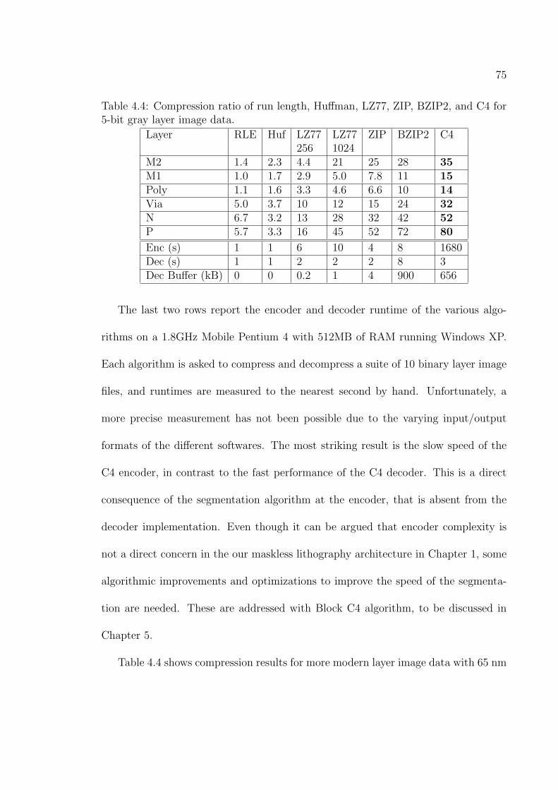
75

Table 4.4: Compression ratio of run length, Huffman, LZ77, ZIP, BZIP2, and C4 for5-bit gray layer image data.

Layer RLE Huf LZ77 LZ77 ZIP BZIP2 C4256 1024

M2 1.4 2.3 4.4 21 25 28 35M1 1.0 1.7 2.9 5.0 7.8 11 15Poly 1.1 1.6 3.3 4.6 6.6 10 14Via 5.0 3.7 10 12 15 24 32N 6.7 3.2 13 28 32 42 52P 5.7 3.3 16 45 52 72 80

Enc (s) 1 1 6 10 4 8 1680Dec (s) 1 1 2 2 2 8 3Dec Buffer (kB) 0 0 0.2 1 4 900 656

The last two rows report the encoder and decoder runtime of the various algo-

rithms on a 1.8GHz Mobile Pentium 4 with 512MB of RAM running Windows XP.

Each algorithm is asked to compress and decompress a suite of 10 binary layer image

files, and runtimes are measured to the nearest second by hand. Unfortunately, a

more precise measurement has not been possible due to the varying input/output

formats of the different softwares. The most striking result is the slow speed of the

C4 encoder, in contrast to the fast performance of the C4 decoder. This is a direct

consequence of the segmentation algorithm at the encoder, that is absent from the

decoder implementation. Even though it can be argued that encoder complexity is

not a direct concern in the our maskless lithography architecture in Chapter 1, some

algorithmic improvements and optimizations to improve the speed of the segmenta-

tion are needed. These are addressed with Block C4 algorithm, to be discussed in

Chapter 5.

Table 4.4 shows compression results for more modern layer image data with 65 nm

76

pixels and 5-bit gray layer image data. For each layer, 5 blocks of 1024× 1024 pixels

are sampled from two different layouts, 3 from the first, and 2 from the second, and the

minimum compression ratio achieved for each algorithm over all 5 samples is reported.

The reason for using minimum rather than the average has to do with limited buffering

in the actual hardware implementation of maskless lithography writers. Specifically,

the compression ratio must be consistent across all portions of the layer as much as

possible. From left to right, compression ratios are reported in columns for a simple

run-length encoder, Huffman encoder, LZ77 with a history buffer length of 256, LZ77

with a history buffer length of 1024, ZIP, BZIP2, and C4. Clearly, C4 still has the

highest compression ratio among all these techniques. Some notable lossless gray-pixel

image compression techniques have been excluded from this table including SPIHT

and JPEG-LS. Our previous experiments in [2] have already shown that they do not

perform well as simple ZIP compression on this class of data.

Again, the last two rows report the encoder and decoder runtime of the various

algorithms on a 1.8GHz Mobile Pentium 4 with 512MB of RAM running Windows

XP. Each algorithm is asked to compress and decompress a suite of 10 gray layer

image files, and runtimes are measured to the nearest second by hand. Again, the

slow speed of the C4 encoder contrasts the fast performance of the C4 decoder.

In Table 4.5, we show results for 10 sample images from the data set used to obtain

Table 4.4, where each row is information on one sample image. In the first column

“Type”, we visually categorize each sample as repetitive, non-repetitive, or containing

77

Table 4.5: Percent of each image covered by copy regions (Copy%), and its relationto compression ratios for Linear Prediction (LP), ZIP, and C4 for 5-bit gray layerimage data.

Type Layer LP ZIP C4 Copy%Repetitive M1 3.3 7.8 18 94%

Poly 2.1 6.6 18 99%Non-Rep. M1 14 12 16 18%

Poly 7.3 9.6 14 42%Mixed M1 7.5 12 15 44%

Poly 4.1 10 14 62%M2 15 26 35 33%N 18 32 52 21%P 29 52 80 33%Via 7.1 15 32 54%

a mix of repetitive and non-repetitive regions. The second column is the chip layer

from which the sample is drawn. The third column “LP” is the compression ratio

achieved by linear prediction alone, equivalent to C4 compression with copy regions

disabled. The fourth and fifth columns are the compression ratio achieved by ZIP

and the full C4 compression respectively. The last column “Copy%” is the percent of

the total sample image area covered by copy regions, when C4 compression is applied.

Any pixel of the image not covered by copy regions is, by default, linearly predicted

from its neighbors.

Clearly, the Copy% varies dramatically from image to image ranging from 18%

to 99% across the 10 samples, testifying to C4’s ability to adapt to different types of

layouts. In general a high Copy% corresponds to repetitive layout, and low Copy%

corresponds to non-repetitive layout. Also, the higher the Copy%, the more favor-

ably ZIP compares to LP compression. This agrees with the intuition that LZ-style

78

techniques work well for repetitive layout, and prediction techniques work well for

non-repetitive layout. At one extreme, in the non-repetitive-M1 row, where 18% of

the image is copied in C4, LP’s compression ratio exceeds ZIP. At the other extreme,

in the repetitive-Poly row, where 99% of the image is copied, ZIP’s compression ratio

is more than 3 times that of LP. In some cases, the compression ratio becomes high for

both LP and ZIP, e.g. the rows labeled Mixed-N and Mixed-P. These layouts contain

large featureless areas, which are easily compressible by both copying and prediction.

In these cases, C4 favors using prediction to avoid the overhead of specifying copy

parameters.

4.7 Tradeoff Between Memory and Compression

Efficiency

Compression algorithms, in general, require the use of a memory buffer at the de-

coder to store information about the compressed data. In general, larger buffers allow

more information to be stored, which may lead to higher compression ratios. On the

other hand, the size of this buffer, which must be implemented in decoder hardware,

has a direct impact on implementation complexity. For copy-based compression al-

gorithms, such as C4, LZ77, and ZIP, the buffer stores previously decoded data to

copy from. For BZIP2, the buffer stores the block of data over which block-sorting

is performed. For simpler schemes such as Huffman coding, the buffer stores symbol

79

statistics and the code table. For the very simple run-length code, the buffer stores

the current symbol being repeated, and the number of remaining repetitions.

In C4, most of the decoder buffer is used to support the copy operations; after

all, data cannot be copied unless it is stored somewhere accessible. Copying from

above requires storing multiple rows of image data at the decoder to enable the copy

operation. To allow copies from 1 to maxdy pixels above, the decoder needs buffering

to store the current row, and maxdy rows above, for a total of maxdy + 1 rows.

Clearly, increasing maxdy potentially allows more copy regions to be discovered.

However each stored row requires image width × bits per pixel = bits per row bits

of buffering. Total decoder buffering is bits per row ×(maxdy + 1) + constant where

the constant is used as overhead to support other aspects of C4, i.e. prediction,

decoding copy regions. For the 1024× 1024 image with 5-bit gray pixels used in our

experiments, bits per row is 5120 bits or 640 bytes, and the constant is 3410 bits or

427 bytes.

Using the same Poly layer layer image data as in Table 4.4, i.e. modern layer

image data with 65 nm pixels and 5-bit gray levels, we tested C4 with 2, 32, 64, 128,

256, 1024 stored rows, corresponding to total decoder buffer of 1.7 kB, 21 kB, 41 kB,

82 kB, 164 kB, 656 kB, respectively. Results of the tradeoff between decoder buffer

and compression ratio for C4, as compared to run-length, Huffman, LZ77, ZIP, and

BZIP2, are shown in Figure 4.10.

The x-axis is the decoder buffer size plotted on a logarithmic scale, and the y-axis

80

1

3

5

7

9

11

13

15

1 10 100 1000 10000 100000 1000000Decoder Memory (bytes)

Min C

ompr

essio

n Rati

o on P

oly La

yer RLE

HuffmanLZ77ZIPBZIP2C4Block C4

Figure 4.10: Tradeoff between decoder memory size and compression ratio for variousalgorithms on Poly layer.

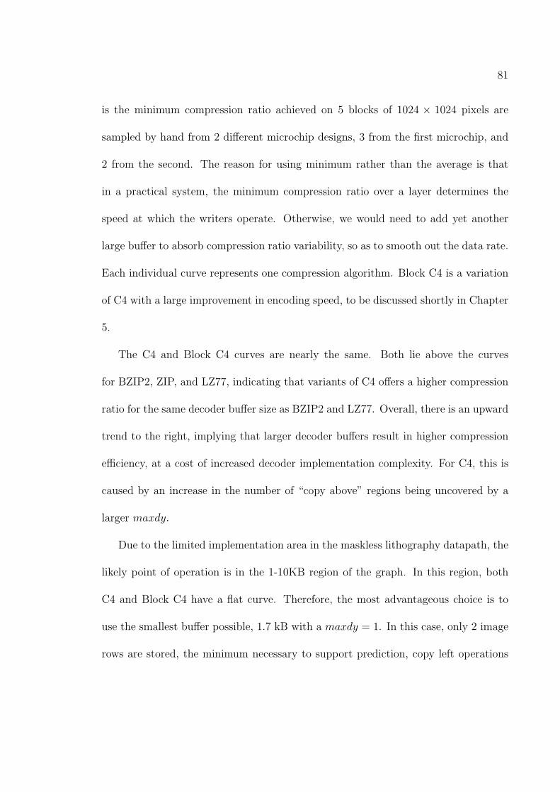
81

is the minimum compression ratio achieved on 5 blocks of 1024 × 1024 pixels are

sampled by hand from 2 different microchip designs, 3 from the first microchip, and

2 from the second. The reason for using minimum rather than the average is that

in a practical system, the minimum compression ratio over a layer determines the

speed at which the writers operate. Otherwise, we would need to add yet another

large buffer to absorb compression ratio variability, so as to smooth out the data rate.

Each individual curve represents one compression algorithm. Block C4 is a variation

of C4 with a large improvement in encoding speed, to be discussed shortly in Chapter

5.

The C4 and Block C4 curves are nearly the same. Both lie above the curves

for BZIP2, ZIP, and LZ77, indicating that variants of C4 offers a higher compression

ratio for the same decoder buffer size as BZIP2 and LZ77. Overall, there is an upward

trend to the right, implying that larger decoder buffers result in higher compression

efficiency, at a cost of increased decoder implementation complexity. For C4, this is

caused by an increase in the number of “copy above” regions being uncovered by a

larger maxdy.

Due to the limited implementation area in the maskless lithography datapath, the

likely point of operation is in the 1-10KB region of the graph. In this region, both

C4 and Block C4 have a flat curve. Therefore, the most advantageous choice is to

use the smallest buffer possible, 1.7 kB with a maxdy = 1. In this case, only 2 image

rows are stored, the minimum necessary to support prediction, copy left operations

82

and copying from immediate row above.

83

Chapter 5

Block C4 - A Fast Segmentation

Algorithm for C4

Block C4 is an improvement to the Context Copy Combinatorial Coding (C4)

compression algorithm described in Chapter 4. It provides about the same compres-

sion efficiency as C4 but at a tiny fraction of the encoding time. How large is the

speedup? In Table 5.1, we compare the compression efficiency and encoding time

of two 1024 × 1024 5-bit grayscale layer images, generated from two different sec-

tions of the poly layer of an industry microchip. In columns, from left to right, are

the layer image name, C4 compression ratio, C4 encode time, Block C4 compression

ratio, and Block C4 encode time. Both C4 and Block C4 use the smallest 1.7 kB

buffer, corresponding to only 2 stored rows of data. Encoding times are generated

on an Athlon64 3200+ Windows XP desktop with 1 GB of memory. A quick glance

84

Table 5.1: Comparison of compression ratio and encode times of C4 vs. Block C4.

Image C4 C4 Block C4 Block C4Comp. Ratio Encode Time Comp. Ratio Encode Time

Poly-memory 7.60 1608 s 7.63 14s(26.8 min) (115x speedup)

Poly-control 9.18 12113 s 9.18 13.9s(3.4 hrs) (865x speedup)

at this table reveals the speed advantage of Block C4, i.e. 115 times faster for the

Poly-memory image, and 865 times faster on the Poly-control image with no loss in

compression efficiency. There are some images for which BlockC4 has significantly

lower compression efficiency, but the speed advantage is universal. A more complete

table of results appears in Section 5.4 of this chapter.

The significance of a speedup of this magnitude in encoding time cannot be un-

derstated. Indeed, if we extrapolate from an average encoding time of 30 minutes per

1024 × 1024 layer image, a 20 mm × 10 mm chip die with drawn on a 25 nm 5-bit

grayscale grid would take over 18 CPU years to encode. Block C4 reduces this to

number to 49 CPU days, still a large number, but manageable by today’s multi-CPU

compute systems. Another benefit of Block C4, less readily apparent, is a constant

computation time of 14 s per 1024× 1024 layer image, independent of the layer data,

as compared to widely varying computation times of C4, from 27 minutes to 3.4 hours

in Table 5.1. A predictable and consistent computation time is important to project

planners managing the overall data processing flow, for example, when planning jobs

to maximize tool usage.

The remainder of this chapter describes how Block C4 achieves this encoding

85

speed up with little or no loss to compression efficiency. In Section 5.1, we introduce

the segmentation algorithm of C4 and contrast it with Block C4. In Section 5.2, we

examine the problem of choosing a block size for Block C4. In Section 5.3, we describe

how the Block C4 segmentation is encoded for compression efficiency.

5.1 Segmentation in C4 vs. Block C4

The basic concept underlying both C4 and Block C4 compression is exactly the

same. Layer data is characterized by a heterogenous mix of non-repetitive and repeti-

tive structures, examples of which are previously shown in Figures 4.2 and 4.3 respec-

tively. Repetitive structures are better compressed using Lempel-Ziv (LZ) style copy-

ing, whereas non-repetitive structures are better compressed using localized context-

prediction techniques, as described in Chapter 4. The task of both the C4 and Block

C4 encoder is to automatically partition the image between repetitive copy regions,

and non-repetitive prediction regions, in a process called segmentation. The resulting

segmentation map indicates which algorithm should be used to compress each pixel

of the image, i.e. either copy or prediction. Once the segmentation is complete, it

becomes a simple matter to encode each pixel according to this segmentation map.

The segmentation must also be encoded and included as part of the compressed data,

so that the decoder can know which algorithm to apply to each pixel for decoding.

In fact, the task of computing this segmentation accounts for nearly all the compu-

tation time of the C4 encoder. Of the encode times reported in Table 5.1, the encode

86

time excluding segmentation, is a constant 1.2 seconds, for C4 and Block C4. In

other words, over 99.9% of the encode time of C4 and 91% of the encode complexity

of Block C4 is attributable to segmentation. Why is segmentation such a complicated

task? To answer this question, we need to understand segmentation algorithm for

both C4 and Block C4.

In C4, the segmentation is described as a list of rectangular copy regions. An

example of a copy region is shown previously in Figure 4.4. Recall that each copy

region is a rectangle, enclosing a repetitive section of layer, described by 6 values, the

rectangle position (x, y), width and height (w, h), the direction of the copy (dir =

left/above), and the distance to copy from (d) i.e. the period of the repetition.

What makes automated C4 segmentation such a complex task is that the “best”

segmentation, or even a “good” segmentation is hardly obvious. Even in such a

simple example shown in Figure 4.4, there are many potential copy regions, a few of

which are illustrated in Figure 5.1 as colored rectangles, e.g the dashed blue rectangle

and a dot-dashed orange rectangle. Assuming a N × N pixel image, the number of

all possible copy regions is O(N5), where each copy region parameter (x, y, w, h, d)

contributes one O(N). Then, choosing the best set of copy regions for a given image

is a combinatorial problem. Exhaustive search on this space is prohibitively complex,

and C4 already adopts a number of greedy heuristics to make the problem tractable,

as described in Chapter 4. However, clearly further complexity reduction of the

segmentation algorithm is desirable, for all the reasons we have already described at

87

Figure 5.1: Illustration of alternative copy region.

the start of this chapter.

Block C4 adopts an entirely different segmentation algorithm from C4, which is

far more restrictive, and therefore much faster to compute. Specifically, C4 allows

for copy regions to be placed in arbitrary (x, y) positions with arbitrary (w, h) sizes

whereas Block C4 restricts both the position and sizes to fixed M × M blocks on

a grid. Figures 5.2 and 5.3 illustrate the difference between Block C4 and C4 seg-

mentation. In Figure 5.2, the segmentation for C4 is composed of 3 rectangular copy

regions, with 6 values (x, y, w, h, dir, d) describing each copy region. In Figure 5.3, the

segmentation for Block C4 is composed of 20 M ×M tiles, with each tile marked as

either prediction (P), or the copy direction and distance (dir, d). This simple change

reduces the number of possible copy regions to O(N3/M2), i.e. N2/M2 blocks times

O(N) variations on (dir, d), a substantial N2M2 reduction in search space compared

to C4. For the experiment in Table 5.1, N = 1024 and M = 8, so the copy region

search space has been reduced by a factor of 64 million. However, this complexity

reduction potentially comes at some cost to compression efficiency.

88

x1,y1,w1,h1 dir1,d1

x3,y3,w3,h3 dir3,d3

x2,y2 w2,h2 dir2,d2

Figure 5.2: C4 Segmentation

dir1

d1 ,2

dir2

d2

P

dir2

d2 dir2

d2

dir1

d1

dir1

d1

dir1

d1 dir1

d1 dir1

d1

P

P

dir3

d3 dir3

d3

dir3

d3 dir3

d3

P

P

P

P

M

M

Figure 5.3: Block C4 Segmentation.

89

5.2 Choosing a block size for Block C4

Comparing the segmentation of C4 in Figure 5.2 to Block C4 in Figure 5.3, we

see that what was once 3 large copy regions has been divided into 13 small square

blocks in this example. In general, a large repetitive w × h region is broken up

into approximately wh/M2 tiles in Block C4. Even though each copy region tile in

BlockC4 is represented with only 2 values (dir, d), whereas each copy region in C4

is represented with 6 values (x, y, w, h, dir, d), if a sufficiently large region is broken

up into tiles, there might be a net increase in the amount of data needed to store

the segmentation information. This extra data translates into lower compression

ratios. Smaller values of M accentuate this effect, motivating the use of larger M ;

however, larger values of M cause the following quantization problem: Comparing the

segmentation of C4 in Figure 5.2 to Block C4 in Figure 5.3, we see that the rectangles

are forced to snap to the coarse grid in Block C4. In C4, the rectangle boundaries are

optimized in order to separate repetitive regions from non-repetitive regions. In Block

C4, the coarse grid causes this separation to be sub-optimal. Consequently, at the

boundary of the copy regions, we might observe repetitive regions which are predicted,

and non-repetitive regions which are copied. This sub-optimal segmentation lowers

the compression efficiency. Of course, the smaller and finer the grid, the less grid

snapping occurs, motivating the use of a smaller M .

These arguments would suggest that there is an optimal M value that trades off

between grid snapping and the breakup of large copy regions. Empirically, we have

90

found among the values of M = 4, M = 8, and M = 16, M = 8 exhibits the best

compression efficiency for nearly all test cases. The reason for this requires further

investigation and is outside the scope of this thesis. Our Block C4 algorithm offers

the block size as a tunable parameter. In this thesis, we set M = 8 for Block C4

unless otherwise specified.

5.3 Context-based block prediction for encoding

Block C4 segmentation

To further improve the compression efficiency of Block C4, we note that the seg-

mentation shown in Figure 5.3 is highly structured. Indeed, consider that the seg-

mentation represents boundaries in a layer image separating repetitive regions from

non-repetitive regions, and that these repetitions are caused by design cell hierarchies,

which are placed on an Manhattan grid. Consequently, Block C4 segmentation has an

Manhattan structure, and C4 already employs a reasonable method for compressing

Manhattan structures placed on a grid, namely context-based prediction.

To encode the segmentation, blocks are treated as pixels, and the (P, dir, d) triplet

as a “color”. The value of the triplet z = (P, dir, d)z is predicted from its 3-block

neighborhood a = (P, dir, d)a, b = (P, dir, d)b, and c = (P, dir, d)c, as shown in

Figure 5.4. The prediction formula is the following conditional: if(c = a)thenz =

b, elsez = c. For vertical copy region boundaries, it is true that c = a and z =

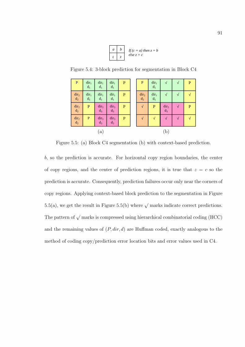
91

a b

c z

If (c = a) then z = b else z = c

Figure 5.4: 3-block prediction for segmentation in Block C4

dir1

d1 ,2

dir2

d2

P

dir2

d2 dir2

d2

dir1

d1

dir1

d1

dir1

d1 dir1

d1 dir1

d1

P

P

dir3

d3 dir3

d3

dir3

d3 dir3

d3

P

P

P

P

dir1

d1 ,2

dir2

d2

P

√

√

√ √

dir1

d1 √

√

P

√

dir3

d3

√

√

√

√

P

√

P

(a) (b)

Figure 5.5: (a) Block C4 segmentation (b) with context-based prediction.

b, so the prediction is accurate. For horizontal copy region boundaries, the center

of copy regions, and the center of prediction regions, it is true that z = c so the

prediction is accurate. Consequently, prediction failures occur only near the corners of

copy regions. Applying context-based block prediction to the segmentation in Figure

5.5(a), we get the result in Figure 5.5(b) where√

marks indicate correct predictions.

The pattern of√

marks is compressed using hierarchical combinatorial coding (HCC)

and the remaining values of (P, dir, d) are Huffman coded, exactly analogous to the

method of coding copy/prediction error location bits and error values used in C4.

92

5.4 Compression results for Block C4

As we have seen in the previous sections, Block C4 speeds up C4 by introducing a

coarse fixed grid of M×M pixel blocks for the segmentation. This change dramatically

reduces the size of the search space for copy regions, resulting in a large speedup of the

encoding time. In general, the coarse grid results in lowered compression efficiency,

but we have tuned the block size, and applied context-based block prediction to

reduce this effect. The full table of results, comparing Block C4 to C4 is shown in

Table 5.2. In it, we compare the compression efficiency and encoding time of various

1024 × 1024 5-bit grayscale images, generated from different sections and layers of

an industry microchip. In columns, from left to right, are the layer image name, C4

compression ratio, C4 encode time, Block C4 compression ratio, and Block C4 encode

time. Both C4 and Block C4 use the smallest 1.7 kB buffer, corresponding to only 2

stored rows of data. Encoding times are generated on an Athlon64 3200+ Windows

XP desktop with 1 GB of memory.

A quick glance at this table makes clear the speed advantage of Block C4 over

C4 is universal, over 100 times faster than C4, for images of all layers and sections of

layout tested. In general, the compression efficiency of Block C4 matches that of C4.

One exception is row 5 of Table 5.2, where C4 significantly exceeds the compression

efficiency of Block C4, on the highly regular M1-memory layer image.

On this image, C4’s compresssion ratio is 13.1, while Block C4’s compression

ratio is 9.5. The reason is that in this particular case, the layout of the polygons is

93

Table 5.2: Comparison of compression ratio and encode times of C4 vs. Block C4 for1024× 1024, 5 bpp images.

Image C4 C4 Block C4 Block C4Comp. Ratio Encode Time Comp. Ratio Encode Time

Poly-memory 7.60 1608 s 7.63 14s(26.8 min) (115x speedup)

Poly-control 9.18 12113 s 9.18 13.9s(3.4 hrs) (865x speedup)

Poly-mixed 10.59 1523 s 11.35 13.9s(25.4 min) (110x speedup)

M1-memory 13.1 3841 s 9.50 13.9s(1.1 hrs) (276x speedup)

M1-control 18.7 13045 s 17.3 13.9s(3.6 hrs) (938x speedup)

M1-mixed 15.5 13902 s 14.7 13.9s(3.9 hrs) (1000x speedup)

Via-dense 10.2 3350 s 15.5 14.1s(55.8 min) (237x speedup)

Via-sparse 16.0 7478 s 21.6 13.7s(2.1 hrs) (546x speedup)

extremely repetitive, and C4 covers 99% of the entire 1024 × 1024 image with only

132 copy regions. Moreover, many of these copy regions are long narrow strips, less

than 8-pixels wide, which Block C4 cannot possibly duplicate. Consequently, Block

C4 exhibits a significant loss of compression efficiency as compared to C4, in this

particular case.

On the other hand, in the last two rows of Table 5.2, the compression ratio of

Block C4 significantly exceeds the compression ratio of C4 for the dense and sparse

Via layer images. The reason for this is that the Via layer consists of a large number

of small squares scattered like flakes across the image. It is best compressed with a

large number of small copy regions, each covering a few squares. Block C4 has two

94

advantages in this case: first, it uses fewer bits to represent each copy region than C4;

second, it takes advantage of correlations between copy regions, using context-based

block prediction. For example, in the Via-sparse layer image, C4 applies 945 copy

regions to cover only ≈ 50% of the layout. In contrast, BlockC4 covers ≈ 96% of

the same image with copy regions, thereby achieving significantly higher compression

ratio.

95

Chapter 6

Full Chip Characterizations of

Block C4

From the results of the previous chapter, it is clear that Block C4 enjoys several

advantages over C4. First, its encoding time is 2 orders of magnitude faster than

C4. Second, its run time is consistently predictable; all the variations in speedup in

Table 5.2 come from wildly varying runtimes in C4. Third, its compression ratio is

comparable, if not equal to that of C4.

With the speedup and consistent runtimes provided by Block C4, it becomes

reasonable to consider runs on full chip, multi-layer layouts, something that remains

nearly impossible to do for C4. In these next set of experiments, we re-examine

the comparison between Block C4, ZIP, and BZIP2, only this time, statistics are

presented for a full production industry microprocessing chip, rather than individual

96

images sampled here and there across a chip.

The layout used for these calculations are for an industry standard microprocessor

designed for the 65nm device generation. The specifications for manufacturing this

design is shown in Table 6.1. The layout is 8.3mm × 14.1mm in size with polygons

laid out on a 1nm grid. The appropriate pixel size for this generation is 32nm×32nm,

with 33 (0-32) levels of gray to achieve 1nm edge placement control, which requires

6-bits per pixel. The computed rasterized pixel image data is 2.1 Tb per chip layer,

241 Tb per wafer layer. The manufacturing throughput requirement for lithography

is 1 wafer layer per 60s. Therefore, the required average maskless lithography data

rate over one wafer layer is 4.0 Tb/s.

This data rate is 1/3 the 12 Tb/s we have projected in Table 1.1 for two rea-

sons. First, this microprocessor is a 65 nm chip design, and as such, its pixel size is

(65/45)2 = 2 times larger in area than that of a 45 nm chip. A 2× larger pixel means

1/2 the number of pixels per unit area, and therefore, 1/2 the data per unit area.

Second, this microprocessor is only 8.3mm × 14.1mm = 117mm2 which is approxi-

mately 2/3 the size of the 10mm× 20mm = 200mm2 chip, as assumed in Table 1.1.

The combination of these two factors, a larger device generation, and a smaller chip

design, accounts for the 1/2× 2/3 = 1/3 reduction in data rate, as compared to the

data rate in Table 1.1.

In previous chapters, individual layout clips are characterized as dense, sparse,

repetitive, and non-repetitive, with each term intuitively defined by visual inspection.

97

Table 6.1: Specifications for an industry microprocessor designed for the 65nm devicegeneration.

Manufacturing specifications Maskless lithography specificationsMinimum feature 65 nm Pixel size 32 nmEdge placement 1 nm Pixel depth 6 bits (0-32) grayChip size 8.3 mm × 14.1 mm Pixel data 689 Gb

(one chip layer)Wafer size 300 mm Wafer data 241 Tb

(one wafer layer)Wafer throughput 1 wafer per 60s Average data 4.0 Tb/s over(one layer) throughput one wafer layer

This manual ad hoc characterization does not scale to a full chip run. Instead, we

define here a metric for polygon complexity which intuitively matches to the concept

of “dense”, namely the number of polygon vertices within a given area, or vertex

density. If the number of vertices is large in a fixed area, then it must be caused

by either the presence of many distinct polygons, or polygons with very complex

fragmented edges. In either case, for the simple 3-pixel prediction mechanism used

by C4 and BlockC4, the number of vertices is directly correlated with the number of

context-based prediction errors, as we have shown previously in Section 4.2.

In terms of repetitions, it is difficult to find a single metric that decisively deter-

mines this for a 2D image and that is reasonable to compute for such a large data

set. One method would have been to use the same search based segmentation used by

LZ77/C4 itself, but this defeats the purpose of having an independent metric. Other

techniques evaluated, such as image correlation, window-based DCT do not correlate

well with the copy mechanism of C4 and LZ77 where the cost of even correcting a

small 1% intensity error is fairly high. Such techniques are more appropriate for lossy

98

Figure 6.1: A vertex density plot of poly gate layer for a 65nm microprocessor.

compression techniques where such errors may be ignored. In the end, we choose

to use a metric taken from the layout hierarchy itself. The measure of repetition is

defined as the number of cells in a given region, minus the number of unique cells in

that same region. As an example, suppose a region contains 5 instances of cell A, 4

instances of cell B, and 1 instance of C, D, and E. Then the total number of cells in

that region is 5 + 4 + 1 + 1 + 1 = 12 whereas the total number of unique cells is 5

(A-E), so the “repetition” of this region is 7.

In order to provide a visualization of the these metrics, Figure 6.1 shows a grayscale

picture of the vertex density metric as applied to the poly gate layer. Each pixel in this

picture corresponds to a 32µm×32µm block of the chip. Vertex densities range from

0 to 20,000 per block. Higher vertex density blocks are assigned brighter pixels, and

99

lower corner vertex density blocks are assigned darker pixels. It is easy to discern from

this image regions of very high vertex densities that are arranged in rectangular arrays

throughout the design. These are the various memory arrays of the microprocessor.

The darker grays are likely to be logic circuit areas, also arranged in rectangular

arrays. Finally, the periphery regions are very dark, indicating low corner densities.

A plot of “repetitions” visually looks the same as Figure 6.1. Although there

are small differences in the data which are detectable through data analysis, it is

impossible to visually discern these differences. The visual similarity between a plot

of “repetitions” and a plot of vertex density justifies the fundamental rationale behind

C4. Highly dense layout regions are also highly repetitive, and therefore compress

well with copying techniques. Non-repetitive regions tend to be sparse, and hence

compress well with context based prediction techniques, as polygon corners generally

correspond to prediction errors for Manhattan geometries.

As a point of comparison, the vertex density plot of Metal1 is shown in Figure

6.2. Although there are a few discernable differences, for the most part, Figures 6.1

and 6.2 look very similar as well.

For each of the 32µm×32µm blocks, rasterization is performed using the method-

ology described in Chapter 2, where the pixel size is 32nm, and 33 gray levels are

allowed (0-32) resulting in a fine 1nm edge placement grid. One full chip layer con-

tains 116,328 such blocks, equal to the number of pixels in Figure 6.1. Each rasterized

block is then passed through 3 compression algorithms, ZIP, BZIP2, and Block C4

100

Figure 6.2: A vertex density plot of Metal1 layer for a 65nm microprocessor.

and compression and decompression statistics are gathered for each. This process is

then repeated for all the critical layers of the design: diffusion, also known as active,

poly, contact, metal1, via1 and metal2.

For this experiment, decoder buffer size of ZIP, BZIP2 and Block C4 are 4kB,

900 kB, and 1.7 kB respectively, chosen based on the tradeoff analysis presented in

Section 4.7. The small buffer size used by Block C4 makes it particularly attractive

for implementation in hardware for the datapath architecture presented in Chapter

1.

101

6.1 Full chip compression statistics

Table 6.2 contains a summary of these full chip runs. Column 1 is the name of

the full-chip statistic being reported. Column 2 is the chip layer which is rasterized

and compressed. Columns 3, 4, and 5 are the statistics for ZIP, BZIP2 and Block

C4 respectively. Each row in the table represents a layer statistic. The relevant

statistics reported are the average compression ratio for the entire layer, the minimum

compression ratio over individual 32µm× 32µm blocks, the total encoding run time

for each layer, the total decoding run time for each layer, and the percentage of blocks

with compression ratio below 10.

Examining the average compression ratio for all layers, the compression efficiency

of ZIP is generally lower than that of BZIP2 and Block C4. BZIP2 and Block C4 are

generally comparable to each other. Considering that BlockC4 uses 2 or 3 orders of

magnitude less decoder buffer to achieve more or less the same compression efficiency

as BZIP2, clearly it is the algorithm of choice for hardware implementation. From

layer to layer, Metal1 is most challenging to compress, followed by Metal2, Via1, Poly,

Contact, then Active. One different characteristic of Poly layout in this particular

design style is that all gates are oriented in a single direction, and are spaced apart by

a characteristic common pitch. Regularized design styles such as these can take better

advantage of the copy mechanism in C4 to achieve high compression efficiency. Of

particular concern is the average compression ratio of the Metal1 and Metal2 layers

which are 5.2 and 7.2 respectively, which fall below the target compression ratio of

102

Table 6.2: Full-chip compression summary table.

Statistic Layer ZIP BZIP2 Block C4Avg. Compression Ratio Poly 12.6 15.3 14.1

Metal1 4.2 4.5 5.2Metal2 6.1 7.2 7.2Contact 14.1 16.0 23.2Active 20.2 31.7 39.2Via1 12.3 14.1 14.0

Min. Compression Ratio Poly 2.6 3.1 4.4Metal1 0.96 1.3 1.7Metal2 1.0 1.3 2.1Contact 2.7 4.3 4.8Active 8.1 11.1 12.8Via1 2.2 3.6 4.5

Total Encoding Time Poly 42 min 2.3hrs 420 hrsMetal1 45 min 2.3hrs 420 hrsMetal2 45 min 1.9hrs 408 hrsContact 46 min 2.1hrs 419 hrsActive 43 min 1.9hrs 418 hrsVia1 46 min 2.1hrs 419 hrs

Total Decoding Time Poly 17 min 1.2hrs 36 minMetal1 14 min 1.2hrs 35 minMetal2 19 min 1.4hrs 38 minContact 15 min 1.4hrs 38 minActive 15 min 1.3hrs 37 minVia 15 min 1.4hrs 38 min

Percentage of Blocks Poly 25.33% 22.84% 23.66%with Compression Metal1 65.73% 59.69% 55.12%Ratio Below 10 Metal2 44.20% 44.88% 41.95%(lower is better) Contact 0.73% 0.07% 0.00%

Active 7.85% 0.00% 0.00%Via 4.94% 0.22% 0.14%

103

10 presented in Chapter 1.

Another important metric to consider is the minimum compression ratio over all

32µm× 32µm blocks for a layer. This is the most difficult block of any given layer to

compress. In this case, only the Active layer meets a target compression ratio of 10.

The remaining 5 layers fall below that target, and in the worst case block of Metal1,

the compression ratio is 1.7.

6.2 Managing local variations in compression ra-

tios

So what are the implications of missing the compression target, and which is more

relevant, the average compression ratio, or the more pessimistic minimum compres-

sion ratio? The answer depends on how well the maskless lithography system as a

whole can absorb local variations in data throughput. This can be accomplished by

physically varying the throughput of the maskless lithography writers, or by intro-

ducing various mechanisms in the datapath to absorb these variations which we will

speculate on later. By local variations, we are referring to inter-block variations of

compression ratios. In choosing our block size for analysis, we already assume there is

at least a single block buffer in the system so that we may ignore intra-block variations

in compression ratio. This buffer is distinct from the memory used by the decompres-

sion hardware. An example of such a buffer is the “SRAM Writer Interface” found

104

in [39].

6.2.1 Adjusting board to chip communication throughput

In the worst case, (a) the maskless lithography writers are fixed at a constant

writing speed over all blocks of a layer; and (b) the datapath cannot help absorb

these inter-block variations of compression ratios. In this case, the writing speed

is limited by the data throughput of the minimum compression ratio block. From

the the maskless datapath presented in Chapter 1, the formula to compute actual

wafer throughput is rwafer = rcomm,max × Cmin/dwafer where rwafer is the wafer layer

throughput, rcomm,max is the maximum board to chip communication throughput,

Cmin is the minimum compression ratio for Block C4, and dwafer = 241 Tb is the

total data for one wafer layer, from Table 6.1.

Since dwafer is fixed and Cmin has been empirically determined for each layer, the

total wafer throughput depends entirely on rcomm,max which is the maximum data

throughput of board to chip communication. The reason maximum is emphasized is

that this throughput is only required for the minimum compression ratio block. For

blocks of higher compression ratio, the communication throughput can be reduced.

As an example, if maximum communication throughput rcomm,max = 1 Tb/s, then

the wafer layer throughput for Metal1 is 1 Tb/s × 1.7 / 241 Tb × 3600s/hr = 25.5

wafer layers per hour. This same formula can be applied to each layer for various

assumed values of rcomm,max. The results of this exercise are shown on Table 6.3.

105

Table 6.3: Maximum communication throughput vs. wafer layer throughput forvarious layers in the worst case scenario, when data throughput is limited by theminimum compression ratio for Block C4.

Layer Cmin rcomm,max(Tb/s) rwafer(wafer · layer/hr)Poly 4.4 1 65.7Metal1 1.7 1 25.5Metal2 2.1 1 31.4Contact 4.8 1 71.7Active 12.8 1 191Via1 4.5 1 67.2

Poly 4.4 0.91 60Metal1 1.7 2.36 60Metal2 2.1 1.91 60Contact 4.8 0.83 60Active 12.8 0.31 60Via1 4.5 0.89 60

The columns of Table 6.3 are layer, minimum compression ratio, maximum board

to chip communication throughput, and wafer layer throughput, respectively. In the

first 5 rows, we assume a maximum communication throughput of 1 Tb/s and com-

pute the wafer throughput for various layers. In the next 5 rows, we target a wafer

throughput of 60 wafer layers per hour, and compute the maximum communication

throughput needed to support this writing rate for each layer. As a point of refer-

ence, a state-of-the-art HyperTransport 3.0 (HT3) link offers 0.32 Tb/s maximum

throughput [40]. Examining Table 6.3 for Metal1 with a target wafer throughput of

60 wafers per hour, a maskless datapath requires at least d2.36/0.32e = 8 such links

to achieve the required communications throughput. Implementing 8 links is costly,

in terms of both circuit power dissipation and chip area [34] [23]. However, a chip

designer may be able to conserve power by taking advantage of the fact that the

106

Table 6.4: Average communication throughput vs. wafer layer throughput for variouslayers, computed using the average compression ratio for Block C4.

Layer Cmin rcomm,avg(Tb/s) rwafer(wafer · layer/hr)Poly 14.1 1 211Metal1 5.2 1 77.7Metal2 7.2 1 108Contact 23.2 1 347Active 39.2 1 586Via1 14.0 1 209

Poly 14.1 0.28 60Metal1 5.2 0.77 60Metal2 7.2 0.56 60Contact 23.2 0.17 60Active 39.2 0.10 60Via1 14.0 0.29 60

maximum communication throughput is only needed for a few blocks. The average

communication throughput, as we shall see shortly, is significantly lower.

The equation relating wafer throughput rwafer to average board to chip commu-

nication throughput rcomm,avg and average compression ratio Cavg is straightforward:

rwafer = rcomm,avg × Cavg/dwafer. To be precise, the average is computed over all

blocks of an wafer layer. Using this formula, we can relate wafer throughput to aver-

age communication throughput for various layers. The results are presented in Table

6.4. The columns are layer, average compression ratio, average board to chip com-

munication throughput, and wafer layer throughput, respectively. The first 5 rows

assume an average communications throughput of 1 Tb/s, and the next 5 rows target

a wafer throughput of 60 wafer layers per hour.

Since the average compression ratio is significantly higher than the minimum com-

pression ratio for all layers, the average communication throughput is also significantly

107

lower than the maximum communication throughput computed previously. Continu-

ing our previous example using a HT3 link as reference, for Metal1 with a target wafer

throughput of 60 wafers per hour, a maskless datapath requires only 0.77/0.32 = 2.4

links on average. So even though 8 links are required to accommodate the maximum

throughput, on average only 2.4/8 = 30% of the capacity is being used. The maskless

datapath can take advantage of this by powering down unused communication links

to conserve power. However, that still leaves an area cost of implementing 8 links in

the first place. What can be done to effectively smooth the data throughput so that

communication links can be utilized more effectively?

6.2.2 Statistical multiplexing using parallel decoders

An important feature to take advantage of is the opportunity to utilize averaging

inherent in the parallel design of the maskless lithography datapath. As described in

[41], the decoder in Figure 1.9 is implemented as a parallel array of decoder paths,

i.e. multiple blocks are being decoded simultaneously. In its simplest form, the com-

munication throughput is evenly divided among the parallel decoder paths. However,

additional logic, such as packet scheduling, can be implemented to allocate commu-

nications throughput to each decoder path based on need. As such, a decoder path

working on a block with low compression ratio is allocated more communication pack-

ets than a decoder path working on a block with high compression ratio. The result is

that inter-block variations in compression ratio is effectively statistically multiplexed

108

by the number of decoder paths in the system.

Suppose we have N decoder paths working in parallel on N adjacent blocks in a

row. In communication order, we form M frames of N blocks per frame, where MN ≥

116, 326. Statistical multiplexing effectively allows us to average the compression ratio

over each frame. We can then compute the minimum over all frames and denote this

value as Cmin,N . Note, that by definition Cmin,1 = Cmin and Cmin,116,328 = Cavg.

Cmin,N , rwafer and rcomm,max are related through this equation: rwafer = rcomm,max ×

Cmin,N/dwafer.

Using different values for N, we compute the Cmin,N and rcomm,max for Block C4,

Metal1, and a target throughput of 60 wafer layers per hour. These results are

summarized in Table 6.5. In columns are the number of decoder paths N, the mini-

mum frame compression ratio Cmin,N , the maximum board to chip communications

throughput rcomm,max, the wafer throughput rwafer, and the number of HT3 links

needed to support the communications throughput. Clearly, Cmin,N increases as the

number of decoder paths N increases. At N = 1000, Cmin,N = 4.9 which is very close

to Cavg = 5.2, demonstrating the strength of the statistical multiplexing approach.

The corresponding maximum communication throughput is 0.82 Tb/s which can be

met with d0.82/0.32e = 3 HT3 links.

109

Table 6.5: Effect of statistical multiplexing using N parallel decoder paths on BlockC4 compression ratio and communication throughput for Metal1.

N Cmin,N rcomm,max(Tb/s) rwafer(wafer · layer/hr) # of HT3 links1 1.7 2.36 60 82 2.3 1.74 60 610 2.5 1.60 60 5100 3.3 1.21 60 41000 4.9 0.82 60 3116,328 5.2 0.77 60 3

6.2.3 Adding buffering to the datapath

Another way to smooth the data throughput is to introduce a memory buffer at the

output of the communications channel before decompressing the data in Figure 1.9.

The resulting system resembles Figure 1.7, except the memory buffer is much smaller.

This buffer absorbs variations in data throughput caused by inter-block variations of

compression ratios. For blocks with high compression ratio, excess communication

throughput is used to fill the buffer. For blocks with low compression ratio, data is

drained from the buffer to supplement the communication channel. Intuitively, the

larger the buffer is, the more variations it can absorb, and the lower is the required

maximum communication throughput. On the other hand, the primary advantage

of spending area on a buffer in the first place is to save on chip area devoted to

communication. Therefore, there is a tradeoff between the area needed by the buffer

and the additional area saved by reducing the number of communication links.

We can roughly estimate the amount of buffer to add using the following steps.

Suppose we add sufficient buffer equivalent to the minimum compressed block. For

Metal1, this buffer is (1000 × 1000 × 6bits)/1.7 = 3.5Mb in size for Block C4. Now

110

suppose, in communication order, we group blocks pairwise and compute each pair’s

compression ratio, followed by computing the minimum over all pairs Cmin,pair. This

number is guaranteed to be higher than Cmin and lower than Cavg. Empirically for

Metal1, Cmin,pair = 2.3 for Block C4, assuming raster scan order. For this system, the

following inequality holds: rwafer ≥ rcomm,max×Cmin,pair/dwafer. That is, at the very

least, we should be able to replace Cmin with the higher Cmin,pair for relating wafer

throughput to the maximum communication throughput. Continuing our previous

example for Metal1 with a target wafer throughput of 60 wafers per hour, the result

is rcomm,max ≤ 1.74Tb/s, equivalent to d1.74/0.32e = 6 HT3 links. Compared with

the 8 HT3 links for zero buffering, this is a reduction of 2 links for 3.5Mb of buffering,

which seems to be worthwhile tradeoff. Clearly, more systematic analysis of such

tradeoffs are necessary for any future practical maskless lithography systems.

6.2.4 Distribution of low compression blocks

The computation of rcomm,max in the previous paragraph is a conservative upper

bound, in that it focuses on the worst case where low compression ratio blocks may

be clustered together. Thus, we require that any drain on the buffer caused by a

low compression ratio block to be immediately refilled by the adjacent block. If

low compression blocks are spread far apart from each other by coincidence, then

rcomm,max may be significantly lowered. Furthermore, if the writing system allows

for limited re-ordering of the blocks, then this could be used to intentionally spread

111

the low compression ratio blocks apart. As an example, some maskless lithography

systems are written in a step-and-scan mode, where multiple blocks form a frame

which is written in a single scan [41]. In this case, blocks may be re-ordered within a

frame to smooth the data rate.

Figure 6.3 is a visualization of the compression ratio distribution of Block C4 for

the Metal1 layer. Brighter pixels are blocks with low compression ratios and darker

pixels are blocks with high compression ratios. Notice that repetitive memory arrays

on the bottom half are relatively dim. Block C4 compresses these repetitive regions

effectively. The less regular, but relatively dense layout are clustered in distinct bright

regions in the middle. This geographic distribution should be taken into consideration

when deciding on the mechanism to smooth inter-block variations.

6.2.5 Modulating the writing speed

Another possibility is to modulate the writing speed of the maskless lithography

writers to match the inter-block variations in compression ratio. For example, it is

conceivable to divide blocks into discrete classes based on the range of compression

ratios they fall into. The lithography writers would then switch between a discrete

number of writing speeds depending on the class of block. The “high” compression

ratio blocks are written with “high” speed, whereas “low” compression ratio blocks

are written with “low” speed. Due to overhead in switching speeds, it may not be

feasible to vary the writing speed on a block-by-block basis. In this case, the writers

112

Figure 6.3: A visualization of the compression ratio distribution of Block C4 for theMetal1 layer. Brighter pixels are blocks with low compression ratios, while darkerpixels are blocks with high compression ratios. The minimum 1.7 compression ratioblock is marked by a white crosshair (+).

113

would change speed based on the minimum compression ratio within a contiguous

group of blocks.

Whichever mechanism is used to smooth the data throughput, the effectiveness

depends on the distribution of compression ratios across all blocks of a layer. Intu-

itively, the higher the number of low compression ratio blocks, the more difficult it is

to lower the maximum communication throughput. Let us examine the distribution

of these variations.

6.3 Distribution of compression ratios

Figure 6.4 shows the histogram of compression ratios for the full-chip Poly layer

for Block C4, C4, and BZIP2. The horizontal axis is the compression ratio bins

ranging from 0 to 40 in increments of 1. The vertical axis is the count of the number

of blocks which fall into each bin. The histogram of Block C4 is plotted in red

with diamond markers, BZIP2 in green with square markers, and ZIP in blue with

triangular markers. The first observation to be made about this histogram is that

the distribution of compression ratios is multi-modal and non-Gaussian. Second, note

that the distribution has an extremely long tail beyond 30. In general, layout contains

a large amount of blank regions filled by a few large polygons. The information content

in these regions are low, and compress easily.

An alternative view of the same data is presented in Figure 6.5. In this case, we

plot the cumulative distribution of blocks on the vertical axis, against the compression

114

Histogram

0

1000

2000

3000

4000

5000

6000

7000

0 5 10 15 20 25 30 35 40

Compression Ratio

Fre

quen

cy

Block C4

BZIP2

ZIP

Figure 6.4: Histogram of compression ratios for BlockC4, BZIP2, and ZIP for thePoly layer.

115

ratio on the horizontal axis. Figure 6.5 is essentially the normalized integral of the

plot in Figure 6.4. The cumulative distribution function (CDF) of the compression

ratio of Block C4 is plotted in red with diamond markers, BZIP2 in green with

square markers, and ZIP in blue with triangular markers. A point on the CDF curve

represents the percentage of blocks Y with compression ratio less than X. Generally

speaking, when the curve shifts to the right, the overall compression efficiency of a

layer is improved.

Of particular interest is compression ratio bins at the low end of the spectrum,

as these are our throughput bottlenecks. In Figure 6.5, 25.3% of ZIP blocks, 22.8%

of BZIP2 blocks, and 23.7% of Block C4 blocks have compression ratio less than 10.

Therefore, in the low end of the compression spectrum, Block C4 and BZIP2 have

about the same compression efficiency, and both have better efficiency than ZIP. In

addition, even though the reported minimum compression ratio in Table 6.2 for Block

C4 and BZIP2 are 4.4 and 3.1 respectively, the CDF curve clearly shows that very few

blocks have compression ratios less than 5. In fact, for this poly layer, only 7 of the

116,328 blocks have compression ratio’s less than 5 for Block C4 and BZIP2. These

7 blocks are clustered in 2 separate regions, and within a region no two blocks are

adjacent to each other. The total size for these 7 blocks compressed by Block C4 is

9.1 Mb. Therefore, if we have enough memory buffer to simply store all 7 compressed

blocks then we can effectively use 5 as the minimum compression ratio for Poly. On

the other hand, 2.8% ≈ 1800 of ZIP blocks have compression ratio less than 5. Since

116

0%

10%

20%

30%

40%

50%

60%

70%

80%

90%

100%

0 5 10 15 20 25 30 35 40

Compression Ratio

Cum

ulat

ive

Dis

trib

utio

n

BlockC4BZIP2ZIP

Figure 6.5: Cumulative distribution function (CDF) of compression ratios forBlockC4, BZIP2, and ZIP for the Poly layer.

117

there are more variations, the system has to work harder to absorb them.

An alternative to absorbing the variation is to re-examine the compression algo-

rithm to look for ways to compress these difficult blocks more efficiently. Figures

6.6 and 6.7 are samples of such hard to compress blocks for Poly and Metal1 layout.

The key observation to make is that these blocks are dense in polygon count, and yet

are not regular repeated structures, although some repetition does exist. Metal1 is

more dense and less repetitive, and therefore has significantly lower compression ratio

than Poly. Increasing the buffer size of BlockC4 from 1.7 kB to 656 kB does improve

the compression efficiency, but not by a commensurate amount. For the Poly block

in Figure 6.6, the Block C4 compression ratio improves from 4.4 to 5.1, and for the

Metal1 block in Figure 6.7, the Block C4 compression ratio improves from 1.7 to 1.9.

Another way to gauge the difficulty of compressing the blocks in Figures 6.6 and

6.7 is to compute the entropy. Entropy is the theoretical minimum average number of

bits needed to losslessly represent each pixel, assuming pixels are independently and

identically distributed. This assumption does not hold for layout pixel data. Nonethe-

less, entropy still serves as a useful point of reference. For Figure 6.6, the entropy is 3.7

bits per pixel (bpp) which corresponds to a compression ratio of 6bpp/3.7bpp = 1.6.

For Figure 6.7, the entropy is 4.8 bpp, which corresponds to a compression ratio of

6bpp/4.8bpp = 1.3. Huffman coding realizes a compression ratio very close to entropy:

1.6 and 1.2 for Figures 6.6 and 6.7 respectively.

Another alternative is to systematically change the layout so as to improve its

118

Figure 6.6: A block of the poly layer which has a compression ratio of 2.3, 4.0, and4.4 for ZIP, BZIP2, and Block C4 respectively.

119

Figure 6.7: A block of the M1 layer which has a compression ratio of 1.1, 1.4, and 1.7for ZIP, BZIP2, and Block C4 respectively.

120

0%

10%

20%

30%

40%

50%

60%

70%

80%

90%

100%

0 5 10 15 20 25 30 35 40

Compression Ratio

Cum

ulat

ive

Dis

trib

utio

n

BlockC4BZIP2ZIP

Figure 6.8: CDF of compression ratios for BlockC4, BZIP2, and ZIP for the Contactlayer.

121

0%

10%

20%

30%

40%

50%

60%

70%

80%

90%

100%

0 5 10 15 20 25 30 35 40

Compression Ratio

Cum

ulat

ive

Dis

trib

utio

n

BlockC4BZIP2ZIP

Figure 6.9: CDF of compression ratios for BlockC4, BZIP2, and ZIP for the Activelayer.

122

0%

10%

20%

30%

40%

50%

60%

70%

80%

90%

100%

0 5 10 15 20 25 30 35 40

Compression Ratio

Cum

ulat

ive

Dis

trib

utio

n

BlockC4BZIP2ZIP

Figure 6.10: CDF of compression ratios for BlockC4, BZIP2, and ZIP for the Metal1layer.

123

0%

10%

20%

30%

40%

50%

60%

70%

80%

90%

100%

0 5 10 15 20 25 30 35 40

Compression Ratio

Cum

ulat

ive

Dis

trib

utio

n

BlockC4BZIP2ZIP

Figure 6.11: CDF of compression ratios for BlockC4, BZIP2, and ZIP for the Via1layer.

124

0%

10%

20%

30%

40%

50%

60%

70%

80%

90%

100%

0 5 10 15 20 25 30 35 40

Compression Ratio

Cum

ulat

ive

Dis

trib

utio

n

BlockC4BZIP2ZIP

Figure 6.12: CDF of compression ratios for BlockC4, BZIP2, and ZIP for the Metal2layer.

125

compression efficiency. It is usually possible to preserve the same design intent using

a different physical layout. If the design can be made more “compression friendly” in

these difficult blocks, then the compression efficiency can be improved.

For completeness of analysis, Figures 6.8 to 6.11 show the CDF plots of Contact,

Active, Metal1, Via1, and Metal2 layers respectively. Examining these plots, Block

C4 clearly has higher compression efficiency for Contact, Active, and Metal1 layers

than both BZIP2 and ZIP. For the Via1 and Metal2 layers, the compression efficiency

of Block C4 is comparable to BZIP2, particularly in the region of compression ratios

less than 10. Both Block C4 and BZIP2 have higher efficiency than ZIP.

Comparing the curves between levels, clearly Metal1 is the most difficult to com-

press. For a given low compression ratio threshold, for example 5, Metal1 has the

largest percentage of blocks falling below that threshold, i.e. 24% for Block C4.

Metal2 follows with 0.81% for Block C4. The remaining layers contain no blocks

below that threshold. Table 6.6 lists the complete numbers for all layers and com-

pression algorithms using a low compression ratio threshold of 5. The reason Metal1

and Metal2 are particularly challenging is simple. These layers are the primary wiring

layers connecting device to device, and as anyone who has untangled cables behind

a personal computer can attest, wires quickly turn into a complex mess if not care-

fully managed. Intuitively, this means that the wiring layers tend to be more dense,

and less regular than the other chip design layers, making them the most difficult

to compress. The density of polygon corners makes it difficult for context predic-

126

Table 6.6: Percentage of blocks with compression ratio less than 5.

Statistic Layer ZIP BZIP2 Block C4Percentage of Blocks Poly 0.03% 0.00% 0.00%with Compression Metal1 44.63% 34.20% 23.72%Ratio Below 5 Metal2 4.33% 3.75% 0.81%(lower is better) Contact 0.02% 0.00% 0.00%

Active 0.00% 0.00% 0.00%Via 0.01% 0.00% 0.00%

tion to achieve good compression, and the irregularity of the design makes it difficult

for copying to achieve good compression. The Block C4 segmentation algorithm is

stuck between the proverbial rock and a hard place. Nonetheless, to the extent that

some compression has been achieved, the algorithm does benefit from having both

prediction and copying. As an example, turning off copying reduces the Block C4

compression ratio to 1.4 from 1.7 for the Metal1 block shown in Figure 6.7.

6.4 Excluding difficult, low compression results

Another question we can ask is, if we can exclude the 100 most difficult to compress

blocks out of 116,328 blocks, either via buffering or some other mechanism, what is

the minimum compression ratio for each layer? The result is shown in Table 6.7. For

Metal1, Metal2, and Active, there is little change. However, for Poly, Contact and

Via, there is a significant improvement. For these layers, the minimum compression

ratio is pessimistic due to a small number of special cases. If these small number of

variations can be absorbed by the maskless lithography system, or by systematically

altering the design to be more compression-friendly, the overall wafer throughput can

127

Table 6.7: Minimum compression ratio excluding the lowest 100 compression ratioblocks.

Statistic Layer ZIP BZIP2 Block C4Min. Compression Ratio Poly 2.6 3.1 4.4over all blocks Metal1 0.96 1.3 1.7

Metal2 1.0 1.3 2.1Contact 2.7 4.3 4.8Active 8.1 11.1 12.8Via1 2.2 3.6 4.5

Min. Compression Ratio Poly 4.1 5.2 5.2excluding the lowest Metal1 1.0 1.4 1.8100 compression Metal2 1.4 2.5 2.5ratio blocks Contact 8.1 10.0 19.8

Active 8.1 11.1 12.9Via 8.2 10.5 11.0

be improved significantly.

6.5 Comparison of encoding and decoding times

Examining the encoding times in Table 6.2, clearly ZIP is the fastest, BZIP2 is

about 3 times slower than ZIP, and Block C4 about 20 times slower than BZIP2.

Part of the reason that Block C4 is so much slower is the inherent complexity of the

Copy/Context prediction segmentation code, and another part is the lack of code

optimization. Unlike BlockC4, both ZIP and BZIP2 have been optimized in C code.

All 3 algorithms have fairly stable and predictable runtimes which are independent

of the layer. This is a significant advantage over the layer dependent and extremely

long runtimes of C4 we have seen previously.

Examining decoding times, ZIP is again the fastest, but here Block C4 is faster

128

than BZIP2 by a factor of 2. Considering Block C4’s decode buffer requirement is

2 orders of magnitude less than BZIP2, it is clearly the best choice for hardware

implementation. Block C4 is a highly asymmetric algorithm in terms of encoder

vs. decoder complexity because segmentation is not required by the decoder, and

consequently, its decoding speed is about 40 times faster than its encoding speed.

6.6 Discussion

In summary, the results of this chapter validate the observations of the previous

chapters on full chip layout. Overall, a lossless compression ratio of 10 has not been

met. Nonetheless, compression can play an important role in most layers, and its

shortcomings can be mitigated through careful engineering of the overall maskless

lithography datapath and design layout. In addition, Block C4 has shown itself as

a strong candidate for implementation in the maskless lithography datapath shown

in Chapter 1, with the lowest decoder buffering requirement of 1.7 KB, low decoder

complexity in software, high compression efficiency, and a reasonable and predictable

compression speed in software.

129

Chapter 7

Hardware Implementation of the

C4 Decoder

To use C4 compression in a maskless lithography datapath shown in Figure 1.9,

the C4 decoder must ultimately be implemented as ASIC circuitry built on the same

substrate as the array of writers, as described in Chapter 1. The first step in this

endeavor is to break down the C4 decoder algorithm into functional blocks. Sub-

sequently, each block needs to be refined, step-by-step, down to the gate level, and

finally the transistor level. In this chapter, we consider the first steps of breaking C4

down to functional blocks, and refining the blocks, in particular, the region decoder.

We begin with the high level block diagram of the C4 decoder for grayscale layer

images, shown previously in Figure 4.8. In Figure 7.1, we have slightly rearranged

Figure 4.8, to emphasize the inputs and outputs. The decoder has 3 main inputs:

130

error value

error location bits HCC Decoder

Predict/Copy Image Buffer

Error Merge

C4 Decoder

Huffman Decoder

Segmentation

Compressed error value

Compressed error bits

Writers

Inputs from C4 Encoder Output

pixels

Figure 7.1: Block diagram of the C4 decoder for grayscale images.

a segmentation, a compressed error location map, and a stream of compressed error

values. The segmentation is a list of copy regions, which indicate whether each pixel

is copied or predicted. The compressed error location map is a compressed stream

of bits, decompressed by the HCC Decoder block. Each bit in this stream controls

whether the Merge block accepts the Predict/Copy value, or the error value input.

The error value stream is generated by Huffman decoding the compressed error value

input. If the error location bit is 0, the Predict/Copy value is correct and is sent

as output to the writers. If the error location bit is 1, the Predict/Copy value is

incorrect, and the error value is sent as output to the writers. In addition, the output

to the writers is stored in a image buffer, to be used in the future for prediction or

copying.

Of the 5 blocks in the decoder in Figure 7.1, two are discussed in detail in this

chapter, the Huffman Decoder in Section 7.1 and the Predict/Copy block in Section

7.2. The implementation of the remaining 2 blocks are either fairly straightforward,

or may be extracted directly from existing work in the literature. The function of the

Merge block is essentially that of a multiplexer. The image buffer may be implemented

131

using random access on-chip memory, such as multi-ported SRAM, with 5-bit I/O.

Other implementation possibilities for this memory, such as a systolic array, have

been covered thoroughly in other papers [26]. The HCC decoder likewise is composed

of another 5-bit Huffman decoder, a uniform decoder, and a combinatorial decoder.

The uniform decoder, and the combinatorial decoder are straightforward to implement

from algorithms described previously using a simple adders and memory.

One challenge of implementing any hardware decoder is the usage of memory.

Copy operations require past data to copy from. Prediction operations require past

data to predict from. And, even though we quote an average compression ratio over

a large block of data, the instantaneous compression ratio varies from codeword to

codeword. Buffer memory is required to smooth the data rate. On a computer, or

even in a cellular phone, all of these memory considerations are a non-issue. Memory

is abundant, typically somewhere between 10 megabytes (MB) to 10 gigabytes (GB).

However, in our maskless lithography application domain, the decoder circuitry must

share space with the lithography writers. Consequently, area available for memory

is in the realm of a few hundred kilobytes (KB), approximately 1000 times smaller

than what a typical notebook computer carries. In short, memory usage must be

conserved, and this choice is reflected through the design of the hardware blocks.

132

7.1 Huffman Decoder Block

We implement the Huffman decoding algorithm using the canonical Huffman code,

chosen for its simple representation that lends itself to a less complex decoder im-

plementation. The software algorithm description can be found in [14]. Huffman

encoding works by assigning a shorter code to more frequent data, thus reducing the

average number of bits required for representation. In canonical Huffman coding,

these codes are arranged such that for each code length starting from 1, there is a

minimum valid code. If this minimum is not met, then another bit is shifted in,

equivalent to multiplying the existing code by 2 and adding the new bit. At the

same time, the code length is incremented, and a new minimum valid code is read

from a table. This process continues until the minimum is met, at which point the

code known to be valid, and the decoded symbol may be output by performing an

addition, subtraction and a pair of memory lookups.

In Figure 7.2, we have converted the software algorithm to a hardware block

diagram for implementation. The input rate is a constant 1 bit per cycle, so there

is no need for an input buffer. The Code shift register handles the shifting in of the

bits. The First Code memory stores the minimum valid code, indexed by the Code

Length counter. The output of the First Code Memory is compared to the output of

the Code register, and if the minimum is not met, then it sends a signal to Code to

shift in another bit, and a signal to Code Length to increment. If the minimum is

met, the Code is valid, and the output comes out from a memory lookup to the offset

133

Code Length5-bit counter

First CodeMemory

OffsetMemory

SymbolMemory

Code16-bit shift reg

Compare

Add/Subtract

in

out

done

Figure 7.2: Block diagram of a Huffman decoder.

table, an add and subtract, and a final lookup to the symbol table. A done signal

accompanies this to indicate that the output is indeed valid, since we do not have a

constant output rate.

This Huffman design is small, simple to implement, and fast. It uses one shifter,

one comparator, one counter, one adder/subtractor, and 3 small memories, all stan-

dard components. The critical speed path is a short loop through one memory lookup,

one comparator, and one counter, corresponding to the First Code block, compara-

tor block, and Code Length block, one of which must be registered. Total memory

size for a Huffman decoder with N -bit output and a maximum M -bit code length

134

is 2M2 + N2N bits. In C4 we set, N = 5 in order to accommodate 32 gray levels;

also setting M = 8 is sufficient to accommodate the statistics of the pixel values.

Consequently, total memory usage is 288 bits.

7.2 Predict/Copy Block

The Predict/Copy block receives the segmentation information from the C4 en-

coder and generates either a copied pixel value, or predicted pixel value based on

this segmentation. Data needed to perform the copy or prediction is drawn from the

image buffer. In Figure 7.3, we refine the Predict/Copy block into 4 smaller blocks:

Region Decoder, Predict, Copy, and Merge. The Region Decoder decodes the seg-

mentation input into control signals for the other blocks. Specifically, it provides the

copy parameters (dir, d) to Copy block, and predict/copy signal to the Merge block.

The parameter dir, short for direction, indicates whether to copy from the left or from

above, and the parameter d indicates the distance in pixels to copy from. Together,

(dir, d) are used by the Copy Block to compute the memory address from which

to read image buffer, using a shifter and adder. The Predict block performs linear

prediction as described in Chapter 4, using a pair of adders with overflow detection.

The predict/copy signal selects which input is accepted by the Merge block, a basic

multiplexer, and generates an output accordingly. The output leaving Predict/Copy

goes through another Merge block, which chooses between the Predict/Copy output

and the error value, based on the error bit. Copy, Predict, and Merge are composed

135

Region Decoder

Merge

Predict/Copy

Segmentation

Image Buffer

Predict

Copy

(dir, d)

predict/copy

Merge

error value error location bits

Figure 7.3: Refinement of the Predict/Copy block into 4 sub-blocks: Region Decoder,Predict, Copy, and Merge.

of simple circuits commonly used in digital design.

In contrast, the implementation of the Region Decoder is considerably more com-

plex than the other 3 blocks. It is tasked with decoding the segmentation informa-

tion, expressed as a list of copy regions (x, y, w, h, dir, d) described in Chapter 4, and

converting this information into control signals for the Copy and Merge blocks. In

particular, for each pixel to be copied, it must generate the (dir, d) signal for the

Copy block, indicating how far to the left or above to copy from; and it must send

the control predict/copy signal to the Merge block, to tell it where to accept input

from.

This data conversion problem faced by the Region Decoder, can be interpreted as a

problem of rasterizing non-overlapping colored rectangles. This visual interpretation

of copy regions is illustrated in Figure 7.4. Each copy region can be thought of as a

rectangle in an image at location (x, y), height of h, width of w, and “color” of (dir, d)

expressing the copy direction and distance, respectively. All areas outside the list of

136

(x1,y1,w1,h1) with color (dir1, d1) (x2,y2,w2,h2)

with color (dir2, d2)

predict

Figure 7.4: Illustration of copy regions as colored rectangles.

rectangles have a “color” predict. The output of the region decoder is the “color” of

each pixel, in raster order, e.g. predict, predict, copy : (dir1, d1), predict, copy : (dir2, d2), . . ..

7.3 Region Decoder Implementation - Rasterizing

Rectangles

An efficient algorithm for rasterizing rectangles is well-known in the computational

geometry literature as part of a family of plane-sweep algorithms [27]. The purpose of

the discussion here is to make clear the operations and structures needed to implement

the Region Decoder in hardware. Plane-sweep works by using a horizontal sweepline

that moves from the top to the bottom of the image, as illustrated in Figure 7.5.

We call rectangles intersecting the sweepline active rectangles. Information on active

rectangles are maintained in an active list. The list is ordered by x-position of each

active rectangle from left to right. For example, in sweepline1, there is one rectangle

in the active list.

137

sweepline1

sweepline2

sweepline3

sweepline4

Figure 7.5: Illustration of the plane-sweep algorithm for rasterization of rectangles.

As the sweepline advances from sweepline1 to sweepline2, there is no change in

the active list, but the residual height of the active rectangle, defined as the distance

from the sweepline to the bottom of the rectangle, decreases. When the sweepline

advances to sweepline3, a new rectangle becomes active and must be inserted into the

active list in the correct position. When the sweepline advances to sweepline4, the

residual height of the left rectangle is reduced to zero. That rectangle now becomes

inactive, and must be deleted from active list. In summary, the active list changes

only when the sweepline advances, and it must support the following operations:

insertion when a rectangle first intersects the sweepline, decrementing the residual

height, and deletion when the residual height becomes zero.

Now that we have covered discussed the downward advancement of the sweepline

downwards, let us consider the rasterization of a single sweepline. Traversing from left

to right, a sweepline is broken into horizontal segments of constant color, alternating

between predict and copy : (diri, di). Decoding a sweepline into pixels is a 2-step

process: first, output a sequence of (color, width) pairs, where width denotes the

138

width of the colored segment; next, a repeater outputs color pixels width times.

Generating the (color, width) pairs is done by traversing the active list. For example,

in sweepline1, there is one rectangle in the active list. From its (x, w, dir, d) we

compute the following: the first segment is (color = predict, width = x), the next

segment is (color = [copy : (dir, d)], width = w), and the last segment is (color =

predict, width = 1024 − x + w). In general, the predict segment between two active

rectangles i− 1 and i is (color = predict, width = xi− xi−1 + wi−1), and the segment

corresponding to active rectangle i is (color = [copy : (diri, di)], wi). Note that

the only computation involved is for the width of the predict segment between 2

rectangles. In summary, rasterization of a sweepline involves: first, read the active

rectangle list from left to right; second, compute the width of the predict segment

between rectangle i and the previous rectangle i−1; third, compose the (color, width)

pairs; and fourth, a repeater to generate actual pixel values.

Having described the region decoder sweepline algorithm, we are now ready to

discuss its hardware implementation. Shown in Figure 7.6 is a refinement of the

Region Decoder into sub-blocks. At the center is the Active Rectangle List, a first-in-

first-out (FIFO) buffer which stores the rectangles intersecting the sweepline, ordered

from left-to-right. Each rectangle in the active list cycles in a loop, like race cars

in a race track, through the Decrement Residual Height block, the Insert Selector

block, and back into the Active Rectangle List block. Each cycle through this loop

is equivalent to an increment of the sweepline. The Insert Selector block stores the

139

Active Rectangle List(x,w,dir,d,residual h)

Decrement Residual Height

Input Copy Regions(x,y,w,h,dir,d)

Insert Selector(sweepline y position)

Repeater

Compute and Compose (color, w)

Copy Block (dir, d)

Merge Block predict/copy

Figure 7.6: Refinement of the Region Decoder into sub-blocks.

current sweepline y position. It determines when and where it is appropriate to

insert incoming copy regions into the sequence of rectangles cycling through. The

Decrement Residual Height block decrements the residual height of each rectangle as

it cycles through the loop. If its height is reduced to zero, the block also removes it

from the cycle. These 3 blocks implement the maintenance of the active list as the

sweepline advances.

The remaining 2 blocks, Compute and Compose, and Repeater, perform the op-

erations necessary to rasterize a sweepline. Compute and Compose receives as input

the active rectangle list, computes the width of predict segments between rectangles,

and composes the (color, width) pairs as described previously. The repeater generates

actual control signals for the Copy and Predict blocks, by repeating width times the

140

color, either (predict,−,−), or (copy, dir, d).

Each of the blocks in Figure 7.6, namely Input Copy Regions, Insert Selector,

Active Rectangle List, Decrement Residual Height, Compute and Compose, and Re-

peater, may be implemented via standard hardware circuits, such as registers, mem-

ory, adders and comparators. The control of the blocks is modularized, because what

we have described is a dataflow architecture: each block receives all the data neces-

sary to perform its function, and then passes the result onto the next block. Basic

handshaking communication protocols should be the only control that need to pass

between blocks. The only major memory block in this design is the FIFO buffer of

Active Rectangle List. For 1024 × 1024 layer images, each coordinate, (x,w, h, d)

requires 10-bits to store, and dir requires one bit to store. Total memory usage is

41-bits per active rectangle. If we limit the maximum number of active rectangles

to 128 at the encoder, then the total amount of memory is 5248 bits. Although the

overall behavior is fairly complex, the physical size of the circuit implementation of

the Region Decoder should be fairly modest.

141

Chapter 8

Conclusion and Future Work

Maskless lithography has many hurdles to overcome before it can establish itself

as a alternative to optical microlithography. In this thesis, we have examined one

of its challenges, the datapath architecture. The data starts as polygonal layer data

produced by the designers. This needs to be translated via rasterization into control

signals for pixel-based maskless lithography writers. As a whole, these control signals

can be visualized a binary or gray pixel image of the layout.

The maskless lithography datapath must deliver this stream of control signal data

to those writers in real time, as they print polygons onto the wafer. In designing this

datapath, both potential data storage and data throughput problems are considered.

In the process, we suggest the use of a lossless data compression as a means of

addressing datapath bottlenecks.

To understand what compression efficiencies are achievable, several existing com-

142

pression algorithms, as well as a novel compression algorithm C4, are introduced and

evaluated against each other on a variety of different layouts. In the end, C4 is shown

to be well suited for compression of layer images, even though BZIP2 still remains

quite competitive in terms of compression efficiency. However, C4 achieves this with

a 1.7 kB decoder buffer, significantly smaller than BZIP2’s 900 kB decoder buffer. In

addition, C4 is engineered to have a simple decoder algorithm suitable for hardware

implementation. In contrast, BZIP2 requires a complex block-sorting algorithm to

be implemented at the decoder.

In addition, complexity concerns for each of the algorithms are addressed. For

C4, encoding complexity is a significant runtime issue, i.e. a single layer of a mi-

croprocessor is estimated to take nearly 18 CPU years to compress. This motivates

the development of its significantly less complex cousin, Block C4. Block C4 exhibits

over 2 orders of magnitude speedup over C4, with comparable compression efficiency

to C4. The speed of Block C4 allows the run of full chip evaluations against BZIP2

and ZIP which are impossible to do using C4.

Using the full chip analysis results, we examined in depth the block-by-block

compression results of ZIP, BZIP2, and Block C4. We show that there is considerable

inter-block variation in compression efficiency within a layer. In the worst case,

when the maskless lithography system as a whole cannot absorb this variation, then

the wafer throughput is limited by the throughput of the slowest block with the

minimum compression ratio. In the ideal case, when all inter-block variations can be

143

absorbed, then the wafer throughput is limited by the average compression ratio. As

the average compression ratio is significantly higher than the minimum compression

ratio, it is important to consider where reality might fall between these two extremes.

Our analysis shows that for Block C4, only a tiny fraction of blocks have compression

ratios near the minimum. As long as these small number of variations are absorbed by

the system, either through buffering, variations in the writing speed, or by changing

the layout, then the wafer throughput approach the higher value determined by the

average compression ratio.

Finally, while the decoders of various compression algorithms are simple and fast

to implement in software, there are significant challenges in translating the software

algorithm into hardware components for implementation using custom circuitry. De-

coder algorithms in general are filled with conditionals and variations in data rates

that lend themselves to a standard instruction based processor architecture with large

accessible memory. Converting these algorithms into a data processing flow more suit-

able for hardware implementation is a challenge. Nonetheless, this challenge has been

met with the aid of algorithms used in computational geometry, and techniques of

logic synthesis.

However, as is typically the case for a project of this magnitude, it has created

more questions than it has answered. Although several maskless lithography datapath

architectures are considered and presented in this thesis, it is certainly not a com-

prehensive list. Whether compression may play a role in these alternative datapaths

144

remains to be seen.

The datapath that is the focus of this thesis utilizes off-chip RAM based data

storage, coupled with a high-speed communications channel to on-chip decoding. If

compression is removed from this datapath, the on-chip decoder can be removed as

well, but the speed of the communications channel must increase to compensate for

the higher data rate of the uncompressed stream. In our full chip analysis, we show

that compression can be thought of as a multiplicative factor on the board-to-chip

communication channel which varies from layer to layer. The higher compression

ratio, the slower the communication channel can operate to achieve the same wafer

throughput. Conversely, the lower the compression ratio, the faster the communica-

tion channel must operate to achieve the same wafer throughput.

The tradeoff between communications throughput and compression efficiency is

an interesting one. Board to chip communications mechanisms vary in design and

performance as much as compression algorithms do. State-of-the-art in board to

chip communications are such as HyperTransport 3.0 [40] and CELL communications

[23], are not just simple wires carrying a digital voltage. Each wire is treated as a

digital communications channel with features such as equalization, communications

protocols, differential signaling, power management, error detection, flow control and

more.

As an example, HyperTransport 3.0 offers a 320 Gb/s link but also consumes a

significant amount of chip area and power. Referencing this to Table 6.3, it would

145

take 3 HyperTransport links to achieve 1 Tb/s allowing the Metal1 layer to print

at 25.5 wafers/hr for the minimum compression ratio of 1.7. On the other hand, if

we have sufficient buffer to absorb all the variations, then we can apply the average

compression ratio instead which is 5.2. This would allow 3 HyperTransport links to

print 77.7 wafers/hr.

In this simple example, there are several tradeoffs to consider. We can add cir-

cuitry to make the datapath more flexible to inter-block variations. Doing so brings

up the overall wafer throughput, but this circuitry costs chip area and power. This

must be balanced against the cost of adding another HyperTransport link. Moreover,

the optimum tradeoff can shift depending on your target wafer throughput. The an-

swer for 10 wafers per hour may be very different than the answer for 60 wafers per

hour. The exact tradeoff in circuit area and power between wafer throughput, com-

munication throughput, and compression buffering is an interesting point for future

research and beyond the scope of this thesis. What we have given here is simply a

flavor of some of the important considerations and tradeoffs.

In the conversion of polygonal data into pixel images, we have used a simple

“idealized pixel printing model” as the basis for rasterization. While there have been

demonstrated usage of such a model, there are clearly alternative rasterization models

[33]. However the nature of proximity correction is that it represents distortions of

the design intent in the first place, so in this realm, loss can be tolerated. Is there

some tradeoff to be made then between the fidelity of proximity correction and the

146

compression efficiency of the pixels? Is there another way to introduce proximity

correction besides embedding that information in the pixels?

Last, but not the least, while a hardware decomposition has been presented for

a C4 decoder, there is still much work to be done synthesizing each of the hardware

components, and computing the power, area, and timing of the entire decoder block.

This work is being continued in [34].

147

Bibliography

[1] V. Dai and A. Zakhor, “Advanced Low-complexity Compression for Maskless

Lithography Data”, Emerging Lithographic Technologies VIII, Proc. of the SPIE

Vol. 5374, pp. 610–618, 2004.

[2] V. Dai and A. Zakhor, “Lossless Compression Techniques for Maskless Lithogra-

phy Data”, Emerging Lithographic Technologies VI, Proc. of the SPIE Vol. 4688,

pp. 583–594, 2002.

[3] V. Dai, “Binary Lossless Layout Compression Algorithms and Architectures

for Direct-write Lithography Systems”, Master’s Thesis, Department of Elec-

trical Engineering and Computer Sciences, U.C. Berkeley, 2000. http://www-

video.eecs.berkeley.edu/papers/vdai/ms-thesis.pdf.

[4] V. Dai and A. Zakhor, “Lossless Layout Compression for Maskless Lithography

Systems”, Emerging Lithographic Technologies IV, Proc. of the SPIE Vol. 3997,

pp. 467–477, 2000.

[5] N. Chokshi, Y. Shroff, W. G. Oldham, et al., “Maskless EUV Lithography”, Int.

148

Conf. Electron, Ion, and Photon Beam Technology and Nanofabrication, Macro

Island, FL, June 1999.

[6] J. Ziv, and A. Lempel, “A universal algorithm for sequential data compression”,

IEEE Trans. on Information Theory, IT-23 (3), pp. 337–43, 1977.

[7] J. Rissanen and G. G. Langdon, “Universal Modeling and Coding”, IEEE Trans.

on Information Theory, IT-27 (1), pp. 12–23, 1981.

[8] CCITT, ITU-T Rec. T.82 & ISO/IEC 11544:1993, Information Technology –

Coded Representation of Picture and Audio Information – Progressive Bi-Level

Image Comp., 1993.

[9] P. G. Howard, F. Kossentini, B. Martins, S. Forchammer, W. J. Rucklidge,

“The Emerging JBIG2 Standard”, IEEE Trans. Circuits and Systems for Video

Technology, Vol. 8, No. 7, pp. 838-848, November 1998.

[10] V. Dai and A. Zakhor, “Binary Combinatorial Coding”, Proc. of the Data Com-

pression Conference 2003, p. 420, 2003.

[11] T. M. Cover, “Enumerative Source Coding”, IEEE Trans. on Information The-

ory, IT-19 (1), pp. 73–77, 1973.

[12] S. W. Golomb, “Run-length Encodings”, IEEE Transactions on Information

Theory, IT-12 (3), pp. 399–401, 1966.

149

[13] L. Oktem and J. Astola, “Hierarchical enumerative coding of locally stationary

binary data”, Electronics Letters, 35 (17), pp. 1428–1429, 1999.

[14] I. H. Witten, A. Moffat, and T. C. Bell, Managing Gigabytes, Second Edition,

Academic Press, 1999.

[15] M. Burrows and D. J. Wheeler, “A block-sorting lossless data compression al-

gorithm”, Technical report 124, Digital Equipment Corporation, Palo Alto CA,

1994.

[16] M. J. Weinberger, G. Seroussi, and G. Sapiro, “The LOCO-I lossless image

compression algorithm: principles and standardization into JPEG-LS”, IEEE

Transactions on Image Processing, 9 (8), pp. 1309–1324, 2000.

[17] P. G. Howard, “Text image compression using soft pattern matching”, Computer

Journal, vol.40, no.2-3, Oxford University Press for British Comput. Soc, UK,

1997, pp.146-56.

[18] P. Franti and O. Nevalainen, “Compression of binary images by composite meth-

ods based on the block coding”, Journal of Visual Communication and Image

Representation, 6 (4), 366-377, December 1995.

[19] G. G. Langdon, Jr., J. Rissanen, “Compression of black-white images with arith-

metic coding”, IEEE Transactions on Communications, vol.COM-29, no.6, June

1981, pp.858-67. USA.

150

[20] I. Ashida, Y. Sato, and H. Kawahira, “Proposal of new layout data format for

LSI patterns”, Photomask and X-Ray Mask Technology VI, 3748, 205-213, SPIE,

1999.

[21] Amir Said and William A. Pearlman, “A New Fast and Efficient Image Codec

Based on Set Partitioning in Hierarchical Trees”, IEEE Transactions on Circuits

and Systems for Video Technology, 6, pp. 243-250, 1996.

[22] D. A. Huffman, “A Method for the Construction of Minimum-Redundancy

Codes”, Proceedings of the IRE, 40(9), pp. 1098-1101, September 1952.

[23] K. Chang, S. Pamarti, K. Kaviani, E. Alon, X. Shi, T. J. Chin, J. Shen, G. Yip,

C. Madden, R. Schmitt, C. Yuan, F. Assaderaghi, and M. Horowitz, “Clocking

and Circuit Design for A Parallel I/O on A First-Generation CELL Processor,”

International Solid-State Circuit Conference, February 2005.

[24] International Technology Roadmap for Semiconductors 2005 Edition, Interna-

tional Technology Roadmap for Semiconductors (ITRS), 2005.

[25] “Open Artwork System Interchange Standard”, SEMI P39-0304E2, 2003.

[26] C. Chen, C. Wei, “VLSI design for LZ-based data compression”, IEE Proc. -

Circuits, Devices and Systems, vol. 146, no. 5, pp. 268-277, Oct. 1999.

[27] M. J. Laszlo, Computational Geometry and Computer Graphics in C++,

Prentice-Hall Inc., Upper Saddle River, NJ, 1996, pp. 173-202.

151

[28] E. M. Stone, J. D. Hintersteiner, W. A. Cebuhar, R. Albright, N. K. Eib, A. Laty-

pov, N. Baba-Ali, S. K. Poultney, E. H. Croffie “Achieving mask-based imaging

with optical maskless lithography,” in Emerging Lithographic Technologies X,

Proceedings of the SPIE, vol. 6151, 2006, pp. 665-676.

[29] A. Murray, F. Abboud, F. Raymond, C. N. Berglund, “Feasibility Study of New

Graybeam Writing Strategies for Raster Scan Mask Generation,” J. Vac. Sci.

Technol., 11, p. 2390, 1993.

[30] J. Chabala, F. Abboud, C. A. Sauer, S. Weaver, M. Lu, H. T. Pearce-Percy,

U. Hofmann, M. Vernon, D. Ton, D. M. Cole, R. J. Naber, “Extension of gray-

beam writing for the 130nm technology node,” Proceedings of the SPIE, Vol.

3873, p.36-48.

[31] D. H. Dameron, C. Fu, R. F. W. Pease, “A multiple exposure strategy for reduc-

ing butting errors in a raster-scanned electron-beam exposure system,” J. Vac.

Sci. Technol. B 6(1), pp. 213-215, 1988.

[32] P. C. Allen, “Laser pattern generation technology below 0.25um,” Proceedings

of the SPIE 3334, pp. 460-468.

[33] H. Martinsson, T. Sandstrom, “Rasterizing for SLM-based mask making and

maskless lithography,” Proceedings of the SPIE 5567, pp.557-564.

[34] H. Liu, V. Dai, A. Zakhor, B. Nikolic, “Reduced Complexity Compression Al-

152

gorithms for Direct-Write Maskless Lithography Systems,” SPIE Journal of Mi-

crolithography, MEMS, and MOEMS (JM3), Vol. 6, 013007, Feb. 2, 2007.

[35] T. M. Cover, J. A. Thomas, Elements of Information Theory, John Wiley &

Sons. Inc., pp. 36-37, 152-153, 1991.

[36] V. Dai, A. Zakhor, “Lossless Compression of VLSI Layout Image Data” in Doc-

ument and Image Compression, edited by M. Barni, 2006, pp. 413 - 426, CRC

press.

[37] A. K.-K. Wong, Resolution Enhancement Techniques in Optical Lithography, vol.

47 of Tutorial Texts in Optical Engineering, SPIE Press, Bellingham. WA, 2001.

[38] J. Seward, bzip2 Home, http://www.bzip.org, 1996.

[39] B. Nikolic, B. Wild, V. Dai, Y. Shroff, B. Warlick, A. Zakhor, W. G. Oldham,

“Layout Decompression Chip for Maskless Lithography” in Emerging Litho-

graphic Technologies VIII, Proceedings of the SPIE, San Jose, California, Vol.

5374, No. 1, pp. 1092-1099, 2004.

[40] HyperTransport Consortium, http://www.hypertransport.org.

[41] B. Wild, Data Handling Circuitry for Maskless Lithography Systems, Master

Thesis, UC Berkeley, 2001.