loss aversion at the aggregate level across countries and ... · pdf filereto foellmi, adrian...

Loss Aversion at the Aggregate Level Across Countries and its Relation to Economic Fundamentals Reto Foellmi, Adrian Jaeggi and Rina Rosenblatt-Wisch

SNB Working Papers 1/2018

DISCLAIMER The views expressed in this paper are those of the author(s) and do not necessarily represent those of the Swiss National Bank. Working Papers describe research in progress. Their aim is to elicit comments and to further debate. COPYRIGHT© The Swiss National Bank (SNB) respects all third-party rights, in particular rights relating to works protected by copyright (infor-mation or data, wordings and depictions, to the extent that these are of an individual character). SNB publications containing a reference to a copyright (© Swiss National Bank/SNB, Zurich/year, or similar) may, under copyright law, only be used (reproduced, used via the internet, etc.) for non-commercial purposes and provided that the source is menti-oned. Their use for commercial purposes is only permitted with the prior express consent of the SNB. General information and data published without reference to a copyright may be used without mentioning the source. To the extent that the information and data clearly derive from outside sources, the users of such information and data are obliged to respect any existing copyrights and to obtain the right of use from the relevant outside source themselves. LIMITATION OF LIABILITY The SNB accepts no responsibility for any information it provides. Under no circumstances will it accept any liability for losses or damage which may result from the use of such information. This limitation of liability applies, in particular, to the topicality, accuracy, validity and availability of the information. ISSN 1660-7716 (printed version) ISSN 1660-7724 (online version) © 2018 by Swiss National Bank, Börsenstrasse 15, P.O. Box, CH-8022 Zurich

Legal Issues

1

Loss Aversion at the Aggregate Level Across Countries andits Relation to Economic Fundamentals∗

Reto Foellmi† Adrian Jaeggi‡ Rina Rosenblatt-Wisch§

6 February, 2018

Abstract

Preferences are important when thinking about macroeconomic problems and ques-tions. Differences in preferences might, for example, explain cross-country variationsin economic fundamentals.

In recent years, differences in preferences across countries and cultures have beenstudied more frequently, usually concentrating on micro evidence. However, it is anopen question as to how differences in average preferences affect the aggregate econ-omy. Coming from a macroeconomic perspective, we test whether preferences statedin Kahneman and Tversky’s prospect theory, namely, reference point dependence andloss aversion, prevail on the aggregate and whether the average degree of loss aversiondiffers across countries.

We find evidence of loss aversion for a broad set of OECD countries, while theaverage loss aversion clearly differs across these countries. We find little evidencethat these differences could be explained by micro evidence. Furthermore, we analysewhether the different degrees of loss aversion correlate with economic fundamentalssuch as the level of GDP and consumption per capita. We find that indeed lossaversion is negatively correlated with GDP and consumption per capita and positivelycorrelated with consumption smoothing.

JEL-Classification: E21; O41Keywords: preferences, loss aversion; prospect theory; GMM

∗We would like to thank an anonymous referee, seminar participants at the Swiss National Bank andat the University of St. Gallen. The views expressed in this paper are those of the authors and do notnecessarily represent those of the Swiss National Bank.

†University of St.Gallen, Department of Economics, SIAW-HSG, Bodanstrasse 8, CH-9000 St.Gallen‡University of St.Gallen, Department of Economics, SIAW-HSG, Bodanstrasse 8, CH-9000 St.Gallen§Swiss National Bank, Börsenstrasse 15, CH-8022 Zürich, Switzerland

2

1 Introduction

Preferences are important features in macroeconomic modelling. Differences in preferences

might correlate with aggregate economic fundamentals. In recent years, differences in

preferences across countries and cultures have been studied more frequently. Several papers

found differences in preferences across cultures and/ or countries using evidence generated

at the micro level, in the form of surveys or experiments (see e.g. Rieger, Wang and Hens,

2015; Herrmann, Thöni and Gächter, 2008; Vieider et al., 2015).

To gain progress in determining whether differences in preferences matter for aggre-

gate outcomes, our paper approaches this from the opposite direction: We start from a

purely macroeconomic perspective and test whether preferences, namely, reference point

dependence and loss aversion, two key elements of Kahneman and Tversky’s prospect the-

ory, vary across countries by only using a macroeconomic time series. To do so, we follow

Rosenblatt-Wisch (2008), in which she introduced prospect theory in a stochastic version

of the Cass-Koopmans-Ramsey optimal growth model. The preferences of the representa-

tive agent in that model are given by the experimentally validated prospect utility function

of Kahneman and Tversky (1979) and Tversky and Kahneman (1992). She then tested

the model with US data and found evidence of loss aversion in a US macroeconomic time

series, in line with the values found by Kahneman and Tversky (1979) and Tversky and

Kahneman (1992).

Our contribution is two-fold. First, we test empirically for loss aversion across countries

for the aggregate economy. We find that loss aversion prevails at the aggregate level in all

countries and that the average degree of loss aversion clearly differs across countries. To

check whether these degrees of loss aversion could be explained by micro data, we apply

the cultural dimensions constructed by Hofstede, Hofstede and Minkov (2010) and data

from the World Values Survey. Because of the large heterogeneity of the data, we find

little statistical evidence that either the Hofstede dimensions or the World Values Survey

data can explain the cross-country variations in the estimated loss aversion.

Second, we analyse whether the different degrees of loss aversion correlate with eco-

nomic fundamentals such as GDP and consumption per capita. We find that indeed,

according to our analysis, loss aversion is negatively correlated with GDP and consump-

2

3

tion per capita and is positively correlated with consumption smoothing. These empiri-

cal results are in line with the theoretical ones found by Foellmi, Rosenblatt-Wisch and

Schenk-Hoppé (2011).

We concentrate on two key elements of Kahneman and Tversky’s experimentally vali-

dated prospect theory, namely, reference point dependence and loss aversion. In a recent

survey on thirty years of prospect theory, Barberis (2013) notes that the concept of loss

aversion relative to a reference point could be promising when thinking about macroeco-

nomics. Focusing on these two aspects of prospect theory, namely, reference point depen-

dence and loss aversion, is common for analysing the aggregate level. Barberis, Huang and

Santos (2001) apply these aspects in order to assess the aggregate stock market behaviour,

and Benartzi and Thaler (1995) study the equity premium under loss aversion. The paper

by Berkelaar, Kouwenberg and Post (2004) uses GMM to estimate loss aversion in the ag-

gregate U.S. stock market. They find an implied loss aversion coefficient of the same size

as the one found by Tversky and Kahneman (1992).1 Kahneman and Tversky (1979) for-

mulated their theory on individual choice under uncertainty. The above-cited papers find

loss aversion even in aggregate market data. Brooks and Zank (2005), Kőszegi and Rabin

(2006) and Abdellaoui, Bleichrodt and Paraschiv (2007) found experimental evidence of

loss aversion at the aggregate level. In addition, loss aversion and thinking in differences

have also been found in purely deterministic models (see e.g. Thaler, 1980; Kahneman,

Knetsch and Thaler, 1990; Tversky and Kahneman, 1991). Chen, Lakshminarayanan and

Santos (2006) find, in an experiment with Capuchin monkeys, that these two behavioural

biases even extend beyond species and may be innate, rather than learned.

The rest of the paper is structured as follows. Section 2 reviews the model. Section 3

discusses the data. Section 4 estimates loss aversion across countries, presents the results

and tries to explain differences by applying cultural dimensions constructed by Hofstede,

Hofstede and Minkov (2010) and/ or data from the World Values Survey. Section 5

analyses whether and in what manner differences in loss aversion correlate with economic

fundamentals. Section 6 then concludes the paper.1Berkelaar, Kouwenberg and Post (2004) deliberately abstract from other aspects of prospect theory,

such as the power function, since it is difficult to disentangle the effects of loss aversion and risk aversion.For the same reason, they do not apply subjective decision weights.

3

4

2 The Model

In the macroeconomic model, we assume a non-time-separable utility function, as inspired

by Kahneman and Tversky’s prospect theory (Kahneman and Tversky, 1979; Tversky and

Kahneman, 1992). The subsequent empirical section then tests whether loss aversion can

be found in macroeconomic time series. For this aim, we will estimate the Euler equation

predicted by the non-standard prospect utility function. To apply GMM when estimating

the stochastic Euler equation, we assume a parametric form of loss aversion.

In Kahneman and Tversky’s prospect theory, agents value their prospects in terms of

gains and losses relative to a reference point. They are loss averse, which means that they

are more averse to losses than gain seeking on the other hand. Furthermore, they per-

form subjective, non-linear probability transformations whereby they allot higher weights

to small probabilities and lower weights to high probabilities. Kahneman and Tversky

originally propose a value function that is concave in the region of gains and convex for

losses. The basic idea on how to capture loss aversion is the fact that the value function

must be steeper in the loss region.

The setup of our model follows Rosenblatt-Wisch (2008). While this model is influ-

enced by some long-standing ideas derived from the field of psychology, it does not attempt

to implement all aspects of prospect theory. The focus lies on loss aversion and on thinking

in differences. The value function is linear for losses and gains, with a kink at the reference

point. The agent generates utility out of negative or positive changes in consumption. This

piecewise-linear approximation and the replacement of subjective probability weighting by

objective probabilities is a widely accepted approach, particularly in regard to analysing

markets on an aggregate level (see e.g. Aït-Sahalia and Brandt, 2001; Barberis, Huang and

Santos, 2001; Berkelaar, Kouwenberg and Post, 2004). Berkelaar, Kouwenberg and Post

(2004) deliberately abstract from the power function, since it is difficult to disentangle the

effects of loss aversion and risk aversion. For the same reason, they do not apply subjective

decision weights.

Taking these thoughts into account, one can define a piecewise-linear prospect utility

function:

4

5

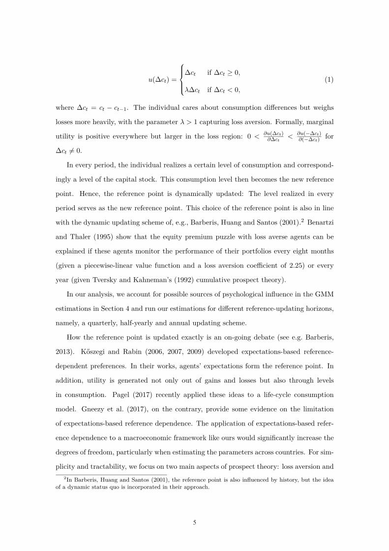
u(∆ct) =

∆ct if ∆ct ≥ 0,

λ∆ct if ∆ct < 0,

(1)

where ∆ct = ct − ct−1. The individual cares about consumption differences but weighs

losses more heavily, with the parameter λ > 1 capturing loss aversion. Formally, marginal

utility is positive everywhere but larger in the loss region: 0 < ∂u(∆ct)∂∆ct

< ∂u(−∆ct)∂(−∆ct) for

∆ct �= 0.

In every period, the individual realizes a certain level of consumption and correspond-

ingly a level of the capital stock. This consumption level then becomes the new reference

point. Hence, the reference point is dynamically updated: The level realized in every

period serves as the new reference point. This choice of the reference point is also in line

with the dynamic updating scheme of, e.g., Barberis, Huang and Santos (2001).2 Benartzi

and Thaler (1995) show that the equity premium puzzle with loss averse agents can be

explained if these agents monitor the performance of their portfolios every eight months

(given a piecewise-linear value function and a loss aversion coefficient of 2.25) or every

year (given Tversky and Kahneman’s (1992) cumulative prospect theory).

In our analysis, we account for possible sources of psychological influence in the GMM

estimations in Section 4 and run our estimations for different reference-updating horizons,

namely, a quarterly, half-yearly and annual updating scheme.

How the reference point is updated exactly is an on-going debate (see e.g. Barberis,

2013). Kőszegi and Rabin (2006, 2007, 2009) developed expectations-based reference-

dependent preferences. In their works, agents’ expectations form the reference point. In

addition, utility is generated not only out of gains and losses but also through levels

in consumption. Pagel (2017) recently applied these ideas to a life-cycle consumption

model. Gneezy et al. (2017), on the contrary, provide some evidence on the limitation

of expectations-based reference dependence. The application of expectations-based refer-

ence dependence to a macroeconomic framework like ours would significantly increase the

degrees of freedom, particularly when estimating the parameters across countries. For sim-

plicity and tractability, we focus on two main aspects of prospect theory: loss aversion and2In Barberis, Huang and Santos (2001), the reference point is also influenced by history, but the idea

of a dynamic status quo is incorporated in their approach.

5

6

thinking in differences. Foellmi, Rosenblatt-Wisch and Schenk-Hoppé (2011) show that

a utility function defined over these two aspects generates transitional dynamics different

from the standard Cass-Koopmans-Ramsey model. Namely, it leads to excess consump-

tion smoothing and can cause the economy to stay in a steady state of low consumption

and low capital.3 In addition, the length of our macroeconomic times series limits the

simultaneous estimation of several parameters. We will come back to this issue in Section

4.

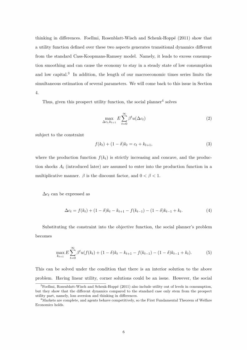
Thus, given this prospect utility function, the social planner4 solves

max∆ct,kt+1

E∞∑

t=0βtu(∆ct) (2)

subject to the constraint

f(kt) + (1 − δ)kt = ct + kt+1, (3)

where the production function f(kt) is strictly increasing and concave, and the produc-

tion shocks At (introduced later) are assumed to enter into the production function in a

multiplicative manner. β is the discount factor, and 0 < β < 1.

∆ct can be expressed as

∆ct = f(kt) + (1 − δ)kt − kt+1 − f(kt−1) − (1 − δ)kt−1 + kt. (4)

Substituting the constraint into the objective function, the social planner’s problem

becomes

maxkt+1

E∞∑

t=0βtu(f(kt) + (1 − δ)kt − kt+1 − f(kt−1) − (1 − δ)kt−1 + kt). (5)

This can be solved under the condition that there is an interior solution to the above

problem. Having linear utility, corner solutions could be an issue. However, the social3Foellmi, Rosenblatt-Wisch and Schenk-Hoppé (2011) also include utility out of levels in consumption,

but they show that the different dynamics compared to the standard case only stem from the prospectutility part, namely, loss aversion and thinking in differences.

4Markets are complete, and agents behave competitively, so the First Fundamental Theorem of WelfareEconomics holds.

6

7

planner approach unites maximization of households and firms. Even though utility is

linear with λ > 1, the production function is concave and, hence, the social planner

chooses an interior solution.

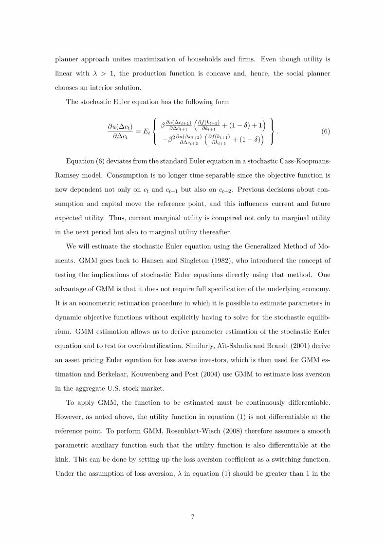
The stochastic Euler equation has the following form

∂u(∆ct)∂∆ct

= Et

β ∂u(∆ct+1)∂∆ct+1

(∂f(kt+1)

∂kt+1+ (1 − δ) + 1

)

−β2 ∂u(∆ct+2)∂∆ct+2

(∂f(kt+1)

∂kt+1+ (1 − δ)

)

. (6)

Equation (6) deviates from the standard Euler equation in a stochastic Cass-Koopmans-

Ramsey model. Consumption is no longer time-separable since the objective function is

now dependent not only on ct and ct+1 but also on ct+2. Previous decisions about con-

sumption and capital move the reference point, and this influences current and future

expected utility. Thus, current marginal utility is compared not only to marginal utility

in the next period but also to marginal utility thereafter.

We will estimate the stochastic Euler equation using the Generalized Method of Mo-

ments. GMM goes back to Hansen and Singleton (1982), who introduced the concept of

testing the implications of stochastic Euler equations directly using that method. One

advantage of GMM is that it does not require full specification of the underlying economy.

It is an econometric estimation procedure in which it is possible to estimate parameters in

dynamic objective functions without explicitly having to solve for the stochastic equilib-

rium. GMM estimation allows us to derive parameter estimation of the stochastic Euler

equation and to test for overidentification. Similarly, Aït-Sahalia and Brandt (2001) derive

an asset pricing Euler equation for loss averse investors, which is then used for GMM es-

timation and Berkelaar, Kouwenberg and Post (2004) use GMM to estimate loss aversion

in the aggregate U.S. stock market.

To apply GMM, the function to be estimated must be continuously differentiable.

However, as noted above, the utility function in equation (1) is not differentiable at the

reference point. To perform GMM, Rosenblatt-Wisch (2008) therefore assumes a smooth

parametric auxiliary function such that the utility function is also differentiable at the

kink. This can be done by setting up the loss aversion coefficient as a switching function.

Under the assumption of loss aversion, λ in equation (1) should be greater than 1 in the

7

8

loss area and exactly 1 in the gains area. Its value should switch as close as possible to

the reference point. Such a switching function f(·) for the loss aversion coefficient λ can

be represented by

f(∆c) = 1 + λ − 11 + eµ∆c

, (7)

where µ represents the speed of switching.

Figure 1: Switching Function

Note: µ responsible for the switching speed around the reference point with µ = 2 (bold line),µ = 4 (solid line) and µ = 6 (dashed line).

The higher µ is, the faster the switching around zero (see Figure 1). As required by the

assumption of loss aversion, the function f(∆c) approaches 1 for ∆c > 0 and λ for ∆c < 0.

Thus, expression (7) yields a smooth function to express the loss aversion coefficient λ in

the model. Inserting (7) for λ in the piecewise-linear utility function (1) and denoting

the parameterized marginal utility by u′(·) gives

u′(∆c) = 1 + λ − 11 + eµ(∆c) − (λ − 1) µ∆cte

µ∆ct

(1 + eµ∆ct)2 . (8)

8

9

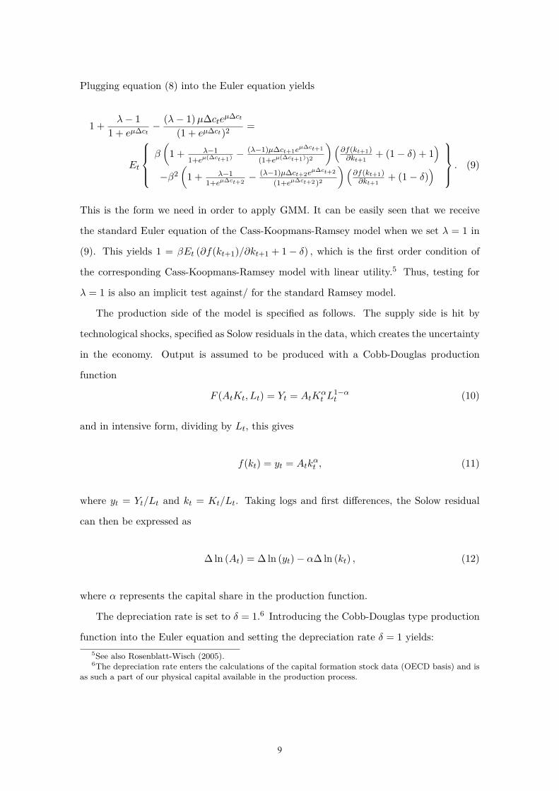
Plugging equation (8) into the Euler equation yields

1 + λ − 11 + eµ∆ct

− (λ − 1) µ∆cteµ∆ct

(1 + eµ∆ct)2 =

Et

β

(1 + λ−1

1+eµ(∆ct+1) − (λ−1)µ∆ct+1eµ∆ct+1

(1+eµ(∆ct+1))2

) (∂f(kt+1)

∂kt+1+ (1 − δ) + 1

)

−β2(

1 + λ−11+eµ∆ct+2 − (λ−1)µ∆ct+2eµ∆ct+2

(1+eµ∆ct+2 )2

) (∂f(kt+1)

∂kt+1+ (1 − δ)

)

. (9)

This is the form we need in order to apply GMM. It can be easily seen that we receive

the standard Euler equation of the Cass-Koopmans-Ramsey model when we set λ = 1 in

(9). This yields 1 = βEt (∂f(kt+1)/∂kt+1 + 1 − δ) , which is the first order condition of

the corresponding Cass-Koopmans-Ramsey model with linear utility.5 Thus, testing for

λ = 1 is also an implicit test against/ for the standard Ramsey model.

The production side of the model is specified as follows. The supply side is hit by

technological shocks, specified as Solow residuals in the data, which creates the uncertainty

in the economy. Output is assumed to be produced with a Cobb-Douglas production

function

F (AtKt, Lt) = Yt = AtKαt L1−α

t (10)

and in intensive form, dividing by Lt, this gives

f(kt) = yt = Atkαt , (11)

where yt = Yt/Lt and kt = Kt/Lt. Taking logs and first differences, the Solow residual

can then be expressed as

∆ ln (At) = ∆ ln (yt) − α∆ ln (kt) , (12)

where α represents the capital share in the production function.

The depreciation rate is set to δ = 1.6 Introducing the Cobb-Douglas type production

function into the Euler equation and setting the depreciation rate δ = 1 yields:5See also Rosenblatt-Wisch (2005).6The depreciation rate enters the calculations of the capital formation stock data (OECD basis) and is

as such a part of our physical capital available in the production process.

9

10

1 + λ − 11 + eµ∆ct

− (λ − 1) µ∆cteµ∆ct

(1 + eµ∆ct)2 =

Et

β

(1 + λ−1

1+eµ(∆ct+1) − (λ−1)µ∆ct+1eµ∆ct+1

(1+eµ(∆ct+1))2

) (αAt+1kα−1

t+1 + 1)

−β2(

1 + λ−11+eµ∆ct+2 − (λ−1)µ∆ct+2eµ∆ct+2

(1+eµ∆ct+2 )2

)αAt+1kα−1

t+1

. (13)

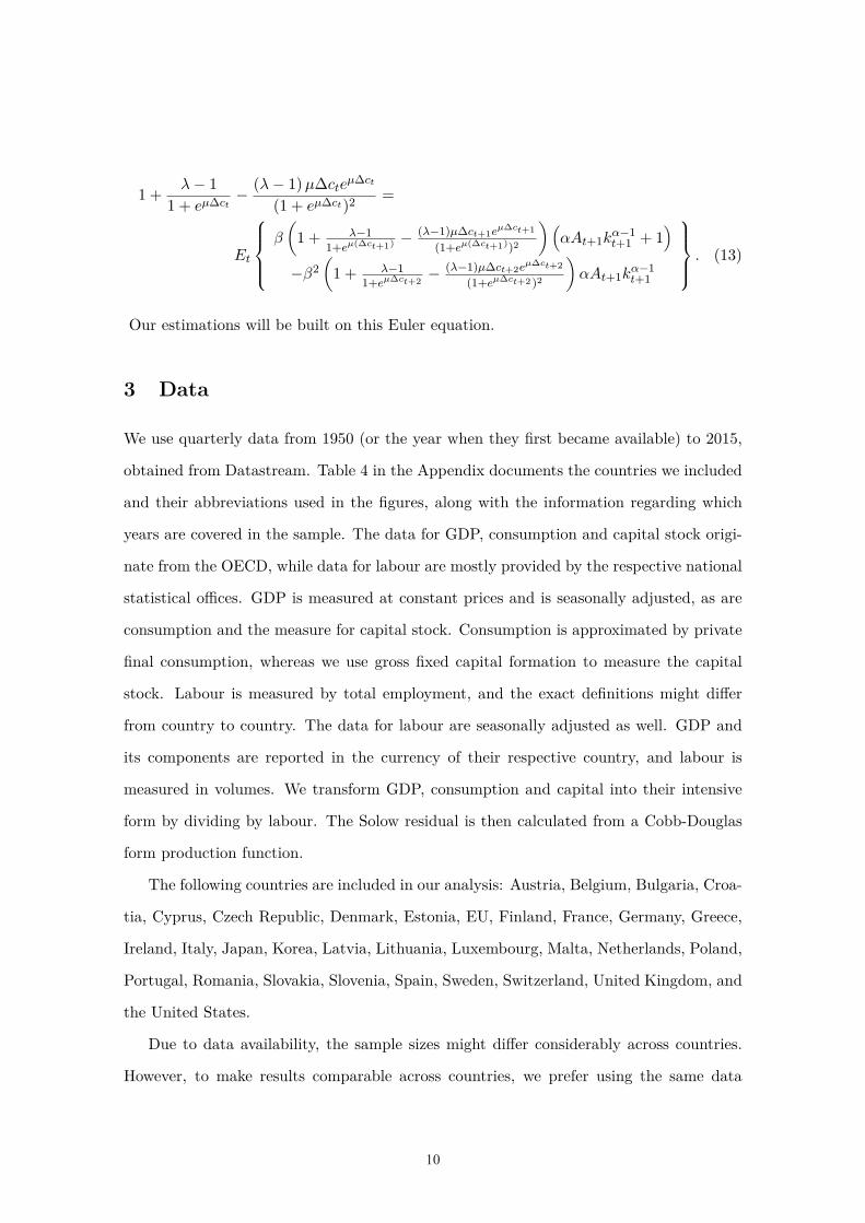
Our estimations will be built on this Euler equation.

3 Data

We use quarterly data from 1950 (or the year when they first became available) to 2015,

obtained from Datastream. Table 4 in the Appendix documents the countries we included

and their abbreviations used in the figures, along with the information regarding which

years are covered in the sample. The data for GDP, consumption and capital stock origi-

nate from the OECD, while data for labour are mostly provided by the respective national

statistical offices. GDP is measured at constant prices and is seasonally adjusted, as are

consumption and the measure for capital stock. Consumption is approximated by private

final consumption, whereas we use gross fixed capital formation to measure the capital

stock. Labour is measured by total employment, and the exact definitions might differ

from country to country. The data for labour are seasonally adjusted as well. GDP and

its components are reported in the currency of their respective country, and labour is

measured in volumes. We transform GDP, consumption and capital into their intensive

form by dividing by labour. The Solow residual is then calculated from a Cobb-Douglas

form production function.

The following countries are included in our analysis: Austria, Belgium, Bulgaria, Croa-

tia, Cyprus, Czech Republic, Denmark, Estonia, EU, Finland, France, Germany, Greece,

Ireland, Italy, Japan, Korea, Latvia, Lithuania, Luxembourg, Malta, Netherlands, Poland,

Portugal, Romania, Slovakia, Slovenia, Spain, Sweden, Switzerland, United Kingdom, and

the United States.

Due to data availability, the sample sizes might differ considerably across countries.

However, to make results comparable across countries, we prefer using the same data

10

11

source, if possible, for all countries, which comes at the price of having fewer data points

for some countries.

4 Loss Aversion Across Countries

4.1 Estimation: Loss Aversion Coefficients Across Countries

We estimate equation (13) using GMM. An advantage of GMM estimation is that we do

not have to know, or to specify, the full economic setting of the underlying economy.

It would be desirable to jointly estimate loss aversion λ, the capital share α and the

discount factor β in equation (13), since these parameters might vary across countries.

However, the data at hand are not sufficient to estimate these three parameters jointly.

GMM does no longer converge in most specifications when estimating more than one

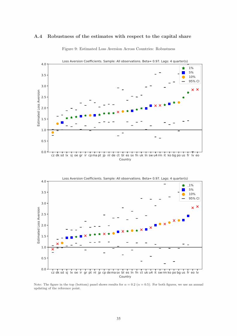
parameter. We set the capital share α equal to 0.33 and µ equal to 0.1, for computational

efficiency. α equal to 0.33 is a standard value.7 As a robustness check, we also perform

our calculations for α equal to 0.2 and 0.5. The results remain robust (see Figure 9 in the

Appendix).

For the discount factor β, we use four different values: 0.90, 0.95, 0.97 and 0.99.

We hold the discount factor constant across countries, which is the common approach in

current DSGE modelling across countries (see e.g. Justiniano and Preston, 2009).8

We only report results if we have at least 15 observations, which is true for all coun-

tries if we use the full sample. As a special case, we are also investigating whether the

loss aversion coefficients across countries have converged over time, with a particular in-

terest in the Euro Area countries after the introduction of the Euro as a single currency.

We, therefore, also estimate equation (13) for two sub-samples (pre-2000 and post-2000).

However, for the pre-2000 sub-sample, we do not have enough observations for Poland,

Czech Republic, Romania, Bulgaria, Malta, Croatia, Cyprus, Lithuania and Greece.

For the specifications of the estimation, we follow the strategy used in Rosenblatt-7 See, for example, Abel and Bernanke (2001) or Hall and Taylor (1997).8Our data only covers well-developed OECD countries with well-integrated financial markets. The

discount factor in stochastic models represents a long-run average real return on risky and riskless assets.One could think of a broad portfolio, or from a finance point of view of the market portfolio. With globalfinancial integration this market portfolio can be assessed by each country and should therefore be similaracross countries.

11

12

Wisch (2008). In the baseline specification, we estimate equation (13) without additional

moment conditions. As a robustness check, we also introduce additional moment condi-

tions in which we use lagged values as instruments: Assuming individuals form expec-

tations rationally, they use information from period t to form expectations about period

t + 1 but no information from earlier periods. Hence, lagged variables are not correlated

with the error terms. In total, we consider seven different specifications concerning the

moment conditions. As mentioned, the baseline version is the one without instruments.

The other six specifications include lagged values of consumption differences, capital and

combinations of it, to formulate additional moment restrictions.

In macroeconomic time series, it is common for the error terms to be correlated over

time. Therefore, to allow for heteroscedasticity and autocorrelation in the residuals, we

use a heteroscedasticity-and autocorrelation-consistent (HAC) weighing matrix (in case

we use instrumental variables) as well as HAC standard errors, using the Bartlett kernel

with 4 lags. We use an iterative GMM estimator since it might be more efficient in

finite samples (Hall, 2005, p. 88–94), and, as is often the case with macroeconomic time

series, our empirical investigation is performed in small samples, which makes this strategy

particularly appealing (Hansen, Heaton and Yaron, 1996).

Furthermore, we verify that all input series are stationary, since GMM relies on the

stationarity of the components. The null hypothesis of a unit root (tested by the aug-

mented Dickey-Fuller test) can be rejected for all input series for all countries considered.

The consumption series are first-difference stationary. We define the Solow residual in

terms of growth rates for technological progress together with the growth rate of capital

productivity. Using the exponential of the Solow residual generates a stationary time

series for the production part of our Euler equation.

4.2 Results: Loss Aversion Coefficients Across Countries

First, we confirm the results found in Rosenblatt-Wisch (2008) for a large set of OECD

countries. In general, it seems to hold true that we can track loss aversion in an aggregate

time series for different countries and across various specifications of the estimated model.

Second, and as expected, we find that larger values of β lead to lower estimates of the loss

aversion parameter. As documented in Rosenblatt-Wisch (2008), a higher value for β as

12

13

well as a higher degree of loss aversion imply that the individual is hurt more by future

losses. Hence, β and λ work in the same direction, which implies that when fixing a data

point, the higher β is, the lower λ has to be and vice versa. This result is confirmed in

the data, across specifications as well as across countries.

Table 1 presents the results in detail for one country, namely, the United States. We

estimate various specifications with and without instrumental variables. To keep the

exposition tractable, some further results are included in the Appendix. The estimates

are very similar to those found in Rosenblatt-Wisch (2008). Overall, the results reveal

highly significant estimates of the loss aversion coefficient.

Table 1: Results for the US Without Additional Moment RestrictionsReference point adj. 1 quarter 2 quarters 4 quarters

β = 0.90λ 1.949*** 2.516*** 4.441***

Stv Dev 0.129 0.306 1.146p value 0.000 0.000 0.003

β = 0.95λ 1.589*** 1.913*** 3.011***

Stv Dev 0.096 0.206 0.739p value 0.000 0.000 0.007

β = 0.97λ 1.428*** 1.652*** 2.388**

Stv Dev 0.083 0.166 0.553p value 0.000 0.000 0.012

β = 0.99λ 0.820*** 1.339*** 1.670*

Stv Dev 0.043 0.124 0.347p value 0.000 0.006 0.054

Nobs 243 243 243Note: *,**,*** denote statistical significance at the 1%, 5% and 10%level.

Tables 6 and 7 in the Appendix show the results for the United States when using

lagged consumption (Table 6) and lagged capital stock (Table 7) as an instrument. The

results documented in Table 1 can be confirmed. For the specification with β = 0.97, the

loss aversion coefficient is estimated to be 1.3 for the semi-annual updating scheme and 2.2

for the annual update scheme, when using lagged consumption as the instrument. These

numbers change slightly to 1.6 and 2.4, respectively, when using lagged capital stock as

the instrument. All estimates are highly significant. These estimates are close to Tversky

and Kahneman’s experimentally supported value of 2.25 for the loss aversion coefficient.

13

14

These findings carry over to a broad set of OECD countries: Basically, all estimates

are above 1, indicating loss aversion and are statistically significant. Figure 2 summarizes

the results for the estimates resulting from the specifications without instruments for a

discount factor of β = 0.97 and from semi-annual as well as annual reference point updating

(for tractability we will use these two specifications as our baseline results for the rest of

the paper). We find loss aversion in all countries. The results are somewhat stronger

for the semi-annual reference point updating scheme compared to the annual updating

scheme.

Furthermore, not only do we find loss aversion in all countries, but we also find cross-

country differences in the degree of loss aversion. This holds particularly true for larger

updating horizons. Even though the order of the countries when ranked according to their

estimated loss aversion coefficient is subject to changes across different specifications, we

observe that some country groups are often clustered together at similar loss aversion

coefficients.

14

15

Figure 2: Estimated Loss Aversion Across Countries

Note: Figure in the top (bottom) panel shows results for semi-annual (annual) reference point updating.

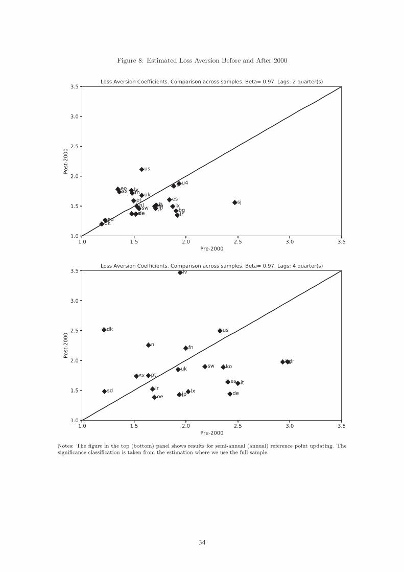
Finally, we test for convergence of loss aversion across countries, comparing the pre-

2000 and post-2000 samples. We do not find robust evidence for differences in loss aversion

15

16

when comparing the pre-2000 sample with the post-2000 sample. Our data do not suggest

that we see cross-country convergence in loss aversion. Figure 8 in the Appendix shows

the estimated loss aversion coefficients for the pre-2000 and the post-2000 sample, using

β = 0.97 and a semi-annual as well as an annual reference-point updating scheme. Visual

inspection does not suggest that the variation in the estimates along the post-2000 axis is

smaller than along the pre-2000 axis. To underpin this finding, we report the results from a

variance comparison test in Table 8 in the Appendix. There, we test whether the standard

deviations of the cross-country estimates are significantly different for the two samples.

As the last column reveals, we can reject the null-hypothesis that the standard deviations

are the same for only three specifications with an updating horizon of one quarter—the

specifications in which the standard deviations across countries are very small. For all

other specifications, we do not find any evidence that loss aversion has converged.

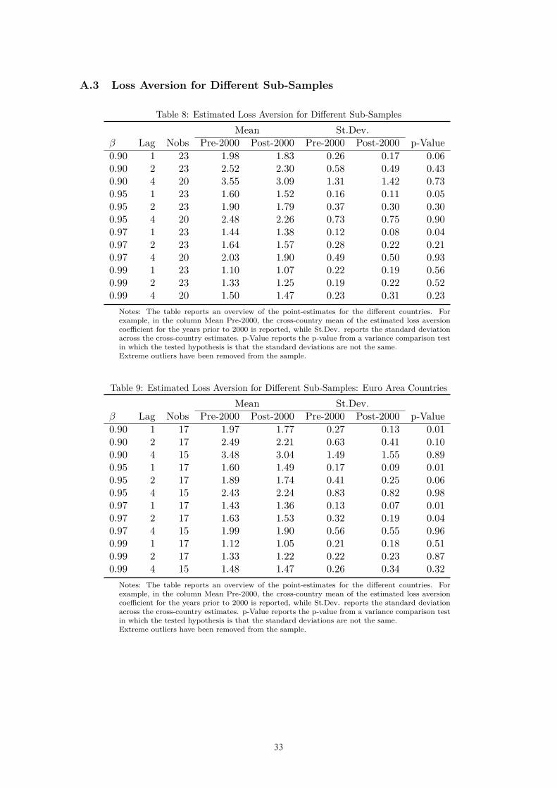
Conceivably, institutional settings and loss aversion are closely inter-linked. In Table

9 in the Appendix, we repeat the variance comparison test for the sample of countries

within the Euro Area only, accounting for the fact that Euro Area countries’ preferences

could have become more identical after the year 2000, i.e., after having formed a monetary

union, or differently said, after having changed the institutional settings. Table 9, however,

shows that convergence in preferences has not taken place to date. We cannot reject the

null-hypothesis that the standard deviations of the estimates in the two sub-samples are

the same for most specifications.

To sum up, the results found in Rosenblatt-Wisch (2008) for the United States basically

carry over to other countries: We consistently find loss aversion coefficients that exceed

one (indicating individuals are loss averse), and interestingly, we also find pronounced

variation in the size of the loss aversion coefficients across countries.

Can these differences in loss aversion at the aggregate level across countries be ex-

plained by micro evidence? We investigate this question in the next subsection. Specif-

ically, we check how our estimated loss aversion coefficients are related to the cultural

dimensions reported by Hofstede, Hofstede and Minkov (2010), as well as how they relate

to some key questions from the World Values Survey (WVS).

16

17

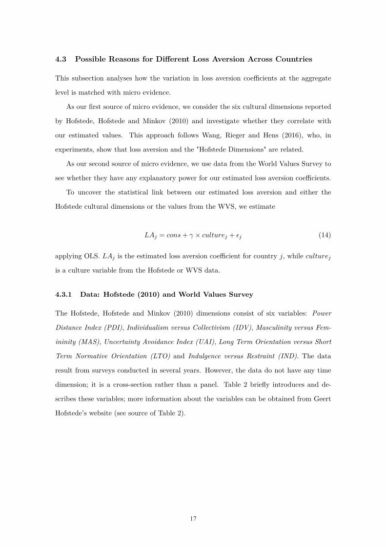
4.3 Possible Reasons for Different Loss Aversion Across Countries

This subsection analyses how the variation in loss aversion coefficients at the aggregate

level is matched with micro evidence.

As our first source of micro evidence, we consider the six cultural dimensions reported

by Hofstede, Hofstede and Minkov (2010) and investigate whether they correlate with

our estimated values. This approach follows Wang, Rieger and Hens (2016), who, in

experiments, show that loss aversion and the "Hofstede Dimensions" are related.

As our second source of micro evidence, we use data from the World Values Survey to

see whether they have any explanatory power for our estimated loss aversion coefficients.

To uncover the statistical link between our estimated loss aversion and either the

Hofstede cultural dimensions or the values from the WVS, we estimate

LAj = cons + γ × culturej + εj (14)

applying OLS. LAj is the estimated loss aversion coefficient for country j, while culturej

is a culture variable from the Hofstede or WVS data.

4.3.1 Data: Hofstede (2010) and World Values Survey

The Hofstede, Hofstede and Minkov (2010) dimensions consist of six variables: Power

Distance Index (PDI), Individualism versus Collectivism (IDV), Masculinity versus Fem-

ininity (MAS), Uncertainty Avoidance Index (UAI), Long Term Orientation versus Short

Term Normative Orientation (LTO) and Indulgence versus Restraint (IND). The data

result from surveys conducted in several years. However, the data do not have any time

dimension; it is a cross-section rather than a panel. Table 2 briefly introduces and de-

scribes these variables; more information about the variables can be obtained from Geert

Hofstede’s website (see source of Table 2).

17

18

Table 2: Summary Description of the Hofstede VariablesVariable Description

Power Distance Index Measures the degree to which less powerful individuals accept that power isdistributed unequally. People living in societies with a high Power Distanceaccept a hierarchical order in which everyone has his or her place.

Individualism vs. Collectivism Measures the degree of individualism, i.e., to what degree members of a societyare only expected to take care of themselves and their family. People livingin societies with a high degree of individualism define their self-image as "I",whereas people in collectivist societies define themselves as "We".

Masculinity vs. Femininity Measures the importance of achievement and material success in society. Mas-culine societies tend to be competitive, while feminine societies are moreconsensus-oriented.

Uncertainty Avoidance Index Measures the degree to which the members of society feel uncomfortable withuncertainty or ambiguity. Societies with a higher score want to try to controlthe future, while societies with a low score just let the future happen.

Long Term Orientation Measures how societies value the future in terms of the present and past. So-cieties that score low view social change with suspicion, while societies with ahigh score encourage thrift and education to prepare for the future.

Indulgence vs. Restraint Measures to what degree human drives are regulated by social norms. Indulgentsocieties allow free gratification of drives related to enjoying life and having fun.In restraint societies, gratification is regulated to a stronger degree by strictsocial norms.

Source: Hofstede, Hofstede and Minkov (2010); Geert Hofstede’s website: https://geert-hofstede.com/national-culture.html. More detailed information about the six variables, as well as the measurement ofthe variables, can be found there.

Descriptive statistics for the Hofstede variables used here are provided in part I of

Table 5 in the Appendix. Wang, Rieger and Hens (2016) use only the first four of these

dimensions to establish a link between them and loss aversion, mostly on the individual

level. They find that individuals with a higher value for PDI and IDV are more loss averse

and that individuals living in countries with a higher value for MAS are more loss averse.

However, they do not include LTO and IND in their paper.

Our second source, the World Values Survey9, includes more than 800 individual ques-

tions. Hence, we are required to select some "key" variables that we consider to have an

impact on our estimate of loss aversion. Table 3 lists our selected variables, while we

provide descriptive statistics in part II of Table 5 in the Appendix. Variable is how we

name them, and Code is the code for the question asked in the WVS data. Description

is a short description of the content of the variable. The variables are selected partly

because we think they are important for economic outcomes and partly because they were

used in earlier economic studies. For example, the question we selected to measure time

preferences, A038, was used in Galor and Oezak (2016) to proxy for long-term orientation

or patience.9The WVS data can be obtained from http://www.worldvaluessurvey.org/wvs.jsp

18

19

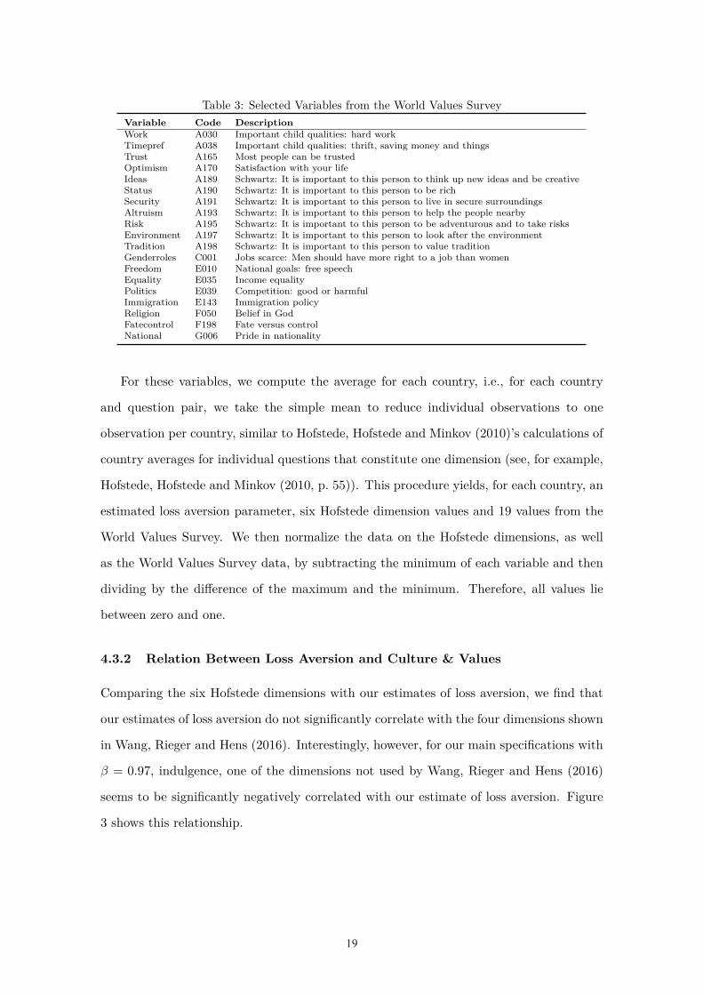
Table 3: Selected Variables from the World Values SurveyVariable Code DescriptionWork A030 Important child qualities: hard workTimepref A038 Important child qualities: thrift, saving money and thingsTrust A165 Most people can be trustedOptimism A170 Satisfaction with your lifeIdeas A189 Schwartz: It is important to this person to think up new ideas and be creativeStatus A190 Schwartz: It is important to this person to be richSecurity A191 Schwartz: It is important to this person to live in secure surroundingsAltruism A193 Schwartz: It is important to this person to help the people nearbyRisk A195 Schwartz: It is important to this person to be adventurous and to take risksEnvironment A197 Schwartz: It is important to this person to look after the environmentTradition A198 Schwartz: It is important to this person to value traditionGenderroles C001 Jobs scarce: Men should have more right to a job than womenFreedom E010 National goals: free speechEquality E035 Income equalityPolitics E039 Competition: good or harmfulImmigration E143 Immigration policyReligion F050 Belief in GodFatecontrol F198 Fate versus controlNational G006 Pride in nationality

For these variables, we compute the average for each country, i.e., for each country

and question pair, we take the simple mean to reduce individual observations to one

observation per country, similar to Hofstede, Hofstede and Minkov (2010)’s calculations of

country averages for individual questions that constitute one dimension (see, for example,

Hofstede, Hofstede and Minkov (2010, p. 55)). This procedure yields, for each country, an

estimated loss aversion parameter, six Hofstede dimension values and 19 values from the

World Values Survey. We then normalize the data on the Hofstede dimensions, as well

as the World Values Survey data, by subtracting the minimum of each variable and then

dividing by the difference of the maximum and the minimum. Therefore, all values lie

between zero and one.

4.3.2 Relation Between Loss Aversion and Culture & Values

Comparing the six Hofstede dimensions with our estimates of loss aversion, we find that

our estimates of loss aversion do not significantly correlate with the four dimensions shown

in Wang, Rieger and Hens (2016). Interestingly, however, for our main specifications with

β = 0.97, indulgence, one of the dimensions not used by Wang, Rieger and Hens (2016)

seems to be significantly negatively correlated with our estimate of loss aversion. Figure

3 shows this relationship.

19

20

Figure 3: Estimated Loss Aversion and Indulgence

lv

bl

ln

eorm

sxpo

ko

cz

it

pt

ct

dejp

es

fr

sjgr

lxbgfn

oeirswmanl

usuk

dksd

1.2

1.4

1.6

1.8

22.

2Es

timat

ed L

oss

Aver

sion

0 .2 .4 .6 .8 1

IndulgenceRegression Coefficient: -.55 ----- p-value: 0 ----- nObs: 30

lveo

blln

rm

sx

kopo

cz

it

ptct

dejpes

sj

fr

grlx

fn

bg

oeirma

sw

nl

us

uk

dk sd

11.

52

2.5

3Es

timat

ed L

oss

Aver

sion

0 .2 .4 .6 .8 1

IndulgenceRegression Coefficient: -.84 ----- p-value: .04 ----- nObs: 30

Note: Figure in the left (right) panel shows results for semi-annual (annual) reference point updating.

The left panel in Figure 3 uses the estimated loss aversion coefficient with a semi-annual

updating scheme, whereas the right panel uses the results from the specification with an

annual scheme. Indulgence measures how individuals are able to control their impulses.

A lower score implies that individuals are more restrained (i.e., more able to control their

impulses and desires), which is related to a higher degree of loss aversion. Furthermore,

we find that long-term orientation, the last remaining dimension and not shown in Wang,

Rieger and Hens (2016), is positively correlated with loss aversion. However, the link is not

statistically significant. The results for indulgence and long-term orientation seem to be

in line with the status quo bias that loss aversion induces (see Samuelson and Zeckhauser,

1988). The more loss averse an agent is, the higher is his status quo bias. The status

quo bias can be interpreted as a long-term orientation and as not being tempted by short-

sighted impulses and desires.

For the selected indicators from the World Values Survey, a similar picture emerges:

Most of the variables do not seem to be statistically significantly correlated with our

estimates of loss aversion. One indicator that seems to have some explanatory power for

loss aversion is optimism: Pessimistic people show higher loss aversion. This relationship

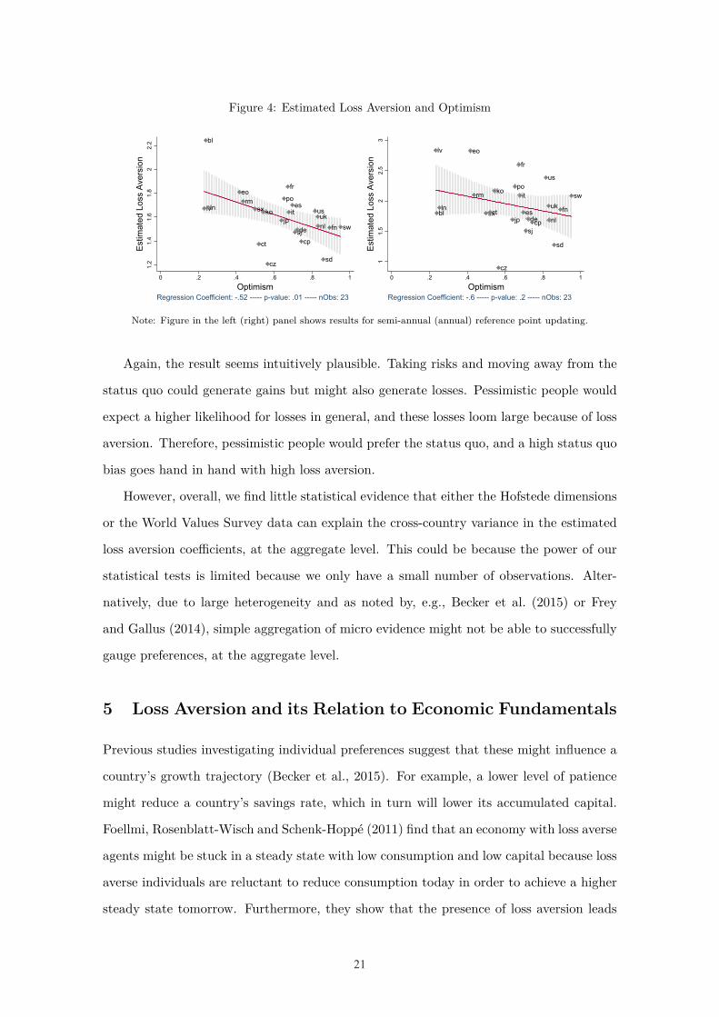
is shown in Figure 4.

20

21

Figure 4: Estimated Loss Aversion and Optimism

lv

bl

ln

eorm

sx

ct

ko

cz

jp

po

fr

ites

sjde

cp

usuknl

sd

fn sw

1.2

1.4

1.6

1.8

22.

2Es

timat

ed L

oss

Aver

sion

0 .2 .4 .6 .8 1

OptimismRegression Coefficient: -.52 ----- p-value: .01 ----- nObs: 23

lv

blln

eo

rm

sxct

ko

cz

jp

po

fr

it

es

sj

decp

us

uk

nl

sd

fn

sw

11.

52

2.5

3Es

timat

ed L

oss

Aver

sion

0 .2 .4 .6 .8 1

OptimismRegression Coefficient: -.6 ----- p-value: .2 ----- nObs: 23


Again, the result seems intuitively plausible. Taking risks and moving away from the

status quo could generate gains but might also generate losses. Pessimistic people would

expect a higher likelihood for losses in general, and these losses loom large because of loss

aversion. Therefore, pessimistic people would prefer the status quo, and a high status quo

bias goes hand in hand with high loss aversion.

However, overall, we find little statistical evidence that either the Hofstede dimensions

or the World Values Survey data can explain the cross-country variance in the estimated

loss aversion coefficients, at the aggregate level. This could be because the power of our

statistical tests is limited because we only have a small number of observations. Alter-

natively, due to large heterogeneity and as noted by, e.g., Becker et al. (2015) or Frey

and Gallus (2014), simple aggregation of micro evidence might not be able to successfully

gauge preferences, at the aggregate level.

5 Loss Aversion and its Relation to Economic Fundamentals

Previous studies investigating individual preferences suggest that these might influence a

country’s growth trajectory (Becker et al., 2015). For example, a lower level of patience

might reduce a country’s savings rate, which in turn will lower its accumulated capital.

Foellmi, Rosenblatt-Wisch and Schenk-Hoppé (2011) find that an economy with loss averse

agents might be stuck in a steady state with low consumption and low capital because loss

averse individuals are reluctant to reduce consumption today in order to achieve a higher

steady state tomorrow. Furthermore, they show that the presence of loss aversion leads

21

22

to stronger consumption smoothing.

Hence, we investigate whether our estimated loss aversion coefficients (again with the

specification of β = 0.97) are correlated with a series of economic fundamentals series, such

as GDP per capita, consumption, savings rates, inflation, investment shares, monetary

aggregates and long-term interest rates. Furthermore, we also look at correlations between

unemployment benefits and financial openness with loss aversion. Since the estimated loss

aversion coefficients are constant over time, we select the economic fundamentals from the

year 2010 as well as the year 2000 to exclude potential effects of the crisis. Furthermore, we

look at averages over the years as well as fluctuations of these variables over the years, in

order to capture long-term trends as well as business cycle fluctuations of these variables.

As we only have 32 observations, we look at bivariate relationships. Obviously, many

other factors affect a country’s growth trajectory or other economic fundamentals, while

driving loss aversion at the same time. However, due to data limitations, this section

focuses on correlations only. By doing so, we shed some light on potential links between

loss aversion and economic fundamentals, without claiming any causal relationship.

5.1 Data

We retrieve data for the economic fundamentals from standard macroeconomic data

sources. For the long-term interest rates, we use 10-year government bond yields from

the OECD database. For the monetary aggregates, we use the broad money (M3) index

taken from the OECD database as well. From the same database, we include data on

the replacement ratio (for a single individual having worked full time) and an index of

financial services restrictions to proxy financial openness. Real GDP and consumption are

taken from the Penn World Tables (Version 8.1) and adjusted to per-capita terms, using

population data from the same database.10 Additionally, from the Penn World Tables,

we take shares of household consumption and government consumption. Finally, we use

annual inflation, broad money (M3) as a % of GDP and savings rates reported in the

World Development Indicators (WDI), provided by the World Bank. Summary statistics10We use GDP and consumption data from the Penn World Tables here as a standard source for macroe-

conomic data. Note, that they are only available at annual frequency, which is sufficient for the exercise inthis section. For the estimations of the loss aversion parameters, we used quarterly data from the OECDdatabase.

22

23

for these variables can be found in part III of Table 5 in the Appendix. For the loss

aversion coefficients, we use our point estimates, using the baseline specifications without

additional moment restriction, a discount factor of β = 0.97 and semi-annual and annual

reference point adjustments.

5.2 Results

We investigate the statistical link between the economic fundamentals introduced above

and the estimated loss aversion, applying OLS. Hence,

Yj = cons + θ × LAj + υj , (15)

where Yj is any economic fundamental in country j, either at a given point in time (i.e.,

in either the year 2000 or 2010), or the average over time, or (in the case of consumption

smoothing) the standard deviation over time. LAj again is the estimated loss aversion in

country j.

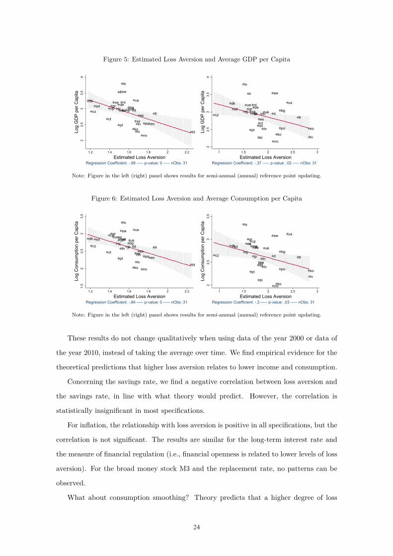
Among the economic fundamentals investigated, we find a consistent and significant

effect for GDP per capita and consumption: Less loss aversion is significantly correlated

with higher consumption levels as well as GDP per capita. Figures 5 and 6 summarize

this result. Here, we use the average of GDP per capita over the same sample for which

we have data to estimate the loss aversion coefficient. For Switzerland, for example, we

have data from 1970 onward to estimate the Euler equation (see Table 4 in the Appendix),

and, hence, we calculate, in this case, the average GDP per capita since 1970. Again, the

left panel uses semi-annual reference point updating, whereas the right panel uses annual

updating.

23

24

Figure 5: Estimated Loss Aversion and Average GDP per Capita

dk

czsd

ct

cpgroe

sjde

pt

ir

mafn

sw

nl

lx

jpbgukit

ko

us

sx

lv

ln

es

rm

po eo

fr

bl

22.

53

3.5

4Lo

g G

DP

per C

apita

1.2 1.4 1.6 1.8 2 2.2

Estimated Loss AversionRegression Coefficient: -.99 ----- p-value: 0 ----- nObs: 31

cz

dksd

lx

sj

oegr

ir

pt

cpma

nl

jpde

sx

bl

esct

fn

ln

uk

sw

it

rm

kopo

bg

us

fr

eo

lv

22.

53

3.5

4Lo

g G

DP

per C

apita

1 1.5 2 2.5 3

Estimated Loss AversionRegression Coefficient: -.37 ----- p-value: .02 ----- nObs: 31


Figure 6: Estimated Loss Aversion and Average Consumption per Capita

dk

cz

sd

ct

cpgroe

sjdeir

pt

ma

fn

sw

nl

lx

jpbguk

it

ko

us

sx

lv

lnes

rm

po eo

fr

bl

1.5

22.

53

3.5

Log

Con

sum

ptio

n pe

r Cap

ita

1.2 1.4 1.6 1.8 2 2.2

Estimated Loss AversionRegression Coefficient: -.84 ----- p-value: 0 ----- nObs: 31

cz

dksd

lx

sj

oegrir

pt

cpmanl

jp

de

sx

bl

esctfn

ln

uk

sw

it

rmko

bg

po

us

fr

eolv

22.

53

3.5

Log

Con

sum

ptio

n pe

r Cap

ita

1 1.5 2 2.5 3



These results do not change qualitatively when using data of the year 2000 or data of

the year 2010, instead of taking the average over time. We find empirical evidence for the

theoretical predictions that higher loss aversion relates to lower income and consumption.

Concerning the savings rate, we find a negative correlation between loss aversion and

the savings rate, in line with what theory would predict. However, the correlation is

statistically insignificant in most specifications.

For inflation, the relationship with loss aversion is positive in all specifications, but the

correlation is not significant. The results are similar for the long-term interest rate and

the measure of financial regulation (i.e., financial openness is related to lower levels of loss

aversion). For the broad money stock M3 and the replacement rate, no patterns can be

observed.

What about consumption smoothing? Theory predicts that a higher degree of loss

24

25

aversion goes hand in hand with more consumption smoothing. Therefore, we calculate

the standard deviation of the share of household consumption in output over the years for

each country in our sample. This gives a simple measure of the fluctuations in consumption

shares. We expect a negative correlation between this measure and loss aversion.11 Figure

7 illustrates this finding.

Figure 7: Estimated Loss Aversion and Fluctuations in Consumption

dk

cz

sd

ct

cp

groe

sjde

ir

pt

fnswnl

lx

jpbgukit

ko

ussx

lvlnesrm

po eofr

bl

0.0

5.1

.15

.2St

.Dev

. of C

onsu

mpt

ion

Shar

e

1.2 1.4 1.6 1.8 2 2.2


cz

dksd

lx

sjoegr

ir

pt

cp

nljpde sx

bles

ctfn

ln

ukswit

rm

ko

bgpo us

freo

lv0

.05

.1.1

5.2

St.D

ev. o

f Con

sum

ptio

n Sh

are

1 1.5 2 2.5 3



Looking at the raw correlation, the two measures seem to be negatively correlated,

but the relationship is not significant. However, it is likely that a high level of GDP is

both negatively correlated with loss aversion and negatively correlated with fluctuations

in consumption. Indeed, if we include average GDP over the years in our estimation

(by adding average GDP as an additional regressor to equation (15)), the link between

the standard deviation of consumption over time and estimated loss aversion becomes

statistically stronger. Note that the statistical link found is stronger than suggested by

Figure 7 because we need to control for GDP. As indicated at the bottom of the figures,

using semi-annual reference point updating, the p-value is 0.11, whereas with annual

reference point updating, it is 0.08. Hence, we find some indicative evidence for a link

between loss aversion and consumption smoothing, as theory would suggest.11We exclude Malta here, since its standard deviation of consumption is very large and therefore this

data point is a huge outlier.

25

26

6 Conclusions

Preferences of agents matter when thinking about macroeconomic modelling and economic

developments. In this paper, we find evidence for loss aversion for a broad set of OECD

countries, at the aggregate level. The average degree of loss aversion clearly differs across

these countries. To understand these differences, we explore the correlation between loss

aversion and macroeconomic fundamentals. We find that GDP per capita and consumption

levels are significantly and negatively related to our estimates of loss aversion, in line

with what theory would predict. Furthermore, we find a higher degree of consumption

smoothing in countries with a higher loss aversion.

To gain more insights on the link between institutions and preferences, we also checked

whether loss aversion has converged over time, and, in particular, among Euro Area coun-

tries after the introduction of the Euro as the single currency. This seems not to have

taken place to date.

To understand the underlying reasons of how reference points are formed, it would

be interesting to incorporate expectations-based reference dependence. However, such an

approach would increase the degrees of freedom substantially, in particular, when esti-

mating the parameters across countries. The data at hand is not sufficient to perform

this exercise. However, as time goes by, the length of the macro time series extends. We,

therefore, leave this exercise to future research.

26

27

ReferencesAbdellaoui, Mohammed, Han Bleichrodt, and Corina Paraschiv Paraschiv.

2007. “Loss Aversion under Prospect Theory: A Parameter-Free Measurement.” Man-agement Science, 53(10): 1659–1674.

Abel, Andrew B., and Ben S. Bernanke. 2001. Macroeconomics. Addison WesleyLongman, Boston.

Aït-Sahalia, Yacine, and Michael W. Brandt. 2001. “Variable selection for portfoliochoice.” Journal of Finance, 56: 1297–1351.

Barberis, Nicholas C. 2013. “Thirty Years of Prospect Theory in Economics: A Reviewand Assessment.” Journal of Economic Perspectives, 27(1): 173–196.

Barberis, Nicholas, Ming Huang, and Tano Santos. 2001. “Prospect Theory andAsset Prices.” The Quarterly Journal of Economics, 116(1): 1–53.

Becker, Anke, Thomas J. Dohmen, Benjamin Enke, Armin Falk, David Huff-man, and Uwe Sunde. 2015. “The Nature and Predictive Power of Preferences: GlobalEvidence.” CEPR Discussion Papers.

Benartzi, Shlomo, and Richard H. Thaler. 1995. “Myopic Loss Aversion and theEquity Premium Puzzle.” The Quarterly Journal of Economics, 110(1): 73–92.

Berkelaar, Arjan B., Roy Kouwenberg, and Thierry Post. 2004. “Optimal portfoliochoice under loss aversion.” Review of Economics and Statistics, 86: 973–987.

Brooks, Peter, and Horst Zank. 2005. “Loss averse behavior.” Journal of Risk andUncertainty, 31: 301–325.

Chen, M. Keith, Venkat Lakshminarayanan, and Laurie R. Santos. 2006. “HowBasic Are Behavioral Biases? Evidence from Capuchin Monkey Trading Behavior.”Journal of Political Economy, 114(3): 517–537.

Foellmi, Reto, Rina Rosenblatt-Wisch, and Klaus Reiner Schenk-Hoppé. 2011.“Consumption paths under prospect utility in an optimal growth model.” Journal ofEconomic Dynamics and Control, 35(3): 273–281.

Frey, Bruno S., and Jana Gallus. 2014. “Aggregate Effects of Behavioral Anomalies:A New Research Area.” Economics, Psychology and Choice Theory, 8(18).

Galor, Oded, and Oemer Oezak. 2016. “The Agricultural Origins of Time Preference.”American Economic Review, 106(10): 3064–3103.

Gneezy, Uri, Lorenz Goette, Charles Sprenger, and Florian Zimmermann.2017. “The limits of Expectations-based reference dependence.” Journal of the EuropeanEconomic Association, forthcoming.

Hall, Alastair R. 2005. Generalized method of moments. Oxford University Press Oxford.

Hall, Robert E., and John B. Taylor. 1997. Macroeconomics. Norton, New York.

Hansen, Lars Peter, and Kenneth J. Singleton. 1982. “Generalized Instrumen-tal Variables Estimation of Nonlinear Rational Expectations Models.” Econometrica,50(5): 1269–1286.

27

28

Hansen, Lars Peter, John Heaton, and Amir Yaron. 1996. “Finite-Sample Proper-ties of Some Alternative GMM Estimators.” Journal of Business & Economic Statistics,14(3): 262–280.

Herrmann, Benedikt, Christian Thöni, and Simon Gächter. 2008. “AntisocialPunishment Across Societies.” Science, 319(5868): 1362–1367.

Hofstede, Geert, Gert Jan Hofstede, and Michael Minkov. 2010. Cultures andOrganizations - Software of the Mind. McGraw-Hill Education Ltd.

Justiniano, Alejandro, and Bruce Preston. 2009. “Monetary Policy and Uncertaintyin an Empirical Small Open Economy Model.” Federal Reserve Bank of Chicago, Work-ing Paper 2009-21.

Kahneman, Daniel, and Amos Tversky. 1979. “Prospect Theory: An Analysis ofDecision under Risk.” Econometrica, 47(2): 263–291.

Kahneman, Daniel, Jack L. Knetsch, and Richard H. Thaler. 1990. “Experimentaltests of the endowment effect and the coase theorem.” Journal of Political Economy,98: 1325–1348.

Kőszegi, Botond, and Matthew Rabin. 2006. “A model of reference-dependent pref-erences.” Quarterly Journal of Economics, 121: 1133–1165.

Kőszegi, Botond, and Matthew Rabin. 2007. “Reference-dependent risk attitudes.”American Economic Review, 97: 1047–1073.

Kőszegi, Botond, and Matthew Rabin. 2009. “Reference-Dependent ConsumptionPlans.” American Economic Review, 99(3): 909–936.

Pagel, Michaela. 2017. “Expectations-based reference-dependent life-cycle consump-tion.” Review of Economics Studies, 84: 885–934.

Rieger, Marc Oliver, Mei Wang, and Thorsten Hens. 2015. “Risk PreferencesAround the World.” Management Science, 61(3): 637–648.

Rosenblatt-Wisch, Rina. 2005. “Optimal capital accumulation in a stochastic growthmodel under loss aversion.” NCCR FINRISK Working Paper 222, University of Zurich.

Rosenblatt-Wisch, Rina. 2008. “Loss aversion in aggregate macroeconomic time series.”European Economic Review, 52(7): 1140–1159.

Samuelson, William, and Richard Zeckhauser. 1988. “Status Quo Bias in Decision-making.” Journal of Risk and Uncertainty, 1(1): 7–59.

Thaler, Richard H. 1980. “Toward a positive theory of consumer choice.” Journal ofEconomic Behavior and Organization, 1: 36–60.

Tversky, Amos, and Daniel Kahneman. 1991. “Loss aversion in riskless choice: Areference-dependent model.” Quarterly Journal of Economics, 106: 1039–1061.

Tversky, Amos, and Daniel Kahneman. 1992. “Advances in prospect theory: Cumu-lative representation of uncertainty.” Journal of Risk and Uncertainty, 5(4): 297–323.

28

29

Vieider, Ferdinand M., Mathieu Lefebvre, Ranoua Bouchouicha, ThorstenChmura, Rustamdjan Hakimov, Michal Krawczyk, and Peter Martinsson.2015. “Common Components of Risk and Uncertainty Attitudes Across Contexts andDomains: Evidence from 30 Countries.” Journal of the European Economic Association,13(3): 421–452.

Wang, Mei, Marc Oliver Rieger, and Thorsten Hens. 2016. “The Impact of Cultureon Loss Aversion.” Journal of Behavioral Decision Making, 30(2): 270–281.

29

30

A Appendix

A.1 Descriptive Statistics

Table 4: Countries and Sample CompositionCode Country First Yearus United States 1955uk United Kingdom 1959fr France 1950de Germany 1962u4 EU28 1995gr Greece 2000ir Ireland 1990it Italy 1960pt Portugal 1960es Spain 1961sd Sweden 1960nl Netherlands 1960jp Japan 1960ko Korea 1970sw Switzerland 1970bg Belgium 1960sx Slovakia 1993sj Slovenia 1995dk Denmark 1969oe Austria 1969eo Estonia 1995lv Latvia 1995fn Finland 1960rm Romania 1997bl Bulgaria 2000ma Malta 2000ct Croatia 2002lx Luxembourg 1985cp Cyprus 1999ln Lithuania 1998po Poland 1995cz Czech Republic 1994

30

31

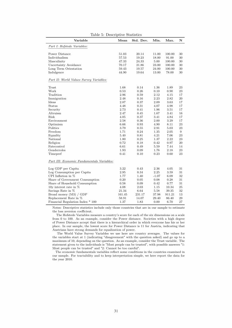
Table 5: Descriptive StatisticsVariable Mean Std. Dev. Min. Max. N

Part I: Hofstede Variables:

Power Distance 51.03 20.14 11.00 100.00 30Individualism 57.53 19.23 18.00 91.00 30Masculinity 47.33 24.33 5.00 100.00 30Uncertainty Avoidance 70.17 21.86 23.00 100.00 30Long Term Orientation 59.43 19.57 24.00 100.00 30Indulgence 44.90 19.64 13.00 78.00 30

Part II: World Values Survey Variables:

Trust 1.68 0.14 1.36 1.89 23Work 0.53 0.26 0.10 0.90 23Tradition 2.96 0.59 2.12 4.15 17Immigration 2.48 0.16 2.23 2.82 20Ideas 2.87 0.37 2.09 3.63 17Status 4.48 0.31 4.07 4.98 17Security 2.73 0.41 1.96 3.51 17Altruism 2.47 0.45 1.67 3.41 16Risk 4.05 0.37 3.41 4.84 17Environment 2.58 0.36 2.00 3.29 17Optimism 6.66 0.93 4.90 8.11 23Politics 3.79 0.55 2.91 5.03 23Freedom 1.71 0.24 1.35 2.05 9Equality 5.40 0.81 4.21 7.06 23National 1.80 0.25 1.37 2.22 23Religion 0.72 0.18 0.42 0.97 20Fatecontrol 6.61 0.49 5.59 7.44 14Genderroles 1.93 0.09 1.76 2.18 23Timepref 0.41 0.10 0.23 0.60 23

Part III: Economic Fundamentals Variables:

Log GDP per Capita 3.22 0.43 2.36 4.05 31Log Consumption per Capita 2.95 0.34 2.25 3.59 31CPI Inflation in % 1.77 1.40 -1.07 6.09 32Share of Government Consumption 0.20 0.05 0.08 0.28 31Share of Household Consumption 0.58 0.09 0.42 0.77 3110y interest rate in % 4.08 2.03 1.15 10.34 25Savings Rate in % 21.34 6.64 5.58 39.35 32Broad money (M3) / GDP 161.45 231.17 37.98 911.21 13Replacement Rate in % 58.91 14.07 29.40 86.40 29Financial Regulation Index * 100 1.37 1.83 0.00 6.70 27

Notes: Descriptive statistics include only those countries that are in our sample to estimatethe loss aversion coefficient.

The Hofstede Variables measure a country’s score for each of the six dimensions on a scalefrom 0 to 100. As an example, consider the Power distance. Societies with a high degreeof Power Distance accept that there is a hierarchical order in which everyone has his or herplace. In our sample, the lowest score for Power Distance is 11 for Austria, indicating thatAustrians have strong demands for equalization of power.

The World Value Survey Variables we use here are country averages. The values forthe variables start at 1 (indicating "disagreement" with the question asked) and go up to amaximum of 10, depending on the question. As an example, consider the Trust variable. Thestatement given to the individuals is "Most people can be trusted", with possible answers "1:Most people can be trusted" and "2: Cannot be too careful".

The economic fundamentals variables reflect some conditions in the countries examined inour sample. For tractability and to keep interpretation simple, we here report the data forthe year 2010.

31

32

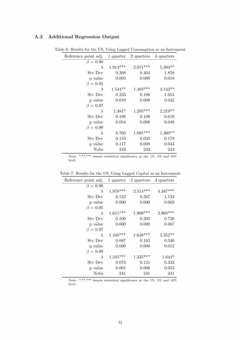
A.2 Additional Regression Output

Table 6: Results for the US, Using Lagged Consumption as an InstrumentReference point adj. 1 quarter 2 quarters 4 quarters

β = 0.90λ 1.914*** 2.071*** 5.394**

Stv Dev 0.308 0.404 1.858p value 0.003 0.008 0.018

β = 0.95λ 1.544** 1.493*** 3.143**

Stv Dev 0.233 0.186 1.054p value 0.019 0.008 0.042

β = 0.97λ 1.381* 1.285*** 2.219**

Stv Dev 0.198 0.108 0.619p value 0.054 0.008 0.049

β = 0.99λ 0.760 1.091*** 1.360**

Stv Dev 0.153 0.035 0.178p value 0.117 0.008 0.043


Table 7: Results for the US, Using Lagged Capital as an InstrumentReference point adj. 1 quarter 2 quarters 4 quarters

β = 0.90λ 1.978*** 2.514*** 4.387***

Stv Dev 0.132 0.307 1.134p value 0.000 0.000 0.003

β = 0.95λ 1.611*** 1.909*** 2.968***

Stv Dev 0.100 0.205 0.726p value 0.000 0.000 0.007

β = 0.97λ 1.448*** 1.648*** 2.352**

Stv Dev 0.087 0.165 0.540p value 0.000 0.000 0.012

β = 0.99λ 1.245*** 1.335*** 1.644*

Stv Dev 0.073 0.121 0.333p value 0.001 0.006 0.053


32

33

A.3 Loss Aversion for Different Sub-Samples

Table 8: Estimated Loss Aversion for Different Sub-SamplesMean St.Dev.

β Lag Nobs Pre-2000 Post-2000 Pre-2000 Post-2000 p-Value0.90 1 23 1.98 1.83 0.26 0.17 0.060.90 2 23 2.52 2.30 0.58 0.49 0.430.90 4 20 3.55 3.09 1.31 1.42 0.730.95 1 23 1.60 1.52 0.16 0.11 0.050.95 2 23 1.90 1.79 0.37 0.30 0.300.95 4 20 2.48 2.26 0.73 0.75 0.900.97 1 23 1.44 1.38 0.12 0.08 0.040.97 2 23 1.64 1.57 0.28 0.22 0.210.97 4 20 2.03 1.90 0.49 0.50 0.930.99 1 23 1.10 1.07 0.22 0.19 0.560.99 2 23 1.33 1.25 0.19 0.22 0.520.99 4 20 1.50 1.47 0.23 0.31 0.23

Notes: The table reports an overview of the point-estimates for the different countries. Forexample, in the column Mean Pre-2000, the cross-country mean of the estimated loss aversioncoefficient for the years prior to 2000 is reported, while St.Dev. reports the standard deviationacross the cross-country estimates. p-Value reports the p-value from a variance comparison testin which the tested hypothesis is that the standard deviations are not the same.Extreme outliers have been removed from the sample.

Table 9: Estimated Loss Aversion for Different Sub-Samples: Euro Area CountriesMean St.Dev.

β Lag Nobs Pre-2000 Post-2000 Pre-2000 Post-2000 p-Value0.90 1 17 1.97 1.77 0.27 0.13 0.010.90 2 17 2.49 2.21 0.63 0.41 0.100.90 4 15 3.48 3.04 1.49 1.55 0.890.95 1 17 1.60 1.49 0.17 0.09 0.010.95 2 17 1.89 1.74 0.41 0.25 0.060.95 4 15 2.43 2.24 0.83 0.82 0.980.97 1 17 1.43 1.36 0.13 0.07 0.010.97 2 17 1.63 1.53 0.32 0.19 0.040.97 4 15 1.99 1.90 0.56 0.55 0.960.99 1 17 1.12 1.05 0.21 0.18 0.510.99 2 17 1.33 1.22 0.22 0.23 0.870.99 4 15 1.48 1.47 0.26 0.34 0.32

Notes: The table reports an overview of the point-estimates for the different countries. Forexample, in the column Mean Pre-2000, the cross-country mean of the estimated loss aversioncoefficient for the years prior to 2000 is reported, while St.Dev. reports the standard deviationacross the cross-country estimates. p-Value reports the p-value from a variance comparison testin which the tested hypothesis is that the standard deviations are not the same.Extreme outliers have been removed from the sample.

33

34

Figure 8: Estimated Loss Aversion Before and After 2000

Notes: The figure in the top (bottom) panel shows results for semi-annual (annual) reference point updating. Thesignificance classification is taken from the estimation where we use the full sample.

34

35

A.4 Robustness of the estimates with respect to the capital share

Figure 9: Estimated Loss Aversion Across Countries: Robustness

Note: The figure in the top (bottom) panel shows results for α = 0.2 (α = 0.5). For both figures, we use an annualupdating of the reference point.

35

36

Recent SNB Working Papers

2018-1 RetoFoellmi,AdrianJaeggiandRinaRosenblatt-Wisch: Loss Aversion at the Aggregate Level Across Countries and its Relation to Economic Fundamentals 2017-18 GregorBäurle,SarahM.LeinandElizabethSteiner: Employment Adjustment and Financial Constraints – Evidence from Firm-level Data

2017-17 ThomasLustenbergerandEnzoRossi: TheSocialValueofInformation: A Test of a Beauty and Non-Beauty Contest

2017-16 AleksanderBerentsenandBenjaminMüller: A Tale of Fire-Sales and Liquidity Hoarding

2017-15 AdrielJost: IsMonetaryPolicyTooComplexforthePublic? Evidence from the UK

2017-14 DavidR.Haab,ThomasNitschka: Predicting returns on asset markets of a small, open economyandtheinfluenceofglobalrisks

2017-13 MathieuGrobéty: GovernmentDebtandGrowth:TheRoleofLiquidity

2017-12 ThomasLustenbergerandEnzoRossi: Does Central Bank Transparency and Communication AffectFinancialandMacroeconomicForecasts? 2017-11 AndreasM.Fischer,RafaelGremingerandChristian Grisse:Portfoliorebalancingintimesofstress

2017-10 ChristianGrisseandSilvioSchumacher:Theresponse oflong-termyieldstonegativeinterestrates:evidence fromSwitzerland

2017-9 PetraGerlach-Kristen,RichhildMoessnerandRina Rosenblatt-Wisch:Computinglong-termmarket inflationexpectationsforcountrieswithoutinflation expectation markets

2017-8 AlainGalli:Whichindicatorsmatter?Analyzingthe Swiss business cycle using a large-scale mixed- frequency dynamic factor model

2017-7 GregorBäurle,MatthiasGublerandDiegoR.Känzig: Internationalinflationspillovers-theroleofdifferent shocks

2017-6 LucasMarcFuhrer:LiquidityintheRepoMarket

2017-5 ChristianGrisse,SigneKrogstrupandSilvio Schumacher:Lowerboundbeliefsandlong-term interest rates

2017-4 ToniBeutler,RobertBichsel,AdrianBruhinandJayson Danton:TheImpactofInterestRateRiskonBank Lending

2017-3 RaphaelA.Auer,AndreiA.LevchenkoandPhilipSauré: InternationalInflationSpilloversThroughInput Linkages

2017-2 AlainGalli,ChristianHepenstrickandRolfScheufele: Mixed-frequencymodelsfortrackingshort-term economicdevelopmentsinSwitzerland

2017-1 MatthiasGublerandChristophSax: TheBalassa-SamuelsonEffectReversed: New Evidence from OECD Countries

2016-19 JensH.E.ChristensenandSigneKrogstrup:APortfolio ModelofQuantitativeEasing

loss aversion at the aggregate level across countries and ... · pdf filereto foellmi, adrian...

Documents