logic programmingdg/teaching/lis2014/modules/lp-fp-07.pdf · logic programming l1.3 a false (a is...
TRANSCRIPT
Logic Programming
Frank PfenningCarnegie Mellon University
Draft of January 2, 2007
Notes for a course given at Carnegie Mellon University, Fall 2006. Mate-rials available at http://www.cs.cmu.edu/~fp/courses/lp. Please sendcomments to [email protected].
Copyright c© Frank Pfenning 2006–2007

LECTURE NOTES JANUARY 2, 2007
15-819K: Logic Programming
Lecture 1
Logic Programming
Frank Pfenning
August 29, 2006
In this first lecture we give a brief introduction to logic programming. Wealso discuss administrative details of the course, although these are notincluded here, but can be found on the course web page.1
1.1 Computation vs. Deduction
Logic programming is a particular way to approach programming. Otherparadigms we might compare it to are imperative programming or func-tional programming. The divisions are not always clear-cut—a functionallanguage may have imperative aspects, for example—but the mindset ofvarious paradigms is quite different and determines how we design andreason about programs.
To understand logic programming, we first examine the difference be-tween computation and deduction. To compute we start from a given ex-pression and, according to a fixed set of rules (the program) generatee aresult. For example, 15 + 26 → (1 + 2 + 1)1 → (3 + 1)1 → 41. To deducewe start from a conjecture and, according to a fixed set of rules (the axiomsand inference rules), try to construct a proof of the conjecture. So computa-tion is mechanical and requires no ingenuity, while deduction is a creativeprocess. For example, an + bn 6= cn for n > 2, . . . 357 years of hard work . . .,QED.
Philosophers, mathematicians, and computer scientists have tried tounify the two, or at least to understand the relationship between them forcenturies. For example, George Boole2 succeeded in reducing a certain class
1http://www.cs.cmu.edu/~fp/courses/lp/21815–1864
LECTURE NOTES AUGUST 29, 2006
L1.2 Logic Programming
of logical reasoning to computation in so-called Boolean algebras. Since thefundamental undecidability results of the 20th centuries we know that noteverything we can reason about is in fact mechanically computable, even ifwe follow a well-defined set of formal rules.
In this course we are interested in a connection of a different kind. Afirst observation is that computation can be seen as a limited form of de-duction because it establishes theorems. For example, 15 + 26 = 41 is boththe result of a computation, and a theorem of arithmetic. Conversely, de-duction can be considered a form of computation if we fix a strategy forproof search, removing the guesswork (and the possibility of employingingenuity) from the deductive process.
This latter idea is the foundation of logic programming. Logic programcomputation proceeds by proof search according to a fixed strategy. Byknowing what this strategy is, we can implement particular algorithms inlogic, and execute the algorithms by proof search.
1.2 Judgments and Proofs
Since logic programming computation is proof search, to study logic pro-gramming means to study proofs. We adopt here the approach by Martin-Lof [3]. Although he studied logic as a basis for functional programmingrather than logic programming, his ideas are more fundamental and there-fore equally applicable in both paradigms.
The most basic notion is that of a judgment, which is an object of knowl-edge. We know a judgment because we have evidence for it. The kind ofevidence we are most interested in is a proof, which we display as a deduc-tion using inference rules in the form
J1 . . . Jn
JR
where R is the name of the rule (often omitted), J is the judgment estab-lished by the inference (the conclusion), and J1, . . . , Jn are the premisses ofthe rule. We can read it as
If J1 and · · · and Jn then we can conclude J by virtue of rule R.
By far the most common judgment is the truth of a proposition A, whichwe write as A true . Because we will be occupied almost exclusively withthe thruth of propositions for quite some time in this course we generallyomit the trailing “true”. Other examples of judgments on propositions are
LECTURE NOTES AUGUST 29, 2006
Logic Programming L1.3
A false (A is false), A true at t (A is true at time t, the subject of temporallogic), or K knows A (K knows that A is true, the subject of epistemic logic).
To give some simple examples we need a language to express propo-sitions. We start with terms t that have the form f(t1, . . . , tn) where f is afunction symbol of arity n and t1, . . . , tn are the arguments. Terms can havevariables in them, which we generally denote by upper-case letters. Atomicpropositions P have the form p(t1, . . . , tn) where p is a predicate symbol of ar-ity n and t1, . . . , tn are its arguments. Later we will introduce more generalforms of propositions, built up by logical connectives and quantifiers fromatomic propositions.
In our first set of examples we represent natural numbers 0, 1, 2, . . . asterms of the form z, s(z), s(s(z)), . . ., using two function symbols (z of arity0 and s of arity 1).3 The first predicate we consider is even of arity 1. Itsmeaning is defined by two inference rules:
even(z)evz
even(N)
even(s(s(N)))evs
The first rule, evz, expresses that 0 is even. It has no premiss and therefore islike an axiom. The second rule, evs, expresses that if N is even, then s(s(N))is also even. Here, N is a schematic variable of the inference rule: everyinstance of the rule where N is replaced by a concrete term represents avalid inference. We have no more rules, so we think of these two as definingthe predicate even completely.
The following is a trivial example of a deduction, showing that 4 is even:
even(z)evz
even(s(s(z)))evs
even(s(s(s(s(z)))))evs
Here, we used the rule evs twice: once with N = z and once with N =s(s(z)).
1.3 Proof Search
To make the transition from inference rules to logic programming we needto impose a particular strategy. Two fundamental ideas suggest them-selves: we could either search backward from the conjecture, growing a
3This is not how numbers are represented in practical logic programming languagessuch as Prolog, but it is a convenient source of examples.
LECTURE NOTES AUGUST 29, 2006
L1.4 Logic Programming
(potential) proof tree upwards, or we could work forwards from the ax-ioms applying rules until we arrive at the conjecture. We call the first onegoal-directed and the second one forward-reasoning. In the logic program-ming literature we find the terminology top-down for goal-directed, andbottom-up for forward-reasoning, but this goes counter to the direction inwhich the proof tree is constructed. Logic programming was conceivedwith goal-directed search, and this is still the dominant direction since itunderlies Prolog, the most popular logic programming language. Later inthe class, we will also have an opportunity to consider forward reasoning.
In the first approximation, the goal-directed strategy we apply is verysimple: given a conjecture (called the goal) we determine which inferencerules might have been applied to arrive at this conclusion. We select one ofthem and then recursively apply our strategy to all the premisses as sub-goals. If there are no premisses we have completed the proof of the goal.We will consider many refinements and more precise descriptions of searchin this course.
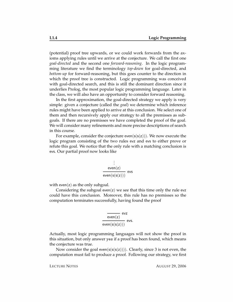
For example, consider the conjecture even(s(s(z))). We now execute thelogic program consisting of the two rules evz and evs to either prove orrefute this goal. We notice that the only rule with a matching conclusion isevs. Our partial proof now looks like
...even(z)
even(s(s(z)))evs
with even(z) as the only subgoal.Considering the subgoal even(z) we see that this time only the rule evz
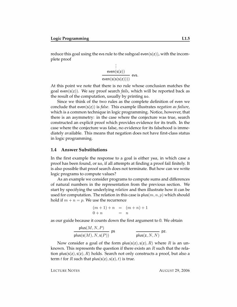
could have this conclusion. Moreover, this rule has no premisses so thecomputation terminates successfully, having found the proof
even(z)evz
even(s(s(z)))evs.
Actually, most logic programming languages will not show the proof inthis situation, but only answer yes if a proof has been found, which meansthe conjecture was true.
Now consider the goal even(s(s(s(z)))). Clearly, since 3 is not even, thecomputation must fail to produce a proof. Following our strategy, we first
LECTURE NOTES AUGUST 29, 2006
Logic Programming L1.5
reduce this goal using the evs rule to the subgoal even(s(z)), with the incom-plete proof
...even(s(z))
even(s(s(s(z))))evs.
At this point we note that there is no rule whose conclusion matches thegoal even(s(z)). We say proof search fails, which will be reported back asthe result of the computation, usually by printing no.
Since we think of the two rules as the complete definition of even weconclude that even(s(z)) is false. This example illustrates negation as failure,which is a common technique in logic programming. Notice, however, thatthere is an asymmetry: in the case where the conjecture was true, searchconstructed an explicit proof which provides evidence for its truth. In thecase where the conjecture was false, no evidence for its falsehood is imme-diately available. This means that negation does not have first-class statusin logic programming.
1.4 Answer Substitutions
In the first example the response to a goal is either yes, in which case aproof has been found, or no, if all attempts at finding a proof fail finitely. Itis also possible that proof search does not terminate. But how can we writelogic programs to compute values?
As an example we consider programs to compute sums and differencesof natural numbers in the representation from the previous section. Westart by specifying the underlying relation and then illustrate how it can beused for computation. The relation in this case is plus(m,n, p) which shouldhold if m + n = p. We use the recurrence
(m + 1) + n = (m + n) + 10 + n = n
as our guide because it counts down the first argument to 0. We obtain
plus(M,N,P )
plus(s(M), N, s(P ))ps
plus(z,N,N)pz.
Now consider a goal of the form plus(s(z), s(z), R) where R is an un-known. This represents the question if there exists an R such that the rela-tion plus(s(z), s(z), R) holds. Search not only constructs a proof, but also aterm t for R such that plus(s(z), s(z), t) is true.
LECTURE NOTES AUGUST 29, 2006
L1.6 Logic Programming
For the original goal, plus(s(z), s(z), R), only the rule ps could apply be-cause of a mismatch between z and s(z) in the first argument to plus in theconclusion. We also see that the R must have the form s(P ) for some P ,although we do not know yet what P should be.
...plus(z, s(z), P )
plus(s(z), s(z), R)ps with R = s(P )
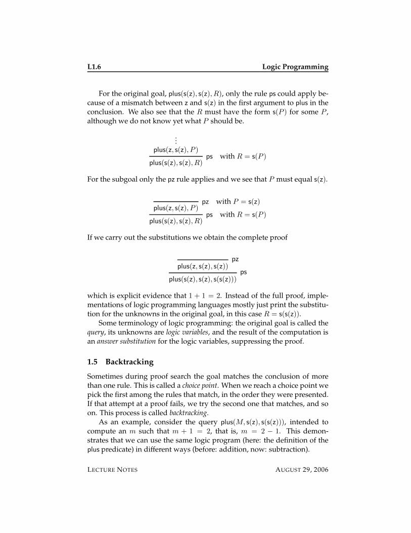
For the subgoal only the pz rule applies and we see that P must equal s(z).
plus(z, s(z), P )pz with P = s(z)
plus(s(z), s(z), R)ps with R = s(P )
If we carry out the substitutions we obtain the complete proof
plus(z, s(z), s(z))pz
plus(s(z), s(z), s(s(z)))ps
which is explicit evidence that 1 + 1 = 2. Instead of the full proof, imple-mentations of logic programming languages mostly just print the substitu-tion for the unknowns in the original goal, in this case R = s(s(z)).
Some terminology of logic programming: the original goal is called thequery, its unknowns are logic variables, and the result of the computation isan answer substitution for the logic variables, suppressing the proof.
1.5 Backtracking
Sometimes during proof search the goal matches the conclusion of morethan one rule. This is called a choice point. When we reach a choice point wepick the first among the rules that match, in the order they were presented.If that attempt at a proof fails, we try the second one that matches, and soon. This process is called backtracking.
As an example, consider the query plus(M, s(z), s(s(z))), intended tocompute an m such that m + 1 = 2, that is, m = 2 − 1. This demon-strates that we can use the same logic program (here: the definition of theplus predicate) in different ways (before: addition, now: subtraction).
LECTURE NOTES AUGUST 29, 2006
Logic Programming L1.7
The conclusion of the rule pz, plus(z,N,N), does not match because thesecond and third argument of the query are different. However, the rule ps
applies and we obtain
...plus(M1, s(z), s(z))
plus(M, s(z), s(s(z)))ps with M = s(M1)
At this point both rules, ps and pz, match. Because the rule ps is listed first,leading to
...plus(M2, s(z), z)
plus(M1, s(z), s(z))ps with M1 = s(M2)
plus(M, s(z), s(s(z)))ps with M = s(M1)
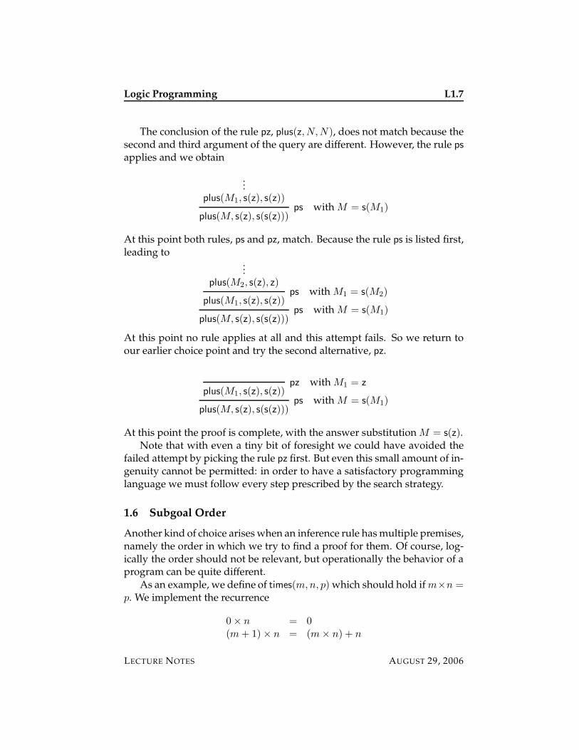
At this point no rule applies at all and this attempt fails. So we return toour earlier choice point and try the second alternative, pz.
plus(M1, s(z), s(z))pz with M1 = z
plus(M, s(z), s(s(z)))ps with M = s(M1)
At this point the proof is complete, with the answer substitution M = s(z).Note that with even a tiny bit of foresight we could have avoided the
failed attempt by picking the rule pz first. But even this small amount of in-genuity cannot be permitted: in order to have a satisfactory programminglanguage we must follow every step prescribed by the search strategy.
1.6 Subgoal Order
Another kind of choice arises when an inference rule has multiple premises,namely the order in which we try to find a proof for them. Of course, log-ically the order should not be relevant, but operationally the behavior of aprogram can be quite different.
As an example, we define of times(m,n, p) which should hold if m×n =p. We implement the recurrence
0× n = 0(m + 1)× n = (m× n) + n
LECTURE NOTES AUGUST 29, 2006
L1.8 Logic Programming
in the form of the following two inference rules.
times(z, N, z)tz
times(M,N,P ) plus(P,N,Q)
times(s(M),N,Q)ts
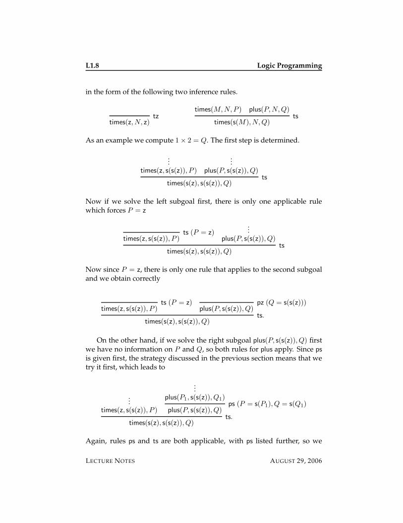
As an example we compute 1× 2 = Q. The first step is determined.
...times(z, s(s(z)), P )
...plus(P, s(s(z)), Q)
times(s(z), s(s(z)), Q)ts
Now if we solve the left subgoal first, there is only one applicable rulewhich forces P = z
times(z, s(s(z)), P )ts (P = z)
...plus(P, s(s(z)), Q)
times(s(z), s(s(z)), Q)ts
Now since P = z, there is only one rule that applies to the second subgoaland we obtain correctly
times(z, s(s(z)), P )ts (P = z)
plus(P, s(s(z)), Q)pz (Q = s(s(z)))
times(s(z), s(s(z)), Q)ts.
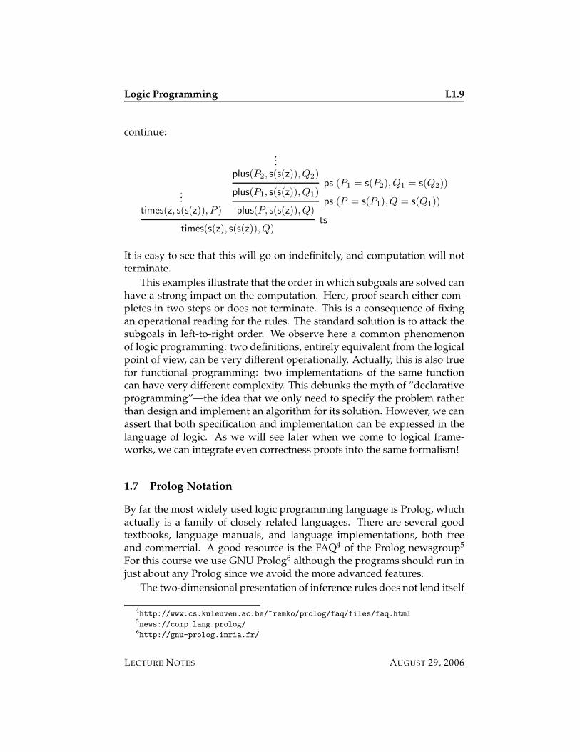
On the other hand, if we solve the right subgoal plus(P, s(s(z)), Q) firstwe have no information on P and Q, so both rules for plus apply. Since ps
is given first, the strategy discussed in the previous section means that wetry it first, which leads to
...times(z, s(s(z)), P )
...plus(P1, s(s(z)), Q1)
plus(P, s(s(z)), Q)ps (P = s(P1), Q = s(Q1)
times(s(z), s(s(z)), Q)ts.
Again, rules ps and ts are both applicable, with ps listed further, so we
LECTURE NOTES AUGUST 29, 2006
Logic Programming L1.9
continue:
...times(z, s(s(z)), P )
...plus(P2, s(s(z)), Q2)
plus(P1, s(s(z)), Q1)ps (P1 = s(P2), Q1 = s(Q2))
plus(P, s(s(z)), Q)ps (P = s(P1), Q = s(Q1))
times(s(z), s(s(z)), Q)ts
It is easy to see that this will go on indefinitely, and computation will notterminate.
This examples illustrate that the order in which subgoals are solved canhave a strong impact on the computation. Here, proof search either com-pletes in two steps or does not terminate. This is a consequence of fixingan operational reading for the rules. The standard solution is to attack thesubgoals in left-to-right order. We observe here a common phenomenonof logic programming: two definitions, entirely equivalent from the logicalpoint of view, can be very different operationally. Actually, this is also truefor functional programming: two implementations of the same functioncan have very different complexity. This debunks the myth of “declarativeprogramming”—the idea that we only need to specify the problem ratherthan design and implement an algorithm for its solution. However, we canassert that both specification and implementation can be expressed in thelanguage of logic. As we will see later when we come to logical frame-works, we can integrate even correctness proofs into the same formalism!
1.7 Prolog Notation
By far the most widely used logic programming language is Prolog, whichactually is a family of closely related languages. There are several goodtextbooks, language manuals, and language implementations, both freeand commercial. A good resource is the FAQ4 of the Prolog newsgroup5
For this course we use GNU Prolog6 although the programs should run injust about any Prolog since we avoid the more advanced features.
The two-dimensional presentation of inference rules does not lend itself
4http://www.cs.kuleuven.ac.be/~remko/prolog/faq/files/faq.html5news://comp.lang.prolog/6http://gnu-prolog.inria.fr/
LECTURE NOTES AUGUST 29, 2006
L1.10 Logic Programming
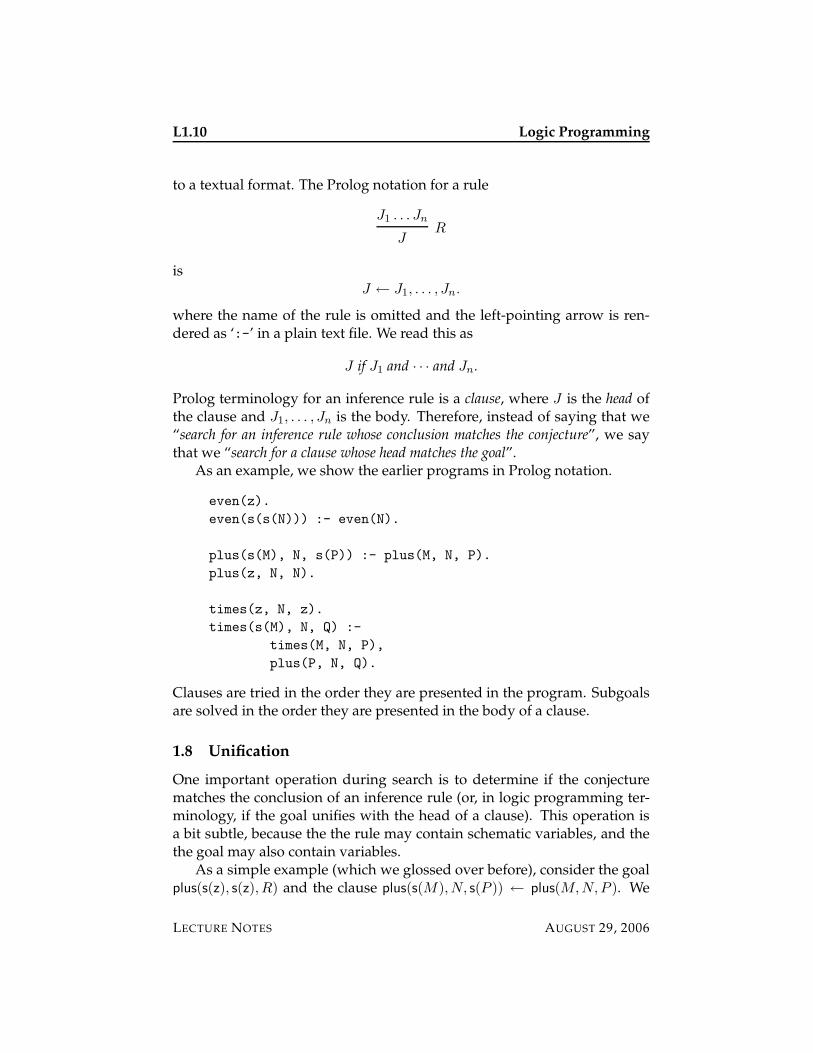
to a textual format. The Prolog notation for a rule
J1 . . . Jn
JR
isJ ← J1, . . . , Jn.
where the name of the rule is omitted and the left-pointing arrow is ren-dered as ‘:-’ in a plain text file. We read this as
J if J1 and · · · and Jn.
Prolog terminology for an inference rule is a clause, where J is the head ofthe clause and J1, . . . , Jn is the body. Therefore, instead of saying that we“search for an inference rule whose conclusion matches the conjecture”, we saythat we “search for a clause whose head matches the goal”.
As an example, we show the earlier programs in Prolog notation.
even(z).
even(s(s(N))) :- even(N).
plus(s(M), N, s(P)) :- plus(M, N, P).
plus(z, N, N).
times(z, N, z).
times(s(M), N, Q) :-
times(M, N, P),
plus(P, N, Q).
Clauses are tried in the order they are presented in the program. Subgoalsare solved in the order they are presented in the body of a clause.
1.8 Unification
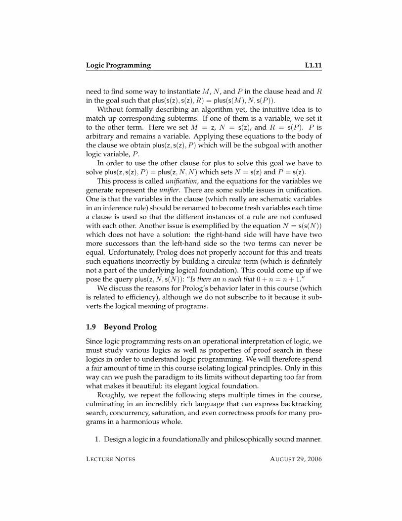
One important operation during search is to determine if the conjecturematches the conclusion of an inference rule (or, in logic programming ter-minology, if the goal unifies with the head of a clause). This operation isa bit subtle, because the the rule may contain schematic variables, and thethe goal may also contain variables.
As a simple example (which we glossed over before), consider the goalplus(s(z), s(z), R) and the clause plus(s(M),N, s(P )) ← plus(M,N,P ). We
LECTURE NOTES AUGUST 29, 2006
Logic Programming L1.11
need to find some way to instantiate M , N , and P in the clause head and R
in the goal such that plus(s(z), s(z), R) = plus(s(M),N, s(P )).
Without formally describing an algorithm yet, the intuitive idea is tomatch up corresponding subterms. If one of them is a variable, we set itto the other term. Here we set M = z, N = s(z), and R = s(P ). P isarbitrary and remains a variable. Applying these equations to the body ofthe clause we obtain plus(z, s(z), P ) which will be the subgoal with anotherlogic variable, P .
In order to use the other clause for plus to solve this goal we have tosolve plus(z, s(z), P ) = plus(z,N,N) which sets N = s(z) and P = s(z).
This process is called unification, and the equations for the variables wegenerate represent the unifier. There are some subtle issues in unification.One is that the variables in the clause (which really are schematic variablesin an inference rule) should be renamed to become fresh variables each timea clause is used so that the different instances of a rule are not confusedwith each other. Another issue is exemplified by the equation N = s(s(N))which does not have a solution: the right-hand side will have have twomore successors than the left-hand side so the two terms can never beequal. Unfortunately, Prolog does not properly account for this and treatssuch equations incorrectly by building a circular term (which is definitelynot a part of the underlying logical foundation). This could come up if wepose the query plus(z, N, s(N)): “Is there an n such that 0 + n = n + 1.”
We discuss the reasons for Prolog’s behavior later in this course (whichis related to efficiency), although we do not subscribe to it because it sub-verts the logical meaning of programs.
1.9 Beyond Prolog
Since logic programming rests on an operational interpretation of logic, wemust study various logics as well as properties of proof search in theselogics in order to understand logic programming. We will therefore spenda fair amount of time in this course isolating logical principles. Only in thisway can we push the paradigm to its limits without departing too far fromwhat makes it beautiful: its elegant logical foundation.
Roughly, we repeat the following steps multiple times in the course,culminating in an incredibly rich language that can express backtrackingsearch, concurrency, saturation, and even correctness proofs for many pro-grams in a harmonious whole.
1. Design a logic in a foundationally and philosophically sound manner.
LECTURE NOTES AUGUST 29, 2006
L1.12 Logic Programming
2. Isolate a fragment of the logic based on proof search criteria.
3. Give an informal description of its operational behavior.
4. Explore programming techniques and idioms.
5. Formalize the operational semantics.
6. Implement a high-level interpreter.
7. Study properties of the language as a whole.
8. Develop techniques for reasoning about individual programs.
9. Identify limitations and consider how they might be addressed, eitherby logical or operational means.
10. Go to step 1.
Some of the logics we will definitely consider are intuitionistic logic,modal logic, higher-order logic, and linear logic, and possibly also tempo-ral and epistemic logics. Ironically, even though logic programming de-rives from logic, the language we have considered so far (which is the basisof Prolog) does not require any logical connectives at all, just the mecha-nisms of judgments and inference rules.
1.10 Historical Notes
Logic programming and the Prolog language are credited to Alain Colmer-auer and Robert Kowalski in the early 1970s. Colmerauer had been work-ing on a specialized theorem prover for natural language processing, whicheventually evolved to a general purpose language called Prolog (for Pro-grammation en Logique) that embodies the operational reading of clausesformulated by Kowalski. Interesting accounts of the birth of logic pro-gramming can be found in papers by the Colmerauer and Roussel [1] andKowalski [2].
We like Sterling and Shapiro’s The Art of Prolog [4] as a good introduc-tory textbook for those who already know how to program and we recom-mends O’Keefe’s The Craft of Prolog as a second book for those aspiring tobecome real Prolog hackers. Both of these are somewhat dated and do notcover many modern developments, which are the focus of this course. Wetherefore do not use them as textbooks here.
LECTURE NOTES AUGUST 29, 2006
Logic Programming L1.13
1.11 Exercises
Exercise 1.1 A different recurrence for addition is
(m + 1) + n = m + (n + 1)0 + n = n
Write logic programs for addition on numbers in unary notation based on thisrecurrence. What kind of query do we need to pose to compute differences correctly?
Exercise 1.2 Determine if the times predicate can be used to calculate exact divi-sion, that is, given m and n find q such that m = n× q and fail if no such q exists.If not, give counterexamples for different ways that times could be invoked andwrite another program divexact to perform exact divison. Also write a program tocalculate both quotient and remainder of two numbers.
Exercise 1.3 We saw that the plus predicate can be used to compute sums and dif-ferences. Find other creative uses for this predicate without writing any additionalcode.
Exercise 1.4 Devise a representation of natural numbers in binary form as terms.Write logic programs to add and multiply binary numbers, and to translate be-tween unary and binary numbers. Can you write a single relation that can beexecuted to translate in both directions?
1.12 References
[1] Alain Colmerauer and Philippe Roussel. The birth of Prolog. In Confer-ence on the History of Programming Languages (HOPL-II), Preprints, pages37–52, Cambridge, Massachusetts, April 1993.
[2] Robert A. Kowalski. The early years of logic programming. Communi-cations of the ACM, 31(1):38–43, 1988.
[3] Per Martin-Lof. On the meanings of the logical constants and the justi-fications of the logical laws. Nordic Journal of Philosophical Logic, 1(1):11–60, 1996.
[4] Leon Sterling and Ehud Shapiro. The Art of Prolog. The MIT Press,Cambridge, Massachusetts, 2nd edition edition, 1994.
LECTURE NOTES AUGUST 29, 2006

L1.14 Logic Programming
LECTURE NOTES AUGUST 29, 2006
15-819K: Logic Programming
Lecture 2
Data Structures
Frank Pfenning
August 31, 2006
In this second lecture we introduce some simple data structures such aslists, and simple algorithms on them such as as quicksort or mergesort.We also introduce some first considerations of types and modes for logicprograms.
2.1 Lists
Lists are defined by two constructors: the empty list nil and the constructorcons which takes an element and a list, generating another list. For exam-ple, the list a, b, c would be represented as cons(a, cons(b, cons(c, nil))). Theofficial Prolog notation for nil is [], and for cons(h, t) is .(h, t), overload-ing the meaning of the period ‘.’ as a terminator for clauses and a binaryfunction symbol. In practice, however, this notation for cons is rarely used.Instead, most Prolog programs use [h|t] for cons(h, t).
There is also a sequence notation for lists, so that a, b, c can be writ-ten as [a, b, c]. It could also be written as [a | [b | [c | []]]] or[a, b | [c, []]]. Note that all of these notations will be parsed into thesame internal form, using nil and cons. We generally follow Prolog list no-tation in these notes.
2.2 Type Predicates
We now return to the definition of plus from the previous lecture, exceptthat we have reversed the order of the two clauses.
plus(z, N, N).
plus(s(M), N, s(P)) :- plus(M, N, P).
LECTURE NOTES AUGUST 31, 2006
L2.2 Data Structures
In view of the new list constructors for terms, the first clause now lookswrong. For example, with this clause we can prove
plus(s(z), [a, b, c], s([a, b, c])).
This is absurd: what does it mean to add 1 and a list? What does the terms([a, b, c]) denote? It is clearly neither a list nor a number.
From the modern programming language perspective the answer isclear: the definition above lacks types. Unfortunately, Prolog (and tradi-tional predicate calculus from which it was originally derived) do not dis-tinguish terms of different types. The historical answer for why these lan-guages have just a single type of terms is that types can be defined as unarypredicates. While this is true, it does not account for the pragmatic advan-tage of distinguishing meaningful propositions from those that are not. Toillustrate this, the standard means to correct the example above would beto define a predicate nat with the rules
nat(z)nz
nat(N)
nat(s(N))ns
and modify the base case of the rules for addition
nat(N)
plus(z, N,N)pz
plus(M,N,P )
plus(s(M),N, s(P ))ps
One of the problems is that now, for example, plus(z, nil, nil) is false, when itshould actually be meaningless. Many problems in debugging Prolog pro-grams can be traced to the fact that propositions that should be meaninglesswill be interpreted as either true or false instead, incorrectly succeeding orfailing. If we transliterate the above into Prolog, we get:
nat(z).
nat(s(N)) :- nat(N).
plus(z, N, N) :- nat(N).
plus(s(M), N, s(P)) :- plus(M, N, P).
No self-respecting Prolog programmer would write the plus predicate thisway. Instead, he or she would omit the type test in the first clause leadingto the earlier program. The main difference between the two is whethermeaningless clauses are false (with the type test) or true (without the typetest). One should then annotate the predicate with the intended domain.
LECTURE NOTES AUGUST 31, 2006
Data Structures L2.3
% plus(m, n, p) iff m + n = p for nat numbers m, n, p.
plus(z, N, N).
plus(s(M), N, s(P)) :- plus(M, N, P).
It would be much preferable from the programmer’s standpoint if thisinformal comment were a formal type declaration, and an illegal invocationof plus were a compile-time error rather than leading to silent success orfailure. There has been some significant research on types systems and typechecking for logic programming languages [5] and we will talk about typesmore later in this course.
2.3 List Types
We begin with the type predicates defining lists.
list([]).
list([X|Xs]) :- list(Xs).
Unlike languages such as ML, there is no test whether the elements of a listall have the same type. We could easily test whether something is a list ofnatural numbers.
natlist([]).
natlist([N|Ns]) :- nat(N), natlist(Ns).
The generic test, whether we are presented with a homogeneous list, all ofwhose elements satisfy some predicate P, would be written as:
plist(P, []).
plist(P, [X|Xs]) :- P(X), plist(P, Xs).
While this is legal in some Prolog implementations, it can not be justifiedfrom the underlying logical foundation, because P stands for a predicateand is an argument to another predicate, plist. This is the realm of higher-order logic, and a proper study of it requires a development of higher-orderlogic programming [3, 4]. In Prolog the goal P(X) is a meta-call, often writtenas call(P(X)). We will avoid its use, unless we develop higher-order logicprogramming later in this course.
2.4 List Membership and Disequality
As a second example, we consider membership of an element in a list.
member(X, cons(X,Y s))
member(X,Y s)
member(X, cons(Y, Y s))
LECTURE NOTES AUGUST 31, 2006
L2.4 Data Structures
In Prolog syntax:
% member(X, Ys) iff X is a member of list Ys
member(X, [X|Ys]).
member(X, [Y|Ys]) :- member(X, Ys).
Note that in the first clause we have omitted the check whether Ys is aproper list, making it part of the presupposition that the second argumentto member is a list.
Already, this very simple predicate has some subtle points. To showthe examples, we use the Prolog notation ?- A. for a query A. After pre-senting the first answer substitution, Prolog interpreters issue a prompt tosee if another solution is desired. If the user types ‘;’ the interpreter willbacktrack to see if another solution can be found. For example, the query
?- member(X, [a,b,a,c]).
has four solutions, in the order
X = a;
X = b;
X = a;
X = c.
Perhaps surprisingly, the query
?- member(a, [a,b,a,c]).
succeeds twice (both with the empty substitution), once for the first occur-rence of a and once for the second occurrence.
If member is part of a larger program, backtracking of a later goal couldlead to unexpected surprises when member succeeds again. There couldalso be an efficiency issue. Assume you keep the list in alphabetical order.Then when we find the first matching element there is no need to traversethe remainder of the list, although the member predicate above will alwaysdo so.
So what do we do if we want to only check membership, or find the firstoccurrence of an element in a list? Unfortunately, there is no easy answer,because the most straighforward solution
member(X, cons(X,Y s))
X 6= Y member(X,Y s)
member(X, cons(Y, Y s))
requires disequality which is problematic in the presence of variables. InProlog notation:
LECTURE NOTES AUGUST 31, 2006
Data Structures L2.5
member1(X, [X|Ys]).
member1(X, [Y|Ys]) :- X \= Y, member1(X, Ys).
When both arguments are ground, this works as expected, giving just onesolution to the query
?- member1(a, [a,b,a,c]).
However, when we ask
?- member1(X, [a,b,a,c]).
we only get one answer, namely X = a. The reason is that when we cometo the second clause, we instantiate Y to a and Ys to [b,a,c], and the bodyof the clause becomes
X \= a, member1(X, [b,a,c]).
Now we have the problem that we cannot determine if X is different froma, because X is still a variable. Prolog interprets s 6= t as non-unifiability, thatis, s 6= t succeeds of s and t are not unifiable. But X and a are unifiable, sothe subgoal fails and no further solutions are generated.1
There are two attitudes we can take. One is to restrict the use of dis-equality (and, therefore, here also the use of member1) to the case whereboth sides have no variables in them. In that case disequality can be easilychecked without problems. This is the solution adopted by Prolog, and onewhich we adopt for now.
The second one is to postpone the disequality s 6= t until we can tellfrom the structure of s and t that they will be different (in which case wesucceed) or the same (in which case the disequality fails). The latter so-lution requires a much more complicated operational semantics becausesome goals must be postponed until their arguments become instantiated.This is the general topic of constructive negation2 [1] in the setting of con-straint logic programming [2, 6], which we will address later in the course.
Disequality is related to the more general question of negation, becauses 6= t is the negation of equality, which is a simple predicate that is eitherprimitive, or could be defined with the one clause X = X.
1One must remember, however, that in Prolog unification is not sound because it omitsthe occurs-check, as hinted at in the previous lecture. This also affects the correctness ofdisequality.
2The use of the word “constructive” here is unrelated to its use in logic.
LECTURE NOTES AUGUST 31, 2006
L2.6 Data Structures
2.5 Simple List Predicates
After the member predicate generated some interesting questions, we ex-plore some other list operations. We start with prefix(xs, ys) which is sup-posed to hold when the list xs is a prefix of the list ys. The definition isrelatively straightforward.
prefix([], Ys).
prefix([X|Xs], [X|Ys]) :- prefix(Xs, Ys).
Conversely, we can test for a suffix.
suffix(Xs, Xs).
suffix(Xs, [Y|Ys]) :- suffix(Xs, Ys).
Interestingly, these predicates can be used in a variety of ways. We cancheck is one list is a prefix of another, we can enumerate prefixes, and wecan even enumerate prefixes and lists. For example:
?- prefix(Xs,[a,b,c,d]).
Xs = [];
Xs = [a];
Xs = [a,b];
Xs = [a,b,c];
Xs = [a,b,c,d].
enumerates all prefixes, while
?- prefix(Xs,Ys).
Xs = [];
Xs = [A]
Ys = [A|_];
Xs = [A,B]
Ys = [A,B|_];
Xs = [A,B,C]
Ys = [A,B,C|_];
Xs = [A,B,C,D]
Ys = [A,B,C,D|_];
...
LECTURE NOTES AUGUST 31, 2006
Data Structures L2.7
enumerates lists together with prefixes. Note that A, B, C, and D are vari-ables, as is the underscore _ so that for example [A|_] represents any listwith at least one element.
A more general prediate is append(xs, ys, zs) which holds when zs isthe result of appending xs and ys.
append([], Ys, Ys).
append([X|Xs], Ys, [X|Zs]) :- append(Xs, Ys, Zs).
append can also be used in different directions, and we can also employ itfor alternative definitions of prefix and suffix.
prefix2(Xs, Ys) :- append(Xs, _, Ys).
suffix2(Xs, Ys) :- append(_, Xs, Ys).
Here we have used anonymous variables ‘_’. Note that when several un-derscores appear in a clauses, each one stands for a different anonymousvariable. For example, if we want to define a sublist as a suffix of a pre-fix, we have to name the intermediate variable instead of leaving it anony-mous.
sublist(Xs, Ys) :- prefix(Ps, Ys), suffix(Xs, Ps).
This definition of sublist has some shortcomings (see Exercise 2.1).
2.6 Sorting
As a slightly larger example, we use a recursive definition of quicksort.This is particularly instructive as it clarifies the difference between a speci-fication and an implemention. A specification for sort(xs, ys) would simplysay that ys is an ordered permutation of xs. However, this specification isnot useful as an implementation: we do not want to cycle through all pos-sible permutations until we find one that is ordered.
Instead we implement a non-destructive version of quicksort, modeledafter similar implementations in functional programming. We use here thebuilt-in Prolog integers, rather than the unary representation from the pre-vious lecture. Prolog integers can be compared with n =< m (n is less orequal to m) and n > m (n is greater than m) and similar predicates, writ-ten in infix notation. In order for these comparisons to make sense, thearguments must be instantiated to actual integers and are not allowed tobe variables, which constitute a run-time error. This combines two condi-tions: one which is called a mode is that =< and < require their arguments
LECTURE NOTES AUGUST 31, 2006
L2.8 Data Structures
to be ground upon invocation, that is not contain any variables. The secondcondition is a type condition which requires the arguments to be integers.Since these conditions can not be enforced at compile time, they are sig-naled as run-time errors.
Quicksort proceeds by partitioning the tail of the input list into thoseelements that are smaller than or equal to its first element and those thatare larger than its first element. It then recursively sorts the two sublistsand appends the results.
quicksort([], []).
quicksort([X0|Xs], Ys) :-
partition(Xs, X0, Ls, Gs),
quicksort(Ls, Ys1),
quicksort(Gs, Ys2),
append(Ys1, [X0|Ys2], Ys).
Partitioning a list about the pivot element X0 is also straightforward.
partition([], _, [], []).
partition([X|Xs], X0, [X|Ls], Gs) :-
X =< X0, partition(Xs, X0, Ls, Gs).
partition([X|Xs], X0, Ls, [X|Gs]) :-
X > X0, partition(Xs, X0, Ls, Gs).
Note that the second and third case are both guarded by comparisons. Thiswill fail if either X or X0 are uninstantiated or not integers. The predicatepartition(xs, x0, ls, gs) therefore inherits a mode and type restric-tion: the first argument must be a ground list of integers and the secondargument must be a ground integer. If these conditions are satisfied andpartition succeeds, the last two arguments will always be lists of groundintegers. In a future lecture we will discuss how to enforce conditions ofthis kind to discover bugs early. Here, the program is small, so we can getby without mode checking and type checking.
It may seem that the check X > X0 in the last clause is redundant. How-ever, that is not the case because upon backtracking we might select thesecond clause, even if the first one succeeded earlier, leading to an incor-rect result. For example, without this guard the query
?- quicksort([2,1,3], Ys)
would incorrectly return Ys = [2,1,3] as its second solution.
LECTURE NOTES AUGUST 31, 2006
Data Structures L2.9
In this particular case, the test is trivial so the overhead is acceptable.Sometimes, however, a clause is guarded by a complicated test which takesa long time to evaluate. In that case, there is no easy way to avoid evaluat-ing it twice, in pure logic programming. Prolog offers several ways to workaround this limitation which we discuss in the next section.
2.7 Conditionals
We use the example of computing the minimum of two numbers as an ex-ample analogous to partition, but shorter.
minimum(X, Y, X) :- X =< Y.
minimum(X, Y, Y) :- X > Y.
In order to avoid the second, redundant test we can use Prolog’s condi-tional construct, written as
A -> B ; C
which solves goal A. If A succeeds we commit to the solution, removingall choice points created during the search for a proof of A and then solveB. If A fails we solve C instead. There is also a short form A -> B which isequivalent to A -> B ; fail where fail is a goal that always fails.
Using the conditional, minimum can be rewritten more succinctly as
minimum(X, Y, Z) :- X =< Y -> Z = X ; Z = Y.
The price that we pay here is that we have to leave the realm of pure logicprogramming.
Because the conditional is so familiar from imperative and functionalprogram, there may be a tendency to overuse the conditional when it caneasily be avoided.
2.8 Cut
The conditional combines two ideas: commiting to all choices so that onlythe first solution to a goal will be considered, and branching based on thatfirst solution.
A more powerful primitive is cut, written as ‘!’, which is unrelated tothe use of the word “cut” in proof theory. A cut appears in a goal positionand commits to all choices that have been made since the clause it appearsin has been selected, including the choice of that clause. For example, thefollowing is a correct implementation of minimum in Prolog.
LECTURE NOTES AUGUST 31, 2006
L2.10 Data Structures
minimum(X, Y, Z) :- X =< Y, !, Z = X.
minimum(X, Y, Y).
The first clause states that if x is less or equal to y than the minimum is equalto x. Moreover, we commit to this clause in the definition of minimum andon backtracking we do not attempt to use the second clause (which wouldotherwise be incorrect, of course).
If we permit meta-calls in clauses, then we can define the conditionalA -> B ; C using cut with
if_then_else(A, B, C) :- A, !, B.
if_then_else(A, B, C) :- C.
The use of cut in the first clause removes all choice points created duringthe search for a proof of A when it succeeds for the first time, and alsocommits to the first clause of if_then_else. The solution of B will createchoice points and backtrack as usual, except when it fails the second clauseof if_then_else will never be tried.
If A fails before the cut, then the second clause will be tried (we haven’tcommitted to the first one) and C will be executed.
Cuts can be very tricky and are the source of many errors, because theirinterpretation depends so much on the operational behavior of the pro-gram rather than the logical reading of the program. One should resist thetemptation to use cuts excessively to improve the efficiency of the programunless it is truly necessary.
Cuts are generally divided into green cuts and red cuts. Green cuts aremerely for efficiency, to remove redundant choice points, while red cutschange the meaning of the program entirely. Revisiting the earlier code forminimum we see that it is a red cut, since the second clause does not makeany sense by itself, but only because the the first clause was attempted be-fore. The cut in
minimum(X, Y, Z) :- X =< Y, !, Z = X.
minimum(X, Y, Y) :- X > Y.
is a green cut: removing the cut does not change the meaning of the pro-gram. It still serves some purpose here, however, because it prevents thesecond comparison to be carried out if the first one succeeds (although it isstill performed redundantly if the first one fails).
A common error is exemplified by the following attempt to make theminimum predicate more efficient.
LECTURE NOTES AUGUST 31, 2006
Data Structures L2.11
% THIS IS INCORRECT CODE
minimum(X, Y, X) :- X =< Y, !.
minimum(X, Y, Y).
At first this seems completely plausible, but it is nonetheless incorrect.Think about it before you look at the counterexample at the end of thesenotes—it is quite instructive.
2.9 Negation as Failure
One particularly interesting use of cut is to implement negation as finitefailure. That is, we say that A is false if the goal A fails. Using higher-ordertechniques and we can implement \+(A) with
\+(A) :- A, !, fail.
\+(A).
The second clause seems completely contrary to the definition of negation,so we have to interpret this program operationally. To solve \+(A) we firsttry to solve A. If that fails we go the second clause which always succeeds.This means that if A fails then \+(A) will succeed without instantiatingany variables. If A succeeds then we commit and fail, so the second clausewill never be tried. In this case, too, no variables are instantiated, this timebecause the goal fails.
One of the significant problem with negation as failure is the treatmentof variables in the goal. That is, \+(A) succeeds if there is no instance ofA that is true. On the other hand, it fails if there is an instance of A thatsucceeds. This means that free variables may not behave as expected. Forexample, the goal
?- \+(X = a).
will fail. According the usual interpretation of free variables this wouldmean that there is no term t such that t 6= a for the constant a. Clearly, thisinterpretation is incorrect, as, for example,
?- \+(b = a).
will succeed.This problem is similar to the issue we identified for disequality. When
goals may not be ground, negation as failure should be viewed with dis-trust and is probably wrong more often than it is right.
There is also the question on how to reason about logic programs con-taining disequality, negation as failure, or cut. I do not consider this to be asolved research question.
LECTURE NOTES AUGUST 31, 2006
L2.12 Data Structures
2.10 Prolog Arithmetic
As mentioned and exploited above, integers are a built-in data type in Pro-log with some predefined predicates such as =< or >. You should consultyour Prolog manual for other built-in predicates. There are also some built-in operations such as addition, subtraction, multiplication, and division.Generally these operations can be executed using a special goal of the formt is e which evaluates the arithmetic expression e and unifies the resultwith term t. If e cannot be evaluated to a number, a run-time error will re-sult. As an example, here is the definition of the length predicate for Prologusing built-in integers.
% length(Xs, N) iff Xs is a list of length N.
length([], 0).
length([X|Xs], N) :- length(Xs, N1), N is N1+1.
As is often the case, the left-hand side of the is predicate is a variable,the right-hand side an expression. Of course, these variables cannot beupdated destructively.
2.11 Exercises
Exercise 2.1 Identify a shortcoming of the given definition of sublist and rewriteit to avoid the problem.
Exercise 2.2 Write specifications ordered(xs) to check if the list xs of integers (asbuilt into Prolog) is in ascending order, and permutation(xs, ys) to check if ys isa permutation of xs. Write a possibly very slow implementation of sort(xs, ys) tocheck if ys is an ordered permutation of xs. It should be usable to sort a given listxs.
Exercise 2.3 Quicksort is not the fastest way to sort in Prolog, which is reputedlymergesort. Write a logic program for mergesort(xs, ys) for lists of integers as builtinto Prolog.
Exercise 2.4 The Dutch national flag problem is to take a list of elements that areeither red, white, or blue and return a list with all red elements first, followed by allwhite elements, with all blue elements last (the order in which they appear on theDutch national flag). We represent the property of being red, white, or blue withthree predicates, red(x), white(x), and blue(x). You may assume that everyelement of the input list satisfies exactly one of these three predicates.
LECTURE NOTES AUGUST 31, 2006
Data Structures L2.13
Write a Prolog program to solve the Dutch national flag problem. Try to takeadvantage of the intrinsic expressive power of logic programming to obtain anelegant program.
2.12 Answer
The problem is that a query such as
?- minimum(5,10,10).
will succeed because is fails to match the first clause head.The general rule of thumb is to leave output variables (here: in the third
position) unconstrained free variables and unify it with the desired outputafter the cut. This leads to the earlier version of minimum using cut.
2.13 References
[1] D. Chan. Constructive negation based on the complete database. InR.A. Kowalski and K.A. Bowen, editors, Proceedings of the 5th Interna-tional Conference and Symposium on Logic Programming (ICSLP’88), pages111–125, Seattle, Washington, September 1988. MIT Press.
[2] Joxan Jaffar and Jean-Louis Lassez. Constraint logic programming. InProceedings of the 14th Annual Symposium on Principles of ProgrammingLanguages, pages 111–119, Munich, Germany, January 1987. ACM Press.
[3] Dale Miller and Gopalan Nadathur. Higher-order logic programming.In Ehud Shapiro, editor, Proceedings of the Third International Logic Pro-gramming Conference, pages 448–462, London, June 1986.
[4] Gopalan Nadathur and Dale Miller. Higher-order logic programming.In D.M. Gabbay, C.J. Hogger, and J.A. Robinson, editors, Handbook ofLogic in Artificial Intelligence and Logic Programming, volume 5, chapter 8.Oxford University Press, 1998.
[5] Frank Pfenning, editor. Types in Logic Programming. MIT Press, Cam-bridge, Massachusetts, 1992.
[6] Peter J. Stuckey. Constructive negation for constraint logic program-ming. In Proceedings of the 6th Annual Symposium on Logic in ComputerScience (LICS’91), pages 328–339, Amsterdam, The Netherlands, July1991. IEEE Computer Society Press.
LECTURE NOTES AUGUST 31, 2006

L2.14 Data Structures
LECTURE NOTES AUGUST 31, 2006
15-819K: Logic Programming
Lecture 3
Induction
Frank Pfenning
September 5, 2006
One of the reasons we are interested in high-level programming lan-guages is that, if properly designed, they allow rigorous reasoning aboutproperties of programs. We can prove that our programs won’t crash, orthat they terminate, or that they satisfy given specifications. Logic pro-grams are particularly amenable to formal reasoning.
In this lecture we explore induction, with an emphasis on induction onthe structure of deductions sometimes called rule induction in order to proveproperties of logic programs.
3.1 From Logical to Operational Meaning
A logic program has multiple interpretations. One is as a set of inferencerules to deduce logical truths. Under this interpretation, the order in whichthe rules are written down, or the order in which the premisses to a rule arelisted, are completely irrelevant: the true propositions and even the struc-ture of the proofs remain the same. Another interpretation is as a program,where proof search follows a fixed strategy. As we have seen in prior lec-tures, both the order of the rules and the order of the premisses of the rulesplay a significant role and can make the difference between a terminatingand a non-terminating computation and in the order in which answer sub-stitutions are returned.
The different interpretations of logic programs are linked. The strengthof that link depends on the presence or absence of purely operational con-structs such as conditionals or cut, and on the details of the operationalsemantics that we have not yet discussed.
The most immediate property is soundness of the operational semantics:if a query A succeeds with a substitution θ, then the result of applying the
LECTURE NOTES SEPTEMBER 5, 2006
L3.2 Induction
substitution θ to A (written Aθ) is true under the logical semantics. In otherwords, Aθ has a proof. This holds for pure logic programs but does nothold in the presence of logic variables together with negation-as-failure, aswe have seen in the last lecture.
Another property is completeness of the operational semantics: if there isan instance of the query A that has a proof, then the query should succeed.This does not hold, since logic programs do not necessarily terminate evenif there is a proof.
But there are some intermediate points. For example, the property ofnon-deterministic completeness says that if the interpreter were always al-lowed to choose which rule to use next rather than having to use the firstapplicable one, then the interpreter would be complete. Pure logic pro-grams are complete in this sense. This is important because it allows us tointerpret finite failure as falsehood: if the interpreter returns with the an-swer ‘no’ it has explored all possible choices. Since none of them has ledto a proof, and the interpreter is non-deterministically complete, we knowthat no proof can exist.
Later in the course we will more formally establish soundness and non-deterministic completeness for pure logic programs. It is relevant for thislecture, because when we want to reason about logic programs it is impor-tant to consider at which level of abstraction this reasoning takes place: Dowe consider the logical meaning? Or the operational meaning includingthe backtracking behavior? Or perhaps the non-deterministic operationalmeaning? Making a mistake here could lead to a misinterpretation of thetheorem we proved, or to a large amount of unnecessary work. We willpoint out such consequences as we go through various forms of reasoning.
3.2 Rule Induction
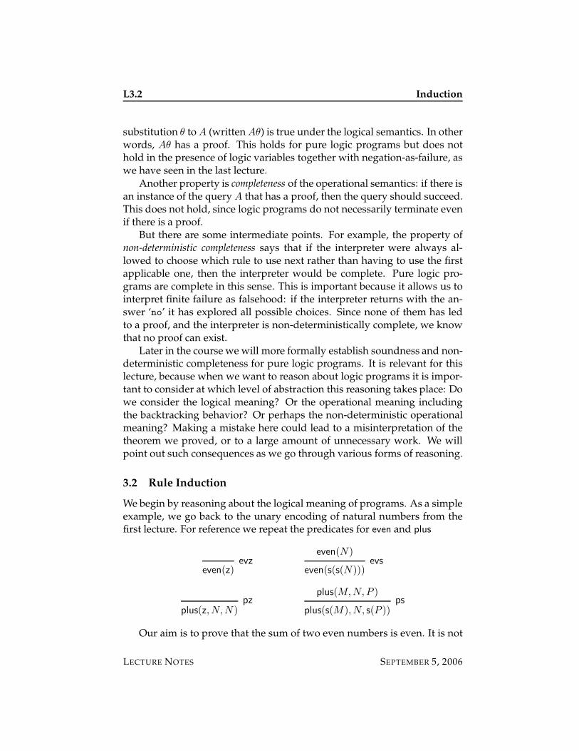
We begin by reasoning about the logical meaning of programs. As a simpleexample, we go back to the unary encoding of natural numbers from thefirst lecture. For reference we repeat the predicates for even and plus
even(z)evz
even(N)
even(s(s(N)))evs
plus(z, N,N)pz
plus(M,N,P )
plus(s(M),N, s(P ))ps
Our aim is to prove that the sum of two even numbers is even. It is not
LECTURE NOTES SEPTEMBER 5, 2006
Induction L3.3
immediately obvious how we can express this property on the relationalspecification. For example, we might say:
For any m, n, and p, if even(m) and even(n) and plus(m,n, p) theneven(p).
Or we could expressly require the existence of a sum p and the fact that itis even:
For any m, n, if even(m) and even(n) then there exists a p such thatplus(m,n, p) and even(p).
If we knew that plus is a total function in its first two arguments (that is,“For any m and n there exists a unique p such that plus(m,n, p).”), then thesetwo would be equivalent (see Exercise 3.2).
We will prove it in the second form. The first idea for this proof is usu-ally to examine the definition of plus and see that it is defined structurallyover its first argument m: the rule pz accounts for z and the rule ps reducess(m) to m. This suggests an induction over m. However, in the predicatecalculus (and therefore also in our logic programming language), m can bean arbitrary term and is therefore not a good candidate for induction.
Looking at the statement of the theorem, we see we are given the in-formation that even(m). This means that we have a deduction of even(m)using only the two rules evz and evs, since we viewed these two rules asa complete definition of the predicate even(m). This licenses us to proceedby induction on the structure of the deduction of even(m). This is some-times called rule induction. If we want to prove a property for all proofs of ajudgment, we consider each rule in turn. We may assume the property forall premisses of the rule and have to show that it holds for the conclusion.If we can show this for all rules, we know the property must hold for alldeductions.
In our proofs, we will need names for deductions. We use script lettersD, E , and so on, to denote deduction and use the two-dimensional notation
DJ
if D is a deduction of J .
Theorem 3.1 For any m, n, if even(m) and even(n) then there exists a p suchthat plus(m,n, p) and even(p).
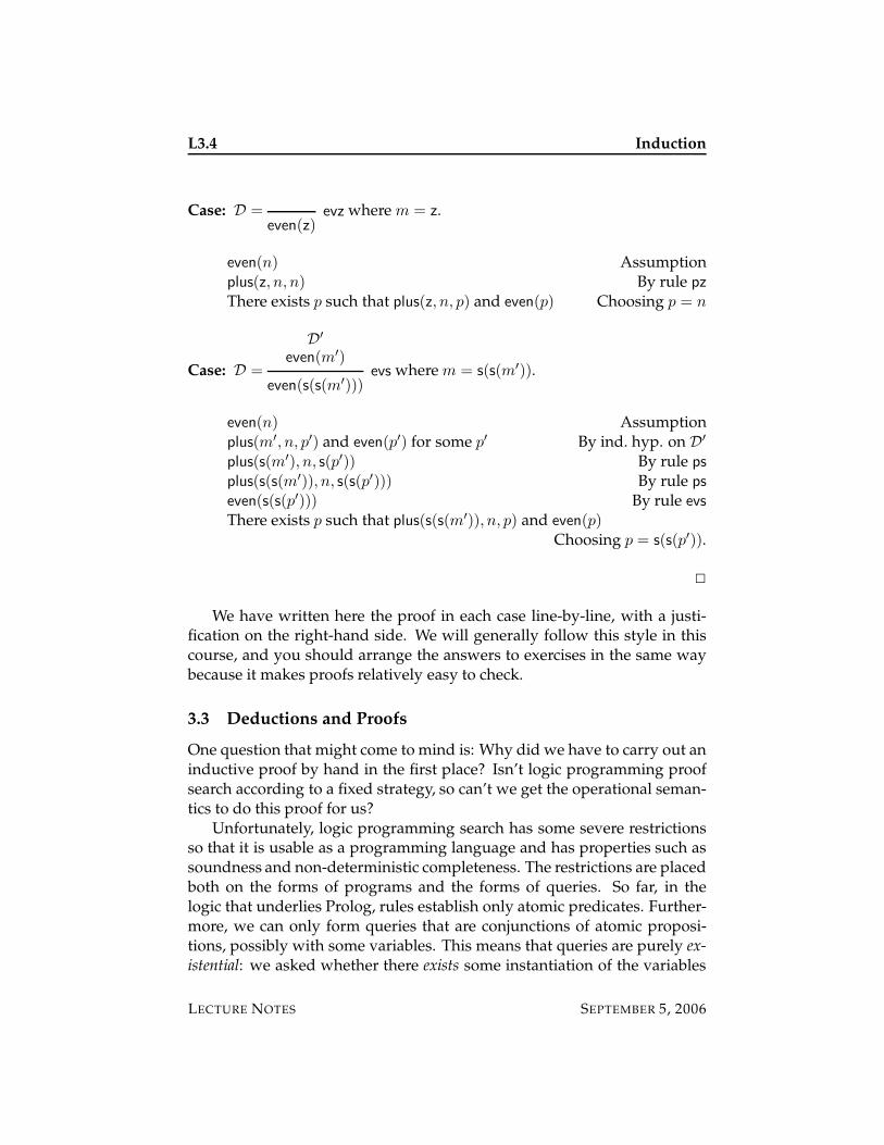
Proof: By induction on the structure of the deduction D of even(m).
LECTURE NOTES SEPTEMBER 5, 2006
L3.4 Induction
Case: D =even(z)
evz where m = z.
even(n) Assumptionplus(z, n, n) By rule pz
There exists p such that plus(z, n, p) and even(p) Choosing p = n
Case: D =
D′
even(m′)
even(s(s(m′)))evs where m = s(s(m′)).
even(n) Assumptionplus(m′, n, p′) and even(p′) for some p′ By ind. hyp. on D′
plus(s(m′), n, s(p′)) By rule ps
plus(s(s(m′)), n, s(s(p′))) By rule ps
even(s(s(p′))) By rule evs
There exists p such that plus(s(s(m′)), n, p) and even(p)Choosing p = s(s(p′)).
2
We have written here the proof in each case line-by-line, with a justi-fication on the right-hand side. We will generally follow this style in thiscourse, and you should arrange the answers to exercises in the same waybecause it makes proofs relatively easy to check.
3.3 Deductions and Proofs
One question that might come to mind is: Why did we have to carry out aninductive proof by hand in the first place? Isn’t logic programming proofsearch according to a fixed strategy, so can’t we get the operational seman-tics to do this proof for us?
Unfortunately, logic programming search has some severe restrictionsso that it is usable as a programming language and has properties such assoundness and non-deterministic completeness. The restrictions are placedboth on the forms of programs and the forms of queries. So far, in thelogic that underlies Prolog, rules establish only atomic predicates. Further-more, we can only form queries that are conjunctions of atomic proposi-tions, possibly with some variables. This means that queries are purely ex-istential: we asked whether there exists some instantiation of the variables
LECTURE NOTES SEPTEMBER 5, 2006
Induction L3.5
so that there exists a proof for the resulting proposition as in the query?- plus(s(z), s(s(z)), P) where we simultaneously ask for a p and aproof of plus(s(z), s(s(z)), p).
On the other hand, our theorem above is primarily universal and onlyon the inside do we see an existential quantifier: “For every m and n, and forevery deduction D of even(m) and E of even(n) there exists a p and deductions Fof plus(m,n, p) and G of even(p).”
This difference is also reflected in the structure of the proof. In responseto a logic programming query we only use the inference rules defining thepredicates directly. In the proof of the theorem about addition, we insteaduse induction in order to show that deductions of plus(m,n, p) and even(p)exist. If you carefully look at our proof, you will see that it contains a recipefor constructing these deductions from the given ones, but it does not con-struct them by backward search as in the operational semantics for logicprogramming. As we will see later in the course, it is in fact possible torepresent the induction proof of our first theorem also in logic program-ming, although it cannot be found only by logic programming search.
We will make a strict separation between proofs using only the infer-ence rules presented by the logic programmer and proofs about these rules.We will try to be consistent and write deduction for a proof constructed di-rectly with the rules and proof for an argument about the logical or opera-tional meaning of the rules. Similarly, we reserve the terms proposition, goal,and query for logic programs, and theorem for properties of logic programs.
3.4 Inversion
An important step in many induction proofs is inversion. The simplest formof inversion arises if have established that a certain proposition is true, andthat the proposition matches the conclusion of only one rule. In that casewe know that this rule must have been used, and that all premisses of therule must also be true. More generally, if the proposition matches the con-clusion of several rules, we can split the proof into cases, considering eachone in turn.
However, great care must be taken with applying inversion. In my ex-perience, the most frequent errors in proofs, both by students in coursessuch as this and in papers submitted to or even published in journals, are(a) missed cases that should have been considered, and (b) incorrect appli-cations of inversion. We can apply inversion only if we already know that ajudgment has a deduction, and then we have to take extreme care to makesure that we are indeed considering all cases.
LECTURE NOTES SEPTEMBER 5, 2006
L3.6 Induction
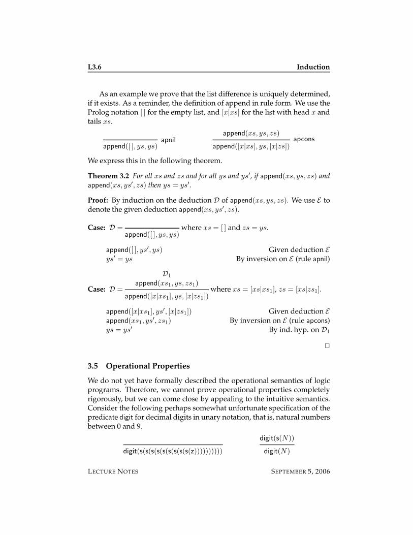
As an example we prove that the list difference is uniquely determined,if it exists. As a reminder, the definition of append in rule form. We use theProlog notation [ ] for the empty list, and [x|xs] for the list with head x andtails xs.
append([ ], ys, ys)apnil
append(xs, ys, zs)
append([x|xs], ys, [x|zs])apcons
We express this in the following theorem.
Theorem 3.2 For all xs and zs and for all ys and ys′, if append(xs, ys, zs) andappend(xs, ys′, zs) then ys = ys′.
Proof: By induction on the deduction D of append(xs, ys, zs). We use E todenote the given deduction append(xs, ys′, zs).
Case: D =append([ ], ys, ys)
where xs = [ ] and zs = ys.
append([ ], ys′, ys) Given deduction E
ys′ = ys By inversion on E (rule apnil)
Case: D =
D1
append(xs1, ys, zs1)
append([x|xs1], ys, [x|zs1])where xs = [xs|xs1], zs = [xs|zs1].
append([x|xs1], ys′, [x|zs1]) Given deduction E
append(xs1, ys′, zs1) By inversion on E (rule apcons)ys = ys′ By ind. hyp. on D1
2
3.5 Operational Properties
We do not yet have formally described the operational semantics of logicprograms. Therefore, we cannot prove operational properties completelyrigorously, but we can come close by appealing to the intuitive semantics.Consider the following perhaps somewhat unfortunate specification of thepredicate digit for decimal digits in unary notation, that is, natural numbersbetween 0 and 9.
digit(s(s(s(s(s(s(s(s(s(z))))))))))
digit(s(N))
digit(N)
LECTURE NOTES SEPTEMBER 5, 2006
Induction L3.7
For example, we can deduce that z is a digit by using the second rule ninetimes (working bottom up) and then closing of the deduction with the firstrule. In Prolog notation:
digit(s(s(s(s(s(s(s(s(s(z)))))))))).
digit(N) :- digit(s(N)).
While logically correct, this does not work correctly as a decision proce-dure, because it will not terminate for any argument greater than 9.
Theorem 3.3 Any query ?- digit(n) for n > 9 will not terminate.
Proof: By induction on the computation. If n > 9, then the first clausecannot apply. Therefore, the goal digit(n) must be reduced to the subgoaldigit(s(n)) by the second rule. But s(n) > 9 if n > 9, so by inductionhypothesis the subgoal will not terminate. Therefore the original goal alsodoes not terminate. 2
3.6 Aside: Forward Reasoning and Saturation
As mentioned in the first lecture, there is a completely different way tointerpret inference rules as logic programs than the reading that underliesProlog. This idea is to start with axioms (that is, inference rules with nopremisses) as logical truths and apply all rules in the forward direction,adding more true propositions. We stop when any rule application that wecould perform does not change the set of true propositions. In that casewe say the database of true propositions is saturated. In order to answer aquery we can now just look it up in the saturated database: if an instanceof the query is in the database, we succeed, otherwise we fail.
In the example from above, we start with a database consisting only ofdigit(s(s(s(s(s(s(s(s(s(z)))))))))). We can apply the second rule with this asa premiss to conclude that digit(s(s(s(s(s(s(s(s(z))))))))). We can repeat thisprocess a few more times until we finally conclude digit(z). At this point,any further rule applications would only add facts with already know: theset is saturated. We see that, consistent with the logical meaning, only thenumbers 0 through 9 are digits, other numbers are not.
In this example, the saturation-based operational semantics via forwardreasoning worked well for the given rules, while backward reasoning didnot. There are classes of algorithms which appear to be easy to describevia saturation, that appear significantly more difficult with backward rea-soning and vice versa. We will therefore return to forward reasoning and
LECTURE NOTES SEPTEMBER 5, 2006
L3.8 Induction
saturation later in the class, and also consider how it may be integratedwith backward reasoning in a logical way.
3.7 Historical Notes
The idea to mix reasoning about rules with the usual logic programmingsearch goes back to work by Eriksson and Hallnas [2] which led to theGCLA logic programming language [1]. However, it stops short of sup-porting full induction. More recently, this line of development been revivedby Tiu, Nadathur, and Miller [9]. Some of these ideas are embodied in theBedwyr system currently under development.
Another approach is to keep the layers separate, but provide meansto express proofs of properties of logic programs again as logic programs,as proposed by Schurmann [8]. These ideas are embodied in the Twelfsystem [6].
Saturating forward search has been the mainstay of the theorem prov-ing community since the pioneering work on resolution by Robinson [7].In logic programming, it has been called bottom-up evaluation and has his-torically been applied mostly in the context of databases [5] where satura-tion can often be guaranteed by language restrictions. Recently, it has beenrevisited as a tool for algorithm specification and complexity analysis byGanzinger and McAllester [3, 4].
3.8 Exercises
The proofs requested below should be given in the style presented in thesenotes, with careful justification for each step of reasoning. If you need alemma that has not yet been proven, carefully state and prove the lemma.
Exercise 3.1 Prove that the sum of two even numbers is even in the first formgiven in these notes.
Exercise 3.2 Prove that plus(m,n, p) is a total function of its first two argumentsand exploit this property to prove carefully that the two formulations of the prop-erty that the sum of two even numbers is even, are equivalent.
Exercise 3.3 Prove that times(m,n, p) is a total function of its first two argu-ments.
Exercise 3.4 Give a relational interpretation of the claim that “addition is com-mutative” and prove it.
LECTURE NOTES SEPTEMBER 5, 2006
Induction L3.9
Exercise 3.5 Prove that for any list xs, append(xs, [ ], xs).
Exercise 3.6 Give two alternative relational interpretations of the statement that“append is associative.” Prove one of them.
Exercise 3.7 Write a logic program to reverse a given list and prove that whenreversing the reversed list, we obtain the original list.
Exercise 3.8 Prove the correctness of quicksort from the previous lecture with re-spect to the specification from Exercise 2.2: If quicksort(xs, ys) is true thenthe second argument is an ordered permutation of the first. Your proof should bewith respect to logic programs to check whether a list is ordered, and whether onelist is a permutation of another.
3.9 References
[1] M. Aronsson, L.-H. Eriksson, A. Garedal, L. Hallnas, and P. Olin. Theprogramming language GCLA—a definitional approach to logic pro-gramming. New Generation Computing, 7(4):381–404, 1990.
[2] Lars-Henrik Eriksson and Lars Hallnas. A programming calculusbased on partial inductive definitions. SICS Research Report R88013,Swedish Institute of Computer Science, 1988.
[3] Harald Ganzinger and David A. McAllester. A new meta-complexitytheorem for bottom-up logic programs. In T.Nipkow R.Gore, A.Leitsch,editor, Proceedings of the First International Joint Conference on ArAuto-mated Reasoning (IJCAR’01), pages 514–528, Siena, Italy, June 2001.Springer-Verlag LNCS 2083.
[4] Harald Ganzinger and David A. McAllester. Logical algorithms. InP. Stuckey, editor, Proceedings of the 18th International Conference onLogic Programming, pages 209–223, Copenhagen, Denmark, July 2002.Springer-Verlag LNCS 2401.
[5] Jeff Naughton and Raghu Ramakrishnan. Bottom-up evaluation oflogic programs. In J.-L. Lassez and G. Plotkin, editors, ComputationalLogic. Essays in Honor of Alan Robinson, pages 640–700. MIT Press, Cam-bridge, Massachusetts, 1991.
[6] Frank Pfenning and Carsten Schurmann. System description: Twelf —a meta-logical framework for deductive systems. In H. Ganzinger, ed-itor, Proceedings of the 16th International Conference on Automated Deduc-tion (CADE-16), pages 202–206, Trento, Italy, July 1999. Springer-VerlagLNAI 1632.
LECTURE NOTES SEPTEMBER 5, 2006
L3.10 Induction
[7] J. A. Robinson. A machine-oriented logic based on the resolution prin-ciple. Journal of the ACM, 12(1):23–41, January 1965.
[8] Carsten Schurmann. Automating the Meta Theory of Deductive Systems.PhD thesis, Department of Computer Science, Carnegie Mellon Uni-versity, August 2000. Available as Technical Report CMU-CS-00-146.
[9] Alwen Tiu, Gopalan Nadathur, and Dale Miller. Mixing finite suc-cess and finite failure in an automated prover. In C.Benzmuller,J.Harrison, and C.Schurmann, editors, Proceedings of the Workshop onEmpirically Successful Automated Reasnoing in Higher-Order Logics (ES-HOL’05), pages 79–98, Montego Bay, Jamaica, December 2005.
LECTURE NOTES SEPTEMBER 5, 2006
15-819K: Logic Programming
Lecture 4
Operational Semantics
Frank Pfenning
September 7, 2006
In this lecture we begin in the quest to formally capture the operationalsemantics in order to prove properties of logic programs that depend on theway proof search proceeds. This will also allow us to relate the logical andoperational meaning of programs to understand deeper properties of logicprograms. It will also form the basis to prove the correctness of variousform of program analysis, such as type checking or termination checking,to be introduced later in the class.
4.1 Explicating Choices
To span the distance between the logical and the operational semantics wehave to explicate a series of choices that are fixed when proof search pro-ceeds. We will proceed in this order:
1. Left-to-right subgoal selection. In terms of inference rules, this meansthat we first search for a proof of the first premiss, then the second,etc.
2. First-to-last clause selection and backtracking. In terms of inferencerules this means when more than one rule is applicable, we begin bytrying the one listed first, then the one listed second, etc.
3. Unification. In terms of inference rules this means when we decidehow to instantiate the schematic variables in a rule and the unknownsin a goal, we use a particular algorithm to find the most general uni-fier between the conclusion of the rule and the goal.
LECTURE NOTES SEPTEMBER 7, 2006
L4.2 Operational Semantics
4. Cut. This has no reflection at the level of inference rules. We have tospecify how we commit to particular choices made so far when weencounter a cut or another control constructs such as a conditional.
5. Other built-in predicates. Prolog has other built-in predicates forarithmetic, input and output, changing the program at run-time, for-eign function calls, and more which we will not treat formally.
It is useful not to jump directly to the most accurate and low-level se-mantics, because we often would like to reason about properties of pro-grams that are independent of such detail. One set of examples we havealready seen: we can reason about the logical semantics to establish prop-erties such as that the sum of two even numbers is even. In that case we areonly interested in successful computations, and how we searched for themis not important. Another example is represented by cut: if a program doesnot contain any cuts, the complexity of the semantics that captures it is un-warranted.
4.2 Definitional Intpreters
The general methodology we follow goes back to Reynolds [3], adaptedhere to logic programming. We can write an interpreter for a languagein the language itself (or a very similar language), a so-called definitionalinterpreter, meta-interpreter, or meta-circular interpreter. This may fail to com-pletely determine the behavior of the language we are studying (the objectlanguage), because it may depend on the behavior of the language in whichwe write the definition (the meta-language), and the two are the same! Wethen transform the definitional interpreter, removing some of the advancedfeatures of the language we are defining, so that now the more advancedconstructs are explained in terms of simpler ones, removing circular as-pects. We can interate the process until we arrive at the desired level ofspecification.
For Prolog (although not pure first-order logic programming), the sim-plest meta-interpreter, hardly deserving the name, is
solve(A) :- A.
To interpret the argument to solve as a goal, we simply execute it using themeta-call facility of Prolog.
This does not provide a lot of insight, but it brings up the first issue:how do we represent logic programs and goals in order to execute them
LECTURE NOTES SEPTEMBER 7, 2006
Operational Semantics L4.3
in our definitional interpreter? In Prolog, the answer is easy: we think ofthe comma which separates the subgoal of a clause as a binary functionsymbol denoting conjunction, and we think of the constant true which al-ways succeeds as just a constant. One can think of this as replicating thelanguage of predicates in the language of function symbols, or not distin-guishing between the two. The code above, if it were formally justifiedusing higher-order logic, would take the latter approach: logical connec-tives are data and can be treated as such. In the next interpreter we takethe first approach: we overload comma to separate subgoals in the meta-language, but we also use it as a function symbol to describe conjunctionin the object language. Unlike in the code above, we will not mix the two.The logical constant true is similarly overloaded as a predicate constant ofthe same name.
solve(true).
solve((A , B)) :- solve(A), solve(B).
solve(P) :- clause(P, B), solve(B).
In the second clause, the head solve((A , B)) employs infix notation,and could be written equivalently as solve(’,’(A, B)).1 The additionalpair of parentheses is necessary since solve(A , B) would be incorrectlyseen as a predicate solve with two arguments.
The predicate clause/2 is a built-in predicate of Prolog.2 The subgoalclause(P, B) will unify P with the head of each program clause and B
with the corresponding body. In other words, if clause(P, B) succeeds,then P :- B. is an instance of a clause in the current program. Prolog willtry to unify P and B with the clauses of the current program first-to-last,so that the above meta-interpreter will work correctly with respect to theintuitive semantics explained earlier.
There is a small amount of standardization in that a clause P. in theprogram with an empty body is treated as if it were P :- true.
This first interpreter does not really explicate anything: the order inwhich subgoals are solved in the object language is the same as the orderin the meta-language, according to the second clause. The order in whichclauses are tried is the order in which clause/2 delivers them. And unifi-cation between the goal and the clause head is also inherited by the object
1In Prolog, we can quote an infix operator to use it as an ordinary function or predicatesymbol.
2In Prolog, it is customary to write p/n when refering to a predicate p of arity n, sincemany predicates have different meanings at different arities.
LECTURE NOTES SEPTEMBER 7, 2006
L4.4 Operational Semantics
language from the meta-language through the unification carried out byclause(P, B) between its first argument and the clause heads in the pro-gram.
4.3 Subgoal Order
According to our outline, the first task is to modify our interpreter so thatthe order in which subgoals are solved is made explicit. When encounter-ing a goal (A , B) we push B onto a stack and solve A first. When A ashas been solved we then pop B off the stack and solve it. We could repre-sent the stack as a list, but we find it somewhat more elegant to representthe goal stack itself as a conjunction of goals because all the elements ofgoal stack have to be solved for the overall goal to succeed.
The solve predicate now takes two arguments, solve(A, S) where A
is the goal, and S is a stack of yet unsolved goals. We start with the emptystack, represented by true.
solve(true, true).
solve(true, (A , S)) :- solve(A, S).
solve((A , B), S) :- solve(A, (B , S)).
solve(P, S) :- clause(P, B), solve(B, S).
We explain each clause in turn.If the goal is solved and the goal stack is empty, we just succeed.
solve(true, true).
If the goal is solved and the goal stack is non-empty, we pop the mostrecent subgoal A of the stack and solve it.
solve(true, (A , S)) :- solve(A, S).
If the goal is a conjunction, we solve the first conjunct, pushing the sec-ond one on the goal stack.
solve((A , B), S) :- solve(A, (B , S)).
When the goal is atomic, we match it against the heads of all clauses inturn, solving the body of the clause as a subgoal.
solve(P, S) :- clause(P, B), solve(B, S).
We do not explicitly check that P is atomic, because clause(P, B) willfail if it is not.
LECTURE NOTES SEPTEMBER 7, 2006
Operational Semantics L4.5
4.4 Subgoal Order More Abstractly
The interpreter from above works for pure Prolog as intended. Now wewould like to prove properties of it, such as its soundness: if it provessolve(A, true) then it is indeed the case that A is true. In order to dothat it is advisable to reconstruct the interpreter above in logical form, sowe can use induction on the structure of deductions in a rigorous manner.
The first step is to define our first logical connective: conjunction! Wealso need a propositional constant denoting truth. It is remarkable thatfor all the development of logic programming so far, not a single logicalconnective was needed, just atomic propositions, the truth judgment, anddeductions as evidence for truth.
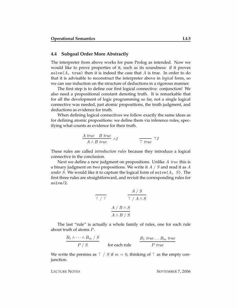
When defining logical connectives we follow exactly the same ideas asfor defining atomic propositions: we define them via inference rules, spec-ifying what counts as evidence for their truth.
A true B true
A ∧ B true∧I
> true>I
These rules are called introduction rules because they introduce a logicalconnective in the conclusion.
Next we define a new judgment on propositions. Unlike A true this isa binary judgment on two propositions. We write it A / S and read it as A
under S. We would like it to capture the logical form of solve(A, S). Thefirst three rules are straightforward, and revisit the corresponding rules forsolve/2.
> / >
A / S
> / A ∧ S
A / B ∧ S
A ∧ B / S
The last “rule” is actually a whole family of rules, one for each ruleabout truth of atoms P .
B1 ∧ · · · ∧ Bm / S
P / S for each rule
B1 true . . . Bm true
P true
We write the premiss as > / S if m = 0, thinking of > as the empty con-junction.
LECTURE NOTES SEPTEMBER 7, 2006
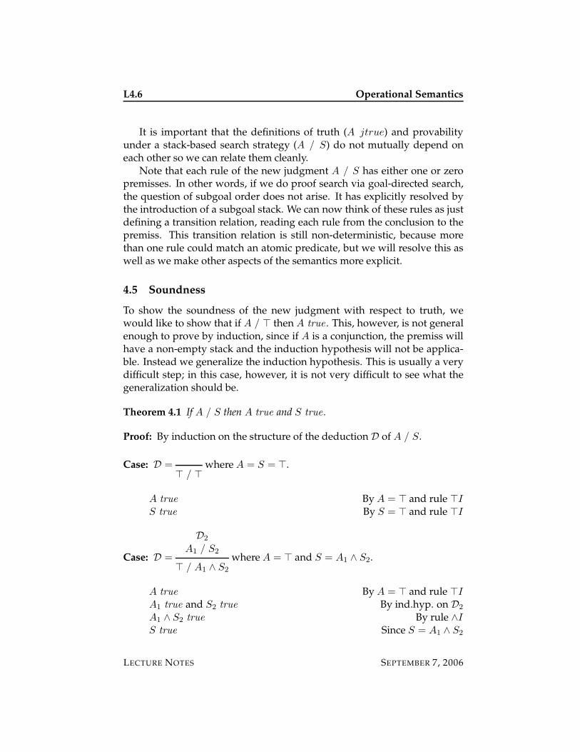
L4.6 Operational Semantics
It is important that the definitions of truth (A jtrue) and provabilityunder a stack-based search strategy (A / S) do not mutually depend oneach other so we can relate them cleanly.
Note that each rule of the new judgment A / S has either one or zeropremisses. In other words, if we do proof search via goal-directed search,the question of subgoal order does not arise. It has explicitly resolved bythe introduction of a subgoal stack. We can now think of these rules as justdefining a transition relation, reading each rule from the conclusion to thepremiss. This transition relation is still non-deterministic, because morethan one rule could match an atomic predicate, but we will resolve this aswell as we make other aspects of the semantics more explicit.
4.5 Soundness
To show the soundness of the new judgment with respect to truth, wewould like to show that if A / > then A true . This, however, is not generalenough to prove by induction, since if A is a conjunction, the premiss willhave a non-empty stack and the induction hypothesis will not be applica-ble. Instead we generalize the induction hypothesis. This is usually a verydifficult step; in this case, however, it is not very difficult to see what thegeneralization should be.
Theorem 4.1 If A / S then A true and S true .
Proof: By induction on the structure of the deduction D of A / S.
Case: D => / >
where A = S = >.
A true By A = > and rule >I
S true By S = > and rule >I
Case: D =
D2
A1 / S2
> / A1 ∧ S2
where A = > and S = A1 ∧ S2.
A true By A = > and rule >I
A1 true and S2 true By ind.hyp. on D2
A1 ∧ S2 true By rule ∧I
S true Since S = A1 ∧ S2
LECTURE NOTES SEPTEMBER 7, 2006
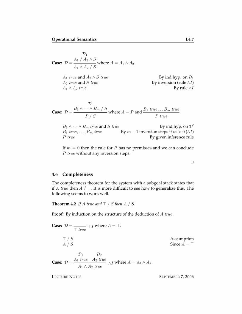
Operational Semantics L4.7
Case: D =
D1
A1 / A2 ∧ S
A1 ∧ A2 / Swhere A = A1 ∧ A2.
A1 true and A2 ∧ S true By ind.hyp. on D1
A2 true and S true By inversion (rule ∧I)A1 ∧ A2 true By rule ∧I
Case: D =
D′
B1 ∧ · · · ∧ Bm / S
P / Swhere A = P and
B1 true . . . Bm true
P true.
B1 ∧ · · · ∧ Bm true and S true By ind.hyp. on D′
B1 true, . . . , Bm true By m − 1 inversion steps if m > 0 (∧I)P true By given inference rule
If m = 0 then the rule for P has no premisses and we can concludeP true without any inversion steps.
2
4.6 Completeness
The completeness theorem for the system with a subgoal stack states thatif A true then A / >. It is more difficult to see how to generalize this. Thefollowing seems to work well.
Theorem 4.2 If A true and > / S then A / S.
Proof: By induction on the structure of the deduction of A true .
Case: D => true
>I where A = >.
> / S AssumptionA / S Since A = >
Case: D =
D1
A1 true
D2
A2 true
A1 ∧ A2 true∧I where A = A1 ∧ A2.
LECTURE NOTES SEPTEMBER 7, 2006
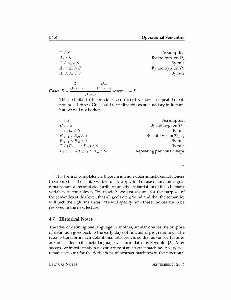
L4.8 Operational Semantics
> / S AssumptionA2 / S By ind.hyp. on D2
> / A2 ∧ S By ruleA1 / A2 ∧ S By ind.hyp. on D1
A1 ∧ A2 / S By rule
Case: D =
D1
B1 true . . .
Dm
Bm true
P truewhere A = P .
This is similar to the previous case, except we have to repeat the pat-tern m − 1 times. One could formalize this as an auxiliary induction,but we will not bother.
> / S AssumptionBm / S By ind.hyp. on Dm
> / Bm ∧ S By ruleBm−1 / Bm ∧ S By ind.hyp. on Dm−1
Bm−1 ∧ Bm / S By rule> / (Bm−1 ∧ Bm) ∧ S By ruleB1 ∧ . . . ∧ Bm−1 ∧ Bm / S Repeating previous 3 steps
2
This form of completeness theorem is a non-deterministic completenesstheorem, since the choice which rule to apply in the case of an atomic goalremains non-deterministic. Furthermore, the instantiation of the schematicvariables in the rules is “by magic”: we just assume for the purpose ofthe semantics at this level, that all goals are ground and that the semanticswill pick the right instances. We will specify how these choices are to beresolved in the next lecture.
4.7 Historical Notes
The idea of defining one language in another, similar one for the purposeof definition goes back to the early days of functional programming. Theidea to transform such definitional interpreters so that advanced featuresare not needed in the meta-language was formulated by Reynolds [3]. Aftersuccessive transformation we can arrive at an abstract machine. A very sys-tematic account for the derivations of abstract machines in the functional
LECTURE NOTES SEPTEMBER 7, 2006
Operational Semantics L4.9
setting has been given by Danvy and several of his students (see, for exam-ple, [1]). Meta-interpreters are also common in logic programming, mostlywith the goal to extend capabilities of the language. One of the earliestpublished account is by Bowen and Kowalski [2].
4.8 Exercises
Exercise 4.1 Extend the meta-interpreter without goal stacks to a bounded inter-preter which fails if no proof of a given depth can be found. In terms of proof trees,the depth is length of the longest path from the final conclusion to an axiom.
Exercise 4.2 Extend the meta-interpreter without goal stacks with loop detection,so that if while solving an atomic goal P the identical goal P arises again, thatbranch of the search will be terminated with failure instead of diverging. You mayassume that all goals are ground.
Exercise 4.3 Extend the meta-interpreter with goal stacks so that if an atomic goalsucceeds once, we do not search for a proof of it again but just succeed. You mayassume that all goals are ground and you do not need to preserve the memo tableupon backtracking.
Exercise 4.4 Extend the meta-interpreter with the goal stack to trace the executionof a program, printing information about the state of search.
4.9 References
[1] Mads Sig Ager, Dariusz Biernacki, Olivier Danvy, and Jan Midtgaard.A functional correspondence between evluators and abstract machines.In Proceedings of the 5th International Conference on Principles and Practiceof Declarative Programming (PPDP’03), pages 8–19, Uppsala, Sweden,August 2003. ACM Press.
[2] Kenneth A. Bowen and Robert A. Kowalski. Amalgamating languageand metalanguage in logic programming. In K.L. Clark and S.-A.Tarnlund, editors, Logic Programming, pages 153–172. Academic Press,London, 1982.
[3] John C. Reynolds. Definitional interpreters for higher-order program-ming languages. In Proceedings of the ACM Annual Conference, pages717–740, Boston, Massachusetts, August 1972. ACM Press. Reprintedin Higher-Order and Symbolic Computation, 11(4), pp.363–397, 1998.
LECTURE NOTES SEPTEMBER 7, 2006

L4.10 Operational Semantics
LECTURE NOTES SEPTEMBER 7, 2006
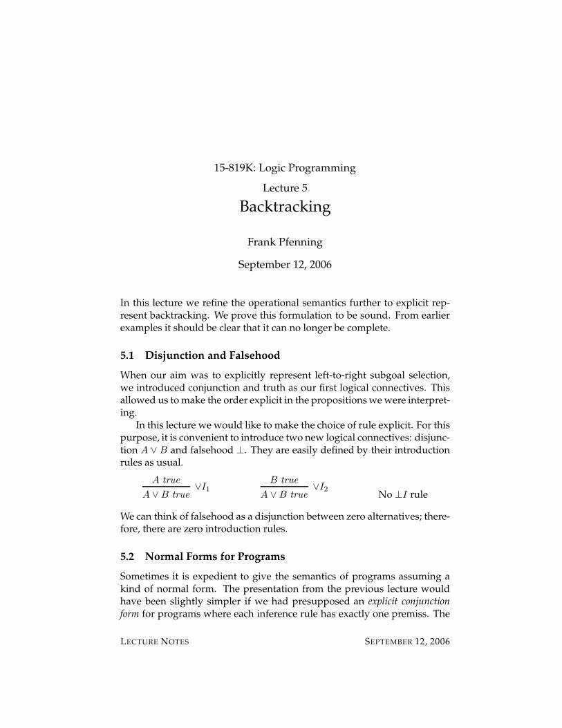
15-819K: Logic Programming
Lecture 5
Backtracking
Frank Pfenning
September 12, 2006
In this lecture we refine the operational semantics further to explicit rep-resent backtracking. We prove this formulation to be sound. From earlierexamples it should be clear that it can no longer be complete.
5.1 Disjunction and Falsehood
When our aim was to explicitly represent left-to-right subgoal selection,we introduced conjunction and truth as our first logical connectives. Thisallowed us to make the order explicit in the propositions we were interpret-ing.
In this lecture we would like to make the choice of rule explicit. For thispurpose, it is convenient to introduce two new logical connectives: disjunc-tion A ∨ B and falsehood ⊥. They are easily defined by their introductionrules as usual.
A true
A ∨ B true∨I1
B true
A ∨ B true∨I2
No ⊥I rule
We can think of falsehood as a disjunction between zero alternatives; there-fore, there are zero introduction rules.
5.2 Normal Forms for Programs
Sometimes it is expedient to give the semantics of programs assuming akind of normal form. The presentation from the previous lecture wouldhave been slightly simpler if we had presupposed an explicit conjunctionform for programs where each inference rule has exactly one premiss. The
LECTURE NOTES SEPTEMBER 12, 2006
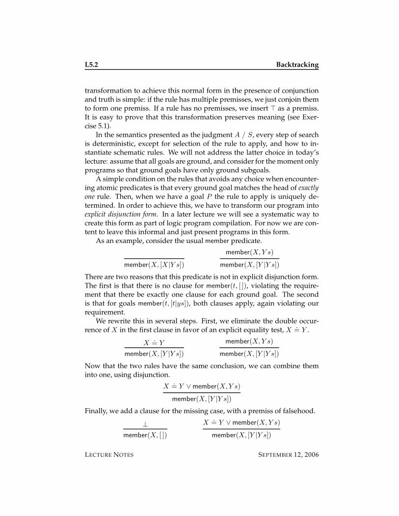
L5.2 Backtracking
transformation to achieve this normal form in the presence of conjunctionand truth is simple: if the rule has multiple premisses, we just conjoin themto form one premiss. If a rule has no premisses, we insert > as a premiss.It is easy to prove that this transformation preserves meaning (see Exer-cise 5.1).
In the semantics presented as the judgment A / S, every step of searchis deterministic, except for selection of the rule to apply, and how to in-stantiate schematic rules. We will not address the latter choice in today’slecture: assume that all goals are ground, and consider for the moment onlyprograms so that ground goals have only ground subgoals.
A simple condition on the rules that avoids any choice when encounter-ing atomic predicates is that every ground goal matches the head of exactlyone rule. Then, when we have a goal P the rule to apply is uniquely de-termined. In order to achieve this, we have to transform our program intoexplicit disjunction form. In a later lecture we will see a systematic way tocreate this form as part of logic program compilation. For now we are con-tent to leave this informal and just present programs in this form.
As an example, consider the usual member predicate.
member(X, [X|Y s])
member(X,Y s)
member(X, [Y |Y s])
There are two reasons that this predicate is not in explicit disjunction form.The first is that there is no clause for member(t, [ ]), violating the require-ment that there be exactly one clause for each ground goal. The secondis that for goals member(t, [t|ys]), both clauses apply, again violating ourrequirement.
We rewrite this in several steps. First, we eliminate the double occur-rence of X in the first clause in favor of an explicit equality test, X
.= Y .
X.= Y
member(X, [Y |Y s])
member(X,Y s)
member(X, [Y |Y s])
Now that the two rules have the same conclusion, we can combine theminto one, using disjunction.
X.= Y ∨ member(X,Y s)
member(X, [Y |Y s])
Finally, we add a clause for the missing case, with a premiss of falsehood.
⊥
member(X, [ ])
X.= Y ∨ member(X,Y s)
member(X, [Y |Y s])
LECTURE NOTES SEPTEMBER 12, 2006
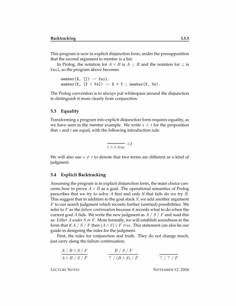
Backtracking L5.3
This program is now in explicit disjunction form, under the presuppositionthat the second argument to member is a list.
In Prolog, the notation for A ∨ B is A ; B and the notation for ⊥ isfail, so the program above becomes
member(X, []) :- fail.
member(X, [Y | Ys]) :- X = Y ; member(X, Ys).
The Prolog convention is to always put whitespace around the disjunctionto distinguish it more clearly from conjunction.
5.3 Equality
Transforming a program into explicit disjunction form requires equality, aswe have seen in the member example. We write s
.= t for the proposition
that s and t are equal, with the following introduction rule.
t.= t true
.=I
We will also use s 6= t to denote that two terms are different as a kind ofjudgment.
5.4 Explicit Backtracking
Assuming the program is in explicit disjunction form, the main choice con-cerns how to prove A ∨ B as a goal. The operational semantics of Prologprescribes that we try to solve A first and only if that fails do we try B.This suggest that in addition to the goal stack S, we add another argumentF to our search judgment which records further (untried) possibilities. Werefer to F as the failure continuation because it records what to do when thecurrent goal A fails. We write the new judgment as A / S / F and read thisas: Either A under S or F . More formally, we will establish soundness in theform that if A / S / F then (A∧S)∨F true . This statement can also be ourguide in designing the rules for the judgment.
First, the rules for conjunction and truth. They do not change much,just carry along the failure continuation.
A / B ∧ S / F
A ∧ B / S / F
B / S / F
> / (B ∧ S) / F > / > / F
LECTURE NOTES SEPTEMBER 12, 2006
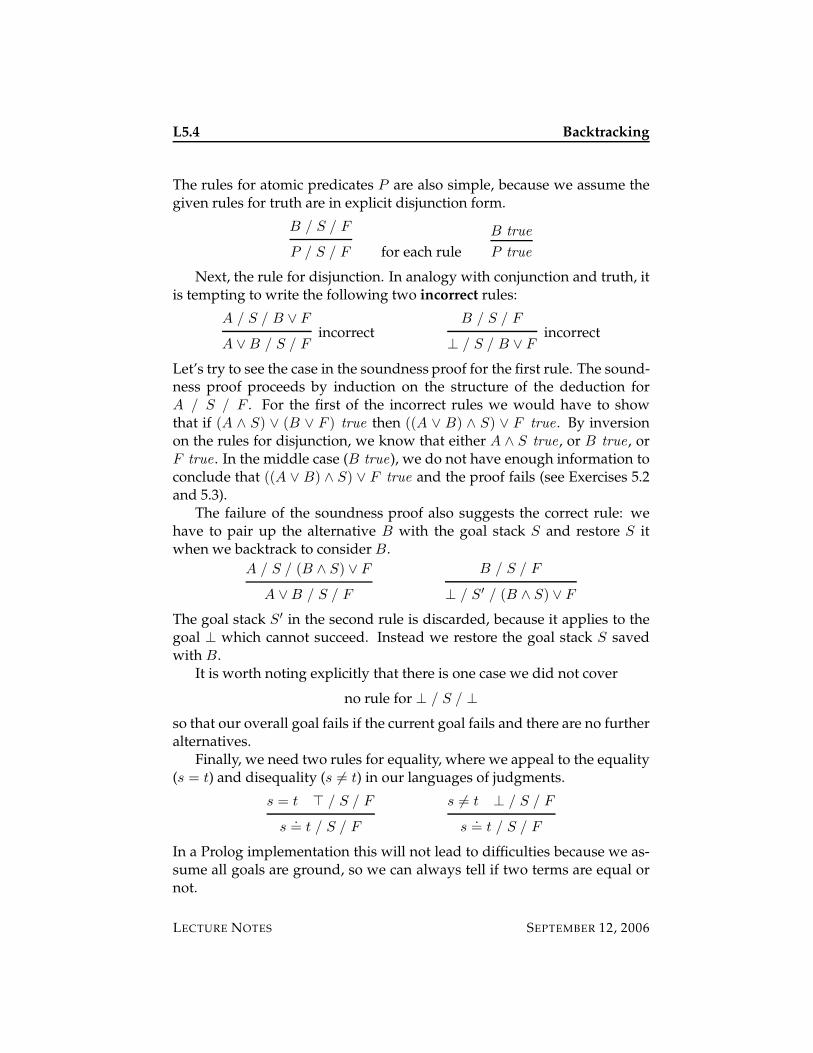
L5.4 Backtracking
The rules for atomic predicates P are also simple, because we assume thegiven rules for truth are in explicit disjunction form.
B / S / F
P / S / F for each rule
B true
P true
Next, the rule for disjunction. In analogy with conjunction and truth, itis tempting to write the following two incorrect rules:
A / S / B ∨ F
A ∨ B / S / Fincorrect
B / S / F
⊥ / S / B ∨ Fincorrect
Let’s try to see the case in the soundness proof for the first rule. The sound-ness proof proceeds by induction on the structure of the deduction forA / S / F . For the first of the incorrect rules we would have to showthat if (A ∧ S) ∨ (B ∨ F ) true then ((A ∨ B) ∧ S) ∨ F true . By inversionon the rules for disjunction, we know that either A ∧ S true , or B true , orF true . In the middle case (B true), we do not have enough information toconclude that ((A ∨ B) ∧ S) ∨ F true and the proof fails (see Exercises 5.2and 5.3).
The failure of the soundness proof also suggests the correct rule: wehave to pair up the alternative B with the goal stack S and restore S itwhen we backtrack to consider B.
A / S / (B ∧ S) ∨ F
A ∨ B / S / F
B / S / F
⊥ / S′ / (B ∧ S) ∨ F
The goal stack S′ in the second rule is discarded, because it applies to thegoal ⊥ which cannot succeed. Instead we restore the goal stack S savedwith B.
It is worth noting explicitly that there is one case we did not cover
no rule for ⊥ / S / ⊥
so that our overall goal fails if the current goal fails and there are no furtheralternatives.
Finally, we need two rules for equality, where we appeal to the equality(s = t) and disequality (s 6= t) in our languages of judgments.
s = t > / S / F
s.= t / S / F
s 6= t ⊥ / S / F
s.= t / S / F
In a Prolog implementation this will not lead to difficulties because we as-sume all goals are ground, so we can always tell if two terms are equal ornot.
LECTURE NOTES SEPTEMBER 12, 2006
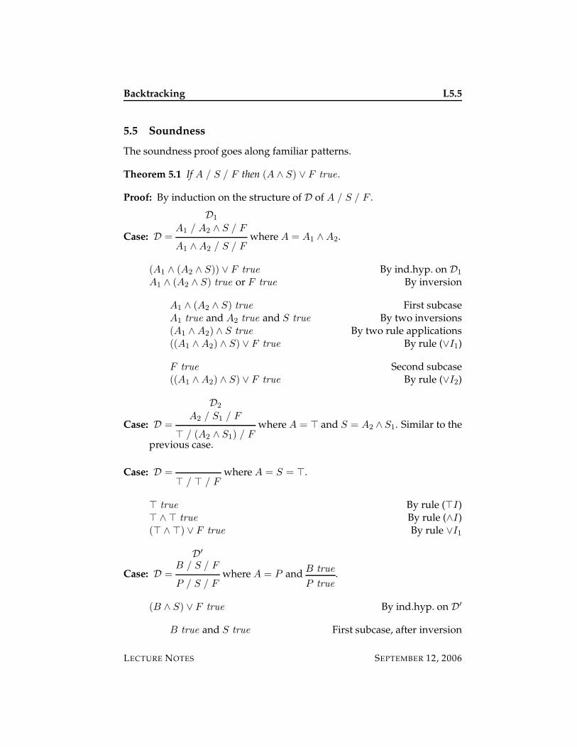
Backtracking L5.5
5.5 Soundness
The soundness proof goes along familiar patterns.
Theorem 5.1 If A / S / F then (A ∧ S) ∨ F true .
Proof: By induction on the structure of D of A / S / F .
Case: D =
D1
A1 / A2 ∧ S / F
A1 ∧ A2 / S / Fwhere A = A1 ∧ A2.
(A1 ∧ (A2 ∧ S)) ∨ F true By ind.hyp. on D1
A1 ∧ (A2 ∧ S) true or F true By inversion
A1 ∧ (A2 ∧ S) true First subcaseA1 true and A2 true and S true By two inversions(A1 ∧ A2) ∧ S true By two rule applications((A1 ∧ A2) ∧ S) ∨ F true By rule (∨I1)
F true Second subcase((A1 ∧ A2) ∧ S) ∨ F true By rule (∨I2)
Case: D =
D2
A2 / S1 / F
> / (A2 ∧ S1) / Fwhere A = > and S = A2 ∧ S1. Similar to the
previous case.
Case: D => / > / F
where A = S = >.
> true By rule (>I)> ∧> true By rule (∧I)(> ∧>) ∨ F true By rule ∨I1
Case: D =
D′
B / S / F
P / S / Fwhere A = P and
B true
P true.
(B ∧ S) ∨ F true By ind.hyp. on D′
B true and S true First subcase, after inversion
LECTURE NOTES SEPTEMBER 12, 2006
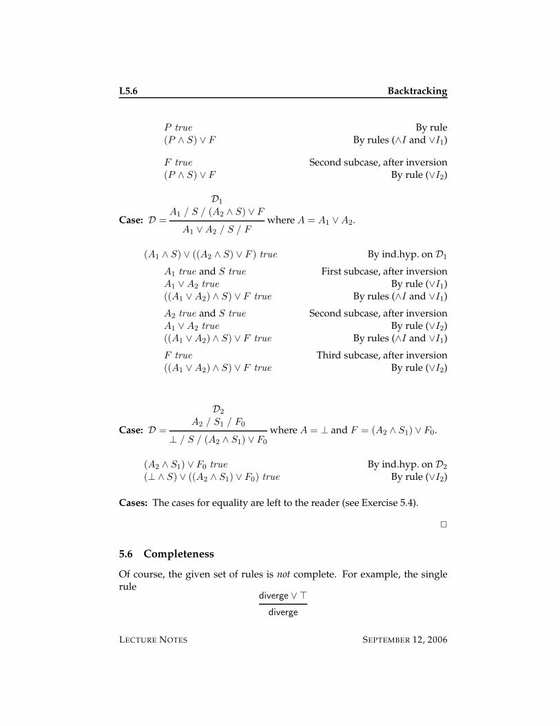
L5.6 Backtracking
P true By rule(P ∧ S) ∨ F By rules (∧I and ∨I1)
F true Second subcase, after inversion(P ∧ S) ∨ F By rule (∨I2)
Case: D =
D1
A1 / S / (A2 ∧ S) ∨ F
A1 ∨ A2 / S / Fwhere A = A1 ∨ A2.
(A1 ∧ S) ∨ ((A2 ∧ S) ∨ F ) true By ind.hyp. on D1
A1 true and S true First subcase, after inversionA1 ∨ A2 true By rule (∨I1)((A1 ∨ A2) ∧ S) ∨ F true By rules (∧I and ∨I1)
A2 true and S true Second subcase, after inversionA1 ∨ A2 true By rule (∨I2)((A1 ∨ A2) ∧ S) ∨ F true By rules (∧I and ∨I1)
F true Third subcase, after inversion((A1 ∨ A2) ∧ S) ∨ F true By rule (∨I2)
Case: D =
D2
A2 / S1 / F0
⊥ / S / (A2 ∧ S1) ∨ F0
where A = ⊥ and F = (A2 ∧ S1) ∨ F0.
(A2 ∧ S1) ∨ F0 true By ind.hyp. on D2
(⊥ ∧ S) ∨ ((A2 ∧ S1) ∨ F0) true By rule (∨I2)
Cases: The cases for equality are left to the reader (see Exercise 5.4).
2
5.6 Completeness
Of course, the given set of rules is not complete. For example, the singlerule
diverge ∨ >
diverge
LECTURE NOTES SEPTEMBER 12, 2006
Backtracking L5.7
cannot be found by search, that is, there is no proof of
diverge / > / ⊥
even though there is a simple proof that diverge true .
> true>I
diverge ∨ > true∨I2
diverge true
However, it is interesting to consider that the set of rules is complete aweaker sense, namely that if A / > / ⊥ can be reduced to ⊥ / S / ⊥ thenthere can be no proof of A true . We will not do this here (see Exercise 5.5).One way to approach this formally is to add another argument and use afour-place judgment
A / S / F / J
where J is either istrue (if a proof can be found) or isfalse (if the the attemptto find a proof fails finitely).
5.7 A Meta-Interpreter with Explicit Backtracking
Based on the idea at the end of the last section, we can turn the inferencesystem into a Prolog program that can tell us explicitly whenever searchsucceeds or fails finitely.
Recall the important assumption that all goals are ground, and that theprogram is in explicit disjunction form.
solve(true, true, _, istrue).
solve(true, (A , S), F, J) :- solve(A, S, F, J).
solve((A , B), S, F, J) :- solve(A, (B, S), F, J).
solve(fail, _, fail, isfalse).
solve(fail, _, ((B , S) ; F), J) :- solve(B, S, F, J).
solve((A ; B), S, F, J) :- solve(A, S, ((B , S) ; F), J).
solve((X = Y), S, F, J) :- X = Y, solve(true, S, F, J).
solve((X = Y), S, F, J) :- X \= Y, solve(fail, S, F, J).
solve(P, S, F, J) :- clause(P, B), solve(B, S, F, J).
% top level interface
solve(A, J) :- solve(A, true, fail, J).
LECTURE NOTES SEPTEMBER 12, 2006
L5.8 Backtracking
Given a program in explicit disjunction form, such as
member(X, []) :- fail.
member(X, [Y|Ys]) :- X = Y ; member(X, Ys).
we can now ask
?- solve(member(1, [2,3,4]), J).
J = isfalse;
?- solve(member(1, [1,2,1,4]), J).
J = istrue;
Each query will succeed only once since our meta-interpreter only searchesfor the first solution (see Exercise 5.6).
5.8 Abstract Machines
The meta-interpreter in which both subgoal selection and backtracking areexplicit comes close to the specification of an abstract machine. In orderto see how the inference rule can be seen as transition rules, we considerA / S / F as the state of the machine. Each rule for this judgment has onlyone premiss, so each rule, when read from the conclusion to the premisscan be seen as a transition rule for an abstract machine.
Examining the rules we can see that for every state there is a uniquestate transition, with the following exceptions:
1. A state > / > / F is final since there is no premiss for the machingrule. The computation finishes.
2. A state ⊥ / S / ⊥ is final since there is no rule that applies. Thecomputation fails.
3. A state P / S / F applies a unique transition (by the requirement thatthere be a unique rule for every atomic goal P ), although how to findthat rule instance remains informal.
In the next lecture we make the process of rule application more precise,and we also admit goals with free variables as in Prolog.
LECTURE NOTES SEPTEMBER 12, 2006
Backtracking L5.9
5.9 Historical Notes
The explicit disjunction form is a pre-cursor of Clark’s iff-completion of aprogram [2]. This idea is quite general, is useful in compilation of logicprograms, and can be applied to much richer logic programming languagesthan Horn logic [1].
Early logic programming theory generally did not make backtrackingexplicit. Some references will appear in the next lecture, since some of theintrinsic interest arises from the notion of substitution and unification.
5.10 Exercises
Exercise 5.1 Prove that if we replace every rule
B1 true . . . Bm true
P true
byB1 ∧ · · · ∧ Bm true
P true
to achieve the explicit conjunction form, the original and revised specificationare strongly equivalent in the sense that there is a bijection between the proofsin the two formulations for each atomic proposition. Read the empty conjunction(m = 0) as >.
Exercise 5.2 Give a counterexample to show that the failure in the soundnessproof for the first incorrect disjunction rule is not just a failure in the proof: thesystem is actually unsound with respect to logical truth.
Exercise 5.3 Investigate if the second incorrect rule for disjunction
B / S / F
⊥ / S / B ∨ Fincorrect
also leads to a failure in the soundness proof. If so, give a counterexample. If not,discuss in what sense this rule is nonetheless incorrect.
Exercise 5.4 Complete the soundness proof by giving the cases for equality.
Exercise 5.5 Investigate weaker notions of completeness for the backtracking se-mantics, as mentioned at the end of the section of completeness.
LECTURE NOTES SEPTEMBER 12, 2006
L5.10 Backtracking
Exercise 5.6 Rewrite the meta-interpreter so it counts the number of proofs of agoal instead of returning just an indication of whether it is true or false. You maymake all the same assumptions that solve(A, S, F, J) makes.
Exercise 5.7 Revisit the example from Lecture 3
digit(s(s(s(s(s(s(s(s(s(z))))))))))
digit(s(N))
digit(N)
and prove more formally now that any query ?- digit(n) for n > 9 will notterminate. You should begin by rewriting the program into explicit disjunctionform. Please be clear what you are doing the induction over (if you use induction),and explain in which way your theorem captures the statement above.
Exercise 5.8 If we were not concerned about space usage or efficiency, we couldwrite a breadth-first interpreter instead of backtracking. Specify such an inter-preter using the judgmental style and prove that it is sound and complete withrespect to logical truth. Translate your interpreter into a Prolog program.
5.11 References
[1] Iliano Cervesato. Proof-theoretic foundation of compilation in logicprogramming languages. In J. Jaffar, editor, Proceedings of the Joint In-ternational Conference and Symposium on Logic Programming (JICSLP’98),pages 115–129, Manchester, England, June 1998. MIT Press.
[2] Keith L. Clark. Negation as failure. In H. Gallaire and J. Minker, edi-tors, Logic and Databases, pages 293–322. Plenum Press, New York, 1978.
LECTURE NOTES SEPTEMBER 12, 2006
15-819K: Logic Programming
Lecture 6
Unification
Frank Pfenning
September 14, 2006
In this lecture we take the essential step towards making the choice of goaland rule instantiation explicit in the operational semantics. This consists ofdescribing an algorithm for a problem called unification which, given twoterms t and s, tries to find a substitution θ for its free variables such thattθ = sθ if such a substitution exists. Recall that we write tθ for the result ofapplying the substitution θ to the term t.
6.1 Using Unification in Proof Search
Before we get to specifics of the algorithm, we consider how we use uni-fication in proof search. Let us reconsider the (by now tired) example ofunary addition
plus(z, N,N)pz
plus(M,N,P )
plus(s(M),N, s(P ))ps
and an atomic goal such as
plus(s(z), s(s(z)), P ).
Clearly the conclusion of the first rule does not match this goal, but thesecond one does. What question do we answer to arrive at this statement?
The first attempt might be: “There is an instance of the rule such that theconclusion matches the goal.” When we say instance we mean here the resultof substituting terms for the variables occuring in a rule, proposition, orterm. We can see that this specification is not quite right: we need to in-stantiate the goal as well, since P must have the form s(P1) for some as yet
LECTURE NOTES SEPTEMBER 14, 2006
L6.2 Unification
unknown P1. The subgoal in that case would be plus(z, s(s(z)), P1) accord-ing to the rule instantiation with z for M , s(s(z)) for N , and P1 for P .
The second attempt would therefore be: “There is an instance of the ruleand an instance of the goal such that the two are equal.” This does not quitecapture what we need either. For example, substituting s(s(s(s(z)))) for P
in the goal and s(s(s(z))) for P in the rule, together with the substitution forM and N from above, will also make the goal and conclusion of the ruleidentical, but is nonetheless wrong. The problem is that it would overcom-mit: using P1 for P in the rule, on the other hand, keeps the options open.P1 will be determined later by search and other unifications. In order toexpress this, we define that t1 is more general than t2 if t1 can be instantiatedto t2.
The third attempt is therefore: “Find the most general instance of the ruleand the goal so that the conclusion of the rule is equal to the instantiated goal.”Phrased in terms of substitutions, this says: find θ1 and θ2 such that P ′θ1 =Pθ2, and any other common instance of P ′ and P is an instance of P ′θ1.
In terms of the algorithm description it is more convenient if we rede-fine the problem slightly in this way: “First rename the variables in the ruleso that they are disjoint from the variables in the goal. Then find a single mostgeneral substitution θ that unifies the renamed conclusion with the goal.” Here, aunifying substitution θ is most general if any other unifying substitution isan instance of θ.
In the remainder of the lecture we will make these notions more preciseand present an algorithm to compute a most general unifier. In the nextlecture we show how to reformulate the operational semantics to explicitlyuse most general unifiers. This means that for the first time the semanticswill admit free variables in goals.
6.2 Substitutions
We begin with a specification of substitutions. We use the notation FV(t)for the set of all free variables in a term.
Substitutions θ ::= t1/x1, . . . , tn/xn
We postulate that all xi are distinct. The order of the pairs in the substi-tution is irrelevant, and we consider permutations of substitutions to beequal. We denote the domain of θ by dom(θ) = {x1, . . . , xn}. Similarly, wecall the set of all variables occurring in the substitution term ti the codomainand write cod(θ) =
⋃iFV(ti).
LECTURE NOTES SEPTEMBER 14, 2006
Unification L6.3
An important general assumption is that the domain and codomain ofsubstitutions are disjoint.
Assumption: All substitutions we consider are valid, that is,dom(θ) ∩ cod(θ) = ∅ for any substitution θ.
This is by no means the only way to proceed. A more common assumptionis that all substitutions are idempotent, but we believe the above is slightlymore convenient for our limited purposes.
Note that valid substitutions cannot contain pairs x/x, since it wouldviolate our assumption above. However, such pairs are not needed, sincetheir action is the identity, which can also be achieve by simply omittingthem.
Applying a substitution θ to a term t is easily defined compositionally.
xθ = t if t/x in θ
yθ = y if y /∈ dom(θ)f(t1, . . . , tn)θ = f(t1θ, . . . , tnθ)
6.3 Composing Substitutions
In the course of search for a deduction, and even in the course of solv-ing one unification problem, we obtain information in a piecemeal fash-ion. This means we construct a (partial) substitution, apply it, and thenconstruct another substitution on the result. The overall answer is thenthe composition of these two substitution. We write it as τθ. The guidingproperty we need is that for any t, we have (tτ)θ = t(τθ). In order forthis property to hold and maintain our general assumptions on substitu-tions, we specify the precondition that dom(τ) ∩ dom(θ) = ∅ and also thatdom(τ) ∩ cod(θ) = ∅. We define the composition by going through thesubstitution left-to-right, until encountering the empty substitution (·).
(t/x, τ)θ = tθ/x, τθ
(·)θ = θ
First, note that dom(τθ) = dom(τ) ∪ dom(θ) which is a union of disjointdomains. Second, cod(τθ) = (cod(τ) − dom(θ)) ∪ cod(θ) so that cod(τθ) ∩dom(τθ) = ∅ as can be seen by calculation. In other words, τθ is a validsubstitution.
It is easy to verify that the desired property of composition actuallyholds. We will also need a corresponding property stating that compositionof substitution is associative, under suitable assumptions.
LECTURE NOTES SEPTEMBER 14, 2006
L6.4 Unification
Theorem 6.1 (Substitution Composition) Assume we are given a term t andvalid substitutions σ and θ with dom(σ)∩dom(θ) = ∅ and dom(σ)∩cod(θ) = ∅.Then σθ is valid and
(tσ)θ = t(σθ)
Furthermore, if τ is a substitution such that dom(τ) ∩ dom(σ) = dom(τ) ∩
dom(θ) = ∅ then also
(τσ)θ = τ(σθ)
Proof: The validity of σθ has already been observed above. The first equal-ity follows by induction on the structure of the term t, the second by induc-tion on the structure of τ (see Exercise 6.1).
Case: t = x for a variable x. Then we distinguish two subcases.
Subcase: x ∈ dom(σ) where s/x ∈ σ.
(xσ)θ = sθ By defn. of xσ
= x(σθ) Since sθ/x ∈ σθ
Subcase: x /∈ dom(σ).
(xσ)θ = xθ By defn. of xσ
= x(σθ) By defn. of σθ
Case: t = f(t1, . . . , tn) for terms t1, . . . , tn.
(tσ)θ = f(t1σ, . . . , tnσ)θ By defn. of tσ
= f((t1σ)θ, . . . , (tnσ)θ) By defn. of f( )θ= f(t1(σθ), . . . , tn(σθ)) By i.h., n times= f(t1, . . . tn)(σθ) = t(σθ) By defn. of t(σθ)
2
6.4 Unification
We say θ is a unifier of t and s if tθ = sθ. We say that θ is a most generalunifier for t and s if it is a unifier, and for any other unifier σ there existsa substitution σ′ such that σ = θσ′. In other words, a unifier is most gen-eral if any other unifier is an instance of it, where “instance” refers to thecomposition of substitutions.
As usual in this class, we present the algorithm to compute a most gen-eral unifier as a judgment, via a set of inference rules. The judgment has
LECTURE NOTES SEPTEMBER 14, 2006
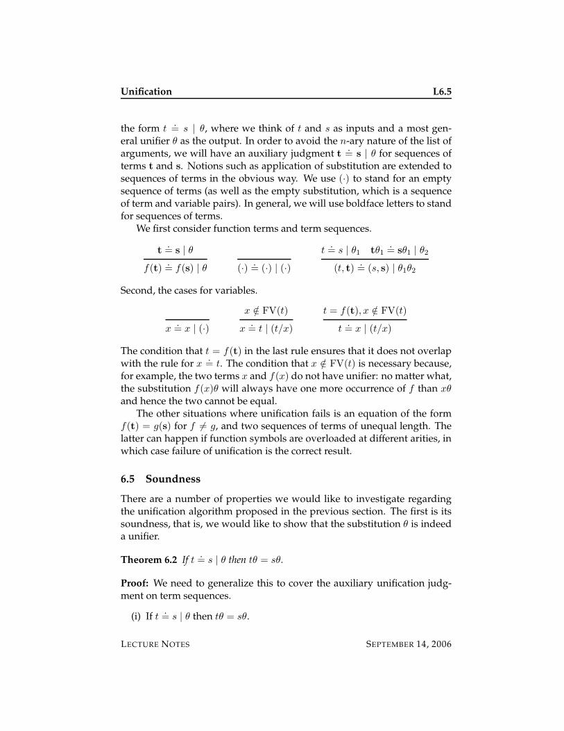
Unification L6.5
the form t.= s | θ, where we think of t and s as inputs and a most gen-
eral unifier θ as the output. In order to avoid the n-ary nature of the list ofarguments, we will have an auxiliary judgment t
.= s | θ for sequences of
terms t and s. Notions such as application of substitution are extended tosequences of terms in the obvious way. We use (·) to stand for an emptysequence of terms (as well as the empty substitution, which is a sequenceof term and variable pairs). In general, we will use boldface letters to standfor sequences of terms.
We first consider function terms and term sequences.
t.= s | θ
f(t).= f(s) | θ (·)
.= (·) | (·)
t.= s | θ1 tθ1
.= sθ1 | θ2
(t, t).= (s, s) | θ1θ2
Second, the cases for variables.
x.= x | (·)
x /∈ FV(t)
x.= t | (t/x)
t = f(t), x /∈ FV(t)
t.= x | (t/x)
The condition that t = f(t) in the last rule ensures that it does not overlapwith the rule for x
.= t. The condition that x /∈ FV(t) is necessary because,
for example, the two terms x and f(x) do not have unifier: no matter what,the substitution f(x)θ will always have one more occurrence of f than xθ
and hence the two cannot be equal.The other situations where unification fails is an equation of the form
f(t) = g(s) for f 6= g, and two sequences of terms of unequal length. Thelatter can happen if function symbols are overloaded at different arities, inwhich case failure of unification is the correct result.
6.5 Soundness
There are a number of properties we would like to investigate regardingthe unification algorithm proposed in the previous section. The first is itssoundness, that is, we would like to show that the substitution θ is indeeda unifier.
Theorem 6.2 If t.= s | θ then tθ = sθ.
Proof: We need to generalize this to cover the auxiliary unification judg-ment on term sequences.
(i) If t.= s | θ then tθ = sθ.
LECTURE NOTES SEPTEMBER 14, 2006
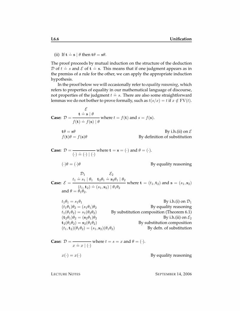
L6.6 Unification
(ii) If t.= s | θ then tθ = sθ.
The proof proceeds by mutual induction on the structure of the deductionD of t
.= s and E of t
.= s. This means that if one judgment appears as in
the premiss of a rule for the other, we can apply the appropriate inductionhypothesis.
In the proof below we will occasionally refer to equality reasoning, whichrefers to properties of equality in our mathematical language of discourse,not properties of the judgment t
.= s. There are also some straightforward
lemmas we do not bother to prove formally, such as t(s/x) = t if x /∈ FV(t).
Case: D =
Et
.= s | θ
f(t).= f(s) | θ
where t = f(t) and s = f(s).
tθ = sθ By i.h.(ii) on E
f(t)θ = f(s)θ By definition of substitution
Case: D =(·)
.= (·) | (·)
where t = s = (·) and θ = (·).
(·)θ = (·)θ By equality reasoning
Case: E =
D1
t1.= s1 | θ1
E2
t2θ1
.= s2θ1 | θ2
(t1, t2).= (s1, s2) | θ1θ2
where t = (t1, t2) and s = (s1, s2)
and θ = θ1θ2.
t1θ1 = s1θ1 By i.h.(i) on D1
(t1θ1)θ2 = (s1θ1)θ2 By equality reasoningt1(θ1θ2) = s1(θ2θ2) By substitution composition (Theorem 6.1)(t2θ1)θ2 = (s2θ1)θ2 By i.h.(ii) on E2
t2(θ1θ2) = s2(θ1θ2) By substitution composition(t1, t2)(θ1θ2) = (s1, s2)(θ1θ2) By defn. of substitution
Case: D =x
.= x | (·)
where t = s = x and θ = (·).
x(·) = x(·) By equality reasoning
LECTURE NOTES SEPTEMBER 14, 2006
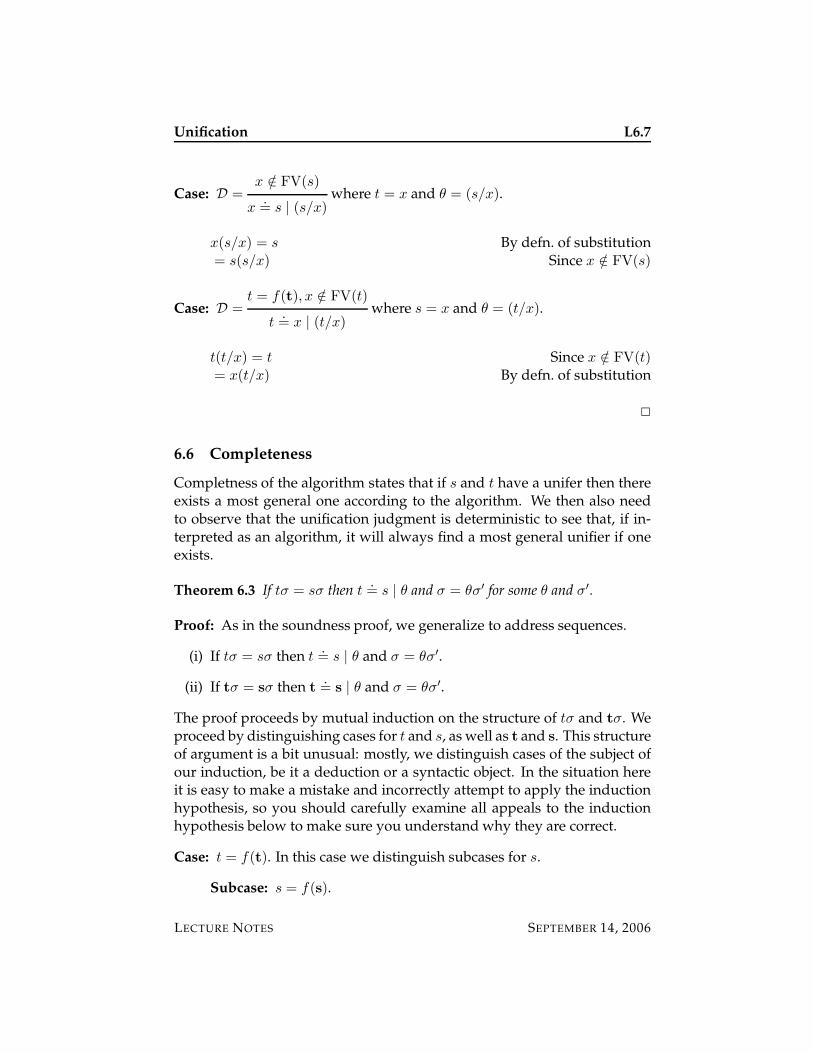
Unification L6.7
Case: D =x /∈ FV(s)
x.= s | (s/x)
where t = x and θ = (s/x).
x(s/x) = s By defn. of substitution= s(s/x) Since x /∈ FV(s)
Case: D =t = f(t), x /∈ FV(t)
t.= x | (t/x)
where s = x and θ = (t/x).
t(t/x) = t Since x /∈ FV(t)= x(t/x) By defn. of substitution
2
6.6 Completeness
Completness of the algorithm states that if s and t have a unifer then thereexists a most general one according to the algorithm. We then also needto observe that the unification judgment is deterministic to see that, if in-terpreted as an algorithm, it will always find a most general unifier if oneexists.
Theorem 6.3 If tσ = sσ then t.= s | θ and σ = θσ′ for some θ and σ′.
Proof: As in the soundness proof, we generalize to address sequences.
(i) If tσ = sσ then t.= s | θ and σ = θσ′.
(ii) If tσ = sσ then t.= s | θ and σ = θσ′.
The proof proceeds by mutual induction on the structure of tσ and tσ. Weproceed by distinguishing cases for t and s, as well as t and s. This structureof argument is a bit unusual: mostly, we distinguish cases of the subject ofour induction, be it a deduction or a syntactic object. In the situation hereit is easy to make a mistake and incorrectly attempt to apply the inductionhypothesis, so you should carefully examine all appeals to the inductionhypothesis below to make sure you understand why they are correct.
Case: t = f(t). In this case we distinguish subcases for s.
Subcase: s = f(s).
LECTURE NOTES SEPTEMBER 14, 2006
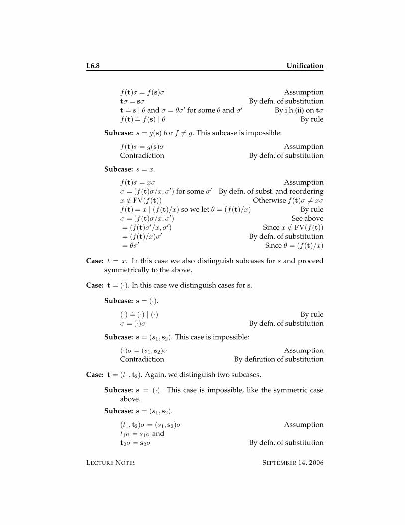
L6.8 Unification
f(t)σ = f(s)σ Assumptiontσ = sσ By defn. of substitutiont
.= s | θ and σ = θσ′ for some θ and σ′ By i.h.(ii) on tσ
f(t).= f(s) | θ By rule
Subcase: s = g(s) for f 6= g. This subcase is impossible:
f(t)σ = g(s)σ AssumptionContradiction By defn. of substitution
Subcase: s = x.
f(t)σ = xσ Assumptionσ = (f(t)σ/x, σ′) for some σ′ By defn. of subst. and reorderingx /∈ FV(f(t)) Otherwise f(t)σ 6= xσ
f(t) = x | (f(t)/x) so we let θ = (f(t)/x) By ruleσ = (f(t)σ/x, σ′) See above= (f(t)σ′/x, σ′) Since x /∈ FV(f(t))= (f(t)/x)σ′ By defn. of substitution= θσ′ Since θ = (f(t)/x)
Case: t = x. In this case we also distinguish subcases for s and proceedsymmetrically to the above.
Case: t = (·). In this case we distinguish cases for s.
Subcase: s = (·).
(·).= (·) | (·) By rule
σ = (·)σ By defn. of substitution
Subcase: s = (s1, s2). This case is impossible:
(·)σ = (s1, s2)σ AssumptionContradiction By definition of substitution
Case: t = (t1, t2). Again, we distinguish two subcases.
Subcase: s = (·). This case is impossible, like the symmetric caseabove.
Subcase: s = (s1, s2).
(t1, t2)σ = (s1, s2)σ Assumptiont1σ = s1σ andt2σ = s2σ By defn. of substitution
LECTURE NOTES SEPTEMBER 14, 2006
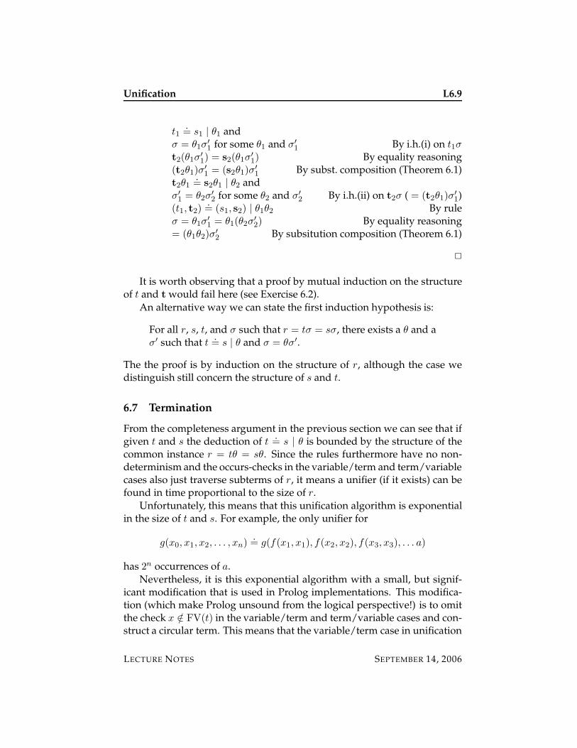
Unification L6.9
t1.= s1 | θ1 and
σ = θ1σ′
1for some θ1 and σ′
1By i.h.(i) on t1σ
t2(θ1σ′
1) = s2(θ1σ
′
1) By equality reasoning
(t2θ1)σ′
1= (s2θ1)σ
′
1By subst. composition (Theorem 6.1)
t2θ1
.= s2θ1 | θ2 and
σ′
1= θ2σ
′
2for some θ2 and σ′
2By i.h.(ii) on t2σ ( = (t2θ1)σ
′
1)
(t1, t2).= (s1, s2) | θ1θ2 By rule
σ = θ1σ′
1= θ1(θ2σ
′
2) By equality reasoning
= (θ1θ2)σ′
2By subsitution composition (Theorem 6.1)
2
It is worth observing that a proof by mutual induction on the structureof t and t would fail here (see Exercise 6.2).
An alternative way we can state the first induction hypothesis is:
For all r, s, t, and σ such that r = tσ = sσ, there exists a θ and aσ′ such that t
.= s | θ and σ = θσ′.
The the proof is by induction on the structure of r, although the case wedistinguish still concern the structure of s and t.
6.7 Termination
From the completeness argument in the previous section we can see that ifgiven t and s the deduction of t
.= s | θ is bounded by the structure of the
common instance r = tθ = sθ. Since the rules furthermore have no non-determinism and the occurs-checks in the variable/term and term/variablecases also just traverse subterms of r, it means a unifier (if it exists) can befound in time proportional to the size of r.
Unfortunately, this means that this unification algorithm is exponentialin the size of t and s. For example, the only unifier for
g(x0, x1, x2, . . . , xn).= g(f(x1, x1), f(x2, x2), f(x3, x3), . . . a)
has 2n occurrences of a.
Nevertheless, it is this exponential algorithm with a small, but signif-icant modification that is used in Prolog implementations. This modifica-tion (which make Prolog unsound from the logical perspective!) is to omitthe check x /∈ FV(t) in the variable/term and term/variable cases and con-struct a circular term. This means that the variable/term case in unification
LECTURE NOTES SEPTEMBER 14, 2006
L6.10 Unification
is constant time, because in an implementation we just change a pointer as-sociated with the variable to point to the term. This is of crucial importance,since unification in Prolog models parameter-passing from other languages(thinking of the predicate as a procedure), and it is not acceptable to taketime proportional to the size of the argument to invoke a procedure.
This observation notwithstanding, the worst-case complexity of the al-gorithm in Prolog is still exponential in the size of the input terms, but itis linear in the size of the result of unification. The latter fact appears to bewhat rescues this algorithm in practice, together with its straightforwardbehavior which is important for Prolog programmers.
All of this does not tell us what happens if we pass terms to our unifi-cation algorithm that do not have a unifier. It is not even obvious that thegiven rules terminate in that case (see Exercise 6.3). Fortunately, in practicemost non-unifiable terms result in a clash between function symbols ratherquickly.
6.8 Historical Notes
Unification was originally developed by Robinson [7] together with resolu-tion as a proof search principle. Both of these critically influenced the earlydesigns of Prolog, the first logic programming language. Similar computa-tions were described before, but not studied in their own right (see [1] formore on the history of unification).
It is possible to improve the complexity of unification to linear in thesize of the input terms if a different representation for the terms and sub-stitutions is chosen, such as a set of multi-equations [4, 5] or dag structureswith parent pointers [6]. These and similar algorithms are important insome applications [3], although in logic programming and general theoremproving, minor variants of Robinson’s original algorithm are prevalent.
Most modern versions of Prolog support sound unification, either asa separate predicate unify_with_occurs_check/2 or even as an optionalpart of the basic execution mechanism1. Given advanced compilation tech-nology, I have been quoted figures of 10% to 15% overhead for using soundunification, but I have not found a definitive study confirming this. We willreturn to the necessary optimization in a later lecture.
Another way out is to declare that the bug is a feature, and Prolog is re-ally a constraint programming language over rational trees, which requiresa small modification of the unification algorithm to ensure termination in
1for example, in Amzi!Prolog
LECTURE NOTES SEPTEMBER 14, 2006
Unification L6.11
the presence of circular terms [2] but still avoids the occurs-check. The priceto be paid is that the connection to the predicate calculus is lost, and thatpopular reasoning techniques such as induction are much more difficult toapply in the presence of infinite terms.
6.9 Exercises
Exercise 6.1 Prove τ(σθ) = (τσ)θ under the conditions stated in Theorem 6.1.
Exercise 6.2 Show precisely where and why the attempt to prove completeness ofthe rules for unification by mutual induction over the structure of t and t (insteadof tσ and tσ) would fail.
Exercise 6.3 Show that the rules for unification terminate no matter whethergiven unifiable or non-unifiable terms t and s. Together with soundness, com-pleteness, and determinacy of the rules this means that they constitute a decisionprocedure for finding a most general unifier if it exists.
6.10 References
[1] Franz Baader and Wayne Snyder. Unification theory. In J.A. Robinsonand A. Voronkov, editors, Handbook of Automated Reasoning, volume 1,chapter 8, pages 447–532. Elsevier and MIT Press, 2001.
[2] Joxan Jaffar. Efficient unification over infinite terms. New GenerationComputing, 2(3):207–219, 1984.
[3] Kevin Knight. Unification: A multi-disciplinary survey. ACM Comput-ing Surveys, 2(1):93–124, March 1989.
[4] Alberto Martelli and Ugo Montanari. Unification in linear time andspace: A structured presentation. Internal Report B76-16, Istituto diElaborazione delle Informazione, Consiglio Nazionale delle Ricerche,Pisa, Italy, July 1976.
[5] Alberto Martelli and Ugo Montanari. An efficient unification al-gorithm. ACM Transactions on Programming Languages and Systems,4(2):258–282, April 1982.
[6] M. S. Paterson and M. N. Wegman. Linear unification. Journal of Com-puter and System Sciences, 16(2):158–167, April 1978.
[7] J. A. Robinson. A machine-oriented logic based on the resolution prin-ciple. Journal of the ACM, 12(1):23–41, January 1965.
LECTURE NOTES SEPTEMBER 14, 2006

L6.12 Unification
LECTURE NOTES SEPTEMBER 14, 2006
15-819K: Logic Programming
Lecture 7
Lifting
Frank Pfenning
September 19, 2006
Lifting is the name for turning a search calculus with ground judgmentsinto one employing free variables. Unification might be viewed as theresult of lifting a ground equality judgment, but we never explicitly in-troduced such a judgment. In this lecture our goal is to lift previouslygiven operational semantics judgments for logic programming to permitfree variables and prove their soundness and completeness. Unificationand the judgment to compute most general unifiers are the central tools.
7.1 Explicating Rule Application
When explicating the left-to-right subgoal selection order in the operationalsemantics, we needed to introduce conjunction and truth in order to exposethese choices explicitly. When explicating the first-to-last strategy of clauseselection and backtracking we need to introduce disjunction and falsehood.It should therefore come as no surprise that in order to explicit the details ofrule application and unification we need some further logical connectives.These include at least universal quantification and implication. However,we will for the moment postpone their formal treatment in order to con-centrate on the integration of unification from the previous lecture into theoperational semantics.
An inference ruleB true
P true
is modeled logically as the proposition
∀x1 . . . ∀xn. B ⊃ P
LECTURE NOTES SEPTEMBER 19, 2006
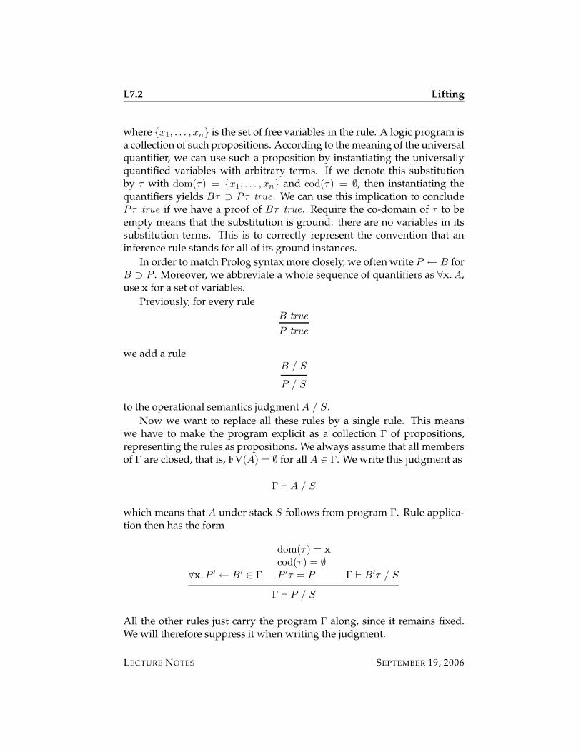
L7.2 Lifting
where {x1, . . . , xn} is the set of free variables in the rule. A logic program isa collection of such propositions. According to the meaning of the universalquantifier, we can use such a proposition by instantiating the universallyquantified variables with arbitrary terms. If we denote this substitutionby τ with dom(τ) = {x1, . . . , xn} and cod(τ) = ∅, then instantiating thequantifiers yields Bτ ⊃ Pτ true . We can use this implication to concludePτ true if we have a proof of Bτ true . Require the co-domain of τ to beempty means that the substitution is ground: there are no variables in itssubstitution terms. This is to correctly represent the convention that aninference rule stands for all of its ground instances.
In order to match Prolog syntax more closely, we often write P ← B forB ⊃ P . Moreover, we abbreviate a whole sequence of quantifiers as ∀x. A,use x for a set of variables.
Previously, for every rule
B true
P true
we add a ruleB / S
P / S
to the operational semantics judgment A / S.
Now we want to replace all these rules by a single rule. This meanswe have to make the program explicit as a collection Γ of propositions,representing the rules as propositions. We always assume that all membersof Γ are closed, that is, FV(A) = ∅ for all A ∈ Γ. We write this judgment as
Γ ` A / S
which means that A under stack S follows from program Γ. Rule applica-tion then has the form
∀x. P ′ ← B′ ∈ Γ
dom(τ) = x
cod(τ) = ∅P ′τ = P Γ ` B′τ / S
Γ ` P / S
All the other rules just carry the program Γ along, since it remains fixed.We will therefore suppress it when writing the judgment.
LECTURE NOTES SEPTEMBER 19, 2006
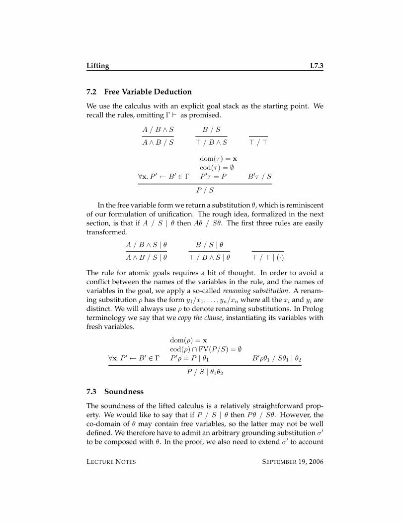
Lifting L7.3
7.2 Free Variable Deduction
We use the calculus with an explicit goal stack as the starting point. Werecall the rules, omitting Γ ` as promised.
A / B ∧ S
A ∧B / S
B / S
> / B ∧ S > / >
∀x. P ′ ← B′ ∈ Γ
dom(τ) = x
cod(τ) = ∅P ′τ = P B′τ / S
P / S
In the free variable form we return a substitution θ, which is reminiscentof our formulation of unification. The rough idea, formalized in the nextsection, is that if A / S | θ then Aθ / Sθ. The first three rules are easilytransformed.
A / B ∧ S | θ
A ∧B / S | θ
B / S | θ
> / B ∧ S | θ > / > | (·)
The rule for atomic goals requires a bit of thought. In order to avoid aconflict between the names of the variables in the rule, and the names ofvariables in the goal, we apply a so-called renaming substitution. A renam-ing substitution ρ has the form y1/x1, . . . , yn/xn where all the xi and yi aredistinct. We will always use ρ to denote renaming substitutions. In Prologterminology we say that we copy the clause, instantiating its variables withfresh variables.
∀x. P ′ ← B′ ∈ Γ
dom(ρ) = x
cod(ρ) ∩ FV(P/S) = ∅P ′ρ
.= P | θ1 B′ρθ1 / Sθ1 | θ2
P / S | θ1θ2
7.3 Soundness
The soundness of the lifted calculus is a relatively straightforward prop-erty. We would like to say that if P / S | θ then Pθ / Sθ. However, theco-domain of θ may contain free variables, so the latter may not be welldefined. We therefore have to admit an arbitrary grounding substitution σ′
to be composed with θ. In the proof, we also need to extend σ′ to account
LECTURE NOTES SEPTEMBER 19, 2006
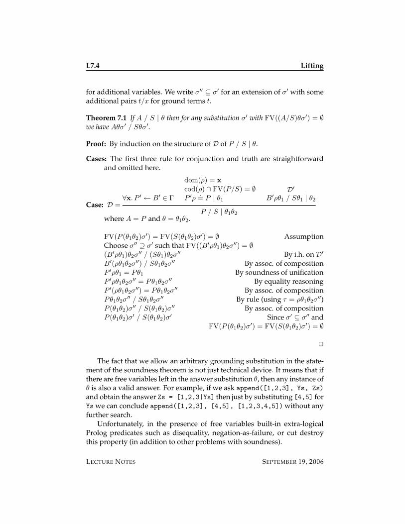
L7.4 Lifting
for additional variables. We write σ′′ ⊆ σ′ for an extension of σ′ with someadditional pairs t/x for ground terms t.
Theorem 7.1 If A / S | θ then for any substitution σ′ with FV((A/S)θσ′) = ∅we have Aθσ′ / Sθσ′.
Proof: By induction on the structure of D of P / S | θ.
Cases: The first three rule for conjunction and truth are straightforwardand omitted here.
Case: D =∀x. P ′ ← B′ ∈ Γ
dom(ρ) = x
cod(ρ) ∩ FV(P/S) = ∅P ′ρ
.= P | θ1
D′
B′ρθ1 / Sθ1 | θ2
P / S | θ1θ2
where A = P and θ = θ1θ2.
FV(P (θ1θ2)σ′) = FV(S(θ1θ2)σ
′) = ∅ AssumptionChoose σ′′ ⊇ σ′ such that FV((B′ρθ1)θ2σ
′′) = ∅(B′ρθ1)θ2σ
′′ / (Sθ1)θ2σ′′ By i.h. on D′
B′(ρθ1θ2σ′′) / Sθ1θ2σ
′′ By assoc. of compositionP ′ρθ1 = Pθ1 By soundness of unificationP ′ρθ1θ2σ
′′ = Pθ1θ2σ′′ By equality reasoning
P ′(ρθ1θ2σ′′) = Pθ1θ2σ
′′ By assoc. of compositionPθ1θ2σ
′′ / Sθ1θ2σ′′ By rule (using τ = ρθ1θ2σ
′′)P (θ1θ2)σ
′′ / S(θ1θ2)σ′′ By assoc. of composition
P (θ1θ2)σ′ / S(θ1θ2)σ
′ Since σ′ ⊆ σ′′ andFV(P (θ1θ2)σ
′) = FV(S(θ1θ2)σ′) = ∅
2
The fact that we allow an arbitrary grounding substitution in the state-ment of the soundness theorem is not just technical device. It means that ifthere are free variables left in the answer substitution θ, then any instance ofθ is also a valid answer. For example, if we ask append([1,2,3], Ys, Zs)
and obtain the answer Zs = [1,2,3|Ys] then just by substituting [4,5] forYs we can conclude append([1,2,3], [4,5], [1,2,3,4,5]) without anyfurther search.
Unfortunately, in the presence of free variables built-in extra-logicalProlog predicates such as disequality, negation-as-failure, or cut destroythis property (in addition to other problems with soundness).
LECTURE NOTES SEPTEMBER 19, 2006
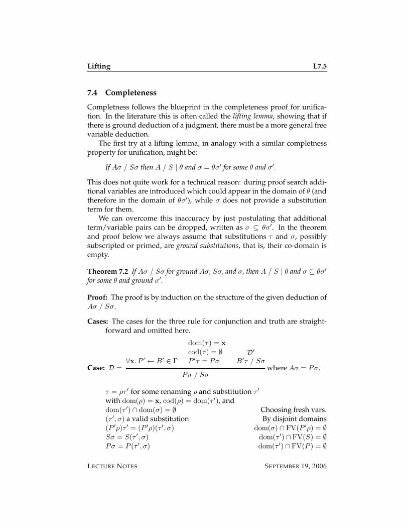
Lifting L7.5
7.4 Completeness
Completness follows the blueprint in the completeness proof for unifica-tion. In the literature this is often called the lifting lemma, showing that ifthere is ground deduction of a judgment, there must be a more general freevariable deduction.
The first try at a lifting lemma, in analogy with a similar completnessproperty for unification, might be:
If Aσ / Sσ then A / S | θ and σ = θσ′ for some θ and σ′.
This does not quite work for a technical reason: during proof search addi-tional variables are introduced which could appear in the domain of θ (andtherefore in the domain of θσ′), while σ does not provide a substitutionterm for them.
We can overcome this inaccuracy by just postulating that additionalterm/variable pairs can be dropped, written as σ ⊆ θσ′. In the theoremand proof below we always assume that substitutions τ and σ, possiblysubscripted or primed, are ground substitutions, that is, their co-domain isempty.
Theorem 7.2 If Aσ / Sσ for ground Aσ, Sσ, and σ, then A / S | θ and σ ⊆ θσ′
for some θ and ground σ′.
Proof: The proof is by induction on the structure of the given deduction ofAσ / Sσ.
Cases: The cases for the three rule for conjunction and truth are straight-forward and omitted here.
Case: D =∀x. P ′ ← B′ ∈ Γ
dom(τ) = x
cod(τ) = ∅P ′τ = Pσ
D′
B′τ / Sσ
Pσ / Sσwhere Aσ = Pσ.
τ = ρτ ′ for some renaming ρ and substitution τ ′
with dom(ρ) = x, cod(ρ) = dom(τ ′), anddom(τ ′) ∩ dom(σ) = ∅ Choosing fresh vars.(τ ′, σ) a valid substitution By disjoint domains(P ′ρ)τ ′ = (P ′ρ)(τ ′, σ) dom(σ) ∩ FV(P ′ρ) = ∅Sσ = S(τ ′, σ) dom(τ ′) ∩ FV(S) = ∅Pσ = P (τ ′, σ) dom(τ ′) ∩ FV(P ) = ∅
LECTURE NOTES SEPTEMBER 19, 2006
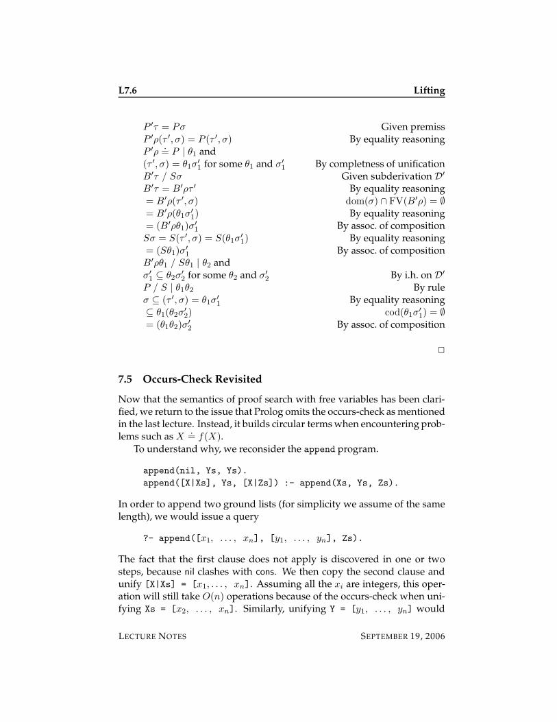
L7.6 Lifting
P ′τ = Pσ Given premissP ′ρ(τ ′, σ) = P (τ ′, σ) By equality reasoningP ′ρ
.= P | θ1 and
(τ ′, σ) = θ1σ′
1for some θ1 and σ′
1By completness of unification
B′τ / Sσ Given subderivation D′
B′τ = B′ρτ ′ By equality reasoning= B′ρ(τ ′, σ) dom(σ) ∩ FV(B′ρ) = ∅= B′ρ(θ1σ
′
1) By equality reasoning
= (B′ρθ1)σ′
1By assoc. of composition
Sσ = S(τ ′, σ) = S(θ1σ′
1) By equality reasoning
= (Sθ1)σ′
1By assoc. of composition
B′ρθ1 / Sθ1 | θ2 andσ′
1⊆ θ2σ
′
2for some θ2 and σ′
2By i.h. on D′
P / S | θ1θ2 By ruleσ ⊆ (τ ′, σ) = θ1σ
′
1By equality reasoning
⊆ θ1(θ2σ′
2) cod(θ1σ
′
1) = ∅
= (θ1θ2)σ′
2By assoc. of composition
2
7.5 Occurs-Check Revisited
Now that the semantics of proof search with free variables has been clari-fied, we return to the issue that Prolog omits the occurs-check as mentionedin the last lecture. Instead, it builds circular terms when encountering prob-lems such as X
.= f(X).
To understand why, we reconsider the append program.
append(nil, Ys, Ys).
append([X|Xs], Ys, [X|Zs]) :- append(Xs, Ys, Zs).
In order to append two ground lists (for simplicity we assume of the samelength), we would issue a query
?- append([x1, . . . , xn], [y1, . . . , yn], Zs).
The fact that the first clause does not apply is discovered in one or twosteps, because nil clashes with cons. We then copy the second clause andunify [X|Xs] = [x1, . . . , xn]. Assuming all the xi are integers, this oper-ation will still take O(n) operations because of the occurs-check when uni-fying Xs = [x2, . . . , xn]. Similarly, unifying Y = [y1, . . . , yn] would
LECTURE NOTES SEPTEMBER 19, 2006
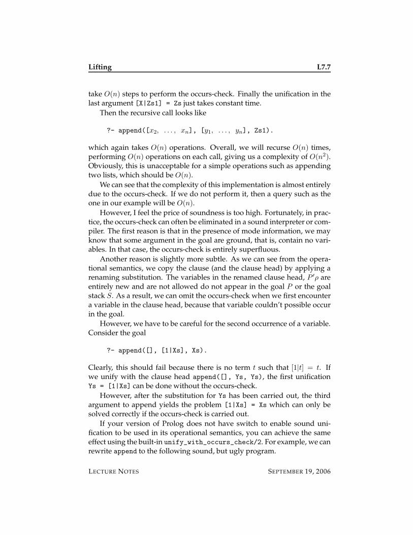
Lifting L7.7
take O(n) steps to perform the occurs-check. Finally the unification in thelast argument [X|Zs1] = Zs just takes constant time.
Then the recursive call looks like
?- append([x2, . . . , xn], [y1, . . . , yn], Zs1).
which again takes O(n) operations. Overall, we will recurse O(n) times,performing O(n) operations on each call, giving us a complexity of O(n2).Obviously, this is unacceptable for a simple operations such as appendingtwo lists, which should be O(n).
We can see that the complexity of this implementation is almost entirelydue to the occurs-check. If we do not perform it, then a query such as theone in our example will be O(n).
However, I feel the price of soundness is too high. Fortunately, in prac-tice, the occurs-check can often be eliminated in a sound interpreter or com-piler. The first reason is that in the presence of mode information, we mayknow that some argument in the goal are ground, that is, contain no vari-ables. In that case, the occurs-check is entirely superfluous.
Another reason is slightly more subtle. As we can see from the opera-tional semantics, we copy the clause (and the clause head) by applying arenaming substitution. The variables in the renamed clause head, P ′ρ areentirely new and are not allowed do not appear in the goal P or the goalstack S. As a result, we can omit the occurs-check when we first encountera variable in the clause head, because that variable couldn’t possible occurin the goal.
However, we have to be careful for the second occurrence of a variable.Consider the goal
?- append([], [1|Xs], Xs).
Clearly, this should fail because there is no term t such that [1|t] = t. Ifwe unify with the clause head append([], Ys, Ys), the first unificationYs = [1|Xs] can be done without the occurs-check.
However, after the substitution for Ys has been carried out, the thirdargument to append yields the problem [1|Xs] = Xs which can only besolved correctly if the occurs-check is carried out.
If your version of Prolog does not have switch to enable sound uni-fication to be used in its operational semantics, you can achieve the sameeffect using the built-in unify_with_occurs_check/2. For example, we canrewrite append to the following sound, but ugly program.
LECTURE NOTES SEPTEMBER 19, 2006
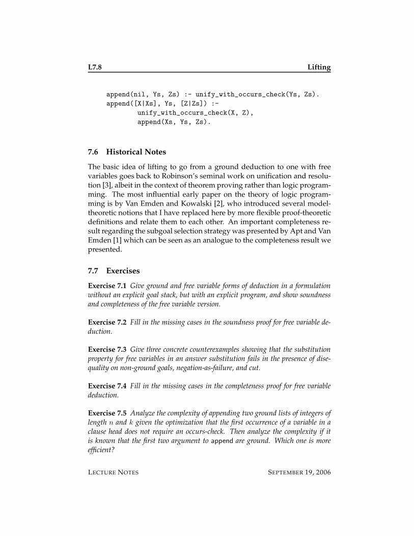
L7.8 Lifting
append(nil, Ys, Zs) :- unify_with_occurs_check(Ys, Zs).
append([X|Xs], Ys, [Z|Zs]) :-
unify_with_occurs_check(X, Z),
append(Xs, Ys, Zs).
7.6 Historical Notes
The basic idea of lifting to go from a ground deduction to one with freevariables goes back to Robinson’s seminal work on unification and resolu-tion [3], albeit in the context of theorem proving rather than logic program-ming. The most influential early paper on the theory of logic program-ming is by Van Emden and Kowalski [2], who introduced several model-theoretic notions that I have replaced here by more flexible proof-theoreticdefinitions and relate them to each other. An important completeness re-sult regarding the subgoal selection strategy was presented by Apt and VanEmden [1] which can be seen as an analogue to the completeness result wepresented.
7.7 Exercises
Exercise 7.1 Give ground and free variable forms of deduction in a formulationwithout an explicit goal stack, but with an explicit program, and show soundnessand completeness of the free variable version.
Exercise 7.2 Fill in the missing cases in the soundness proof for free variable de-duction.
Exercise 7.3 Give three concrete counterexamples showing that the substitutionproperty for free variables in an answer substitution fails in the presence of dise-quality on non-ground goals, negation-as-failure, and cut.
Exercise 7.4 Fill in the missing cases in the completeness proof for free variablededuction.
Exercise 7.5 Analyze the complexity of appending two ground lists of integers oflength n and k given the optimization that the first occurrence of a variable in aclause head does not require an occurs-check. Then analyze the complexity if itis known that the first two argument to append are ground. Which one is moreefficient?
LECTURE NOTES SEPTEMBER 19, 2006
Lifting L7.9
7.8 References
[1] Krzysztof R. Apt and M. H. Van Emden. Contributions to the theory oflogic programming. Journal of the ACM, 29(3):841–862, July 1982.
[2] M. H. Van Emden and R. A. Kowalski. The semantics of predicate logicas a programming language. Journal of the ACM, 23(4):733–742, October1976.
[3] J. A. Robinson. A machine-oriented logic based on the resolution prin-ciple. Journal of the ACM, 12(1):23–41, January 1965.
LECTURE NOTES SEPTEMBER 19, 2006

L7.10 Lifting
LECTURE NOTES SEPTEMBER 19, 2006
15-819K: Logic Programming
Lecture 8
Completion
Frank Pfenning
September 21, 2006
In this lecture we extend the ground backtracking semantics to permit freevariables. This requires a stronger normal form for programs. After intro-ducing this normal form related to the so-call iff-completion of a program,we give the semantics at which point we have a complete specification ofthe pure Prolog search behavior including unification, subgoal selectionand backtracking. At this point we return to the logical meaning of Prologprograms and derive the iff-completion of a program via a process calledresiduation.
8.1 Existential Quantification
First we return to the backtracking semantics with the intent of adding freevariables and unification to make it a fully specified semantics for pureProlog.
The first problem is presented by the rules for atomic goals. In a groundcalculus, the rule
∀x. P ′ ← B′ ∈ Γ
dom(τ) = x
cod(τ) = ∅P ′τ = P B′τ / S / F
P / S / F
is correct only if we stipulate that for every ground atomic goal P there isexactly one program clause for which the rule above can be applied. Other-wise, not all failure or choice points would be explicit in the semantics.
LECTURE NOTES SEPTEMBER 21, 2006
L8.2 Completion
Now we need the property that for every atomic goal P (potentiallycontaining free variables) there is exactly one program clause that applies.Because goals can have the form p(X1, . . . ,Xn) for variables X1, . . . ,Xn,this means that for every predicate p there should be only one clause inthe program. Moreover, the head of this clause must unify with every per-missible goal. At first this may seem far-fetched, but since our extendedlanguage includes equality, we can actually achieve this by transformingthe program so that all clause heads have the form p(X1, . . . ,Xn) for dis-tinct variables X1, . . . ,Xn.
As an example, consider the member predicate in the form appropriatefor the ground semantics.
member(X, []) :- fail.
member(X, [Y|Ys]) :- X = Y ; member(X, Ys).
We can transform this further by factoring the two cases as
member(X, Ys) :-
(Ys = [], fail) ;
(Ys = [Y|Ys1], (X = Y ; member(X, Ys1))).
This can be simplified, because the first disjunct will always fail.
member(X, Ys) :- Ys = [Y|Ys1], (X = Y ; member(X, Ys1)).
Writing such a program would be considered poor style, since the very firstone is much easier to read. However, as an internal representation it turnsout to be convenient.
We take one more step which, unfortunately, does not have a simplerendering in all implementations of Prolog. We can simplify the treatmentof atomic goals further if the only free variables in a clause are the onesappearing in the head. In the member example above, this is not the case,because Y and Ys1 occur in the body, but not the head. If we had existen-tial quantification ∃x.A, we could overcome this. In logical form, the rulewould be the following.
∃y.∃ys1. Y s.= [y|ys1] ∧ (X
.= y ∨member(X, ys1)) true
member(X,Y s) true
In some implementations of Prolog, existential quantification is availablewith the syntax X^A for ∃x.A.1 Then the program above would read
1You should beware, however, that some implementations of this are unsound in thatthe variable X is visible outside its scope.
LECTURE NOTES SEPTEMBER 21, 2006
Completion L8.3
member(X, Ys) :-
Y^Ys1^(Ys = [Y|Ys1], (X = Y ; member(X, Ys1))).
On the logical side, This requires a new form of proposition, ∃x.A,where x is a bound variable with scope A. We assume that we can alwaysrename bound variables. For example, we consider ∃x.∃y. p(x, x, y) and∃y.∃z. p(y, y, z) to be identical. We also assume that bound variables (writ-ten as lower-case identifiers) and free variables (written as upper-case iden-tifiers) are distinct syntactic classes, so no clash between them can arise.
Strictly speaking we should differentiate between substitutions for vari-ables x that may be bound, and for logic variables X (also called meta-variables). At this point, the necessary machinery for this distinction wouldyield little benefit, so we use the same notations and postulate the sameproperties for both.
Existential quantification is now defined by
A(t/x) true
∃x.A true∃I
where the the substitution term t is understood to have no free variablessince logical deduction is ground deduction.
When carrying out a substitution θ, we must take care when encounter-ing a quantifier ∃x.A. If x is in the domain of θ, we should first rename it toavoid possible confusion between the bound x and the x that θ substitutesfor. The second condition is that x does not occur in the co-domain of θ.This condition is actually vacuous here (t is closed), but required in moregeneral settings.
(∃x.A)θ = ∃x. (Aθ) provided x /∈ dom(θ) ∪ cod(θ)
Recall the convention that bound variables can always be silently renamed,so we can always satisfy the side condition no matter what θ is.
The search semantics for existential quantification comes in two flavors:in the ground version we guess the correct term t, in the free variable ver-sion we substitute a fresh logic variable.
A(t/x) / S
∃x.A / S
A(X/x) / S | θ X /∈ FV(∃x.A / S)
∃x.A / S | θ
Since X does not occur in ∃x.A / S, we could safely restrict θ in the con-clusion to remove any substitution term for X.
LECTURE NOTES SEPTEMBER 21, 2006
L8.4 Completion
8.2 Backtracking Semantics with Free Variables
Now we assume the program is in a normal form where for each atomicpredicate p of arity n there is exactly one clause
∀x1 . . . ∀xn. p(x1, . . . xn)← B′
where the FV(B′) ⊆ {x1, . . . , xn}.
We will not endeavor to return the answer substitution from the freevariable judgment, but just describe the computation to either success orfailure. The extension to compute an answer substitution requires somethought, but does not add any essentially new elements (see Exercise 8.1).Therefore, the we write A / S / F where A, S, and F may have freevariables. The intended interpretation is that if A / S / F in the freevariable semantics then there exists a grounding substitution σ such thatAσ / Sσ / Fσ in the ground semantics. This is not very precise, but suffi-cient for our purposes.
First, the rules for conjunction and truth. They are the same in the freeand ground semantics.
A / B ∧ S / F
A ∧B / S / F
B / S / F
> / B ∧ S / F > / > / F
Second, the rules for disjunction and falsehood. Again, it plays no role ifthe goals are interpreted as closed or with free variables.
A / S / (B ∧ S) ∨ F
A ∨B / S / F
B / S′ / F
⊥ / S / (B ∧ S′) ∨ F
fails (no rule)
⊥ / S / ⊥
Third, the equality rules. Clearly, these involve unification, so substitutionscome into play.
t.= s | θ > / Sθ / F
t.= s / S / F
there is no θ with t.= s | θ ⊥ / S / F
t.= s / S / F
When unification succeeds, the most general unifier θ must be applied tothe success continuation S which shares variables with t and s. But wedo not apply the substitution to F . Consider a goal of the form (X
.= a ∧
p(X)) ∨ (X.= b∧ q(X)) to see that while we try the first disjunction, X
.= a
the instantiations of X should not affect the failure continuation.
LECTURE NOTES SEPTEMBER 21, 2006
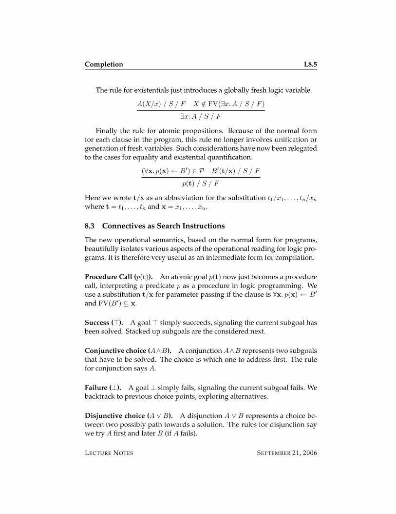
Completion L8.5
The rule for existentials just introduces a globally fresh logic variable.
A(X/x) / S / F X /∈ FV(∃x.A / S / F )
∃x.A / S / F
Finally the rule for atomic propositions. Because of the normal formfor each clause in the program, this rule no longer involves unification orgeneration of fresh variables. Such considerations have now been relegatedto the cases for equality and existential quantification.
(∀x. p(x)← B′) ∈ P B′(t/x) / S / F
p(t) / S / F
Here we wrote t/x as an abbreviation for the substitution t1/x1, . . . , tn/xn
where t = t1, . . . , tn and x = x1, . . . , xn.
8.3 Connectives as Search Instructions
The new operational semantics, based on the normal form for programs,beautifully isolates various aspects of the operational reading for logic pro-grams. It is therefore very useful as an intermediate form for compilation.
Procedure Call (p(t)). An atomic goal p(t) now just becomes a procedurecall, interpreting a predicate p as a procedure in logic programming. Weuse a substitution t/x for parameter passing if the clause is ∀x. p(x) ← B′
and FV(B′) ⊆ x.
Success (>). A goal > simply succeeds, signaling the current subgoal hasbeen solved. Stacked up subgoals are the considered next.
Conjunctive choice (A∧B). A conjunction A∧B represents two subgoalsthat have to be solved. The choice is which one to address first. The rulefor conjunction says A.
Failure (⊥). A goal ⊥ simply fails, signaling the current subgoal fails. Webacktrack to previous choice points, exploring alternatives.
Disjunctive choice (A ∨ B). A disjunction A ∨ B represents a choice be-tween two possibly path towards a solution. The rules for disjunction saywe try A first and later B (if A fails).
LECTURE NOTES SEPTEMBER 21, 2006
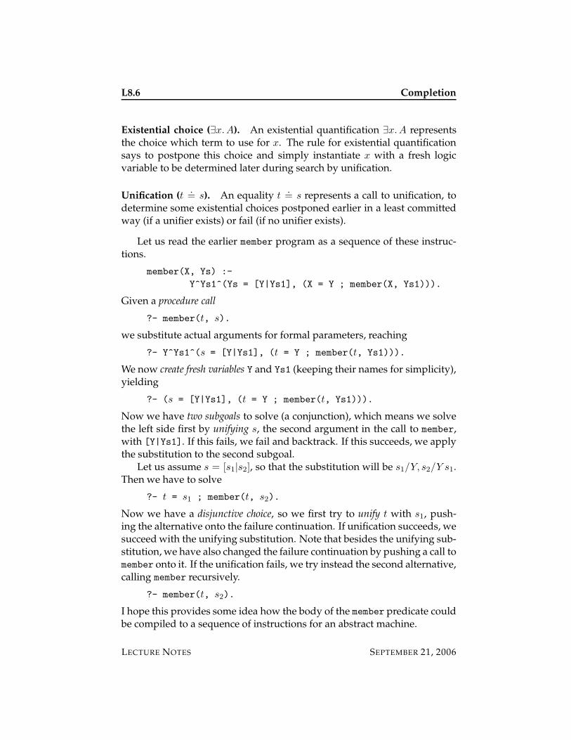
L8.6 Completion
Existential choice (∃x.A). An existential quantification ∃x.A representsthe choice which term to use for x. The rule for existential quantificationsays to postpone this choice and simply instantiate x with a fresh logicvariable to be determined later during search by unification.
Unification (t.= s). An equality t
.= s represents a call to unification, to
determine some existential choices postponed earlier in a least committedway (if a unifier exists) or fail (if no unifier exists).
Let us read the earlier member program as a sequence of these instruc-tions.
member(X, Ys) :-
Y^Ys1^(Ys = [Y|Ys1], (X = Y ; member(X, Ys1))).
Given a procedure call
?- member(t, s).
we substitute actual arguments for formal parameters, reaching
?- Y^Ys1^(s = [Y|Ys1], (t = Y ; member(t, Ys1))).
We now create fresh variables Y and Ys1 (keeping their names for simplicity),yielding
?- (s = [Y|Ys1], (t = Y ; member(t, Ys1))).
Now we have two subgoals to solve (a conjunction), which means we solvethe left side first by unifying s, the second argument in the call to member,with [Y|Ys1]. If this fails, we fail and backtrack. If this succeeds, we applythe substitution to the second subgoal.
Let us assume s = [s1|s2], so that the substitution will be s1/Y, s2/Y s1.Then we have to solve
?- t = s1 ; member(t, s2).
Now we have a disjunctive choice, so we first try to unify t with s1, push-ing the alternative onto the failure continuation. If unification succeeds, wesucceed with the unifying substitution. Note that besides the unifying sub-stitution, we have also changed the failure continuation by pushing a call tomember onto it. If the unification fails, we try instead the second alternative,calling member recursively.
?- member(t, s2).
I hope this provides some idea how the body of the member predicate couldbe compiled to a sequence of instructions for an abstract machine.
LECTURE NOTES SEPTEMBER 21, 2006
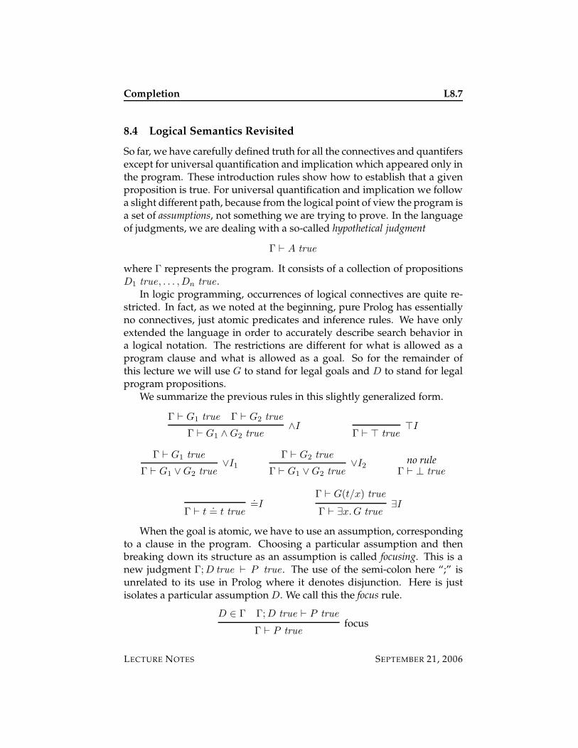
Completion L8.7
8.4 Logical Semantics Revisited
So far, we have carefully defined truth for all the connectives and quantifersexcept for universal quantification and implication which appeared only inthe program. These introduction rules show how to establish that a givenproposition is true. For universal quantification and implication we followa slight different path, because from the logical point of view the program isa set of assumptions, not something we are trying to prove. In the languageof judgments, we are dealing with a so-called hypothetical judgment
Γ ` A true
where Γ represents the program. It consists of a collection of propositionsD1 true, . . . ,Dn true .
In logic programming, occurrences of logical connectives are quite re-stricted. In fact, as we noted at the beginning, pure Prolog has essentiallyno connectives, just atomic predicates and inference rules. We have onlyextended the language in order to accurately describe search behavior ina logical notation. The restrictions are different for what is allowed as aprogram clause and what is allowed as a goal. So for the remainder ofthis lecture we will use G to stand for legal goals and D to stand for legalprogram propositions.
We summarize the previous rules in this slightly generalized form.
Γ ` G1 true Γ ` G2 true
Γ ` G1 ∧G2 true∧I
Γ ` > true>I
Γ ` G1 true
Γ ` G1 ∨G2 true∨I1
Γ ` G2 true
Γ ` G1 ∨G2 true∨I2
no ruleΓ ` ⊥ true
Γ ` t.= t true
.=I
Γ ` G(t/x) true
Γ ` ∃x.G true∃I
When the goal is atomic, we have to use an assumption, correspondingto a clause in the program. Choosing a particular assumption and thenbreaking down its structure as an assumption is called focusing. This is anew judgment Γ;D true ` P true . The use of the semi-colon here “;” isunrelated to its use in Prolog where it denotes disjunction. Here is justisolates a particular assumption D. We call this the focus rule.
D ∈ Γ Γ;D true ` P true
Γ ` P truefocus
LECTURE NOTES SEPTEMBER 21, 2006
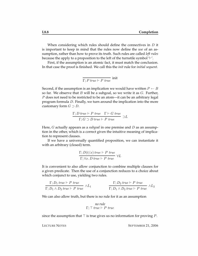
L8.8 Completion
When considering which rules should define the connectives in D itis important to keep in mind that the rules now define the use of an as-sumption, rather than how to prove its truth. Such rules are called left rulesbecause the apply to a proposition to the left of the turnstile symbol ‘`’.
First, if the assumption is an atomic fact, it must match the conclusion.In that case the proof is finished. We call this the init rule for initial sequent.
Γ;P true ` P trueinit
Second, if the assumption is an implication we would have written P ← B
so far. We observe that B will be a subgoal, so we write it as G. Further,P does not need to be restricted to be an atom—it can be an arbitrary legalprogram formula D. Finally, we turn around the implication into the morecustomary form G ⊃ D.
Γ;D true ` P true Γ ` G true
Γ;G ⊃ D true ` P true⊃L
Here, G actually appears as a subgoal in one premise and D as an assump-tion in the other, which is a correct given the intuitive meaning of implica-tion to represent clauses.
If we have a universally quantified proposition, we can instantiate itwith an arbitrary (closed) term.
Γ;D(t/x) true ` P true
Γ;∀x.D true ` P true∀L
It is convenient to also allow conjunction to combine multiple clauses fora given predicate. Then the use of a conjunction reduces to a choice aboutwhich conjunct to use, yielding two rules.
Γ;D1 true ` P true
Γ;D1 ∧D2 true ` P true∧L1
Γ;D2 true ` P true
Γ;D1 ∧D2 true ` P true∧L2
We can also allow truth, but there is no rule for it as an assumption
no ruleΓ;> true ` P true
since the assumption that > is true gives us no information for proving P .
LECTURE NOTES SEPTEMBER 21, 2006
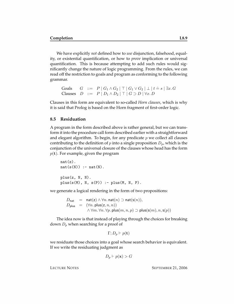
Completion L8.9
We have explicitly not defined how to use disjunction, falsehood, equal-ity, or existential quantification, or how to prove implication or universalquantification. This is because attempting to add such rules would sig-nificantly change the nature of logic programming. From the rules, we canread off the restriction to goals and program as conforming to the followinggrammar.
Goals G ::= P | G1 ∧G2 | > | G1 ∨G2 | ⊥ | t.= s | ∃x.G
Clauses D ::= P | D1 ∧D2 | > | G ⊃ D | ∀x.D
Clauses in this form are equivalent to so-called Horn clauses, which is whyit is said that Prolog is based on the Horn fragment of first-order logic.
8.5 Residuation
A program in the form described above is rather general, but we can trans-form it into the procedure call form described earlier with a straightforwardand elegant algorithm. To begin, for any predicate p we collect all clausescontributing to the definition of p into a single proposition Dp, which is theconjunction of the universal closure of the clauses whose head has the formp(t). For example, given the program
nat(z).
nat(s(N)) :- nat(N).
plus(z, N, N).
plus(s(M), N, s(P)) :- plus(M, N, P).
we generate a logical rendering in the form of two propositions:
Dnat = nat(z) ∧ ∀n. nat(n) ⊃ nat(s(n)),Dplus = (∀n. plus(z, n, n))
∧ ∀m.∀n.∀p. plus(m,n, p) ⊃ plus(s(m), n, s(p))
The idea now is that instead of playing through the choices for breakingdown Dp when searching for a proof of
Γ;Dp ` p(t)
we residuate those choices into a goal whose search behavior is equivalent.If we write the residuating judgment as
Dp ` p(x) > G
LECTURE NOTES SEPTEMBER 21, 2006
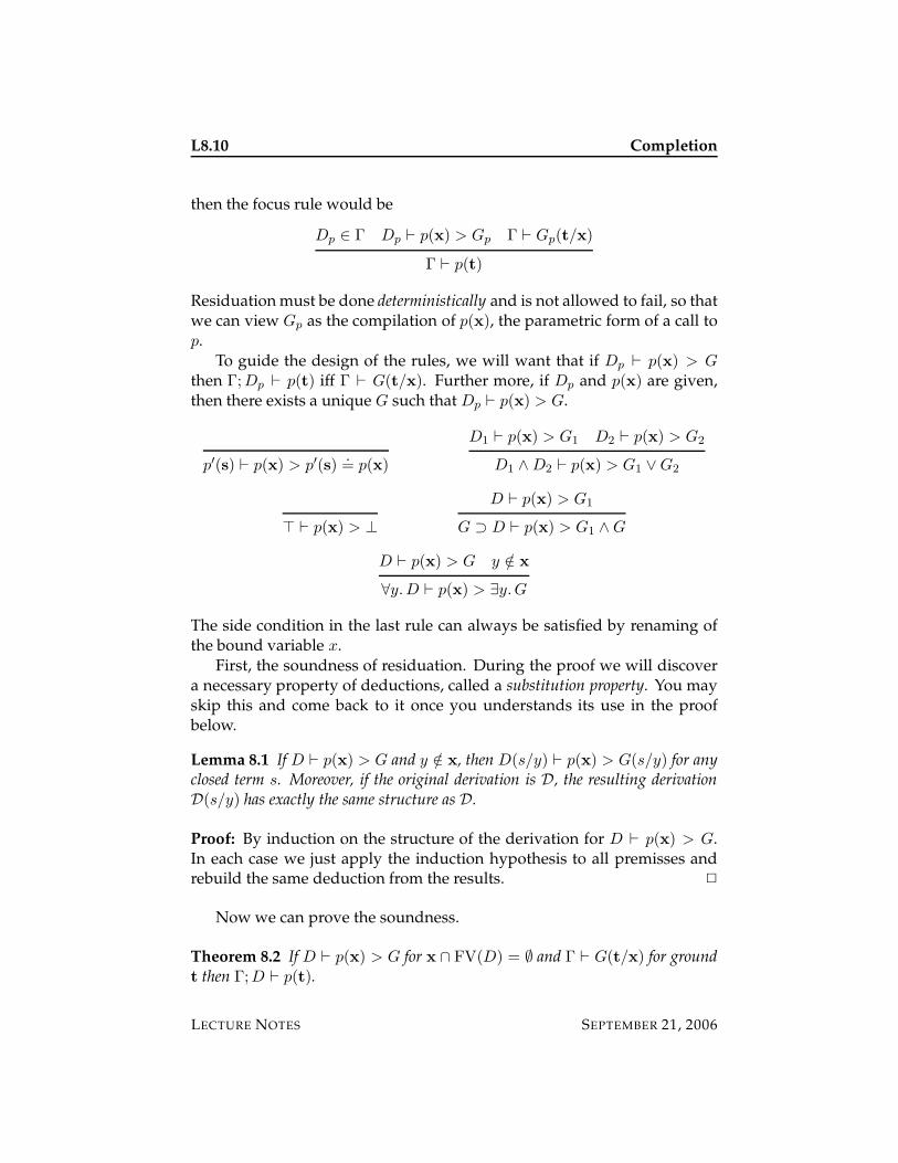
L8.10 Completion
then the focus rule would be
Dp ∈ Γ Dp ` p(x) > Gp Γ ` Gp(t/x)
Γ ` p(t)
Residuation must be done deterministically and is not allowed to fail, so thatwe can view Gp as the compilation of p(x), the parametric form of a call top.
To guide the design of the rules, we will want that if Dp ` p(x) > G
then Γ;Dp ` p(t) iff Γ ` G(t/x). Further more, if Dp and p(x) are given,then there exists a unique G such that Dp ` p(x) > G.
p′(s) ` p(x) > p′(s).= p(x)
D1 ` p(x) > G1 D2 ` p(x) > G2
D1 ∧D2 ` p(x) > G1 ∨G2
> ` p(x) > ⊥
D ` p(x) > G1
G ⊃ D ` p(x) > G1 ∧G
D ` p(x) > G y /∈ x
∀y.D ` p(x) > ∃y.G
The side condition in the last rule can always be satisfied by renaming ofthe bound variable x.
First, the soundness of residuation. During the proof we will discovera necessary property of deductions, called a substitution property. You mayskip this and come back to it once you understands its use in the proofbelow.
Lemma 8.1 If D ` p(x) > G and y /∈ x, then D(s/y) ` p(x) > G(s/y) for anyclosed term s. Moreover, if the original derivation is D, the resulting derivationD(s/y) has exactly the same structure as D.
Proof: By induction on the structure of the derivation for D ` p(x) > G.In each case we just apply the induction hypothesis to all premisses andrebuild the same deduction from the results. 2
Now we can prove the soundness.
Theorem 8.2 If D ` p(x) > G for x ∩ FV(D) = ∅ and Γ ` G(t/x) for groundt then Γ;D ` p(t).
LECTURE NOTES SEPTEMBER 21, 2006
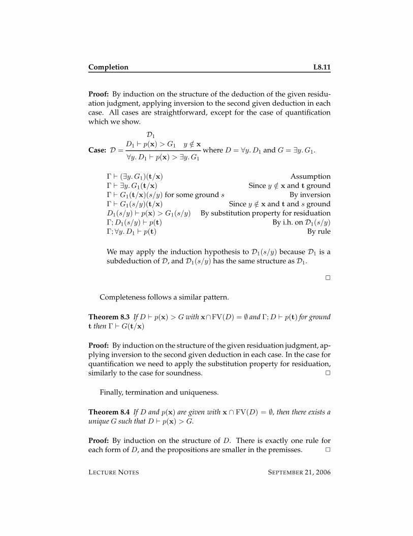
Completion L8.11
Proof: By induction on the structure of the deduction of the given residu-ation judgment, applying inversion to the second given deduction in eachcase. All cases are straightforward, except for the case of quantificationwhich we show.
Case: D =
D1
D1 ` p(x) > G1 y /∈ x
∀y.D1 ` p(x) > ∃y.G1
where D = ∀y.D1 and G = ∃y.G1.
Γ ` (∃y.G1)(t/x) AssumptionΓ ` ∃y.G1(t/x) Since y /∈ x and t groundΓ ` G1(t/x)(s/y) for some ground s By inversionΓ ` G1(s/y)(t/x) Since y /∈ x and t and s groundD1(s/y) ` p(x) > G1(s/y) By substitution property for residuationΓ;D1(s/y) ` p(t) By i.h. on D1(s/y)Γ;∀y.D1 ` p(t) By rule
We may apply the induction hypothesis to D1(s/y) because D1 is asubdeduction of D, and D1(s/y) has the same structure as D1.
2
Completeness follows a similar pattern.
Theorem 8.3 If D ` p(x) > G with x∩FV(D) = ∅ and Γ;D ` p(t) for groundt then Γ ` G(t/x)
Proof: By induction on the structure of the given residuation judgment, ap-plying inversion to the second given deduction in each case. In the case forquantification we need to apply the substitution property for residuation,similarly to the case for soundness. 2
Finally, termination and uniqueness.
Theorem 8.4 If D and p(x) are given with x ∩ FV(D) = ∅, then there exists aunique G such that D ` p(x) > G.
Proof: By induction on the structure of D. There is exactly one rule foreach form of D, and the propositions are smaller in the premisses. 2
LECTURE NOTES SEPTEMBER 21, 2006
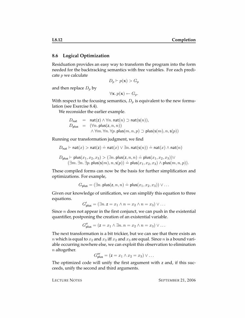
L8.12 Completion
8.6 Logical Optimization
Residuation provides an easy way to transform the program into the formneeded for the backtracking semantics with free variables. For each predi-cate p we calculate
Dp ` p(x) > Gp
and then replace Dp by∀x. p(x)← Gp.
With respect to the focusing semantics, Dp is equivalent to the new formu-lation (see Exercise 8.4).
We reconsider the earlier example.
Dnat = nat(z) ∧ ∀n. nat(n) ⊃ nat(s(n)),Dplus = (∀n. plus(z, n, n))
∧ ∀m.∀n.∀p. plus(m,n, p) ⊃ plus(s(m), n, s(p))
Running our transformation judgment, we find
Dnat ` nat(x) > nat(z).= nat(x) ∨ ∃n. nat(s(n))
.= nat(x) ∧ nat(n)
Dplus ` plus(x1, x2, x3) > (∃n. plus(z, n, n).= plus(x1, x2, x3))∨
(∃m.∃n.∃p. plus(s(m), n, s(p)).= plus(x1, x2, x3) ∧ plus(m,n, p)).
These compiled forms can now be the basis for further simplification andoptimizations. For example,
Gplus = (∃n. plus(z, n, n).= plus(x1, x2, x3)) ∨ . . .
Given our knowledge of unification, we can simplify this equation to threeequations.
G′
plus = (∃n. z = x1 ∧ n = x2 ∧ n = x3) ∨ . . .
Since n does not appear in the first conjunct, we can push in the existentialquantifier, postponing the creation of an existential variable.
G′′
plus = (z = x1 ∧ ∃n. n = x2 ∧ n = x3) ∨ . . .
The next transformation is a bit trickier, but we can see that there exists ann which is equal to x2 and x3 iff x2 and x3 are equal. Since n is a bound vari-able occurring nowhere else, we can exploit this observation to eliminationn altogether.
G′′′
plus = (z = x1 ∧ x2 = x3) ∨ . . .
The optimized code will unify the first argument with z and, if this suc-ceeds, unify the second and third arguments.
LECTURE NOTES SEPTEMBER 21, 2006
Completion L8.13
8.7 Iff Completion
We now revisit the normal form ∀x. p(x) ← Gp. Since this represents theonly way of succeeding in a proof of p(t), we can actually turn the implica-tion around, replacing it by an if and only if (↔)
∀x. p(x)↔ Gp.
Of course, this proposition is outside the fragment that is amenable to logicprogramming search (considering the right-to-left implication), but it hasfound some application in the notion of definitional reflection, where it isusually written as
∀x. p(x)4
= Gp.
This allows us to draw conclusions that the program alone does not permit,specifically about the falsehood of propositions.
We do not have the formal reasoning rules available to us at this point,but given the (slightly optimized) iff-completion of nat,
∀x. nat(x)↔ z.= x ∨ ∃n. s(n)
.= x ∧ nat(n)
we would be able to prove, explicitly with formal rules, that nat(a) is falsefor a new constant a, because a is neither equal to z nor to s(n) for some n.
Unfortunately the expressive power of the completion is still quite lim-ited in that it is much weaker than induction.
8.8 Historical Notes
The notion of iff-completion goes back to Clark [2] who investigated no-tions of negation and their justification in the early years of logic program-ming.
The use of goal-directed search and focusing to explain logic program-ming goes back to Miller et al. [3], who tested various extensions of thelogic presented here for suitability as the foundation for a logic program-ming language.
The use of residuation for compilation and optimization has been pro-posed by Cervesato [1], who also shows that the ideas are quite robust byaddressing a much richer logic.
The notion of definitional reflection goes back to Schroeder-Heister [5]who also examined its relationship to completion [4]. More recently, reflec-tion has been employed in a theorem prover derived from logic program-ming [6] in the Bedwyr system.
LECTURE NOTES SEPTEMBER 21, 2006
L8.14 Completion
8.9 Exercises
Exercise 8.1 Extend the free variable semantics with backtracking to explicitlyreturn an answer substitution θ. State the soundness and completness of thissemantics with respect to the one that does not explicitly calculate the answer sub-stitution. If you feel brave, prove these two theorems.
Exercise 8.2 Prove that the free variable backtracking semantics given in lectureis sound and complete with respect to the ground semantics.
Exercise 8.3 Prove the completeness of residuation.
Exercise 8.4 Given soundness and completeness of residuation, show that if wereplace programs Dp by ∀x. p(x)← Gp where Dp ` p(x) > Gp then the focusingsemantics is preserved.
8.10 References
[1] Iliano Cervesato. Proof-theoretic foundation of compilation in logicprogramming languages. In J. Jaffar, editor, Proceedings of the Joint In-ternational Conference and Symposium on Logic Programming (JICSLP’98),pages 115–129, Manchester, England, June 1998. MIT Press.
[2] Keith L. Clark. Negation as failure. In H. Gallaire and J. Minker, edi-tors, Logic and Databases, pages 293–322. Plenum Press, New York, 1978.
[3] Dale Miller, Gopalan Nadathur, Frank Pfenning, and Andre Scedrov.Uniform proofs as a foundation for logic programming. Annals of Pureand Applied Logic, 51:125–157, 1991.
[4] Peter Schroeder-Heister. Definitional reflection and the completion.In R. Dyckhoff, editor, Proceedings of the 4th International Workshop onExtensions of Logic Programming, pages 333–347. Springer-Verlag LNCS798, March 1993.
[5] Peter Schroeder-Heister. Rules of definitional reflection. In M. Vardi,editor, Proceedings of the 8th Annual Symposium on Logic in computer Sci-ence (LICS’93), pages 222–232, Montreal, Canada, July 1993. IEEE Com-puter Society Press.
[6] Alwen Tiu, Gopalan Nadathur, and Dale Miller. Mixing finite suc-cess and finite failure in an automated prover. In C.Benzmuller,J.Harrison, and C.Schurmann, editors, Proceedings of the Workshop onEmpirically Successful Automated Reasnoing in Higher-Order Logics (ES-HOL’05), pages 79–98, Montego Bay, Jamaica, December 2005.
LECTURE NOTES SEPTEMBER 21, 2006
15-819K: Logic Programming
Lecture 9
Types
Frank Pfenning
September 26, 2006
In this lecture we introduce types into logic programming, primarily todistinguish meaningful from meaningless terms and propositions, therebycapturing errors early during program development.
9.1 Views on Types
Types are a multi-faceted concept, and also subject of much debate. Wewill discuss some of the views that have been advanced regarding the roleof types in logic programming, and then focus on the one we find mostuseful and interesting.
Descriptive Types. In logic programming terminology, a type system iscalled descriptive if it captures some aspect of program behavior, where pro-gram behavior is defined entirely without reference to types. A commonexample is to think of a type as an approximation to the success set of theprogram, that is, the set of terms on which it holds. Reconsider addition onunary numbers:
plus(z, N, N).
plus(s(M), N, s(P)) :- plus(M, N, P).
We can see that if plus(t1, t2, t3) is true according to this definition, thent1 must be a natural number, that is, nat(t1) according to the definition
nat(z).
nat(s(N)) :- nat(N).
LECTURE NOTES SEPTEMBER 26, 2006
L9.2 Types
On the other hand, nothing interesting can be said about the other twoarguments, because the first clause as written permits non-sensical propo-sitions such as plus(z, [], []) to be true.
The nature of descriptive types means that usually they are used to opti-mize program behavior rather than as an aid to the programmer for writingcorrect code.
Prescriptive Types. A type system is called prescriptive if it is an integralpart of the meaning of programs. In the example above, if we prescribethat plus is a relation between three terms of type nat, then we suddenlydifferentiate well-typed expressions (such as plus(z, s(z), P) when P isa variable of type nat) from expressions that are not well-typed and there-fore meaningless (such as plus(z, [], []). Among the well-typed ex-pressions we then further distinguish those propositions which are trueand those which are false.
Prescriptive types, in a well-designed type system, are immediatelyuseful to the programmer since many accidental mistakes in the programwill be captured rather then leading to either failure or success, which maybe very difficult to debug. In some ways, the situation in pure Prolog isworse than in other dynamically typed languages such as Lisp, because inthe latter language you will often get a run-time error for incorrect pro-grams, while in pure Prolog everything is either true or false. This is some-what overstates the case, since many built-in predicates have dynamicallyenforced type restrictions. Nevertheless programming with no static andfew dynamic errors becomes more and more difficult as programs growlarger. I recognize that it may be somewhat difficult to fully appreciate thepoint if you write only small programs as you do in this class (at least sofar).
Within the prescriptive type approach, we can make further distinctionas to the way types are checked or expressed.
Monadic Propositions as Types. In this approach types are representedas monadic predicates, such as nat above. This approach is prevalent inthe early logic programming literature, and it is also the prevalent viewclassical logic. The standard answer to the question why the traditionalpredicate calculus (also known as classical first-order logic) is untyped isthat types can be eliminated in favor of monadic predicates. For example,we can translate ∀x:nat. A into ∀x. nat(x) ⊃ A, where x now ranges overarbitrary terms. Similarly, ∃x:nat. A becomes ∃x. nat(x) ∧A.
LECTURE NOTES SEPTEMBER 26, 2006
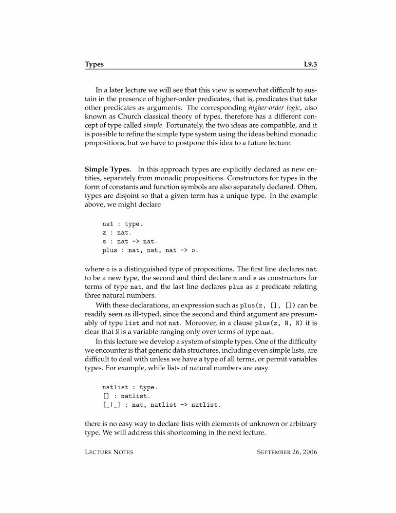
Types L9.3
In a later lecture we will see that this view is somewhat difficult to sus-tain in the presence of higher-order predicates, that is, predicates that takeother predicates as arguments. The corresponding higher-order logic, alsoknown as Church classical theory of types, therefore has a different con-cept of type called simple. Fortunately, the two ideas are compatible, and itis possible to refine the simple type system using the ideas behind monadicpropositions, but we have to postpone this idea to a future lecture.
Simple Types. In this approach types are explicitly declared as new en-tities, separately from monadic propositions. Constructors for types in theform of constants and function symbols are also separately declared. Often,types are disjoint so that a given term has a unique type. In the exampleabove, we might declare
nat : type.
z : nat.
s : nat -> nat.
plus : nat, nat, nat -> o.
where o is a distinguished type of propositions. The first line declares natto be a new type, the second and third declare z and s as constructors forterms of type nat, and the last line declares plus as a predicate relatingthree natural numbers.
With these declarations, an expression such as plus(z, [], []) can bereadily seen as ill-typed, since the second and third argument are presum-ably of type list and not nat. Moreover, in a clause plus(z, N, N) it isclear that N is a variable ranging only over terms of type nat.
In this lecture we develop a system of simple types. One of the difficultywe encounter is that generic data structures, including even simple lists, aredifficult to deal with unless we have a type of all terms, or permit variablestypes. For example, while lists of natural numbers are easy
natlist : type.
[] : natlist.
[_|_] : nat, natlist -> natlist.
there is no easy way to declare lists with elements of unknown or arbitrarytype. We will address this shortcoming in the next lecture.
LECTURE NOTES SEPTEMBER 26, 2006
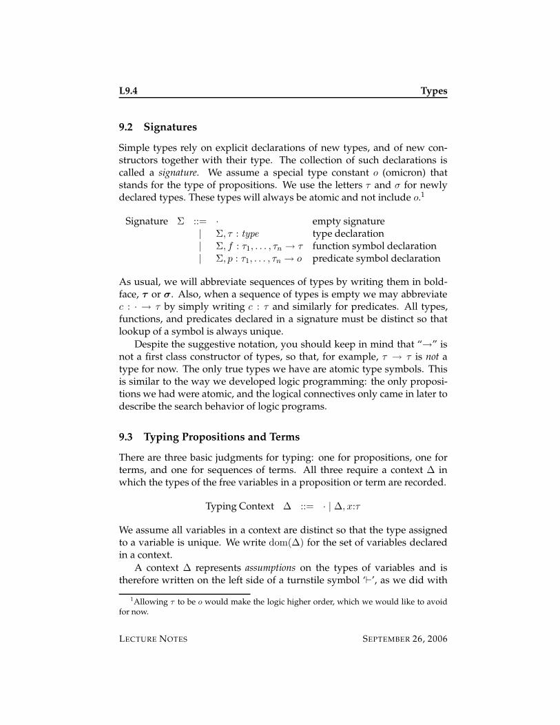
L9.4 Types
9.2 Signatures
Simple types rely on explicit declarations of new types, and of new con-structors together with their type. The collection of such declarations iscalled a signature. We assume a special type constant o (omicron) thatstands for the type of propositions. We use the letters τ and σ for newlydeclared types. These types will always be atomic and not include o.1
Signature Σ ::= · empty signature| Σ, τ : type type declaration| Σ, f : τ1, . . . , τn → τ function symbol declaration| Σ, p : τ1, . . . , τn → o predicate symbol declaration
As usual, we will abbreviate sequences of types by writing them in bold-face, τ or σ. Also, when a sequence of types is empty we may abbreviatec : · → τ by simply writing c : τ and similarly for predicates. All types,functions, and predicates declared in a signature must be distinct so thatlookup of a symbol is always unique.
Despite the suggestive notation, you should keep in mind that “→” isnot a first class constructor of types, so that, for example, τ → τ is not atype for now. The only true types we have are atomic type symbols. Thisis similar to the way we developed logic programming: the only proposi-tions we had were atomic, and the logical connectives only came in later todescribe the search behavior of logic programs.
9.3 Typing Propositions and Terms
There are three basic judgments for typing: one for propositions, one forterms, and one for sequences of terms. All three require a context ∆ inwhich the types of the free variables in a proposition or term are recorded.
Typing Context ∆ ::= · | ∆, x:τ
We assume all variables in a context are distinct so that the type assignedto a variable is unique. We write dom(∆) for the set of variables declaredin a context.
A context ∆ represents assumptions on the types of variables and istherefore written on the left side of a turnstile symbol ‘`’, as we did with
1Allowing τ to be o would make the logic higher order, which we would like to avoidfor now.
LECTURE NOTES SEPTEMBER 26, 2006
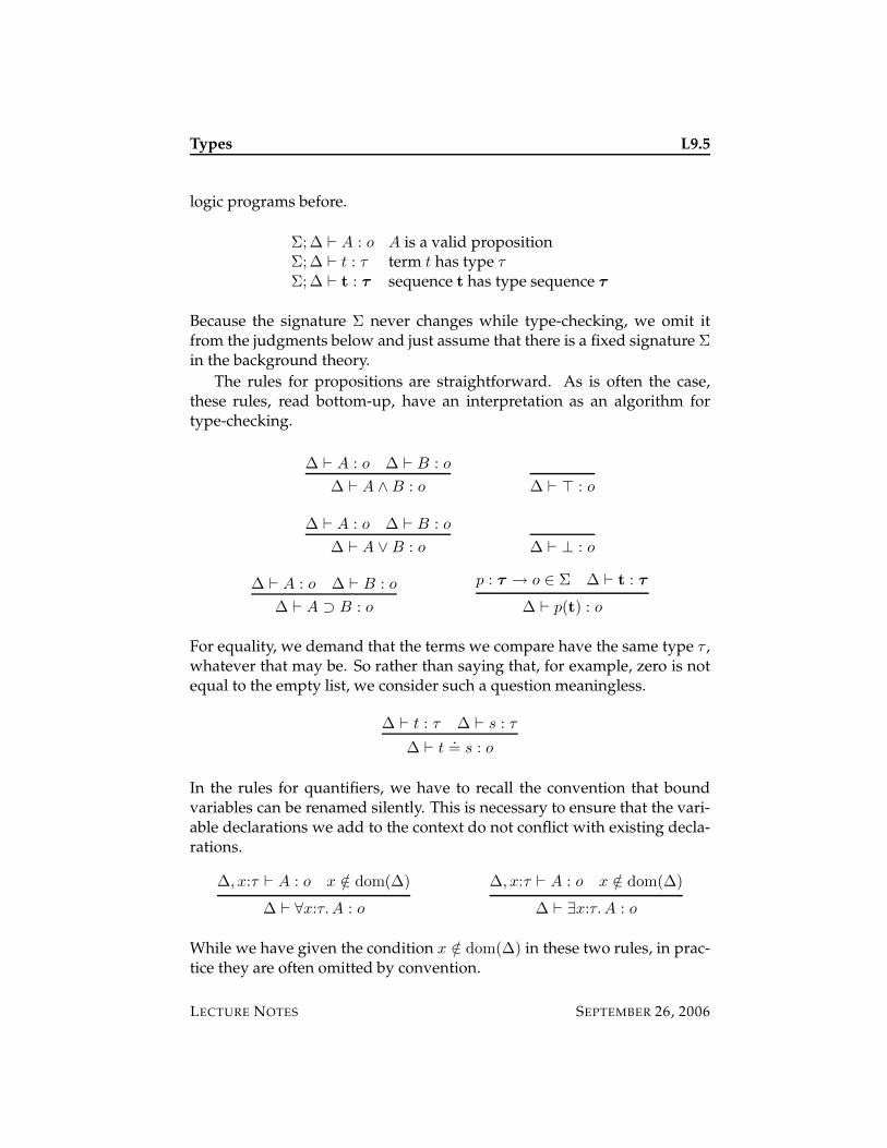
Types L9.5
logic programs before.
Σ;∆ ` A : o A is a valid propositionΣ;∆ ` t : τ term t has type τ
Σ;∆ ` t : τ sequence t has type sequence τ
Because the signature Σ never changes while type-checking, we omit itfrom the judgments below and just assume that there is a fixed signature Σin the background theory.
The rules for propositions are straightforward. As is often the case,these rules, read bottom-up, have an interpretation as an algorithm fortype-checking.
∆ ` A : o ∆ ` B : o
∆ ` A ∧B : o ∆ ` > : o
∆ ` A : o ∆ ` B : o
∆ ` A ∨B : o ∆ ` ⊥ : o
∆ ` A : o ∆ ` B : o
∆ ` A ⊃ B : o
p : τ → o ∈ Σ ∆ ` t : τ
∆ ` p(t) : o
For equality, we demand that the terms we compare have the same type τ ,whatever that may be. So rather than saying that, for example, zero is notequal to the empty list, we consider such a question meaningless.
∆ ` t : τ ∆ ` s : τ
∆ ` t.= s : o
In the rules for quantifiers, we have to recall the convention that boundvariables can be renamed silently. This is necessary to ensure that the vari-able declarations we add to the context do not conflict with existing decla-rations.
∆, x:τ ` A : o x /∈ dom(∆)
∆ ` ∀x:τ.A : o
∆, x:τ ` A : o x /∈ dom(∆)
∆ ` ∃x:τ.A : o
While we have given the condition x /∈ dom(∆) in these two rules, in prac-tice they are often omitted by convention.
LECTURE NOTES SEPTEMBER 26, 2006
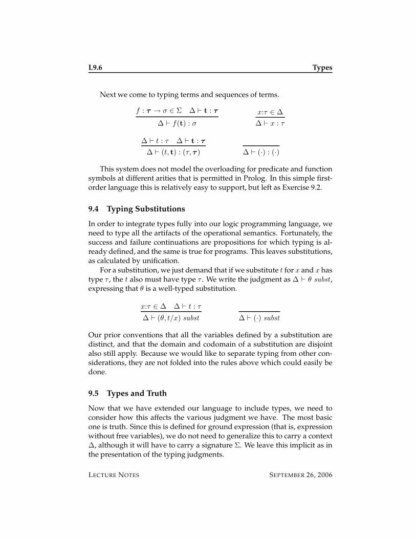
L9.6 Types
Next we come to typing terms and sequences of terms.
f : τ → σ ∈ Σ ∆ ` t : τ
∆ ` f(t) : σ
x:τ ∈ ∆
∆ ` x : τ
∆ ` t : τ ∆ ` t : τ
∆ ` (t, t) : (τ, τ ) ∆ ` (·) : (·)
This system does not model the overloading for predicate and functionsymbols at different arities that is permitted in Prolog. In this simple first-order language this is relatively easy to support, but left as Exercise 9.2.
9.4 Typing Substitutions
In order to integrate types fully into our logic programming language, weneed to type all the artifacts of the operational semantics. Fortunately, thesuccess and failure continuations are propositions for which typing is al-ready defined, and the same is true for programs. This leaves substitutions,as calculated by unification.
For a substitution, we just demand that if we substitute t for x and x hastype τ , the t also must have type τ . We write the judgment as ∆ ` θ subst ,expressing that θ is a well-typed substitution.
x:τ ∈ ∆ ∆ ` t : τ
∆ ` (θ, t/x) subst ∆ ` (·) subst
Our prior conventions that all the variables defined by a substitution aredistinct, and that the domain and codomain of a substitution are disjointalso still apply. Because we would like to separate typing from other con-siderations, they are not folded into the rules above which could easily bedone.
9.5 Types and Truth
Now that we have extended our language to include types, we need toconsider how this affects the various judgment we have. The most basicone is truth. Since this is defined for ground expression (that is, expressionwithout free variables), we do not need to generalize this to carry a context∆, although it will have to carry a signature Σ. We leave this implicit as inthe presentation of the typing judgments.
LECTURE NOTES SEPTEMBER 26, 2006

Types L9.7
We presuppose that any proposition we write is a well-typed proposi-tion, that is, has type o. In other words, if we write A true we implicitlyassume that · ` A : o. We have to be careful that our rules maintain thisproperty, and in which direction the rule is read. For example, when therule
Γ ` A true
Γ ` A ∨B true∨I
is read from the premiss to the conclusion, then we would need a secondpremiss to check that B : o.
However, we prefer to read it as “Assuming A ∨ B is a valid proposition,A ∨B is true if A is true.” In this reading, the condition on B is implicit.
Since the bottom-up reading of rules is pervasive in logic programming,we will adopt the same here. Then, only the rules for quantifiers require anadditional typing premiss. Recall that Γ represents a fixed program.
· ` t : τ Γ ` A(t/x) true
Γ ` ∃x:τ.A true∃I
· ` t : τ Γ;A(t/x) true ` P true
Γ;∀x:τ.A ` P true∀L
This assumes that if we substitute a term of type τ for a variable of type τ ,the result will remain well-typed. Fortunately, this property holds and iseasy to prove.
Theorem 9.1 Assume ∆ ` θ subst .
1. If ∆ ` t : τ then ∆ ` tθ : τ .
2. If ∆ ` t : τ then ∆ ` tθ : τ .
3. If ∆ ` A : o then ∆ ` Aθ : o.
Proof: By mututal induction on the structure of the given typing deriva-tions for t, t, and A. 2
9.6 Type Preservation
A critical property tying together a type system with the operational se-mantics for a programming language is type preservation. It expresses thatif we start in a well-typed state, during the execution of a program all in-termediate states will be well-typed. This is an absolutely fundamentalproperty without which a type system does not make much sense. Eitherthe type system or the operational semantics needs to be revised in such acase so that they match at least to this extent.
LECTURE NOTES SEPTEMBER 26, 2006
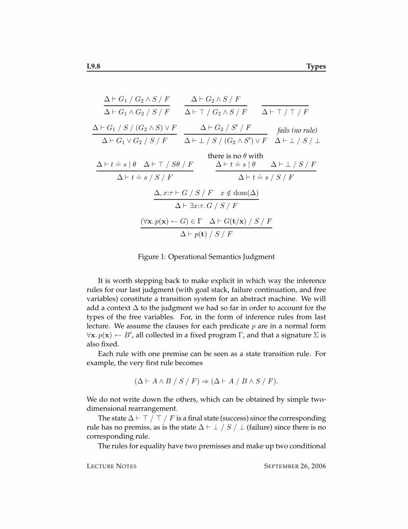
L9.8 Types
∆ ` G1 / G2 ∧ S / F
∆ ` G1 ∧G2 / S / F
∆ ` G2 ∧ S / F
∆ ` > / G2 ∧ S / F ∆ ` > / > / F
∆ ` G1 / S / (G2 ∧ S) ∨ F
∆ ` G1 ∨G2 / S / F
∆ ` G2 / S′ / F
∆ ` ⊥ / S / (G2 ∧ S′) ∨ F
fails (no rule)
∆ ` ⊥ / S / ⊥
∆ ` t.= s | θ ∆ ` > / Sθ / F
∆ ` t.= s / S / F
there is no θ with∆ ` t
.= s | θ ∆ ` ⊥ / S / F
∆ ` t.= s / S / F
∆, x:τ ` G / S / F x /∈ dom(∆)
∆ ` ∃x:τ.G / S / F
(∀x. p(x)← G) ∈ Γ ∆ ` G(t/x) / S / F
∆ ` p(t) / S / F
Figure 1: Operational Semantics Judgment
It is worth stepping back to make explicit in which way the inferencerules for our last judgment (with goal stack, failure continuation, and freevariables) constitute a transition system for an abstract machine. We willadd a context ∆ to the judgment we had so far in order to account for thetypes of the free variables. For, in the form of inference rules from lastlecture. We assume the clauses for each predicate p are in a normal form∀x. p(x) ← B′, all collected in a fixed program Γ, and that a signature Σ isalso fixed.
Each rule with one premise can be seen as a state transition rule. Forexample, the very first rule becomes
(∆ ` A ∧B / S / F )⇒ (∆ ` A / B ∧ S / F ).
We do not write down the others, which can be obtained by simple two-dimensional rearrangement.
The state ∆ ` > / > / F is a final state (success) since the correspondingrule has no premiss, as is the state ∆ ` ⊥ / S / ⊥ (failure) since there is nocorresponding rule.
The rules for equality have two premisses and make up two conditional
LECTURE NOTES SEPTEMBER 26, 2006
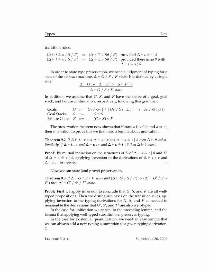
Types L9.9
transition rules.
(∆ ` t.= s / S / F ) ⇒ (∆ ` > / Sθ / F ) provided ∆ ` t
.= s | θ
(∆ ` t.= s / S / F ) ⇒ (∆ ` ⊥ / Sθ / F ) provided there is no θ with
∆ ` t.= s | θ
In order to state type preservation, we need a judgment of typing for astate of the abstract machine, ∆ ` G / S / F state . It is defined by a singlerule.
∆ ` G : o ∆ ` S : o ∆ ` F : o
∆ ` G / S / F state
In addition, we assume that G, S, and F have the shape of a goal, goalstack, and failure continuation, respectively, following this grammar:
Goals G ::= G1 ∧G2 | > | G1 ∨G2 | ⊥ | t.= s | ∃x:τ.G | p(t)
Goal Stacks S ::= > | G ∧ S
Failure Conts F ::= ⊥ | (G ∧ S) ∨ F
The preservation theorem now shows that if state s is valid and s⇒ s′,then s′ is valid. To prove this we first need a lemma about unification.
Theorem 9.2 If ∆ ` t : τ and ∆ ` s : τ and ∆ ` s.= t | θ then ∆ ` θ subst .
Similarly, if ∆ ` t : τ and ∆ ` s : τ and ∆ ` s.= t | θ then ∆ ` θ subst .
Proof: By mutual induction on the structures of D of ∆ ` s.= t | θ and D′
of ∆ ` s.= t | θ, applying inversion to the derivations of ∆ ` t : τ and
∆ ` s : τ as needed. 2
Now we can state (and prove) preservation.
Theorem 9.3 If ∆ ` G / S / F state and (∆ ` G / S / F )⇒ (∆′ ` G′ / S′ /
F ′) then ∆′ ` G′ / S′ / F ′ state .
Proof: First we apply inversion to conclude that G, S, and F are all well-typed propositions. Then we distinguish cases on the transition rules, ap-plying inversion to the typing derivations for G, S, and F as needed toreassemble the derivations that G′, S′, and F ′ are also well-typed.
In the case for unification we appeal to the preceding lemma, and thelemma that applying well-typed substitutions preserves typing.
In the case for existential quantification, we need an easy lemma thatwe can always add a new typing assumption to a given typing derivation.2
LECTURE NOTES SEPTEMBER 26, 2006
L9.10 Types
9.7 The Phase Distinction
While the operational semantics (including unification) preserves types, itdoes not refer to them during execution. In that sense, the types appearingwith quantifiers or the context ∆ are not necessary to execute programs.This means that our type system obeys a so-called phase distinction: we cantype-check our programs, but then execute programs without further ref-erence to types. This is a desirable property since it tells us that there is nocomputational overhead to types at all. On the contrary: types could helpa compiler to optimize the program because it does not have to accountfor the possibility of ill-typed expressions. Types also help us to sort outill-formed expressions, but they do not change the meaning or operationalbehavior of the well-formed ones. Generally, as type systems become moreexpressive, this property is harder to maintain as we will see in the nextlecture.
9.8 Historical Notes
Type systems have a long and rich history, having been developed origi-nally to rule out problems such as Russell’s paradox [3] in the formulationof expressive logics for the formalization of mathematics. Church’s theoryof types [1] provided a great simplification and is also known as classicalhigher-order logic. It uses a type o (omicron) of propositions, a single typeι (iota) for individuals, and closes types under function spaces.
In logic programming, the use of types was slow to arrive since thepredicate calculus (its logical origin) does not usually employ them. Var-ious articles on notion of types in logic programming are available in anedited collection [2].
9.9 Exercises
Exercise 9.1 The notion of type throws a small wrinkle on the soundness andnon-deterministic completeness of an operational semantics with free variables.The new issue is the presence of possibly empty types, either because there are noconstructors, or the constructors are such that no ground terms can be formed.Discuss the issues.
Exercise 9.2 Write out an extension of the system of simple types given herewhich permits Prolog-like overloading of function and predicate symbols at dif-ferent arity. Your extension should continue to satisfy the preservation theorem.
LECTURE NOTES SEPTEMBER 26, 2006
Types L9.11
Exercise 9.3 Write a Prolog program for type checking propositions and terms.Extend your program to type inference where the types on quantifiers are not ex-plicit, generating an explicitly typed proposition (if it is indeed well-typed).
Exercise 9.4 Rewrite the operational rules so that unification is explicitly part ofthe transitions for the abstract machine, rather than a condition.
Exercise 9.5 Show the cases for unification, existential quantification, and atomicgoals in the proof of the type preservation theorem in detail.
Exercise 9.6 Besides type preservation, another important property for a lan-guage is progress: any well-formed state of an abstract machine is either an ex-plicitly characterized final state, or can make a further transition.
In our language, this holds with or without types, if we declare states > / > /
F (for any F ) and ⊥ / S / ⊥ (for any S) final, and assume that G, S, and F
satisfy the grammar for goals, goal stacks and failure continuations shown in thislecture.
Prove the progress theorem.
9.10 References
[1] Alonzo Church. A formulation of the simple theory of types. Journal ofSymbolic Logic, 5:56–68, 1940.
[2] Frank Pfenning, editor. Types in Logic Programming. MIT Press, Cam-bridge, Massachusetts, 1992.
[3] Bertrand Russell. Letter to Frege. In J. van Heijenoort, editor, FromFrege to Godel, pages 124–125. Harvard University Press, 1967. Letterwritten in 1902.
LECTURE NOTES SEPTEMBER 26, 2006

L9.12 Types
LECTURE NOTES SEPTEMBER 26, 2006
15-819K: Logic Programming
Lecture 10
Polymorphism
Frank Pfenning
September 28, 2006
In this lecture we extend the system of simple types from the previous lec-ture to encompass polymorphism. There are some technical pitfalls, andsome plausible systems do not satisfy type preservation. We discuss threeways to restore type preservation.
10.1 Heterogeneous and Homogeneous Lists
Types such as natural numbers, be it in binary or in unary notation, areeasy to specify and use in the system from the previous lecture. Genericdata structures such as lists, on the other hand, present difficulties. Recallthe type predicate for lists:
list([]).
list([X|Xs]) :- list(Xs).
The difficulty is that for lists in general there is no restriction on X: it canhave arbitrary type. When we try to give the declarations
list : type.
[] : list.
’.’ : ?, list -> list.
we realize that there is nothing sensible we can put as the type of the firstargument of cons.1
Two solutions suggest themselves. One is to introduce a universal type“any” and ensure that t : any for all terms t. This destroys the property of
1Recall that [X|Xs] is just alternate syntax for ’.’(X, Xs)
LECTURE NOTES SEPTEMBER 28, 2006
L10.2 Polymorphism
simple types that every well-typed term has a unique type and significantlycomplicates the type system. Following this direction it seems almost in-evitable that some types need to be carried at runtime. A second possibil-ity is to introduce type variables and think of the type of constructors asschematic in their free type variables.
list : type.
[] : list.
’.’ : A, list -> list.
We will pursue this idea in this lecture. Although it is also not withoutproblems, it is quite general and leads to a rich and expressive types sys-tem.
Since the typing rules above are schematic, we get to choose a freshinstance for A every time we use the cons constructor. This means the ele-ments of a list can have arbitrarily different types (they are heterogeneous).
For certain programs it is important to know that the elements of a listall have the same type. For example, we can sort a list of integers, but nota list mixing integers, booleans, and other lists. This requires that list isactually a type constructor: it takes a type as an argument and returns atype. Specifically:
list : type -> type.
[] : list(A).
’.’ : A, list(A) -> list(A).
With these declarations only homogeneous lists will type-check: a term oftype list(A) will be a list all of whose elements are of type A.
10.2 Polymorphic Signatures
We now move to a formal specification of typing. We start with signatures,which now have a more general form. We write α for type variables andα for a sequences of type variables. As in the case of clauses and ordinaryvariables, the official syntax quantifies over type variables in declarations.
Signature Σ ::= · empty signature| Σ, a : type
n→ type type constructor declaration
| Σ, f : ∀α.σ → τ function symbol declaration| Σ, p : ∀α.σ → o predicate symbol declaration
Here, boldface “typen
” stands for a sequence type , . . . , type of lengthn. As usual, if a sequence to the left of the arrow is empty, we may omit
LECTURE NOTES SEPTEMBER 28, 2006
Polymorphism L10.3
the arrow altogether. Similarly, we may omit the quantifier if there are notype variables, and the argument to a type zero-ary types constructor a().Moreover, function and predicate declarations should not contain any freetype variables.
The language of types is also more elaborate, but still does not containfunction types as first-class constructors.
Types τ ::= α | a(τ1, . . . , τn)
10.3 Polymorphic Typing for Terms
The only two rules in the system for simple types that are affected by poly-morphism are those for function and predicate symbols. We account forthe schematic nature of function and predicate declarations by allowing asubstitution θ for the type variables α that occur in the declaration. Wesuppose a fixed signature Σ.
dom(θ) = α
f : ∀α.σ → τ ∈ Σ ∆ ` t : σθ
∆ ` f(t) : τ θ
We use the notation θ to indicate a substitution of types for type variablesrather terms for term variables.
Looking ahead (or back) at the required property of type preservation,one critical lemma is that unification produces a well-typed substitution.Unfortunately, in the presence of polymorphic typing, this property fails!You may want to spend a couple of minutes thinking about a possible coun-terexample before reading on. One way to try to find one (and also a goodstart on fixing the problem) is to attempt a proof and learn from its failure.
False Claim 10.1 If ∆ ` t : τ and ∆ ` s : τ and ∆ ` t.= s | θ then ∆ ` θ subst
and similarly for sequences of terms.
Proof attempt: We proceed by induction on the derivation D of the unifi-cation judgment, applying inversion to the given typing judgments in eachcase. We focus on the problematic one.
Case: D =
D′
∆ ` t.= s | θ
∆ ` f(t).= f(s) | θ
.
LECTURE NOTES SEPTEMBER 28, 2006
L10.4 Polymorphism
We note that we could complete this case if we could appeal to the in-duction hypothesis on D′, since this would yield the well-typednessof θ. We can appeal to the induction hypothesis if we can show that t
and s have the same sequence of types. Let’s see what we can gleanfrom applying inversion to the giving typing derivations. First, wenote that there must be a unique type declaration for f in the signa-ture, say
f : σ → τ ′ ∈ Σ for some σ and τ ′.
Now we write out the inversions on the given typing derivations,using the uniqueness of the declaration for f .
∆ ` f(t) : τ Assumption
τ = τ ′θ1 and ∆ ` t : σθ1 for some θ1 By inversion
∆ ` f(s) : τ Assumption
τ = τ ′θ2 and ∆ ` s : σθ2 for some θ2 By inversion
At this point we would like to conclude
σθ1 = σθ2
because then t and s would have the same sequence of types and wecould finish this case by the induction hypothesis.
Unfortunately, this is not necessarily the case because all we know is
τ = τ ′θ1 = τ ′θ2.
From this we can only onclude that θ1 and θ2 agree on the type vari-ables free in τ ′, but they could differ on variables that occur only in σ
but not in τ ′.
3
From this we can construct a counterexample. Consider heterogeneouslists
nil : list
cons : ∀α.α, list→ list
Thenx:nat ` cons(x, nil) : list
x:nat ` cons(nil, nil) : list
LECTURE NOTES SEPTEMBER 28, 2006
Polymorphism L10.5
and
x:nat ` cons(x, nil).= cons(nil, nil) | (nil/x)
but the returned substitution (nil/x) is not well typed because x:nat andnil:list.
Because unification does not return well-typed substitutions, the oper-ational semantics in whichever form we presented does also not preservetypes. The design of the type system is flawed.
We can pursue two avenues to fix this problem: restricting the typesystem or rewriting the operational semantics.
Type Restriction. In analyzing the failed proof above we can see that atleast this case would go through if we require for a declaration f : ∀α.σ →
τ that every type variable that occurs in σ also occurs in τ . Function sym-bols of this form are called type preserving.2 When all function symbols aretype preserving, the falsely claimed property above actually does hold—the critical case is the one we gave.
Requiring all function symbols to be type preserving rules out hetero-geneous lists, and we need to apply techniques familiar from functionalprogramming to inject elements into a common type. I find this tolerable,but many Prolog programmers would disagree.
Type Passing. We can also modify the operational semantics so that typesare passed and unified at run-time. Then we can use the types to preventthe kind of failure of preservation that arose in the counterexample above.Passing types violates the phase separation and therefore has some over-head. On the other hand, it allows data structures such as heterogeneouslists without additional coding. The language λProlog uses a type passingapproach, together with some optimizations to avoid unnecessary passingof types. We return to this option below.
Before we can make a choice between the two, or resolve the apparentconflict, we must consider the type preservation theorem to make sure weunderstand all the issues.
2Function symbols are constructors, so this is not the same as type preservation in afunctional language. Because of this slightly unfortunate terminology this property hasalso been called transparent.
LECTURE NOTES SEPTEMBER 28, 2006
L10.6 Polymorphism
10.4 Polymorphic Predicates
As it turns out, requiring all function symbols to be type preserving is insuf-ficient to guarantee type preservation. The problem is presented by predi-cate symbols, declared now as p : ∀α.σ → o. If we just unify ∆ ` p(t)
.=
p(s), we run into the same problem as above because predicate symbols arenever type preserving unless they do not have any type variables at all.
Disallowing polymorphic predicates altogether would be too restric-tive, because programs that manipulate generic data structures must bepolymorphic. For example, for homogeneous lists we have
append : list(A), list(A), list(A) -> o.
which is polymorphic in the type variable A.Moreover, the program clauses themselves also need to be polymor-
phic. For example, in the first clause for append
append([], Ys, Ys).
append([X|Xs], Ys, [X|Zs]) :- append(Xs, Ys, Zs).
the variable Ys should be of type list(A) for a type variable A.Before we can solve our problem with type preservation, we must ac-
count for the presence of type variables in program clauses, which nowquantify not only over term variables, but also over type variables. Thegeneral form is ∀α.∀x:σ. p(t) ← G where the type variables α contain allfree type variables in the clause. We will come back to the normal formused in the free variables operational semantics below.
The meaning of universal quantification over types is specified via sub-stitution in the focusing judgment.
Γ;D(τ/α) true ` P true
Γ;∀α.D true ` P true
This just states that an assumption that is schematic in a type variable α
can be instantiated to any type τ . Since logical deduction is ground, weimplicitly assume in the rule above that τ does not contain any free typevariables.
This forces a new typing rule for clauses, which in turn means we haveto slightly generalize contexts to permit declarations α type for type vari-ables.
∆, α type ` A : o
∆ ` ∀α.A : o
LECTURE NOTES SEPTEMBER 28, 2006
Polymorphism L10.7
To be complete and precise, we also need a judgment that types themselvesare well-formed (∆ ` τ type) and similarly for type substitutions (∆ `
θ tsubst); they can be found in various figures at the end of these notes.
p : ∀α.σ → o ∈ Σ
dom(θ) = α
∆ ` θ tsubst ∆ ` t : σθ
∆ ` p(t) : o
Now we reconsider how to solve the problem of polymorphic predi-cates. Looking at the predicate append
append([], Ys, Ys).
append([X|Xs], Ys, [X|Zs]) :- append(Xs, Ys, Zs).
for homogenous lists, we see that no run-time type error can actually arise.This is because the heads of the clauses cover the most general case fora goal. For example, Ys has type list(A) for an arbitrary type A. It cantherefore take on the type of the list in the goal. For example, with a goal
append([], [1,2,3], Zs).
with Zs : list(int), no problem arises because we instantiate the clauseto A = int and then use that instance.
On the other hand, if we added a clause
append([1], [], [1]).
append([], Ys, Ys).
append([X|Xs], Ys, [X|Zs]) :- append(Xs, Ys, Zs).
which is certainly not logically incorrect albeit redundant, then a run-timetype error would occur if we called it with a goal such as
?- append([X], [], Zs), plus(X, s(z), s(s(z))).
where X : nat.What is required is that each clause head for a predicate p is maximally
general or parametric with respect to the declaration of p. More precisely, wesay a clause
∀β.∀x:τ . p(t)← G with p : ∀α.σ → o ∈ Σ
is parametric if there is a type substitution θ with dom(θ) = β with α type `
θ tsubst such thatα type,x:τ θ ` t : σ.
LECTURE NOTES SEPTEMBER 28, 2006

L10.8 Polymorphism
In other words, the types of the arguments t to p in the clause head mustmatch σ in their full generality, keeping all types α fixed.
The proof of type preservation in the presence of this restriction is tech-nically somewhat involved3 so we will omit it here. In the next section wewill see an alternative approach for which type preservation is easy.
10.5 Polymorphic Residuation
When previously describing residuation, we actually were somewhat cav-alier in the treatment of atomic programs (that is, clause heads).
p′(s) ` p(x) > p′(s).= p(x)
Strictly speaking, the resulting equation is not well-formed because it re-lates two atomic propositions rather than two terms. We can eliminate thisinaccuracy by introducing equality between term sequences as a new goalproposition, writing is as t
.= s in overloaded notation. Then we can split
the residuation above into two rules:
p(s) ` p(x) > s.= x
p 6= p′
p(s) ` p′(x) > ⊥
The new pair of rules removes equality between propositions. However,the first rule now has the problem that if p is not maximally general, theresiduated equation s
.= x may not be well-typed!
The idea now is to do some checking during residuation, so that it failswhen a clause head is not maximally general. Since residuation wouldnormally be done statically, as part of compilation of a logic program, wediscover programs that violate the condition at compile time, before theprogram is executed. Following this idea requires passing in a context ∆.to residuation so we can perform type-checking. The two rules above thenbecome
∆ ` x : σ ∆ ` s : σ
∆; p(s) ` p(x) > s.= x
p 6= p′
∆; p(s) ` p′(x) > ⊥
For the program fragment Dp defining p with
p : ∀α.σ → o
3As I am writing these notes, I do not have a complete and detailed proof in the presentcontext.
LECTURE NOTES SEPTEMBER 28, 2006
Polymorphism L10.9
we initially invoke residuation with the most general atomic goal p(x) as in
α type,x:σ;Dp ` p(x) > Gp
leading to the residuated program clause
∀α.∀x:σ. p(x)← Gp.
Residuation is easily extended to handle universally quantified typevariables in programs: we just have to guess how to instantiate them sothat when reaching the head the arguments have the types σ.
∆ ` τ type ∆;D(τ/β) ` p(x) > G
∆;∀β.D ` p(x) > G
Note that this residuation never generates any residual existential quantifi-cation over types. This means that the operational semantics should notallow any free type variables at run-time. This makes sense from a prac-tical perspective: even though programs are generic in the types of datathey can manipulate, when we execute programs they operate on concretedata. Moreoever, since we do not actually carry the types around, their rolewould be quite unclear. Nevertheless, an extension to residuate types thatcannot be guessed at compile-time is possible (see Exercise 10.1).
The operational semantics refers to the residuated program. Since itcontains no equations involving predicates, and we assume all functionsymbols are type preserving, type preservation is now a relatively straight-forward property. The rule for predicate invocation looks as follows:
( p : ∀α.σ → o )( ∆ ` t : σ(τ/α) )∀α.∀x:σ. p(x)← Gp ∆ ` Gp(τ/α)(t/x) / S / F
∆ ` p(t) / S / F
In this rule, formally, we determine a type substitution τ/α, but this isonly a technical device in order to make it easier to state and prove thetype preservation theorem. We have indicated this by parenthesizing theextraneous premisses. During the actual operation of the abstract machine,quantifiers are not annotated with types, and type substitutions are neithercomputed nor applied.
Now type preservation follows in a pretty straightforward way. A crit-ical lemma is parametricity over types4: if α type,∆ ` t : σ then ∆(τ/α) `
4This notion is related to, but not the same as the semantic notion of parametricity infunctional programming.
LECTURE NOTES SEPTEMBER 28, 2006
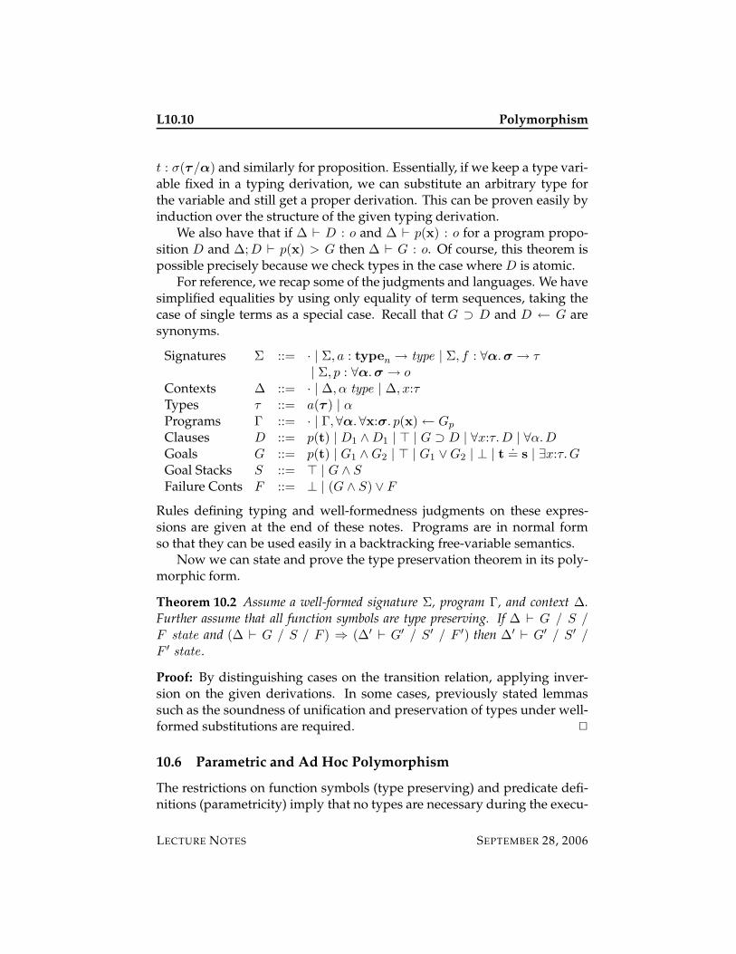
L10.10 Polymorphism
t : σ(τ/α) and similarly for proposition. Essentially, if we keep a type vari-able fixed in a typing derivation, we can substitute an arbitrary type forthe variable and still get a proper derivation. This can be proven easily byinduction over the structure of the given typing derivation.
We also have that if ∆ ` D : o and ∆ ` p(x) : o for a program propo-sition D and ∆;D ` p(x) > G then ∆ ` G : o. Of course, this theorem ispossible precisely because we check types in the case where D is atomic.
For reference, we recap some of the judgments and languages. We havesimplified equalities by using only equality of term sequences, taking thecase of single terms as a special case. Recall that G ⊃ D and D ← G aresynonyms.
Signatures Σ ::= · | Σ, a : typen→ type | Σ, f : ∀α.σ → τ
| Σ, p : ∀α.σ → o
Contexts ∆ ::= · | ∆, α type | ∆, x:τTypes τ ::= a(τ ) | αPrograms Γ ::= · | Γ,∀α.∀x:σ. p(x)← Gp
Clauses D ::= p(t) | D1 ∧D1 | > | G ⊃ D | ∀x:τ.D | ∀α.D
Goals G ::= p(t) | G1 ∧G2 | > | G1 ∨G2 | ⊥ | t.= s | ∃x:τ.G
Goal Stacks S ::= > | G ∧ S
Failure Conts F ::= ⊥ | (G ∧ S) ∨ F
Rules defining typing and well-formedness judgments on these expres-sions are given at the end of these notes. Programs are in normal formso that they can be used easily in a backtracking free-variable semantics.
Now we can state and prove the type preservation theorem in its poly-morphic form.
Theorem 10.2 Assume a well-formed signature Σ, program Γ, and context ∆.Further assume that all function symbols are type preserving. If ∆ ` G / S /
F state and (∆ ` G / S / F ) ⇒ (∆′ ` G′ / S′ / F ′) then ∆′ ` G′ / S′ /
F ′ state .
Proof: By distinguishing cases on the transition relation, applying inver-sion on the given derivations. In some cases, previously stated lemmassuch as the soundness of unification and preservation of types under well-formed substitutions are required. 2
10.6 Parametric and Ad Hoc Polymorphism
The restrictions on function symbols (type preserving) and predicate defi-nitions (parametricity) imply that no types are necessary during the execu-
LECTURE NOTES SEPTEMBER 28, 2006
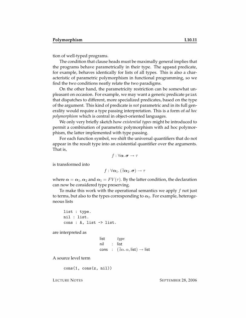
Polymorphism L10.11
tion of well-typed programs.
The condition that clause heads must be maximally general implies thatthe programs behave parametrically in their type. The append predicate,for example, behaves identically for lists of all types. This is also a char-acteristic of parametric polymorphism in functional programming, so wefind the two conditions neatly relate the two paradigms.
On the other hand, the parametricity restriction can be somewhat un-pleasant on occasion. For example, we may want a generic predicate printthat dispatches to different, more specialized predicates, based on the typeof the argument. This kind of predicate is not parametric and in its full gen-erality would require a type passing interpretation. This is a form of ad hocpolymorphism which is central in object-oriented languages.
We only very briefly sketch how existential types might be introduced topermit a combination of parametric polymorphism with ad hoc polymor-phism, the latter implemented with type passing.
For each function symbol, we shift the universal quantifiers that do notappear in the result type into an existential quantifier over the arguments.That is,
f : ∀α.σ → τ
is transformed into
f : ∀α1. (∃α2.σ)→ τ
where α = α1,α2 and α1 = FV (τ). By the latter condition, the declarationcan now be considered type preserving.
To make this work with the operational semantics we apply f not justto terms, but also to the types corresponding to α2. For example, heteroge-neous lists
list : type.
nil : list.
cons : A, list -> list.
are interpreted as
list type
nil : list
cons : (∃α.α, list)→ list
A source level term
cons(1, cons(z, nil))
LECTURE NOTES SEPTEMBER 28, 2006

L10.12 Polymorphism
would be represented as
cons(int; 1, cons(nat; z, nil))
where we use a semi-colon to separate type arguments from term argu-ments. During unification, the type argument as well as the term argu-ments must be unified to guarantee soundness.
For predicates, type parameters that are not treated parametrically mustbe represented as existential quantifiers over the arguments, the parametricones remain universal. For example,
append([1], [], [1]).
append([], Ys, Ys).
append([X|Xs], Ys, [X|Zs]) :- append(Xs, Ys, Zs).
for homogeneous lists is ad hoc polymorphic because of the first clause andshould be given type
append : (∃α. list(α), list(α), list(α))→ o
At least internally, but perhaps even externally, append now has one typeargument and three term arguments.
append(int; [1], [], [1]).
append(A; [], Ys, Ys).
append(A; [X|Xs], Ys, [X|Zs]) :- append(A; Xs, Ys, Zs).
Unification of the type arguments (either implicitly or explicitly) preventsviolation of type preservation, as can be seen from the earlier counterexam-ple
?- append(nat; [X], [], Zs), plus(X, s(z), s(s(z))).
which no fails to match the first clause of append.
The extension of polymorphic typing by using type-passing existentialquantifiers is designed to have the nice property that if the program is para-metric and function symbols are type-preserving, then no types are passedat runtime. However, if function symbols or predicates are needed whichviolate these restrictions, they can be added with some feasible and localoverhead.5
5At the point of this writing this is speculation—I have not seen, formally investigated,or implemented such a system.
LECTURE NOTES SEPTEMBER 28, 2006
Polymorphism L10.13
10.7 Historical Notes
The first proposal for parametrically polymorphic typing in Prolog wasmade by Mycroft and O’Keefe [3] and was strongly influenced by the func-tional language ML. Hanus later refined and extended this proposal [1].Among other things, Hanus considers a type passing interpretation forad hoc polymorphic programs and typed unification. The modern dialectλProlog [2] incorporates polymorphic types and its Teyjus implementationcontains several sophisticated optimizations to handle run-time types effi-ciently [4].
10.8 Exercises
Exercise 10.1 Define an extension of residuation in the presence of polymorphismthat allows free type variable in the body of a clause.
Exercise 10.2 Write out the rules for typing, unification, operational semantics,and sketch type preservation for a type-passing interpretation of existential typesas outlined in this lecture.
Exercise 10.3 Write a type-checker for polymorphic Prolog programs, followingthe starter code and instructions available on the course website.
10.9 References
[1] Michael Hanus. Horn clause programs with polymorphic types: Se-mantics and resolution. Theoretical Computer Science, 89:63–106, 1991.
[2] Dale Miller and Gopalan Nadathur. Higher-order logic programming.In Ehud Shapiro, editor, Proceedings of the Third International Logic Pro-gramming Conference, pages 448–462, London, June 1986.
[3] Alan Mycroft and Richard A. O’Keefe. A polymorphic type system forProlog. Artificial Intelligence, 23(3):295–307, July 1984.
[4] Gopalan Nadathur and Xiaochu Qi. Optimizing the runtime pro-cessing of types in a higher-order logic programming language. InG. Suffcliff and A. Voronkov, editors, Proceedings of the 12th InternationalConference on Logic for Programming, Artificial Intelligence, and Reason-ing (LPAR’05), pages 110–125, Montego Bay, Jamaica, December 2005.Springer LNAI 3835.
LECTURE NOTES SEPTEMBER 28, 2006
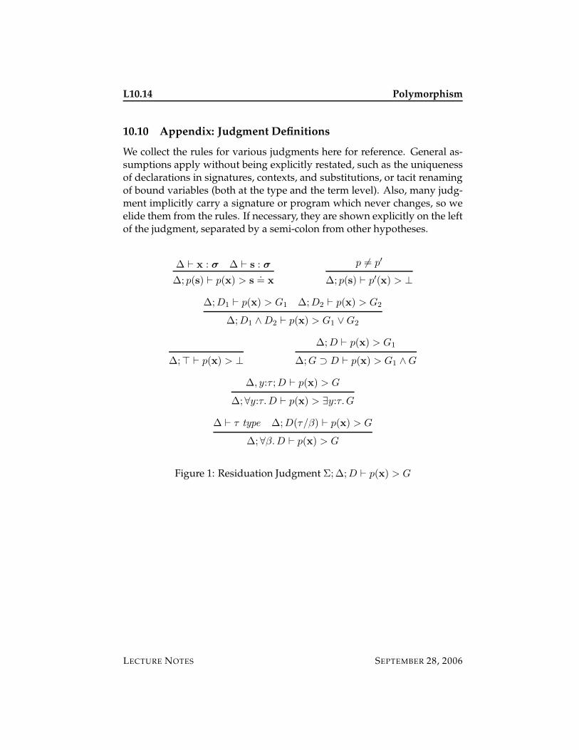
L10.14 Polymorphism
10.10 Appendix: Judgment Definitions
We collect the rules for various judgments here for reference. General as-sumptions apply without being explicitly restated, such as the uniquenessof declarations in signatures, contexts, and substitutions, or tacit renamingof bound variables (both at the type and the term level). Also, many judg-ment implicitly carry a signature or program which never changes, so weelide them from the rules. If necessary, they are shown explicitly on the leftof the judgment, separated by a semi-colon from other hypotheses.
∆ ` x : σ ∆ ` s : σ
∆; p(s) ` p(x) > s.= x
p 6= p′
∆; p(s) ` p′(x) > ⊥
∆;D1 ` p(x) > G1 ∆;D2 ` p(x) > G2
∆;D1 ∧D2 ` p(x) > G1 ∨G2
∆;> ` p(x) > ⊥
∆;D ` p(x) > G1
∆;G ⊃ D ` p(x) > G1 ∧G
∆, y:τ ;D ` p(x) > G
∆;∀y:τ.D ` p(x) > ∃y:τ.G
∆ ` τ type ∆;D(τ/β) ` p(x) > G
∆;∀β.D ` p(x) > G
Figure 1: Residuation Judgment Σ;∆;D ` p(x) > G
LECTURE NOTES SEPTEMBER 28, 2006
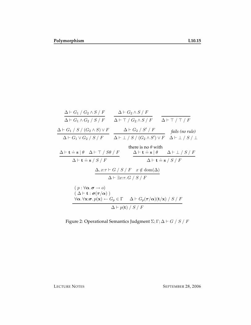
Polymorphism L10.15
∆ ` G1 / G2 ∧ S / F
∆ ` G1 ∧G2 / S / F
∆ ` G2 ∧ S / F
∆ ` > / G2 ∧ S / F ∆ ` > / > / F
∆ ` G1 / S / (G2 ∧ S) ∨ F
∆ ` G1 ∨G2 / S / F
∆ ` G2 / S′ / F
∆ ` ⊥ / S / (G2 ∧ S′) ∨ F
fails (no rule)
∆ ` ⊥ / S / ⊥
∆ ` t.= s | θ ∆ ` > / Sθ / F
∆ ` t.= s / S / F
there is no θ with∆ ` t
.= s | θ ∆ ` ⊥ / S / F
∆ ` t.= s / S / F
∆, x:τ ` G / S / F x /∈ dom(∆)
∆ ` ∃x:τ.G / S / F
( p : ∀α.σ → o)( ∆ ` t : σ(τ/α) )∀α.∀x:σ. p(x)← Gp ∈ Γ ∆ ` Gp(τ/α)(t/x) / S / F
∆ ` p(t) / S / F
Figure 2: Operational Semantics Judgment Σ;Γ;∆ ` G / S / F
LECTURE NOTES SEPTEMBER 28, 2006
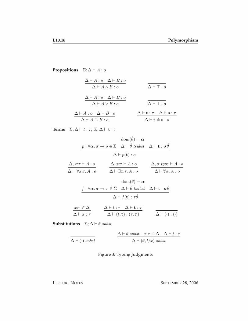
L10.16 Polymorphism
Propositions Σ;∆ ` A : o
∆ ` A : o ∆ ` B : o
∆ ` A ∧B : o ∆ ` > : o
∆ ` A : o ∆ ` B : o
∆ ` A ∨B : o ∆ ` ⊥ : o
∆ ` A : o ∆ ` B : o
∆ ` A ⊃ B : o
∆ ` t : τ ∆ ` s : τ
∆ ` t.= s : o
Terms Σ;∆ ` t : τ, Σ;∆ ` t : τ
p : ∀α.σ → o ∈ Σ
dom(θ) = α
∆ ` θ tsubst ∆ ` t : σθ
∆ ` p(t) : o
∆, x:τ ` A : o
∆ ` ∀x:τ.A : o
∆, x:τ ` A : o
∆ ` ∃x:τ.A : o
∆, α type ` A : o
∆ ` ∀α.A : o
f : ∀α.σ → τ ∈ Σ
dom(θ) = α
∆ ` θ tsubst ∆ ` t : σθ
∆ ` f(t) : τ θ
x:τ ∈ ∆
∆ ` x : τ
∆ ` t : τ ∆ ` t : τ
∆ ` (t, t) : (τ, τ ) ∆ ` (·) : (·)
Substitutions Σ;∆ ` θ subst
∆ ` (·) subst
∆ ` θ subst x:τ ∈ ∆ ∆ ` t : τ
∆ ` (θ, t/x) subst
Figure 3: Typing Judgments
LECTURE NOTES SEPTEMBER 28, 2006
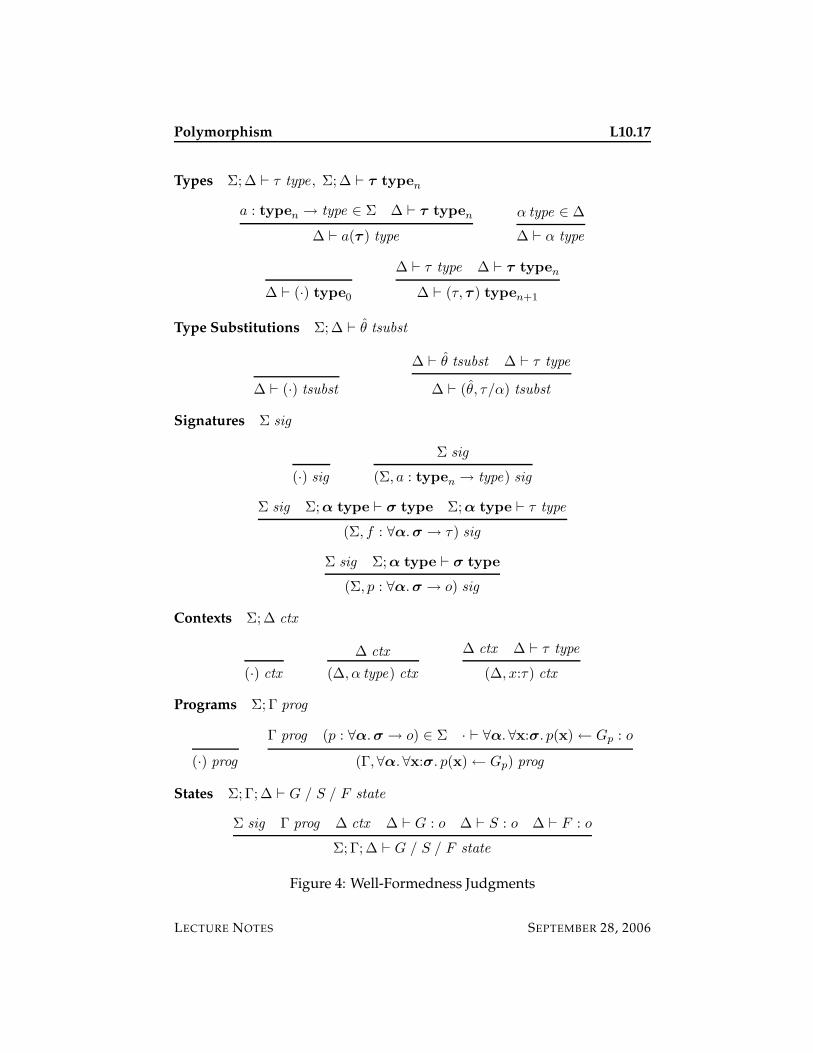
Polymorphism L10.17
Types Σ;∆ ` τ type , Σ;∆ ` τ typen
a : typen→ type ∈ Σ ∆ ` τ type
n
∆ ` a(τ ) type
α type ∈ ∆
∆ ` α type
∆ ` (·) type0
∆ ` τ type ∆ ` τ typen
∆ ` (τ, τ ) typen+1
Type Substitutions Σ;∆ ` θ tsubst
∆ ` (·) tsubst
∆ ` θ tsubst ∆ ` τ type
∆ ` (θ, τ/α) tsubst
Signatures Σ sig
(·) sig
Σ sig
(Σ, a : typen→ type) sig
Σ sig Σ;α type ` σ type Σ;α type ` τ type
(Σ, f : ∀α.σ → τ) sig
Σ sig Σ;α type ` σ type
(Σ, p : ∀α.σ → o) sig
Contexts Σ;∆ ctx
(·) ctx
∆ ctx
(∆, α type) ctx
∆ ctx ∆ ` τ type
(∆, x:τ) ctx
Programs Σ;Γ prog
(·) prog
Γ prog (p : ∀α.σ → o) ∈ Σ · ` ∀α.∀x:σ. p(x)← Gp : o
(Γ,∀α.∀x:σ. p(x)← Gp) prog
States Σ;Γ;∆ ` G / S / F state
Σ sig Γ prog ∆ ctx ∆ ` G : o ∆ ` S : o ∆ ` F : o
Σ;Γ;∆ ` G / S / F state
Figure 4: Well-Formedness Judgments
LECTURE NOTES SEPTEMBER 28, 2006

L10.18 Polymorphism
LECTURE NOTES SEPTEMBER 28, 2006
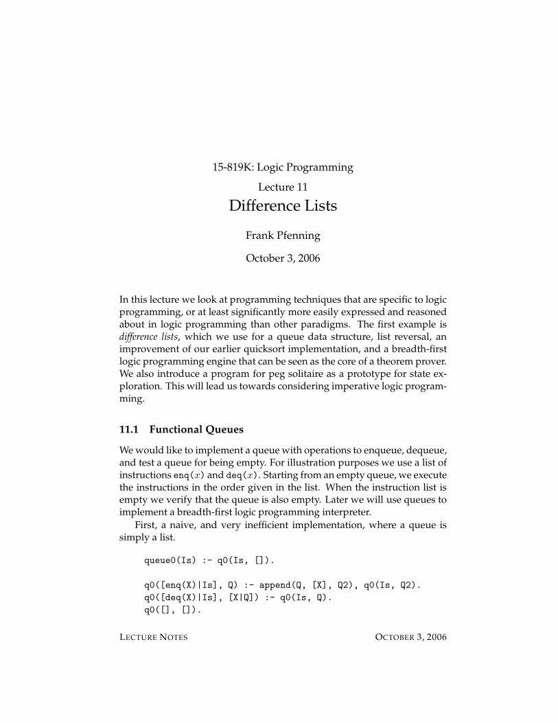
15-819K: Logic Programming
Lecture 11
Difference Lists
Frank Pfenning
October 3, 2006
In this lecture we look at programming techniques that are specific to logicprogramming, or at least significantly more easily expressed and reasonedabout in logic programming than other paradigms. The first example isdifference lists, which we use for a queue data structure, list reversal, animprovement of our earlier quicksort implementation, and a breadth-firstlogic programming engine that can be seen as the core of a theorem prover.We also introduce a program for peg solitaire as a prototype for state ex-ploration. This will lead us towards considering imperative logic program-ming.
11.1 Functional Queues
We would like to implement a queue with operations to enqueue, dequeue,and test a queue for being empty. For illustration purposes we use a list ofinstructions enq(x) and deq(x). Starting from an empty queue, we executethe instructions in the order given in the list. When the instruction list isempty we verify that the queue is also empty. Later we will use queues toimplement a breadth-first logic programming interpreter.
First, a naive, and very inefficient implementation, where a queue issimply a list.
queue0(Is) :- q0(Is, []).
q0([enq(X)|Is], Q) :- append(Q, [X], Q2), q0(Is, Q2).
q0([deq(X)|Is], [X|Q]) :- q0(Is, Q).
q0([], []).
LECTURE NOTES OCTOBER 3, 2006
L11.2 Difference Lists
This is inefficient because of the repeaated calls to append which copy thequeue.
In a more efficient functional implementation we instead maintain twolists, one the front of the list and one the back. We enqueue items on theback and dequeue them from the front. When the front is empty, we reversethe back and make it the new front.
queue1(Is) :- q1(Is, [], []).
q1([enq(X)|Is], F, B) :- q1(Is, F, [X|B]).
q1([deq(X)|Is], [X|F], B) :- q1(Is, F, B).
q1([deq(X)|Is], [], B) :- reverse(B,[X|F]), q1(Is,F,[]).
q1([], [], []).
Depending on the access patterns for queues, this can much more efficientsince the first since the cost of the list reversal can be amortized over theenqueuing and dequeuing operations.
11.2 Queues as Difference Lists
The idea behind this implementation is that the a queue with elementsx1, . . . , xn is represented as a pair [x1, . . ., xn | B] \ B, where B is alogic variable. Here \ is simply a constructor written in infix form to sug-gest list difference because the actual queue of elements for F \ B is the listF minus the tail B.
One may think of the variable B as a pointer to the end of the list, pro-viding a means to add an element at the end in constant time (instead ofcalling append as in the very first implementation). Here is a first imple-mentation using this idea:
queue(Is) :- q(Is, B\B).
q([enq(X)|Is], F\[X|B]) :- q(Is, F\B).
q([deq(X)|Is], [X|F]\B) :- q(Is, F\B).
q([], []\[]).
We consider is line by line, in each case considering the invariant:
A queue x1, . . . , xn is represented by [x1, . . ., xn | B] \ B
for a logic variable B.
In the first clause
LECTURE NOTES OCTOBER 3, 2006
Difference Lists L11.3
queue(Is) :- q(Is, B\B).
we see that the empty queue is represented as B\B for a logic variable B,which is an instance of the invariant for n = 0.
The second clause
q([enq(X)|Is], F\[X|B]) :- q(Is, F\B).
is trickier. A goal matching the head of this clause will have the form
?- q([enq(xn+1)|l], [x1, . . ., xn | B0] \ B0).
for a term xn+1, list l, terms x1, . . . , xn and variable B0. Unification willinstantiate
X = xn+1
Is = l
F = [x1, . . ., xn, xn+1 | B]
B0 = [xn+1 | B]
where B is a fresh logic variable. Now the recursive call is
?- q(l, [x1, . . ., xn, xn+1 | B1] \ B1).
satisfying our representation invariant.The third clause
q([deq(X)|Is], [X|F]\B) :- q(Is, F\B).
looks straightforward, since we are just working on the front of the queue,removing its first element. However, there is a tricky issue when the queueis empty. In that case it has the form B0 \ B0 for some logic variable B0, soit can actually unify with [X|F]. In that case, B0 = [X|F], so the recursivecall will be on q(l, F \ [X|F]) which not only violates our invariant, butalso unexpectedly allows us to remove an element from the empty queue!
The invariant will right itself once we enqueue another element thatmatches X. In other words, we have constructed a “negative” queue, bor-rowing against future elements that have not yet arrived. If this behavioris undesirable, it can be fixed in two ways: we can either add a counter as athird argument that tracks the number of elements in the queue, and thenverify that the counter is positive before dequeuing and element. Or wecan check if the queue is empty before dequeuing and fail explicitly in thatcase.
Let us consider the last clause.
LECTURE NOTES OCTOBER 3, 2006
L11.4 Difference Lists
q([], []\[]).
This checks that the queue is empty by unifying it with []\[]. From theinvariant we can see that it succeeds exactly if the queue is empty (neitherpositive nor negative, if borrowing is allowed).
When we started with the empty queue, we used the phrase B\B for alogic variable B to represent the empty queue. Logically, this is equivalentto checking unifiability with []\[], but operationally this does not workbecause of the lack of occurs-check in Prolog. A non-empty queue such as[x1|B0] \ B0 will incorrectly “unify” with B1\B1 with B1 being instanti-ated to a circular term B1 = [x1|B1].
To complete this example, we show the version that prevents negativequeues by testing if the front is unifiable with [] before proceeding with adequeue operation.
queue(Is) :- q(Is, B\B).
q([enq(X)|Is], F\[X|B]) :- q(Is, F\B).
q([deq(X)|Is], F\B) :-
F = [] -> fail ; F = [X|F1], q(Is, F1\B).
q([], []\[]).
11.3 Other Uses of Difference Lists
In the queue example, it was important that the tail of the list is alwaysa logic variable. There are other uses of difference list where this is notrequired. As a simple example consider reverse. In its naive formulationit overuses append, as in the naive formulation of queues.
naive_reverse([X|Xs], Zs) :-
naive_reverse(Xs, Ys),
append(Ys, [X], Zs).
naive_reverse([], []).
To make this more efficient, we use a difference list as the second argu-ment.
reverse(Xs, Ys) :- rev(Xs, Ys\[]).
rev([X|Xs], Ys\Zs) :- rev(Xs, Ys\[X|Zs]).
rev([], Ys\Ys).
LECTURE NOTES OCTOBER 3, 2006
Difference Lists L11.5
This time, the front of the difference list is a logic variable, to be filled inwhen the input list is empty.
Even though this program is certainly correctly interpreted using listdifference, the use here corresponds straightforwardly to the idea of accu-mulators in functional programming: In rev(Xs, Ys\Zs), Zs accumulatesthe reverse list and eventually returns it in Ys.
Seasoned Prolog hackers will often break up an argument which is adifference list into two top-level arguments for efficiency reasons. So thereverse code above might actually look like
reverse(Xs, Ys) :- rev(Xs, Ys, []).
rev([X|Xs], Ys, Zs) :- rev(Xs, Ys, [X|Zs]).
rev([], Ys, Ys).
where the connection to difference lists is harder to recognize.
Another useful example of difference lists is in quicksort from Lecture2, omitting here the code for partition/4. We construct two lists, Ys1 andYs2 and append them, copying Ys1 again.
quicksort([], []).
quicksort([X0|Xs], Ys) :-
partition(Xs, X0, Ls, Gs),
quicksort(Ls, Ys1),
quicksort(Gs, Ys2),
append(Ys1, [X0|Ys2], Ys).
Instead, we can use a difference list.
quicksort(Xs, Ys) :-
qsort(Xs, Ys\[]).
qsort([], Ys\Ys).
qsort([X0|Xs], Ys\Zs) :-
partition(Xs, X0, Ls, Gs),
qsort(Gs, Ys2\Zs),
qsort(Ls, Ys\[X0|Ys2]).
In this instance of difference lists, it may be helpful to think of
qsort(Xs, Y s\Zs)
LECTURE NOTES OCTOBER 3, 2006
L11.6 Difference Lists
as adding the sorted version of Xs to the front of Zs to obtain Y s. Then,indeed, the result of subtracting Zs from Y s is the sorted version of Xs. Inorder to see this most directly, we have swapped the two recursive calls toqsort so that the tail of the difference list is always ground on invocation.
11.4 A Breadth-First Logic Programming Interpreter
With the ideas of queues outlined above, we can easily construct a breadth-first interpreter for logic programs. Breadth-first search consumes a lot ofspace, and it is very difficult for the programmer to obtain a good modelof program efficiency, so this is best thought of as a naive, first attempt at atheorem prover that can find proofs even where the interpreter would loop.
The code can be found on the course website.1 It is obtained in a prettysimple way from the depth-first interpreter, by replacing the failure contin-uation F by a pair F1\F2, where F2 is always a logic variable that occurs atthe tail of F1. While F1 is not literally a list, it should be easy to see whatthis means.
We show here only four interesting clauses. First three that are directlyconcerned with the failure continuation.
% prove(G, Gamma, S, F1\F2, N, J)
% Gamma |- G / S / FQ, N is next free variable
% J = success or failure
...
prove(bot, _, _, bot\bot, _, J) :- !, J = failure.
prove(bot, Gamma, _, or(and(G2,S),F1)\F2, N, J) :-
prove(G2, Gamma, S, F1\F2, N, J).
prove(or(G1,G2), Gamma, S, F1\or(and(G2,S),F2), N, J) :-
prove(G1, Gamma, S, F1\F2, N, J).
The first clause here needs to commit so that the second clause cannot bor-row against the future. It should match only if there is an element in thequeue.
In order to make this prover complete, we need to cede control imme-diately after an atomic predicate is invoked. Otherwise predicates such as
diverge :- diverge ; true.
would still not terminate since alternatives, even though queued ratherthan stacked, would never be considered. The code for this case looks like
1http://www.cs.cmu.edu/~fp/courses/lp/code/11-diff/meta.pl
LECTURE NOTES OCTOBER 3, 2006
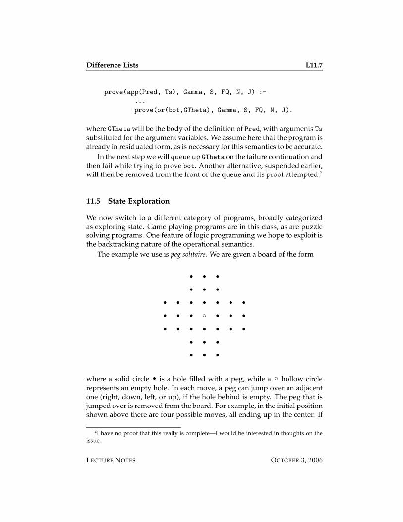
Difference Lists L11.7
prove(app(Pred, Ts), Gamma, S, FQ, N, J) :-
...
prove(or(bot,GTheta), Gamma, S, FQ, N, J).
where GTheta will be the body of the definition of Pred, with arguments Tssubstituted for the argument variables. We assume here that the program isalready in residuated form, as is necessary for this semantics to be accurate.
In the next step we will queue up GTheta on the failure continuation andthen fail while trying to prove bot. Another alternative, suspended earlier,will then be removed from the front of the queue and its proof attempted.2
11.5 State Exploration
We now switch to a different category of programs, broadly categorizedas exploring state. Game playing programs are in this class, as are puzzlesolving programs. One feature of logic programming we hope to exploit isthe backtracking nature of the operational semantics.
The example we use is peg solitaire. We are given a board of the form
s s s
s s s
s s s s s s s
s s s c s s s
s s s s s s s
s s s
s s s
where a solid circle s is a hole filled with a peg, while a c hollow circlerepresents an empty hole. In each move, a peg can jump over an adjacentone (right, down, left, or up), if the hole behind is empty. The peg that isjumped over is removed from the board. For example, in the initial positionshown above there are four possible moves, all ending up in the center. If
2I have no proof that this really is complete—I would be interested in thoughts on theissue.
LECTURE NOTES OCTOBER 3, 2006
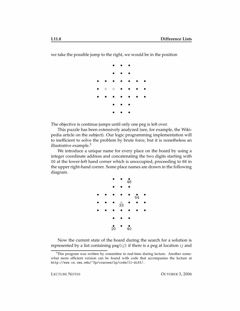
L11.8 Difference Lists
we take the possible jump to the right, we would be in the position
s s s
s s s
s s s s s s s
s c c s s s s
s s s s s s s
s s s
s s s
The objective is continue jumps until only one peg is left over.This puzzle has been extensively analyzed (see, for example, the Wiki-
pedia article on the subject). Our logic programming implementation willto inefficient to solve the problem by brute force, but it is nonetheless anillustrative example.3
We introduce a unique name for every place on the board by using ainteger coordinate address and concatenating the two digits starting with00 at the lower-left hand corner which is unoccupied, proceeding to 66 inthe upper right-hand corner. Some place names are drawn in the followingdiagram.
s s s
s s s
s s s s s s s
s s s c s s s
s s s s s s s
s s s
s s s
20 40
54
46
33
Now the current state of the board during the search for a solution isrepresented by a list containing peg(ij) if there is a peg at location ij and
3This program was written by committee in real-time during lecture. Another some-what more efficient version can be found with code that accompanies the lecture athttp://www.cs.cmu.edu/~fp/courses/lp/code/11-diff/.
LECTURE NOTES OCTOBER 3, 2006
Difference Lists L11.9
hole(ij) if the location ij is an empty hole. We have a prediate init(S0)
which holds for the initial state S0.
init([
peg(20),peg(30),peg(40),
peg(21),peg(31),peg(41),
peg(02),peg(12),peg(22),peg(32),peg(42),peg(52),peg(62),
peg(03),peg(13),peg(23),hole(33),peg(43),peg(53),peg(63),
peg(04),peg(14),peg(24),peg(34),peg(44),peg(54),peg(64),
peg(25),peg(35),peg(45),
peg(26),peg(36),peg(46)
]).
We also have a predicate between/3which holds between three places A, B,and C whenever there is a possible jump to the right or up. This means thatif between(C,B,A) is true then a jump left or up from A to C is possible.We show a few cases in the definition of between.
between(20,30,40).
between(20,21,22).
between(30,31,32).
between(40,41,42).
...
There are 38 such clauses altogether.Next we have a predicate to flip a peg to a hole in a given state returning
the new state.
swap([peg(A)|State], peg(A), [hole(A)|State]).
swap([hole(A)|State], hole(A), [peg(A)|State]).
swap([Place|State1], Place0, [Place|State2]) :-
swap(State1, Place0, State2).
This fails if the requested place is not a peg or hole, respectively.In order to make a single move, we find all candidate triples A, B, or C
using the between relation and then swap the two pegs and hole to be twoholes and a peg.
move1(State1,State4) :-
( between(A,B,C) ; between(C,B,A) ),
swap(State1, peg(A), State2),
swap(State2, peg(B), State3),
swap(State3, hole(C), State4).
LECTURE NOTES OCTOBER 3, 2006
L11.10 Difference Lists
To see if we can make n moves from a given state we make one moveand then see if we can make n − 1 moves from the resulting state. If thisfails, we backtrack, trying another move.
moves(0, _).
moves(N, State1) :-
N > 0,
move1(State1, State2),
N1 is N-1,
moves(N1, State2).
Finally, to solve the puzzle we have to make n moves from the initialstate. To have a full solution, we would need n = 31, since we start with 32pegs so making 31 moves will win.
solve(N) :-
init(State0),
moves(N, State0).
Since in practice we cannot solve the puzzle this way, it is interesting tosee how many sequences of moves of length n are possible from the initialstate. For example, there are 4 possible sequences of a single move and, 12possible sequences of two moves, and 221072 sequences of seven moves.
There we encounter a difficulty, namely that we cannot maintain anyinformation about the number of solutions upon backtracking in pure Pro-log (even though as you have seen in a homework assignments, it is easyto count the number of solutions in the meta-interpreter).
This inability to preserve information is fundamental, so Prolog imple-mentations offer several ways to circumvent it. One class of solutions isrepresented by findall and related predicates which can collect the solu-tions to a query in a list. A second possibility is to use assert and retract
to change the program destructively while it is running—a decidedly non-logical solution. Final, modern Prolog implementations offer global vari-ables that can be assigned to and incremented in a way that survives back-tracking.
We briefly show the third solution in GNU Prolog. A global variable isaddressed by an atom, here count. We can assign to it with g_assign/2,increment it with g_inc/1 and read its value with g_read/2. The idea isto let a call to solve succeed, increment a global variable count, then failand backtrack into solve to find an another solution, etc., until there are nofurther solutions.
LECTURE NOTES OCTOBER 3, 2006
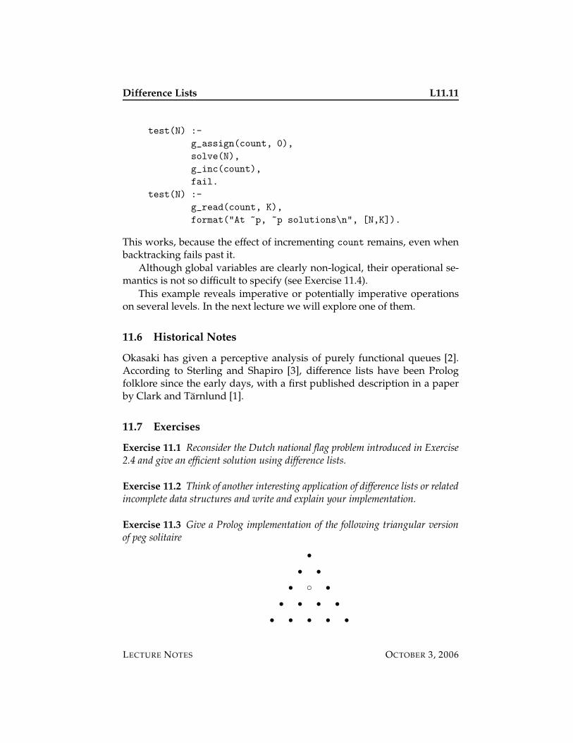
Difference Lists L11.11
test(N) :-
g_assign(count, 0),
solve(N),
g_inc(count),
fail.
test(N) :-
g_read(count, K),
format("At ~p, ~p solutions\n", [N,K]).
This works, because the effect of incrementing count remains, even whenbacktracking fails past it.
Although global variables are clearly non-logical, their operational se-mantics is not so difficult to specify (see Exercise 11.4).
This example reveals imperative or potentially imperative operationson several levels. In the next lecture we will explore one of them.
11.6 Historical Notes
Okasaki has given a perceptive analysis of purely functional queues [2].According to Sterling and Shapiro [3], difference lists have been Prologfolklore since the early days, with a first published description in a paperby Clark and Tarnlund [1].
11.7 Exercises
Exercise 11.1 Reconsider the Dutch national flag problem introduced in Exercise2.4 and give an efficient solution using difference lists.
Exercise 11.2 Think of another interesting application of difference lists or relatedincomplete data structures and write and explain your implementation.
Exercise 11.3 Give a Prolog implementation of the following triangular versionof peg solitaire
s s s s s
s s s s
s c s
s s
s
LECTURE NOTES OCTOBER 3, 2006
L11.12 Difference Lists
where jumps can be made in 6 directions: east, northeast, northwest, west, south-west, and southeast (but not directly north or south). Use your program to de-termine the number of solutions (you may count symmetric ones), and in whichlocations the only remaining peg may end up in. Also, what is the maximal numberof pegs that may be left on the board without any possible further moves?
Exercise 11.4 Give an extension of the operational semantics with goal stacks,failure continuations, and explicit unification to model global variables (named byconstants) which can be assigned, incremented, decremented, and read. Glean theirintended meaning from the use in the test/1 predicate for peg solitaire.
You may assume that the values assigned to global variables in this manner areground and remain unaffected by backtracking.
11.8 References
[1] K. L. Clark and S.-A. Tarnlund. A first order theory of data and pro-grams. In B. Gilchrist, editor, Proceedings of the IFIP Congress, pages939–944, Toronto, Canada, 1977. North Holland.
[2] Chris Okasaki. Simple and efficient purely functional queues and de-ques. Journal of Functional Programming, 5(4):583–592, October 1995.
[3] Leon Sterling and Ehud Shapiro. The Art of Prolog. The MIT Press,Cambridge, Massachusetts, 2nd edition edition, 1994.
LECTURE NOTES OCTOBER 3, 2006
15-819K: Logic Programming
Lecture 12
Linear Logic
Frank Pfenning
October 5, 2006
In this lecture we will rewrite the program for peg solitaire in a way thattreats state logically, rather than as an explicit data structure. In order to al-low this we need to generalize the logic to handle state intrinsically, some-thing provided by linear logic. We provide an introduction to linear logic asa sequent calculus, which generalizes our previous way of specifying truth.The sequent calculus is a bit too general to allow an immediate operationalinterpretation to obtain a logic programming language, so we postpone thisstep to the next lecture.
12.1 State-Passing Style
Let us reexamine the central part of the program for peg solitaire from thelast lecture. The first predicate moves passes state downward in the pro-gram.
moves(0, _).
moves(N, State1) :-
N > 0,
move1(State1, State2),
N1 is N-1,
moves(N1, State2).
The second and third predicates, move1 and swap pass state from an inputargument (the first) to an output argument (the last).
LECTURE NOTES OCTOBER 5, 2006
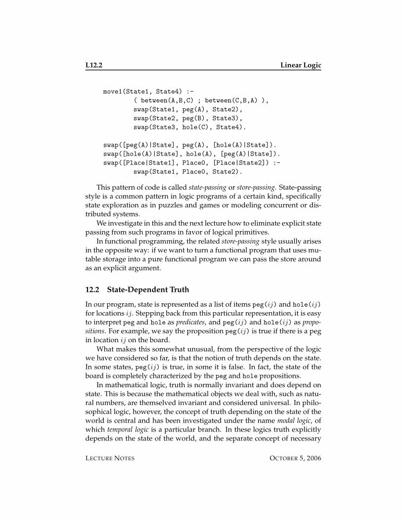
L12.2 Linear Logic
move1(State1, State4) :-
( between(A,B,C) ; between(C,B,A) ),
swap(State1, peg(A), State2),
swap(State2, peg(B), State3),
swap(State3, hole(C), State4).
swap([peg(A)|State], peg(A), [hole(A)|State]).
swap([hole(A)|State], hole(A), [peg(A)|State]).
swap([Place|State1], Place0, [Place|State2]) :-
swap(State1, Place0, State2).
This pattern of code is called state-passing or store-passing. State-passingstyle is a common pattern in logic programs of a certain kind, specificallystate exploration as in puzzles and games or modeling concurrent or dis-tributed systems.
We investigate in this and the next lecture how to eliminate explicit statepassing from such programs in favor of logical primitives.
In functional programming, the related store-passing style usually arisesin the opposite way: if we want to turn a functional program that uses mu-table storage into a pure functional program we can pass the store aroundas an explicit argument.
12.2 State-Dependent Truth
In our program, state is represented as a list of items peg(ij) and hole(ij)
for locations ij. Stepping back from this particular representation, it is easyto interpret peg and hole as predicates, and peg(ij) and hole(ij) as propo-sitions. For example, we say the proposition peg(ij) is true if there is a pegin location ij on the board.
What makes this somewhat unusual, from the perspective of the logicwe have considered so far, is that the notion of truth depends on the state.In some states, peg(ij) is true, in some it is false. In fact, the state of theboard is completely characterized by the peg and hole propositions.
In mathematical logic, truth is normally invariant and does depend onstate. This is because the mathematical objects we deal with, such as natu-ral numbers, are themselved invariant and considered universal. In philo-sophical logic, however, the concept of truth depending on the state of theworld is central and has been investigated under the name modal logic, ofwhich temporal logic is a particular branch. In these logics truth explicitlydepends on the state of the world, and the separate concept of necessary
LECTURE NOTES OCTOBER 5, 2006
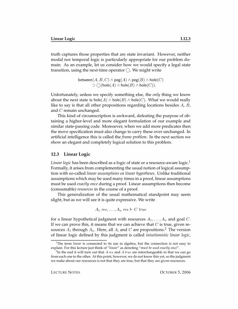
Linear Logic L12.3
truth captures those properties that are state invariant. However, neithermodal nor temporal logic is particularly appropriate for our problem do-main. As an example, let us consider how we would specify a legal statetransition, using the next-time operator ©. We might write
between(A,B,C) ∧ peg(A) ∧ peg(B) ∧ hole(C)⊃ ©(hole(A) ∧ hole(B) ∧ hole(C)).
Unfortunately, unless we specify something else, the only thing we knowabout the next state is hole(A) ∧ hole(B) ∧ hole(C). What we would reallylike to say is that all other propositions regarding locations besides A, B,and C remain unchanged.
This kind of circumscription is awkward, defeating the purpose of ob-taining a higher-level and more elegant formulation of our example andsimilar state-passing code. Moreoever, when we add more predicates thenthe move specification must also change to carry these over unchanged. Inartificial intelligence this is called the frame problem. In the next section weshow an elegant and completely logical solution to this problem.
12.3 Linear Logic
Linear logic has been described as a logic of state or a resource-aware logic.1
Formally, it arises from complementing the usual notion of logical assump-tion with so-called linear assumptions or linear hypotheses. Unlike traditionalassumptions which may be used many times in a proof, linear assumptionsmust be used exactly once during a proof. Linear assumptions then become(consumable) resources in the course of a proof.
This generalization of the usual mathematical standpoint may seemslight, but as we will see it is quite expressive. We write
A1 res , . . . , An res ` C true
for a linear hypothetical judgment with resources A1, . . . , An and goal C .If we can prove this, it means that we can achieve that C is true, given re-sources A1 through An. Here, all Ai and C are propositions.2 The versionof linear logic defined by this judgment is called intuitionistic linear logic,
1The term linear is connected to its use in algebra, but the connection is not easy toexplain. For this lecture just think of “linear” as denoting “must be used exactly once”.
2In the end it will turn out that A res and A true are interchangeable in that we can gofrom each one to the other. At this point, however, we do not know this yet, so the judgmentwe make about our resources is not that they are true, but that they are given resources.
LECTURE NOTES OCTOBER 5, 2006
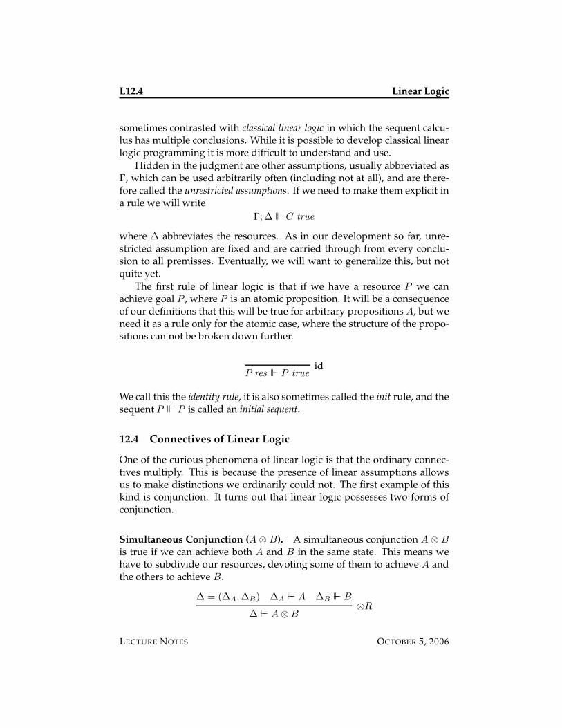
L12.4 Linear Logic
sometimes contrasted with classical linear logic in which the sequent calcu-lus has multiple conclusions. While it is possible to develop classical linearlogic programming it is more difficult to understand and use.
Hidden in the judgment are other assumptions, usually abbreviated asΓ, which can be used arbitrarily often (including not at all), and are there-fore called the unrestricted assumptions. If we need to make them explicit ina rule we will write
Γ;∆ ` C true
where ∆ abbreviates the resources. As in our development so far, unre-stricted assumption are fixed and are carried through from every conclu-sion to all premisses. Eventually, we will want to generalize this, but notquite yet.
The first rule of linear logic is that if we have a resource P we canachieve goal P , where P is an atomic proposition. It will be a consequenceof our definitions that this will be true for arbitrary propositions A, but weneed it as a rule only for the atomic case, where the structure of the propo-sitions can not be broken down further.
P res ` P trueid
We call this the identity rule, it is also sometimes called the init rule, and thesequent P ` P is called an initial sequent.
12.4 Connectives of Linear Logic
One of the curious phenomena of linear logic is that the ordinary connec-tives multiply. This is because the presence of linear assumptions allowsus to make distinctions we ordinarily could not. The first example of thiskind is conjunction. It turns out that linear logic possesses two forms ofconjunction.
Simultaneous Conjunction (A ⊗ B). A simultaneous conjunction A ⊗ B
is true if we can achieve both A and B in the same state. This means wehave to subdivide our resources, devoting some of them to achieve A andthe others to achieve B.
∆ = (∆A,∆B) ∆A ` A ∆B ` B
∆ ` A ⊗ B⊗R
LECTURE NOTES OCTOBER 5, 2006
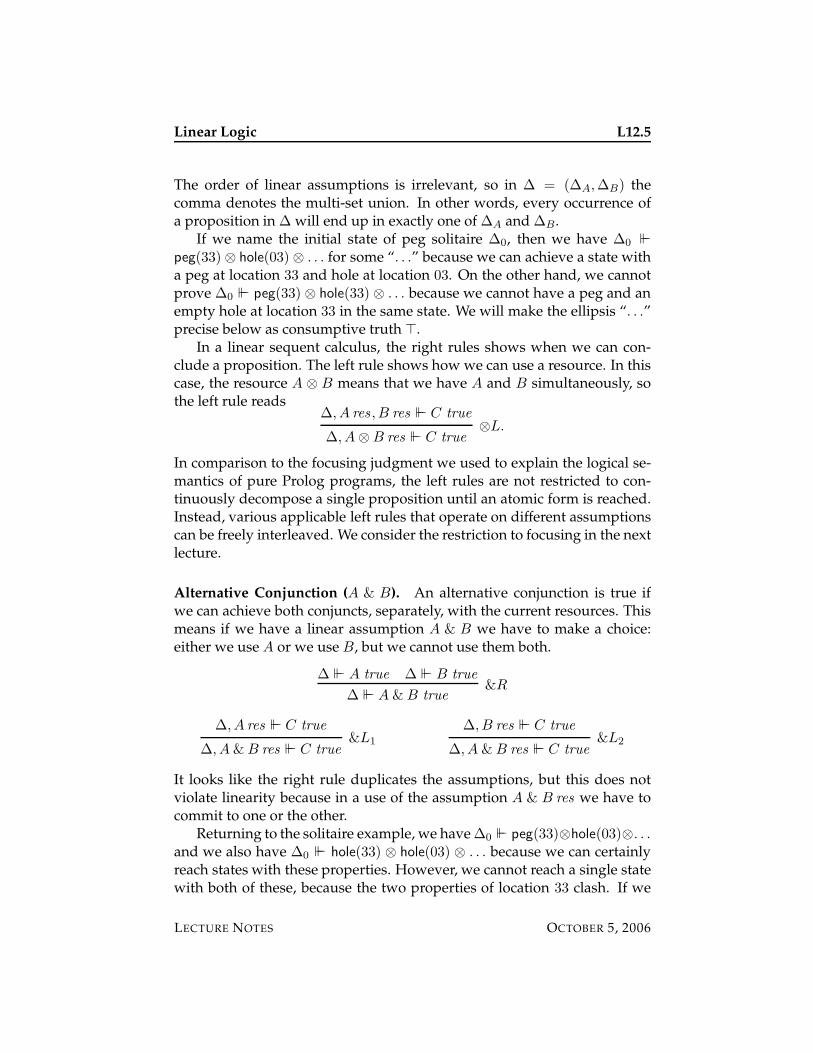
Linear Logic L12.5
The order of linear assumptions is irrelevant, so in ∆ = (∆A,∆B) thecomma denotes the multi-set union. In other words, every occurrence ofa proposition in ∆ will end up in exactly one of ∆A and ∆B.
If we name the initial state of peg solitaire ∆0, then we have ∆0 `
peg(33) ⊗ hole(03) ⊗ . . . for some “. . .” because we can achieve a state witha peg at location 33 and hole at location 03. On the other hand, we cannotprove ∆0 ` peg(33) ⊗ hole(33) ⊗ . . . because we cannot have a peg and anempty hole at location 33 in the same state. We will make the ellipsis “. . .”precise below as consumptive truth >.
In a linear sequent calculus, the right rules shows when we can con-clude a proposition. The left rule shows how we can use a resource. In thiscase, the resource A ⊗ B means that we have A and B simultaneously, sothe left rule reads
∆, A res , B res ` C true
∆, A ⊗ B res ` C true⊗L.
In comparison to the focusing judgment we used to explain the logical se-mantics of pure Prolog programs, the left rules are not restricted to con-tinuously decompose a single proposition until an atomic form is reached.Instead, various applicable left rules that operate on different assumptionscan be freely interleaved. We consider the restriction to focusing in the nextlecture.
Alternative Conjunction (A & B). An alternative conjunction is true ifwe can achieve both conjuncts, separately, with the current resources. Thismeans if we have a linear assumption A & B we have to make a choice:either we use A or we use B, but we cannot use them both.
∆ ` A true ∆ ` B true
∆ ` A & B true&R
∆, A res ` C true
∆, A & B res ` C true&L1
∆, B res ` C true
∆, A & B res ` C true&L2
It looks like the right rule duplicates the assumptions, but this does notviolate linearity because in a use of the assumption A & B res we have tocommit to one or the other.
Returning to the solitaire example, we have ∆0 ` peg(33)⊗hole(03)⊗. . .
and we also have ∆0 ` hole(33) ⊗ hole(03) ⊗ . . . because we can certainlyreach states with these properties. However, we cannot reach a single statewith both of these, because the two properties of location 33 clash. If we
LECTURE NOTES OCTOBER 5, 2006
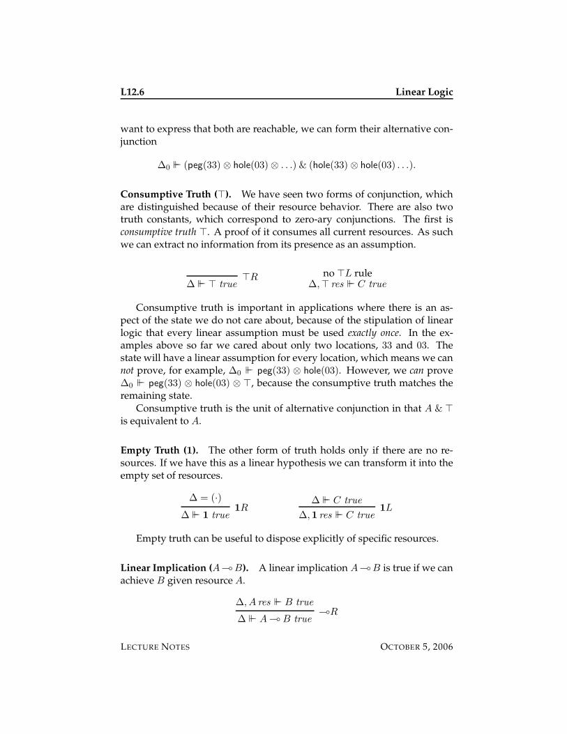
L12.6 Linear Logic
want to express that both are reachable, we can form their alternative con-junction
∆0 ` (peg(33) ⊗ hole(03) ⊗ . . .) & (hole(33) ⊗ hole(03) . . .).
Consumptive Truth (>). We have seen two forms of conjunction, whichare distinguished because of their resource behavior. There are also twotruth constants, which correspond to zero-ary conjunctions. The first isconsumptive truth >. A proof of it consumes all current resources. As suchwe can extract no information from its presence as an assumption.
∆ ` > true>R no >L rule
∆,> res ` C true
Consumptive truth is important in applications where there is an as-pect of the state we do not care about, because of the stipulation of linearlogic that every linear assumption must be used exactly once. In the ex-amples above so far we cared about only two locations, 33 and 03. Thestate will have a linear assumption for every location, which means we cannot prove, for example, ∆0 ` peg(33) ⊗ hole(03). However, we can prove∆0 ` peg(33) ⊗ hole(03) ⊗ >, because the consumptive truth matches theremaining state.
Consumptive truth is the unit of alternative conjunction in that A & >
is equivalent to A.
Empty Truth (1). The other form of truth holds only if there are no re-sources. If we have this as a linear hypothesis we can transform it into theempty set of resources.
∆ = (·)
∆ ` 1 true1R
∆ ` C true
∆,1 res ` C true1L
Empty truth can be useful to dispose explicitly of specific resources.
Linear Implication (A(B). A linear implication A(B is true if we canachieve B given resource A.
∆, A res ` B true
∆ ` A ( B true(R
LECTURE NOTES OCTOBER 5, 2006
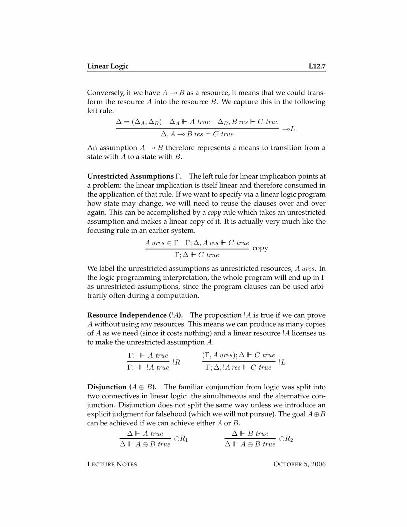
Linear Logic L12.7
Conversely, if we have A ( B as a resource, it means that we could trans-form the resource A into the resource B. We capture this in the followingleft rule:
∆ = (∆A,∆B) ∆A ` A true ∆B, B res ` C true
∆, A ( B res ` C true(L.
An assumption A ( B therefore represents a means to transition from astate with A to a state with B.
Unrestricted Assumptions Γ. The left rule for linear implication points ata problem: the linear implication is itself linear and therefore consumed inthe application of that rule. If we want to specify via a linear logic programhow state may change, we will need to reuse the clauses over and overagain. This can be accomplished by a copy rule which takes an unrestrictedassumption and makes a linear copy of it. It is actually very much like thefocusing rule in an earlier system.
A ures ∈ Γ Γ;∆, A res ` C true
Γ;∆ ` C truecopy
We label the unrestricted assumptions as unrestricted resources, A ures . Inthe logic programming interpretation, the whole program will end up in Γas unrestricted assumptions, since the program clauses can be used arbi-trarily often during a computation.
Resource Independence (!A). The proposition !A is true if we can proveA without using any resources. This means we can produce as many copiesof A as we need (since it costs nothing) and a linear resource !A licenses usto make the unrestricted assumption A.
Γ; · ` A true
Γ; · ` !A true!R
(Γ, A ures);∆ ` C true
Γ;∆, !A res ` C true!L
Disjunction (A ⊕ B). The familiar conjunction from logic was split intotwo connectives in linear logic: the simultaneous and the alternative con-junction. Disjunction does not split the same way unless we introduce anexplicit judgment for falsehood (which we will not pursue). The goal A⊕B
can be achieved if we can achieve either A or B.
∆ ` A true
∆ ` A ⊕ B true⊕R1
∆ ` B true
∆ ` A ⊕ B true⊕R2
LECTURE NOTES OCTOBER 5, 2006
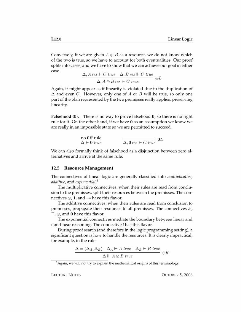
L12.8 Linear Logic
Conversely, if we are given A ⊕ B as a resource, we do not know whichof the two is true, so we have to account for both eventualities. Our proofsplits into cases, and we have to show that we can achieve our goal in eithercase.
∆, A res ` C true ∆, B res ` C true
∆, A ⊕ B res ` C true⊕L
Again, it might appear as if linearity is violated due to the duplication of∆ and even C . However, only one of A or B will be true, so only onepart of the plan represented by the two premisses really applies, preservinglinearity.
Falsehood (0). There is no way to prove falsehood 0, so there is no rightrule for it. On the other hand, if we have 0 as an assumption we know weare really in an impossible state so we are permitted to succeed.
no 0R rule∆ ` 0 true ∆,0 res ` C true
0L
We can also formally think of falsehood as a disjunction between zero al-ternatives and arrive at the same rule.
12.5 Resource Management
The connectives of linear logic are generally classified into multiplicative,additive, and exponential.3
The multiplicative connectives, when their rules are read from conclu-sion to the premisses, split their resources between the premisses. The con-nectives ⊗, 1, and ( have this flavor.
The additive connectives, when their rules are read from conclusion topremisses, propagate their resources to all premisses. The connectives &,>, ⊕, and 0 have this flavor.
The exponential connectives mediate the boundary between linear andnon-linear reasoning. The connective ! has this flavor.
During proof search (and therefore in the logic programming setting), asignificant question is how to handle the resources. It is clearly impractical,for example, in the rule
∆ = (∆A,∆B) ∆A ` A true ∆B ` B true
∆ ` A ⊗ B true⊗R
3Again, we will not try to explain the mathematical origins of this terminology.
LECTURE NOTES OCTOBER 5, 2006
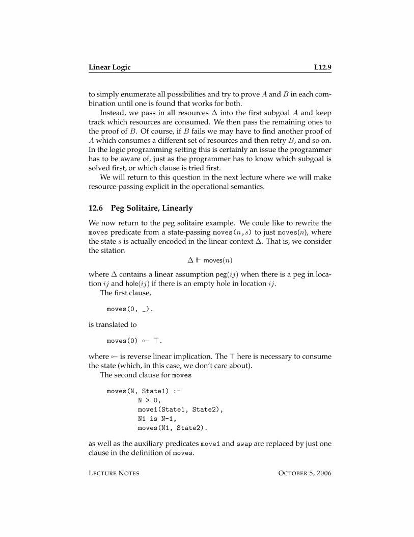
Linear Logic L12.9
to simply enumerate all possibilities and try to prove A and B in each com-bination until one is found that works for both.
Instead, we pass in all resources ∆ into the first subgoal A and keeptrack which resources are consumed. We then pass the remaining ones tothe proof of B. Of course, if B fails we may have to find another proof ofA which consumes a different set of resources and then retry B, and so on.In the logic programming setting this is certainly an issue the programmerhas to be aware of, just as the programmer has to know which subgoal issolved first, or which clause is tried first.
We will return to this question in the next lecture where we will makeresource-passing explicit in the operational semantics.
12.6 Peg Solitaire, Linearly
We now return to the peg solitaire example. We coule like to rewrite themoves predicate from a state-passing moves(n,s) to just moves(n), wherethe state s is actually encoded in the linear context ∆. That is, we considerthe sitation
∆ ` moves(n)
where ∆ contains a linear assumption peg(ij) when there is a peg in loca-tion ij and hole(ij) if there is an empty hole in location ij.
The first clause,
moves(0, _).
is translated to
moves(0) ◦− >.
where ◦− is reverse linear implication. The > here is necessary to consumethe state (which, in this case, we don’t care about).
The second clause for moves
moves(N, State1) :-
N > 0,
move1(State1, State2),
N1 is N-1,
moves(N1, State2).
as well as the auxiliary predicates move1 and swap are replaced by just oneclause in the definition of moves.
LECTURE NOTES OCTOBER 5, 2006
L12.10 Linear Logic
moves(N) ◦−
N > 0 ⊗ N1 is N-1 ⊗
( between(A,B,C) ⊕ between(C,B,A) ) ⊗
peg(A) ⊗ peg(B) ⊗ hole(C) ⊗
(hole(A) ⊗ hole(B) ⊗ peg(C) ( moves(N1)).
Operationally, we first compute n−1 and then find a triple A, B, C such thatB is between A and C . These operations are state independent, althoughthe clause does not indicate that.
At this point we determine if there are pegs at A and B and a hole atC . If this is not the case, we fail and backtrack; if it is we remove thesethree assumptions from the linear context (they are consumed!) and as-sume instead hole(A), hole(B), and peg(C) before calling moves recursivelywith n − 1. At this point this is the only outstanding subgoal, and the statehas changed by jumping A over B into C , as specified.
Observe how linearity and the intrinsic handling of state let’s us replacea lot of code for state management with one short clause.
12.7 Historical Notes
Linear logic in a slightly different form than we present here is due to Gi-rard [2]. He insisted on a classical negation in his formulation, which canget in the way of an elegant logic programming formulation. The judg-mental presentation we use here was developed for several courses on Lin-ear Logic [3] at CMU. Some additional connectives, and some interestingconnections between the two formulations in linear logic are developed byChang, Chaudhuri and Pfenning [1]. We’ll provide some references on lin-ear logic programming in the next lecture.
12.8 Exercises
Exercise 12.1 Prove that A res ` A true for any proposition A.
Exercise 12.2 For each of the following purely linear entailments, give a proofthat they hold or demonstrate that they do not hold because there is no deductionin our system. You do not need to prove formally that no deduction exists.
i. A & (B ⊕ C) ` (A & B) ⊕ (A & C)
ii. A ⊗ (B ⊕ C) ` (A ⊗ B) ⊕ (A ⊗ C)
iii. A ⊕ (B & C) ` (A ⊕ B) & (A ⊕ C)
LECTURE NOTES OCTOBER 5, 2006
Linear Logic L12.11
iv. A ⊕ (B ⊗ C) ` (A ⊕ B) ⊗ (A ⊕ C)
Exercise 12.3 Repeat Exercise 12.2 by checking the reverse linear entailments.
Exercise 12.4 For each of the following purely linear entailments, give a proofthat they hold or demonstrate that they do not hold because there is no deductionin our system. You do not need to prove formally that no deduction exists.
i. A ( (B ( C) ` (A ⊗ B) ( C
ii. (A ⊗ B) ( C ` A ( (B ( C)
iii. A ( (B & C) ` (A ( B) & (A ( C)
iv. (A ( B) & (A ( C) ` A ( (B & C)
v. (A ⊕ B) ( C ` (A ( C) & (A ( C)
vi. (A ( C) & (A ( C) ` (A ⊕ B) ( C
Exercise 12.5 For each of the following purely linear entailments, give a proofthat they hold or demonstrate that they do not hold because there is no deductionin our system. You do not need to prove formally that no deduction exists.
i. C ` 1 ( C
ii. 1 ( C ` C
iii. A ( > ` >
iv. > ` A ( >
v. 0 ( C ` >
vi. > ` 0 ( C
Exercise 12.6 For each of the following purely linear entailments, give a proofthat they hold or demonstrate that they do not hold because there is no deductionin our system. You do not need to prove formally that no deduction exists.
i. !(A ⊗ B) ` !A ⊗ !B
ii. !A ⊗ !B ` !(A ⊗ B)
iii. !(A & B) ` !A ⊗ !B
LECTURE NOTES OCTOBER 5, 2006
L12.12 Linear Logic
iv. !A ⊗ !B ` !(A & B)
v. !> ` 1
vi. 1 ` !>
vii. !1 ` >
viii. > ` !1
ix. !!A ` !A
x. !A ` !!A
12.9 References
[1] Bor-Yuh Evan Chang, Kaustuv Chaudhuri, and Frank Pfenning. Ajudgmental analysis of linear logic. Technical Report CMU-CS-03-131R,Carnegie Mellon University, December 2003.
[2] Jean-Yves Girard. Linear logic. Theoretical Computer Science, 50:1–102,1987.
[3] Frank Pfenning. Linear logic. Lecture Notes for a course at CarnegieMellon University, 1995. Revised 1998, 2001.
12.10 Appendix: Summary of Intuitionistic Linear Logic
In the rules below, we show the unrestricted assumptions Γ only whereaffected by the rule. In all other rules it is propagated unchanged from theconclusion to all the premisses. Also recall that the order of hypotheses isirrelevant, and ∆A,∆B stands for the multiset union of two collections oflinear assumptions.
LECTURE NOTES OCTOBER 5, 2006
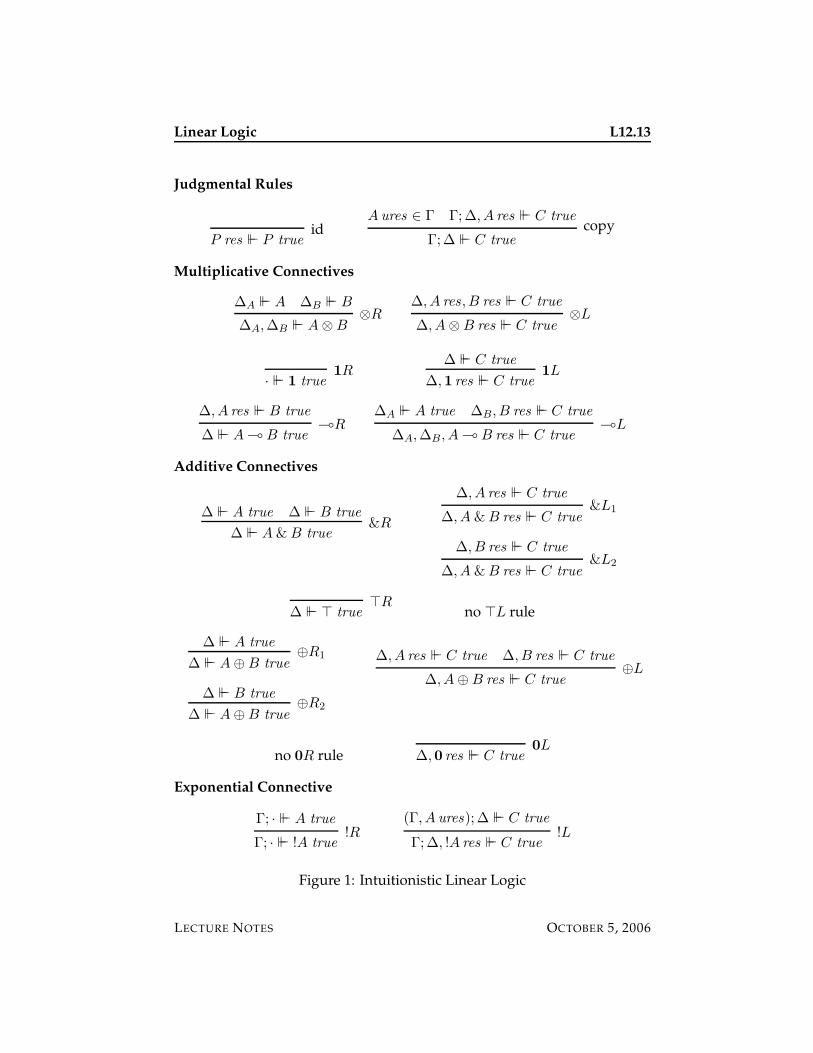
Linear Logic L12.13
Judgmental Rules
P res ` P trueid
A ures ∈ Γ Γ;∆, A res ` C true
Γ;∆ ` C truecopy
Multiplicative Connectives
∆A ` A ∆B ` B
∆A,∆B ` A ⊗ B⊗R
∆, A res , B res ` C true
∆, A ⊗ B res ` C true⊗L
· ` 1 true1R
∆ ` C true
∆,1 res ` C true1L
∆, A res ` B true
∆ ` A ( B true(R
∆A ` A true ∆B, B res ` C true
∆A,∆B , A ( B res ` C true(L
Additive Connectives
∆ ` A true ∆ ` B true
∆ ` A & B true&R
∆, A res ` C true
∆, A & B res ` C true&L1
∆, B res ` C true
∆, A & B res ` C true&L2
∆ ` > true>R
no >L rule
∆ ` A true
∆ ` A ⊕ B true⊕R1
∆ ` B true
∆ ` A ⊕ B true⊕R2
∆, A res ` C true ∆, B res ` C true
∆, A ⊕ B res ` C true⊕L
no 0R rule ∆,0 res ` C true0L
Exponential Connective
Γ; · ` A true
Γ; · ` !A true!R
(Γ, A ures);∆ ` C true
Γ;∆, !A res ` C true!L
Figure 1: Intuitionistic Linear Logic
LECTURE NOTES OCTOBER 5, 2006

L12.14 Linear Logic
LECTURE NOTES OCTOBER 5, 2006
15-819K: Logic Programming
Lecture 13
Abstract Logic Programming
Frank Pfenning
October 10, 2006
In this lecture we discuss general criteria to judge whether a logic or a frag-ment of it can be considered a logic programming language. Taking suchcriteria as absolute is counterproductive, but they might nonetheless pro-vide some useful insight in the design of richer languages. Three criteriaemerge: the first two characterize the relationship to logic in that the lan-guage should be sound and (non-deterministically) complete, allowing usto interpret both success and finite failure. The third is operational: wewould like to be able to interpret connectives in goals as search instruc-tions, giving them a predictable operational semantics.
13.1 Logic and Logic Programming
For a language to claim to be a logic programming language, the first cri-terion seems to be soundness with respect to the logical interpretation ofthe program. I consider this non-negotiable: when the interpreter claimssomething is true, it should be true. Otherwise, it may be a programminglanguage, but the connection to logic has been lost. Prolog, unfortunately,is unsound in this respect, due to the lack of occurs-check and the incorrecttreatment of disequality. We either have to hope or verify that these featuresof Prolog did not interfere with the correctness of the answer. Other non-logical features such as meta-call, cut, or input and output are borderlinewith respect to this criterion: since these do not have a logical interpreta-tion, it is difficult to assess soundness of such programs, except by referenceto an operational semantics.
The second criterion is non-deterministic completeness. This meansthat if search fails finitely, no proof can exist. This does not seem quite
LECTURE NOTES OCTOBER 10, 2006
L13.2 Abstract Logic Programming
as fundamental, since we should be mostly interested in obtaining proofswhen they exist, but from an abstract perspective it is certainly desirable.Again, this fails for full Prolog, but is satisfied by pure Prolog even with adepth-first interpreter.
Summary: if we would like to abstractly classify logics or logical frag-ments as suitable basis for logic programming languages, we would expectat least soundness and non-deterministic completeness so we can correctlyinterpret success and failure of goals.
13.2 Logic Programming as Goal-Directed Search
Soundness and completeness (in some form) establish a connection to logic,but by themselves they are clearly insufficient from a programming per-spective. For example, a general purpose theorem prover for a logic issound and complete, and yet not by itself useful for programming. Wewould like to ensure, for example, that our implementation of quicksortreally is an implementation of quicksort, and similarly for mergesort. Theprogrammer should be able to predict and control operational behaviorwell enough to cast algorithms into correct implementations.
As we have seen in the case of Prolog, if the language of goals is suffi-ciently rich, we can transform all the clauses defining a predicate into theform ∀x. p(x) ← G through a process of residuation. Searching for a proofof a goal p(t) then becomes a procedure call, solving instead G(t/x), whichis another goal. In that way, all computational mechanisms are concen-trated on the interpretation of goals. Logic programming, as conceived sofar, is goal-directed search. Elevating these observations to a design princi-ple we postulate:
An abstract logic programming language is defined by a subsetof the propositions in a logic together with an operational semanticsvia proof search on that subset. The operational semantics should besound, non-deterministically complete, and goal-directed.
But what exactly does goal-directed search mean? If we consider a se-quent . . . ` G true where “. . .” collects all hypotheses (linear, unrestricted,and whatever judgments may arise in other logics), then search is goal-directed if we can always break down the structure of the goal G first beforeconsidering the hypotheses, including the program. This leads us to thedefinition of asynchronous connectives.
LECTURE NOTES OCTOBER 10, 2006
Abstract Logic Programming L13.3
13.3 Asynchronous Connectives
A logial constant or connective is asynchronous if its right rule can alwaysbe applied eagerly without loosing completeness. For example, A & B isasynchronous, because the rule
∆ ` A true ∆ ` B true
∆ ` A & B true&R
can always be used for a conjunctive goal A & B, rather than first applyinga left rule to an assumption ∆ or the using a clause in the program Γ. Thisintuitively coincides with our reading of conjunction as a search instruc-tions: to search for a proof of A & B, first find a proof of A and then of B.This does not talk about possibly having to decompose the program. Theproperty of being asynchronous turns out to be relatively easy to prove.For example, given ∆ ` A & B true , we can prove that ∆ ` A true and∆ ` B true by induction on the structure of the given derivation.
On the other hand, the disjunction A⊕B (which corresponds to A ∨B
in ordinary logic programming) is not asynchronous. As a countexample,consider
C,C ( (B ⊕A) ` A⊕B.
We can use neither the ⊕R1 nor the ⊕R2 rule, because neither
C,C ( (B ⊕A) ` A
norC,C ( (B ⊕A) ` B
are provable. Instead we can prove it as follows in the sequent calculus:
C ` Cid
B ` Bid
B ` A⊕B⊕R2
A ` Aid
A ` A⊕B⊕R1
B ⊕A ` A⊕B⊕L
C,C ( (B ⊕A) ` A⊕B(L.
Observe that we took two steps on the left ((L and ⊕L) before decompos-ing the right.
This counterexample shows that we could not decompose A⊕B eagerlyin goal-directed search, unless we are willing to sacrifice completeness. Butwhat, then, would the program C,C ( (B ⊕A) mean?
LECTURE NOTES OCTOBER 10, 2006
L13.4 Abstract Logic Programming
We have already seen that disjunction is useful in Prolog programs, andthe same is true for linear logic programs, so this would seem unfortunate.Before we rescue disjunction, let us analyze which connectives are asyn-chronous.
We postpone the proofs that the asynchronous connectives are indeedasynchronous, and just give counterexamples for those that are not asyn-chronous.
C,C ( (B ⊗A) ` A⊗B
C,C ( 1 ` 1
C,C ( (B ⊕A) ` A⊕B
C,C ( 0 ` 0
C,C ( !A ` !A
In each case we have to apply two left rules first, before any right rule canbe applied.
This leaves A(B, A&B, and> as asynchronous. Atomic propositionshave a somewhat special status in that we cannot decompose them, but wehave to switch to the left-hand side and focus on an assumption (whichmodels procedure call).
We have not discussed the rules for linear quantifiers (see below) but itturns out that ∀x.A is asynchronous, while ∃x.A is not asynchronous.
13.4 Asynchronous Connectives vs. Invertibility of Rules
We call an inference rules invertible if the premisses are provable wheneverthe conclusion is. It is tempting to think that a connective is asynchronousif and only if its right rule is invertible. Not so. Please consider the questionand see a counterexample at the end of the lecture notes only in despara-tion.
13.5 Unrestricted Implication
The analysis so far would suggest that the fragment of our logic has theform
A ::= P | A1 ( A2 | A1 & A2 | > | ∀x.A
However, this is insufficient, because it is purely linear. Usually we inte-grate non-linear reasoning into linear logic using the “of course” operator‘!’, but this is not asynchronous. Instead we can use ordinary implicationto complete the picture. The proposition A ⊃ B is true if assuming A as an
LECTURE NOTES OCTOBER 10, 2006
Abstract Logic Programming L13.5
unrestricted resource we can prove B.
Γ, A ures ;∆ ` B true
Γ;∆ ` A ⊃ B true⊃R
Γ; · ` A true Γ;∆ ` C true
Γ;∆, A ⊃ B res ` C true⊃L
In the left rule for implication, we cannot use any linear resources to proveA, because A may be used in an unrestricted way when proving B. Wewould need those resources potentially many times in the proof of B, vio-lating linearity of the overall system.
The implication A ⊃ B is equivalent to (!A)(B (see Exercise 13.1), butthey have different proof theoretic properties since !A is not asynchronous.
13.6 Focusing and Synchronous Connectives
If all goal connectives are asynchronous, then we will hit eventually hitan atomic predicate without even looking at the program. What happensthen? Recall from Lecture 8 that we now focus on a particular programclause and decompose this in a focusing phase. In the setting here this justmeans that the left rules are applied in sequence to the proposition in focusuntil an atomic formula is reached, and this formula then must match theconclusion.
In general, we call a connective synchronous if we can continue to fo-cus on its components when it is in focus without losing completeness.Note that in logic programming we focus on assumptions (that is, programclauses or part of the state), so the status of a connective as synchronousor asynchronous has be considered separately depending on whether it oc-curs as a goal (on the right-hand side) or as an assumption (on the left-handside). A remarkable fact is that all the connectives that were asynchronousas goals are synchronous as assumptions.
We now write ∆;A � P for a focus on A where we just wrote ∆;A `P earlier, to avoid potential confusion with other hypothetical judgmentforms.
Unlike the decomposition of asynchronous connectives (which is com-pletely mechanical), the decomposition of propositions in focus in the syn-chronous phase of search involves choices. For example the pair of rules
∆;A1 res � P true
∆;A1 ∧A2 res � P true&L1
∆;A2 res � P true
∆;A1 ∧A2 res � P true&L2
requires a choice between A1 and A2 in the focusing phase of search, andsimilarly for other connectives.
LECTURE NOTES OCTOBER 10, 2006
L13.6 Abstract Logic Programming
To restate the focusing property again: it allows us to continue to makechoices on the proposition in focus, without reconsidering other assump-tions, until we reach an atomic proposition. If that matches the conclusionthat branch of the proof succeeds, otherwise it fails.
In the next lecture we will get a hint on how to prove this, although wewill not do this in full detail.
We close this section by giving the focusing rules for the asynchronousfragment of linear logic, which is at the heart of our logic programming lan-guage. The rules can be found in Figure 1. Unfortunately our motivatingexample from the earlier lecture does not fall into this fragment. For exam-ple, we used both simultaneous conjunction A ⊗ B and disjunction A ⊕ B
as goals which are so far prohibit. We will resurrect them via residuation,not because they truly add expressive power, but they are convenient bothfor program expression and for compilation.
13.7 Historical Notes
The notion that a logic programming language should be characterizedas a fragment of logic with complete goal-directed search originated withMiller, Nadathur, and Scedrov [11] who explored logic programming basedon higher-order logic. A revised and expanded version appeared a coupleof years later [10]. These papers introduced the term uniform proofs for thoseproofs that work asynchronously on the goal until it is atomic.
Some time later this was generalized by Andreoli and Pareschi who firstrecognized the potential of linear logic for logic programming [3]. Theyused a fragment of classical linear logic (rather than the intuitionistic linearlogic we use here), which does not have a distinguished notion of goal. Thelanguage LO was therefore more suited to concurrent and object-orientedprogramming [1, 5, 4].
Andreoli also generalized the earlier notion of uniform proofs to focus-ing proofs [2], capturing now both the asynchronous as well as the syn-chronous behavior of connectives in a proof-theoretic manner. This seminalwork subsequently had many important applications in logic, concurrency,and functional programming, and not just in logic programming.
The thread of research on intuitionistic, goal-directed logic program-ming resumed with the work by Hodas and Miller [8, 9] who proposedessentially what we presented in this lecture, with some additional extra-logical features borrowed from Prolog. In honor of its central new con-nective the language was called Lolli. These ideas were later picked up inthe design of a linear logical framework [6, 7] which augments Lolli with a
LECTURE NOTES OCTOBER 10, 2006
Abstract Logic Programming L13.7
richer quantification and explicit proof terms.
13.8 Exercises
Exercise 13.1 Prove that A ⊃ B is equivalent to (!A) ( B in the sense that eachentails the other, that is, A ⊃ B ` (!A) ( B and vice versa.
Exercise 13.2 At one point we defined pure Prolog with the connectives A ∧ B,>, A∨B,⊥, A ⊃ B, and ∀x.A, suitably restricted into legal goals and programs.Show how to translate such programs and goals into linear logic so that focusingproofs for (non-linear) logic are mapped isomorphically to focusing proofs in linearlogic, and prove that your translation is correct in that sense.
13.9 Answer
Consider the right rule for !A.
Γ; · ` A true
Γ; · ` !A true!R
This rule is invertible: whenever the conclusion is provable, then so is thepremiss. However, !A is not asynchronous (see the counterexample in thislecture). If we had formulated the rule as
∆ = (·) Γ; · ` A true
Γ;∆ ` !A true!R
we would have recognized it as not being invertible, because ∆ is not nec-essarily empty.
13.10 References
[1] Jean-Marc Andreoli. Proposal for a Synthesis of Logic and Object-OrientedProgramming Paradigms. PhD thesis, University of Paris VI, 1990.
[2] Jean-Marc Andreoli. Logic programming with focusing proofs in lin-ear logic. Journal of Logic and Computation, 2(3):297–347, 1992.
[3] Jean-Marc Andreoli and Remo Pareschi. LO and behold! Concurrentstructured processes. In Proceedings of OOPSLA’90, pages 44–56, Ot-tawa, Canada, October 1990. Published as ACM SIGPLAN Notices,vol.25, no.10.
LECTURE NOTES OCTOBER 10, 2006
L13.8 Abstract Logic Programming
[4] Jean-Marc Andreoli and Remo Pareschi. Linear objects: Logical pro-cesses with built-in inheritance. New Generation Computing, 9:445–473,1991.
[5] Jean-Marc Andreoli and Remo Pareschi. Logic programming with se-quent systems: A linear logic approach. In P. Schroder-Heister, editor,Proceedings of Workshop to Extensions of Logic Programming, Tubingen,1989, pages 1–30. Springer-Verlag LNAI 475, 1991.
[6] Iliano Cervesato and Frank Pfenning. A linear logical framework. InE. Clarke, editor, Proceedings of the Eleventh Annual Symposium on Logicin Computer Science, pages 264–275, New Brunswick, New Jersey, July1996. IEEE Computer Society Press.
[7] Iliano Cervesato and Frank Pfenning. A linear logical framework. In-formation & Computation, 179(1):19–75, November 2002.
[8] Joshua S. Hodas and Dale Miller. Logic programming in a fragmentof intuitionistic linear logic. In Proceedings of the 6th Annual Symposiumon Logic in Computer Science (LICS’91), pages 32–42, Amsterdam, TheNetherlands, July 1991. IEEE Computer Society Press.
[9] Joshua S. Hodas and Dale Miller. Logic programming in a fragment ofintuitionistic linear logic. Information and Computation, 110(2):327–365,1994.
[10] Dale Miller, Gopalan Nadathur, Frank Pfenning, and Andre Scedrov.Uniform proofs as a foundation for logic programming. Annals of Pureand Applied Logic, 51:125–157, 1991.
[11] Dale Miller, Gopalan Nadathur, and Andre Scedrov. Hereditary Har-rop formulas and uniform proof systems. In David Gries, editor, Sym-posium on Logic in Computer Science, pages 98–105, Ithaca, NY, June1987.
LECTURE NOTES OCTOBER 10, 2006

Abstract Logic Programming L13.9
Judgmental Rules
P res � P trueid
A ures ∈ Γ Γ;∆;A res � P true
Γ;∆ ` P truecopy
∆;A res � P true
∆, A res ` P truefocus
Multiplicative Connective
∆, A res ` B true
∆ ` A ( B true(R
∆A ` A true ∆B;B res � P true
∆A,∆B ;A ( B res � P true(L
Additive Connectives
∆ ` A true ∆ ` B true
∆ ` A & B true&R
∆;A res � P true
∆;A & B res � P true&L1
∆;B res � P true
∆;A & B res � P true&L2
∆ ` > true>R
no >L rule
Exponential Connective
(Γ, A ures);∆ ` B true
Γ;∆ ` A ⊃ B true⊃R
Γ; · ` A true Γ;B res � P true
Γ;∆;A ⊃ B res � P true⊃L
Quantifier
∆ ` A x /∈ FV(Γ;∆)
∆ ` ∀x.A∀R
∆;A(t/x) res � P true
∆;∀x.A res � P true∀L
Figure 1: Focused Intuitionistic Linear Logic; Asynchronous Fragment
LECTURE NOTES OCTOBER 10, 2006

L13.10 Abstract Logic Programming
LECTURE NOTES OCTOBER 10, 2006
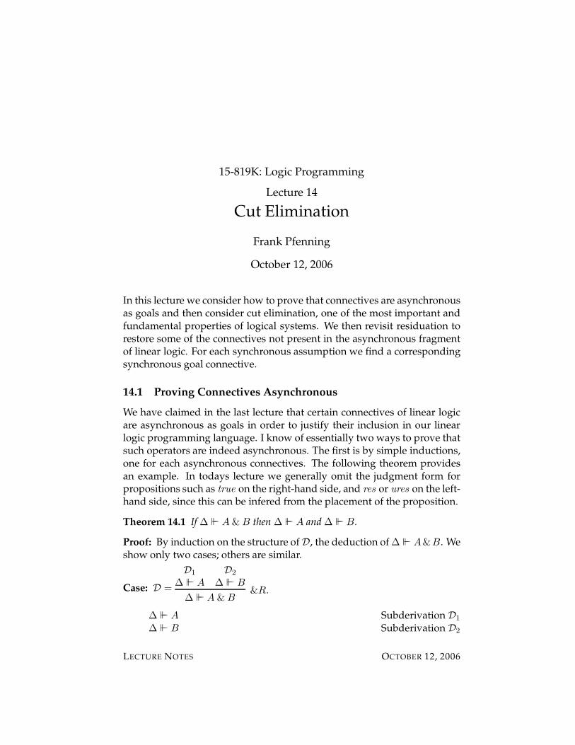
15-819K: Logic Programming
Lecture 14
Cut Elimination
Frank Pfenning
October 12, 2006
In this lecture we consider how to prove that connectives are asynchronousas goals and then consider cut elimination, one of the most important andfundamental properties of logical systems. We then revisit residuation torestore some of the connectives not present in the asynchronous fragmentof linear logic. For each synchronous assumption we find a correspondingsynchronous goal connective.
14.1 Proving Connectives Asynchronous
We have claimed in the last lecture that certain connectives of linear logicare asynchronous as goals in order to justify their inclusion in our linearlogic programming language. I know of essentially two ways to prove thatsuch operators are indeed asynchronous. The first is by simple inductions,one for each asynchronous connectives. The following theorem providesan example. In todays lecture we generally omit the judgment form forpropositions such as true on the right-hand side, and res or ures on the left-hand side, since this can be infered from the placement of the proposition.
Theorem 14.1 If ∆ ` A & B then ∆ ` A and ∆ ` B.
Proof: By induction on the structure of D, the deduction of ∆ ` A&B. Weshow only two cases; others are similar.
Case: D =
D1
∆ ` A
D2
∆ ` B
∆ ` A & B&R.
∆ ` A Subderivation D1
∆ ` B Subderivation D2
LECTURE NOTES OCTOBER 12, 2006
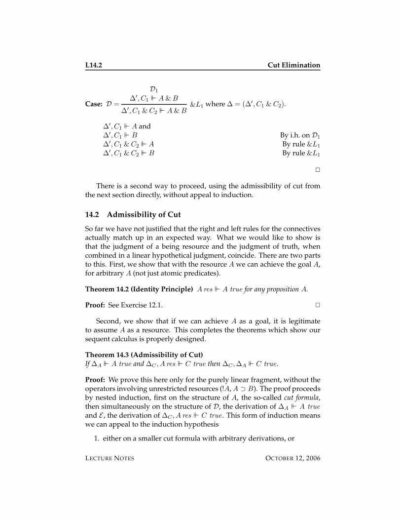
L14.2 Cut Elimination
Case: D =
D1
∆′, C1 ` A & B
∆′, C1 & C2 ` A & B&L1 where ∆ = (∆′, C1 & C2).
∆′, C1 ` A and∆′, C1 ` B By i.h. on D1
∆′, C1 & C2 ` A By rule &L1
∆′, C1 & C2 ` B By rule &L1
2
There is a second way to proceed, using the admissibility of cut fromthe next section directly, without appeal to induction.
14.2 Admissibility of Cut
So far we have not justified that the right and left rules for the connectivesactually match up in an expected way. What we would like to show isthat the judgment of a being resource and the judgment of truth, whencombined in a linear hypothetical judgment, coincide. There are two partsto this. First, we show that with the resource A we can achieve the goal A,for arbitrary A (not just atomic predicates).
Theorem 14.2 (Identity Principle) A res ` A true for any proposition A.
Proof: See Exercise 12.1. 2
Second, we show that if we can achieve A as a goal, it is legitimateto assume A as a resource. This completes the theorems which show oursequent calculus is properly designed.
Theorem 14.3 (Admissibility of Cut)
If ∆A ` A true and ∆C , A res ` C true then ∆C ,∆A ` C true .
Proof: We prove this here only for the purely linear fragment, without theoperators involving unrestricted resources (!A, A ⊃ B). The proof proceedsby nested induction, first on the structure of A, the so-called cut formula,then simultaneously on the structure of D, the derivation of ∆A ` A true
and E , the derivation of ∆C , A res ` C true . This form of induction meanswe can appeal to the induction hypothesis
1. either on a smaller cut formula with arbitrary derivations, or
LECTURE NOTES OCTOBER 12, 2006
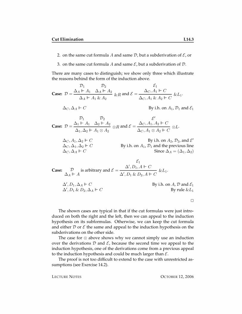
Cut Elimination L14.3
2. on the same cut formula A and same D, but a subderivation of E , or
3. on the same cut formula A and same E , but a subderivation of D.
There are many cases to distinguish; we show only three which illustratethe reasons behind the form of the induction above.
Case: D =
D1
∆A ` A1
D2
∆A ` A2
∆A ` A1 & A2
&R and E =
E1
∆C , A1 ` C
∆C , A1 & A2 ` C&L1
.
∆C ,∆A ` C By i.h. on A1, D1 and E1
Case: D =
D1
∆1 ` A1
D2
∆2 ` A2
∆1,∆2 ` A1 ⊗ A2
⊗R and E =
E ′
∆C , A1, A2 ` C
∆C , A1 ⊗ A2 ` C⊗L.
∆C , A1,∆2 ` C By i.h. on A2, D2, and E ′
∆C ,∆1,∆2 ` C By i.h. on A1, D1 and the previous line∆C ,∆A ` C Since ∆A = (∆1,∆2)
Case: D∆A ` A
is arbitrary and E =
E1
∆′,D1, A ` C
∆′,D1 & D2, A ` C&L1.
∆′,D1,∆A ` C By i.h. on A, D and E1
∆′,D1 & D2,∆A ` C By rule &L1
2
The shown cases are typical in that if the cut formulas were just intro-duced on both the right and the left, then we can appeal to the inductionhypothesis on its subformulas. Otherwise, we can keep the cut formulaand either D or E the same and appeal to the induction hypothesis on thesubderivations on the other side.
The case for ⊗ above shows why we cannot simply use an inductionover the derivations D and E , because the second time we appeal to theinduction hypothesis, one of the derivations come from a previous appealto the induction hypothesis and could be much larger than E .
The proof is not too difficult to extend to the case with unrestricted as-sumptions (see Exercise 14.2).
LECTURE NOTES OCTOBER 12, 2006
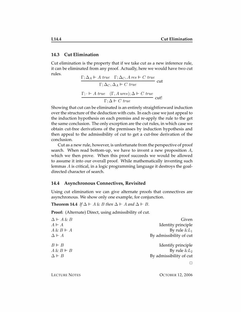
L14.4 Cut Elimination
14.3 Cut Elimination
Cut elimination is the property that if we take cut as a new inference rule,it can be eliminated from any proof. Actually, here we would have two cutrules.
Γ;∆A ` A true Γ;∆C , A res ` C true
Γ;∆C ,∆A ` C truecut
Γ; · ` A true (Γ, A ures);∆ ` C true
Γ;∆ ` C truecut!
Showing that cut can be eliminated is an entirely straightforward inductionover the structure of the deduction with cuts. In each case we just appeal tothe induction hypothesis on each premiss and re-apply the rule to the getthe same conclusion. The only exception are the cut rules, in which case weobtain cut-free derivations of the premisses by induction hypothesis andthen appeal to the admissibility of cut to get a cut-free derivation of theconclusion.
Cut as a new rule, however, is unfortunate from the perspective of proofsearch. When read bottom-up, we have to invent a new proposition A,which we then prove. When this proof succeeds we would be allowedto assume it into our overall proof. While mathematically inventing suchlemmas A is critical, in a logic programming language it destroys the goal-directed character of search.
14.4 Asynchronous Connectives, Revisited
Using cut elimination we can give alternate proofs that connectives areasynchronous. We show only one example, for conjunction.
Theorem 14.4 If ∆ ` A & B then ∆ ` A and ∆ ` B.
Proof: (Alternate) Direct, using admissibility of cut.
∆ ` A & B GivenA ` A Identity principleA & B ` A By rule &L1
∆ ` A By admissibility of cut
B ` B Identify principleA & B ` B By rule &L2
∆ ` B By admissibility of cut
2
LECTURE NOTES OCTOBER 12, 2006
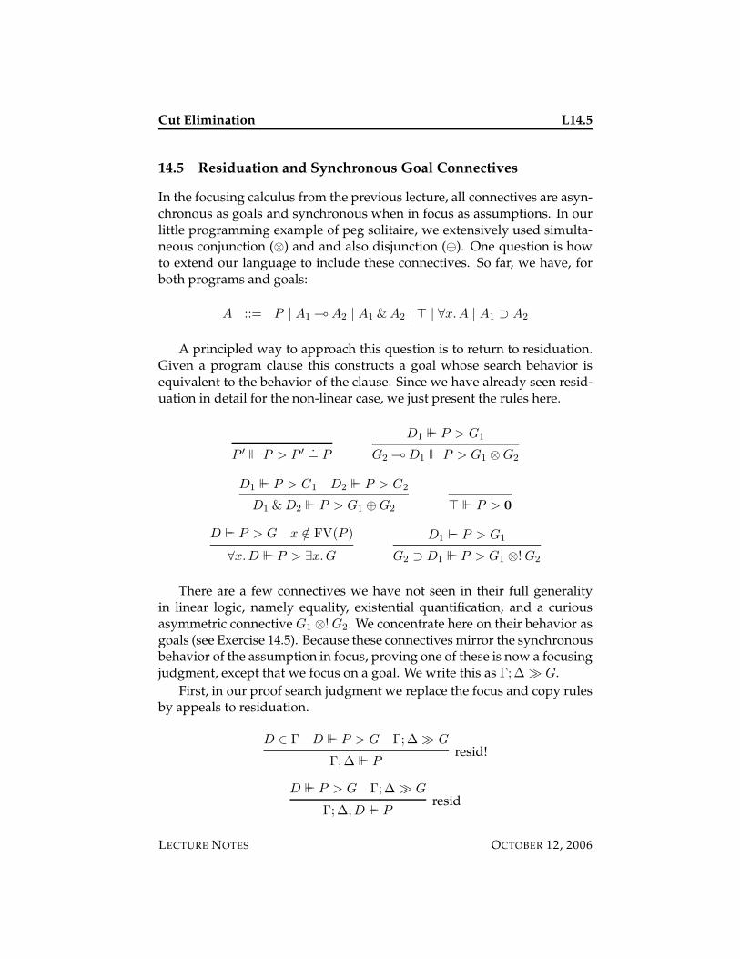
Cut Elimination L14.5
14.5 Residuation and Synchronous Goal Connectives
In the focusing calculus from the previous lecture, all connectives are asyn-chronous as goals and synchronous when in focus as assumptions. In ourlittle programming example of peg solitaire, we extensively used simulta-neous conjunction (⊗) and and also disjunction (⊕). One question is howto extend our language to include these connectives. So far, we have, forboth programs and goals:
A ::= P | A1 ( A2 | A1 & A2 | > | ∀x.A | A1 ⊃ A2
A principled way to approach this question is to return to residuation.Given a program clause this constructs a goal whose search behavior isequivalent to the behavior of the clause. Since we have already seen resid-uation in detail for the non-linear case, we just present the rules here.
P ′ ` P > P ′.= P
D1 ` P > G1
G2 ( D1 ` P > G1 ⊗ G2
D1 ` P > G1 D2 ` P > G2
D1 & D2 ` P > G1 ⊕ G2 > ` P > 0
D ` P > G x /∈ FV(P )
∀x.D ` P > ∃x.G
D1 ` P > G1
G2 ⊃ D1 ` P > G1 ⊗! G2
There are a few connectives we have not seen in their full generalityin linear logic, namely equality, existential quantification, and a curiousasymmetric connective G1 ⊗! G2. We concentrate here on their behavior asgoals (see Exercise 14.5). Because these connectives mirror the synchronousbehavior of the assumption in focus, proving one of these is now a focusingjudgment, except that we focus on a goal. We write this as Γ;∆ � G.
First, in our proof search judgment we replace the focus and copy rulesby appeals to residuation.
D ∈ Γ D ` P > G Γ;∆ � G
Γ;∆ ` Presid!
D ` P > G Γ;∆ � G
Γ;∆,D ` Presid
LECTURE NOTES OCTOBER 12, 2006
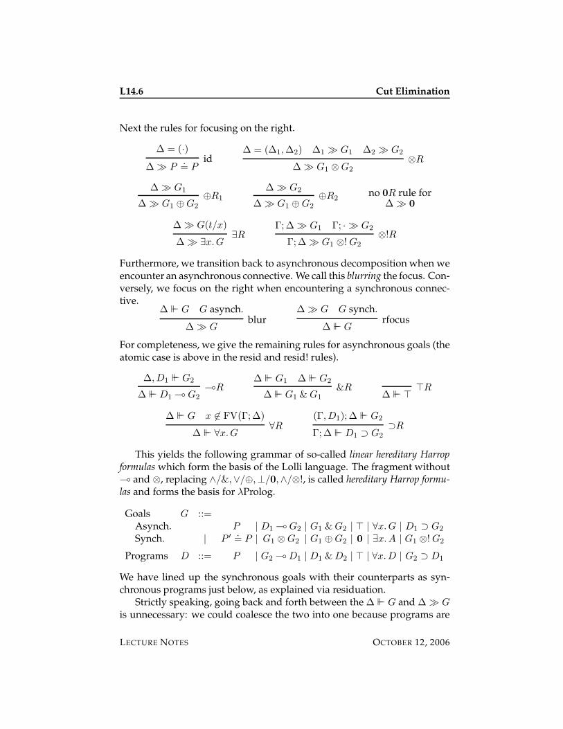
L14.6 Cut Elimination
Next the rules for focusing on the right.
∆ = (·)
∆ � P.= P
id∆ = (∆1,∆2) ∆1 � G1 ∆2 � G2
∆ � G1 ⊗ G2
⊗R
∆ � G1
∆ � G1 ⊕ G2
⊕R1
∆ � G2
∆ � G1 ⊕ G2
⊕R2no 0R rule for
∆ � 0
∆ � G(t/x)
∆ � ∃x.G∃R
Γ;∆ � G1 Γ; · � G2
Γ;∆ � G1 ⊗! G2
⊗!R
Furthermore, we transition back to asynchronous decomposition when weencounter an asynchronous connective. We call this blurring the focus. Con-versely, we focus on the right when encountering a synchronous connec-tive.
∆ ` G G asynch.
∆ � Gblur
∆ � G G synch.
∆ ` Grfocus
For completeness, we give the remaining rules for asynchronous goals (theatomic case is above in the resid and resid! rules).
∆,D1 ` G2
∆ ` D1 ( G2
(R∆ ` G1 ∆ ` G2
∆ ` G1 & G1
&R∆ ` >
>R
∆ ` G x 6∈ FV(Γ;∆)
∆ ` ∀x.G∀R
(Γ,D1);∆ ` G2
Γ;∆ ` D1 ⊃ G2
⊃R
This yields the following grammar of so-called linear hereditary Harropformulas which form the basis of the Lolli language. The fragment without( and ⊗, replacing ∧/&,∨/⊕,⊥/0,∧/⊗!, is called hereditary Harrop formu-las and forms the basis for λProlog.
Goals G ::=Asynch. P | D1 ( G2 | G1 & G2 | > | ∀x.G | D1 ⊃ G2
Synch. | P ′ .= P | G1 ⊗ G2 | G1 ⊕ G2 | 0 | ∃x.A | G1 ⊗! G2
Programs D ::= P | G2 ( D1 | D1 & D2 | > | ∀x.D | G2 ⊃ D1
We have lined up the synchronous goals with their counterparts as syn-chronous programs just below, as explained via residuation.
Strictly speaking, going back and forth between the ∆ ` G and ∆ � G
is unnecessary: we could coalesce the two into one because programs are
LECTURE NOTES OCTOBER 12, 2006
Cut Elimination L14.7
always fully synchronous. However, it highlights the difference betweenthe synchronous and asynchronous right rules: Asynchronous decomposi-tion in ∆ ` G is automatic and involves no choice, synchronous decom-position ∆ � G involves a significant choice and may fail. Moreover, injust about any logical extension of focusing beyond this fragment, we needto pause when the goal becomes synchronous during the asynchronousdecomposition phase and consider whether to focus on an assumption in-stead. Here, this would always fail.
In practice, it is convenient to admit an even slightly richer set of goals,whose meaning can be explained either via a transformation to the connec-tives already shown above or directly via synchronous or asynchronousrules for them (see Exercise 14.3).
14.6 Completeness of Focusing
Soundness of the focusing system is easy to see, since each rule is a restric-tion of the corresponding left and right rules for the non-focused sequentcalculus. Completeness is somewhat more difficult. We can continue thepath mapped out in the proof that various connectives are asynchronousas goals, proving that the same connectives are indeed synchronous as pro-grams. Alternatively, we can prove a generalization of the cut elimina-tion results for focused derivations and use that in an overall completenessproof. The references below give some pointers to the two different stylesof proof in the literature.
14.7 Historical Notes
Cut elimination, one of the most fundamental theorems in logic, is due toGentzen [3], who introduced the sequent calculus and natural deductionfor both classical and intuitionistic logic and showed cut elimination. Hisformulation of the sequent calculus had explicit rules for exchange, weak-ing, and contraction, which make the proof somewhat more tedious thanthe one we presented here. I first provided proofs by simple nested struc-tural induction, formalized in a logical framework, for intuitionistic andclassical [5, 6] as well as linear logic [4].
Andreoli introduced focusing for classical linear logic [1] and proved itscompleteness through a number of inversion and admissibility properties.An alternative proof using cut elimination as a central lemma, applied tointuitionistic linear logic was given by Chaudhuri [2].
LECTURE NOTES OCTOBER 12, 2006
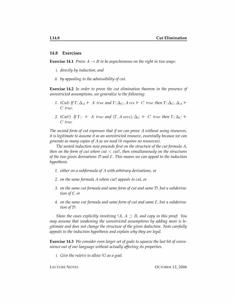
L14.8 Cut Elimination
14.8 Exercises
Exercise 14.1 Prove A ( B to be asynchronous on the right in two ways:
i. directly by induction, and
ii. by appealing to the admissibility of cut.
Exercise 14.2 In order to prove the cut elimination theorem in the presence ofunrestricted assumptions, we generalize to the following:
1. (Cut) If Γ;∆A ` A true and Γ;∆C , A res ` C true then Γ;∆C ,∆A `
C true .
2. (Cut!) If Γ; · ` A true and (Γ, A ures);∆C ` C true then Γ;∆C `
C true
The second form of cut expresses that if we can prove A without using resources,it is legitimate to assume it as an unrestricted resource, essentially because we cangenerate as many copies of A as we need (it requires no resources).
The nested induction now proceeds first on the structure of the cut formula A,then on the form of cut where cut < cut!, then simultaneously on the structuresof the two given derivations D and E . This means we can appeal to the inductionhypothesis
1. either on a subformula of A with arbitrary derivations, or
2. on the same formula A where cut! appeals to cut, or
3. on the same cut formula and same form of cut and same D, but a subderiva-tion of E , or
4. on the same cut formula and same form of cut and same E , but a subderiva-tion of D.
Show the cases explicitly involving !A, A ⊃ B, and copy in this proof. Youmay assume that weakening the unrestricted assumptions by adding more is le-gitimate and does not change the structure of the given deduction. Note carefullyappeals to the induction hypothesis and explain why they are legal.
Exercise 14.3 We consider even larger set of goals to squeeze the last bit of conve-nience out of our language without actually affecting its properties.
i. Give the rule(s) to allow !G as a goal.
LECTURE NOTES OCTOBER 12, 2006
Cut Elimination L14.9
ii. Give the rule(s) to allow 1 as a goal.
iii. We could allow simultaneous conjunction on the left-hand side of linear im-plication goals, because (D1 ⊗D2) ( G is equivalent to D1 ( (D2 ( G),which lies within the permitted fragment. Explore which formulas R couldbe allowed in goals of the form R ( G because they can be eliminated by alocal equivalence-preserving transformation such as the one for ⊗.
iv. Now explore which formulas S could be allowed in goals of the form S ⊃ G
without affecting the essence of the language.
Exercise 14.4 Prove that the focusing system with left and right rules is equiva-lent to the system with only right rules and residuation for atomic goals.
Exercise 14.5 Through residuation, we have introduced two new connectives tolinear logic, A ⊗! B and P ′ .
= P , but we have only considered their right rules.Give corresponding left rules for them in the sequent calculus and prove cut
elimination and identity for your rules.
14.9 References
[1] Jean-Marc Andreoli. Logic programming with focusing proofs in linearlogic. Journal of Logic and Computation, 2(3):297–347, 1992.
[2] Kaustuv Chaudhuri. The Focused Inverse Method for Linear Logic. PhDthesis, Carnegie Mellon University, 2006. To appear.
[3] Gerhard Gentzen. Untersuchungen uber das logische Schließen. Math-ematische Zeitschrift, 39:176–210, 405–431, 1935. English translation inM. E. Szabo, editor, The Collected Papers of Gerhard Gentzen, pages 68–131, North-Holland, 1969.
[4] Frank Pfenning. Structural cut elimination in linear logic. Technical Re-port CMU-CS-94-222, Department of Computer Science, Carnegie Mel-lon University, December 1994.
[5] Frank Pfenning. A structural proof of cut elimination and its represen-tation in a logical framework. Technical Report CMU-CS-94-218, De-partment of Computer Science, Carnegie Mellon University, November1994.
[6] Frank Pfenning. Structural cut elimination I. intuitionistic and classicallogic. Information and Computation, 157(1/2):84–141, March 2000.
LECTURE NOTES OCTOBER 12, 2006

L14.10 Cut Elimination
LECTURE NOTES OCTOBER 12, 2006
15-819K: Logic Programming
Lecture 15
Resource Management
Frank Pfenning
October 17, 2006
In this lecture we address the resource management problem in linear logicprogramming. We also give some small but instructive examples of linearlogic programming, supplementing the earlier peg solitaire code.
15.1 Input/Output Interpretation of Resources
Reconsider the rule for simultaneous conjunction as a goal.
∆ = (∆1,∆2) ∆1 ` G1 ∆2 ` G2
∆ ` G1 ⊗ G2
⊗R
The difficulty in using this rule in proof search is that, as written, we haveto “guess” the right way to split the resources ∆ into two. Clearly, enumer-ating all possible ways to split ∆ will be very inefficient, and also difficultfor the programmer to predict.
Instead, we pass all resources to the goal G1 and then pass the ones thatwere not consumed in the derivation of G1 to G2. We write
∆I \ ∆O ` G
where ∆I is the input context and ∆O is the output context generated bythe proof search for G. The invariant we preserve is that
∆I \ ∆O ` G iff ∆I − ∆O ` G
where ∆I − ∆O subtracts the resources in ∆O from the resources in ∆I .It is convenient to keep ∆I and ∆O ordered, so that this difference can becomputed component by component (see below).
LECTURE NOTES OCTOBER 17, 2006
L15.2 Resource Management
Now the rule for simultaneous conjunction is
∆I \ ∆M ` G1 ∆M \ ∆O ` G2
∆I \ ∆O ` G1 ⊗ G2
⊗R.
It is easy to verify that the above invariant holds for this rule. More for-mally, this would be part of a soundness and completeness proof for theinput/output interpretation of resources.
15.2 Slack Resources
The simple input/output interpretation for resources breaks down for con-sumptive truth (>). Recall the rule
∆ ` >>R
which translates to∆I ⊇ ∆O
∆I \ ∆O ` >>R
because > may consume any of its input but does not need to. Now we areback at the original problem, since we certainly do not want to enumerateall possible subsets of ∆I blindly.
Instead, we pass on all the input resources, but also a flag to indicatethat all of these resources could have been consumed. That means if theyare left over at the end, we can succeed instead of having to fail. We writethe judgment as
∆I \ ∆O ` v G
where v = 0 means G used exactly the resources in ∆I − ∆O, while v = 1means G could also have consumed additional resources from ∆O. Nowour invariants are:
i. ∆I \ ∆O ` 0 G iff ∆I − ∆O ` G
ii. ∆I \ ∆O ` 1 G iff ∆I − ∆O,∆′ ` G for any ∆O ⊇ ∆′.
The right rule for > with slack is just
∆I \ ∆I ` 1 >>R.
LECTURE NOTES OCTOBER 17, 2006
Resource Management L15.3
In contrast, the rule for equality which requires the linear context to beempty is
∆I \ ∆I ` 0 t.= t
.=R.
As far as resources are concerned, the only difference is whether slack isallowed (v = 1) or not (v = 0).
We now briefly return to simultaneous conjunction. There is slack inthe deduction for G1 ⊗ G2 if there is slack on either side: any remainingresources could be pushed up into either of the two subderivations as longas there is slack in at least one.
∆I \ ∆M ` v G1 ∆M \ ∆O `w G2
∆I \ ∆O ` v∨w G1 ⊗ G2
⊗R.
Here v ∨ w is the usual Boolean disjunction between the two flags: it is 0 ifboth disjuncts are 0 and 1 otherwise.
15.3 Strict Resources
Unfortunately, there is still an issue in that resource management does nottake into account all information it should. There are examples in the litera-ture [2], but they are not particularly natural. For an informal explanation,consider the overall query ∆ ` G. We run this as ∆ \ ∆O ` v G, where∆O and v are returned. We then have to check that all input has indeed beconsumed by verifying that ∆O is empty. If ∆O is not empty, we have tofail this attempt and backtrack.
We would like to achieve that we fail as soon as possible when no proofcan exist due to resource management issues. In the present system wemay sometimes run to completion only to note at that point that we failedto consume all resources. We can avoid this issue by introducing yet onemore distinction into our resource management judgment by separatingout strict resources. Unlike ∆I , which represents resources which may beused, Ξ represent resources which must be used in a proof.
Ξ;∆I \ ∆O ` v G
The invariant does not get significantly more complicated.
i. Ξ;∆I \ ∆O ` 0 G iff Ξ,∆I − ∆O ` G
ii. Ξ;∆I \ ∆O ` 1 G iff Ξ,∆I − ∆O,∆′ ` G for all ∆O ⊇ ∆′.
LECTURE NOTES OCTOBER 17, 2006
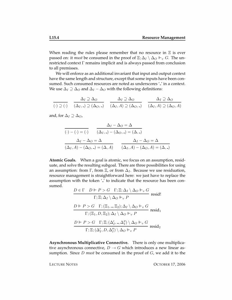
L15.4 Resource Management
When reading the rules please remember that no resource in Ξ is everpassed on: it must be consumed in the proof of Ξ;∆I \ ∆O ` v G. The un-restricted context Γ remains implicit and is always passed from conclusionto all premisses.
We will enforce as an additional invariant that input and output contexthave the same length and structure, except that some inputs have been con-sumed. Such consumed resources are noted as underscores ‘ ’ in a context.We use ∆I ⊇ ∆O and ∆I − ∆O with the following definitions:
(·) ⊇ (·)
∆I ⊇ ∆O
(∆I , ) ⊇ (∆O, )
∆I ⊇ ∆O
(∆I , A) ⊇ (∆O, )
∆I ⊇ ∆O
(∆I , A) ⊇ (∆O, A)
and, for ∆I ⊇ ∆O,
(·) − (·) = (·)
∆I − ∆O = ∆
(∆I , ) − (∆O, ) = (∆, )
∆I − ∆O = ∆
(∆I , A) − (∆O, ) = (∆, A)
∆I − ∆O = ∆
(∆I , A) − (∆O, A) = (∆, )
Atomic Goals. When a goal is atomic, we focus on an assumption, resid-uate, and solve the resulting subgoal. There are three possibilities for usingan assumption: from Γ, from Ξ, or from ∆I . Because we use residuation,resource management is straightforward here: we just have to replace theassumption with the token ‘ ’ to indicate that the resource has been con-sumed.
D ∈ Γ D ` P > G Γ;Ξ;∆I \ ∆O ` v G
Γ;Ξ;∆I \ ∆O ` v Presid!
D ` P > G Γ; (Ξ1, ,Ξ2);∆I \ ∆O ` v G
Γ; (Ξ1,D,Ξ2);∆I \ ∆O ` v Presid1
D ` P > G Γ;Ξ; (∆′
I, ,∆′′
I) \ ∆O ` v G
Γ;Ξ; (∆′
I,D,∆′′
I) \ ∆O ` v P
resid2
Asynchronous Multiplicative Connective. There is only one multiplica-tive asynchronous connective, D ( G which introduces a new linear as-sumption. Since D must be consumed in the proof of G, we add it to the
LECTURE NOTES OCTOBER 17, 2006
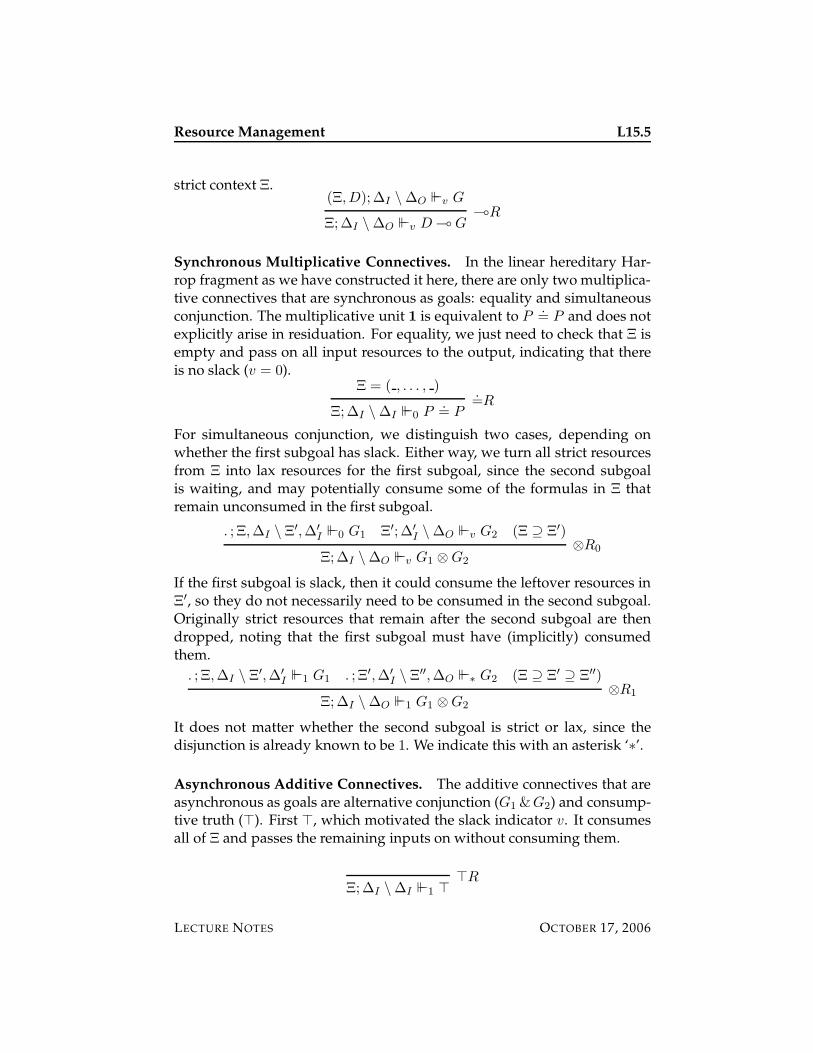
Resource Management L15.5
strict context Ξ.(Ξ,D);∆I \ ∆O ` v G
Ξ;∆I \ ∆O ` v D ( G(R
Synchronous Multiplicative Connectives. In the linear hereditary Har-rop fragment as we have constructed it here, there are only two multiplica-tive connectives that are synchronous as goals: equality and simultaneousconjunction. The multiplicative unit 1 is equivalent to P
.= P and does not
explicitly arise in residuation. For equality, we just need to check that Ξ isempty and pass on all input resources to the output, indicating that thereis no slack (v = 0).
Ξ = ( , . . . , )
Ξ;∆I \ ∆I ` 0 P.= P
.=R
For simultaneous conjunction, we distinguish two cases, depending onwhether the first subgoal has slack. Either way, we turn all strict resourcesfrom Ξ into lax resources for the first subgoal, since the second subgoalis waiting, and may potentially consume some of the formulas in Ξ thatremain unconsumed in the first subgoal.
. ; Ξ,∆I \ Ξ′,∆′
I` 0 G1 Ξ′;∆′
I\ ∆O ` v G2 (Ξ ⊇ Ξ′)
Ξ;∆I \ ∆O ` v G1 ⊗ G2
⊗R0
If the first subgoal is slack, then it could consume the leftover resources inΞ′, so they do not necessarily need to be consumed in the second subgoal.Originally strict resources that remain after the second subgoal are thendropped, noting that the first subgoal must have (implicitly) consumedthem.
. ; Ξ,∆I \ Ξ′,∆′
I` 1 G1 . ; Ξ′,∆′
I\ Ξ′′,∆O ` ∗ G2 (Ξ ⊇ Ξ′ ⊇ Ξ′′)
Ξ;∆I \ ∆O ` 1 G1 ⊗ G2
⊗R1
It does not matter whether the second subgoal is strict or lax, since thedisjunction is already known to be 1. We indicate this with an asterisk ‘∗’.
Asynchronous Additive Connectives. The additive connectives that areasynchronous as goals are alternative conjunction (G1 & G2) and consump-tive truth (>). First >, which motivated the slack indicator v. It consumesall of Ξ and passes the remaining inputs on without consuming them.
Ξ;∆I \ ∆I ` 1 >>R
LECTURE NOTES OCTOBER 17, 2006
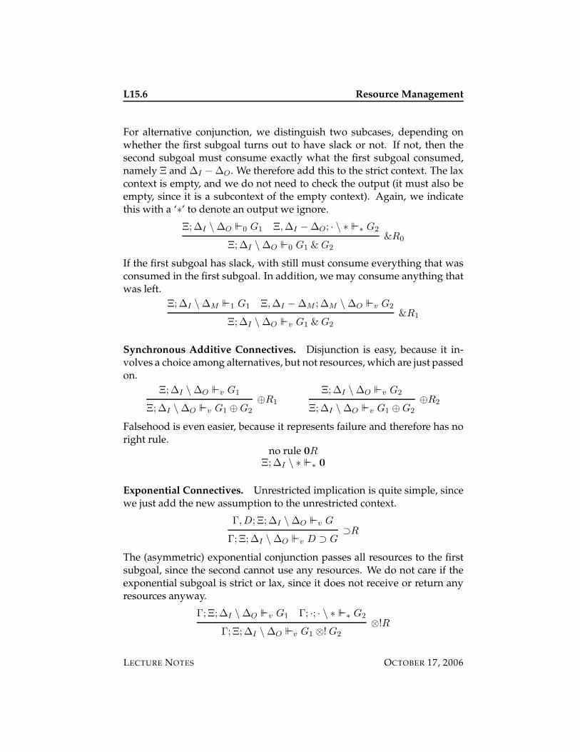
L15.6 Resource Management
For alternative conjunction, we distinguish two subcases, depending onwhether the first subgoal turns out to have slack or not. If not, then thesecond subgoal must consume exactly what the first subgoal consumed,namely Ξ and ∆I − ∆O. We therefore add this to the strict context. The laxcontext is empty, and we do not need to check the output (it must also beempty, since it is a subcontext of the empty context). Again, we indicatethis with a ‘∗’ to denote an output we ignore.
Ξ;∆I \ ∆O ` 0 G1 Ξ,∆I − ∆O; · \ ∗ ` ∗ G2
Ξ;∆I \ ∆O ` 0 G1 & G2
&R0
If the first subgoal has slack, with still must consume everything that wasconsumed in the first subgoal. In addition, we may consume anything thatwas left.
Ξ;∆I \ ∆M ` 1 G1 Ξ,∆I − ∆M ;∆M \ ∆O ` v G2
Ξ;∆I \ ∆O ` v G1 & G2
&R1
Synchronous Additive Connectives. Disjunction is easy, because it in-volves a choice among alternatives, but not resources, which are just passedon.
Ξ;∆I \ ∆O ` v G1
Ξ;∆I \ ∆O ` v G1 ⊕ G2
⊕R1
Ξ;∆I \ ∆O ` v G2
Ξ;∆I \ ∆O ` v G1 ⊕ G2
⊕R2
Falsehood is even easier, because it represents failure and therefore has noright rule.
no rule 0RΞ;∆I \ ∗ ` ∗ 0
Exponential Connectives. Unrestricted implication is quite simple, sincewe just add the new assumption to the unrestricted context.
Γ,D; Ξ;∆I \ ∆O ` v G
Γ;Ξ;∆I \ ∆O ` v D ⊃ G⊃R
The (asymmetric) exponential conjunction passes all resources to the firstsubgoal, since the second cannot use any resources. We do not care if theexponential subgoal is strict or lax, since it does not receive or return anyresources anyway.
Γ;Ξ;∆I \ ∆O ` v G1 Γ; ·; · \ ∗ ` ∗ G2
Γ;Ξ;∆I \ ∆O ` v G1 ⊗! G2
⊗!R
LECTURE NOTES OCTOBER 17, 2006
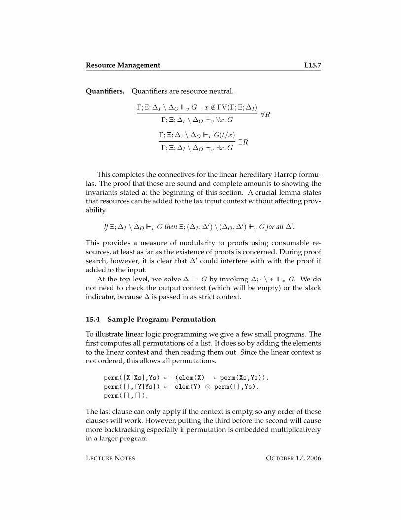
Resource Management L15.7
Quantifiers. Quantifiers are resource neutral.
Γ;Ξ;∆I \ ∆O ` v G x /∈ FV(Γ;Ξ;∆I)
Γ; Ξ;∆I \ ∆O ` v ∀x.G∀R
Γ;Ξ;∆I \ ∆O ` v G(t/x)
Γ; Ξ;∆I \ ∆O ` v ∃x.G∃R
This completes the connectives for the linear hereditary Harrop formu-las. The proof that these are sound and complete amounts to showing theinvariants stated at the beginning of this section. A crucial lemma statesthat resources can be added to the lax input context without affecting prov-ability.
If Ξ;∆I \ ∆O ` v G then Ξ; (∆I ,∆′) \ (∆O,∆′) ` v G for all ∆′.
This provides a measure of modularity to proofs using consumable re-sources, at least as far as the existence of proofs is concerned. During proofsearch, however, it is clear that ∆′ could interfere with with the proof ifadded to the input.
At the top level, we solve ∆ ` G by invoking ∆; · \ ∗ ` ∗ G. We donot need to check the output context (which will be empty) or the slackindicator, because ∆ is passed in as strict context.
15.4 Sample Program: Permutation
To illustrate linear logic programming we give a few small programs. Thefirst computes all permutations of a list. It does so by adding the elementsto the linear context and then reading them out. Since the linear context isnot ordered, this allows all permutations.
perm([X|Xs],Ys) ◦− (elem(X) ( perm(Xs,Ys)).
perm([],[Y|Ys]) ◦− elem(Y) ⊗ perm([],Ys).
perm([],[]).
The last clause can only apply if the context is empty, so any order of theseclauses will work. However, putting the third before the second will causemore backtracking especially if permutation is embedded multiplicativelyin a larger program.
LECTURE NOTES OCTOBER 17, 2006
L15.8 Resource Management
15.5 Sample Program: Depth-First Search
Imperative algorithms for depth-first search mark nodes that have beenvisited to prevent looping. We can model this in a linear logic program bystarting with a linear assumption node(x) for every node x and consumingthis assumption when visiting a node. This means that a node cannot beused more than once, preventing looping.
We assume a predicate edge(x,y) which holds whenever there is a di-rected edge from x to y.
dfs(X,Y) ◦− edge(X,Y).
dfs(X,Y) ◦− edge(X,Z) ⊗ node(Z) ⊗ dfs(Z,Y).
This by itself is note quite enough because not all nodes might be visited.We can allow this with the following top-level call
path(X,Y) ◦− node(X) ⊗ dfs(X,Y) ⊗ >.
15.6 Sample Program: Stateful Queues
In Lecture 11 we have seen how to implement a queue with a differencelist, but we had to pass the queue around as an argument to any predicatewanting to use it. We can also maintain the queue in the linear context.Recall that we used a list of instructions enq(x) and deq(x), and that at theend the queue must be empty.
queue(Is) ◦− (front(B) ⊗ back(B) ( q(Is)).
q([enq(X)|Is]) ◦− back([X|B]) ⊗ (back(B) ( q(Is)).
q([deq(X)|Is]) ◦− front([X|Xs]) ⊗ (front(Xs) ( q(Is)).
q([]) ◦− front([]) ⊗ back([]).
In this version, the dequeuing may borrow against future enqueue opera-tions (see Exercise 15.2).
It is tempting to think we might use the linear context itself as a kindof queue, similar to the permutation program, but using cut ‘!’ to avoidgetting all solution. This actually does not work, since the linear context ismaintained as a stack: most recently made assumptions are tried first.
LECTURE NOTES OCTOBER 17, 2006
Resource Management L15.9
15.7 Historical Notes
Resource management for linear logic programming was first consideredby Hodas and Miller in the design of Lolli [7, 8]. The original designunderestimated the importance of consumptive truth, which was later re-paired by adding the slack indicator [5] and then the strict context [1, 2].Primitive operations on the contexts are still quite expensive, which wasaddressed subsequently through so-called tag frames which implement thecontext management system presented here in an efficient way [6, 9].
An alternative approach to resource management is to use Boolean con-straints to connect resources in different branches of the proof tree, devel-oped by Harland and Pym [3, 4]. This is more general, because one is notcommitted to depth-first search, but also potentially more expensive.
An implementation of the linear logic programming language Lolli inStandard ML can be found at http://www.cs.cmu.edu/~fp/lolli. Thecode presented in this course, additional puzzles, a propositional theoremprover, and more example can be found in the distribution.
15.8 Exercises
Exercise 15.1 Prove carefully that the perm predicate does implement permuta-tion when invoked in the empty context. You will need to generalize this statementto account for intermediate states in the computation.
Exercise 15.2 Modify the stateful queue program so it fails if an element is de-queued before it is enqueued.
Exercise 15.3 Give an implementation of a double-ended queue in linear logicprogramming, where elements can be both enqueued and dequeued at both ends.
Exercise 15.4 Sometimes, linear logic appears excessively pedantic in that all re-source must be used. In affine logic resources may be used at most once. De-velop the connectives of affine logic, its asynchronous fragment, residuation, andresource management for affine logic. Discuss the simplifications in comparisonwith linear logic (if any).
Exercise 15.5 Philosophers have developed relevance logic in order to capturethat in a proof of A implies B, some use of A should be made in the proof of B.Strict logic is a variant of relevance logic where we think of strict assumptions asresources which must be used at least once in a proof. Develop the connectives ofstrict logic, its asynchronous fragment, residuation, and resource management forstrict logic. Discuss the simplifications in comparison with linear logic (if any).
LECTURE NOTES OCTOBER 17, 2006
L15.10 Resource Management
Exercise 15.6 In the resource managment system we employed a relatively high-level logical system, without goal stack, failure continuation, or explicit unifica-tion. Extend the abstract machine which uses these mechanisms by adding resourcemanagement as given in this lecture.
Because we can make linear or unrestricted assumptions in the course of search,not all information associated with a predicate symbol p is static, in the globalprogram. This means the rule for atomic goals must change. You should fix theorder in which assumptions are tried by using most recently made assumptionsfirst and fall back on the static program when all dynamic possibilities have beenexhausted.
15.9 References
[1] Iliano Cervesato, Joshua S. Hodas, and Frank Pfenning. Efficient re-source management for linear logic proof search. In R. Dyckhoff,H. Herre, and P. Schroeder-Heister, editors, Proceedings of the 5th In-ternational Workshop on Extensions of Logic Programming, pages 67–81,Leipzig, Germany, March 1996. Springer-Verlag LNAI 1050.
[2] Iliano Cervesato, Joshua S. Hodas, and Frank Pfenning. Efficient re-source management for linear logic proof search. Theoretical ComputerScience, 232(1–2):133–163, February 2000. Special issue on Proof Searchin Type-Theoretic Languages, D. Galmiche and D. Pym, editors.
[3] James Harland and David J. Pym. Resource distribution via Booleanconstraints. In W. McCune, editor, Proceedings of the 14th Interna-tional Conference on Automated Deduction (CADE-14), pages 222–236,Townsville, Australia, July 1997. Springer Verlag LNCS 1249.
[4] James Harland and David J. Pym. Resource distribution via Booleanconstraints. ACM Transactions on Computational Logic, 4(1):56–90, 2003.
[5] Joshua S. Hodas. Logic Programming in Intuitionistic Linear Logic: Theory,Design, and Implementation. PhD thesis, University of Pennsylvania, De-partment of Computer and Information Science, 1994.
[6] Joshua S. Hodas, Pablo Lopez, Jeffrey Polakow, Lubomira Stoilova,and Ernesto Pimentel. A tag-frame system of resource managementfor proof search in linear-logic programming. In J. Bradfield, edi-tor, Proceedings of the 16th International Workshop on Computer ScienceLogic (CSL’02), pages 167–182, Edinburgh, Scotland, September 2002.Springer Verlag LNCS 2471.
LECTURE NOTES OCTOBER 17, 2006
Resource Management L15.11
[7] Joshua S. Hodas and Dale Miller. Logic programming in a fragmentof intuitionistic linear logic. In Proceedings of the 6th Annual Symposiumon Logic in Computer Science (LICS’91), pages 32–42, Amsterdam, TheNetherlands, July 1991. IEEE Computer Society Press.
[8] Joshua S. Hodas and Dale Miller. Logic programming in a fragment ofintuitionistic linear logic. Information and Computation, 110(2):327–365,1994.
[9] Pablo Lopez and Jeffrey Polakow. Implementing efficient resourcemanagement for linear logic programming. In Franz Baader and An-drei Voronkov, editors, Proceedings of the 11th International Conferenceon Logic for Programming, Artificial Intelligence, and Reasoning (LPAR’04),pages 528–543, Montevideo, Uruguay, March 2005. Springer VerlagLNCS 3452.
LECTURE NOTES OCTOBER 17, 2006

L15.12 Resource Management
LECTURE NOTES OCTOBER 17, 2006
15-819K: Logic Programming
Lecture 16
Substitution Semantics
Frank Pfenning
October 24, 2006
In this lecture we introduce a semantics with an explicit substitution, inpreparation for presenting various program analyses later. The semanticswill have the property that its goals appear exactly as in the original pro-grams, with a separate substitution as part of the judgment. We also re-viewed potential project areas during lecture, which is not represented inthese notes.
16.1 Semantic Levels
When designing a program analysis we need to consider which level of se-mantic description is appropriate. This is relevant both for designing andproving the correctness of the analysis, which could be either simple ordifficult, depending on our starting point. By the “level of semantic de-scription” we mean here the spectrum from the logical semantics (in whichwe can only talk about truth), through one where subgoal order is explicit,to one with a failure continuation. An additional dimension is if a substi-tution is explicit in the semantics.
Which kind of semantics is appropriate, for example, for defining modeanalysis? We would like to stay as high-level as possible, while still beingable to express the property in question. Because mode analysis dependson subgoal order, one would expect to make subgoal order explicit. More-over, since groundedness is a property of the substitution that is applied,we also should make a substitution explicit during computation. On theother hand, modes do not interact with backtracking, so we do not expectto need a failure continuation.
We take here a slight shortcut, using a semantics with an explicit sub-stitution, but not a subgoal stack. Of course, it is possible to give such a
LECTURE NOTES OCTOBER 24, 2006
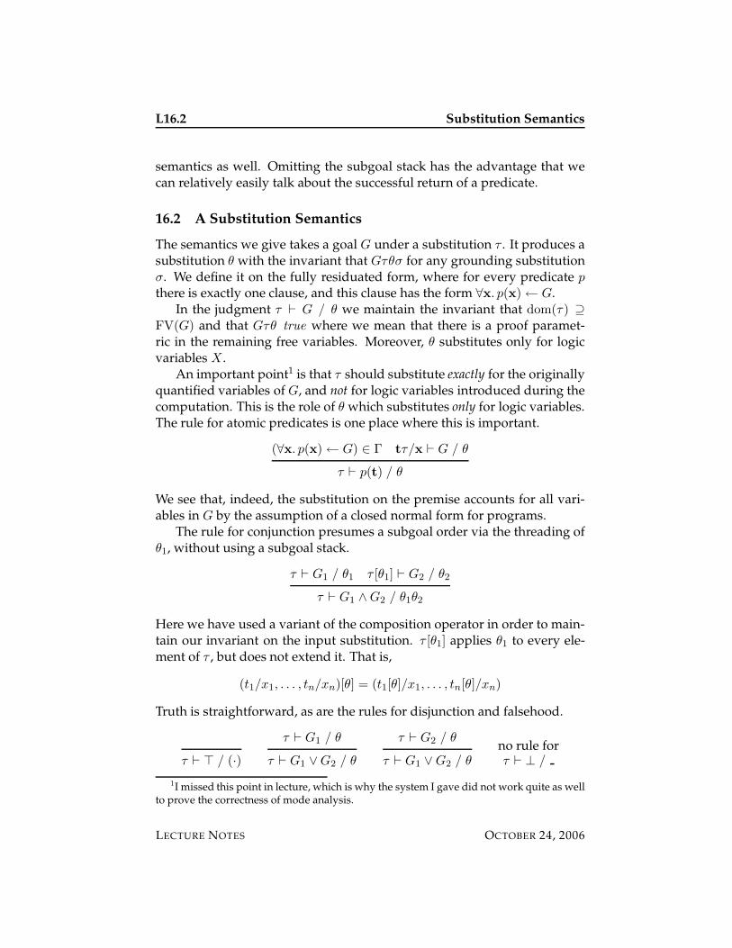
L16.2 Substitution Semantics
semantics as well. Omitting the subgoal stack has the advantage that wecan relatively easily talk about the successful return of a predicate.
16.2 A Substitution Semantics
The semantics we give takes a goal G under a substitution τ . It produces asubstitution θ with the invariant that Gτθσ for any grounding substitutionσ. We define it on the fully residuated form, where for every predicate p
there is exactly one clause, and this clause has the form ∀x. p(x)← G.In the judgment τ ` G / θ we maintain the invariant that dom(τ) ⊇
FV(G) and that Gτθ true where we mean that there is a proof paramet-ric in the remaining free variables. Moreover, θ substitutes only for logicvariables X.
An important point1 is that τ should substitute exactly for the originallyquantified variables of G, and not for logic variables introduced during thecomputation. This is the role of θ which substitutes only for logic variables.The rule for atomic predicates is one place where this is important.
(∀x. p(x)← G) ∈ Γ tτ/x ` G / θ
τ ` p(t) / θ
We see that, indeed, the substitution on the premise accounts for all vari-ables in G by the assumption of a closed normal form for programs.
The rule for conjunction presumes a subgoal order via the threading ofθ1, without using a subgoal stack.
τ ` G1 / θ1 τ [θ1] ` G2 / θ2
τ ` G1 ∧G2 / θ1θ2
Here we have used a variant of the composition operator in order to main-tain our invariant on the input substitution. τ [θ1] applies θ1 to every ele-ment of τ , but does not extend it. That is,
(t1/x1, . . . , tn/xn)[θ] = (t1[θ]/x1, . . . , tn[θ]/xn)
Truth is straightforward, as are the rules for disjunction and falsehood.
τ ` > / (·)
τ ` G1 / θ
τ ` G1 ∨G2 / θ
τ ` G2 / θ
τ ` G1 ∨G2 / θno rule forτ ` ⊥ /
1I missed this point in lecture, which is why the system I gave did not work quite as wellto prove the correctness of mode analysis.
LECTURE NOTES OCTOBER 24, 2006
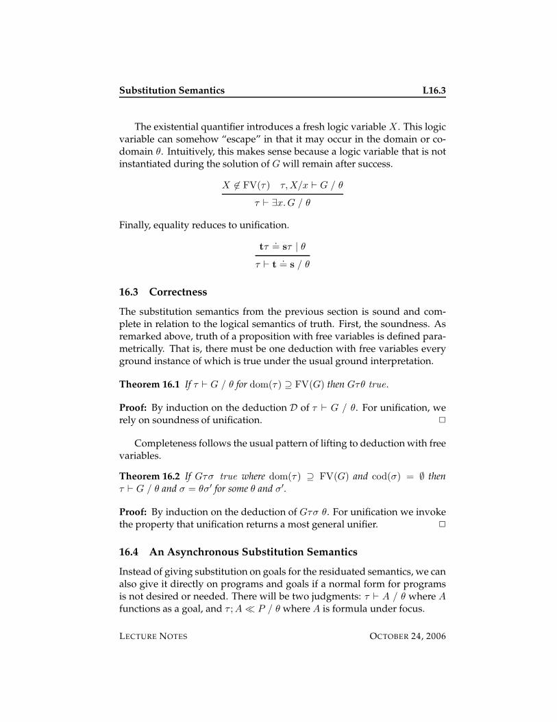
Substitution Semantics L16.3
The existential quantifier introduces a fresh logic variable X. This logicvariable can somehow “escape” in that it may occur in the domain or co-domain θ. Intuitively, this makes sense because a logic variable that is notinstantiated during the solution of G will remain after success.
X 6∈ FV(τ) τ,X/x ` G / θ
τ ` ∃x.G / θ
Finally, equality reduces to unification.
tτ.= sτ | θ
τ ` t.= s / θ
16.3 Correctness
The substitution semantics from the previous section is sound and com-plete in relation to the logical semantics of truth. First, the soundness. Asremarked above, truth of a proposition with free variables is defined para-metrically. That is, there must be one deduction with free variables everyground instance of which is true under the usual ground interpretation.
Theorem 16.1 If τ ` G / θ for dom(τ) ⊇ FV(G) then Gτθ true .
Proof: By induction on the deduction D of τ ` G / θ. For unification, werely on soundness of unification. 2
Completeness follows the usual pattern of lifting to deduction with freevariables.
Theorem 16.2 If Gτσ true where dom(τ) ⊇ FV(G) and cod(σ) = ∅ thenτ ` G / θ and σ = θσ′ for some θ and σ′.
Proof: By induction on the deduction of Gτσ θ. For unification we invokethe property that unification returns a most general unifier. 2
16.4 An Asynchronous Substitution Semantics
Instead of giving substitution on goals for the residuated semantics, we canalso give it directly on programs and goals if a normal form for programsis not desired or needed. There will be two judgments: τ ` A / θ where A
functions as a goal, and τ ;A� P / θ where A is formula under focus.
LECTURE NOTES OCTOBER 24, 2006
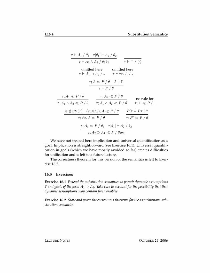
L16.4 Substitution Semantics
τ ` A1 / θ1 τ [θ1] ` A2 / θ2
τ ` A1 ∧A2 / θ1θ2 τ ` > / (·)
omitted hereτ ` A1 ⊃ A2 /
omitted hereτ ` ∀x.A /
τ ;A� P / θ A ∈ Γ
τ ` P / θ
τ ;A1 � P / θ
τ ;A1 ∧A2 � P / θ
τ ;A2 � P / θ
τ ;A1 ∧A2 � P / θno rule for
τ ;> � P /
X /∈ FV(τ) (τ,X/x);A� P / θ
τ ;∀x.A� P / θ
P ′τ.= Pτ | θ
τ ;P ′ � P / θ
τ ;A1 � P / θ1 τ [θ1] ` A2 / θ2
τ ;A2 ⊃ A1 � P / θ1θ2
We have not treated here implication and universal quantification as agoal. Implication is straightforward (see Exercise 16.1). Universal quantifi-cation in goals (which we have mostly avoided so far) creates difficultiesfor unification and is left to a future lecture.
The correctness theorem for this version of the semantics is left to Exer-cise 16.2.
16.5 Exercises
Exercise 16.1 Extend the substitution semantics to permit dynamic assumptionsΓ and goals of the form A1 ⊃ A2. Take care to account for the possibility that thatdynamic assumptions may contain free variables.
Exercise 16.2 State and prove the correctness theorems for the asynchronous sub-stitution semantics.
LECTURE NOTES OCTOBER 24, 2006
15-819K: Logic Programming
Lecture 17
Mode Checking
Frank Pfenning
October 26, 2006
In this lecture we present modes to capture directionality in logic programs.Mode checking helps to catch programming errors and also allows for moreefficient implementation. It is based on a form of abstract interpretationwhere substitutions are approximated by a two-element lattice: completelyunknown terms, and terms known to be ground.
17.1 Modes
We have already informally used modes in the discussion of logic programs.For example, we can execute certain predicates in multiple directions, butthis is impossible in other directions. We use modes + for input, - for outputand * for bi-directional arguments that are not designated as input or output.
We define the meaning as follows:
• Input arguments (+) must be ground when a predicate is invoked. Itis an error if the mode analysis cannot establish this for a call to apredicate.
• Output arguments (-) must be ground when a predicate succeeds. Itis an error if the mode analysis cannot establish this for the definitionof a predicate.
From this we can deduce immediately:
• Input arguments (+) can be assumed to be ground when analyzing thedefinition of a predicate.
LECTURE NOTES OCTOBER 26, 2006
L17.2 Mode Checking
• Output arguments (-) can be assumed to be ground after a call to apredicate returns.
As an example, we return to our old program for addition.
plus(z, N, N).
plus(s(M), N, s(P)) :- plus(M, N, P).
First we check the mode
plus(+, +, -)
Consider the first clause, plus(z, N, N). We are permitted to assume thatthe first two argument are ground, hence N is ground. We have to show thethird argument, N is ground, which we just established. Therefore, the firstclause is well-moded.
Looking at the head of the second clause, we may assume that M andN are ground. We have to eventually show the s(P) will be ground uponsuccess. Now we analyze the body of the clause, plus(M, N, P). This callis well-moded, because both M and N are known to be ground. Conversely,we may now assume that the output argument P is ground. Consequentlys(P) is ground as required and the second clause is well-moded. Hence thedefinition of plus has the indicated mode.
I suggest you walk through showing that plus as has modes
plus(+, -, +)
plus(-, +, +)
which are two ways to calculate the difference of two numbers.On the other hand, it does not have mode
plus(+, -, -)
because, for example, plus(z, N, P) succeeds without grounding eitherthe second or third argument.
Modes are useful for a variety of purposes. First of all, they help to catchprogram errors, just like types. If a predicate does not satisfy an expectedmode, it is likely a bug. This can happen fairly easily when names of freevariables in clauses are mistyped. It is standard practice for Prolog compil-ers to produce a warning if a variable is used only once in a clause, underthe assumption that it is a likely source of bugs. Unfortunately, this pro-duces many false positives on correct programs. Mode errors are a muchmore reliable indication of bugs.
LECTURE NOTES OCTOBER 26, 2006
Mode Checking L17.3
Secondly, modes can be used to produce more efficient code in a com-piler, for example, by optimizing away occurs-checks (presuming you areinterested in sound unification, as you should be), or by producing moreefficient code for matching a goal against clause heads.
Thirdly, modes are helpful as a precondition for other analyses, such astermination analysis. For example, the nat predicate defined by
nat(s(N)) :- nat(N).
nat(z).
will terminate if the argument is ground, but diverge if the argument is avariable.
17.2 Semantic Levels
As laid out in the previous lecture, we need to consider which kind of se-mantics is appropriate for defining mode analysis? We would like to stayas high-level as possible, while still being able to express the property inquestion. Because mode analysis depends on subgoal order, one wouldexpect to make subgoal order explicit. Moreover, since groundedness is aproperty related to the substitution that is applied, we also should makea substitution explicit during computation. On the other hand, modes donot interact with backtracking, so we don’t expect to need a failure contin-uation.
We take here a slight shortcut, using a semantics with an explicit substi-tution, but not a subgoal stack. The resulting soundness property for modeanalysis is not as strong as we may wish, as discussed in Exercise 17.1, butit is a bit easier to manage because it is easier to understand the concept ofa successful return of a predicate call.
17.3 A Substitution Semantics
The semantics we gave in the previous lecture takes a goal G under a sub-stitution τ . It produces a substitution θ with the invariant that Gτ [θσ] forany grounding substitution σ. We define it on the fully residuated form,where for every predicate p there is exactly one clause, and this clause hasthe form ∀x,y, z. p(x,y, z) ← G where x are the input arguments, y are thebi-directional arguments, and z are the output arguments of p. We havecollected them into left-to-right form only for convenience, although thisis probably also good programming practice. The rules are summarized inFigure 1.
LECTURE NOTES OCTOBER 26, 2006
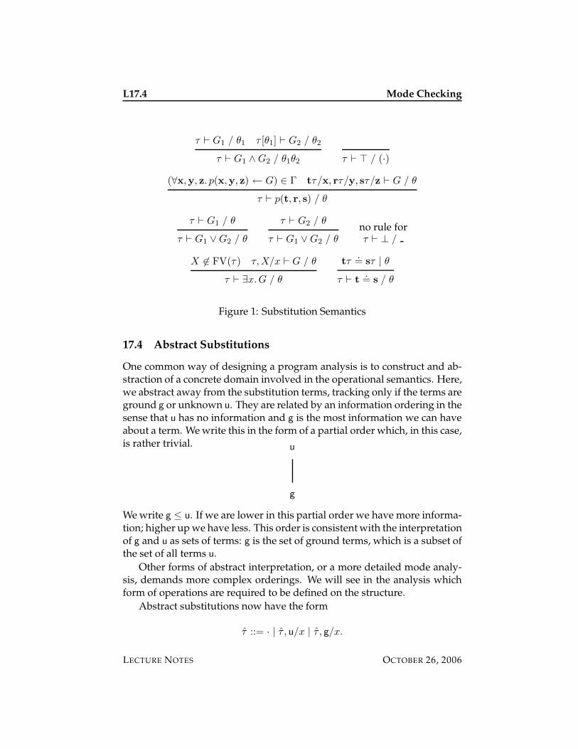
L17.4 Mode Checking
τ ` G1 / θ1 τ [θ1] ` G2 / θ2
τ ` G1 ∧G2 / θ1θ2 τ ` > / (·)
(∀x,y, z. p(x,y, z) ← G) ∈ Γ tτ/x, rτ/y, sτ/z ` G / θ
τ ` p(t, r, s) / θ
τ ` G1 / θ
τ ` G1 ∨G2 / θ
τ ` G2 / θ
τ ` G1 ∨G2 / θno rule forτ ` ⊥ /
X 6∈ FV(τ) τ,X/x ` G / θ
τ ` ∃x.G / θ
tτ.= sτ | θ
τ ` t.= s / θ
Figure 1: Substitution Semantics
17.4 Abstract Substitutions
One common way of designing a program analysis is to construct and ab-straction of a concrete domain involved in the operational semantics. Here,we abstract away from the substitution terms, tracking only if the terms areground g or unknown u. They are related by an information ordering in thesense that u has no information and g is the most information we can haveabout a term. We write this in the form of a partial order which, in this case,is rather trivial. u
g
We write g ≤ u. If we are lower in this partial order we have more informa-tion; higher up we have less. This order is consistent with the interpretationof g and u as sets of terms: g is the set of ground terms, which is a subset ofthe set of all terms u.
Other forms of abstract interpretation, or a more detailed mode analy-sis, demands more complex orderings. We will see in the analysis whichform of operations are required to be defined on the structure.
Abstract substitutions now have the form
τ ::= · | τ , u/x | τ , g/x.
LECTURE NOTES OCTOBER 26, 2006
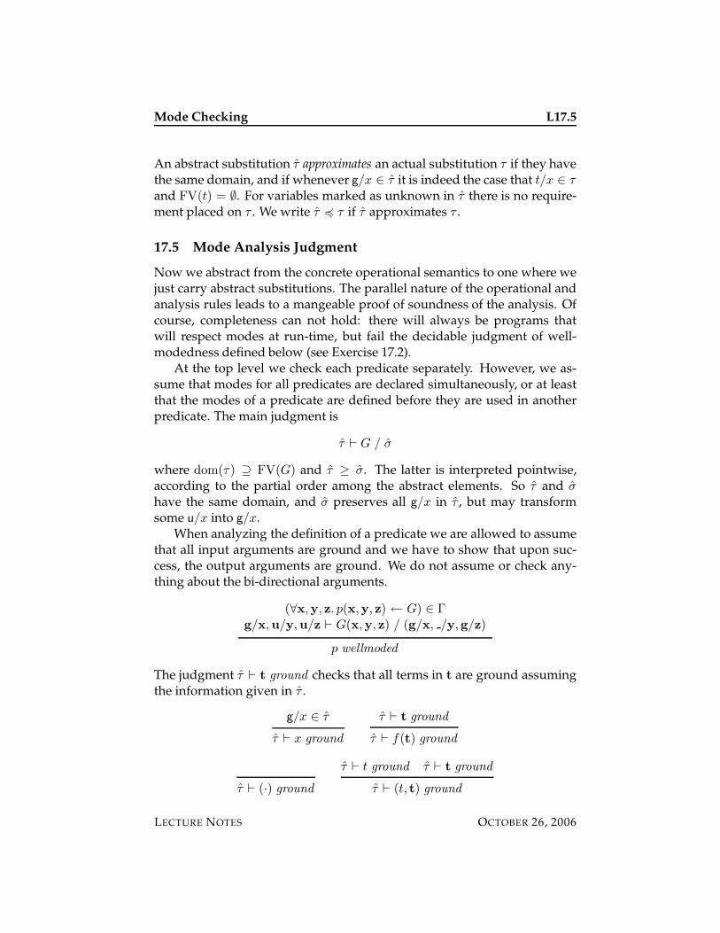
Mode Checking L17.5
An abstract substitution τ approximates an actual substitution τ if they havethe same domain, and if whenever g/x ∈ τ it is indeed the case that t/x ∈ τ
and FV(t) = ∅. For variables marked as unknown in τ there is no require-ment placed on τ . We write τ 4 τ if τ approximates τ .
17.5 Mode Analysis Judgment
Now we abstract from the concrete operational semantics to one where wejust carry abstract substitutions. The parallel nature of the operational andanalysis rules leads to a mangeable proof of soundness of the analysis. Ofcourse, completeness can not hold: there will always be programs thatwill respect modes at run-time, but fail the decidable judgment of well-modedness defined below (see Exercise 17.2).
At the top level we check each predicate separately. However, we as-sume that modes for all predicates are declared simultaneously, or at leastthat the modes of a predicate are defined before they are used in anotherpredicate. The main judgment is
τ ` G / σ
where dom(τ) ⊇ FV(G) and τ ≥ σ. The latter is interpreted pointwise,according to the partial order among the abstract elements. So τ and σ
have the same domain, and σ preserves all g/x in τ , but may transformsome u/x into g/x.
When analyzing the definition of a predicate we are allowed to assumethat all input arguments are ground and we have to show that upon suc-cess, the output arguments are ground. We do not assume or check any-thing about the bi-directional arguments.
(∀x,y, z. p(x,y, z) ← G) ∈ Γg/x,u/y,u/z ` G(x,y, z) / (g/x, /y,g/z)
p wellmoded
The judgment τ ` t ground checks that all terms in t are ground assumingthe information given in τ .
g/x ∈ τ
τ ` x ground
τ ` t ground
τ ` f(t) ground
τ ` (·) ground
τ ` t ground τ ` t ground
τ ` (t, t) ground
LECTURE NOTES OCTOBER 26, 2006
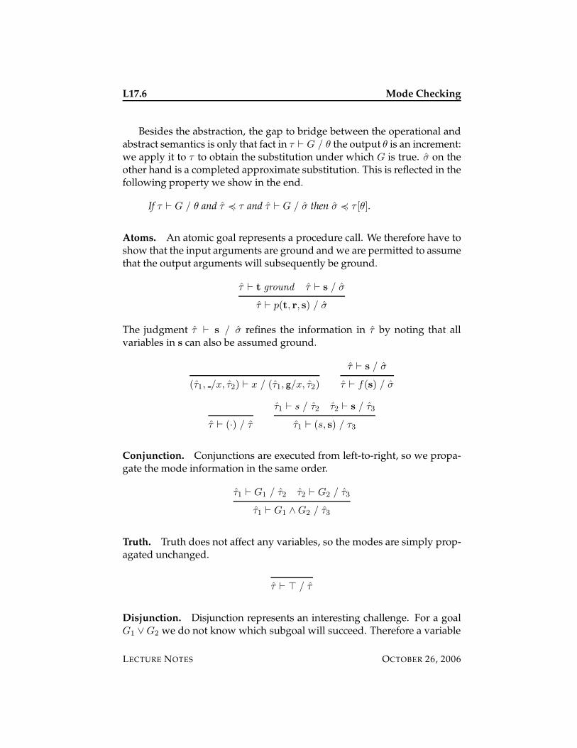
L17.6 Mode Checking
Besides the abstraction, the gap to bridge between the operational andabstract semantics is only that fact in τ ` G / θ the output θ is an increment:we apply it to τ to obtain the substitution under which G is true. σ on theother hand is a completed approximate substitution. This is reflected in thefollowing property we show in the end.
If τ ` G / θ and τ 4 τ and τ ` G / σ then σ 4 τ [θ].
Atoms. An atomic goal represents a procedure call. We therefore have toshow that the input arguments are ground and we are permitted to assumethat the output arguments will subsequently be ground.
τ ` t ground τ ` s / σ
τ ` p(t, r, s) / σ
The judgment τ ` s / σ refines the information in τ by noting that allvariables in s can also be assumed ground.
(τ1, /x, τ2) ` x / (τ1, g/x, τ2)
τ ` s / σ
τ ` f(s) / σ
τ ` (·) / τ
τ1 ` s / τ2 τ2 ` s / τ3
τ1 ` (s, s) / τ3
Conjunction. Conjunctions are executed from left-to-right, so we propa-gate the mode information in the same order.
τ1 ` G1 / τ2 τ2 ` G2 / τ3
τ1 ` G1 ∧G2 / τ3
Truth. Truth does not affect any variables, so the modes are simply prop-agated unchanged.
τ ` > / τ
Disjunction. Disjunction represents an interesting challenge. For a goalG1 ∨G2 we do not know which subgoal will succeed. Therefore a variable
LECTURE NOTES OCTOBER 26, 2006
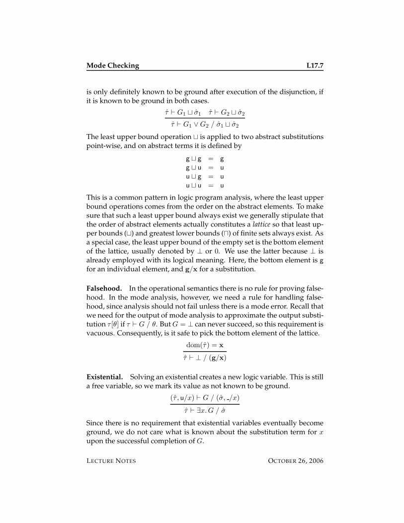
Mode Checking L17.7
is only definitely known to be ground after execution of the disjunction, ifit is known to be ground in both cases.
τ ` G1 t σ1 τ ` G2 t σ2
τ ` G1 ∨G2 / σ1 t σ2
The least upper bound operation t is applied to two abstract substitutionspoint-wise, and on abstract terms it is defined by
g t g = g
g t u = u
u t g = u
u t u = u
This is a common pattern in logic program analysis, where the least upperbound operations comes from the order on the abstract elements. To makesure that such a least upper bound always exist we generally stipulate thatthe order of abstract elements actually constitutes a lattice so that least up-per bounds (t) and greatest lower bounds (u) of finite sets always exist. Asa special case, the least upper bound of the empty set is the bottom elementof the lattice, usually denoted by ⊥ or 0. We use the latter because ⊥ isalready employed with its logical meaning. Here, the bottom element is g
for an individual element, and g/x for a substitution.
Falsehood. In the operational semantics there is no rule for proving false-hood. In the mode analysis, however, we need a rule for handling false-hood, since analysis should not fail unless there is a mode error. Recall thatwe need for the output of mode analysis to approximate the output substi-tution τ [θ] if τ ` G / θ. But G = ⊥ can never succeed, so this requirement isvacuous. Consequently, is it safe to pick the bottom element of the lattice.
dom(τ) = x
τ ` ⊥ / (g/x)
Existential. Solving an existential creates a new logic variable. This is stilla free variable, so we mark its value as not known to be ground.
(τ , u/x) ` G / (σ, /x)
τ ` ∃x.G / σ
Since there is no requirement that existential variables eventually becomeground, we do not care what is known about the substitution term for x
upon the successful completion of G.
LECTURE NOTES OCTOBER 26, 2006
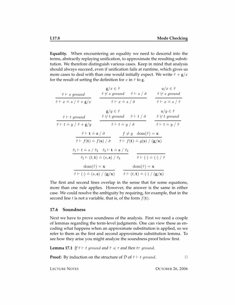
L17.8 Mode Checking
Equality. When encountering an equality we need to descend into theterms, abstractly replaying unification, to approximate the resulting substi-tution. We therefore distinguish various cases. Keep in mind that analysisshould always succeed, even if unification fails at runtime, which gives usmore cases to deal with than one would initially expect. We write τ + g/x
for the result of setting the definition for x in τ to g.
τ ` s ground
τ ` x.= s / τ + g/x
g/x ∈ τ
τ 6` s ground τ ` s / σ
τ ` x.= s / σ
u/x ∈ τ
τ 6` s ground
τ ` x.= s / τ
τ ` t ground
τ ` t.= y / τ + g/y
g/y ∈ τ
τ 6` t ground τ ` t / σ
τ ` t.= y / σ
u/y ∈ τ
τ 6` t ground
τ ` t.= y / τ
τ ` t.= s / σ
τ ` f(t).= f(s) / σ
f 6= g dom(τ) = x
τ ` f(t).= g(s) / (g/x)
τ1 ` t.= s / τ2 τ2 ` t
.= s / τ3
τ1 ` (t, t).= (s, s) / τ3 τ ` (·)
.= (·) / τ
dom(τ) = x
τ ` (·).= (s, s) / (g/x)
dom(τ) = x
τ ` (t, t).= (·) / (g/x)
The first and second lines overlap in the sense that for some equations,more than one rule applies. However, the answer is the same in eithercase. We could resolve the ambiguity by requiring, for example, that in thesecond line t is not a variable, that is, of the form f(t).
17.6 Soundness
Next we have to prove soundness of the analysis. First we need a coupleof lemmas regarding the term-level judgments. One can view these as en-coding what happens when an approximate substitution is applied, so werefer to them as the first and second approximate substitution lemma. Tosee how they arise you might analyze the soundness proof below first.
Lemma 17.1 If τ ` t ground and τ 4 τ and then tτ ground .
Proof: By induction on the structure of D of τ ` t ground . 2
LECTURE NOTES OCTOBER 26, 2006
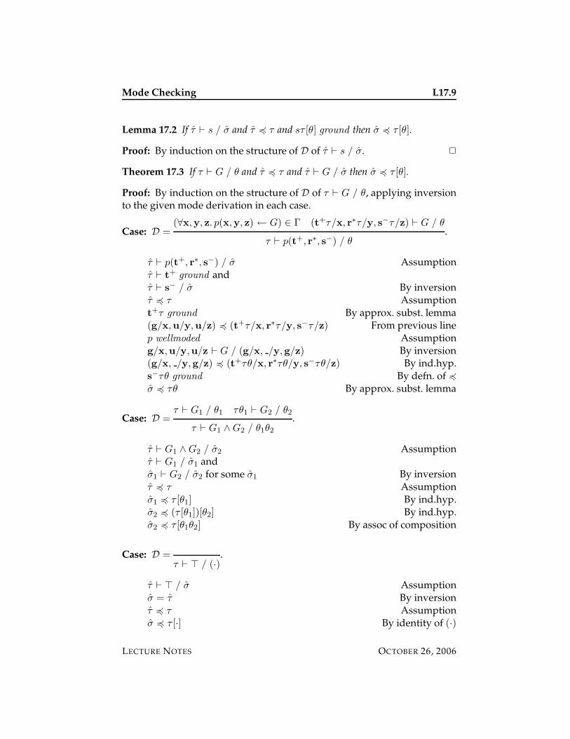
Mode Checking L17.9
Lemma 17.2 If τ ` s / σ and τ 4 τ and sτ [θ] ground then σ 4 τ [θ].
Proof: By induction on the structure of D of τ ` s / σ. 2
Theorem 17.3 If τ ` G / θ and τ 4 τ and τ ` G / σ then σ 4 τ [θ].
Proof: By induction on the structure of D of τ ` G / θ, applying inversionto the given mode derivation in each case.
Case: D =(∀x,y, z. p(x,y, z) ← G) ∈ Γ (t+τ/x, r∗τ/y, s−τ/z) ` G / θ
τ ` p(t+, r∗, s−) / θ.
τ ` p(t+, r∗, s−) / σ Assumptionτ ` t
+ ground andτ ` s
− / σ By inversionτ 4 τ Assumptiont+τ ground By approx. subst. lemma
(g/x,u/y,u/z) 4 (t+τ/x, r∗τ/y, s−τ/z) From previous linep wellmoded Assumptiong/x,u/y,u/z ` G / (g/x, /y,g/z) By inversion(g/x, /y,g/z) 4 (t+τθ/x, r∗τθ/y, s−τθ/z) By ind.hyp.s−τθ ground By defn. of 4
σ 4 τθ By approx. subst. lemma
Case: D =τ ` G1 / θ1 τθ1 ` G2 / θ2
τ ` G1 ∧G2 / θ1θ2
.
τ ` G1 ∧G2 / σ2 Assumptionτ ` G1 / σ1 andσ1 ` G2 / σ2 for some σ1 By inversionτ 4 τ Assumptionσ1 4 τ [θ1] By ind.hyp.σ2 4 (τ [θ1])[θ2] By ind.hyp.σ2 4 τ [θ1θ2] By assoc of composition
Case: D =τ ` > / (·)
.
τ ` > / σ Assumptionσ = τ By inversionτ 4 τ Assumptionσ 4 τ [·] By identity of (·)
LECTURE NOTES OCTOBER 26, 2006
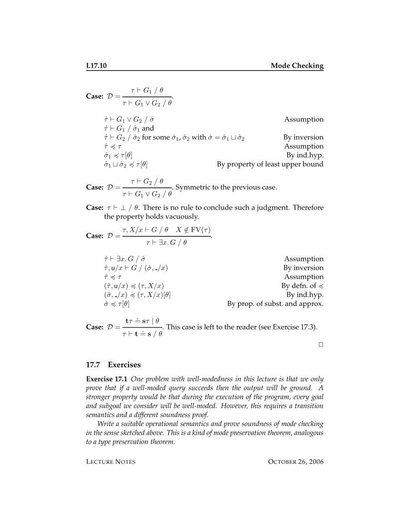
L17.10 Mode Checking
Case: D =τ ` G1 / θ
τ ` G1 ∨G2 / θ.
τ ` G1 ∨G2 / σ Assumptionτ ` G1 / σ1 andτ ` G2 / σ2 for some σ1, σ2 with σ = σ1 t σ2 By inversionτ 4 τ Assumptionσ1 4 τ [θ] By ind.hyp.σ1 t σ2 4 τ [θ] By property of least upper bound
Case: D =τ ` G2 / θ
τ ` G1 ∨G2 / θ. Symmetric to the previous case.
Case: τ ` ⊥ / θ. There is no rule to conclude such a judgment. Thereforethe property holds vacuously.
Case: D =τ,X/x ` G / θ X /∈ FV(τ)
τ ` ∃x.G / θ.
τ ` ∃x.G / σ Assumptionτ , u/x ` G / (σ, /x) By inversionτ 4 τ Assumption(τ , u/x) 4 (τ,X/x) By defn. of 4
(σ, /x) 4 (τ,X/x)[θ] By ind.hyp.σ 4 τ [θ] By prop. of subst. and approx.
Case: D =tτ
.= sτ | θ
τ ` t.= s / θ
. This case is left to the reader (see Exercise 17.3).
2
17.7 Exercises
Exercise 17.1 One problem with well-modedness in this lecture is that we onlyprove that if a well-moded query succeeds then the output will be ground. Astronger property would be that during the execution of the program, every goaland subgoal we consider will be well-moded. However, this requires a transitionsemantics and a different soundness proof.
Write a suitable operational semantics and prove soundness of mode checkingin the sense sketched above. This is a kind of mode preservation theorem, analogousto a type preservation theorem.
LECTURE NOTES OCTOBER 26, 2006
Mode Checking L17.11
Exercise 17.2 Give a program that respects modes at run-time in the sense that
• input arguments (+) are always ground when a predicate is invoked, and
• output arguments (-) are always ground when a predicate succeeds,
and yet is not well-moded according to our analysis.
Exercise 17.3 Complete the proof of soundness of mode analysis by giving the casefor unification. If you need a new lemma in addition to the approximate substitu-tion lemmas, carefully formulate and prove them.
LECTURE NOTES OCTOBER 26, 2006

L17.12 Mode Checking
LECTURE NOTES OCTOBER 26, 2006
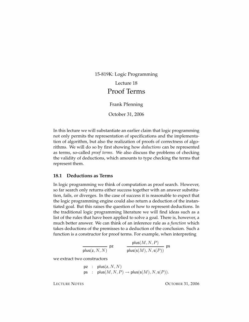
15-819K: Logic Programming
Lecture 18
Proof Terms
Frank Pfenning
October 31, 2006
In this lecture we will substantiate an earlier claim that logic programmingnot only permits the representation of specifications and the implementa-tion of algorithm, but also the realization of proofs of correctness of algo-rithms. We will do so by first showing how deductions can be representedas terms, so-called proof terms. We also discuss the problems of checkingthe validity of deductions, which amounts to type checking the terms thatrepresent them.
18.1 Deductions as Terms
In logic programming we think of computation as proof search. However,so far search only returns either success together with an answer substitu-tion, fails, or diverges. In the case of success it is reasonable to expect thatthe logic programming engine could also return a deduction of the instan-tiated goal. But this raises the question of how to represent deductions. Inthe traditional logic programming literature we will find ideas such as alist of the rules that have been applied to solve a goal. There is, however, amuch better answer. We can think of an inference rule as a function whichtakes deductions of the premisses to a deduction of the conclusion. Such afunction is a constructor for proof terms. For example, when interpreting
plus(z, N,N)pz
plus(M,N,P )
plus(s(M),N, s(P ))ps
we extract two constructors
pz : plus(z,N,N)ps : plus(M,N,P )→ plus(s(M),N, s(P )).
LECTURE NOTES OCTOBER 31, 2006
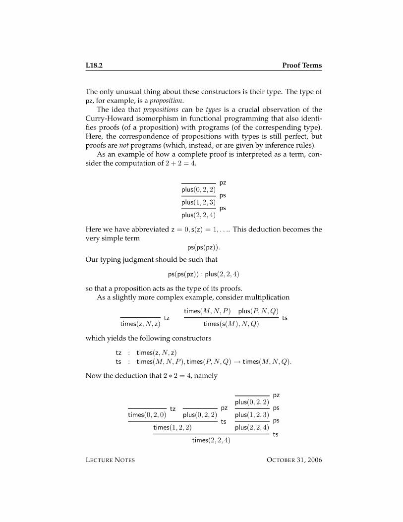
L18.2 Proof Terms
The only unusual thing about these constructors is their type. The type ofpz, for example, is a proposition.
The idea that propositions can be types is a crucial observation of theCurry-Howard isomorphism in functional programming that also identi-fies proofs (of a proposition) with programs (of the correspending type).Here, the correspondence of propositions with types is still perfect, butproofs are not programs (which, instead, or are given by inference rules).
As an example of how a complete proof is interpreted as a term, con-sider the computation of 2 + 2 = 4.
plus(0, 2, 2)pz
plus(1, 2, 3)ps
plus(2, 2, 4)ps
Here we have abbreviated z = 0, s(z) = 1, . . .. This deduction becomes thevery simple term
ps(ps(pz)).
Our typing judgment should be such that
ps(ps(pz)) : plus(2, 2, 4)
so that a proposition acts as the type of its proofs.As a slightly more complex example, consider multiplication
times(z, N, z)tz
times(M,N,P ) plus(P,N,Q)
times(s(M),N,Q)ts
which yields the following constructors
tz : times(z, N, z)ts : times(M,N,P ), times(P,N,Q)→ times(M,N,Q).
Now the deduction that 2 ∗ 2 = 4, namely
times(0, 2, 0)tz
plus(0, 2, 2)pz
times(1, 2, 2)ts
plus(0, 2, 2)pz
plus(1, 2, 3)ps
plus(2, 2, 4)ps
times(2, 2, 4)ts
LECTURE NOTES OCTOBER 31, 2006
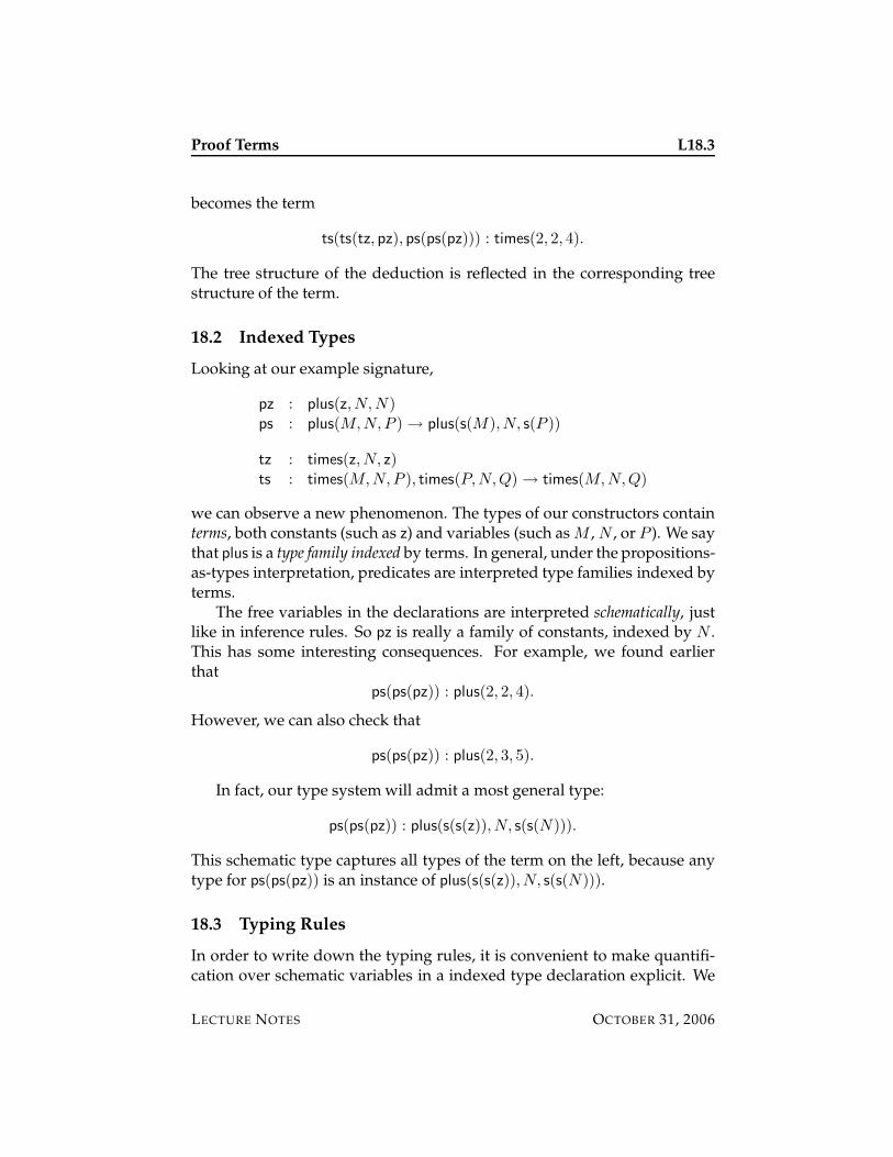
Proof Terms L18.3
becomes the term
ts(ts(tz, pz), ps(ps(pz))) : times(2, 2, 4).
The tree structure of the deduction is reflected in the corresponding treestructure of the term.
18.2 Indexed Types
Looking at our example signature,
pz : plus(z, N,N)ps : plus(M,N,P )→ plus(s(M),N, s(P ))
tz : times(z, N, z)ts : times(M,N,P ), times(P,N,Q)→ times(M,N,Q)
we can observe a new phenomenon. The types of our constructors containterms, both constants (such as z) and variables (such as M , N , or P ). We saythat plus is a type family indexed by terms. In general, under the propositions-as-types interpretation, predicates are interpreted type families indexed byterms.
The free variables in the declarations are interpreted schematically, justlike in inference rules. So pz is really a family of constants, indexed by N .This has some interesting consequences. For example, we found earlierthat
ps(ps(pz)) : plus(2, 2, 4).
However, we can also check that
ps(ps(pz)) : plus(2, 3, 5).
In fact, our type system will admit a most general type:
ps(ps(pz)) : plus(s(s(z)),N, s(s(N))).
This schematic type captures all types of the term on the left, because anytype for ps(ps(pz)) is an instance of plus(s(s(z)),N, s(s(N))).
18.3 Typing Rules
In order to write down the typing rules, it is convenient to make quantifi-cation over schematic variables in a indexed type declaration explicit. We
LECTURE NOTES OCTOBER 31, 2006
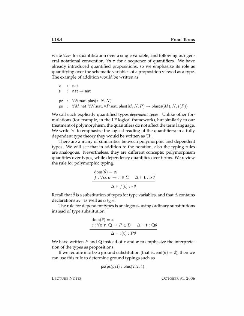
L18.4 Proof Terms
write ∀x:τ for quantification over a single variable, and following our gen-eral notational convention, ∀x:τ for a sequence of quantifiers. We havealready introduced quantified propositions, so we emphasize its role asquantifying over the schematic variables of a proposition viewed as a type.The example of addition would be written as
z : nat
s : nat→ nat
pz : ∀N :nat. plus(z, N,N)ps : ∀M :nat.∀N :nat.∀P :nat. plus(M,N,P )→ plus(s(M),N, s(P ))
We call such explicitly quantified types dependent types. Unlike other for-mulations (for example, in the LF logical framework), but similarly to ourtreatment of polymorphism, the quantifiers do not affect the term language.We write ‘∀’ to emphasize the logical reading of the quantifiers; in a fullydependent type theory they would be written as ‘Π’.
There are a many of similarities between polymorphic and dependenttypes. We will see that in addition to the notation, also the typing rulesare analogous. Nevertheless, they are different concepts: polymorphismquantifies over types, while dependency quantifies over terms. We reviewthe rule for polymorphic typing.
dom(θ) = α
f : ∀α.σ → τ ∈ Σ ∆ ` t : σθ
∆ ` f(t) : τ θ
Recall that θ is a substitution of types for type variables, and that ∆ containsdeclarations x:τ as well as α type .
The rule for dependent types is analogous, using ordinary substitutionsinstead of type substitution.
dom(θ) = x
c : ∀x:τ .Q→ P ∈ Σ ∆ ` t : Qθ
∆ ` c(t) : Pθ
We have written P and Q instead of τ and σ to emphasize the interpreta-tion of the types as propositions.
If we require θ to be a ground substitution (that is, cod(θ) = ∅), then wecan use this rule to determine ground typings such as
ps(ps(pz)) : plus(2, 2, 4).
LECTURE NOTES OCTOBER 31, 2006

Proof Terms L18.5
If we allow free variables, that is, cod(θ) = dom(∆), then we can write outschematic typings, such as
n:nat ` ps(ps(pz)) : plus(s(s(z)), n, s(s(n))).
In either case we want the substitution to be well-typed. In the presence ofdependent types, the formalization of this would lead us a bit far afield, sowe can think of it just as before: we always substitute a term of type τ for avariable of type τ .
18.4 Type Checking
Ordinarily in logic programming a query is simply a proposition and theresult is an answer substitution for its free variables. When we have proofterms we can also ask if a given term constitutes a proof of a given propo-sition. We might write this as
?- t : P.
where t is a term representing a purported proof and P is a goal proposi-tion. From the typing rule we can see that type-checking comes down tounification. We can make this more explicit by rewriting the rule:
dom(ρ) = x
c : ∀x:τ .Q→ P ′ ∈ Σ P ′ρ.= P | θ ∆ ` t : Qρθ
∆ ` c(t) : P
Here ρ is a renaming substituting generating fresh logic variables for thebound variables x.
Because a constant has at most one declaration in a signature, and uni-fication returns a unique most general unifier, the type-checking process isentirely deterministic and will always either fail (in which case there is notype) or succeed. We can even leave P as a variable and obtain the mostgeneral type for a given term t.
Checking that a given term represents a valid proof can be useful in anumber of situations. Some practical scenarios where this has been appliedis proof-carrying code and proof-carrying authorization. Proof-carrying code isthe idea that we can equip a piece of mobile code with a proof that it issafe to execute. A code recipient can check the validity of the proof againstthe code and then run the code without further run-time checks. Proof-carrying authorization is a similar idea, except that the proof is used to
LECTURE NOTES OCTOBER 31, 2006
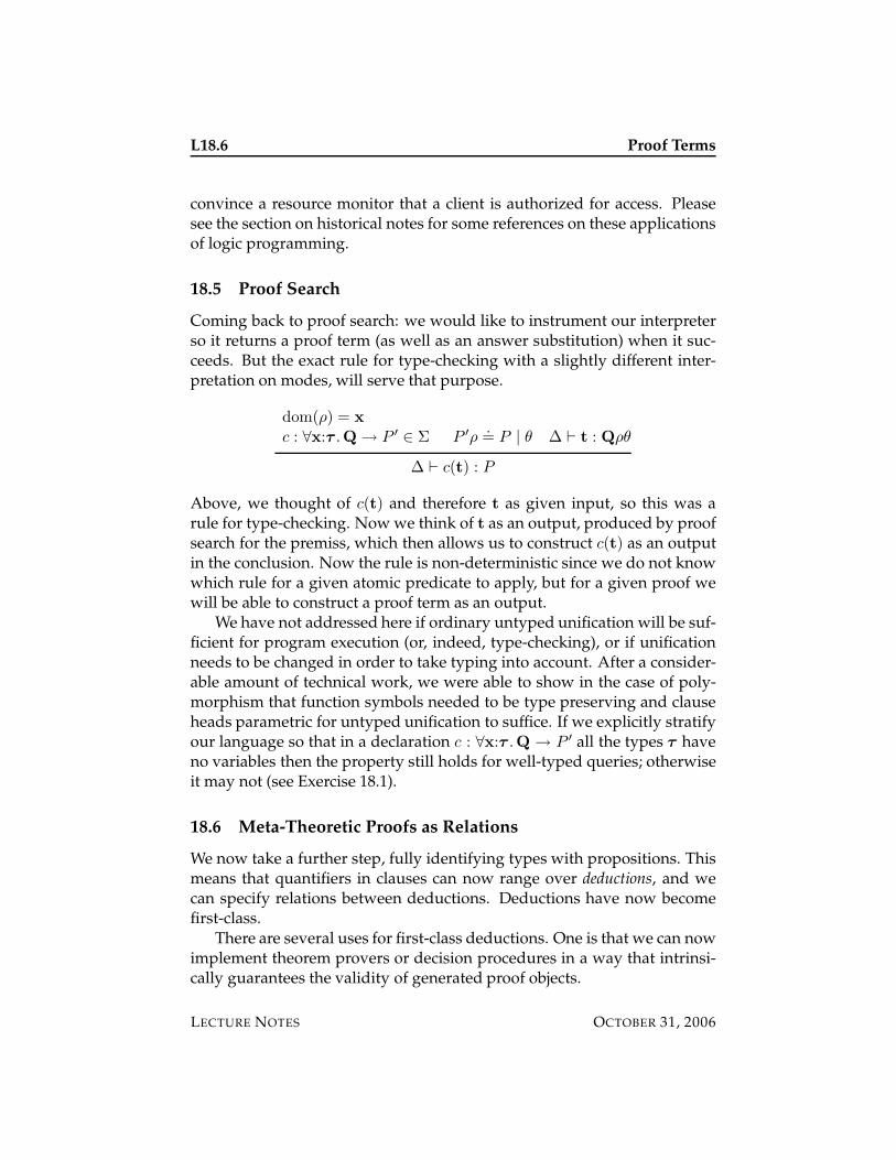
L18.6 Proof Terms
convince a resource monitor that a client is authorized for access. Pleasesee the section on historical notes for some references on these applicationsof logic programming.
18.5 Proof Search
Coming back to proof search: we would like to instrument our interpreterso it returns a proof term (as well as an answer substitution) when it suc-ceeds. But the exact rule for type-checking with a slightly different inter-pretation on modes, will serve that purpose.
dom(ρ) = x
c : ∀x:τ .Q→ P ′ ∈ Σ P ′ρ.= P | θ ∆ ` t : Qρθ
∆ ` c(t) : P
Above, we thought of c(t) and therefore t as given input, so this was arule for type-checking. Now we think of t as an output, produced by proofsearch for the premiss, which then allows us to construct c(t) as an outputin the conclusion. Now the rule is non-deterministic since we do not knowwhich rule for a given atomic predicate to apply, but for a given proof wewill be able to construct a proof term as an output.
We have not addressed here if ordinary untyped unification will be suf-ficient for program execution (or, indeed, type-checking), or if unificationneeds to be changed in order to take typing into account. After a consider-able amount of technical work, we were able to show in the case of poly-morphism that function symbols needed to be type preserving and clauseheads parametric for untyped unification to suffice. If we explicitly stratifyour language so that in a declaration c : ∀x:τ .Q → P ′ all the types τ haveno variables then the property still holds for well-typed queries; otherwiseit may not (see Exercise 18.1).
18.6 Meta-Theoretic Proofs as Relations
We now take a further step, fully identifying types with propositions. Thismeans that quantifiers in clauses can now range over deductions, and wecan specify relations between deductions. Deductions have now becomefirst-class.
There are several uses for first-class deductions. One is that we can nowimplement theorem provers or decision procedures in a way that intrinsi-cally guarantees the validity of generated proof objects.
LECTURE NOTES OCTOBER 31, 2006
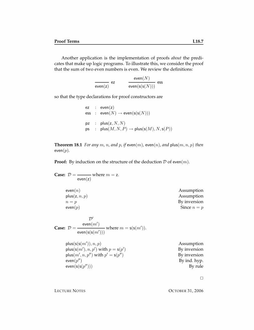
Proof Terms L18.7
Another application is the implementation of proofs about the predi-cates that make up logic programs. To illustrate this, we consider the proofthat the sum of two even numbers is even. We review the definitions:
even(z)ez
even(N)
even(s(s(N)))ess
so that the type declarations for proof constructors are
ez : even(z)ess : even(N)→ even(s(s(N)))
pz : plus(z,N,N)ps : plus(M,N,P )→ plus(s(M),N, s(P ))
Theorem 18.1 For any m, n, and p, if even(m), even(n), and plus(m,n, p) theneven(p).
Proof: By induction on the structure of the deduction D of even(m).
Case: D =even(z)
where m = z.
even(n) Assumptionplus(z, n, p) Assumptionn = p By inversioneven(p) Since n = p
Case: D =
D′
even(m′)
even(s(s(m′)))where m = s(s(m′)).
plus(s(s(m′)), n, p) Assumptionplus(s(m′), n, p′) with p = s(p′) By inversionplus(m′, n, p′′) with p′ = s(p′′) By inversioneven(p′′) By ind. hyp.even(s(s(p′′))) By rule
2
LECTURE NOTES OCTOBER 31, 2006
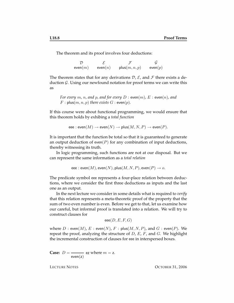
L18.8 Proof Terms
The theorem and its proof involves four deductions:
Deven(m)
Eeven(n)
Fplus(m,n, p)
G
even(p)
The theorem states that for any derivations D, E , and F there exists a de-duction G. Using our newfound notation for proof terms we can write thisas
For every m, n, and p, and for every D : even(m), E : even(n), andF : plus(m,n, p) there exists G : even(p).
If this course were about functional programming, we would ensure thatthis theorem holds by exhibing a total function
eee : even(M)→ even(N)→ plus(M,N,P )→ even(P ).
It is important that the function be total so that it is guaranteed to generatean output deduction of even(P ) for any combination of input deductions,thereby witnessing its truth.
In logic programming, such functions are not at our disposal. But wecan represent the same information as a total relation
eee : even(M), even(N), plus(M,N,P ), even(P )→ o.
The predicate symbol eee represents a four-place relation between deduc-tions, where we consider the first three deductions as inputs and the lastone as an output.
In the next lecture we consider in some details what is required to verifythat this relation represents a meta-theoretic proof of the property that thesum of two even number is even. Before we get to that, let us examine howour careful, but informal proof is translated into a relation. We will try toconstruct clauses for
eee(D,E,F,G)
where D : even(M), E : even(N), F : plus(M,N,P ), and G : even(P ). Werepeat the proof, analyzing the structure of D, E, F , and G. We highlightthe incremental construction of clauses for eee in interspersed boxes.
Case: D =even(z)
ez where m = z.
LECTURE NOTES OCTOBER 31, 2006
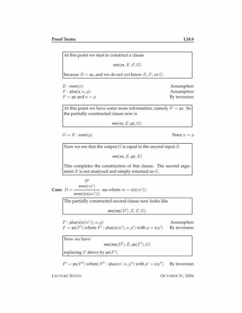
Proof Terms L18.9
At this point we start to construct a clause
eee(ez, E, F,G)
because D = ez, and we do not yet know E, F , or G.
E : even(n) AssumptionF : plus(z, n, p) AssumptionF = pz and n = p By inversion
At this point we have some more information, namely F = pz. Sothe partially constructed clause now is
eee(ez, E, pz, G).
G = E : even(p) Since n = p
Now we see that the output G is equal to the second input E.
eee(ez, E, pz, E)
This completes the construction of this clause. The second argu-ment E is not analyzed and simply returned as G.
Case: D =
D′
even(m′)
even(s(s(m′)))ess where m = s(s(m′)).
The partially constructed second clause now looks like
eee(ess(D′), E, F,G).
F : plus(s(s(m′)), n, p) AssumptionF = ps(F ′) where F ′ : plus(s(m′), n, p′) with p = s(p′) By inversion
Now we haveeee(ess(D′), E, ps(F ′), G)
replacing F above by ps(F ′).
F ′ = ps(F ′′) where F ′′ : plus(m′, n, p′′) with p′ = s(p′′) By inversion
LECTURE NOTES OCTOBER 31, 2006
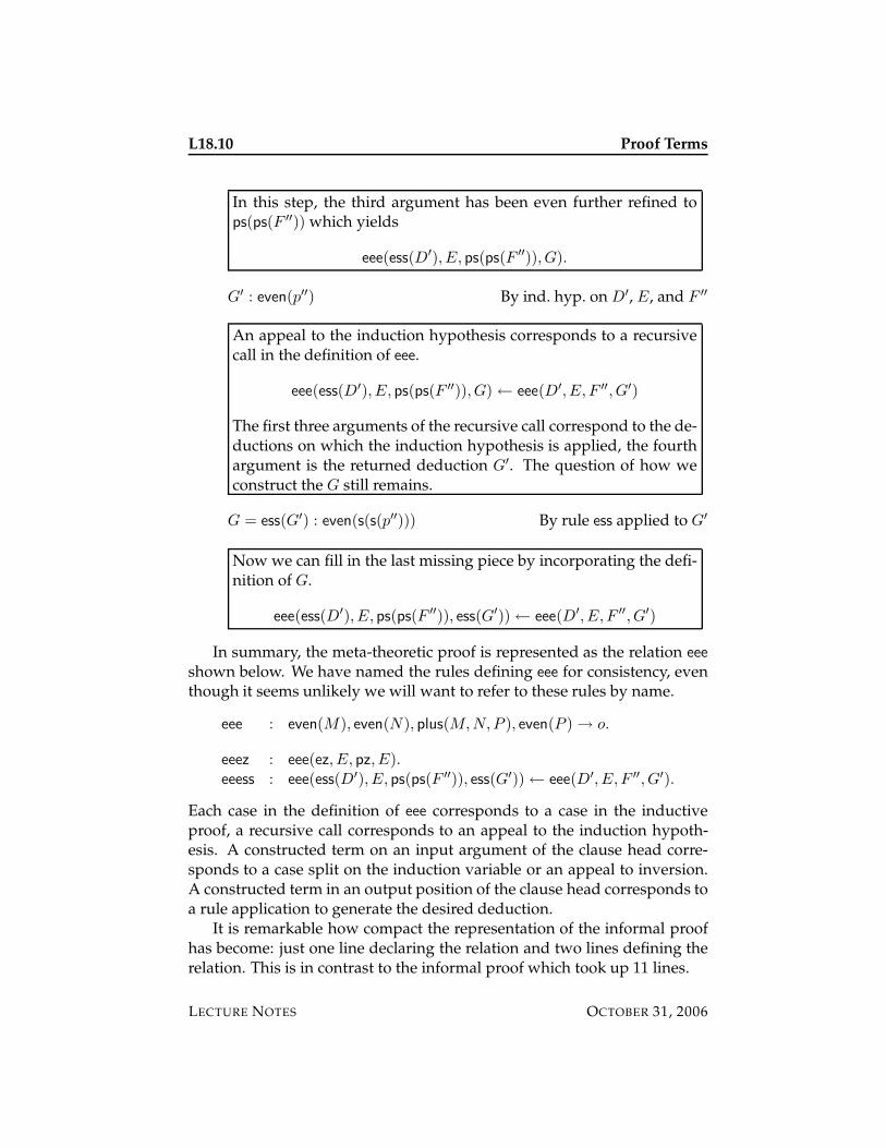
L18.10 Proof Terms
In this step, the third argument has been even further refined tops(ps(F ′′)) which yields
eee(ess(D′), E, ps(ps(F ′′)), G).
G′ : even(p′′) By ind. hyp. on D′, E, and F ′′
An appeal to the induction hypothesis corresponds to a recursivecall in the definition of eee.
eee(ess(D′), E, ps(ps(F ′′)), G)← eee(D′, E, F ′′, G′)
The first three arguments of the recursive call correspond to the de-ductions on which the induction hypothesis is applied, the fourthargument is the returned deduction G′. The question of how weconstruct the G still remains.
G = ess(G′) : even(s(s(p′′))) By rule ess applied to G′
Now we can fill in the last missing piece by incorporating the defi-nition of G.
eee(ess(D′), E, ps(ps(F ′′)), ess(G′))← eee(D′, E, F ′′, G′)
In summary, the meta-theoretic proof is represented as the relation eee
shown below. We have named the rules defining eee for consistency, eventhough it seems unlikely we will want to refer to these rules by name.
eee : even(M), even(N), plus(M,N,P ), even(P )→ o.
eeez : eee(ez, E, pz, E).eeess : eee(ess(D′), E, ps(ps(F ′′)), ess(G′))← eee(D′, E, F ′′, G′).
Each case in the definition of eee corresponds to a case in the inductiveproof, a recursive call corresponds to an appeal to the induction hypoth-esis. A constructed term on an input argument of the clause head corre-sponds to a case split on the induction variable or an appeal to inversion.A constructed term in an output position of the clause head corresponds toa rule application to generate the desired deduction.
It is remarkable how compact the representation of the informal proofhas become: just one line declaring the relation and two lines defining therelation. This is in contrast to the informal proof which took up 11 lines.
LECTURE NOTES OCTOBER 31, 2006
Proof Terms L18.11
18.7 Verifying Proofs of Meta-Theorems
In the previous section we showed how to represent a proof of a theoremabout deductions as a relation between proofs. But what does it take toverify that a given relation indeed represents a meta-theoretic proof of aproposed theorem? A full treatment of this question is beyond the scope ofthis lecture (and probably this course), but meta-logical frameworks suchas Twelf can indeed verify this. Twelf decomposes this checking into mul-tiple steps, each making its own contribution to the overall verification.
1. Type checking. This guarantees that if eee(D,E,F,G) for deductionsD, E, F , and G is claimed, all of these are valid deductions. In partic-ular, the output G will be acceptable evidence that P is even becauseG : even(P ).
2. Mode checking. The mode eee(+,+,+,−) guarantees that if the in-puts are all complete (ground) deductions and the query succeeds,then the output is also a complete (ground) deduction. This is impor-tant because a free variable in a proof term represents an unprovensubgoal. Such deductions would be insufficient as evidence that P isindeed even.
3. Totality checking. If type checking and mode checking succeeds, weknow that P is even if a query eee(D,E,F,G) succeeds for groundD, E, F and free variable G. All that remains is to show that all suchqueries succeed. We decompose this into two properties.
(a) Progress checking. For any given combination of input deduc-tions D, E, and F there is an applicable clause and we eithersucceed or at least can proceed to a subgoal. Because of this,eee(D,E,F,G) can never fail.
(b) Termination checking. Any sequence of recursive calls will ter-minate. Since queries can not fail (by progress) the only remain-ing possibility is that they succeed, which is what we needed toverify.
We have already extensively discussed type checking and mode check-ing. In the next lecture we sketch progress checking. For termination check-ing we refer to the literature in the historical notes below.
LECTURE NOTES OCTOBER 31, 2006
L18.12 Proof Terms
18.8 Polymorphism and Dependency
Because of the similarity of polymorphic and dependent types, and becauseboth have different uses, it is tempting to combine the two in a single lan-guage. This is indeed possible. For example, if we would like to index apolymorphic list with its length we could define
nat : type.
z : nat.
s : nat -> nat.
list : type,nat -> type.
nil : list(A,z).
cons : A,list(A,N) -> list(A,s(N)).
In the setting of functional programming, such combinations have beenthoroughly investigated, for examples, as fragments of the Calculus of Con-structions. In the setting here we are not aware of a thorough study of eithertype checking or unification. A tricky issue seems to be how much type in-formation must be carried at run-time, during unification, especially if atype variable can be instantiated by a dependent type.
18.9 Historical Notes
The notion of proof term originates in the so-called Curry-Howard iso-morphism, which was noted for combinatory logic by Curry and Feys in1956 [8] and for natural deduction by Howard in 1969 [10]. The empha-sis in this work is on functional computation, by combinatory reductionor β-reduction, respectively. The presentation here is much closer to theLF logical framework [9] in which only canonical forms are relevant, andwhich is entirely based on dependent types. We applied one main sim-plification: because we restricted ourselves to the Horn fragment of logic,proof terms contain no λ-abstractions. This in turn allows us to omit Π-quantifiers without any loss of decidability of type checking, since typeinference can be achieved just by ordinary unification.
The combination of polymorphism and dependency is present in theCalculus of Constructions [6]. Various fragments were later analyzed indetail by Barendregt [2], including the combination of polymorphism withdependent types. A modern version of the Calculus of Constructions is thebasis for the Coq theorem proving system.1
1http://coq.inria.fr/
LECTURE NOTES OCTOBER 31, 2006
Proof Terms L18.13
The use of explicit proof terms to certify the safety of mobile code goesback to Necula and Lee [13, 12]. They used the LF logical framework withsome optimizations for proof representation. Proof-carrying authorizationwas proposed by Appel and Felten [1] and then realized for the first timeby Bauer, Schneider, and Felten [5, 3]. It is now one of the cornerstonesof the Grey project [4] for universal distributed access control at CarnegieMellon University.
The technique of representing proofs of meta-theorems by relations ismy own work [14, 15], eventually leading to the Twelf system [17] whichhas many contributors. Type reconstruction for Twelf was already sketchedin the early work [15], followed the first foray into mode checking andtermination checking [19] later extended by Pientka [18]. Totality check-ing [21] was a further development of meta-proofs that were correct byconstruction proposed by Schurmann [20]. The example in this lecture canbe easily verified in Twelf. For more on Twelf see the Twelf home page.2
Relational representation of meta-theory has recently been shown to besufficiently powerful to mechanize the theory of full-scale programminglanguages (Typed Assembly Language [7] and Standard ML [11]). Forfurther references and a more general introduction to logical frameworks,see [16].
18.10 Exercises
Exercise 18.1 We can translate the conditions on polymorphism, namely that thatterm constructors be type-preserving and predicates be parametric, to conditionson dependency. Give such a parallel definition.
Further, give examples that show the need for type information to be carriedduring unification to avoid creating ill-typed terms if these conditions are violated.
Finally, discuss which of these, if any, would be acceptable in the case of depen-dent types.
Exercise 18.2 Revisit the proof that the empty list is the right unit for append
(Exercise 3.5 from Assignment 2) and represent it formally as a relation betweendeductions.
Exercise 18.3 Revisit the proof that addition is commutative (Exercise 3.4 fromAssignment 2) and represent it formally as a relation between deductions.
Exercise 18.4 Revisit the proof that append is associative (Exercise 3.6 from As-signment 2) and represent it formally as a relation between deductions.
2http://www.twelf.org/
LECTURE NOTES OCTOBER 31, 2006
L18.14 Proof Terms
Exercise 18.5 If we do not want to change the logic programming engine to pro-duce proof objects, we can transform a program globally by adding an additionalargument to every predicate, denoting a proof term.
Formally define this transformation and prove its correctness.
18.11 References
[1] Andrew W. Appel and Edward W. Felten. Proof-carrying authentica-tion. In G. Tsudik, editor, Proceedings of the 6th Conference on Computerand Communications Security, pages 52–62, Singapore, November 1999.ACM Press.
[2] Henk P. Barendregt. Lambda calculi with types. In S. Abramsky,D. Gabbay, and T.S.E. Maibaum, editors, Handbook of Logic in ComputerScience, volume 2, chapter 2, pages 117–309. Oxford University Press,1992.
[3] Lujo Bauer. Access Control for the Web via Proof-Carrying Authorization.PhD thesis, Princeton University, November 2003.
[4] Lujo Bauer, Scott Garriss, Jonathan M. McCune, Michael K. Reiter, Ja-son Rouse, and Peter Rutenbar. Device-enabled authorization in theGrey system. In Proceedings of the 8th Information Security Conference(ISC’05), pages 431–445, Singapore, September 2005. Springer VerlagLNCS 3650.
[5] Lujo Bauer, Michael A. Schneider, and Edward W. Felten. A generaland flexible access-control system for the web. In Proceedings of the11th USENIX Security Symposium, San Francisco, California, August2002.
[6] Thierry Coquand and Gerard Huet. The calculus of constructions. In-formation and Computation, 76(2/3):95–120, 1988.
[7] Karl Crary and Susmit Sarkar. Foundational certified code in a meta-logical framework. ACM Transactions on Computational Logic, 2006. Toappear.
[8] H. B. Curry and R. Feys. Combinatory Logic. North-Holland, Amster-dam, 1958.
[9] Robert Harper, Furio Honsell, and Gordon Plotkin. A frameworkfor defining logics. Journal of the Association for Computing Machinery,40(1):143–184, January 1993.
LECTURE NOTES OCTOBER 31, 2006
Proof Terms L18.15
[10] W. A. Howard. The formulae-as-types notion of construction. In J. P.Seldin and J. R. Hindley, editors, To H. B. Curry: Essays on CombinatoryLogic, Lambda Calculus and Formalism, pages 479–490. Academic Press,1980. Hitherto unpublished note of 1969, rearranged, corrected, andannotated by Howard.
[11] Daniel K. Lee, Karl Crary, and Robert Harper. Mechanizing themetatheory of Standard ML. Technical Report CMU-CS-06-138, Car-negie Mellon University, 2006.
[12] George C. Necula. Proof-carrying code. In Neil D. Jones, editor, Con-ference Record of the 24th Symposium on Principles of Programming Lan-guages (POPL’97), pages 106–119, Paris, France, January 1997. ACMPress.
[13] George C. Necula and Peter Lee. Safe kernel extensions without run-time checking. In Proceedings of the Second Symposium on OperatingSystem Design and Implementation (OSDI’96), pages 229–243, Seattle,Washington, October 1996.
[14] Frank Pfenning. Elf: A language for logic definition and verified meta-programming. In Fourth Annual Symposium on Logic in Computer Sci-ence, pages 313–322, Pacific Grove, California, June 1989. IEEE Com-puter Society Press.
[15] Frank Pfenning. Logic programming in the LF logical framework. InGerard Huet and Gordon Plotkin, editors, Logical Frameworks, pages149–181. Cambridge University Press, 1991.
[16] Frank Pfenning. Logical frameworks. In Alan Robinson and AndreiVoronkov, editors, Handbook of Automated Reasoning, chapter 17, pages1063–1147. Elsevier Science and MIT Press, 2001.
[17] Frank Pfenning and Carsten Schurmann. System description: Twelf— a meta-logical framework for deductive systems. In H. Ganzinger,editor, Proceedings of the 16th International Conference on Automated De-duction (CADE-16), pages 202–206, Trento, Italy, July 1999. Springer-Verlag LNAI 1632.
[18] Brigitte Pientka and Frank Pfenning. Termination and reductionchecking in the logical framework. In Carsten Schurmann, editor,Workshop on Automation of Proofs by Mathematical Induction, Pittsburgh,Pennsylvania, June 2000.
[19] Ekkehard Rohwedder and Frank Pfenning. Mode and terminationchecking for higher-order logic programs. In Hanne Riis Nielson, edi-
LECTURE NOTES OCTOBER 31, 2006
L18.16 Proof Terms
tor, Proceedings of the European Symposium on Programming, pages 296–310, Linkoping, Sweden, April 1996. Springer-Verlag LNCS 1058.
[20] Carsten Schurmann. Automating the Meta Theory of Deductive Systems.PhD thesis, Department of Computer Science, Carnegie Mellon Uni-versity, August 2000. Available as Technical Report CMU-CS-00-146.
[21] Carsten Schurmann and Frank Pfenning. A coverage checking al-gorithm for LF. In D. Basin and B. Wolff, editors, Proceedings of the16th International Conference on Theorem Proving in Higher Order Logics(TPHOLs 2003), pages 120–135, Rome, Italy, September 2003. Springer-Verlag LNCS 2758.
LECTURE NOTES OCTOBER 31, 2006
15-819K: Logic Programming
Lecture 19
Verifying Progress
Frank Pfenning
November 2, 2006
In this lecture we discuss another logic program analysis, namely verify-ing the progress property. Progress guarantees that a predicate can neverfail for arbitrary values of its input arguments. Together with terminationthis guarantees that a predicate is total in its given input arguments. Assketched in the previous lecture, this an important piece in the general tech-nique of verifying properties of logic programs by reasoning about proofterms.
19.1 The Progress Property
Progress in general just says that during the execution of a program wehave either finished computation with a value, or we can make a furtherstep. In particular, computation can never “get stuck”. In logic program-ming this translates to saying the computation can never fail. This requiresan understanding of the intended input and output arguments of a predi-cate, as well as the domain on which it is to be applied.
Returning to the well-worn example of addition,
plus(z, N,N).plus(s(M),N, s(P )) ← plus(M,N,P ).
the plus predicate is total in the first two arguments, assuming they are nat-ural numbers. It is not total in the first and third argument, because a querysuch as plus(s(z), N, z) will fail. Totality decomposes into two subquestions,namely progress and termination, since we always assume the program iswell-typed and well-moded. Termination is easy to see here because the
LECTURE NOTES NOVEMBER 2, 2006
L19.2 Verifying Progress
first argument decreases strictly in each recursive call. Progress is also easyto see because the first argument must be a natural number, and thereforebe either of the form z or s(m) for some m, and the second argument can beanything because both clause heads have a variable in that position.
Even though the principal application of progress is probably the ver-ification of proof of metatheorems presented in relational form, progresscan also be used to check that some given predicates are total functions (al-though ruling out multi-valued functions requires another step). This mayprovide the programmer with additional confidence that no cases in thedefinition of a logic program were missed.
19.2 The Right Semantic Starting Point
As repeatedly emphasized, finding the right semantic starting point for ananalysis is the key to obtaining a simple, predictable system and the easiestproof of correctness. For progress, the residuated form of the program issomewhat difficult to deal with. Consider the simple form of plus(+,+,−)above (easily seen to satisfy progress) and the residuated form
plus(x1, x2, x3)← (∃N.x1
.= z ∧ x2
.= N ∧ x2
.= N)
∨ (∃M.∃N.∃P. x1
.= s(M) ∧ x2
.= N ∧ x3
.= s(P ) ∧ plus(M,N,P ))
on which it is more difficult to discern the same property. Moreover, failureplays no role in the progress property because, in fact, it is never permittedto occur, so the semantics should not need to carry a failure continuation.
Hence we return to a fairly early semantics, in which the subgoal stackis explicit, but not the failure continuation. On the other hand, the substi-tution for the variables is crucial, so we make that explicit. Recall that thereis a fixed program Γ with a set of closed clauses.
τ ` G1 / G2 ∧ S
τ ` G1 ∧G2 / S
τ ` G2 / S
τ ` > / G2 ∧ S τ ` > / >
(∀x. P ′ ← G) ∈ Γ P ′ρ.= Pτ | θ τθ, ρθ ` G / S
τ ` P / S
In the last rule, ρ is a substitution renaming x to a new set of logic variablesX, that is, dom(ρ) = x, cod(ρ) ∩ cod(τ) = ∅. We also assume that thevariables x have been renamed so that x ∩ dom(τ) = ∅.
From this semantics it is easily seen that progress is a question regard-ing atomic goals, because the cases for conjunction and truth always apply.
LECTURE NOTES NOVEMBER 2, 2006
Verifying Progress L19.3
19.3 Input and Output Coverage
Focusing in, we rewrite the rules for predicate calls assuming the predicatep(t, s) has a mode declaration which divides the arguments into input ar-guments t, which come first, and output arguments s, which come second.
(∀x. p(t′, s′)← G) ∈ Γ (t′ρ, s′ρ).= (tτ, sτ) | θ τθ, ρθ ` G / S
τ ` p(t, s) / S
We have ensured progress if such a clause and unifier θ always exist.Breaking it down a bit further, we see we must have
There exists a θ such that (1) t′ρθ = tτθ, and (2) s
′ρθ = sτθ wheret′ are the input terms in the clause head, s′ are the output terms in the
clause head, t are the input arguments to the predicate call, and s arethe output arguments in the predicate call.
We refer to part (1) as input coverage and part (2) as output coverage. Inthe problem analysis above a single substitution θ is required, but we willapproximate this by two separate checks. In the next two sections we willdescribe the analysis for the two parts of coverage checking. We previewthem here briefly.
For input coverage we need to recall the assumption that predicates arewell-moded. This means that the input arguments in the call, tτθ will beground. Hence input coverage is satisfied if for any sequence t of groundterms of the right types, there exists a clause head such that its input argu-ments t
′ can be instantiated to t.Output coverage is trickier. The problem is that mode analysis does not
tell us anything about the output argument sτ of the call p(tτ, sτ). What weknow if that if p succeeds with substitution τθ′, then sτθ′ will be ground,but this does not help. From examples, like plus above, we can observe thatoutput coverage is satisfied because the output argument of the call (in thesecond clause for plus it is P ) is a variable, and will remain a variable untilthe call is made. This means we have to sharpen mode checking to verifythat some variables remain free, which we tackle below.
19.4 Input Coverage
Given a program Γ and a predicate p : (τ ,σ) → o with input argumentsof type τ . We say that p satisfies input coverage in Γ if for any sequence ofground terms t : τ there exists a clause ∀x:τ ′. p(t′, s′) ← G and a substitu-tion θ : (x:τ ′) such that t
′θ = t.
LECTURE NOTES NOVEMBER 2, 2006
L19.4 Verifying Progress
For the description of the algorithm, we will need a slightly more gen-eral form. We write ∆ ` Γp � t (read: Γp immediately covers t) if thereexists a clause ∀x:τ ′. p(t′, s′) ← G in Γp and a substitution ∆ ` θ : (x : τ
′)such that t
′θ = t. We write ∆ ` Γp > t (read: Γp covers t) if for everyground instance tσ with σ : ∆ there exists a clause ∀x:τ ′. p(t′, s) ← G inΓp and a subsitution ∆ ` θ : (x:τ ′) such that t
′θ = tσ. Clearly, immediatecoverage implies coverage, but not vice versa.
We reconsider the plus predicate, with the first two arguments consid-ered as inputs.
plus(z, N,N).plus(s(M),N, s(P )) ← plus(M,N,P ).
By the preceding remark, in order to show that input coverage holds, it issufficient to show that
x1:nat, x2:nat ` Γplus > (x1, x2).
Clearly, immediate coverage does not hold, because x1 is not an instance ofeither z or s(M). On the other hand, x2 is an instance of N .
At this point we need to exploit the assumption x1:nat by applying anappropriate left rule. This is acceptable because we move from the usualopen world assumption (any predicate and type is inherently open-ended)to the closed world assumption (all predicates and types are given com-pletely by their definition). The closed world assumption is necessary be-cause progress (and coverage) can only be establish with respect to a fixedset of types and clauses and could immediately be violated by new decla-rations (e.g., the additional declaration ω : nat causes input coverage forplus to fail).
To see what the left rules would look like, we can take a short detourthrough type predicates. The declarations
z : nat.
s : nat→ nat.
correspond tonat(z).nat(s(N))← nat(N).
The iff-completion yields
nat(N) ↔ N.= z ∨ ∃N ′.N
.= s(N ′) ∧ nat(N ′).
LECTURE NOTES NOVEMBER 2, 2006
Verifying Progress L19.5
The left rule for nat(x) (which is not the most general case, but sufficient forour purposes) for an arbitrary judgment J on the right-hand side can thenbe derived as
` J(z/x)
x.= z ` J
nat(x′) ` J(s(x′)/x)
x.= s(x′) ∧ nat(x′) ` J
∃N ′. x.= s(N ′) ∧ nat(N ′) ` J
x.= z ∨ ∃N ′. x
.= s(N ′) ∧ nat(N ′) ` J
nat(x) ` J
or, in summary:` J(z/x) nat(x′) ` J(s(x′)/x)
nat(x) ` J
Translated back to types:
∆ ` J(z/x) ∆, x′:nat ` J(s(x′)/x)
∆, x:nat ` J
Using this rule, we can now prove our goal:
x2:nat ` Γplus > (z, x2) x′
1:nat, x2:nat ` Γplus > (s(x′
1), x2)
x1:nat, x2:nat ` Γplus > (x1, x2)
Both of the premisses now follow by immediate coverage, using the firstclause for the first premiss and the second clause for the second premiss,using the critical rule
∆ ` Γp � t
∆ ` Γp > t
For immediate coverage, there is but one rule.
(∀x:τ ′. p(t′, s′)← G) ∈ Γp t′θ = t for ∆ ` θ : (x:τ ′)
∆ ` Γp � t
We do not write out the left rules, but it should be clear how to derive themfrom the type declarations, at least for simple types. We call this processsplitting of a variable x:τ .
An interesting aspect of the left rules is that they are asynchronous.However, always applying them leads to non-termination, so we have tofollow some terminating strategy. This strategy can be summarized infor-mally as follows, given a goal ∆ ` Γp > t.
LECTURE NOTES NOVEMBER 2, 2006
L19.6 Verifying Progress
1. Check if ∆ ` Γp � t. If so, succeed.
2. If not, pick a variable x:τ in ∆ and apply inversion as sketched above.This yields a collection of subgoals ∆i ` Γp � ti. Solve each subgoal.
Picking the right variable to split is crucial for termination. Briefly, we picka variable x that was involved in a clash f(t′′)
.= x when attempting imme-
diate coverage, where f(t′′) is a subterm of t′. Now one of the possibilities
for x will have f as it top-level function symbol, reducing the clash the nexttime around. Thus the splitting process is bounded by the total size of theinput terms in Γp. See the reference below for further discussion and proofof this fact.
19.5 Output Coverage
Output coverage is to ensure that for every goal p(t, s) encountered whileexecuting a program, the output positions s
′ of the relevant clause headp(t′, s′) are an instance of s (if t and t
′ unify). The problem is that ordinarymode checking does not tell us anything about s: we do not know whetherit will be ground or partially ground or consist of all free variables. How-ever, if we knew that s consisted of pairwise distinct free variables whenthe goal p(t, s) arose, then output coverage would be satisfied since thevariables in s cannot occur in a clause head and therefore the unificationprocess must succeed.
So we can guarantee output coverage with a sharpened mode-checkingprocess where an output arguments must be distinct free variables whena predicate is invoked. Moreover, they must become ground by the timethe predicate suceeds. This is actually very easy: just change the abstractdomain of the mode analysis from u > g (unknown and ground) to f > g
(free and ground). If we also have bidirectional arguments in addition toinput and output we three abstract values with f > u > g. The remainderof the development is just as in a previous lecture (see Exercise 19.1). Theonly slightly tricky aspect is that the output arguments must be distinct freevariables, otherwise the individual substitutions may not compose to onefor all output arguments simultaneously.
Returning to our example,
plus(z, N,N).plus(s(M),N, s(P )) ← plus(M,N,P ).
the only output argument is P , which is indeed a free variable when thatsubgoal is executed.
LECTURE NOTES NOVEMBER 2, 2006
Verifying Progress L19.7
We show a couple of cases for failure of output coverage, to illustratesome points. Assume we have already checked progress for plus. The pro-gram
test← plus(z, z, s(P )).
trivially satisfies input coverage, but yet fails (and hence cannot satisfyprogress). This is because the output argument in the only call is s(P ),which is not a free variable. This will be noted by the sharpened modechecker.
Similarly, the program
test←
plus(z, s(z), P ),plus(s(z), s(z), P ).
trivially satisfies input coverage but it does not pass the sharpened modechecker because the second occurrence of P will be ground (from the firstcall) rather than free when the second subgoal is executed. And, indeed,plus will fail and hence cannot satisfy progress.
Finally, a the predicate nexttwo(+,−,−)
nexttwo(N, s(N), s(s(N))).
satisfies progress, but
test← nexttwo(s(z), P, P ).
does not, because the two occurrences of P would have to be s(s(z)) ands(s(s(z))) simultaneously.
19.6 Historical Notes
Progress and coverage do not appear to have received much attention inthe logic programming literature, possibly because they requires types tobe interesting, and their main application lies in verifying proofs of meta-theorems which is a recent development. An algorithm for coverage in thericher setting with dependent types is given by Schurmann and myself [1],which also contains some pointers to earlier literature in functional pro-gramming.
LECTURE NOTES NOVEMBER 2, 2006
L19.8 Verifying Progress
19.7 Exercises
Exercise 19.1 Write out the rules for a sharpened mode checker with only inputand output arguments where output arguments must be distinct free variableswhen a predicate is invoked.
19.8 References
[1] Carsten Schurmann and Frank Pfenning. A coverage checking algo-rithm for LF. In D. Basin and B. Wolff, editors, Proceedings of the 16th In-ternational Conference on Theorem Proving in Higher Order Logics (TPHOLs2003), pages 120–135, Rome, Italy, September 2003. Springer-VerlagLNCS 2758.
LECTURE NOTES NOVEMBER 2, 2006
15-819K: Logic Programming
Lecture 20
Bottom-Up Logic Programming
Frank Pfenning
November 7, 2006
In this lecture we return to the view that a logic program is defined by acollection of inference rules for atomic propositions. But we now base theoperational semantics on reasoning forward from facts, which are initiallygiven as rules with no premisses. Every rule application potentially addsnew facts. Whenever no more new facts can be generated we say forwardreasoning saturates and we can answer questions about truth by examiningthe saturated database of facts. We illustrate bottom-up logic program-ming with several programs, including graph reachability, CKY parsing,and liveness analysis.
20.1 Bottom-Up Inference
We now return the very origins of logic programming as an operationalinterpretation of inference rules defining atomic predicates. As a reminder,consider the definition of even.
even(z)evz
even(N)
even(s(s(N)))evss
This works very well on queries such as even(s(s(s(s(z))))) (which succeeds)and even(s(s(s(z)))) (which fails). In fact, the operational reading of thisprogram under goal-directed search constitutes a decision procedure forground queries even(n).
This specification makes little sense under an alternative interpretationwhere we eagerly apply the inference rules in the forward direction, fromthe premisses to the conclusion, until no new facts can be deduced. The
LECTURE NOTES NOVEMBER 7, 2006
L20.2 Bottom-Up Logic Programming
problem is that we start with even(z), then obtain even(s(s(z))), and so on,but we never terminate.
It would be too early to give up on forward reasoning at this point. Aswe have seen many times, even in backward reasoning a natural specifica-tion of a predicate does not necessarily lead to a reasonable implementa-tion. We can implement a test whether a number is even via reasoning bycontradication. We seed our database with the claim that n is not even andderive consequences from that assumption. If we derive a contradictoryfact we know thate even(n) must be true. If not (and our rules are com-plete), then even(n) must be false. We write odd(n) for the proposition thatn is not even. Then we obtain the following specification
odd(s(s(N)))
odd(N)
to be used for forward reasoning. This single rule obviously saturates be-cause the argument to odd becomes smaller in every rule application.
What is not formally represented in this program is how we initial-ize our database (we assume odd(n)), and how we interpret the saturateddatabase (we check if odd(z) was deduced). In a later lecture we will seethat it is possible to combine forward and backward reasoning to makesthose aspects of an algorithm also part of its implementation.
The strategy of this example, proof by contradiction, does not alwayswork, but there are many cases where it does. One should check if thepredicate is decidable as a first test. We will see further examples later,specifically the treatment of unification in the next lecture.
20.2 Graph Reachability
Assuming we have a specification of edge(x, y) whenever there is an edgefrom node x to node y, we can specify reachability path(x, y) with the rules
edge(X,Y )
path(X,Y )
edge(X,Y ) path(Y,Z)
path(X,Z)
During bottom-up inference these rules will saturate when they have con-structed the transitive closure of the edge relation. During backward rea-soning these rules may not terminate (if there are cycles), or be very ineffi-cient (if there are many paths compared to the number of nodes).
In the forward direction the rules will always saturate. We can also give,just from the rules, a complexity analysis of the saturation algorithm.
LECTURE NOTES NOVEMBER 7, 2006
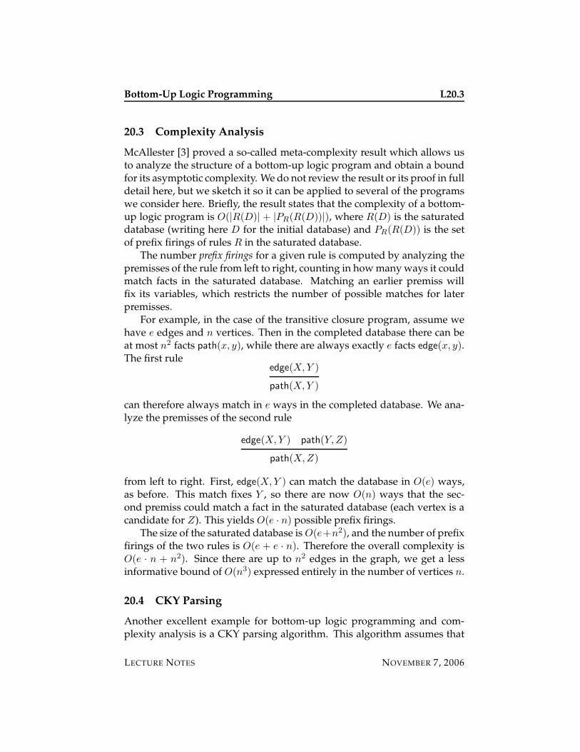
Bottom-Up Logic Programming L20.3
20.3 Complexity Analysis
McAllester [3] proved a so-called meta-complexity result which allows usto analyze the structure of a bottom-up logic program and obtain a boundfor its asymptotic complexity. We do not review the result or its proof in fulldetail here, but we sketch it so it can be applied to several of the programswe consider here. Briefly, the result states that the complexity of a bottom-up logic program is O(|R(D)| + |PR(R(D))|), where R(D) is the saturateddatabase (writing here D for the initial database) and PR(R(D)) is the setof prefix firings of rules R in the saturated database.
The number prefix firings for a given rule is computed by analyzing thepremisses of the rule from left to right, counting in how many ways it couldmatch facts in the saturated database. Matching an earlier premiss willfix its variables, which restricts the number of possible matches for laterpremisses.
For example, in the case of the transitive closure program, assume wehave e edges and n vertices. Then in the completed database there can beat most n2 facts path(x, y), while there are always exactly e facts edge(x, y).The first rule
edge(X,Y )
path(X,Y )
can therefore always match in e ways in the completed database. We ana-lyze the premisses of the second rule
edge(X,Y ) path(Y,Z)
path(X,Z)
from left to right. First, edge(X,Y ) can match the database in O(e) ways,as before. This match fixes Y , so there are now O(n) ways that the sec-ond premiss could match a fact in the saturated database (each vertex is acandidate for Z). This yields O(e · n) possible prefix firings.
The size of the saturated database is O(e+n2), and the number of prefixfirings of the two rules is O(e + e · n). Therefore the overall complexity isO(e · n + n2). Since there are up to n2 edges in the graph, we get a lessinformative bound of O(n3) expressed entirely in the number of vertices n.
20.4 CKY Parsing
Another excellent example for bottom-up logic programming and com-plexity analysis is a CKY parsing algorithm. This algorithm assumes that
LECTURE NOTES NOVEMBER 7, 2006
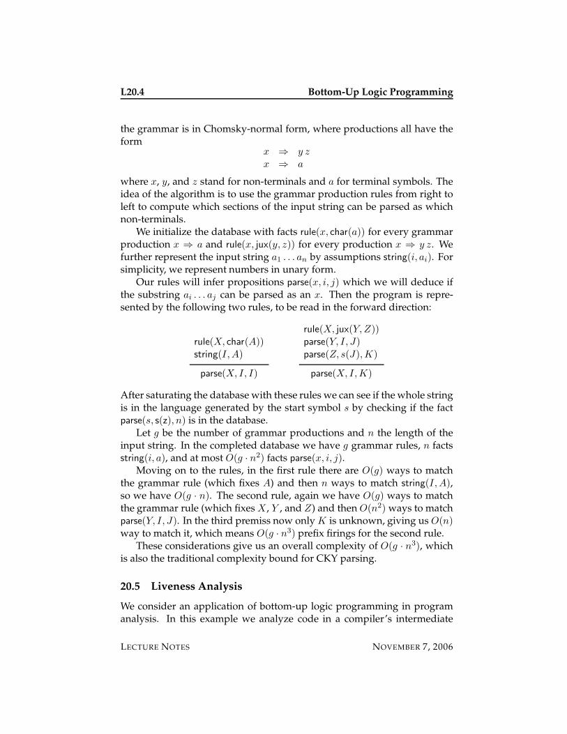
L20.4 Bottom-Up Logic Programming
the grammar is in Chomsky-normal form, where productions all have theform
x ⇒ y z
x ⇒ a
where x, y, and z stand for non-terminals and a for terminal symbols. Theidea of the algorithm is to use the grammar production rules from right toleft to compute which sections of the input string can be parsed as whichnon-terminals.
We initialize the database with facts rule(x, char(a)) for every grammarproduction x ⇒ a and rule(x, jux(y, z)) for every production x ⇒ y z. Wefurther represent the input string a1 . . . an by assumptions string(i, ai). Forsimplicity, we represent numbers in unary form.
Our rules will infer propositions parse(x, i, j) which we will deduce ifthe substring ai . . . aj can be parsed as an x. Then the program is repre-sented by the following two rules, to be read in the forward direction:
rule(X, char(A))string(I,A)
parse(X, I, I)
rule(X, jux(Y,Z))parse(Y, I, J)parse(Z, s(J),K)
parse(X, I,K)
After saturating the database with these rules we can see if the whole stringis in the language generated by the start symbol s by checking if the factparse(s, s(z), n) is in the database.
Let g be the number of grammar productions and n the length of theinput string. In the completed database we have g grammar rules, n factsstring(i, a), and at most O(g · n2) facts parse(x, i, j).
Moving on to the rules, in the first rule there are O(g) ways to matchthe grammar rule (which fixes A) and then n ways to match string(I,A),so we have O(g · n). The second rule, again we have O(g) ways to matchthe grammar rule (which fixes X, Y , and Z) and then O(n2) ways to matchparse(Y, I, J). In the third premiss now only K is unknown, giving us O(n)way to match it, which means O(g · n3) prefix firings for the second rule.
These considerations give us an overall complexity of O(g · n3), whichis also the traditional complexity bound for CKY parsing.
20.5 Liveness Analysis
We consider an application of bottom-up logic programming in programanalysis. In this example we analyze code in a compiler’s intermediate
LECTURE NOTES NOVEMBER 7, 2006
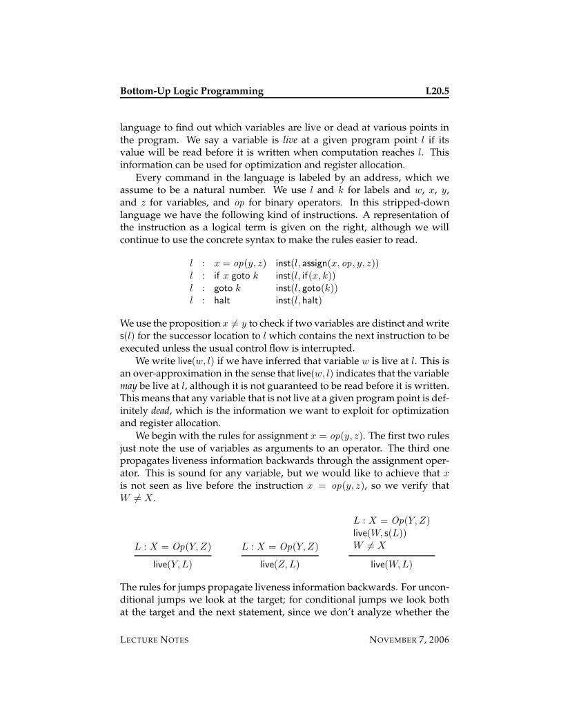
Bottom-Up Logic Programming L20.5
language to find out which variables are live or dead at various points inthe program. We say a variable is live at a given program point l if itsvalue will be read before it is written when computation reaches l. Thisinformation can be used for optimization and register allocation.
Every command in the language is labeled by an address, which weassume to be a natural number. We use l and k for labels and w, x, y,and z for variables, and op for binary operators. In this stripped-downlanguage we have the following kind of instructions. A representation ofthe instruction as a logical term is given on the right, although we willcontinue to use the concrete syntax to make the rules easier to read.
l : x = op(y, z) inst(l, assign(x, op, y, z))l : if x goto k inst(l, if(x, k))l : goto k inst(l, goto(k))l : halt inst(l, halt)
We use the proposition x 6= y to check if two variables are distinct and writes(l) for the successor location to l which contains the next instruction to beexecuted unless the usual control flow is interrupted.
We write live(w, l) if we have inferred that variable w is live at l. This isan over-approximation in the sense that live(w, l) indicates that the variablemay be live at l, although it is not guaranteed to be read before it is written.This means that any variable that is not live at a given program point is def-initely dead, which is the information we want to exploit for optimizationand register allocation.
We begin with the rules for assignment x = op(y, z). The first two rulesjust note the use of variables as arguments to an operator. The third onepropagates liveness information backwards through the assignment oper-ator. This is sound for any variable, but we would like to achieve that x
is not seen as live before the instruction x = op(y, z), so we verify thatW 6= X.
L : X = Op(Y,Z)
live(Y,L)
L : X = Op(Y,Z)
live(Z,L)
L : X = Op(Y,Z)live(W, s(L))W 6= X
live(W,L)
The rules for jumps propagate liveness information backwards. For uncon-ditional jumps we look at the target; for conditional jumps we look bothat the target and the next statement, since we don’t analyze whether the
LECTURE NOTES NOVEMBER 7, 2006
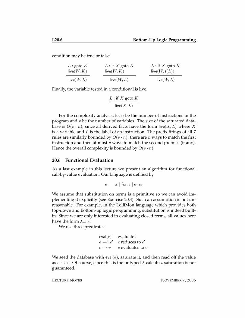
L20.6 Bottom-Up Logic Programming
condition may be true or false.
L : goto K
live(W,K)
live(W,L)
L : if X goto K
live(W,K)
live(W,L)
L : if X goto K
live(W, s(L))
live(W,L)
Finally, the variable tested in a conditional is live.
L : if X goto K
live(X,L)
For the complexity analysis, let n be the number of instructions in theprogram and v be the number of variables. The size of the saturated data-base is O(v · n), since all derived facts have the form live(X,L) where X
is a variable and L is the label of an instruction. The prefix firings of all 7rules are similarly bounded by O(v · n): there are n ways to match the firstinstruction and then at most v ways to match the second premiss (if any).Hence the overall complexity is bounded by O(v · n).
20.6 Functional Evaluation
As a last example in this lecture we present an algorithm for functionalcall-by-value evaluation. Our language is defined by
e ::= x | λx. e | e1 e2
We assume that substitution on terms is a primitive so we can avoid im-plementing it explicitly (see Exercise 20.4). Such an assumption is not un-reasonable. For example, in the LolliMon language which provides bothtop-down and bottom-up logic programming, substitution is indeed built-in. Since we are only interested in evaluating closed terms, all values herehave the form λx. e.
We use three predicates:
eval(e) evaluate e
e →∗ e′ e reduces to e′
e ↪→ v e evaluates to v.
We seed the database with eval(e), saturate it, and then read off the valueas e ↪→ v. Of course, since this is the untyped λ-calculus, saturation is notguaranteed.
LECTURE NOTES NOVEMBER 7, 2006
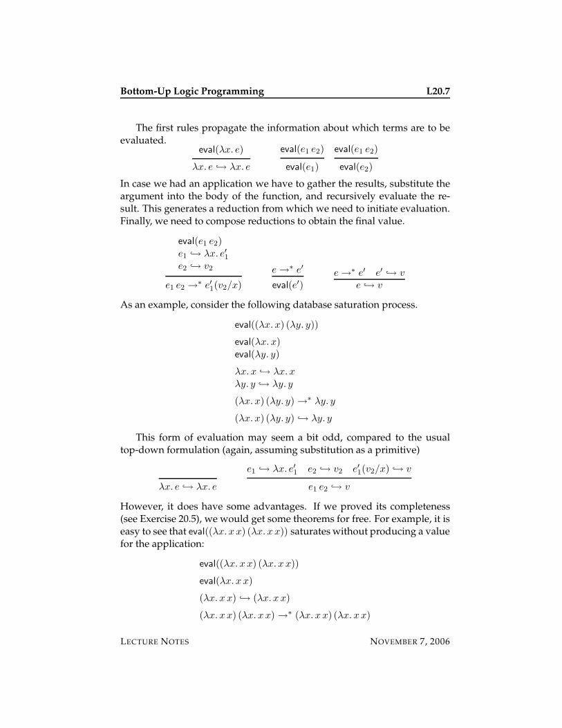
Bottom-Up Logic Programming L20.7
The first rules propagate the information about which terms are to beevaluated.
eval(λx. e)
λx. e ↪→ λx. e
eval(e1 e2)
eval(e1)
eval(e1 e2)
eval(e2)
In case we had an application we have to gather the results, substitute theargument into the body of the function, and recursively evaluate the re-sult. This generates a reduction from which we need to initiate evaluation.Finally, we need to compose reductions to obtain the final value.
eval(e1 e2)e1 ↪→ λx. e′
1
e2 ↪→ v2
e1 e2 →∗ e′1(v2/x)
e →∗ e′
eval(e′)e →∗ e′ e′ ↪→ v
e ↪→ v
As an example, consider the following database saturation process.
eval((λx. x) (λy. y))
eval(λx. x)eval(λy. y)
λx. x ↪→ λx. x
λy. y ↪→ λy. y
(λx. x) (λy. y) →∗ λy. y
(λx. x) (λy. y) ↪→ λy. y
This form of evaluation may seem a bit odd, compared to the usualtop-down formulation (again, assuming substitution as a primitive)
λx. e ↪→ λx. e
e1 ↪→ λx. e′1
e2 ↪→ v2 e′1(v2/x) ↪→ v
e1 e2 ↪→ v
However, it does have some advantages. If we proved its completeness(see Exercise 20.5), we would get some theorems for free. For example, it iseasy to see that eval((λx. x x) (λx. x x)) saturates without producing a valuefor the application:
eval((λx. x x) (λx. x x))
eval(λx. x x)
(λx. x x) ↪→ (λx. x x)
(λx. x x) (λx. x x) →∗ (λx. x x) (λx. x x)
LECTURE NOTES NOVEMBER 7, 2006
L20.8 Bottom-Up Logic Programming
At this point the database is saturated. This proves that the evaluation of(λx. x x) (λx. x x) fails. In the top-down semantics (that is, with backwardchaining as in Prolog), such a query would fail to terminate instead unlesswe added some kind of loop detection.
Note that the bottom-up program for evaluation, which consists of sixrules, cannot be analyzed with McAllester’s technique, because in the con-clusion of the rule for reduction a new term e′
1(v2/x) is created. We can
therefore not bound the size of the completed database. And, in fact, thesaturation may fail to terminate (see Exercise 20.7).
20.7 Variable Restrictions
Bottom-up logic programming, as considered by McAllester, requires thatevery variable in the conclusion of a rule also appears in a premiss. Thismeans that every generated fact will be ground. This is important for sat-uration and complexity analysis because a fact with a free variable couldstand for infinitely many instances.
Nonetheless, bottom-up logic programming can be generalized in thepresence of free variables and we will do this in a later lecture.
20.8 Historical Notes
The bottom-up interpretation of logic programs goes back to the early daysof logic programming. See, for example, the paper by Naughton and Ra-makrishnan [4].
There are at least three areas were logic programming specification witha bottom-up semantics has found significant applications: deductive data-bases, decision procedures, and program analysis. Unification, as presentin the next lecture, is an example of a decision procedure for unifiability.Liveness analysis is an example of program analysis due to McAllester [3],who was particularly interested in describing program analysis algorithmsat a high level of abstraction so their complexity would be self-evident. Thiswas later refined by Ganzinger and McAllester [1, 2] by allowing deletionsin the database. We treat this in a later lecture where we generalize bottom-up inference to linear logic.
20.9 Exercises
Exercise 20.1 Write a bottom-up logic program for addition (plus/3) on num-bers in unary form and then extend it to multiplication (times/3).
LECTURE NOTES NOVEMBER 7, 2006
Bottom-Up Logic Programming L20.9
Exercise 20.2 Consider the following variant of graph reachability.
edge(X,Y )
path(X,Y )
path(X,Y ) path(Y,Z)
path(X,Z)
Perform a McAllester-style complexity analysis and compare the infered complex-ity with the one given in lecture.
Exercise 20.3 The set of prefix firings depends on the order of the premisses. Givean example to demonstrate this.
Exercise 20.4 Extend the bottom-up evaluation semantics for λ-terms by addingrules to compute the substitutions e(v/x). You may assume that v is closed, andthat the necessary tests on variable names can be performed.
Exercise 20.5 Relate the bottom-up and top-down version of evaluation of λ-terms to each other by an appropriate pair of theorems.
Exercise 20.6 Add pairs to the evaluation semantics, together with first and sec-ond projections. A pair should only be a value if both components are values, thatis, pairs are eagerly evaluated.
Exercise 20.7 Give an example which shows that saturation of evaluation for λ-terms may fail to terminate.
20.10 References
[1] Harald Ganzinger and David A. McAllester. A new meta-complexitytheorem for bottom-up logic programs. In T.Nipkow R.Gore, A.Leitsch,editor, Proceedings of the First International Joint Conference on ArAuto-mated Reasoning (IJCAR’01), pages 514–528, Siena, Italy, June 2001.Springer-Verlag LNCS 2083.
[2] Harald Ganzinger and David A. McAllester. Logical algorithms. InP. Stuckey, editor, Proceedings of the 18th International Conference onLogic Programming, pages 209–223, Copenhagen, Denmark, July 2002.Springer-Verlag LNCS 2401.
[3] Dave McAllester. On the complexity analysis of static analyses. Journalof the ACM, 49(4):512–537, 2002.
[4] Jeff Naughton and Raghu Ramakrishnan. Bottom-up evaluation oflogic programs. In J.-L. Lassez and G. Plotkin, editors, ComputationalLogic. Essays in Honor of Alan Robinson, pages 640–700. MIT Press, Cam-bridge, Massachusetts, 1991.
LECTURE NOTES NOVEMBER 7, 2006

L20.10 Bottom-Up Logic Programming
LECTURE NOTES NOVEMBER 7, 2006
15-819K: Logic Programming
Lecture 21
Forward Chaining
Frank Pfenning
November 9, 2006
In this lecture we go from the view of logic programming as derived frominference rules for atomic propositions to one with explicit logical connec-tives. We have made this step before in order to describe the backward-chaining semantics of top-down logic programming as in Prolog. Here weinstead describe the forward-chaining semantics of bottom-up logic pro-gramming. We use this to prove the correctness of an earlier example, andintroduce an algorithm for unification as another example.
21.1 The Database as Context
When we try to formalize the semantics of bottom-up logic programmingand saturation, one of the first questions to answer is how to represent thedatabase from a logical point of view. Perhaps surprisingly at first, it endsup as a context of assumptions. We interpret a rule
P1 true . . . Pn true
P true
as license to add the assumption P true if we already have assumptionP1 true through Pn true . This means we actually have to turn the ruleupside down to obtain the left rule
Γ, P1 true, . . . , Pn true, P true ` C true
Γ, P1 true, . . . , Pn true ` C true
Since in the case of (non-linear) intuitionistic logic, the context permitsweakening and contraction, this step only represents progress if P is not
LECTURE NOTES NOVEMBER 9, 2006
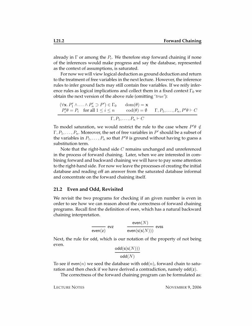
L21.2 Forward Chaining
already in Γ or among the Pi. We therefore stop forward chaining if noneof the inferences would make progress and say the database, representedas the context of assumptions, is saturated.
For now we will view logical deduction as ground deduction and returnto the treatment of free variables in the next lecture. However, the inferencerules to infer ground facts may still contain free variables. If we reify infer-ence rules as logical implications and collect them in a fixed context Γ0 weobtain the next version of the above rule (omitting ‘true’):
(∀x. P ′
1∧ . . . ∧ P ′
n⊃ P ′) ∈ Γ0
P ′
iθ = Pi for all 1 ≤ i ≤ n
dom(θ) = x
cod(θ) = ∅ Γ, P1, . . . , Pn, P ′θ ` C
Γ, P1, . . . , Pn ` C
To model saturation, we would restrict the rule to the case where P ′θ /∈
Γ, P1, . . . , Pn. Moreover, the set of free variables in P ′ should be a subset ofthe variables in P1, . . . , Pn so that P ′θ is ground without having to guess asubstitution term.
Note that the right-hand side C remains unchanged and unreferencedin the process of forward chaining. Later, when we are interested in com-bining forward and backward chaining we will have to pay some attentionto the right-hand side. For now we leave the processes of creating the initialdatabase and reading off an answer from the saturated database informaland concentrate on the forward chaining itself.
21.2 Even and Odd, Revisited
We revisit the two programs for checking if an given number is even inorder to see how we can reason about the correctness of forward chainingprograms. Recall first the definition of even, which has a natural backwardchaining interpretation.
even(z)evz
even(N)
even(s(s(N)))evss
Next, the rule for odd, which is our notation of the property of not beingeven.
odd(s(s(N)))
odd(N)
To see if even(n) we seed the database with odd(n), forward chain to satu-ration and then check if we have derived a contradiction, namely odd(z).
The correctness of the forward chaining program can be formulated as:
LECTURE NOTES NOVEMBER 9, 2006
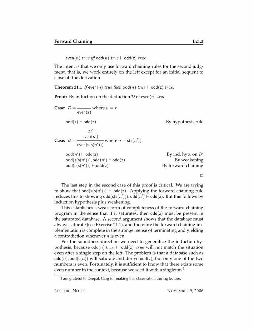
Forward Chaining L21.3
even(n) true iff odd(n) true ` odd(z) true
The intent is that we only use forward chaining rules for the second judg-ment, that is, we work entirely on the left except for an initial sequent toclose off the derivation.
Theorem 21.1 If even(n) true then odd(n) true ` odd(z) true .
Proof: By induction on the deduction D of even(n) true
Case: D =even(z)
where n = z.
odd(z) ` odd(z) By hypothesis rule
Case: D =
D′
even(n′)
even(s(s(n′)))where n = s(s(n′)).
odd(n′) ` odd(z) By ind. hyp. on D′
odd(s(s(n′))), odd(n′) ` odd(z) By weakeningodd(s(s(n′))) ` odd(z) By forward chaining
2
The last step in the second case of this proof is critical. We are tryingto show that odd(s(s(n′))) ` odd(z). Applying the forward chaining rulereduces this to showing odd(s(s(n′))), odd(n′) ` odd(z). But this follows byinduction hypothesis plus weakening.
This establishes a weak form of completeness of the forward chainingprogram in the sense that if it saturates, then odd(z) must be present inthe saturated database. A second argument shows that the database mustalways saturate (see Exercise 21.1), and therefore the forward chaining im-plementation is complete in the stronger sense of terminating and yieldinga contradiction whenever n is even.
For the soundness direction we need to generalize the induction hy-pothesis, because odd(n) true ` odd(z) true will not match the situationeven after a single step on the left. The problem is that a database such asodd(n), odd(s(n)) will saturate and derive odd(z), but only one of the twonumbers is even. Fortunately, it is sufficient to know that there exists someeven number in the context, because we seed it with a singleton.1
1I am grateful to Deepak Garg for making this observation during lecture.
LECTURE NOTES NOVEMBER 9, 2006
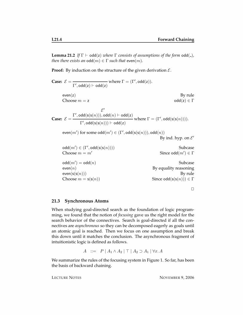
L21.4 Forward Chaining
Lemma 21.2 If Γ ` odd(z) where Γ consists of assumptions of the form odd( ),then there exists an odd(m) ∈ Γ such that even(m).
Proof: By induction on the structure of the given derivation E .
Case: E =Γ′, odd(z) ` odd(z)
where Γ = (Γ′, odd(z)).
even(z) By ruleChoose m = z odd(z) ∈ Γ
Case: E =
E ′
Γ′, odd(s(s(n))), odd(n) ` odd(z)
Γ′, odd(s(s(n))) ` odd(z)where Γ = (Γ′, odd(s(s(n)))).
even(m′) for some odd(m′) ∈ (Γ′, odd(s(s(n))), odd(n))By ind. hyp. on E ′
odd(m′) ∈ (Γ′, odd(s(s(n)))) SubcaseChoose m = m′ Since odd(m′) ∈ Γ
odd(m′) = odd(n) Subcaseeven(n) By equality reasoningeven(s(s(n))) By ruleChoose m = s(s(n)) Since odd(s(s(n))) ∈ Γ
2
21.3 Synchronous Atoms
When studying goal-directed search as the foundation of logic program-ming, we found that the notion of focusing gave us the right model for thesearch behavior of the connectives. Search is goal-directed if all the con-nectives are asynchronous so they can be decomposed eagerly as goals untilan atomic goal is reached. Then we focus on one assumption and breakthis down until it matches the conclusion. The asynchronous fragment ofintuitionistic logic is defined as follows.
A ::= P | A1 ∧ A2 | > | A2 ⊃ A1 | ∀x.A
We summarize the rules of the focusing system in Figure 1. So far, has beenthe basis of backward chaining.
LECTURE NOTES NOVEMBER 9, 2006

Forward Chaining L21.5
A ∈ Γ Γ;A � P
Γ ` PfocusL
Γ;P � PidR
no rule for P ′ 6= P
Γ;P ′ � P
Γ, A ` B
Γ ` A ⊃ B⊃R
Γ;B � P Γ ` A
Γ;A ⊃ B � P⊃L
Γ ` A Γ ` B
Γ ` A ∧ B∧R
Γ;A � P
Γ;A ∧ B � P∧L1
∆;B � P
Γ;A ∧ B � P∧L2
Γ ` >>R
no >L rule
Γ ` A x /∈ FV(Γ)
Γ ` ∀x.A∀R
∆;A(t/x) � P
Γ;∀x.A � P∀L
Figure 1: Focused Intuitionistic Logic; Asynchronous Fragment
Forward chaining violates the goal-directed nature of search, so weneed to depart from the purely asynchronous fragment. Our change is min-imalistic: we introduce only synchronous atomic propositions Q. For the sakeof economy we also interpret inference rules
C1 true . . . Cn true
Q true
without conjunction, writing them with iterated implication
∀x. C1 ⊃ (C2 ⊃ . . . (Cn ⊃ Q))
instead. Here, Ci are all atoms, be they asynchronous (P ) or synchronous(Q).
Since a goal can now be synchronous, we have the opportunity to focuson the right, if the right-hand side is a synchronous proposition (so far onlyQ). When a synchronous atomic proposition is in right focus, we succeedif the same proposition is in Γ; otherwise we fail.
Γ � Q
Γ ` QfocusR
Q ∈ Γ
Γ � QidL
no rule for Q /∈ ΓΓ � Q
LECTURE NOTES NOVEMBER 9, 2006
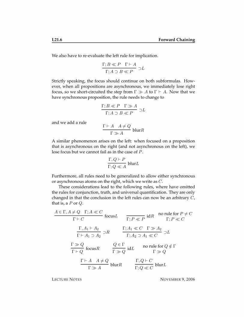
L21.6 Forward Chaining
We also have to re-evaluate the left rule for implication.
Γ;B � P Γ ` A
Γ;A ⊃ B � P⊃L
Strictly speaking, the focus should continue on both subformulas. How-ever, when all propositions are asynchronous, we immediately lose rightfocus, so we short-circuited the step from Γ � A to Γ ` A. Now that wehave synchronous proposition, the rule needs to change to
Γ;B � P Γ � A
Γ;A ⊃ B � P⊃L
and we add a ruleΓ ` A A 6= Q
Γ � AblurR
A similar phenomenon arises on the left: when focused on a propositionthat is asynchronous on the right (and not asynchronous on the left), welose focus but we cannot fail as in the case of P .
Γ, Q ` P
Γ;Q � AblurL
Furthermore, all rules need to be generalized to allow either synchronousor asynchronous atoms on the right, which we write as C .
These considerations lead to the following rules, where have omittedthe rules for conjunction, truth, and universal quantification. They are onlychanged in that the conclusion in the left rules can now be an arbitrary C ,that is, a P or Q.
A ∈ Γ, A 6= Q Γ;A � C
Γ ` CfocusL
Γ;P � PidR
no rule for P 6= C
Γ;P � C
Γ, A1 ` A2
Γ ` A1 ⊃ A2
⊃RΓ;A1 � C Γ � A2
Γ;A2 ⊃ A1 � C⊃L
Γ � Q
Γ ` QfocusR
Q ∈ Γ
Γ � QidL
no rule for Q /∈ ΓΓ � Q
Γ ` A A 6= Q
Γ � AblurR
Γ, Q ` C
Γ;Q � CblurL
LECTURE NOTES NOVEMBER 9, 2006
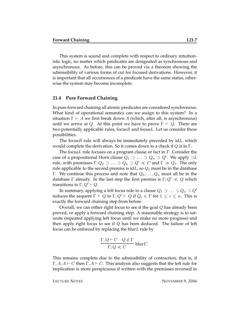
Forward Chaining L21.7
This system is sound and complete with respect to ordinary intuition-istic logic, no matter which predicates are designated as synchronous andasynchronous. As before, this can be proved via a theorem showing theadmissibility of various forms of cut for focused derivations. However, itis important that all occurrences of a predicate have the same status, other-wise the system may become incomplete.
21.4 Pure Forward Chaining
In pure forward chaining all atomic predicates are considered synchronous.What kind of operational semantics can we assign to this system? In asituation Γ ` A we first break down A (which, after all, is asynchronous)until we arrive at Q. At this point we have to prove Γ ` Q. There aretwo potentially applicable rules, focusR and focusL. Let us consider thesepossibilities.
The focusR rule will always be immediately preceded by idL, whichwould complete the derivation. So it comes down to a check if Q is in Γ.
The focusL rule focuses on a program clause or fact in Γ. Consider thecase of a propositional Horn clause Q1 ⊃ . . . ⊃ Qn ⊃ Q′. We apply ⊃L
rule, with premisses Γ;Q2 ⊃ . . . ⊃ Qn ⊃ Q′ � C and Γ � Q1. The onlyrule applicable to the second premiss is idL, so Q1 must be in the databaseΓ. We continue this process and note that Q2, . . . , Qn must all be in thedatabase Γ already. In the last step the first premiss is Γ;Q′ � Q whichtransitions to Γ, Q′ ` Q.
In summary, applying a left focus rule to a clause Q1 ⊃ . . . ⊃ Qn ⊃ Q′
reduces the sequent Γ ` Q to Γ, Q′ ` Q if Qi ∈ Γ for 1 ≤ i ≤ n. This isexactly the forward chaining step from before.
Overall, we can either right focus to see if the goal Q has already beenproved, or apply a forward chaining step. A reasonable strategy is to sat-urate (repeated applying left focus until we make no more progress) andthen apply right focus to see if Q has been deduced. The failure of leftfocus can be enforced by replacing the blurL rule by
Γ, Q ` C Q /∈ Γ
Γ;Q � CblurL′.
This remains complete due to the admissibility of contraction, that is, ifΓ, A,A ` C then Γ, A ` C . This analysis also suggests that the left rule forimplication is more perspicuous if written with the premisses reversed in
LECTURE NOTES NOVEMBER 9, 2006
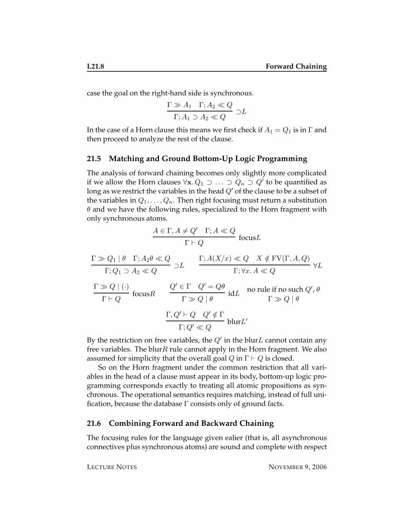
L21.8 Forward Chaining
case the goal on the right-hand side is synchronous.
Γ � A1 Γ;A2 � Q
Γ;A1 ⊃ A2 � Q⊃L
In the case of a Horn clause this means we first check if A1 = Q1 is in Γ andthen proceed to analyze the rest of the clause.
21.5 Matching and Ground Bottom-Up Logic Programming
The analysis of forward chaining becomes only slightly more complicatedif we allow the Horn clauses ∀x. Q1 ⊃ . . . ⊃ Qn ⊃ Q′ to be quantified aslong as we restrict the variables in the head Q′ of the clause to be a subset ofthe variables in Q1, . . . , Qn. Then right focusing must return a substitutionθ and we have the following rules, specialized to the Horn fragment withonly synchronous atoms.
A ∈ Γ, A 6= Q′ Γ;A � Q
Γ ` QfocusL
Γ � Q1 | θ Γ;A2θ � Q
Γ;Q1 ⊃ A2 � Q⊃L
Γ;A(X/x) � Q X /∈ FV(Γ, A,Q)
Γ;∀x.A � Q∀L
Γ � Q | (·)
Γ ` QfocusR
Q′ ∈ Γ Q′ = Qθ
Γ � Q | θidL
no rule if no such Q′, θ
Γ � Q | θ
Γ, Q′ ` Q Q′ /∈ Γ
Γ;Q′ � QblurL′
By the restriction on free variables, the Q′ in the blurL cannot contain anyfree variables. The blurR rule cannot apply in the Horn fragment. We alsoassumed for simplicity that the overall goal Q in Γ ` Q is closed.
So on the Horn fragment under the common restriction that all vari-ables in the head of a clause must appear in its body, bottom-up logic pro-gramming corresponds exactly to treating all atomic propositions as syn-chronous. The operational semantics requires matching, instead of full uni-fication, because the database Γ consists only of ground facts.
21.6 Combining Forward and Backward Chaining
The focusing rules for the language given ealier (that is, all asynchronousconnectives plus synchronous atoms) are sound and complete with respect
LECTURE NOTES NOVEMBER 9, 2006
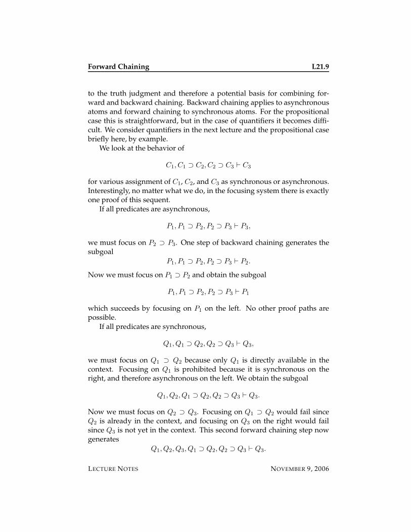
Forward Chaining L21.9
to the truth judgment and therefore a potential basis for combining for-ward and backward chaining. Backward chaining applies to asynchronousatoms and forward chaining to synchronous atoms. For the propositionalcase this is straightforward, but in the case of quantifiers it becomes diffi-cult. We consider quantifiers in the next lecture and the propositional casebriefly here, by example.
We look at the behavior of
C1, C1 ⊃ C2, C2 ⊃ C3 ` C3
for various assignment of C1, C2, and C3 as synchronous or asynchronous.Interestingly, no matter what we do, in the focusing system there is exactlyone proof of this sequent.
If all predicates are asynchronous,
P1, P1 ⊃ P2, P2 ⊃ P3 ` P3,
we must focus on P2 ⊃ P3. One step of backward chaining generates thesubgoal
P1, P1 ⊃ P2, P2 ⊃ P3 ` P2.
Now we must focus on P1 ⊃ P2 and obtain the subgoal
P1, P1 ⊃ P2, P2 ⊃ P3 ` P1
which succeeds by focusing on P1 on the left. No other proof paths arepossible.
If all predicates are synchronous,
Q1, Q1 ⊃ Q2, Q2 ⊃ Q3 ` Q3,
we must focus on Q1 ⊃ Q2 because only Q1 is directly available in thecontext. Focusing on Q1 is prohibited because it is synchronous on theright, and therefore asynchronous on the left. We obtain the subgoal
Q1, Q2, Q1 ⊃ Q2, Q2 ⊃ Q3 ` Q3.
Now we must focus on Q2 ⊃ Q3. Focusing on Q1 ⊃ Q2 would fail sinceQ2 is already in the context, and focusing on Q3 on the right would failsince Q3 is not yet in the context. This second forward chaining step nowgenerates
Q1, Q2, Q3, Q1 ⊃ Q2, Q2 ⊃ Q3 ` Q3.
LECTURE NOTES NOVEMBER 9, 2006
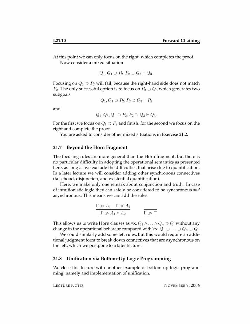
L21.10 Forward Chaining
At this point we can only focus on the right, which completes the proof.
Now consider a mixed situation
Q1, Q1 ⊃ P2, P2 ⊃ Q3 ` Q3.
Focusing on Q1 ⊃ P2 will fail, because the right-hand side does not matchP2. The only successful option is to focus on P2 ⊃ Q3 which generates twosubgoals
Q1, Q1 ⊃ P2, P2 ⊃ Q3 ` P2
and
Q1, Q3, Q1 ⊃ P2, P2 ⊃ Q3 ` Q3.
For the first we focus on Q1 ⊃ P2 and finish, for the second we focus on theright and complete the proof.
You are asked to consider other mixed situations in Exercise 21.2.
21.7 Beyond the Horn Fragment
The focusing rules are more general than the Horn fragment, but there isno particular difficulty in adopting the operational semantics as presentedhere, as long as we exclude the difficulties that arise due to quantification.In a later lecture we will consider adding other synchronous connectives(falsehood, disjunction, and existential quantification).
Here, we make only one remark about conjunction and truth. In caseof intuitionistic logic they can safely be considered to be synchronous andasynchronous. This means we can add the rules
Γ � A1 Γ � A2
Γ � A1 ∧ A2 Γ � >
This allows us to write Horn clauses as ∀x. Q1 ∧ . . . ∧Qn ⊃ Q′ without anychange in the operational behavior compared with ∀x. Q1 ⊃ . . . ⊃ Qn ⊃ Q′.
We could similarly add some left rules, but this would require an addi-tional judgment form to break down connectives that are asynchronous onthe left, which we postpone to a later lecture.
21.8 Unification via Bottom-Up Logic Programming
We close this lecture with another example of bottom-up logic program-ming, namely and implementation of unification.
LECTURE NOTES NOVEMBER 9, 2006
Forward Chaining L21.11
The implementation of unification by bottom-up logic programming il-lustrates a common type of program where saturation can be employedto great advantage. This is similar to the even example where we reasonby contradication for a decidable predicate. Here, the predicate is non-unifiability of two terms s and t, as well as non-unifiability of sequencesof terms s and t as an auxiliary predicate. In order to show that two termsare non-unifiable we assume they are unifiable, saturate, and then test theresulting saturated database for inconsistent information. We write s
.= t
and s.= t for the two equality relations.
Since there are a number of ways a contradiction can arise, we also in-troduce an explicit proposition contra to indicate a contradiction. In a laterlecture we will see that we can in fact use ⊥ with a sound logical interpre-tation, but that would requires us to go beyond the current setting.
The way to think about the rules is via the laws governing equality. Westart with symmetry, transitivity, and reflexivity. Reflexivity actually givesus no new information (we already know the two terms are equal), so thereis no forward rule for it.
s.= t
t.= s
s.= t t
.= r
s.= r
Not all instances of transitivity are actually required (see Exercise 21.3); re-stricting it can lead to an improvement in the running time of the algorithm.Next, the congruence rules for constructors and sequences.
f(s).= f(t)
s.= t
(s, s).= (t, t)
s.= t
(s, s).= (t, t)
s.= t
(·).= (·)
no rule
There is no rule for (·).= (·) since this fact does not yield any new infor-
mation. However, we have rules that note contradictory information byconcluding contra.
f(s).= g(t) f 6= g
contra
(·).= (t, t)
contra
(s, s).= (·)
contra
Even in the presence of variables, the rules so far will saturate, closing agiven equality under its consequences. We consider f(x, g(b))
.= f(a, g(x))
as an example and show the generated consequences, omitting any identi-
LECTURE NOTES NOVEMBER 9, 2006
L21.12 Forward Chaining
ties t.= t and intermediate steps relating a sequences to their elements.
f(x, g(b)).= f(a, g(x)) Assumption
f(a, g(x)).= f(x, g(b)) Symmetry
x.= a Congruence
g(b).= g(x) Congruence
a.= x Symmetry
g(x).= g(b) Symmetry
b.= x Congruence
x.= b Symmetry
b.= a Transitivity
a.= b Symmetry
contra Clash b 6= a
The only point missing from the overall strategy to is to generate a con-tradiction due to a failure of the occurs-check. For this we have two newforms of propositions, x /∈ t and x /∈ t which we use to propagate occur-rence information.
x.= f(t)
x /∈ t
x /∈ (t, t)
x /∈ t
x /∈ (t, t)
x /∈ t
x /∈ (·)
no rule
x /∈ f(t)
x /∈ t
x /∈ x
contra
x /∈ y, x 6= y
no rule
x /∈ t t.= s
x /∈ s
The last rule is necessary so that, for example, the set x.= f(y), y
.= f(x)
can be recognized as contradictory.
Let us apply the McAllester meta-complexity result. In the completeddatabase, any two subterms of the original unification problem may be setequal, so we have O(n2) possibilities. Transitivity has O(n3) prefix firings,so a cursory analysis yields O(n3) complexity. This is better than the ex-ponential complexity of Robinson’s algorithm, but still far worse then the
LECTURE NOTES NOVEMBER 9, 2006
Forward Chaining L21.13
linear time lower bound. Both the algorithm and the analysis can be re-fined in a number of ways. For example, we can restrict the uses of sym-metry and transitivity to obtain better bounds, and we can postpone theuse of non-occurrence to a second pass over a database saturated by theother rules.
This form of presentation of unification has become standard practice.It does not explicitly compute a unifier, but for unifiable terms it computesa kind of graph where the nodes in the original term (when viewed as adag) are the nodes, and nodes are related by explicit equalities. From this aunifier can be read off by looking up the equivalence classes of the variablesin the original unification problem.
Another nice property of unification, shared by many other saturation-based algorithms, is that it is incremental. This means that equations canbe added one by one, and the database saturated every time, starting fromthe previously saturated one. If the equations ever become contradictory,contra is derived.
Here is a sketch how this might be used in the implementation of a logicprogramming engine. We have a constraint store, initially empty. When-ever logic programming search would call unification to obtain a unifier,we instead assume the equation into the database and saturate it. If weobtain a contradiction, unification fails and we have to backtrack. If not,we continue with the resulting constraint store. A neat thing about this im-plementation is that we never explicitly need to compute and apply a mostgeneral unifier: any goal we consider is always with respect to a saturated(and therefore consistent) set of equations.
21.9 Historical Notes
Although the notion that atoms may be synchronous or asynchronous, atthe programmer’s discretion, is relatively old [1], I believe that the obser-vation connecting forward chaining to synchronous atoms is relatively re-cent [2], and was made in the setting of general theorem proving. An al-ternative approach to combining forward and backward chaining in logicprogramming using a monad [5] will be the subject of a later lecture.
The view of unification as a forward reasoning process similar to theone described here is due to Huet [3], although he maintained equivalenceclasses of terms much more efficiently than our naive specification, usingthe well-known union-find algorithm to arrive at an almost linear algo-rithm. Huet’s basic idea was later refined by Martelli and Montanari [6]and in a different way by Paterson and Wegman [7] to obtain linear time
LECTURE NOTES NOVEMBER 9, 2006
L21.14 Forward Chaining
algorithms for unification.The idea to handle unification problems via a store of constraints, to
be updated and queried during computation, goes back to constraint logicprogramming [4]. It was elevated to logical status by Saraswat [8], althoughthe connection to focusing, forward and backward chaining was not recog-nized at the time.
21.10 Exercises
Exercise 21.1 Prove that the database initialized with odd(n) for some n andclosed under forward application of the rule
odd(s(s(N)))
odd(N)
will always saturate in a finite number of steps.
Exercise 21.2 Consider two other ways to assign atoms to be synchronous orasynchronous for the sequent
C1, C1 ⊃ C2, C2 ⊃ C3 ` C3
from Section 21.6 and show that there exists a unique proof in each case.
Exercise 21.3 Improve the bottom-up unification algorithm by analyzing morecarefully which instances of symmetry and transitivity are really needed. You mayignore the occurs-check, which we assume could be done in a second pass after theother rules saturate. What kind of McAllester complexity does your analysis yield?
21.11 References
[1] Jean-Marc Andreoli. Logic programming with focusing proofs in linearlogic. Journal of Logic and Computation, 2(3):297–347, 1992.
[2] Kaustuv Chaudhuri, Frank Pfenning, and Greg Price. A logical charac-terization of forward and backward chaining in the inverse method. InU. Furbach and N. Shankar, editors, Proceedings of the 3rd InternationalJoint Conference on Automated Reasoning (IJCAR’06), pages 97–111, Seat-tle, Washington, August 2006. Springer LNCS 4130.
[3] Gerard Huet. Resolution d’equations dans des langages d’ordre 1, 2, . . . , ω.PhD thesis, Universite Paris VII, September 1976.
LECTURE NOTES NOVEMBER 9, 2006
Forward Chaining L21.15
[4] Joxan Jaffar and Jean-Louis Lassez. Constraint logic programming. InProceedings of the 14th Annual Symposium on Principles of ProgrammingLanguages, pages 111–119, Munich, Germany, January 1987. ACM Press.
[5] Pablo Lopez, Frank Pfenning, Jeff Polakow, and Kevin Watkins. Mon-adic concurrent linear logic programming. In A.Felty, editor, Proceed-ings of the 7th International Symposium on Principles and Practice of Declar-ative Programming (PPDP’05), pages 35–46, Lisbon, Portugal, July 2005.ACM Press.
[6] Alberto Martelli and Ugo Montanari. An efficient unification al-gorithm. ACM Transactions on Programming Languages and Systems,4(2):258–282, April 1982.
[7] M. S. Paterson and M. N. Wegman. Linear unification. Journal of Com-puter and System Sciences, 16(2):158–167, April 1978.
[8] Vijay Saraswat. Concurrent Constraint Programming. MIT Press, 1991.ACM Doctoral Dissertation Award Series.
LECTURE NOTES NOVEMBER 9, 2006

L21.16 Forward Chaining
LECTURE NOTES NOVEMBER 9, 2006
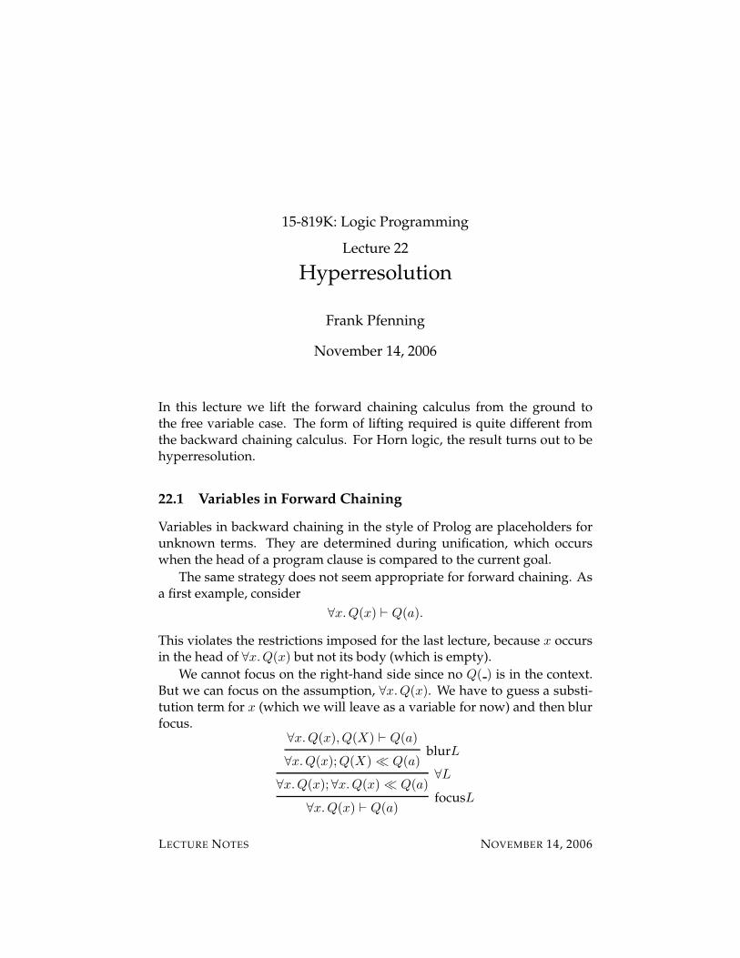
15-819K: Logic Programming
Lecture 22
Hyperresolution
Frank Pfenning
November 14, 2006
In this lecture we lift the forward chaining calculus from the ground tothe free variable case. The form of lifting required is quite different fromthe backward chaining calculus. For Horn logic, the result turns out to behyperresolution.
22.1 Variables in Forward Chaining
Variables in backward chaining in the style of Prolog are placeholders forunknown terms. They are determined during unification, which occurswhen the head of a program clause is compared to the current goal.
The same strategy does not seem appropriate for forward chaining. Asa first example, consider
∀x.Q(x) ` Q(a).
This violates the restrictions imposed for the last lecture, because x occursin the head of ∀x.Q(x) but not its body (which is empty).
We cannot focus on the right-hand side since no Q( ) is in the context.But we can focus on the assumption, ∀x.Q(x). We have to guess a substi-tution term for x (which we will leave as a variable for now) and then blurfocus.
∀x.Q(x), Q(X) ` Q(a)
∀x.Q(x);Q(X) � Q(a)blurL
∀x.Q(x);∀x.Q(x) � Q(a)∀L
∀x.Q(x) ` Q(a)focusL
LECTURE NOTES NOVEMBER 14, 2006
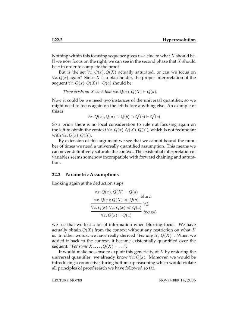
L22.2 Hyperresolution
Nothing within this focusing sequence gives us a clue to what X should be.If we now focus on the right, we can see in the second phase that X shouldbe a in order to complete the proof.
But is the set ∀x.Q(x), Q(X) actually saturated, or can we focus on∀x.Q(x) again? Since X is a placeholder, the proper interpretation of thesequent ∀x.Q(x), Q(X) ` Q(a) should be:
There exists an X such that ∀x.Q(x), Q(X) ` Q(a).
Now it could be we need two instances of the universal quantifier, so wemight need to focus again on the left before anything else. An example ofthis is
∀x.Q(x), Q(a) ⊃ Q(b) ⊃ Q′(c) ` Q′(c)
So a priori there is no local consideration to rule out focusing again onthe left to obtain the context ∀x.Q(x), Q(X), Q(Y ), which is not redundantwith ∀x.Q(x), Q(X).
By extension of this argument we see that we cannot bound the num-ber of times we need a universally quantified assumption. This means wecan never definitively saturate the context. The existential interpretation ofvariables seems somehow incompatible with forward chaining and satura-tion.
22.2 Parametric Assumptions
Looking again at the deduction steps
∀x.Q(x), Q(X) ` Q(a)
∀x.Q(x);Q(X) � Q(a)blurL
∀x.Q(x);∀x.Q(x) � Q(a)∀L
∀x.Q(x) ` Q(a)focusL
we see that we lost a lot of information when blurring focus. We haveactually obtain Q(X) from the context without any restriction on what X
is. In other words, we have really derived “For any X, Q(X)”. When weadded it back to the context, it became existentially quantified over thesequent: “For some X, . . . , Q(X) ` . . .”.
It would make no sense to exploit this genericity of X by restoring theuniversal quantifier: we already know ∀x.Q(x). Moreover, we would beintroducing a connective during bottom-up reasoning which would violateall principles of proof search we have followed so far.
LECTURE NOTES NOVEMBER 14, 2006
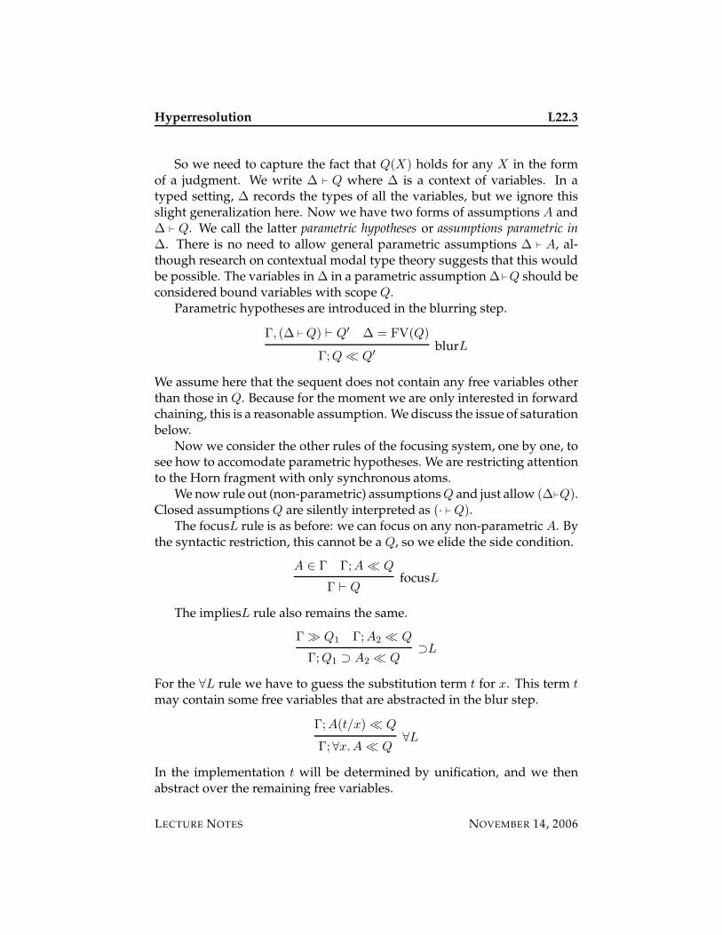
Hyperresolution L22.3
So we need to capture the fact that Q(X) holds for any X in the formof a judgment. We write ∆ ` Q where ∆ is a context of variables. In atyped setting, ∆ records the types of all the variables, but we ignore thisslight generalization here. Now we have two forms of assumptions A and∆ ` Q. We call the latter parametric hypotheses or assumptions parametric in∆. There is no need to allow general parametric assumptions ∆ ` A, al-though research on contextual modal type theory suggests that this wouldbe possible. The variables in ∆ in a parametric assumption ∆`Q should beconsidered bound variables with scope Q.
Parametric hypotheses are introduced in the blurring step.
Γ, (∆ ` Q) ` Q′ ∆ = FV(Q)
Γ;Q � Q′blurL
We assume here that the sequent does not contain any free variables otherthan those in Q. Because for the moment we are only interested in forwardchaining, this is a reasonable assumption. We discuss the issue of saturationbelow.
Now we consider the other rules of the focusing system, one by one, tosee how to accomodate parametric hypotheses. We are restricting attentionto the Horn fragment with only synchronous atoms.
We now rule out (non-parametric) assumptions Q and just allow (∆`Q).Closed assumptions Q are silently interpreted as (· ` Q).
The focusL rule is as before: we can focus on any non-parametric A. Bythe syntactic restriction, this cannot be a Q, so we elide the side condition.
A ∈ Γ Γ;A � Q
Γ ` QfocusL
The impliesL rule also remains the same.
Γ � Q1 Γ;A2 � Q
Γ;Q1 ⊃ A2 � Q⊃L
For the ∀L rule we have to guess the substitution term t for x. This term t
may contain some free variables that are abstracted in the blur step.
Γ;A(t/x) � Q
Γ;∀x.A � Q∀L
In the implementation t will be determined by unification, and we thenabstract over the remaining free variables.
LECTURE NOTES NOVEMBER 14, 2006
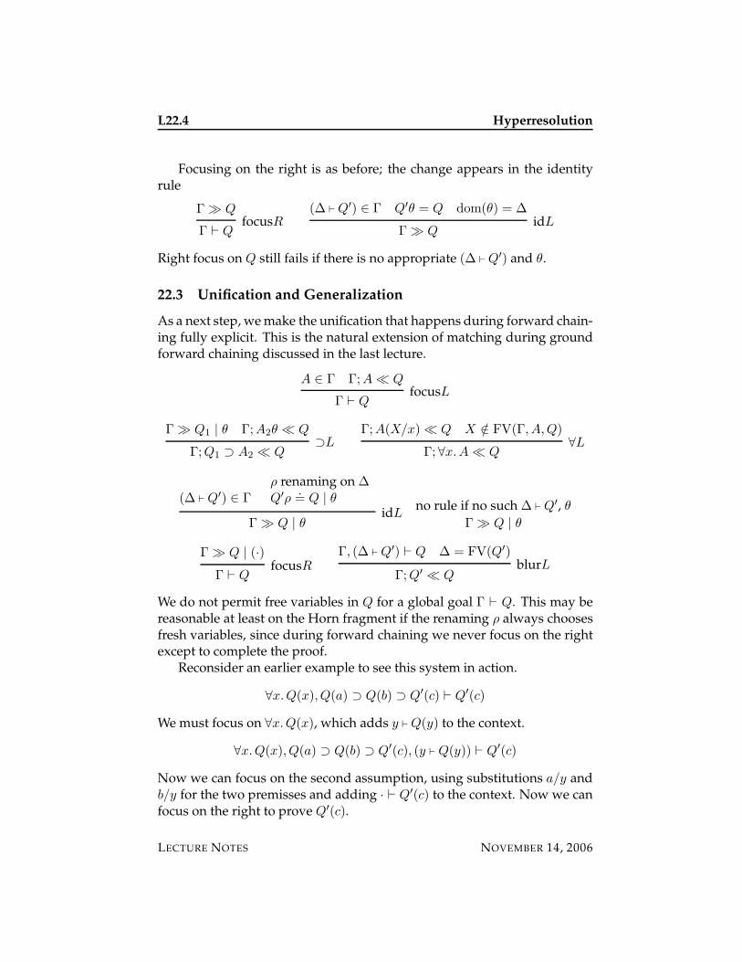
L22.4 Hyperresolution
Focusing on the right is as before; the change appears in the identityrule
Γ � Q
Γ ` QfocusR
(∆ ` Q′) ∈ Γ Q′θ = Q dom(θ) = ∆
Γ � QidL
Right focus on Q still fails if there is no appropriate (∆ ` Q′) and θ.
22.3 Unification and Generalization
As a next step, we make the unification that happens during forward chain-ing fully explicit. This is the natural extension of matching during groundforward chaining discussed in the last lecture.
A ∈ Γ Γ;A � Q
Γ ` QfocusL
Γ � Q1 | θ Γ;A2θ � Q
Γ;Q1 ⊃ A2 � Q⊃L
Γ;A(X/x) � Q X /∈ FV(Γ, A,Q)
Γ;∀x.A � Q∀L
(∆ ` Q′) ∈ Γρ renaming on ∆Q′ρ
.= Q | θ
Γ � Q | θidL
no rule if no such ∆ ` Q′, θ
Γ � Q | θ
Γ � Q | (·)
Γ ` QfocusR
Γ, (∆ ` Q′) ` Q ∆ = FV(Q′)
Γ;Q′ � QblurL
We do not permit free variables in Q for a global goal Γ ` Q. This may bereasonable at least on the Horn fragment if the renaming ρ always choosesfresh variables, since during forward chaining we never focus on the rightexcept to complete the proof.
Reconsider an earlier example to see this system in action.
∀x.Q(x), Q(a) ⊃ Q(b) ⊃ Q′(c) ` Q′(c)
We must focus on ∀x.Q(x), which adds y ` Q(y) to the context.
∀x.Q(x), Q(a) ⊃ Q(b) ⊃ Q′(c), (y ` Q(y)) ` Q′(c)
Now we can focus on the second assumption, using substitutions a/y andb/y for the two premisses and adding · ` Q′(c) to the context. Now we canfocus on the right to prove Q′(c).
LECTURE NOTES NOVEMBER 14, 2006
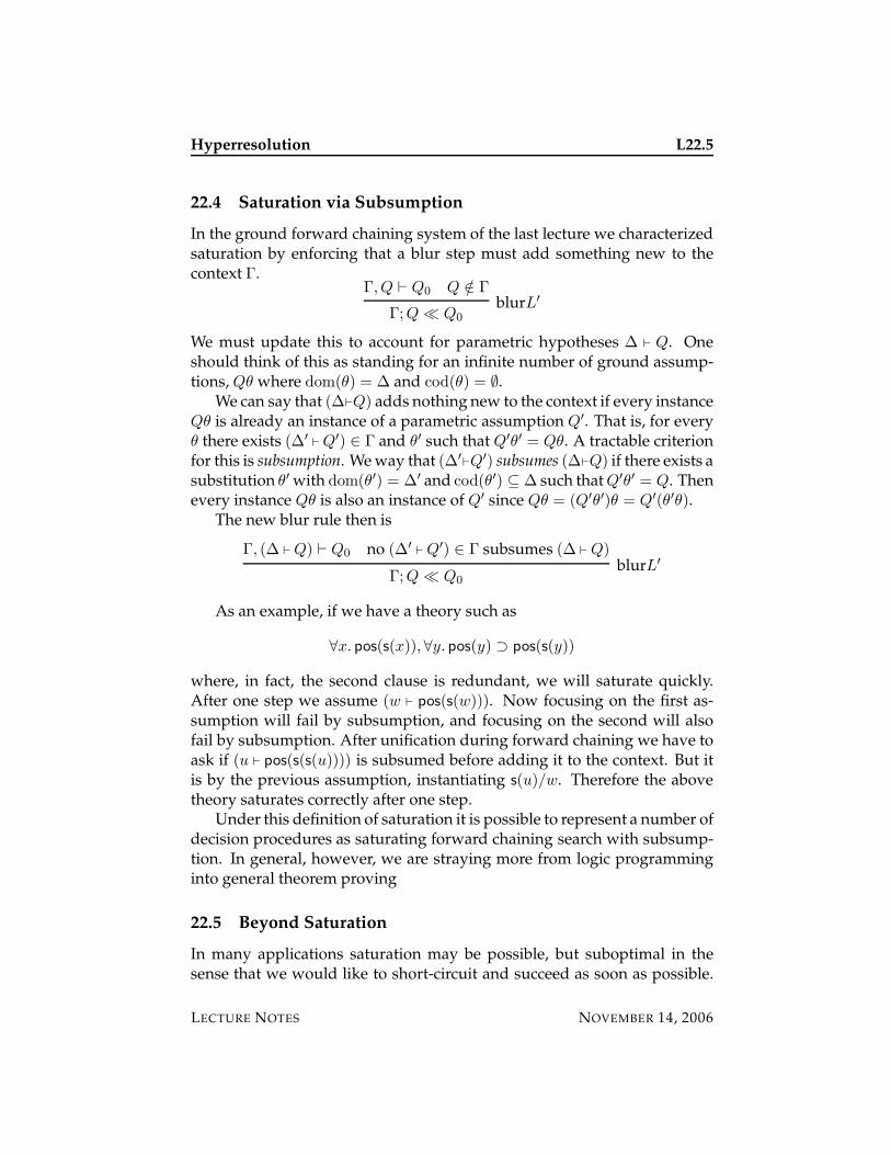
Hyperresolution L22.5
22.4 Saturation via Subsumption
In the ground forward chaining system of the last lecture we characterizedsaturation by enforcing that a blur step must add something new to thecontext Γ.
Γ, Q ` Q0 Q /∈ Γ
Γ;Q � Q0
blurL′
We must update this to account for parametric hypotheses ∆ ` Q. Oneshould think of this as standing for an infinite number of ground assump-tions, Qθ where dom(θ) = ∆ and cod(θ) = ∅.
We can say that (∆`Q) adds nothing new to the context if every instanceQθ is already an instance of a parametric assumption Q′. That is, for everyθ there exists (∆′
` Q′) ∈ Γ and θ′ such that Q′θ′ = Qθ. A tractable criterionfor this is subsumption. We way that (∆′
`Q′) subsumes (∆`Q) if there exists asubstitution θ′ with dom(θ′) = ∆′ and cod(θ′) ⊆ ∆ such that Q′θ′ = Q. Thenevery instance Qθ is also an instance of Q′ since Qθ = (Q′θ′)θ = Q′(θ′θ).
The new blur rule then is
Γ, (∆ ` Q) ` Q0 no (∆′` Q′) ∈ Γ subsumes (∆ ` Q)
Γ;Q � Q0
blurL′
As an example, if we have a theory such as
∀x. pos(s(x)),∀y. pos(y) ⊃ pos(s(y))
where, in fact, the second clause is redundant, we will saturate quickly.After one step we assume (w ` pos(s(w))). Now focusing on the first as-sumption will fail by subsumption, and focusing on the second will alsofail by subsumption. After unification during forward chaining we have toask if (u ` pos(s(s(u)))) is subsumed before adding it to the context. But itis by the previous assumption, instantiating s(u)/w. Therefore the abovetheory saturates correctly after one step.
Under this definition of saturation it is possible to represent a number ofdecision procedures as saturating forward chaining search with subsump-tion. In general, however, we are straying more from logic programminginto general theorem proving
22.5 Beyond Saturation
In many applications saturation may be possible, but suboptimal in thesense that we would like to short-circuit and succeed as soon as possible.
LECTURE NOTES NOVEMBER 14, 2006
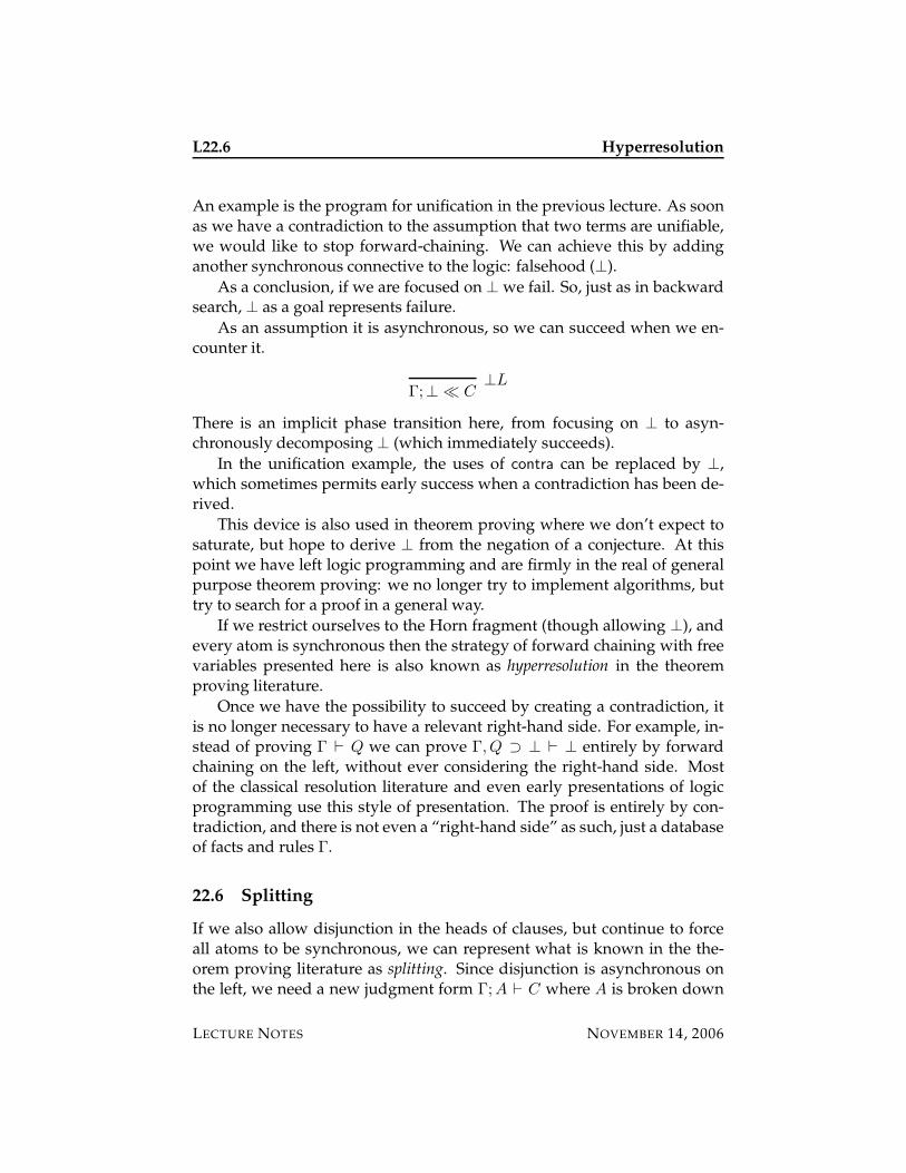
L22.6 Hyperresolution
An example is the program for unification in the previous lecture. As soonas we have a contradiction to the assumption that two terms are unifiable,we would like to stop forward-chaining. We can achieve this by addinganother synchronous connective to the logic: falsehood (⊥).
As a conclusion, if we are focused on ⊥ we fail. So, just as in backwardsearch, ⊥ as a goal represents failure.
As an assumption it is asynchronous, so we can succeed when we en-counter it.
Γ;⊥ � C⊥L
There is an implicit phase transition here, from focusing on ⊥ to asyn-chronously decomposing ⊥ (which immediately succeeds).
In the unification example, the uses of contra can be replaced by ⊥,which sometimes permits early success when a contradiction has been de-rived.
This device is also used in theorem proving where we don’t expect tosaturate, but hope to derive ⊥ from the negation of a conjecture. At thispoint we have left logic programming and are firmly in the real of generalpurpose theorem proving: we no longer try to implement algorithms, buttry to search for a proof in a general way.
If we restrict ourselves to the Horn fragment (though allowing ⊥), andevery atom is synchronous then the strategy of forward chaining with freevariables presented here is also known as hyperresolution in the theoremproving literature.
Once we have the possibility to succeed by creating a contradiction, itis no longer necessary to have a relevant right-hand side. For example, in-stead of proving Γ ` Q we can prove Γ, Q ⊃ ⊥ ` ⊥ entirely by forwardchaining on the left, without ever considering the right-hand side. Mostof the classical resolution literature and even early presentations of logicprogramming use this style of presentation. The proof is entirely by con-tradiction, and there is not even a “right-hand side” as such, just a databaseof facts and rules Γ.
22.6 Splitting
If we also allow disjunction in the heads of clauses, but continue to forceall atoms to be synchronous, we can represent what is known in the the-orem proving literature as splitting. Since disjunction is asynchronous onthe left, we need a new judgment form Γ;A ` C where A is broken down
LECTURE NOTES NOVEMBER 14, 2006
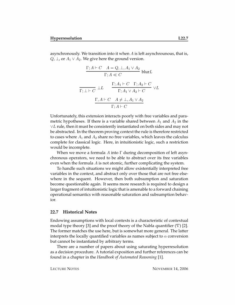
Hyperresolution L22.7
asynchronously. We transition into it when A is left asynchrounous, that is,Q, ⊥, or A1 ∨ A2. We give here the ground version.
Γ;A ` C A = Q,⊥, A1 ∨ A2
Γ;A � CblurL
Γ;⊥ ` C⊥L
Γ;A1 ` C Γ;A2 ` C
Γ;A1 ∨ A2 ` C∨L
Γ, A ` C A 6= ⊥, A1 ∨ A2
Γ;A ` C
Unfortunately, this extension interacts poorly with free variables and para-metric hypotheses. If there is a variable shared between A1 and A2 in the∨L rule, then it must be consistently instantiated on both sides and may notbe abstracted. In the theorem proving context the rule is therefore restrictedto cases where A1 and A2 share no free variables, which leaves the calculuscomplete for classical logic. Here, in intuitionistic logic, such a restrictionwould be incomplete.
When we move a formula A into Γ during decomposition of left asyn-chronous operators, we need to be able to abstract over its free variableseven when the formula A is not atomic, further complicating the system.
To handle such situations we might allow existentially interpreted freevariables in the context, and abstract only over those that are not free else-where in the sequent. However, then both subsumption and saturationbecome questionable again. It seems more research is required to design alarger fragment of intuitionistic logic that is amenable to a forward chainingoperational semantics with reasonable saturation and subsumption behav-ior.
22.7 Historical Notes
Endowing assumptions with local contexts is a characteristic of contextualmodal type theory [3] and the proof theory of the Nabla quantifier (∇) [2].The former matches the use here, but is somewhat more general. The latterinterprets the locally quantified variables as names subject to α conversionbut cannot be instantiated by arbitrary terms.
There are a number of papers about using saturating hyperresolutionas a decision procedure. A tutorial exposition and further references can befound in a chapter in the Handbook of Automated Reasoning [1].
LECTURE NOTES NOVEMBER 14, 2006
L22.8 Hyperresolution
22.8 References
[1] Christian Fermuller, Alexander Leitsch, Ullrich Hustadt, and TanelTammet. Resolution decision procedures. In Alan Robinson and An-drei Voronkov, editors, Handbook of Automated Reasoning, volume 2,chapter 25, pages 1791–1849. Elsevier Science and MIT Press, 2001.
[2] Dale Miller and Alwen Tiu. A proof theory for generic judgments.ACM Transactions on Computational Logic, 6(4):749–783, October 2005.
[3] Aleksandar Nanevski, Frank Pfenning, and Brigitte Pientka. Contex-tual modal type theory. Submitted, September 2005.
LECTURE NOTES NOVEMBER 14, 2006
15-819K: Logic Programming
Lecture 23
Linear Monadic Logic Programming
Frank Pfenning
November 16, 2006
In this lecture we extend the observations about forward and backwardchaining from Horn logic to a rich set of linear connectives. In order tocontrol the interaction between forward and backward chaining we use amonad to separate asynchronous from synchronous connectives. The re-sult is the logic programming language LolliMon, which we illustrate withsome examples.
23.1 Separating Asynchronous and Synchronous Connectives
The observations we have made about focusing, forward chaining, andbackward chaining apply to various logics, including linear logic, whichwas indeed the origin of the notion of focusing. But it is difficult to com-bine forward and backward chaining and obtain a satisfactory operationalsemantics.
The problem can be broadly described as follows. First, if all connec-tives are asynchronous we obtain a clear and non-deterministically com-plete backward chaining semantics. Second, on the Horn fragment withonly synchronous atoms we obtain a satisfactory forward chaining seman-tics with saturation. However, adding more synchronous connectives, ormixing synchronous with asynchronous connectives introduces a lot of un-controlled non-determinism into the operational reading of programs. Weapproach general theorem proving, leaving the predictable operational be-havior of Prolog behind.
We do not rule out that it may be possible to obtain a satisfactory se-mantics, but in this lecture we pursue a different path. We can controlthe interaction between asynchronous and synchronous connectives and
LECTURE NOTES NOVEMBER 16, 2006
L23.2 Linear Monadic Logic Programming
therefore between backward and forward chaining by creating a firewallbetween them called a monad. From the logical point of view a monad is aso-called lax modal operator. We will explain its laws below. For now we justnote that we write {−} for the modal operator.
In a complex linear logic proposition we can identify the places wherewe change from asynchronous to synchronous connectives or vice versa.At the first transition we require the explicit monadic firewall; the secondtransition is simply an inclusion. There is one exception, namely in a linearimplication we switch sides (if the implication appears on the right the an-tecedent appears on the left), so we have to switch from asynchronous tosynchronous propositions to remain in the same phase of decomposition.
Asynch A ::= P | A1 & A2 | > | S1 ( A2 | A1 ⊃ A2 | ∀x.A | {S}
Synch S ::= Q | S1 ⊕ S2 | 0 | S1 ⊗ S2 | 1 | !A | ∃x. S | A
Recall that P stands for asynchronous atoms and Q for synchronousatoms. We observe that the exponential modality of linear logic, !, has a spe-cial status: !A is synchronous but the subformula does not continue the syn-chronous phase, but is asynchronous. Similarly, A1 ⊃ A2 is asynchronous,but A1 in the antecedent which we might expect to be synchronous is infact asynchronous. We will briefly explain this phenomenon later in thelecture.
We have been inclusive here, omitting only S1 ⊗! A2 and s.= t which
were necessary for residuation. The first is easy to add or define. Explicitequality is omitted here because in this lecture we concentrate on proposi-tional and modal aspects of computation (see Exercise 23.2).
23.2 The Lax Modality
In order for the lax modality to have the right effect in separating the for-ward and backward chaining phases, we need to give it a proper logicalfoundation. In this section we just present this logical meaning; later wejustify its role in the operational semantics. Since the semantics here is fullygeneral, and does not depend on the division into asynchronous and syn-chronous operators, we just use B and C to stand for arbitrary propositionin linear logic, augmented by the lax modality.
In addition to the usual judgment B true we have a new judgment onpropositions, B lax . This can given be many different readings. Let us thinkof it for now as “B is true subject to some (abstract) constraint”. This means
LECTURE NOTES NOVEMBER 16, 2006

Linear Monadic Logic Programming L23.3
that B lax is a weaker judgment then B true .
∆ ` B true
∆ ` B laxlax
This is a rule concerned only with the judgment, not with the propositionwhich remains unchanged. Of course, this rule is not invertible, or truthand lax truth would coincide. As in the prior sections on linear logic weomit the unrestricted context from the rules since it is generally just propa-gated from conclusion to premisses.
The second property is a form of the cut principle: if we can derive B lax
we are allowed to assume B true , but only if we are deriving a lax conclu-sion. This is so because deriving a lax conclusion permits a constraint.
If ∆B ` B lax and ∆C , B true ` C lax then ∆C ,∆B ` C lax .
This should always hold, which means it is admissible when formulatedas a rule of inference. This is not the case if we changed the conclusion toC true since then we could derive the converse of the first rule, and truthand lax truth collapse.
The right and left rules for the lax modality are now straightforward.
∆ ` B lax
∆ ` {B} true{−}R
∆, B true ` C lax
∆, {B} true ` C lax{−}L
Again, the conclusion of the {−}L rule is restricted to the form C lax ; al-lowing C true here would be incorrect.
However, the other left rules in the sequent calculus must now per-mit an arbitrary judgment J on the right-hand side, which could be eitherC true or C lax where previously in could only be C true . The prior proofof the admissibility of cut and the identity principle can be easily extendedto this fragment.
In terms of focusing, the modal operator looks at first a bit odd. In adeduction (read bottom-up), we go from {B} true to B lax and from thereto B true .
On the right, the first transition is asynchronous: we can always stripthe modal operator. The second transition is synchronous: we may have towait for a left rule to be applied (specifically: to go from {C} true to C true
for some C) before we can prove B true.On the left, the first transition is synchronous: we cannot remove the
modal operator until the right-hand side has the form C lax . The second
LECTURE NOTES NOVEMBER 16, 2006
L23.4 Linear Monadic Logic Programming
one, however, is asynchronous, because B true is a stronger assumptionthan B lax .
We can also see this from the proof of the identity principle.
B true ` B true
B true ` B laxlax
{B} true ` B lax{−}L
{B} true ` {B} true{−}R
There is a “silent” transition on the left-hand side from B lax to B true . Be-cause the lax judgment is asynchronous as an assumption, we never needto consider it on the left-hand side.
23.3 The Exponential Modality Revisited
Above we have seen that the lax modality internalizes the judgment of laxtruth, which is weaker than truth. Conversely, the exponential modality!B of linear logic internalizes necessary truth (written B valid ), which isstronger than truth. Recall first the judgmental rule, given here with a moregeneral right hand-side J which could be C true or C lax .
Γ, B valid ;∆, B true ` J
Γ, B valid ;∆ ` Jcopy
The cut-like principle encodes that B is valid if it is true, without using anyany truth assumptions.
If Γ; · ` B true and Γ, B valid ;∆ ` J then Γ;∆ ` J .
When we internalize validity as a modal connective we obtain the follow-ing right and left rules.
Γ; · ` B true
Γ; · ` !B true!R
Γ, B valid ;∆ ` J
Γ;∆, !B true ` J!L
We see that the left rule expresses that if !B true then B valid . On theright-hand side, however, we have a silent transition from !B true , throughB valid to B true .
From this we can easily derive the focusing behavior. !B is synchronouson the right, but the judgment B valid is asynchronous. We therefore neverneed to explicitly consider B valid as a conclusion.
LECTURE NOTES NOVEMBER 16, 2006
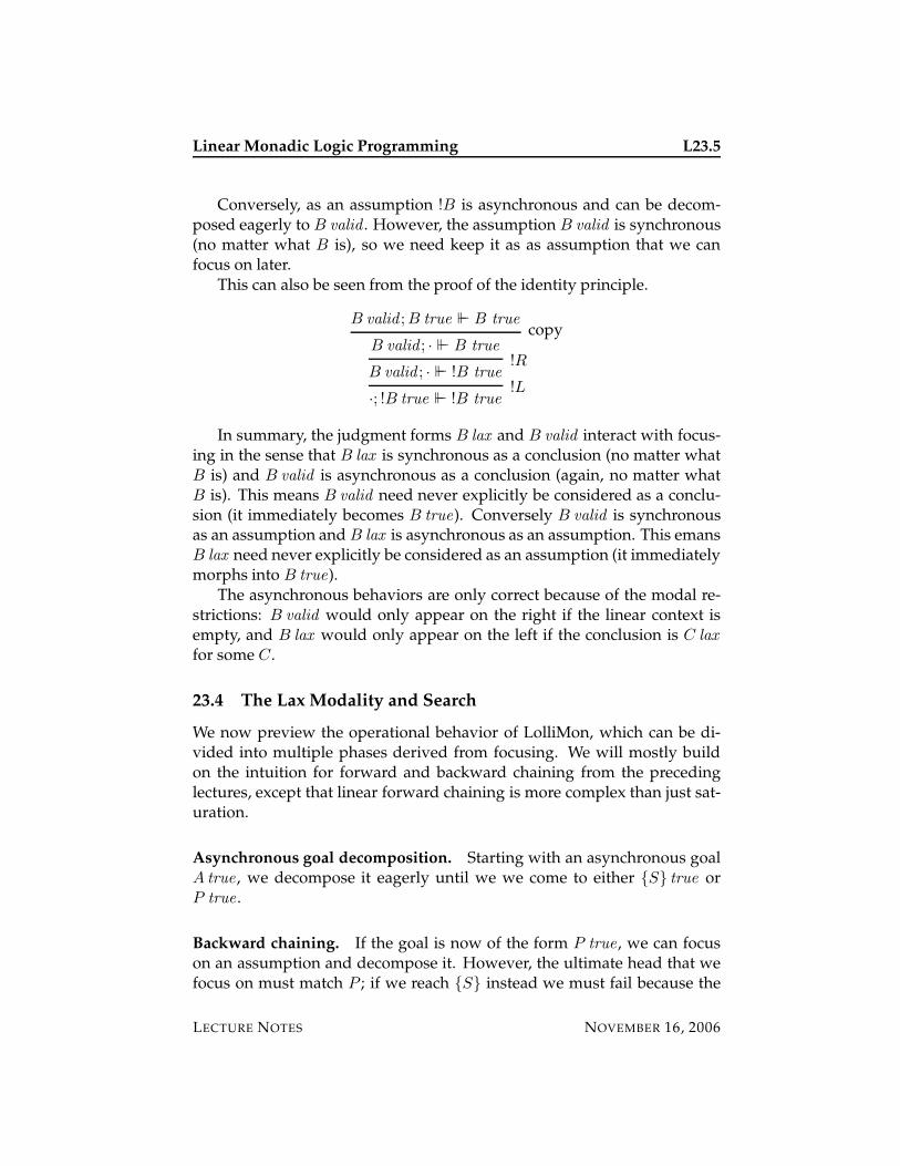
Linear Monadic Logic Programming L23.5
Conversely, as an assumption !B is asynchronous and can be decom-posed eagerly to B valid . However, the assumption B valid is synchronous(no matter what B is), so we need keep it as as assumption that we canfocus on later.
This can also be seen from the proof of the identity principle.
B valid ;B true ` B true
B valid ; · ` B truecopy
B valid ; · ` !B true!R
·; !B true ` !B true!L
In summary, the judgment forms B lax and B valid interact with focus-ing in the sense that B lax is synchronous as a conclusion (no matter whatB is) and B valid is asynchronous as a conclusion (again, no matter whatB is). This means B valid need never explicitly be considered as a conclu-sion (it immediately becomes B true). Conversely B valid is synchronousas an assumption and B lax is asynchronous as an assumption. This emansB lax need never explicitly be considered as an assumption (it immediatelymorphs into B true).
The asynchronous behaviors are only correct because of the modal re-strictions: B valid would only appear on the right if the linear context isempty, and B lax would only appear on the left if the conclusion is C lax
for some C .
23.4 The Lax Modality and Search
We now preview the operational behavior of LolliMon, which can be di-vided into multiple phases derived from focusing. We will mostly buildon the intuition for forward and backward chaining from the precedinglectures, except that linear forward chaining is more complex than just sat-uration.
Asynchronous goal decomposition. Starting with an asynchronous goalA true , we decompose it eagerly until we we come to either {S} true orP true .
Backward chaining. If the goal is now of the form P true , we can focuson an assumption and decompose it. However, the ultimate head that wefocus on must match P ; if we reach {S} instead we must fail because the
LECTURE NOTES NOVEMBER 16, 2006
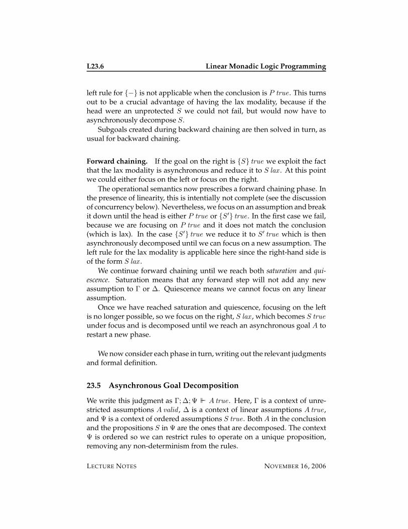
L23.6 Linear Monadic Logic Programming
left rule for {−} is not applicable when the conclusion is P true . This turnsout to be a crucial advantage of having the lax modality, because if thehead were an unprotected S we could not fail, but would now have toasynchronously decompose S.
Subgoals created during backward chaining are then solved in turn, asusual for backward chaining.
Forward chaining. If the goal on the right is {S} true we exploit the factthat the lax modality is asynchronous and reduce it to S lax . At this pointwe could either focus on the left or focus on the right.
The operational semantics now prescribes a forward chaining phase. Inthe presence of linearity, this is intentially not complete (see the discussionof concurrency below). Nevertheless, we focus on an assumption and breakit down until the head is either P true or {S′} true . In the first case we fail,because we are focusing on P true and it does not match the conclusion(which is lax). In the case {S′} true we reduce it to S′ true which is thenasynchronously decomposed until we can focus on a new assumption. Theleft rule for the lax modality is applicable here since the right-hand side isof the form S lax .
We continue forward chaining until we reach both saturation and qui-escence. Saturation means that any forward step will not add any newassumption to Γ or ∆. Quiescence means we cannot focus on any linearassumption.
Once we have reached saturation and quiescence, focusing on the leftis no longer possible, so we focus on the right, S lax , which becomes S true
under focus and is decomposed until we reach an asynchronous goal A torestart a new phase.
We now consider each phase in turn, writing out the relevant judgmentsand formal definition.
23.5 Asynchronous Goal Decomposition
We write this judgment as Γ;∆;Ψ ` A true . Here, Γ is a context of unre-stricted assumptions A valid , ∆ is a context of linear assumptions A true ,and Ψ is a context of ordered assumptions S true . Both A in the conclusionand the propositions S in Ψ are the ones that are decomposed. The contextΨ is ordered so we can restrict rules to operate on a unique proposition,removing any non-determinism from the rules.
LECTURE NOTES NOVEMBER 16, 2006
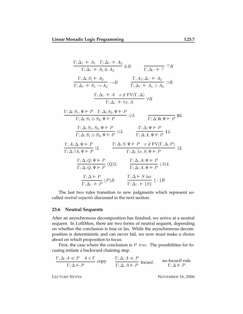
Linear Monadic Logic Programming L23.7
Γ;∆; · ` A1 Γ;∆; · ` A2
Γ;∆; · ` A1 & A2
&RΓ;∆; · ` >
>R
Γ;∆;S1 ` A2
Γ;∆; · ` S1 ( A2
(RΓ, A1;∆; · ` A2
Γ;∆; · ` A1 ⊃ A2
⊃R
Γ;∆; · ` A x /∈ FV(Γ,∆)
Γ;∆; · ` ∀x.A∀R
Γ;∆;S1,Ψ ` P Γ;∆;S2,Ψ ` P
Γ;∆;S1 ⊕ S2,Ψ ` P⊕L
Γ;∆;0,Ψ ` P0L
Γ;∆;S1, S2,Ψ ` P
Γ;∆;S1 ⊗ S2,Ψ ` P⊗L
Γ;∆;Ψ ` P
Γ;∆;1,Ψ ` P1L
Γ, A;∆;Ψ ` P
Γ;∆; !A,Ψ ` P!L
Γ;∆;S,Ψ ` P x /∈ FV(Γ,∆, P )
Γ;∆;∃x. S,Ψ ` P∃L
Γ;∆, Q; Ψ ` P
Γ;∆;Q,Ψ ` P(Q)L
Γ;∆, A; Ψ ` P
Γ;∆;A,Ψ ` P(A)L
Γ;∆ ` P
Γ;∆; · ` P(P )R
Γ;∆ ` S lax
Γ;∆; · ` {S}{−}R
The last two rules transition to new judgments which represent so-called neutral sequents discussed in the next section.
23.6 Neutral Sequents
After an asynchronous decomposition has finished, we arrive at a neutralsequent. In LolliMon, there are two forms of neutral sequent, dependingon whether the conclusion is true or lax. While the asynchronous decom-position is deterministic and can never fail, we now must make a choiceabout on which proposition to focus.
First, the case where the conclusion is P true . The possibilities for fo-cusing initiate a backward chaining step.
Γ;∆;A � P A ∈ Γ
Γ;∆ ` Pcopy
Γ;∆;A � P
Γ;∆, A ` PfocusL no focusR rule
Γ;∆ ` P
LECTURE NOTES NOVEMBER 16, 2006
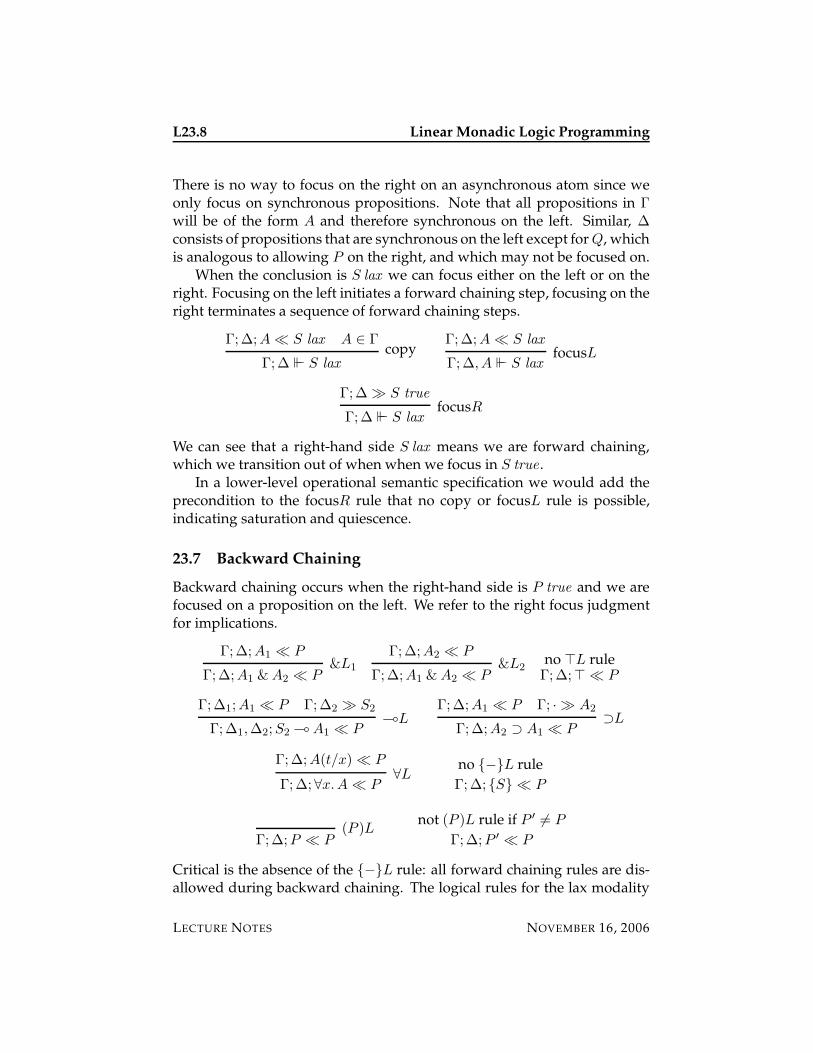
L23.8 Linear Monadic Logic Programming
There is no way to focus on the right on an asynchronous atom since weonly focus on synchronous propositions. Note that all propositions in Γwill be of the form A and therefore synchronous on the left. Similar, ∆consists of propositions that are synchronous on the left except for Q, whichis analogous to allowing P on the right, and which may not be focused on.
When the conclusion is S lax we can focus either on the left or on theright. Focusing on the left initiates a forward chaining step, focusing on theright terminates a sequence of forward chaining steps.
Γ;∆;A � S lax A ∈ Γ
Γ;∆ ` S laxcopy
Γ;∆;A � S lax
Γ;∆, A ` S laxfocusL
Γ;∆ � S true
Γ;∆ ` S laxfocusR
We can see that a right-hand side S lax means we are forward chaining,which we transition out of when when we focus in S true .
In a lower-level operational semantic specification we would add theprecondition to the focusR rule that no copy or focusL rule is possible,indicating saturation and quiescence.
23.7 Backward Chaining
Backward chaining occurs when the right-hand side is P true and we arefocused on a proposition on the left. We refer to the right focus judgmentfor implications.
Γ;∆;A1 � P
Γ;∆;A1 & A2 � P&L1
Γ;∆;A2 � P
Γ;∆;A1 & A2 � P&L2
no >L ruleΓ;∆;> � P
Γ;∆1;A1 � P Γ;∆2 � S2
Γ;∆1,∆2;S2 ( A1 � P(L
Γ;∆;A1 � P Γ; · � A2
Γ;∆;A2 ⊃ A1 � P⊃L
Γ;∆;A(t/x) � P
Γ;∆;∀x.A � P∀L
no {−}L rule
Γ;∆; {S} � P
Γ;∆;P � P(P )L
not (P )L rule if P ′ 6= P
Γ;∆;P ′ � P
Critical is the absence of the {−}L rule: all forward chaining rules are dis-allowed during backward chaining. The logical rules for the lax modality
LECTURE NOTES NOVEMBER 16, 2006
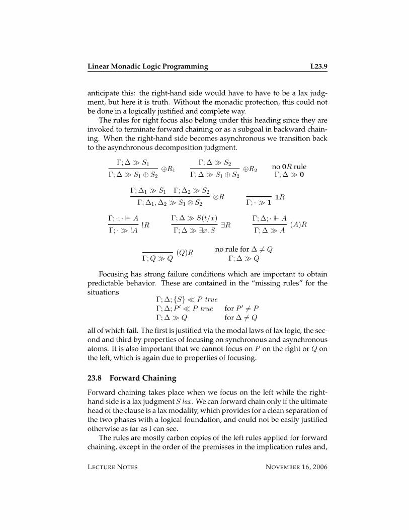
Linear Monadic Logic Programming L23.9
anticipate this: the right-hand side would have to have to be a lax judg-ment, but here it is truth. Without the monadic protection, this could notbe done in a logically justified and complete way.
The rules for right focus also belong under this heading since they areinvoked to terminate forward chaining or as a subgoal in backward chain-ing. When the right-hand side becomes asynchronous we transition backto the asynchronous decomposition judgment.
Γ;∆ � S1
Γ;∆ � S1 ⊕ S2
⊕R1
Γ;∆ � S2
Γ;∆ � S1 ⊕ S2
⊕R2no 0R ruleΓ;∆ � 0
Γ;∆1 � S1 Γ;∆2 � S2
Γ;∆1,∆2 � S1 ⊗ S2
⊗RΓ; · � 1
1R
Γ; ·; · ` A
Γ; · � !A!R
Γ;∆ � S(t/x)
Γ;∆ � ∃x. S∃R
Γ;∆; · ` A
Γ;∆ � A(A)R
Γ;Q � Q(Q)R no rule for ∆ 6= Q
Γ;∆ � Q
Focusing has strong failure conditions which are important to obtainpredictable behavior. These are contained in the “missing rules” for thesituations
Γ;∆; {S} � P true
Γ;∆;P ′ � P true for P ′ 6= P
Γ;∆ � Q for ∆ 6= Q
all of which fail. The first is justified via the modal laws of lax logic, the sec-ond and third by properties of focusing on synchronous and asynchronousatoms. It is also important that we cannot focus on P on the right or Q onthe left, which is again due to properties of focusing.
23.8 Forward Chaining
Forward chaining takes place when we focus on the left while the right-hand side is a lax judgment S lax . We can forward chain only if the ultimatehead of the clause is a lax modality, which provides for a clean separation ofthe two phases with a logical foundation, and could not be easily justifiedotherwise as far as I can see.
The rules are mostly carbon copies of the left rules applied for forwardchaining, except in the order of the premisses in the implication rules and,
LECTURE NOTES NOVEMBER 16, 2006
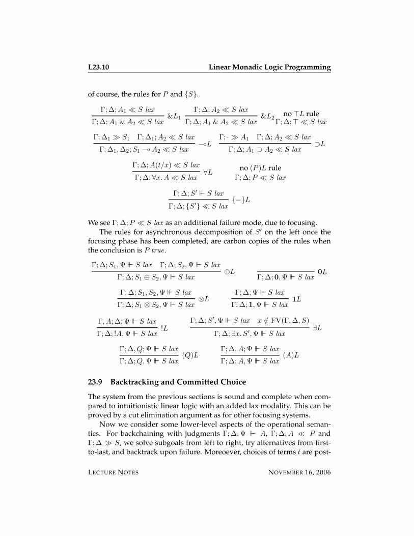
L23.10 Linear Monadic Logic Programming
of course, the rules for P and {S}.
Γ;∆;A1 � S lax
Γ;∆;A1 & A2 � S lax&L1
Γ;∆;A2 � S lax
Γ;∆;A1 & A2 � S lax&L2
no >L ruleΓ;∆;> � S lax
Γ;∆1 � S1 Γ;∆1;A2 � S lax
Γ;∆1,∆2;S1 ( A2 � S lax(L
Γ; · � A1 Γ;∆;A2 � S lax
Γ;∆;A1 ⊃ A2 � S lax⊃L
Γ;∆;A(t/x) � S lax
Γ;∆;∀x.A � S lax∀L
no (P )L rule
Γ;∆;P � S lax
Γ;∆;S′ ` S lax
Γ;∆; {S′} � S lax{−}L
We see Γ;∆;P � S lax as an additional failure mode, due to focusing.The rules for asynchronous decomposition of S′ on the left once the
focusing phase has been completed, are carbon copies of the rules whenthe conclusion is P true .
Γ;∆;S1,Ψ ` S lax Γ;∆;S2,Ψ ` S lax
Γ;∆;S1 ⊕ S2,Ψ ` S lax⊕L
Γ;∆;0,Ψ ` S lax0L
Γ;∆;S1, S2,Ψ ` S lax
Γ;∆;S1 ⊗ S2,Ψ ` S lax⊗L
Γ;∆;Ψ ` S lax
Γ;∆;1,Ψ ` S lax1L
Γ, A;∆;Ψ ` S lax
Γ;∆; !A,Ψ ` S lax!L
Γ;∆;S′,Ψ ` S lax x /∈ FV(Γ,∆, S)
Γ;∆;∃x. S′,Ψ ` S lax∃L
Γ;∆, Q; Ψ ` S lax
Γ;∆;Q,Ψ ` S lax(Q)L
Γ;∆, A; Ψ ` S lax
Γ;∆;A,Ψ ` S lax(A)L
23.9 Backtracking and Committed Choice
The system from the previous sections is sound and complete when com-pared to intuitionistic linear logic with an added lax modality. This can beproved by a cut elimination argument as for other focusing systems.
Now we consider some lower-level aspects of the operational seman-tics. For backchaining with judgments Γ;∆;Ψ ` A, Γ;∆;A � P andΓ;∆ � S, we solve subgoals from left to right, try alternatives from first-to-last, and backtrack upon failure. Moreoever, choices of terms t are post-
LECTURE NOTES NOVEMBER 16, 2006
Linear Monadic Logic Programming L23.11
poned and determined by unification. So the backchaining fragment of Lol-liMon is fully consistent with pure Prolog and Lolli, that is, logic program-ming in the asynchronous fragment of linear logic. It is weakly completewhich means that failure implies that a proof does not exist, but not all truepropositions can be proven due to potentially non-terminating depth-firstsearch.
For forward chaining, as defined by the judgments Γ;∆;A � S lax andΓ;∆;S′ ` S lax we use committed choice selection of the assumption to fo-cus on. Moreoever, we continue to forward chain until we reach saturationand quiescence before we focus on the lax goal on the right. At present,we would consider it an error if we encounter a free logic variable duringforward chaining because the semantics of this has not been satisfactorilysettled.
If the program does not use the linear context in an essential way (thatis, we are simulating unrestricted forward chaining in the linear setting),then due to the monotonicity of the unrestricted assumptions we still havenon-deterministic completeness.
If the program does use the linear context then the system is complete inonly a very weak sense: if we can always happen to make the right choicewe can find a proof if it exists, but even if computation fails a proof mightstill exist because we do not backtrack.
I believe that this is actually the desired behavior because linear for-ward chaining was designed to model concurrency. The operational se-mantics of forward chaining corresponds exactly to the operational seman-tics of concurrent languages such as CCS or the π-calculus: if a transitionis possible it may be taken without any chance for backtracking over thischoice. This means programs are correct only if all legal computations be-have correctly, such as, for example, avoiding deadlock. A correspondingcorrectness criteria applies to LolliMon program that use linear forwardchaining: we must write the program in such a way that if multiple choicescan be made, each one will give a correct answer in the end. The examplein the next section illustrates this point.
As a programming language the logical fragment we have identifiedhere is quite rich, since it allows backward chaining, saturating forwardchaining, and linear forward chaining to capture many different sorts ofoperational behavior. We have to guard against viewing it as a general pur-pose inference engine. For example, it is often easy to write down a con-current system as a linear LolliMon specification, but LolliMon presentlyprovides little help in analyzing such a specification beyond simulating in-dividual runs. This is an interesting area of further research.
LECTURE NOTES NOVEMBER 16, 2006
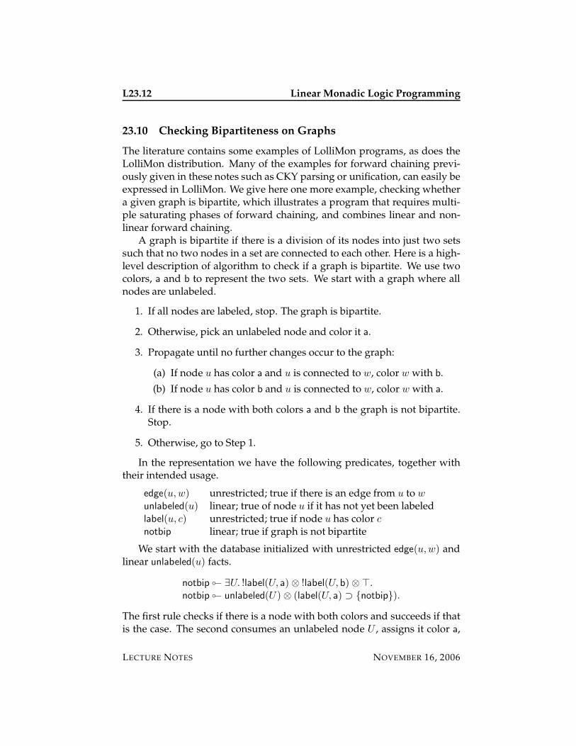
L23.12 Linear Monadic Logic Programming
23.10 Checking Bipartiteness on Graphs
The literature contains some examples of LolliMon programs, as does theLolliMon distribution. Many of the examples for forward chaining previ-ously given in these notes such as CKY parsing or unification, can easily beexpressed in LolliMon. We give here one more example, checking whethera given graph is bipartite, which illustrates a program that requires multi-ple saturating phases of forward chaining, and combines linear and non-linear forward chaining.
A graph is bipartite if there is a division of its nodes into just two setssuch that no two nodes in a set are connected to each other. Here is a high-level description of algorithm to check if a graph is bipartite. We use twocolors, a and b to represent the two sets. We start with a graph where allnodes are unlabeled.
1. If all nodes are labeled, stop. The graph is bipartite.
2. Otherwise, pick an unlabeled node and color it a.
3. Propagate until no further changes occur to the graph:
(a) If node u has color a and u is connected to w, color w with b.
(b) If node u has color b and u is connected to w, color w with a.
4. If there is a node with both colors a and b the graph is not bipartite.Stop.
5. Otherwise, go to Step 1.
In the representation we have the following predicates, together withtheir intended usage.
edge(u,w) unrestricted; true if there is an edge from u to w
unlabeled(u) linear; true of node u if it has not yet been labeledlabel(u, c) unrestricted; true if node u has color c
notbip linear; true if graph is not bipartite
We start with the database initialized with unrestricted edge(u,w) andlinear unlabeled(u) facts.
notbip ◦− ∃U. !label(U, a) ⊗ !label(U, b) ⊗>.
notbip ◦− unlabeled(U) ⊗ (label(U, a) ⊃ {notbip}).
The first rule checks if there is a node with both colors and succeeds if thatis the case. The second consumes an unlabeled node U , assigns it color a,
LECTURE NOTES NOVEMBER 16, 2006

Linear Monadic Logic Programming L23.13
saturates by forward chaining, and then recurses, starting the next itera-tion of the algorithm. notbip fails if there is no two-colored node and nounlabeled node, in which case the graph is indeed bipartite.
The first two forward chaining rules are straightforward.
!label(U, a) ⊗ !edge(U,W ) ( {!label(U, b)}.!label(U, b) ⊗ !edge(U,W ) ( {!label(U, a)}.
The third rule contains the interaction between linear and unrestricted as-sumptions: if a previously unlabeled node has been labeled, remove theassumption that it is unlabeled.
!label(U,C) ⊗ unlabeled(U) ( {1}.
Finally, a rule to take the symmetric closure of the edge relation, needed ifwe do not want to assume the relation is symmetric to start with.
!edge(U,W ) ( {!edge(W,U)}.
Syntactically, edge(u,w), label(u, c), and notbip must be asynchronousatoms. Atoms unlabeled(u) could be either synchronous or asynchronous,and both posibilities execute correctly. A synchronous interpretation ismost natural. There is a version of this program where label is also linear, inwhich case it would also be most naturally interpreted synchronously (seeExercise 23.4).
23.11 Historical Notes
The presentation of the lax modality in the form presented here originateswith [3]; see that paper for further references on modal logic and monads.
LolliMon1 [2] is a relatively recent development. The language sup-ported by the implementation and described in the paper is slightly differ-ent from what we discussed here. In particular, all atoms are asynchronous,and nested implications in forward chaining are processed in reverse or-der to what we show here. Moreover, the implementation does not fullysupport ⊕ and 0, but its term language is a simply-typed λ-calculus withprefix polymorphism solved by pattern unification. One aspect of this isdiscussed in the next lecture.
An example applying LolliMon in computer security is given by Po-lakow and Skalka [4].
1Distribution available at http://www.cs.cmu.edu/~fp/lollimon/
LECTURE NOTES NOVEMBER 16, 2006
L23.14 Linear Monadic Logic Programming
LolliMon originated in the work on the Concurrent Logical Framework(CLF) [6, 1]. CLF is a type theory for formalizing deductive systems sup-porting state (through linearity) and concurrency (through a lax modality).Its original formulation lacks disjunction (⊕) and falsehood (0), but per-mits dependent types and a rich term language. The most recent and mostcomplete work on the foundation of CLF is by Watkins [5].
23.12 Exercises
Exercise 23.1 Extend the LolliMon language from this lecture, adding equalitys
.= t and S ⊗! A, both of which are synchronous as goals and asynchronous as
assumptions.
Exercise 23.2 Some compound connectives in LolliMon are redundant and couldbe eliminated. For example, A1 ⊃ A2 is equivalently expressed by (!A1) ( A2.Consider which connectives are redundant in this sense in the language.
Exercise 23.3 We have hinted in a prior lecture on resource management that,though logically equivalent, certain connectives may still be important for opera-tional reasons. For example, S ⊗! A and S ⊗ (!A) have different resource manage-ment behavior. Reconsider the redundant operators you identified in response tothe Exercise 23.2 and determine which ones also have identical resource manage-ment properties and which do not.
Exercise 23.4 Rewrite the program to check whether graphs are bipartite, makingthe label predicate linear.
On this program, consider the assignment where both unlabeled and label aresynchronous and the one where both are asynchronous. Explain differences inoperational behavior, if any. Discuss which is more natural or potentially moreefficient.
23.13 References
[1] Iliano Cervesato, Frank Pfenning, David Walker, and Kevin Watkins. Aconcurrent logical framework II: Examples and applications. TechnicalReport CMU-CS-02-102, Department of Computer Science, CarnegieMellon University, 2002. Revised May 2003.
[2] Pablo Lopez, Frank Pfenning, Jeff Polakow, and Kevin Watkins. Mon-adic concurrent linear logic programming. In A.Felty, editor, Proceed-ings of the 7th International Symposium on Principles and Practice of Declar-
LECTURE NOTES NOVEMBER 16, 2006
Linear Monadic Logic Programming L23.15
ative Programming (PPDP’05), pages 35–46, Lisbon, Portugal, July 2005.ACM Press.
[3] Frank Pfenning and Rowan Davies. A judgmental reconstruction ofmodal logic. Mathematical Structures in Computer Science, 11:511–540,2001. Notes to an invited talk at the Workshop on Intuitionistic ModalLogics and Applications (IMLA’99), Trento, Italy, July 1999.
[4] Jeff Polakow and Christian Skalka. Specifying distributed trust man-agement in LolliMon. In S.Zdancewic and V.R.Sreedhar, editors, Pro-ceedings of the Workshop on Programming Languages and Security, Ottawa,Canada, June 2006. ACM.
[5] Kevin Watkins. CLF: A logical framework for concurrent systems. The-sis Proposal, May 2003.
[6] Kevin Watkins, Iliano Cervesato, Frank Pfenning, and David Walker. Aconcurrent logical framework I: Judgments and properties. TechnicalReport CMU-CS-02-101, Department of Computer Science, CarnegieMellon University, 2002. Revised May 2003.
LECTURE NOTES NOVEMBER 16, 2006
L23.16 Linear Monadic Logic Programming
LECTURE NOTES NOVEMBER 16, 2006
15-819K: Logic Programming
Lecture 24
Metavariables
Frank Pfenning
November 28, 2006
In this lecture we return to the treatment of logic variables. In Prolog andsome extensions we have considered, logic variables are global, and equa-tions involving logic variables are solved by unification. However, whenuniversal goals ∀x.A are allowed in backward chaining, or existential as-sumptions ∃x.A in forward chaining, new parameters may be introducedinto the proof search process. Ordinary unification on logic variables isnow unsound, even with the occurs-check. We generalize logic variablesto metavariables, a terminology borrowed from proof assistants and logicalframeworks, and describe unification in this extended setting.
24.1 Parameters
When proving a universally quantified proposition we demand that proofto be parametric. In the rule this is enforced by requiring that x be new.
Γ;∆ ` A x /∈ FV(Γ,∆)
Γ;∆ ` ∀x.A∀R
The condition on x can always be satisfied by renaming the bound vari-able. Operationally, this means that we introduce a new parameter into thederivation when solving a goal ∀x.A.
We already exploited the parametricity of the derivation for the admis-sibility of cut by substituting a term t for x in the subderivation. The ad-missibility of cut, rewritten here for lax linear logic, has the following form,with J standing for either C true or C lax :
IfD
Γ;∆D ` A andE
Γ;∆E , A ` J thenF
Γ;∆E ,∆D ` J .
LECTURE NOTES NOVEMBER 28, 2006
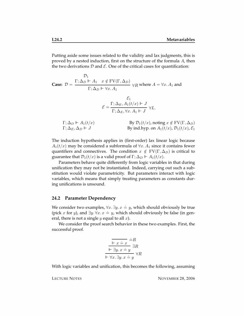
L24.2 Metavariables
Putting aside some issues related to the validity and lax judgments, this isproved by a nested induction, first on the structure of the formula A, thenthe two derivations D and E . One of the critical cases for quantification:
Case: D =
D1
Γ;∆D ` A1 x /∈ FV(Γ,∆D)
Γ;∆D ` ∀x.A1
∀R where A = ∀x.A1 and
E =
E1
Γ;∆E , A1(t/x) ` J
Γ;∆E ,∀x.A1 ` J∀L.
Γ;∆D ` A1(t/x) By D1(t/x), noting x /∈ FV(Γ,∆D)Γ;∆E,∆D ` J By ind.hyp. on A1(t/x), D1(t/x), E1
The induction hypothesis applies in (first-order) lax linear logic becauseA1(t/x) may be considered a subformula of ∀x.A1 since it contains fewerquantifiers and connectives. The condition x /∈ FV(Γ,∆D) is critical toguarantee that D1(t/x) is a valid proof of Γ;∆D ` A1(t/x).
Parameters behave quite differently from logic variables in that duringunification they may not be instantiated. Indeed, carrying out such a sub-stitution would violate parametricity. But parameters interact with logicvariables, which means that simply treating parameters as constants dur-ing unifications is unsound.
24.2 Parameter Dependency
We consider two examples, ∀x.∃y. x.= y, which should obviously be true
(pick x for y), and ∃y.∀x. x.= y, which should obviously be false (in gen-
eral, there is not a single y equal to all x).
We consider the proof search behavior in these two examples. First, thesuccessful proof.
` x.= x
.=R
` ∃y. x.= y
∃R
` ∀x.∃y. x.= y
∀R
With logic variables and unification, this becomes the following, assuming
LECTURE NOTES NOVEMBER 28, 2006
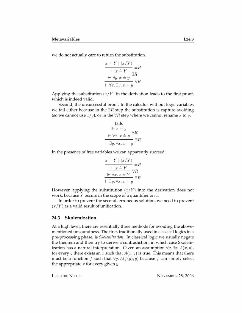
Metavariables L24.3
we do not actually care to return the substitution.
x.= Y | (x/Y )
` x.= Y
.=R
` ∃y. x.= y
∃R
` ∀x.∃y. x.= y
∀R
Applying the substitution (x/Y ) in the derivation leads to the first proof,which is indeed valid.
Second, the unsuccessful proof. In the calculus without logic variableswe fail either because in the ∃R step the substitution is capture-avoiding(so we cannot use x/y), or in the ∀R step where we cannot rename x to y.
fails` x
.= y
` ∀x. x.= y
∀R
` ∃y.∀x. x.= y
∃R
In the presence of free variables we can apparently succeed:
x.= Y | (x/Y )
` x.= Y
.=R
` ∀x. x.= Y
∀R
` ∃y.∀x. x.= y
∃R
However, applying the substitution (x/Y ) into the derivation does notwork, because Y occurs in the scope of a quantifier on x.
In order to prevent the second, erroneous solution, we need to prevent(x/Y ) as a valid result of unification.
24.3 Skolemization
At a high level, there are essentially three methods for avoiding the above-mentioned unsoundness. The first, traditionally used in classical logics in apre-processing phase, is Skolemization. In classical logic we usually negatethe theorem and then try to derive a contradiction, in which case Skolem-ization has a natural interpretation. Given an assumption ∀y.∃x.A(x, y),for every y there exists an x such that A(x, y) is true. This means that theremust be a function f such that ∀y.A(f(y), y) because f can simply selectthe appropriate x for every given y.
LECTURE NOTES NOVEMBER 28, 2006
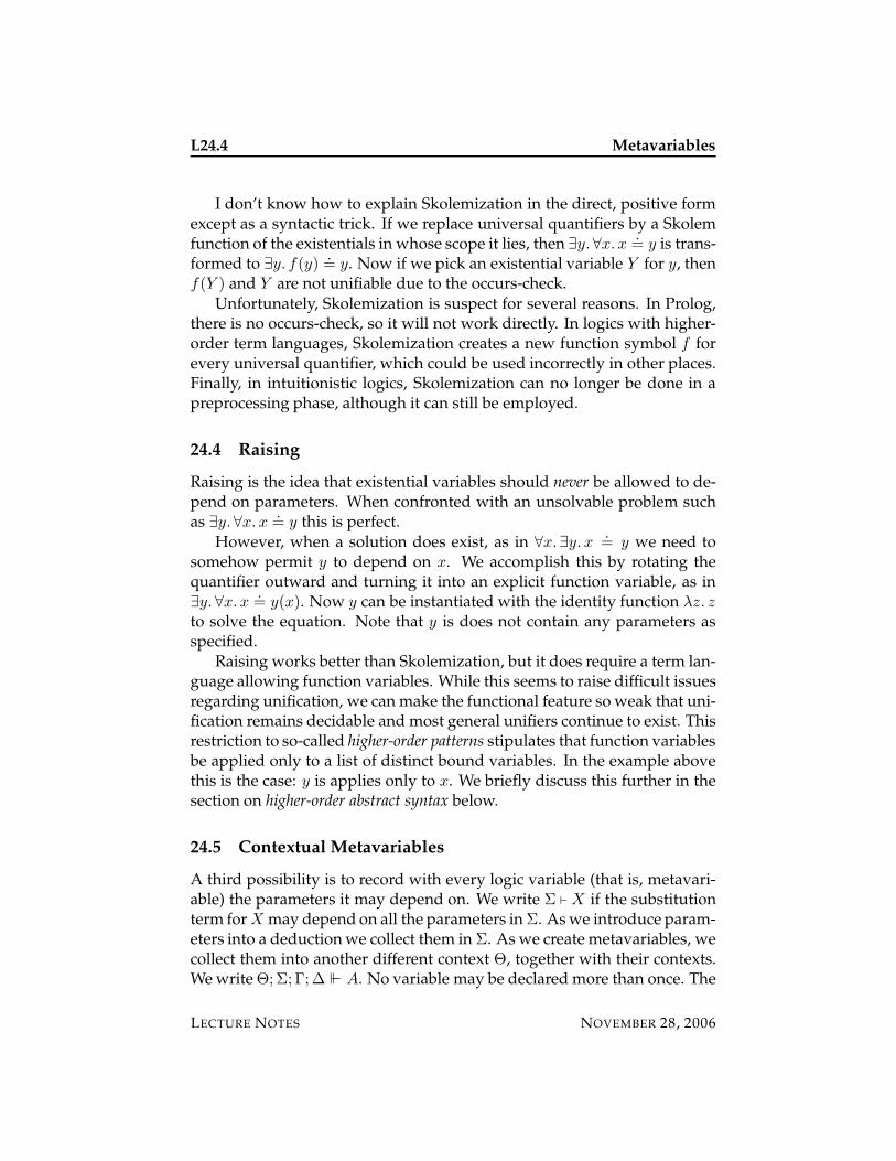
L24.4 Metavariables
I don’t know how to explain Skolemization in the direct, positive formexcept as a syntactic trick. If we replace universal quantifiers by a Skolemfunction of the existentials in whose scope it lies, then ∃y.∀x. x
.= y is trans-
formed to ∃y. f(y).= y. Now if we pick an existential variable Y for y, then
f(Y ) and Y are not unifiable due to the occurs-check.
Unfortunately, Skolemization is suspect for several reasons. In Prolog,there is no occurs-check, so it will not work directly. In logics with higher-order term languages, Skolemization creates a new function symbol f forevery universal quantifier, which could be used incorrectly in other places.Finally, in intuitionistic logics, Skolemization can no longer be done in apreprocessing phase, although it can still be employed.
24.4 Raising
Raising is the idea that existential variables should never be allowed to de-pend on parameters. When confronted with an unsolvable problem suchas ∃y.∀x. x
.= y this is perfect.
However, when a solution does exist, as in ∀x.∃y. x.= y we need to
somehow permit y to depend on x. We accomplish this by rotating thequantifier outward and turning it into an explicit function variable, as in∃y.∀x. x
.= y(x). Now y can be instantiated with the identity function λz. z
to solve the equation. Note that y is does not contain any parameters asspecified.
Raising works better than Skolemization, but it does require a term lan-guage allowing function variables. While this seems to raise difficult issuesregarding unification, we can make the functional feature so weak that uni-fication remains decidable and most general unifiers continue to exist. Thisrestriction to so-called higher-order patterns stipulates that function variablesbe applied only to a list of distinct bound variables. In the example abovethis is the case: y is applies only to x. We briefly discuss this further in thesection on higher-order abstract syntax below.
24.5 Contextual Metavariables
A third possibility is to record with every logic variable (that is, metavari-able) the parameters it may depend on. We write Σ ` X if the substitutionterm for X may depend on all the parameters in Σ. As we introduce param-eters into a deduction we collect them in Σ. As we create metavariables, wecollect them into another different context Θ, together with their contexts.We write Θ;Σ; Γ;∆ ` A. No variable may be declared more than once. The
LECTURE NOTES NOVEMBER 28, 2006
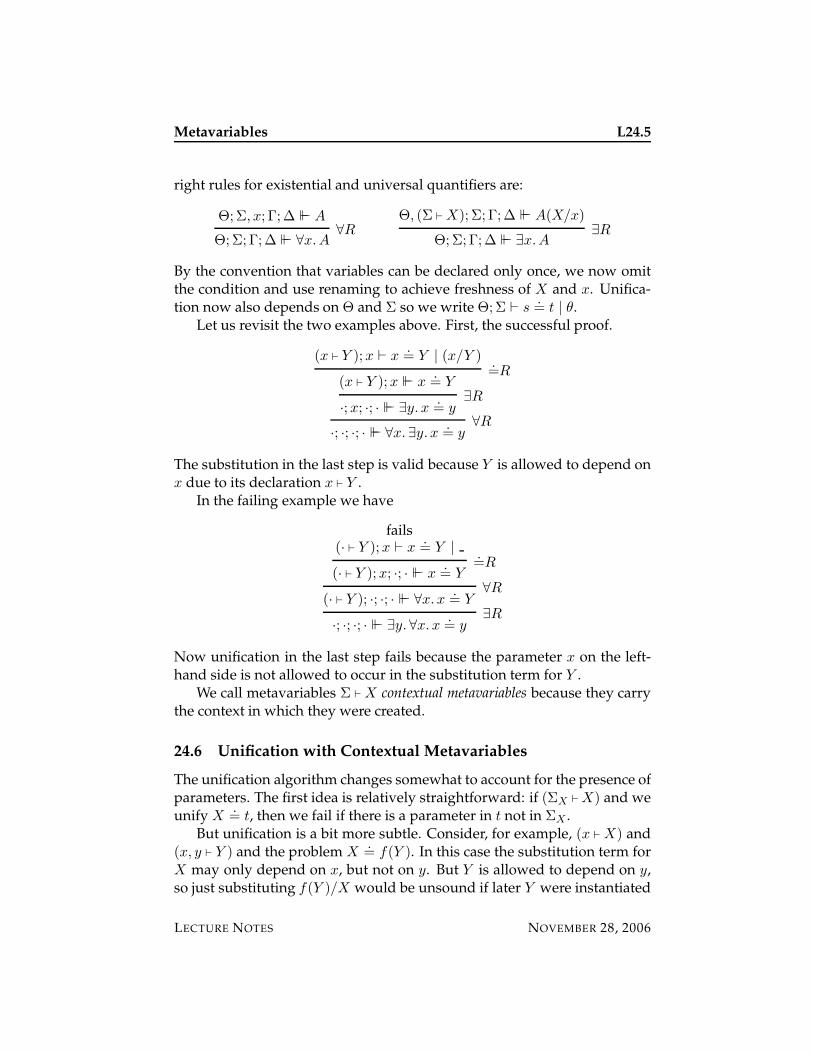
Metavariables L24.5
right rules for existential and universal quantifiers are:
Θ;Σ, x; Γ;∆ ` A
Θ;Σ; Γ;∆ ` ∀x.A∀R
Θ, (Σ ` X); Σ; Γ;∆ ` A(X/x)
Θ;Σ; Γ;∆ ` ∃x.A∃R
By the convention that variables can be declared only once, we now omitthe condition and use renaming to achieve freshness of X and x. Unifica-tion now also depends on Θ and Σ so we write Θ;Σ ` s
.= t | θ.
Let us revisit the two examples above. First, the successful proof.
(x ` Y );x ` x.= Y | (x/Y )
(x ` Y );x ` x.= Y
.=R
·;x; ·; · ` ∃y. x.= y
∃R
·; ·; ·; · ` ∀x.∃y. x.= y
∀R
The substitution in the last step is valid because Y is allowed to depend onx due to its declaration x ` Y .
In the failing example we have
fails(· ` Y );x ` x
.= Y |
(· ` Y );x; ·; · ` x.= Y
.=R
(· ` Y ); ·; ·; · ` ∀x. x.= Y
∀R
·; ·; ·; · ` ∃y.∀x. x.= y
∃R
Now unification in the last step fails because the parameter x on the left-hand side is not allowed to occur in the substitution term for Y .
We call metavariables Σ ` X contextual metavariables because they carrythe context in which they were created.
24.6 Unification with Contextual Metavariables
The unification algorithm changes somewhat to account for the presence ofparameters. The first idea is relatively straightforward: if (ΣX ` X) and weunify X
.= t, then we fail if there is a parameter in t not in ΣX .
But unification is a bit more subtle. Consider, for example, (x ` X) and(x, y ` Y ) and the problem X
.= f(Y ). In this case the substitution term for
X may only depend on x, but not on y. But Y is allowed to depend on y,so just substituting f(Y )/X would be unsound if later Y were instantiated
LECTURE NOTES NOVEMBER 28, 2006
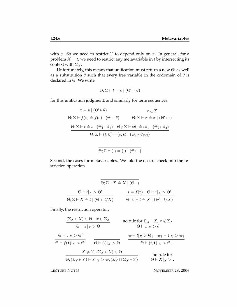
L24.6 Metavariables
with y. So we need to restrict Y to depend only on x. In general, for aproblem X
.= t, we need to restrict any metavariable in t by intersecting its
context with ΣX .
Unfortunately, this means that unification must return a new Θ′ as wellas a substitution θ such that every free variable in the codomain of θ isdeclared in Θ. We write
Θ;Σ ` t.= s | (Θ′ ` θ)
for this unification judgment, and similarly for term sequences.
t.= s | (Θ′
` θ)
Θ;Σ ` f(t).= f(s) | (Θ′
` θ)
x ∈ Σ
Θ;Σ ` x.= x | (Θ′
` ·)
Θ;Σ ` t.= s | (Θ1 ` θ1) Θ1; Σ ` tθ1
.= sθ1 | (Θ2 ` θ2)
Θ;Σ ` (t, t).= (s, s) | (Θ2 ` θ1θ2)
Θ;Σ ` (·).= (·) | (Θ ` ·)
Second, the cases for metavariables. We fold the occurs-check into the re-striction operation.
Θ;Σ ` X.= X | (Θ; ·)
Θ ` t|X > Θ′
Θ;Σ ` X.= t | (Θ′
` t/X)
t = f(t) Θ ` t|X > Θ′
Θ;Σ ` t.= X | (Θ′
` t/X)
Finally, the restriction operator:
(ΣX ` X) ∈ Θ x ∈ ΣX
Θ ` x|X > Θ
no rule for ΣX ` X, x /∈ ΣX
Θ ` x|X > θ
Θ ` t|X > Θ′
Θ ` f(t)|X > Θ′ Θ ` (·)|X > Θ
Θ ` t|X > Θ1 Θ1 ` t|X > Θ2
Θ ` (t, t)|X > Θ2
X 6= Y ; (ΣX ` X) ∈ Θ
Θ, (ΣY ` Y ) ` Y |X > Θ, (ΣY ∩ ΣX ` Y )no rule for
Θ ` X|X >
LECTURE NOTES NOVEMBER 28, 2006
Metavariables L24.7
As indicated before, restriction can fail in two ways: in x|X if x /∈ ΣX andwhen trying X|X . The first we call a parameter dependency failure, thesecond an occurs-check failure. Overall, we also call restriction an extendedoccurs-check.
24.7 Types
One of the reasons to be so pedantic in the judgments above is the nowstraightforward generalization to the typed setting. The parameter con-text Σ contains the type declarations for all the variables, and declarationΣX ` X : τ contains all the types for the parameters that may occur in thesubstitution term for X. We can take this quite far to a dependent and poly-morphic type theory and metavariables will continue to make sense. Weonly mention this here; details can be found in the literature cited below.
24.8 Higher-Order Abstract Syntax
It has been my goal in this class to present logic programming as a gen-eral paradigm of computation. It is my view that logic programming arisesfrom the study of the structure of proofs (since computation is proof search)and that model-theoretic considerations are secondary. The liberation fromthe usual concerns about Herbrand models and classical reasoning hasopened up a rich variety of new possibilities, including, for example, linearlogic programming for stateful and concurrent systems.
At the same time I have been careful to keep my own interests in appli-cations of logic programming in the background, and have drawn exam-ples from a variety of domains such as simple list manipulation, algorithmson graphs, solitaire puzzles, decision procedures, dataflow analysis, etc. Inthe remainder of this lecture and the next one I will go into some examplesof the use of logic programming in a logical framework, where the applica-tion domain itself also consists of logics and programming languages.
One of the pervasive notions in this setting is variable binding. Thenames of bound variables should not matter, and we should be able to sub-stitute for them in a way that avoids capture. For example, in a proposition∃y.∀x. x
.= y we cannot substitute x for y because the binder on x would
incorrectly capture the substitution term for y. Substitution into a quantifiedproposition is then subject to some conditions:
(∀x.A)(t/y) = ∀x.A(t/y) provided x 6= y and x /∈ FV(t).
LECTURE NOTES NOVEMBER 28, 2006
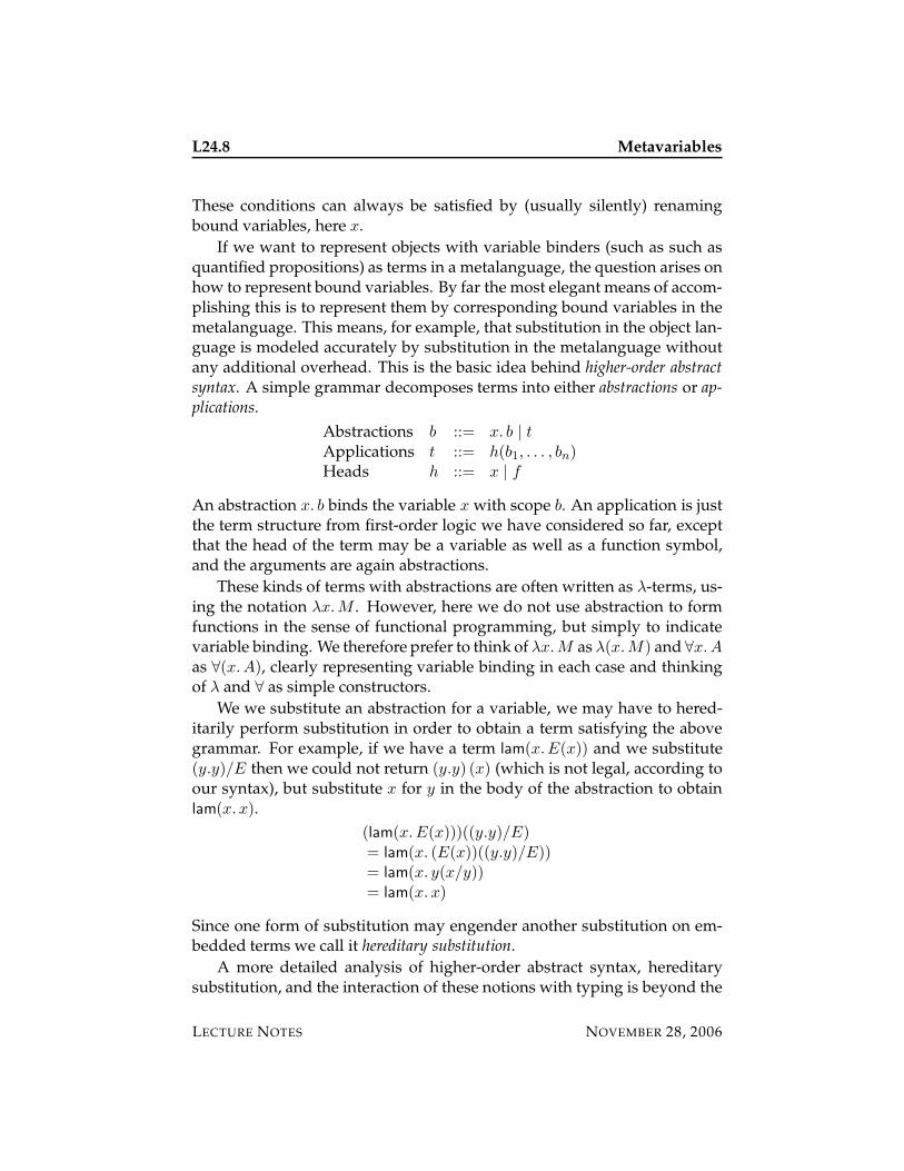
L24.8 Metavariables
These conditions can always be satisfied by (usually silently) renamingbound variables, here x.
If we want to represent objects with variable binders (such as such asquantified propositions) as terms in a metalanguage, the question arises onhow to represent bound variables. By far the most elegant means of accom-plishing this is to represent them by corresponding bound variables in themetalanguage. This means, for example, that substitution in the object lan-guage is modeled accurately by substitution in the metalanguage withoutany additional overhead. This is the basic idea behind higher-order abstractsyntax. A simple grammar decomposes terms into either abstractions or ap-plications.
Abstractions b ::= x. b | t
Applications t ::= h(b1, . . . , bn)Heads h ::= x | f
An abstraction x. b binds the variable x with scope b. An application is justthe term structure from first-order logic we have considered so far, exceptthat the head of the term may be a variable as well as a function symbol,and the arguments are again abstractions.
These kinds of terms with abstractions are often written as λ-terms, us-ing the notation λx.M . However, here we do not use abstraction to formfunctions in the sense of functional programming, but simply to indicatevariable binding. We therefore prefer to think of λx.M as λ(x.M) and ∀x.A
as ∀(x.A), clearly representing variable binding in each case and thinkingof λ and ∀ as simple constructors.
We we substitute an abstraction for a variable, we may have to hered-itarily perform substitution in order to obtain a term satisfying the abovegrammar. For example, if we have a term lam(x.E(x)) and we substitute(y.y)/E then we could not return (y.y) (x) (which is not legal, according toour syntax), but substitute x for y in the body of the abstraction to obtainlam(x. x).
(lam(x.E(x)))((y.y)/E)= lam(x. (E(x))((y.y)/E))= lam(x. y(x/y))= lam(x. x)
Since one form of substitution may engender another substitution on em-bedded terms we call it hereditary substitution.
A more detailed analysis of higher-order abstract syntax, hereditarysubstitution, and the interaction of these notions with typing is beyond the
LECTURE NOTES NOVEMBER 28, 2006
Metavariables L24.9
scope of this course. We will use it in the next lecture in order to specify theoperational semantics of a programming language.
24.9 Historical Notes
Traditionally, first-order theorem provers have used Skolemization, eitherstatically (in classical logic), or dynamically (in non-classical logics) [13].A clear presentation and solution of many issues connected to quantifierdependencies and unification has been given by Miller [5].
The idea of higher-order abstract syntax goes back to Church’s type the-ory [1] in which all variable binding was reduced to λ-abstraction. Martin-Lof’s system of arities (mostly unpublished) was a system of simple typesincluding variable binding. Its important role in logical frameworks wasidentified by several groups in 1986 and 1987, largely independently, andwith different applications: theorem proving [8], logic programming [6],and logical frameworks [2].
In programming languages, the idea of mapping bound variables in anobject language to bound variables in a metalanguage is due to Huet andLang [3]. Its use in programming environments was advocated and furtheranalyzed by Elliott and myself [11]. This paper also coined the term “higher-order abstract syntax” and is therefore sometimes falsely credited with theinvention of concept.
There are many operational issues raised by variable dependencies andhigher-order abstract syntax, most immediately unification which is impor-tant in all three types of applications (theorem proving, logic programming,and logical frameworks). The key step is Miller’s discovery of higher-orderpatterns [4] for which most general unifiers still exist. I generalized thislatter to various type theories [9, 10].
The most recent development in this area is contextual modal type the-ory [7] which gives metavariables first-class status within a type theory,rather than consider them a purely operational artifact. A presentation ofunification in a slighly simpler version of this type theory can be found inPientka’s thesis [12].
24.10 Exercises
Exercise 24.1 Show an example that leads to unsoundness if parameter depen-dency is not respected during unification using only hereditary Harrop formulas,that it, the asynchronous fragment of intuitionistic logic.
LECTURE NOTES NOVEMBER 28, 2006

L24.10 Metavariables
24.11 References
[1] Alonzo Church. A formulation of the simple theory of types. Journalof Symbolic Logic, 5:56–68, 1940.
[2] Robert Harper, Furio Honsell, and Gordon Plotkin. A framework fordefining logics. In Symposium on Logic in Computer Science, pages 194–204. IEEE Computer Society Press, June 1987.
[3] Gerard Huet and Bernard Lang. Proving and applying program trans-formations expressed with second-order patterns. Acta Informatica,11:31–55, 1978.
[4] Dale Miller. A logic programming language with lambda-abstraction,function variables, and simple unification. Journal of Logic and Compu-tation, 1(4):497–536, 1991.
[5] Dale Miller. Unification under a mixed prefix. Journal of Symbolic Com-putation, 14:321–358, 1992.
[6] Dale Miller, Gopalan Nadathur, and Andre Scedrov. Hereditary Har-rop formulas and uniform proof systems. In David Gries, editor, Sym-posium on Logic in Computer Science, pages 98–105, Ithaca, NY, June1987.
[7] Aleksandar Nanevski, Frank Pfenning, and Brigitte Pientka. Contex-tual modal type theory. Submitted, September 2005.
[8] Lawrence C. Paulson. Natural deduction as higher-order resolution.Journal of Logic Programming, 3:237–258, 1986.
[9] Frank Pfenning. Logic programming in the LF logical framework. InGerard Huet and Gordon Plotkin, editors, Logical Frameworks, pages149–181. Cambridge University Press, 1991.
[10] Frank Pfenning. Unification and anti-unification in the Calculus ofConstructions. In Sixth Annual IEEE Symposium on Logic in ComputerScience, pages 74–85, Amsterdam, The Netherlands, July 1991.
[11] Frank Pfenning and Conal Elliott. Higher-order abstract syntax. InProceedings of the ACM SIGPLAN ’88 Symposium on Language Designand Implementation, pages 199–208, Atlanta, Georgia, June 1988.
[12] Brigitte Pientka. Tabled Higher-Order Logic Programming. PhD thesis,Department of Computer Science, Carnegie Mellon University, De-cember 2003. Available as Technical Report CMU-CS-03-185.
LECTURE NOTES NOVEMBER 28, 2006
Metavariables L24.11
[13] N. Shankar. Proof search in the intuitionistic sequent calculus. InD. Kapur, editor, Proceedings of the 11th International Conference on Au-tomated Deduction (CADE-11), pages 522–536, Saratoga Springs, NewYork, June 1992. Springer-Verlag LNCS 607.
LECTURE NOTES NOVEMBER 28, 2006

L24.12 Metavariables
LECTURE NOTES NOVEMBER 28, 2006
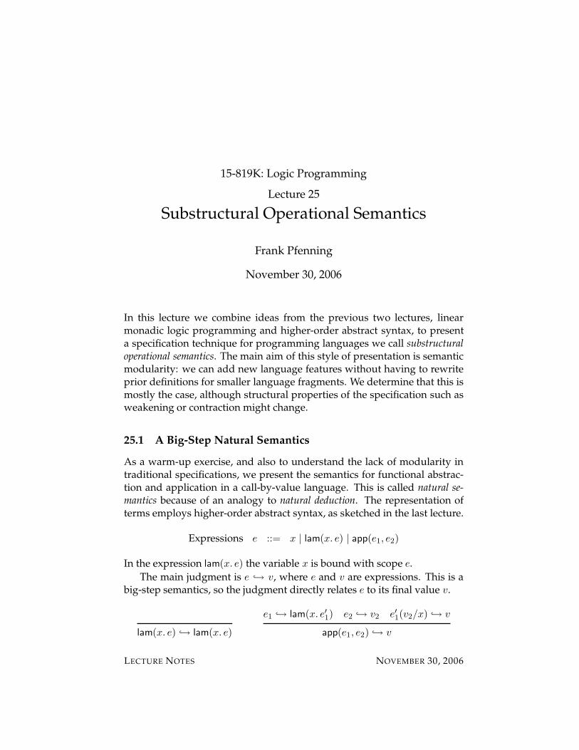
15-819K: Logic Programming
Lecture 25
Substructural Operational Semantics
Frank Pfenning
November 30, 2006
In this lecture we combine ideas from the previous two lectures, linearmonadic logic programming and higher-order abstract syntax, to presenta specification technique for programming languages we call substructuraloperational semantics. The main aim of this style of presentation is semanticmodularity: we can add new language features without having to rewriteprior definitions for smaller language fragments. We determine that this ismostly the case, although structural properties of the specification such asweakening or contraction might change.
25.1 A Big-Step Natural Semantics
As a warm-up exercise, and also to understand the lack of modularity intraditional specifications, we present the semantics for functional abstrac-tion and application in a call-by-value language. This is called natural se-mantics because of an analogy to natural deduction. The representation ofterms employs higher-order abstract syntax, as sketched in the last lecture.
Expressions e ::= x | lam(x. e) | app(e1, e2)
In the expression lam(x. e) the variable x is bound with scope e.
The main judgment is e ↪→ v, where e and v are expressions. This is abig-step semantics, so the judgment directly relates e to its final value v.
lam(x. e) ↪→ lam(x. e)
e1 ↪→ lam(x. e′1) e2 ↪→ v2 e′
1(v2/x) ↪→ v
app(e1, e2) ↪→ v
LECTURE NOTES NOVEMBER 30, 2006
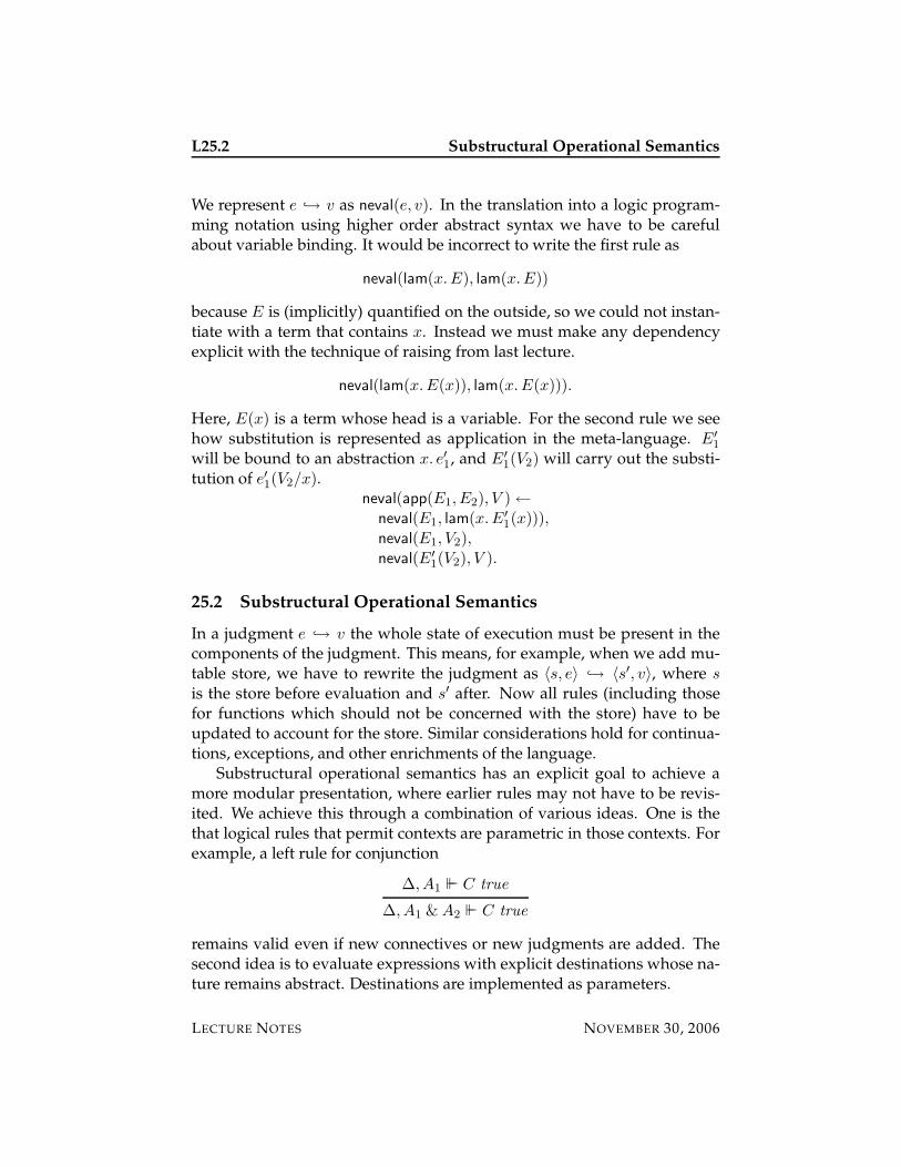
L25.2 Substructural Operational Semantics
We represent e ↪→ v as neval(e, v). In the translation into a logic program-ming notation using higher order abstract syntax we have to be carefulabout variable binding. It would be incorrect to write the first rule as
neval(lam(x.E), lam(x.E))
because E is (implicitly) quantified on the outside, so we could not instan-tiate with a term that contains x. Instead we must make any dependencyexplicit with the technique of raising from last lecture.
neval(lam(x.E(x)), lam(x.E(x))).
Here, E(x) is a term whose head is a variable. For the second rule we seehow substitution is represented as application in the meta-language. E′
1
will be bound to an abstraction x. e′1, and E′
1(V2) will carry out the substi-
tution of e′1(V2/x).
neval(app(E1, E2), V )←neval(E1, lam(x.E′
1(x))),
neval(E1, V2),neval(E′
1(V2), V ).
25.2 Substructural Operational Semantics
In a judgment e ↪→ v the whole state of execution must be present in thecomponents of the judgment. This means, for example, when we add mu-table store, we have to rewrite the judgment as 〈s, e〉 ↪→ 〈s′, v〉, where s
is the store before evaluation and s′ after. Now all rules (including thosefor functions which should not be concerned with the store) have to beupdated to account for the store. Similar considerations hold for continua-tions, exceptions, and other enrichments of the language.
Substructural operational semantics has an explicit goal to achieve amore modular presentation, where earlier rules may not have to be revis-ited. We achieve this through a combination of various ideas. One is thethat logical rules that permit contexts are parametric in those contexts. Forexample, a left rule for conjunction
∆, A1 ` C true
∆, A1 & A2 ` C true
remains valid even if new connectives or new judgments are added. Thesecond idea is to evaluate expressions with explicit destinations whose na-ture remains abstract. Destinations are implemented as parameters.
LECTURE NOTES NOVEMBER 30, 2006
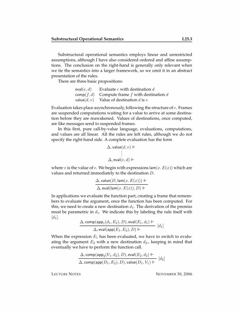
Substructural Operational Semantics L25.3
Substructural operational semantics employs linear and unrestrictedassumptions, although I have also considered ordered and affine assump-tions. The conclusion on the right-hand is generally only relevant whenwe tie the semantics into a larger framework, so we omit it in an abstractpresentation of the rules.
There are three basic propositions:
eval(e, d) Evaluate e with destination d
comp(f, d) Compute frame f with destination d
value(d, v) Value of destination d is v
Evaluation takes place asynchronously, following the structure of e. Framesare suspended computations waiting for a value to arrive at some destina-tion before they are reawakened. Values of destinations, once computed,are like messages send to suspended frames.
In this first, pure call-by-value language, evaluations, computations,and values are all linear. All the rules are left rules, although we do notspecify the right-hand side. A complete evaluation has the form
∆, value(d, v) `....
∆, eval(e, d) `
where v is the value of e. We begin with expressions lam(x.E(x)) which arevalues and returned immediately to the destination D.
∆, value(D, lam(x.E(x))) `
∆, eval(lam(x.E(x)),D) `
In applications we evaluate the function part, creating a frame that remem-bers to evaluate the argument, once the function has been computed. Forthis, we need to create a new destination d1. The derivation of the premissmust be parametric in d1. We indicate this by labeling the rule itself with[d1].
∆, comp(app1(d1, E2),D), eval(E1, d1) `
∆, eval(app(E1, E2),D) `[d1]
When the expression E1 has been evaluated, we have to switch to evalu-ating the argument E2 with a new destination d2., keeping in mind thateventually we have to perform the function call.
∆, comp(app2(V1, d2),D), eval(E2, d2) `
∆, comp(app(D1, E2),D), value(D1, V1) `[d2]
LECTURE NOTES NOVEMBER 30, 2006
L25.4 Substructural Operational Semantics
It may be possible to reuse the destination D1, but we are not interestedhere in this kind of optimization. It might also interfere negatively withextensibility later on if destinations are reused in this manner.
Finally, the β-reduction when both function and argument are known.
∆, eval(E′
1(V2),D) `
∆, comp(app2(lam(x.E′
1(x)),D2),D), value(D2, V2) `
25.3 Substructural Operational Semantics in LolliMon
It is easy to take the four rules of our substructural specification and imple-ment them in LolliMon. We need here linear forward chaining and existen-tial quantification to introduce new destinations. LolliMon’s term languagepermits abstraction, so we can use this to implement higher-order abstractsyntax.
eval(lam(x.E(x)),D) ( {value(D, lam(x.E(x)))}.
eval(app(E1, E2),D) ( {∃d1. eval(E1, d1)⊗ comp(app1(d1, E2),D)}.
value(D1, V1)⊗ comp(app1(D1, E2),D)( {∃d2. eval(E2, d2)⊗ comp(app2(V1, d2),D)}.
value(D2, V2)⊗ comp(app2(lam(x.E′
1(x)),D2),D) ( {eval(E′
1(V2),D)}.
The only change we have made to the earlier specification is to exchangethe order of eval, comp, and value propositions for a more natural threadingof destinations.
LolliMon combines forward and backward chaining, so we can alsowrite the top-level judgment to obtain the final value.
evaluate(E,V ) ◦− (∀d0. eval(E, d0) ( {value(d0, V )}).
25.4 Adding Mutable Store
We would now like to add mutable store to the operational semantics. Wehave three new kinds of expressions to create, read, and assign to a cell ofmutable storage.
Expressions e ::= . . . | ref(e) | deref(e) | assign(e1, e2) | cell(c)
There is also a new kind of value cell(c) where c is a destination whichserves as a name for a cell of storage. Note that cell(c) cannot appear in the
LECTURE NOTES NOVEMBER 30, 2006
Substructural Operational Semantics L25.5
source. In order to enforce this syntactically we would distinguish a type ofvalues from the type of expressions, something we avoid here for the sakeof brevity.
First, the rules for creating a new cell. I suggest reading these rulesfrom last to first, in the way they will be used in a computation. We writethe destinations that model cells at the left-hand side of the context. This isonly a visual aid and has no logical significance.
value(c1, V1),∆, value(D, cell(c1)) `
∆, comp(ref1(D1),D), value(D1, V1) `[c1]
∆, comp(ref1(d1),D), eval(E1, d1) `
∆, eval(ref(E1),D) `[d1]
We keep track of the value of in a storage cell with an assumption value(c, v)where c is a destination and v is a value. While destinations to be usedas cells are modeled here as linear, they are in reality affine, that is, theymay be used at most once. The store, which is represented by the set ofassumptions value(ci, vi) will remain until the end of the computation.
Next, reading the value of a cell. Again, read the rules from the bottomup, and the last rule first.
value(C1, V1),∆, value(D,V1) `
value(C1, V1),∆, comp(deref1(D1),D), value(D1, cell(C1)) `
∆, comp(deref1(d1),D), eval(E1, d1) `
∆, eval(deref(E1),D) `[d1]
Next, assigning a value to a cell. The assignment assign(e1, e2) returns thevalue of e2.
value(C1, V2), value(D,V2) `
value(C1, V1),∆, comp(assign2(cell(C1),D2),D), value(D2, V2) `
∆, comp(assign2(V1, d2),D), eval(E2, d2) `
∆, comp(assign1(D1, E2),D), value(D1, V1) `[d2]
∆, comp(assign1(d1, E2),D), eval(E1, d1) `
∆, eval(assign(E1, E2),D) `[d1]
LECTURE NOTES NOVEMBER 30, 2006
L25.6 Substructural Operational Semantics
Because values are included in expressions, we need one more rule for cells(which are treated as values). Even if they do not occur in expressionsinitially, the arise from substitutions of values into expressions.
∆, value(D, cell(C)) `
∆, eval(cell(C),D) `
All of these rules are just added to the previous rules for functions. Wehave achieved semantic modularity, at least for functions and store.
Again, it is easy to turn these rules into a LolliMon program.
eval(ref(E1),D)( {∃d1. eval(E1, d1)⊗ comp(ref1(d1),D)}.
value(D1, V1)⊗ comp(ref1(D1),D)( {∃c1. value(c1, V1)⊗ value(D, cell(c1))}.
eval(deref(E1),D)( {∃d1. eval(E1, d1)⊗ comp(deref1(d1),D)}.
value(D1, cell(C1))⊗ value(C1, V1)⊗ comp(deref1(D1),D)( {value(C1, V1)⊗ value(D,V1)}.
eval(assign(E1, E2),D)( {∃d1. eval(E1, d1)⊗ comp(assign1(d1, E2),D)}.
value(D1, V1)⊗ comp(assign1(D1, E2),D)( {∃d2. eval(E2, d2)⊗ comp(assign2(V1, d2),D)}.
value(D2, V2)⊗ comp(assign2(cell(C1),D2),D)⊗ value(C1, V1)( {value(C1, V2)⊗ value(D,V2)}.
eval(cell(C),D)( {value(D, cell(C))}.
Written in SSOS form, the program evaluates e with some initial desti-nation d0 as
∆, value(d0, v) `....
eval(e, d0) `
where v is the value of e and
∆ = value(c1, v1), . . . , value(cn, vn)
LECTURE NOTES NOVEMBER 30, 2006
Substructural Operational Semantics L25.7
for cells c1, . . . , cn. The matter is complicated further by the fact that ci, pa-rameters introduced during the deduction, may appear in v. So we wouldhave to traverse v to eliminate references to ci, or we could just print it, orwe could create some form of closure over the store ∆. In either case, weneed to be sure to comsume ∆ to retain linearity overall. If we just want tocheck termination, the top-level program would be
terminates(E) ◦− ∀d0. eval(E, d0) ( {∃V. value(d0, V )⊗>}.
Here, the existential quantifier will be instantiated after forward chainingreaches quiescence, so it is allowed to depend on all the parameters intro-duced during forward chaining.
25.5 Adding Continuations
We now add callcc to capture the current continuation and throw to invokea continuation as an example of an advanced control-flow construct.
Expressions e ::= . . . | callcc(x. e) | throw(e1, e2) | cont(d)
The intuitive meaning is that callcc(x. e) captures the current continuation(represented as the value cont(d)) and substitutes it for x in e, and thatthrow(e1, e2) evaluates e1 to v1, e2 to a continuation k and then invokes k onv1.
In linear destination-passing style, we use a destination d to stand fora continuation. We invoke a continuation d on a value v simply by settingvalue(d, v). Any frame waiting to receive a value can be activated in thismanner.
But this creates several problems in the semantics. To illustrate them,we add z and s(e) for zero and successor, and a new frame s1(d) whichwaits to increment the value returned to destination d. See Exercise 25.2 forthe rules.
Then an expression
s(callcc(k. s(throw(z, k))))
evaluates to s(z), never returning anything to the inner frame waiting tocalculate a successor. This means frames are no longer linear—they may beignored and therefore be left over at the end.
But the problems do not end there. Consider, for example,
app(callcc(k. lam(x. throw(lam(y. y), k))), z).
LECTURE NOTES NOVEMBER 30, 2006
L25.8 Substructural Operational Semantics
Because any λ-expression is a value, the callcc returns immediately andapplies the function lam(x. . . .) to z. This causes the embedded throw totake place, this time applying lam(y. y) to z, yielding z as the final value. Inthis computation, the continuation in place when the first argument to app
is evaluated is invoked twice: first, because we return to it, and then againwhen we throw to it. This means frames may not only be ignored, but alsoduplicated.
The solution is to make all frames comp(f, d) unrestricted throughout.At the same time the other predicates must remain linear: eval(e, d) so thatthere is only one thread of computation, and value(d, v) so that at any giventime there is at most one value v at any given destination d.
We present the semantics for callcc and related constructs directly inLolliMon, which is more compact than the inference rule presentation.
eval(callcc(k.E(k)),D)( {eval(E(cont(D)),D)}.
eval(throw(E1, E2),D)( {∃d1. eval(E1, d1)⊗ !comp(throw1(d1, E2),D)}.
value(D1, V1)⊗ !comp(throw1(D1, E2),D)( {∃d2. eval(E2, d2)⊗ !comp(throw2(V1, d2),D)}.
value(D2, cont(D′
2))⊗ !comp(throw2(V1,D2),D)
( {value(D′
2, V1)}.
eval(cont(D′),D)( {value(D, cont(D′))}.
Of course, all other rules so far must be modified to make the suspendedcomputations (which we now recognize as continuations) unrestricted byprefixing each occurrence of comp(f, d) with ‘!’. The semantics is not quitemodular in this sense.
With this change we have functions, mutable store, and continuationsin the same semantics, specified in the form of a substructural operationalsemantics.
25.6 Substructural Properties Revisited
The only aspect of our specification we had to revise was the substructuralproperty of suspended computations. If we step back we see that we canuse substructural properties of various language features for a kind of tax-onomy.
LECTURE NOTES NOVEMBER 30, 2006
Substructural Operational Semantics L25.9
Our first observation is that for functions alone it would have been suf-ficient to keep the suspended computations next to each other and in or-der. In such an ordered specification we would not even have needed thedestinations, because adjacency guarantees that values arrive at proper lo-cations. We will leave this observation informal, rather than introducing aversion of LolliMon with an ordered context, although this would clearlybe possible.
If we add mutable store, then propositions value(d, v) remain linear,while propositions value(c, v) for destinations d that act as cells are affine.Continuations comp(f, d) are still linear, as are propositions eval(e, d).
If we further add a means to capture the continuation, then suspendedcomputations comp(f, d) must become unrestricted because we may eitherignore a continuation or return to it more than once. Values value(d, v) mustremain linear, as must evaluations eval(e, d). Storage cells remain affine.
With sufficient foresight we could have made suspended computationscomp(f, d) unrestricted to begin with. Nothing in the early semantics relieson their linearity. On other hand, it is more interesting to see what struc-tural properties would and would not work for various languages, and alsomore natural to assume only the properties that are necessary.
25.7 Historical Notes
The presentation of a big-step operational semantics relating an expressionto its value by inference rules is due to Kahn [2] under the name naturalsemantics. Earlier, Plotkin [6] developed a presentation of operational se-mantics using rewrite rules following the structure of expressions underthe name structural operational semantics (SOS). I view substructural opera-tional semantics as a further development and extension of SOS. Anothergeneralization to achieve modularity is Mosses’ modular structural opera-tional semantics [4] which uses top-down logic programming and a formof row polymorphism for extensibility.
To my knowledge, the first presentation of an operational semanticsin linear destination-passing style appeared as an example for the use ofthe Concurrent Logical Framework (CLF) [1]. The formulation there wasintrinsically of higher order, which made reasoning about the rules moredifficult. The approach was formulated as an independent technique formodular language specification in an invited talk [5], but only an abstractwas published. Further examples of substructural operational semanticswere given in the paper that introduced LolliMon [3].
LECTURE NOTES NOVEMBER 30, 2006
L25.10 Substructural Operational Semantics
Using ordered assumptions in logical frameworks and logic program-ming was proposed by Polakow and myself [8, 7], although this work didnot anticipate monadic forward chaining as a computational mechanism.
25.8 Exercises
Exercise 25.1 Prove that the natural semantics and substructural semantics forthe functional fragment coincide in a suitable sense.
Exercise 25.2 Add natural number constants z and s(e) to our language specifi-cation to permit more examples for callcc. Give formulations both in substructuraloperational semantics and in LolliMon.
Exercise 25.3 Extend the functional language with unit, pairs, sums, void, andrecursive types as well as recursion at the level of expressions. Give a substructuraloperational semantics directly in LolliMon.
Exercise 25.4 Think of other interesting control constructs, for example, for par-allel or concurrent computation, and represent them in substructural operationalsemantics.
Exercise 25.5 Give a specification of a call-by-value language where we do notsubstitute a complete value for a term, but only the name for the destination whichholds the (immutable) value. Which is the proper substructural property for suchdestinations?
Further extend this idea to capture a call-by-need semantics where argumentsare evaluated the first time they are needed and then memoized. This is the seman-tics underlying lazy functional languages such as Haskell.
25.9 References
[1] Iliano Cervesato, Frank Pfenning, David Walker, and Kevin Watkins. Aconcurrent logical framework II: Examples and applications. TechnicalReport CMU-CS-02-102, Department of Computer Science, CarnegieMellon University, 2002. Revised May 2003.
[2] Gilles Kahn. Natural semantics. In Proceedings of the Symposium on The-oretical Aspects of Computer Science, pages 22–39. Springer-Verlag LNCS247, 1987.
LECTURE NOTES NOVEMBER 30, 2006
Substructural Operational Semantics L25.11
[3] Pablo Lopez, Frank Pfenning, Jeff Polakow, and Kevin Watkins. Mon-adic concurrent linear logic programming. In A.Felty, editor, Proceed-ings of the 7th International Symposium on Principles and Practice of Declar-ative Programming (PPDP’05), pages 35–46, Lisbon, Portugal, July 2005.ACM Press.
[4] Peter D. Mosses. Foundations of modular SOS. In Proceedings of the24th International Symposium on Mathematical Foundations of ComputerScience (MFCS’99), pages 70–80, Szklarska Poreba, Poland, September1999. Springer-Verlag LNCS 1672. Extended version available as BRICSResearch Series RS-99-54, University of Aarhus.
[5] Frank Pfenning. Substructural operational semantics and linear dest-ination-passing style. In Wei-Ngan Chin, editor, Proceedings of the 2ndAsian Symposium on Programming Languages and Systems (APLAS’04),page 196, Taipei, Taiwan, November 2004. Springer-Verlag LNCS 3302.
[6] Gordon D. Plotkin. A structural approach to operational seman-tics. Technical Report DAIMI FN-19, Computer Science Department,Aarhus University, Aarhus, Denmark, September 1981.
[7] Jeff Polakow. Ordered Linear Logic and Applications. PhD thesis, Depart-ment of Computer Science, Carnegie Mellon University, August 2001.
[8] Jeff Polakow and Frank Pfenning. Relating natural deduction and se-quent calculus for intuitionistic non-commutative linear logic. In An-dre Scedrov and Achim Jung, editors, Proceedings of the 15th Conferenceon Mathematical Foundations of Programming Semantics, New Orleans,Louisiana, April 1999. Electronic Notes in Theoretical Computer Sci-ence, Volume 20.
LECTURE NOTES NOVEMBER 30, 2006

L25.12 Substructural Operational Semantics
LECTURE NOTES NOVEMBER 30, 2006
15-819K: Logic Programming
Lecture 26
Datalog
Frank Pfenning
December 5, 2006
In this lecture we describe Datalog, a decidable fragment of Horn logic.Briefly, Datalog disallows function symbols, which means that the so-calledHerbrand universe of ground instances of predicates is finite. Datalog hasapplications in databases and, more recently, in program analysis and re-lated problems. We also sketch a promising new way to implement Datalogvia its bottom-up semantics using BDDs to represent predicates.
26.1 Stratified Negation
Datalog arises from Horn logic via two restrictions and an extension. Themost important restriction is to disallow function symbols: terms must bevariables or be drawn from a fixed set of constant symbols. The secondrestriction is that any variable in the head of a clause also appears in thebody. Together these mean that all predicates are decidable via a simplebottom-up, forward chaining semantics, since there are only finitely manypropositions that can arise. These propositions form the so-called Herbranduniverse.
If all domains of quantification are finite, we can actually drop the re-striction on variables in clause heads, since a head such as p(x) just standsfor finitely many instances p(c1), . . . , p(cn), where c1, . . . , cn is an enumera-tion of the elements of the domain of p.
In either case, the restriction guarantees decidability. This means it ispossible to add a sound form of constructive negation, called stratified nega-tion. For predicates p and q we say p directly depends on q if the body of aclause with head p(t) contains q(s). We write p ≥ q for the reflexive andtransitive closure of the direct dependency relation. If q does not depend
LECTURE NOTES DECEMBER 5, 2006
L26.2 Datalog
on p then we can decide any atom q(s) without reference to the predicate p.This allows us to write clauses such as
p(t)← . . . ,¬q(s), . . .
without ambiguity: first we can determine the extension of q and then con-clude ¬q(s) for ground term s if q(s) was not found to be true.
If the domains are infinite, or we want to avoid potentially explosiveexpansion of schematics facts, we must slightly refine our restrictions frombefore: any goal ¬q(s) should be such that s is ground when we have todecide it, so it can be implemented by a lookup assuming that q has alreadybeen saturated.
A Datalog program which is stratified in this sense can be saturatedby sorting the predicates into a strict partial dependency order and thenproceeding bottom-up, saturating all predicates lower in the order beforemoving on to predicates in a higher stratum.
Programs that are not stratified, such as
p← ¬p.
orp← ¬q.
q ← ¬p.
do not have such a clear semantics and are therefore disallowed. However,many technical variations of the most basic one given above have beenconsidered in the literature.
26.2 Transitive Closure
A typical use of Datalog is the computation of the transitive closure of arelation. We can also think of this as computing reachability in a directedgraph given the definition of the edge relation.
In the terminology of Datalog, the extensional data base (EDB) is given byexplicit (ground) propositions p(t). The intensional data base (IDB) is givenby Datalog rules, including possible stratified uses of negation.
In the graph reachability example, the EDB consists of propositionsedge(x, y) for nodes x and y defining the edge relation. The path relation,which is the transitive closure of the edge relation, is defined by two ruleswhich constitute the IDB.
path(x, y)← edge(x, y).path(x, y)← path(x, z), path(z, y).
LECTURE NOTES DECEMBER 5, 2006
Datalog L26.3
26.3 Liveness Analysis, Revisited
As another example of the use of Datalog, we revisit the earlier problem ofprogram analysis in a small imperative language.
l : x = op(y, z)l : if x goto k
l : goto k
l : halt
We say a variable is live at a given program point l if its value will be readbefore it is written when computation reaches l. Following McAllester, wewrote a bottom-up logic program for liveness analysis and determined itscomplexity using prefix firings as O(v·n) where v is the number of variablesand n the number of instructions in the program.
This time we take a different approach, mapping the problem to Data-log. The idea is to extract from the program propositions in the initial EDBof the following form:
• read(x, l). Variable x is read at line l.
• write(x, l). Variables x is written at line l.
• succ(l, k). Line k is a (potential) successor to line l.
The succ predicate depends on the control flow of the program so, for ex-ample, conditional jump instructions have more than one successor. In ad-dition we will define by rules (and hence in the IDB) the predicate:
• live(x, l). Variable x may be live at line l.
Like most program analyses, this is a conservative approximation: we mayconclude that a variable x is live at l, but it will never actually be read. Onthe other hand, if live(x, l) is not true, then we know for sure that x cannever be live at l. This sort of information may be used by compilers inregister allocation and optimizations.
First, we describe the extraction of the EDB from the program. Everyprogram instruction expands into a set of assertions about the program
LECTURE NOTES DECEMBER 5, 2006
L26.4 Datalog
lines and program variables.
l : x = op(y, z) ↔
read(y, l)read(z, l)write(x, l)succ(l, l + 1)
l : if x goto k ↔
read(x, l)succ(l, k)succ(l, l + 1)
l : goto k ↔ succ(l, k)
l : halt ↔ none
Here we assume that the next line l+1 is computed explicitly at translationtime.
Now the whole program analysis can be defined by just two Datalogrules.
live(w, l) ← read(w, l).live(w, l) ← live(w, k), succ(k, l),¬write(w, l).
The program is stratified in that live depends on read, write, and succ butnot vice versa. Therefore the appeal to negation in the second clause islegitimate.
This is an extremely succinct and elegant expression of liveness anal-ysis. Interestingly, it also provides a practical implementation as we willdiscuss in the remainder of this lecture.
26.4 Binary Decision Diagrams
There are essentially two “traditional” ways of implementing Datalog: oneis by a bottom-up logic programming engine, the other using a top-downlogic programming engine augmented with tabling in order to avoid non-termination. Recently, a new mechanism has been proposed using binarydecision diagrams, which has been shown to be particularly effective in largescale program analysis.
We briefly review here binary decision diagrams (BDDs). To be moreprecise, we will sketch the basics of reduced ordered binary decision diagrams(ROBDDs) which are most useful in this context for reasons we will illus-trate below.
LECTURE NOTES DECEMBER 5, 2006
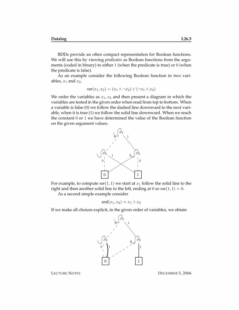
Datalog L26.5
BDDs provide an often compact representation for Boolean functions.We will use this by viewing predicates as Boolean functions from the argu-ments (coded in binary) to either 1 (when the predicate is true) or 0 (whenthe predicate is false).
As an example consider the following Boolean function in two vari-ables, x1 and x2.
xor(x1, x2) = (x1 ∧ ¬x2) ∨ (¬x1 ∧ x2)
We order the variables as x1, x2 and then present a diagram in which thevariables are tested in the given order when read from top to bottom. Whena variable is false (0) we follow the dashed line downward to the next vari-able, when it is true (1) we follow the solid line downward. When we reachthe constant 0 or 1 we have determined the value of the Boolean functionon the given argument values.
GFED@ABC x1
0
��
��
� 1
8888
8888
88
GFED@ABC x2
0
���� 1
KKKKKKKKKKKKKKKKGFED@ABC x2
1
ssssssssssssssss0
����
0 1
For example, to compute xor(1, 1) we start at x1 follow the solid line to theright and then another solid line to the left, ending at 0 so xor(1, 1) = 0.
As a second simple example consider
and(x1, x2) = x1 ∧ x2
If we make all choices explicit, in the given order of variables, we obtain
GFED@ABC x1
0
��
��
� 1
8888
8888
88
GFED@ABC x2
0��
&
1
GFED@ABC x20
ss
ss
ss
ss
1
0 1
LECTURE NOTES DECEMBER 5, 2006
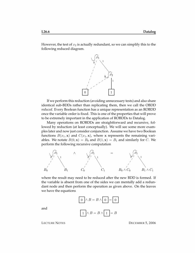
L26.6 Datalog
However, the test of x2 is actually redundant, so we can simplify this to thefollowing reduced diagram.
GFED@ABC x1
0
���������� 1
8888
8888
88
GFED@ABC x20
tt
tt
tt
tt
1
0 1
If we perform this reduction (avoiding unnecessary tests) and also shareidentical sub-BDDs rather than replicating them, then we call the OBDDreduced. Every Boolean function has a unique representation as an ROBDDonce the variable order is fixed. This is one of the properties that will proveto be extremely important in the application of ROBDDs to Datalog.
Many operations on ROBDDs are straightforward and recursive, fol-lowed by reduction (at least conceptually). We will see some more exam-ples later and now just consider conjunction. Assume we have two Booleanfunctions B(x1,x) and C(x1,x), where x represents the remaining vari-ables. We notate B(0,x) = B0 and B(1,x) = B1 and similarly for C . Weperform the following recursive computation
GFED@ABC x1
0
��
��� 1
3333
3333
3
B0 B1
∧ GFED@ABC x1
0
�����
1
2222
2222
2
C0 C1
= GFED@ABC x1
0
1
5555
5555
5
B0 ∧ C0 B1 ∧ C1
where the result may need to be reduced after the new BDD is formed. Ifthe variable is absent from one of the sides we can mentally add a redun-dant node and then perform the operation as given above. On the leaveswe have the equations
0 ∧B = B ∧ 0 = 0
and
1 ∧B = B ∧ 1 = B
LECTURE NOTES DECEMBER 5, 2006
Datalog L26.7
Other Boolean operations propagate in the same way; only the actions onthe leaves are different in each case.
There are further operations which we sketch below in the example aswe need them.
26.5 Datalog via ROBDDs
When implementing Datalog via ROBDDs we represent every predicateas a Boolean function. This is done in two steps: based on the type ofthe argument, we find out how many distinct constants can appear in thisargument (say n) and then represent them with log2(n) bits. The output ofthe function is always 1 or 0, depending on whether the predicate is true(1) or false (0). In this way we can represent the initial EDB as a collectionof ROBDDs, one for each predicate.
Now we need to apply the rules in the IDB in a bottom-up manner untilwe have reached saturation. We achieve this by successive approximation,starting with the everywhere false predicate or some initial approximationbased on the EDB. Then we compute the Boolean function correspondingto the body of each clause and combine it disjunctively with the current ap-proximation. When the result turns out to be equal to the previous approx-imation we stop: saturation has been achieved. Fortunately this equality iseasy to detect, since Boolean functions have unique representations.
We discuss the kind of operations required to compute the body ofeach clause only by example. Essentially, they are relabeling of variables,Boolean combinations such as conjunction and disjunction, and projection(which becomes an existential quantification).
As compared to traditional bottom-up strategy, where each fact is repre-sented separately, we iterate over the whole current approximation of thepredicate in each step. If the information is regular, this leads to a lot ofsharing which can indeed be observed in practice.
26.6 An Example of Liveness Analysis
Now we walk through a small example of liveness analysis in detail in or-der to observe the BDD implementation of Datalog in action. Our programis very simple.
l0 : w0 = w1 + w1
l1 : if w0 goto l0l2 : halt
LECTURE NOTES DECEMBER 5, 2006
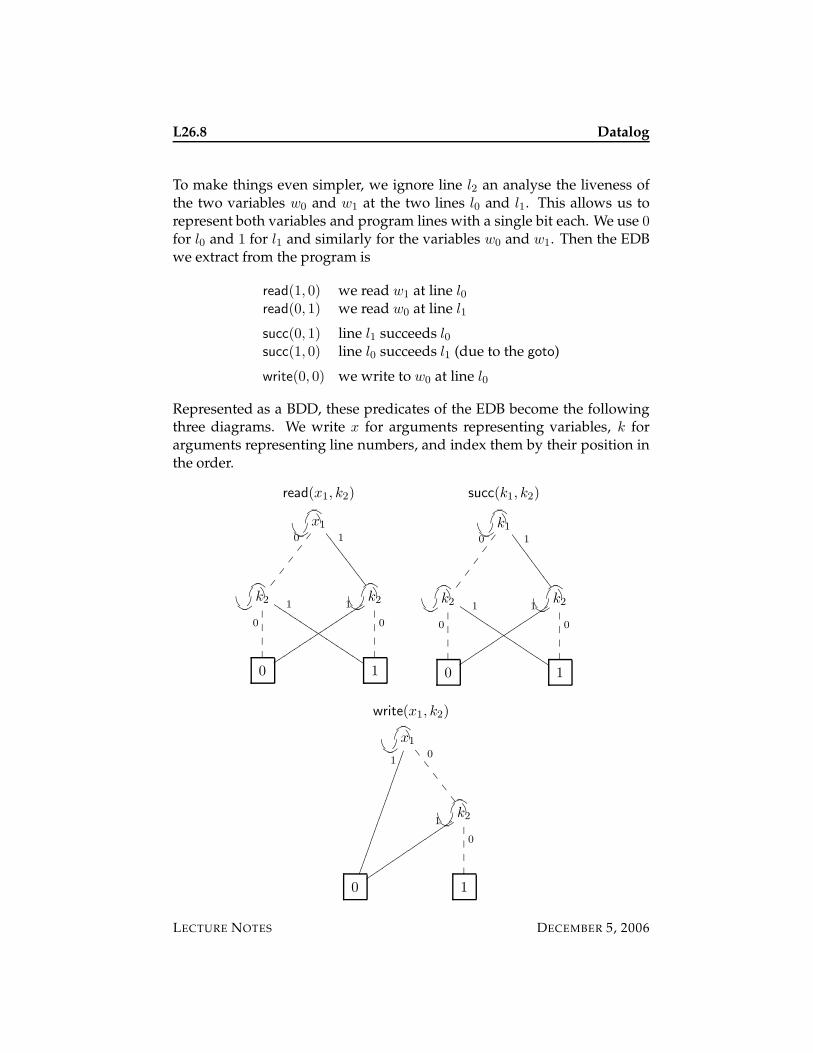
L26.8 Datalog
To make things even simpler, we ignore line l2 an analyse the liveness ofthe two variables w0 and w1 at the two lines l0 and l1. This allows us torepresent both variables and program lines with a single bit each. We use 0for l0 and 1 for l1 and similarly for the variables w0 and w1. Then the EDBwe extract from the program is
read(1, 0) we read w1 at line l0read(0, 1) we read w0 at line l1
succ(0, 1) line l1 succeeds l0succ(1, 0) line l0 succeeds l1 (due to the goto)
write(0, 0) we write to w0 at line l0
Represented as a BDD, these predicates of the EDB become the followingthree diagrams. We write x for arguments representing variables, k forarguments representing line numbers, and index them by their position inthe order.
read(x1, k2) succ(k1, k2)
GFED@ABC x1
0
��
��
� 1
8888
8888
88
GFED@ABC k2
0
���� 1
JJJJJJJJJJJJJJJJJGFED@ABC k2
1
ttttttttttttttttt
0
����
0 1
GFED@ABC k1
0
��
��
� 1
7777
7777
77
GFED@ABC k2
0
���� 1
JJJJJJJJJJJJJJJJGFED@ABC k2
1
tttttttttttttttt
0
����
0 1
write(x1, k2)
GFED@ABC x1
1
�������������������� 0
88
88
8
GFED@ABC k21
uuuuuuuuuuuuuuuu
0
����
0 1
LECTURE NOTES DECEMBER 5, 2006
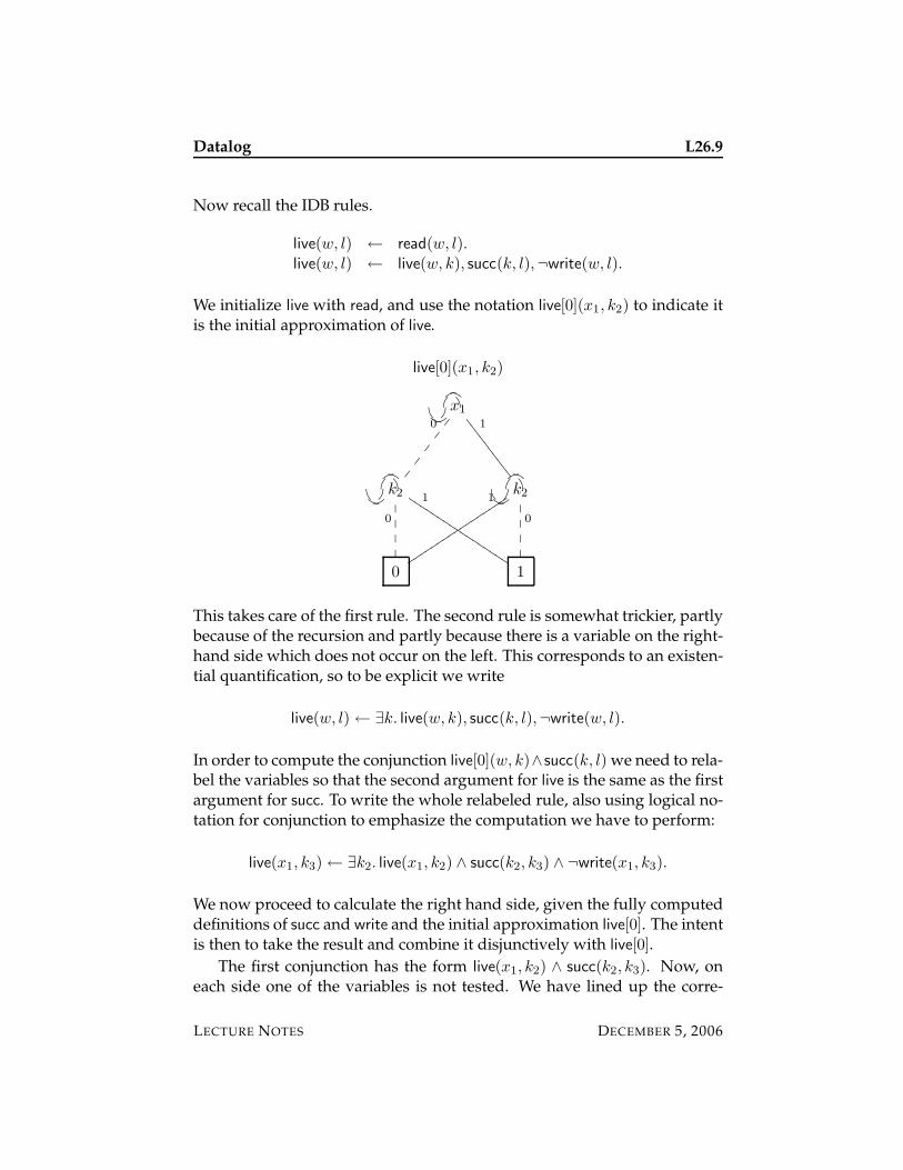
Datalog L26.9
Now recall the IDB rules.
live(w, l) ← read(w, l).live(w, l) ← live(w, k), succ(k, l),¬write(w, l).
We initialize live with read, and use the notation live[0](x1, k2) to indicate itis the initial approximation of live.
live[0](x1, k2)
GFED@ABC x1
0
��
��
� 1
8888
8888
88
GFED@ABC k2
0
���� 1
JJJJJJJJJJJJJJJJJGFED@ABC k2
1
ttttttttttttttttt
0
����
0 1
This takes care of the first rule. The second rule is somewhat trickier, partlybecause of the recursion and partly because there is a variable on the right-hand side which does not occur on the left. This corresponds to an existen-tial quantification, so to be explicit we write
live(w, l)← ∃k. live(w, k), succ(k, l),¬write(w, l).
In order to compute the conjunction live[0](w, k)∧succ(k, l) we need to rela-bel the variables so that the second argument for live is the same as the firstargument for succ. To write the whole relabeled rule, also using logical no-tation for conjunction to emphasize the computation we have to perform:
live(x1, k3)← ∃k2. live(x1, k2) ∧ succ(k2, k3) ∧ ¬write(x1, k3).
We now proceed to calculate the right hand side, given the fully computeddefinitions of succ and write and the initial approximation live[0]. The intentis then to take the result and combine it disjunctively with live[0].
The first conjunction has the form live(x1, k2) ∧ succ(k2, k3). Now, oneach side one of the variables is not tested. We have lined up the corre-
LECTURE NOTES DECEMBER 5, 2006
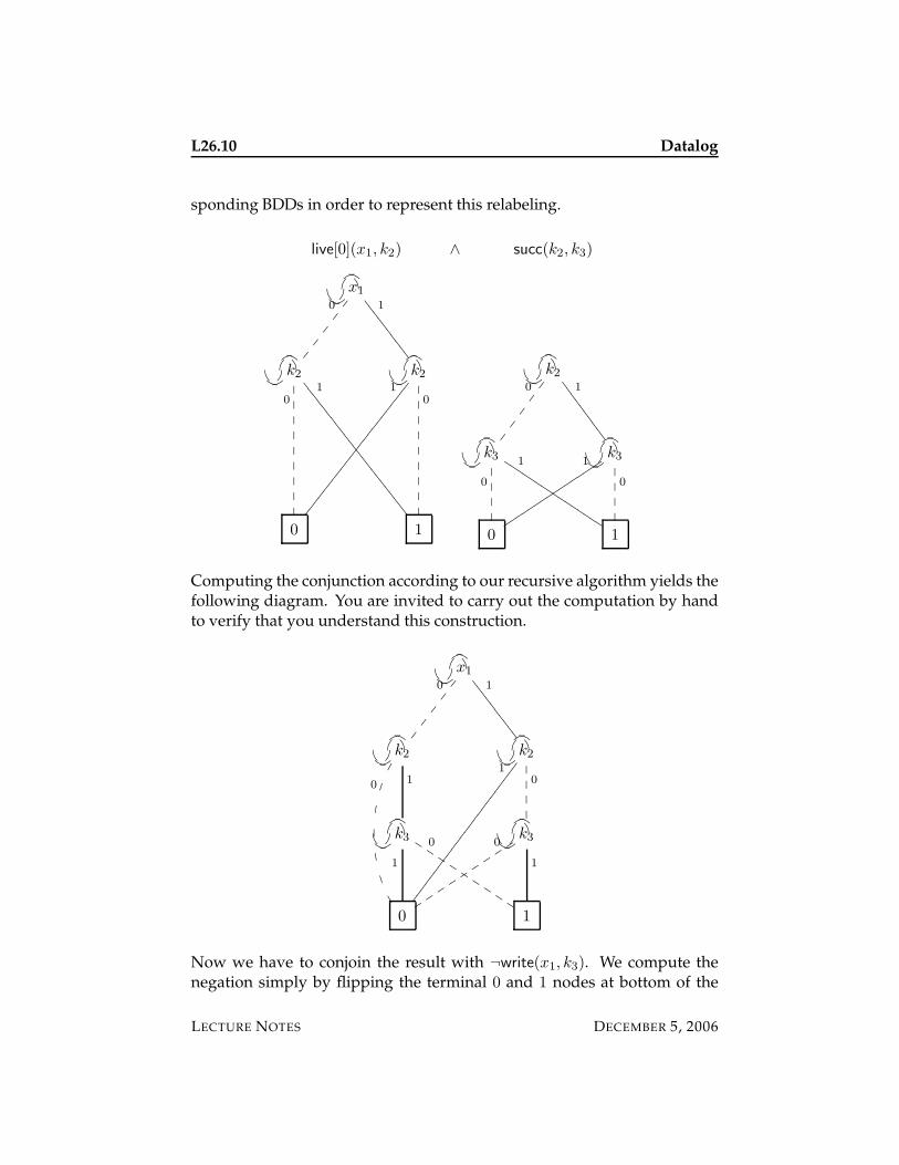
L26.10 Datalog
sponding BDDs in order to represent this relabeling.
live[0](x1, k2) ∧ succ(k2, k3)
GFED@ABC x1
0
��
��
� 1
8888
8888
88
GFED@ABC k2
0
���������
1
8888
8888
8888
8888
8888
888
GFED@ABC k2
1
����
����
����
����
����
���
0
���������
0 1
GFED@ABC k2
0
��
��
� 1
7777
7777
77
GFED@ABC k3
0
���� 1
JJJJJJJJJJJJJJJJGFED@ABC k3
1
tttttttttttttttt
0
����
0 1
Computing the conjunction according to our recursive algorithm yields thefollowing diagram. You are invited to carry out the computation by handto verify that you understand this construction.
GFED@ABC x1
0
��
��
� 1
8888
8888
88
GFED@ABC k2
0
�
��
$
)
1
1
GFED@ABC k2
1
����
����
����
����
����
����
0
����
GFED@ABC k3
1
0
JJ
JJJ
JJJ
JGFED@ABC k3
0
tt
tt t
tt
t t
1
0 1
Now we have to conjoin the result with ¬write(x1, k3). We compute thenegation simply by flipping the terminal 0 and 1 nodes at bottom of the
LECTURE NOTES DECEMBER 5, 2006
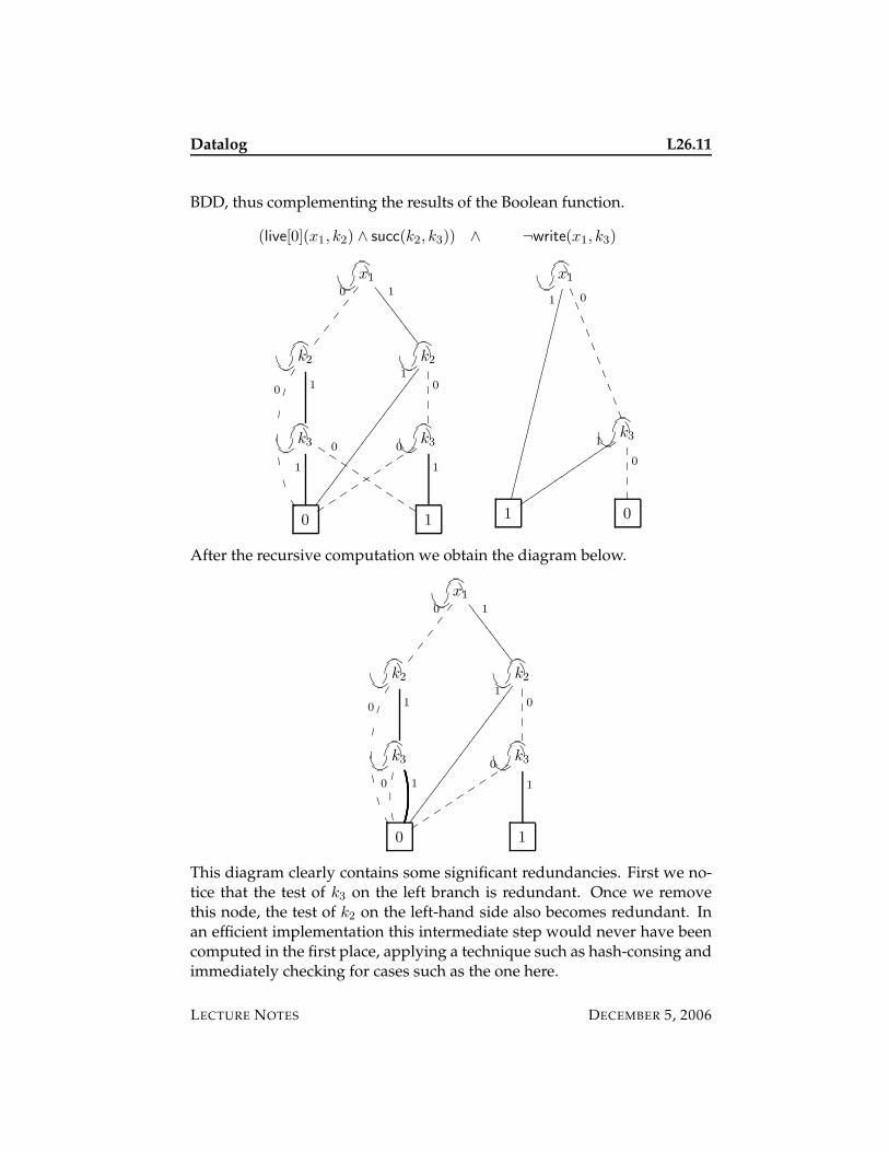
Datalog L26.11
BDD, thus complementing the results of the Boolean function.
(live[0](x1, k2) ∧ succ(k2, k3)) ∧ ¬write(x1, k3)
GFED@ABC x1
0
��
��
� 1
8888
8888
88
GFED@ABC k2
0
�
��
$
)
1
1
GFED@ABC k2
1
����
����
����
����
����
����
0
����
GFED@ABC k3
1
0
JJJ
JJ
JJJ
JGFED@ABC k3
0
tt
t tt
tt t
t
1
0 1
GFED@ABC x1
1
������������������������������ 0
,,
,,
,,
,,
,,
GFED@ABC k31
uuuuuuuuuuuuuuuu
0
����
1 0
After the recursive computation we obtain the diagram below.
GFED@ABC x1
0
��
��
� 1
8888
8888
88
GFED@ABC k2
0
�
��
$
)
1
1
GFED@ABC k2
1
����
����
����
����
����
����
0
����
GFED@ABC k3
0��
&
1
GFED@ABC k30
t tt
tt t
tt
t
1
0 1
This diagram clearly contains some significant redundancies. First we no-tice that the test of k3 on the left branch is redundant. Once we removethis node, the test of k2 on the left-hand side also becomes redundant. Inan efficient implementation this intermediate step would never have beencomputed in the first place, applying a technique such as hash-consing andimmediately checking for cases such as the one here.
LECTURE NOTES DECEMBER 5, 2006
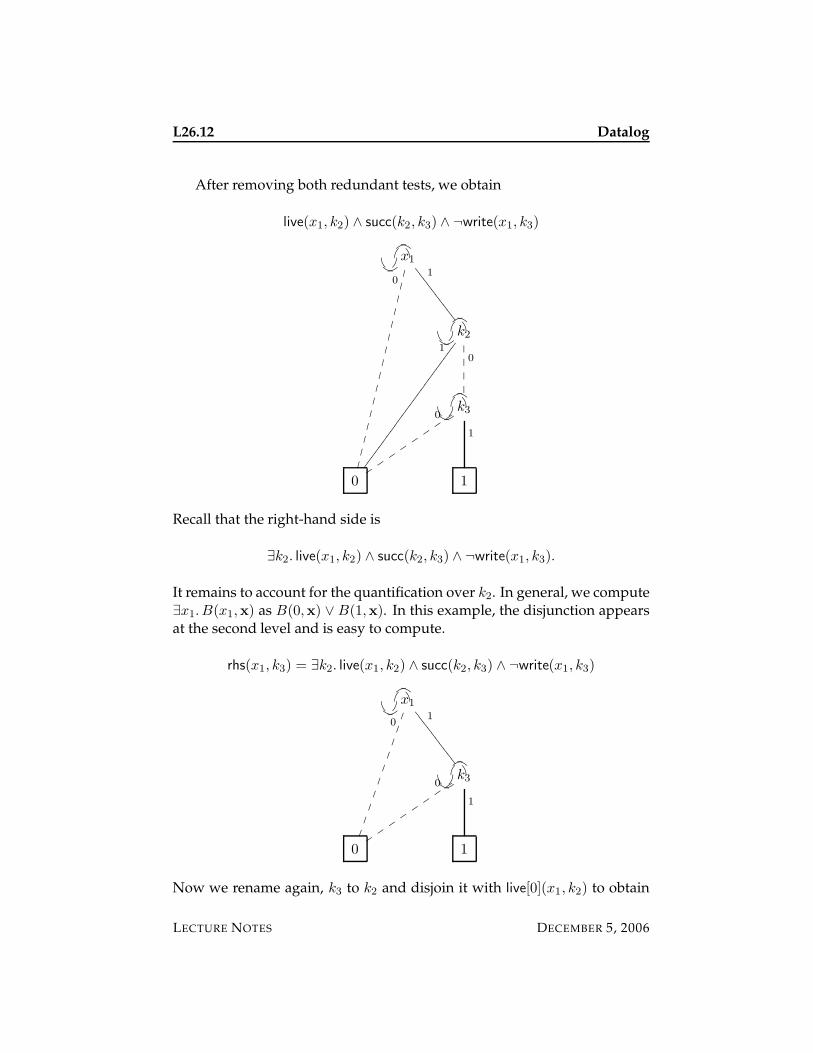
L26.12 Datalog
After removing both redundant tests, we obtain
live(x1, k2) ∧ succ(k2, k3) ∧ ¬write(x1, k3)
GFED@ABC x1
0
���������������� 1
8888
8888
88
GFED@ABC k2
1
����
����
����
����
����
����
0
����
GFED@ABC k30
uu
uu
uu
uu
1
0 1
Recall that the right-hand side is
∃k2. live(x1, k2) ∧ succ(k2, k3) ∧ ¬write(x1, k3).
It remains to account for the quantification over k2. In general, we compute∃x1. B(x1,x) as B(0,x) ∨ B(1,x). In this example, the disjunction appearsat the second level and is easy to compute.
rhs(x1, k3) = ∃k2. live(x1, k2) ∧ succ(k2, k3) ∧ ¬write(x1, k3)
GFED@ABC x1
0
���������� 1
8888
8888
88
GFED@ABC k30
uu
uu
uu
uu
1
0 1
Now we rename again, k3 to k2 and disjoin it with live[0](x1, k2) to obtain
LECTURE NOTES DECEMBER 5, 2006
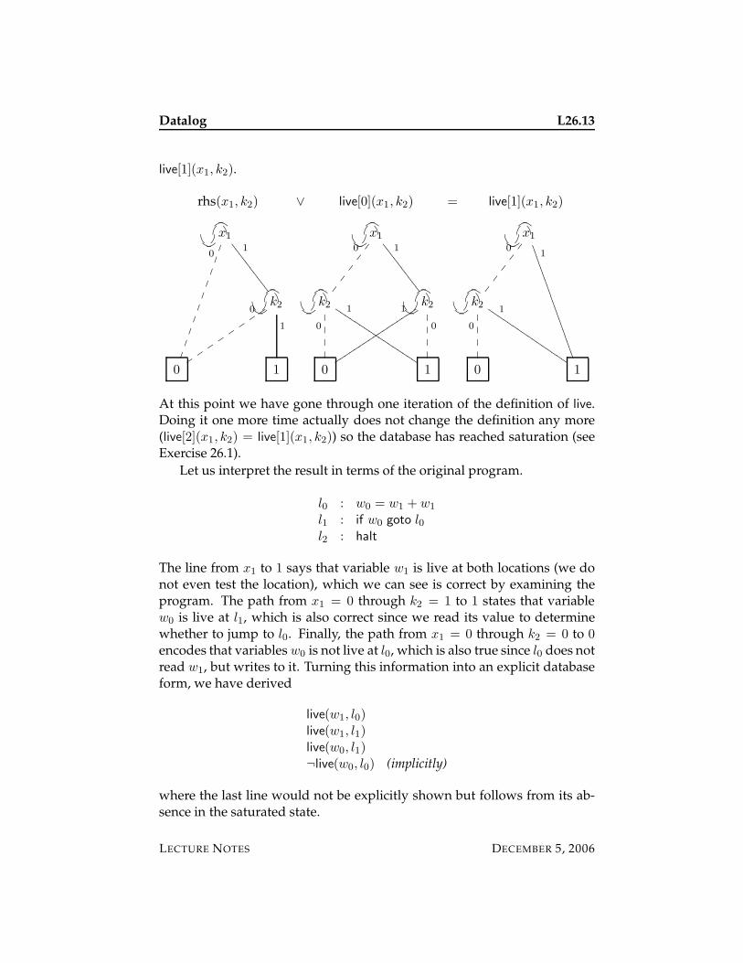
Datalog L26.13
live[1](x1, k2).
rhs(x1, k2) ∨ live[0](x1, k2) = live[1](x1, k2)
GFED@ABC x1
0
���������� 1
8888
8888
88
GFED@ABC k20
uu
uu
uu
uu
1
0 1
GFED@ABC x1
0
��
��
� 1
8888
8888
88
GFED@ABC k2
0
���� 1
JJJJJJJJJJJJJJJJJGFED@ABC k2
1
ttttttttttttttttt
0
����
0 1
GFED@ABC x1
0
��
��
�1
++++
++++
++++
++++
++++
GFED@ABC k2
0
���� 1
IIIIIIIIIIIIIIII
0 1
At this point we have gone through one iteration of the definition of live.Doing it one more time actually does not change the definition any more(live[2](x1, k2) = live[1](x1, k2)) so the database has reached saturation (seeExercise 26.1).
Let us interpret the result in terms of the original program.
l0 : w0 = w1 + w1
l1 : if w0 goto l0l2 : halt
The line from x1 to 1 says that variable w1 is live at both locations (we donot even test the location), which we can see is correct by examining theprogram. The path from x1 = 0 through k2 = 1 to 1 states that variablew0 is live at l1, which is also correct since we read its value to determinewhether to jump to l0. Finally, the path from x1 = 0 through k2 = 0 to 0encodes that variables w0 is not live at l0, which is also true since l0 does notread w1, but writes to it. Turning this information into an explicit databaseform, we have derived
live(w1, l0)live(w1, l1)live(w0, l1)¬live(w0, l0) (implicitly)
where the last line would not be explicitly shown but follows from its ab-sence in the saturated state.
LECTURE NOTES DECEMBER 5, 2006
L26.14 Datalog
While this may seem very tedious even in this small example, it has infact shown itself to be quite efficient even for very large programs. How-ever, a number of optimization are necessary to achieve this efficiency, asmentioned in the papers cited below.
26.7 Prospectus
BDDs were successfully employed in model checking for finite state sys-tems. In our setting, this would correspond to a linear forward chainingprocess where only the rules are unrestricted and facts are linear and thussubject to change on each iteration. Moreover, the states (represented aslinear contexts) would have to satisfy some additional invariants (for ex-ample, that each proposition occurs at most once in a context).
The research on Datalog has shown that we can use BDDs effectively forsaturating forward chaining computations. We believe this can be general-ized beyond Datalog if the forward chaining rules have a subterm propertyso that the whole search space remains finite. We only have to find a binarycoding of all terms in the search space so that the BDD representation tech-nique can be applied.
This strongly suggests that we could implement an interesting fragmentof LolliMon which would encompass both Datalog and some linear logicprograms subject to model checking, using BDDs as a uniform engine.
26.8 Historical Notes
The first use of deduction in databases is usually ascribed to a paper byGreen and Raphael [3] in 1968, which already employed a form of resolu-tion. The connection between logic programming, logic, and databases be-came firmly established during a workshop in Toulouse in 1977; selectedpapers were subsequently published in book form [2] which containedseveral seminal papers in logic programming. The name Datalog was notcoined until the 1980’s.
BDDs were first proposed by Randy Bryant [1]. Their use for imple-menting Datalog to statically analyze large programs was proposed andshown to be effective by John Whaley and collaborators [4], with a numberof more specialized and further papers we do not cite here. The resultingsystem, bddbddb (BDD-Based Deductive DataBase) is available on Source-Forge1.
1http://bddbddb.sourceforge.net/
LECTURE NOTES DECEMBER 5, 2006
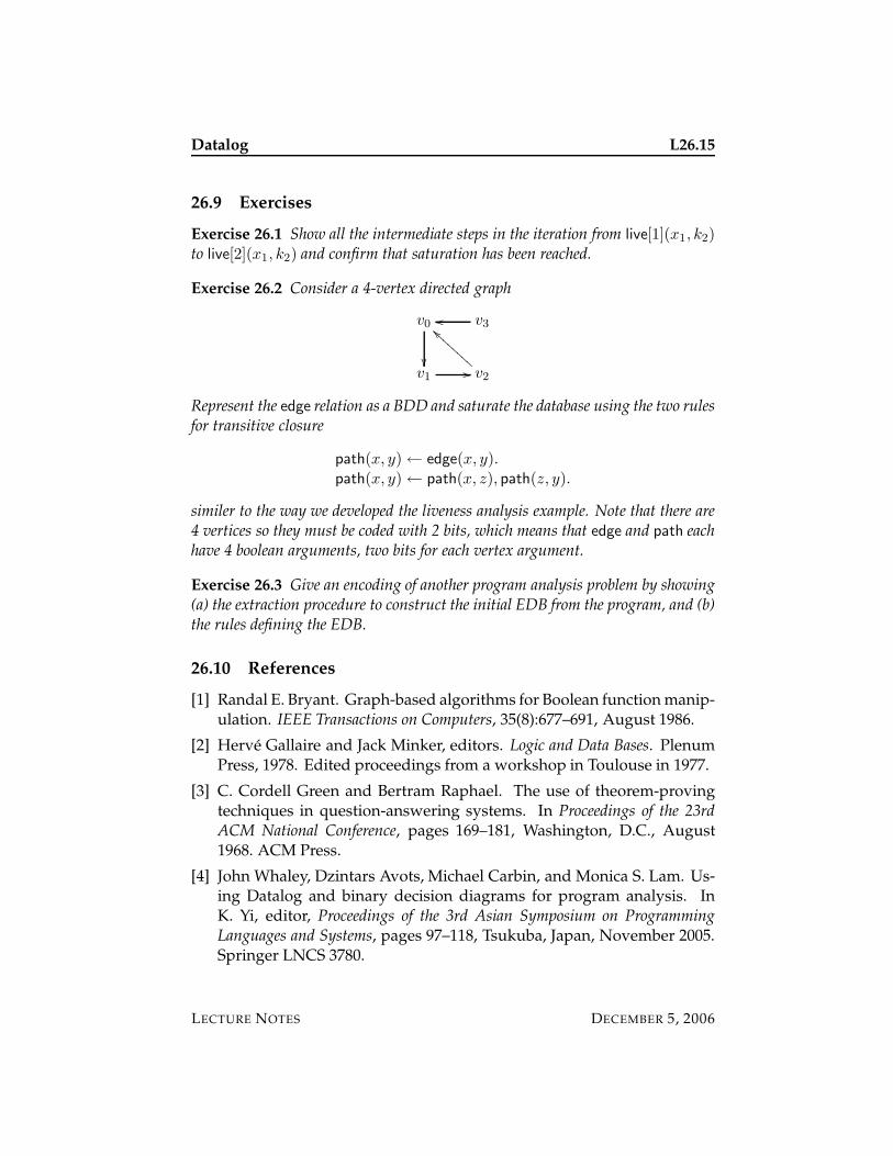
Datalog L26.15
26.9 Exercises
Exercise 26.1 Show all the intermediate steps in the iteration from live[1](x1, k2)to live[2](x1, k2) and confirm that saturation has been reached.
Exercise 26.2 Consider a 4-vertex directed graph
v0
��
v3oo
v1// v2
``BBBBBBBB
Represent the edge relation as a BDD and saturate the database using the two rulesfor transitive closure
path(x, y)← edge(x, y).path(x, y)← path(x, z), path(z, y).
similer to the way we developed the liveness analysis example. Note that there are4 vertices so they must be coded with 2 bits, which means that edge and path eachhave 4 boolean arguments, two bits for each vertex argument.
Exercise 26.3 Give an encoding of another program analysis problem by showing(a) the extraction procedure to construct the initial EDB from the program, and (b)the rules defining the EDB.
26.10 References
[1] Randal E. Bryant. Graph-based algorithms for Boolean function manip-ulation. IEEE Transactions on Computers, 35(8):677–691, August 1986.
[2] Herve Gallaire and Jack Minker, editors. Logic and Data Bases. PlenumPress, 1978. Edited proceedings from a workshop in Toulouse in 1977.
[3] C. Cordell Green and Bertram Raphael. The use of theorem-provingtechniques in question-answering systems. In Proceedings of the 23rdACM National Conference, pages 169–181, Washington, D.C., August1968. ACM Press.
[4] John Whaley, Dzintars Avots, Michael Carbin, and Monica S. Lam. Us-ing Datalog and binary decision diagrams for program analysis. InK. Yi, editor, Proceedings of the 3rd Asian Symposium on ProgrammingLanguages and Systems, pages 97–118, Tsukuba, Japan, November 2005.Springer LNCS 3780.
LECTURE NOTES DECEMBER 5, 2006

L26.16 Datalog
LECTURE NOTES DECEMBER 5, 2006
15-819K: Logic Programming
Lecture 27
Constraint Logic Programming
Frank Pfenning
December 7, 2006
In this lecture we sketch constraint logic programming which generalizesthe fixed structure of so-called uninterpreted function and predicate sym-bols of Horn logic. A common application is more flexible logic program-ming with arithmetic and finite domains. Higher-order logic programmingis another example where techniques from constraint logic programmingare important.
27.1 Arithmetic
One of the main motivations for constraint logic programming comes fromthe awkward and non-logical treatment of arithmetic in Prolog. For exam-ple, a naive implementation of the Fibonacci function would be the follow-ing Prolog program.
fib(0,1).
fib(1,1).
fib(N,F) :- N >= 2,
N1 is N-1, fib(N1,F1),
N2 is N-2, fib(N2,F2),
F is F1+F2.
Recall the use of is/2 to carry out evaluation of arithmetic predicates andthe built-in >=/2 to implement comparison between two ground terms.
Constraint logic programming supports interpreted function symbols(here: addition and subtraction) as term constructors, which means thatwe need to generalize unification to take into account the laws of arith-metic. Moreover, built-in predicates (here: comparison) over the constraint
LECTURE NOTES DECEMBER 7, 2006
L27.2 Constraint Logic Programming
domain (here: integers) are no longer restricted to ground terms but aretreated specially as part of the constraint domain.
In a constraint logic programming language over the integers, we couldrewrite the above program as
fib(0,1).
fib(1,1).
fib(N,F1+F2) :- N >= 2, fib(N-1,F1), fib(N-2,F2).
With respect to this program, a simple query
?- fib(2,F-1).
is perfectly legitimate and should yield F = 1, but even more complexqueries such as
?- N < 20, fib(N,5).
and
?- N < 20, fib(N,6).
will succeed (in first case, with N = 5) or fail finitely (in the second case).What emerges from the examples is that we need to extend ordinary
unification to handle more general equations, with terms from the con-straint domain, and that we furthermore need to generalize from just equal-ities to maintain other constraints such as inequalities.
27.2 An Operational Semantics with Constraints
Before we generalize to other domains, we return to the usual domain offirst-order terms and reformulate proof search. The idea is to replace unifi-cation by equality constraints.
We use the residuated form of programs in order to isolate the variouschoices and appeals to unification. Recall the language of goals G, goalstacks S and failure continuations F . We only consider the Horn fragment,so the program is fixed. Moreoever, we assume there is exactly one residu-ated program clause Dp for every predicate p.
Goals G ::= P | G1 ∧G2 | > | G1 ∨G2 | ⊥ | ∃x.G | s.= t
Programs D ::= ∀x. p(x)← G
Goal Stacks S ::= > | G ∧ S
Failure Conts. F ::= ⊥ | (G ∧ S) ∨ F
The operational semantics is given by three judgments.
LECTURE NOTES DECEMBER 7, 2006
Constraint Logic Programming L27.3
• G / S / F . Solve G under goal stack S with failure continuation F .
• s.= t | θ. Unification of s and t yields most general unifier θ.
• s.= t 6 |. Terms s and t are not unifiable.
We now add to this a constraint store C , for now just consisting of equa-tions.
Constraints C ::= > | s.= t ∧C
The first new judgment is
• G / S / C / F . Solve G under goal stack S and constraint C withfailure continuation F .
First, the rules for conjunction, which are not affected by the constraintexcept that they carry them along.
G1 / G2 ∧ S / C / F
G1 ∧G2 / S / C / F
G2 / S / C / F
> / G2 ∧ S / C / F > / > / C / F
We can see in the rule for final success that the constraint C represents aform of the answer. In practice, we project the constraints down to thevariables occurring in the original query, although we do not discuss thedetails of the projection operation in this lecture.
For disjunction we have to remember the constraint as well as the suc-cess continuation.
G1 / S / C / (G2 ∧ S ∧ C) ∨ F
G1 ∨G2 / S / C / F
G2 / S / C / F
⊥ / S′ / C ′ / (G2 ∧ S ∧ C) ∨ F
no rule for⊥ / S / C / ⊥
Predicate calls in residuated form do not involve unification, so theyremain unchanged from the unification-based semantics. Existential quan-tification is also straightforward.
(∀x. p(x)← G) ∈ Γ G(t/x) / S / C / F
p(t) / S / C / F
G(X/x) / S / C / F X 6∈ FV(S,C, F )
∃x.G / S / C / F
LECTURE NOTES DECEMBER 7, 2006
L27.4 Constraint Logic Programming
For equations, we no longer want to appeal to unification. Instead, wecheck if the new equation s
.= t together with the ones already present in C
are still consistent. If so, we add the new constraint s.= t; if not we fail and
backtrack.
s.= t ∧C 6` ⊥ > / S / s
.= t ∧ C / F
s.= t / S / C / F
s.= t ∧C ` ⊥ ⊥ / S / C / F
s.= t / S / C / F
We use a new judgment form, C ` ⊥, to check if a set of constraints isconsistent. It can be implemented simply by the left rules for equality, orby the forward chaining rules for unification described in an earlier lecture.The interpretation of variables, however, is a bit peculiar. The variables ina constraint C as part of the G / S / C / F are (implicitly) existentiallyquantified. When we ask if the constraints are inconsistent we mean tocheck that ¬∃X. C , that is, there does not exist a substitution t/X whichmakes C(t/X) true. We check this by assuming ∃X. C and trying to derivea contradiction. This means we introduce a new parameter x for each logicvariable X and actually try to prove C(x/X) where each of the variables x
is fresh. Since we are in the Horn fragment, we omitted this extra step ofback-substituting parameters since there is only one kind of variable.
An interesting point about the semantics above is that we no longer useor need substitutions θ. Whenever a new equation arrives we make sure thetotality of all equations encountered so far still has a solution and continue.
27.3 An Alternative Operational Semantics with Constraints
As noted, the treatment of variables in the above semantics is somewhatodd. We introduce them as logic variables, convert them to parameters tocheck consistency. But we never use them for anything else, so why intro-duce them as logic variables in the first place? Another jarring aspect of thesemantics is that the work that goes into determining that the equations areconsistent (for example, with the left rules for unifiability from an earlierlecture) is lost after the check, and we may have to redo a good bit of workwhen the next equality is encountered. In other words, the constraints arenot solved incrementally.
This suggests the following change in perspective: rather than trying toprove that there exists a unifying substitution, we think of search as tryingto characterize all unifying substitutions. We still need to treat the casethat there are none as special (so we can fail), but otherwise we just assumeconstraints. Reverting back to pure logic for a moment, a sequent C ` A
LECTURE NOTES DECEMBER 7, 2006
Constraint Logic Programming L27.5
with parameters x holds if any substitution t/x which makes C true alsomakes A true.
Once constraints appear on the left-hand side, they can be treated withthe usual left rules. The main judgment is now C ` G / S / F for a set ofconstraints C where we maintain the invariant that C is always satisfiable(that is, it is never the case that C ` ⊥). This should be parenthesized as(C ` G / S) / F because the constraints C do not apply to F .
For most of the rules from above this is a mere notational change. Wea few interesting cases. We generalize the left-hand side slightly to be acollection of constraints C instead of a single one.
C ` G1 / S / (C ` G2 ∧ S) ∨ F
C ` G1 ∨G2 / S / F
C ` G2 / S / F
C′ ` ⊥ / S′ / (C ` G2 ∧ S) ∨ F
no rule forC ` ⊥ / S / ⊥
Existential quantification now introduces a new parameter.
C ` G / S / F x 6∈ FV(S, C, F )
C ` ∃x.G / S / F
We avoid the issue of types and a typed context of parameters as we dis-cussed in the lecture of parameters.
Equality is now treated differently.
C, s.= t 6` ⊥ C, s
.= t ` > / S / F
C ` s.= t / S / F
C, s.= t ` ⊥ C ` ⊥ / S / F
C ` s.= t / S / F
Now there is scope for various left rules concerning equality. The sim-plest example is the left rule for equality discussed in an earlier lecture.This actually recovers the usual unification semantics!
s.= t | θ (Cθ ` Gθ / Sθ) / F
(C, s.= t ` G / S) / F
Note that the other case of the left rule (where s and t do not have a unifier)cannot arise because of our satisfiability invariant which guarantees that aunifier exists.
We can also use the small-step rules dealing with equality that willnever apply a substitution, just accumulate information about the vari-ables. For example, knowing x
.= c for a constant c carries the same in-
formation as applying the substitution c/x.
LECTURE NOTES DECEMBER 7, 2006
L27.6 Constraint Logic Programming
These left rules will put a satisfiable constraint into a kind of reducedform and in practice this is combined with the satisfiability check. Thismeans constraints are treated incrementally, which is of great practical im-portance especially in complex constraint domains.
As a final remark, we come back to focusing. The rules for equalitycreate a kind of non-determinism, because either we could solve a goal orwe could break down the equality we just assumed. However, the rules forequality are asynchronous on the left and can be reduced eagerly until weget irreducible equations. In a complete, lower-level semantics this shouldbe addressed explicitly; we omit this step here and leave it as Exercise 27.1.
27.4 Richer Constraint Domains
The generalization to richer domains is now not difficult. Instead of justequalities, the constraint C (or the constraint collection C) contains otherinterpreted predicate symbols such as inequalities of even disequalities.When encountering an equality or interpreted predicate we verify its con-sistency, adding it to the set of constraints.
In addition we allow either constraint simplification, or saturate leftrules for the predicates in the constraint domain. The simplification al-gorithms depend significantly on the particular constraint domains. Forexample, for arithmetic equalities we might use Gaussian elimination, forarithmetic inequalities the simplex algorithm. In addition we need to con-sider combinations of constraint domains, for which there are general ar-chitectures such as the Nelson-Oppen method for combining decision pro-cedures.
A particularly popular constraint domain is Finite Domains (FD), whichis supported in implementations such as GNU Prolog. This also supportsbounded arithmetic as a special case. We will not go into further detail,except to say that the Fibonacci example is expressible in several constraintlanguages.
27.5 Hard Constraints
An important concept in practical constraint domains is that of a hard con-straint. Hard constraints may be difficult to solve, or may even be unde-cidable. The general strategy in constraint programming language is topostpone the solution of hard constraints until further instantiations makethem tractable. An example might be
?- X * Y = 4, X = 2.
LECTURE NOTES DECEMBER 7, 2006
Constraint Logic Programming L27.7
When we see X * Y = 4, the equation is non-linear, so we would be justi-fied in raising an exception if the domain was supposed to treat only linearequations. But when we receive the second constraint, X = 2, we can sim-plify the first constraint to be linear 2 * Y = 4 and simplify to Y = 2.
When hard constraints are left after overall “success”, the success mustbe interpreted conditionally: any solution to the remaining hard constraintsyields a solution to the overall query. It is even possible that the hard con-straints may have no solution, negating an apparent success, so extra caremust be taken when the interpreter admits hard constraints.
Hard constraints arise naturally in arithmetic. Another domain wherehard constraints play a significant role is that of terms containing abstrac-tions (higher-order abstract syntax), where constraint solving is a form ofhigher-order unification. This is employed, for example, in the Twelf sys-tems, where hard constraints (those falling outside the pattern fragment)are postponed and reawakened when more information may make themtractable.
27.6 Detailed Example
As our example we consider the Fibonacci sequence again.
fib(0,1).
fib(1,1).
fib(N,F1+F2) :- N >= 2, fib(N-1,F1), fib(N-2,F2).
We use it in this direct form, rather then the residuated form for brevity. Weconsider the query
?- N < 10, fib(N,2).
which inverts the Fibonacci functions, asking for which n < 10 we havefib(n) = 2. The bound on n is to avoid possible non-termination, althoughhere it would only affect search after the first solution. Inverting the Fi-bonacci function directly as with this query is impossible with ordinaryProlog programs.
Below we show G / S / C , omitting the failure continuation andsilently simplifying constraints on occasion. We avoid redundant “ ∧ >”and use Prolog notation throughout. Furthermore, we have substituted forthe first occurrence of a variable in a clause head instead of building anequality constraint.
LECTURE NOTES DECEMBER 7, 2006
L27.8 Constraint Logic Programming
N < 10, fibr(N,2) / true / true
fib(N,2) / true / N < 10
% trying clause fib(0,1)
% 0 = N , 1 = 2, N < 10 is inconsistent
% trying clause fib(1,1)
% 1 = N , 1 = 2, N < 10 is inconsistent
% trying clause fib(N,F1+F2) :- ...
F1+F2 = 2 / N >= 2, fib(N-1,F1), fib(N-2,F2) / N < 10
N >= 2 / fib(N-1,F1), fib(N-2,F2) / F1 = 2-F2, N < 10
fib(N-1,F1) / fib(N-2,F2) / F1 = 2-F2, 2 <= N, N < 10
% trying clause fib(0,1)
% 0 = N-1, 1 = F1, F1 = 2-F2, 2 <= N, N < 10 is incons.
% trying clause fib(1,1)
1 = N-1, 1 = F1 / fib(N-2,F2) / F1 = 2-F2, 2 <= N, N < 10
fib(N-2,F2) / true / F1 = 2-F2, N = 2
% trying clause fib(0,1)
0 = N-2, 1 = F2 / true / F1 = 2-F2, N = 2
true / true / 0 = N-2, 1 = F2, F1 = 2-F2, N = 2
true / true / N = 2, F2 = 1, F1 = 1
Even though GNU Prolog offers finite domain constraints, includinginteger ranges, the Fibonacci program above does not quite run as given.The problem is that, in order to be backward compatible with Prolog, thepredicates of the constraint domain (including equality) must be separatedout. The naming convention is to precede a predicate with # to obtain thecorresponding constraint predicate (assuming it is defined). Here is a bi-directional version of the Fibonacci predicate in GNU Prolog.
fibc(0,1).
fibc(1,1).
fibc(N,F) :- N #>= 2,
N1 #= N-1, fibc(N1,F1),
N2 #= N-2, fibc(N2,F2),
F #= F1+F2.
With this predicate we can execute queries such as
?- N #< 10, fibc(N,8).
(which succeeds) and
?- N #< 10, fibc(N,9).
LECTURE NOTES DECEMBER 7, 2006
Constraint Logic Programming L27.9
(which fails). A query
?- N < 10, fibc(N,8).
would signal an error, because the first argument to < is not ground.
27.7 Historical Notes
Constraint logic programming was first proposed by Jaffar and Lassez [3].The first practical implementation was by Jaffar and Michaylov [4], the fullCLP(R) language and system later described by Jaffar et al. [5]. A relatedlanguage is Prolog III [1] which combines several constraint domains. Theview of higher-order logic programming as constraint logic programmingwas advanced by Michaylov and myself [8, 6].
The architecture of cooperating decision procedures is due to Nelsonand Oppen [7].
In the above constraint logic programming language the constraintsand their solution algorithms are hard-wired into the language. The sub-language of Constraint Handling Rules (CHR) [2] aims at allowing thespecification of constraint simplification within the language for greaterflexibility. It seems that this is a fragment of LolliMon, specifically, its linearforward chaining sublanguage, which could be the basis for a more logicalexplanation of constraints and constraint simplification in logic program-ming.
27.8 Exercises
Exercise 27.1 Write a semantics for Horn logic where unification is replaced byincremental constraint solving as sketched in this lecture. Make sure your ruleshave no unwanted non-determinism, that is, they can be viewed as a deterministicabstract machine.
27.9 References
[1] Alain Colmerauer. An introduction to Prolog III. Communications of theACM, 33(7):69–90, 1990.
[2] Thom Fruwirth. Theory and practice of constraint handling rules. Jour-nal of Logic Programming, 17(1–3):95–138, October 1998.
[3] Joxan Jaffar and Jean-Louis Lassez. Constraint logic programming. InProceedings of the 14th Annual Symposium on Principles of ProgrammingLanguages, pages 111–119, Munich, Germany, January 1987. ACM Press.
LECTURE NOTES DECEMBER 7, 2006
L27.10 Constraint Logic Programming
[4] Joxan Jaffar and Spiro Michaylov. Methodology and implementation ofa CLP system. In J.-L. Lassez, editor, Proceedings of the 4th InternationalConference on Logic Programming (ICLP’87), pages 196–218, Melbourne,Australia, May 1987. MIT Press.
[5] Joxan Jaffar, Spiro Michaylov, Peter J. Stuckey, and Roland H. C. Yap.The CLP(R) language and system. ACM Transactions on ProgrammingLanguages and Systems, 14(3):339–395, July 1992.
[6] Spiro Michaylov and Frank Pfenning. Higher-order logic program-ming as constraint logic programming. In Position Papers for the FirstWorkshop on Principles and Practice of Constraint Programming, pages 221–229, Newport, Rhode Island, April 1993. Brown University.
[7] Greg Nelson and Derek C. Oppen. Simplification by cooperating deci-sion procedures. ACM Transactions on Programming Languages and Sys-tems, 1(2):245–257, 1979.
[8] Frank Pfenning. Logic programming in the LF logical framework. InGerard Huet and Gordon Plotkin, editors, Logical Frameworks, pages149–181. Cambridge University Press, 1991.
LECTURE NOTES DECEMBER 7, 2006