logic and proof - university of · pdf file · 2002-09-13i logic and proof 1 slide...
TRANSCRIPT

Logic and Proof
Computer Science Tripos Part IBMichaelmas Term
Lawrence C Paulson
Computer Laboratory
University of Cambridge
Copyright c© 2002 by Lawrence C. Paulson

Contents
1 Introduction 1
2 Propositional Logic 6
3 Gentzen’s Logical Calculi 11
4 Ordered Binary Decision Diagrams 16
5 First-Order Logic 21
6 Formal Reasoning in First-Order Logic 26
7 Davis-Putnam & Propositional Resolution 31
8 Skolem Functions and Herbrand’s Theorem 36
9 Unification 41
10 Resolution and Prolog 46
11 Modal Logics 51
12 Tableaux-Based Methods 56

I Logic and Proof 1
Slide 101
Introduction to Logic
Logic concerns statements in some language
The language can be informal (e.g. English) or formal
Some statements are true, others false or perhaps meaningless, . . .
Logic concerns relationships between statements: consistency,
entailment, . . .
Logical proofs model human reasoning
Slide 102
Statements
Statements are declarative assertions:
Black is the colour of my true love’s hair.
They are not greetings, questions, commands, . . .:
What is the colour of my true love’s hair?
I wish my true love had hair.
Get a haircut!

I Logic and Proof 2
Slide 103
Schematic Statements
The meta-variables X, Y, Z, . . . range over ‘real’ objects
Black is the colour of X’s hair.
Black is the colour of Y.
Z is the colour of Y.
Schematic statements can express general statements, or questions:
What things are black?
Slide 104
Interpretations and Validity
An interpretation maps meta-variables to real objects
The interpretation Y 7→ coal satisfies the statement
Black is the colour of Y.
but the interpretation Y 7→ strawberries does not!
A statement A is valid if all interpretations satisfy A.

I Logic and Proof 3
Slide 105
Consistency, or Satisfiability
A set S of statements is consistent if some interpretation satisfies all
elements of S at the same time. Otherwise S is inconsistent.
Examples of inconsistent sets:
{X part of Y, Y part of Z, X NOT part of Z}
{n is a positive integer, n 6= 1, n 6= 2, . . .}
satisfiable/unsatisfiable = consistent/inconsistent
Slide 106
Entailment, or Logical Consequence
A set S of statements entails A if every interpretation that satisfies all
elements of S, also satisfies A. We write S |= A.
{X part of Y, Y part of Z} |= X part of Z
{n 6= 1, n 6= 2, . . .} |= n is NOT a positive integer
S |= A if and only if {¬A} ∪ S is inconsistent
|= A if and only if A is valid

I Logic and Proof 4
Slide 107
Inference
Want to check A is valid
Checking all interpretations can be effective — but if there are
infinitely many?
Let {A1, . . . , An} |= B. If A1, . . ., An are true then B must be
true. Write this as the inference
A1 . . . An
B
Use inferences to construct finite proofs!
Slide 108
Schematic Inference Rules
X part of Y Y part of Z
X part of Z
A valid inference:
spoke part of wheel wheel part of bike
spoke part of bike
An inference may be valid even if the premises are false!
cow part of chair chair part of ant
cow part of ant

I Logic and Proof 5
Slide 109
Survey of Formal Logics
propositional logic is traditional boolean algebra.
first-order logic can say for all and there exists.
higher-order logic reasons about sets and functions. It has been
applied to hardware verification.
modal/temporal logics reason about what must, or may, happen.
type theories support constructive mathematics.
Slide 110
Why Should the Language be Formal?
Consider this ‘definition’:
The least integer not definable using eight words
Greater than The number of atoms in the entire Universe
Also greater than The least integer not definable using eight words
• A formal language prevents AMBIGUITY.

II Logic and Proof 6
Slide 201
Syntax of Propositional Logic
P, Q, R, . . . propositional letter
t true
f false
¬A not A
A ∧ B A and B
A ∨ B A or B
A → B if A then B
A ↔ B A if and only if B
Slide 202
Semantics of Propositional Logic
¬, ∧, ∨, → and↔ are truth-functional: functions of their operands
A B ¬A A ∧ B A ∨ B A → B A ↔ B
t t f t t t t
t f f f t f f
f t t f t t f
f f t f f t t

II Logic and Proof 7
Slide 203
Interpretations of Propositional Logic
An interpretation is a function from the propositional letters to {t, f }.
Interpretation I satisfies a formula A if the formula evaluates to t.
Write |=I A
A is valid (a tautology ) if every interpretation satisfies A
Write |= A
S is satisfiable if some interpretation satisfies every formula in S
Slide 204
Implication, Entailment, Equivalence
A → B means simply ¬A ∨ B
A |= B means if |=I A then |=I B for every interpretation I
A |= B if and only if |= A → B
Equivalence
A ' B means A |= B and B |= A
A ' B if and only if |= A ↔ B

II Logic and Proof 8
Slide 205
Equivalences
A ∧A ' A
A ∧ B ' B ∧A
(A ∧ B) ∧ C ' A ∧ (B ∧ C)
A ∨ (B ∧ C) ' (A ∨ B) ∧ (A ∨ C)
A ∧ f ' f
A ∧ t ' A
A ∧ ¬A ' f
Dual versions: exchange ∧, ∨ and t, f in any equivalence
Slide 206
Negation Normal Form
1. Get rid of ↔ and→, leaving just ∧, ∨, ¬:
A ↔ B ' (A → B) ∧ (B → A)
A → B ' ¬A ∨ B
2. Push negations in, using de Morgan’s laws:
¬¬A ' A
¬(A ∧ B) ' ¬A ∨ ¬B
¬(A ∨ B) ' ¬A ∧ ¬B

II Logic and Proof 9
Slide 207
From NNF to Conjunctive Normal Form
3. Push disjunctions in, using distributive laws:
A ∨ (B ∧ C) ' (A ∨ B) ∧ (A ∨ C)
(B ∧ C) ∨A ' (B ∨A) ∧ (C ∨A)
4. Simplify:
• Delete any disjunction containing P and ¬P
• Delete any disjunction that includes another
• Replace (P ∨A) ∧ (¬P ∨A) by A
Slide 208
Converting a Non-Tautology to CNF
P ∨Q → Q ∨ R
1. Elim →: ¬(P ∨Q) ∨ (Q ∨ R)
2. Push ¬ in: (¬P ∧ ¬Q) ∨ (Q ∨ R)
3. Push ∨ in: (¬P ∨Q ∨ R) ∧ (¬Q ∨Q ∨ R)
4. Simplify: ¬P ∨Q ∨ R
Not a tautology: try P 7→ t, Q 7→ f , R 7→ f

II Logic and Proof 10
Slide 209
Tautology checking using CNF
((P → Q) → P) → P
1. Elim →: ¬[¬(¬P ∨Q) ∨ P] ∨ P
2. Push ¬ in: [¬¬(¬P ∨Q) ∧ ¬P] ∨ P
[(¬P ∨Q) ∧ ¬P] ∨ P
3. Push ∨ in: (¬P ∨Q ∨ P) ∧ (¬P ∨ P)
4. Simplify: t ∧ t
t It’s a tautology!

III Logic and Proof 11
Slide 301
A Simple Proof System
Axiom Schemes
K A → (B → A)
S (A → (B → C)) → ((A → B) → (A → C))
DN ¬¬A → A
Inference Rule: Modus Ponens
A → B AB
Slide 302
A Simple (?) Proof of A → A
(A → ((D → A) → A)) → (1)
((A → (D → A)) → (A → A)) by S
A → ((D → A) → A) by K (2)
(A → (D → A)) → (A → A) by MP, (1), (2) (3)
A → (D → A) by K (4)
A → A by MP, (3), (4) (5)

III Logic and Proof 12
Slide 303
Some Facts about Deducibility
A is deducible from the set S of if there is a finite proof of A starting
from elements of S. Write S ` A.
Soundness Theorem. If S ` A then S |= A.
Completeness Theorem. If S |= A then S ` A.
Deduction Theorem. If S ∪ {A} ` B then S ` A → B.
Slide 304
Gentzen’s Natural Deduction Systems
A varying context of assumptions
Each logical connective defined independently
Introduction rule for ∧: how to deduce A ∧ B
A BA ∧ B
Elimination rules for ∧: what to deduce from A ∧ B
A ∧ BA
A ∧ BB

III Logic and Proof 13
Slide 305
The Sequent Calculus
Sequent A1, . . . , Am⇒B1, . . . , Bn means,
if A1 ∧ . . . ∧Am then B1 ∨ . . . ∨ Bn
A1, . . ., Am are assumptions; B1, . . ., Bn are goals
Γ and ∆ are sets in Γ⇒∆
A, Γ⇒A, ∆ is trivially true (basic sequent)
Slide 306
Sequent Calculus Rules
Γ⇒∆, A A, Γ⇒∆
Γ⇒∆(cut)
Γ⇒∆, A
¬A, Γ⇒∆(¬l)
A, Γ⇒∆
Γ⇒∆, ¬A(¬r)
A, B, Γ⇒∆
A ∧ B, Γ⇒∆(∧l)
Γ⇒∆, A Γ⇒∆, B
Γ⇒∆, A ∧ B(∧r)

III Logic and Proof 14
Slide 307
More Sequent Calculus Rules
A, Γ⇒∆ B, Γ⇒∆
A ∨ B, Γ⇒∆(∨l)
Γ⇒∆, A, B
Γ⇒∆, A ∨ B(∨r)
Γ⇒∆, A B, Γ⇒∆
A → B, Γ⇒∆(→l)
A, Γ⇒∆, B
Γ⇒∆, A → B(→r)
Slide 308
Easy Sequent Calculus Proofs
A, B⇒A
A ∧ B⇒A(∧l)
⇒A ∧ B → A(→r)
A, B⇒B, A
A⇒B, B → A(→r)
⇒A → B, B → A(→r)
⇒ (A → B) ∨ (B → A)(∨r)

III Logic and Proof 15
Slide 309
Part of a Distributive Law
A⇒A, B
B, C⇒A, B
B ∧ C⇒A, B(∧l)
A ∨ (B ∧ C)⇒A, B(∨l)
A ∨ (B ∧ C)⇒A ∨ B(∨r)
similar
A ∨ (B ∧ C)⇒ (A ∨ B) ∧ (A ∨ C)(∧r)
Second subtree proves A ∨ (B ∧ C)⇒A ∨ C similarly
Slide 310
A Failed Proof
A⇒B, C B⇒B, C
A ∨ B⇒B, C(∨l)
A ∨ B⇒B ∨ C(∨r)
⇒A ∨ B → B ∨ C(→r)
A 7→ t, B 7→ f , C 7→ f falsifies unproved sequent!

IV Logic and Proof 16
Slide 401
Ordered Binary Decision Diagrams
Canonical form: essentially decision trees with sharing
• ordered propositional symbols (‘variables’)
• sharing of identical subtrees
• hashing and other optimisations
Detects if a formula is tautologous (t) or inconsistent (f )
A FAST way of verifying digital circuits, . . .
Slide 402
Decision Diagram for (P ∨Q) ∧ R
P
Q
R R
1000 0 01 1
Q
R R

IV Logic and Proof 17
Slide 403
Converting a Decision Diagram to an OBDD
P
Q
R
Q
R
0 1
P
Q
R
0 1
No duplicates No redundant tests
Slide 404
Building OBDDs Efficiently
Do not construct full tree! (see Bryant, §3.1)
Do not expand→, ↔, ⊕ (exclusive OR) to other connectives
Treat ¬Z as Z → f or Z⊕ t
Recursively convert operands
Combine operand OBDDs — respecting ordering and sharing
Delete test if it proves to be redundant

IV Logic and Proof 18
Slide 405
Canonical Form Algorithm
To do Z ∧ Z ′, where Z and Z ′ are already canonical:
Trivial if either is t or f . Treat ∨, →, ↔ similarly!
Let Z = if(P, X, Y) and Z ′ = if(P ′, X ′, Y ′)
If P = P ′ then recursively do if(P, X ∧ X ′, Y ∧ Y ′)
If P < P ′ then recursively do if (P, X ∧ Z ′, Y ∧ Z ′)
If P > P ′ then recursively do if (P ′, Z ∧ X ′, Z ∧ Y ′)
Slide 406
Canonical Form of P ∨Q
P
0 1
Q
0 1
P
∨

IV Logic and Proof 19
Slide 407
Canonical Form of P ∨Q → Q ∨ R
Q
0 1
P →
R
0 1
Q
Q
P
R
0 1
Q
P
Slide 408
Optimisations Based On Hash Tables
Never build the same OBDD twice: share pointers
• Pointer identity: X = Y whenever X ↔ Y
• Fast removal of redundant tests by if(P, X, X) ' X
• Fast processing of X ∧ X, X ∨ X, X → X, . . .
Never process X ∧ Y twice; keep table of canonical forms

IV Logic and Proof 20
Slide 409
Final Observations
The variable ordering is crucial. Consider
(P1 ∧Q1) ∨ · · · ∨ (Pn ∧Qn)
A good ordering is P1 < Q1 < · · · < Pn < Qn
A dreadful ordering is P1 < · · · < Pn < Q1 < · · · < Qn
Many digital circuits have small OBDDs (not multiplication!)
OBDDs can solve problems in hundreds of variables
General case remains intractable!
V Logic and Proof 21
Slide 501
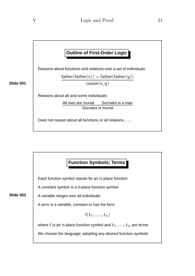
Outline of First-Order Logic
Reasons about functions and relations over a set of individuals
father(father(x)) = father(father(y))
cousin(x, y)
Reasons about all and some individuals:
All men are mortal Socrates is a manSocrates is mortal
Does not reason about all functions or all relations, . . .
Slide 502
Function Symbols; Terms
Each function symbol stands for an n-place function
A constant symbol is a 0-place function symbol
A variable ranges over all individuals
A term is a variable, constant or has the form
f(t1, . . . , tn)
where f is an n-place function symbol and t1, . . ., tn are terms
We choose the language, adopting any desired function symbols
V Logic and Proof 22
Slide 503
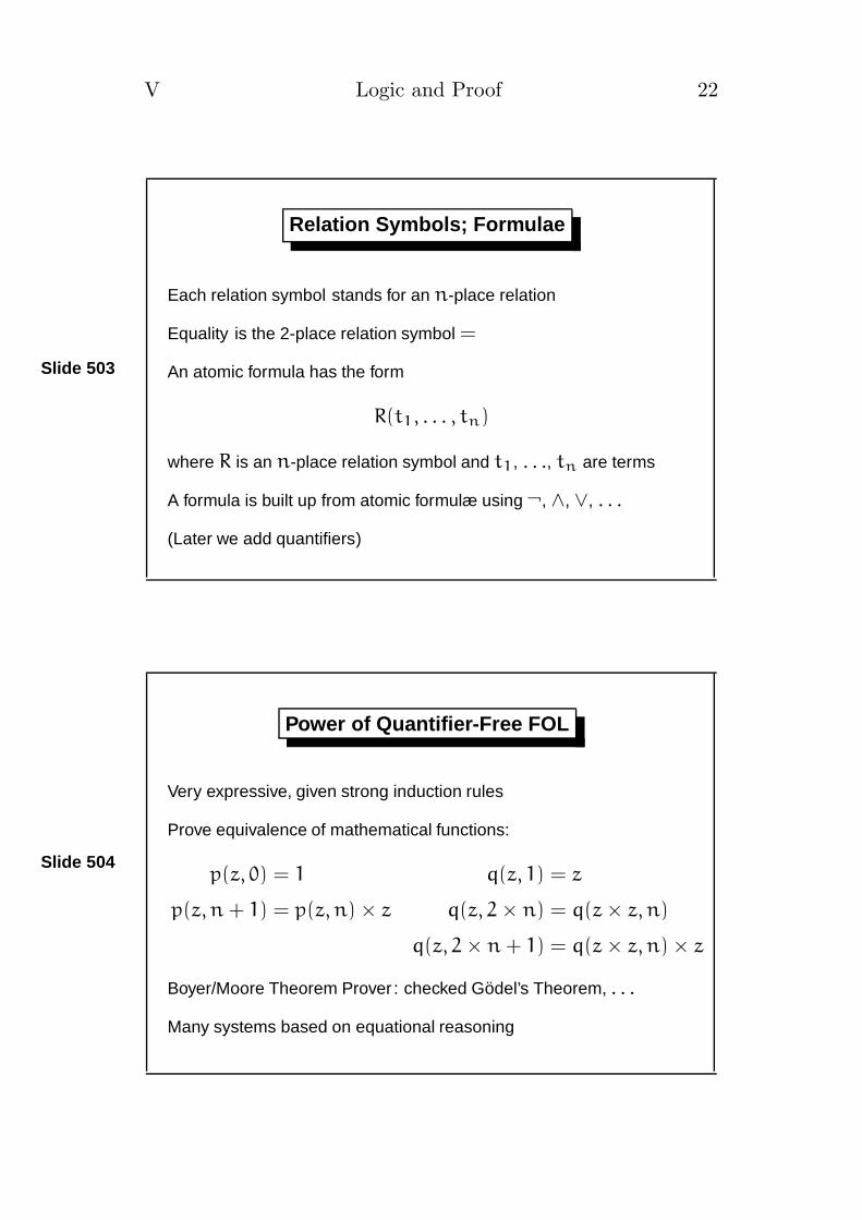
Relation Symbols; Formulae
Each relation symbol stands for an n-place relation
Equality is the 2-place relation symbol =
An atomic formula has the form
R(t1, . . . , tn)
where R is an n-place relation symbol and t1, . . ., tn are terms
A formula is built up from atomic formulæ using ¬, ∧, ∨, . . .
(Later we add quantifiers)
Slide 504
Power of Quantifier-Free FOL
Very expressive, given strong induction rules
Prove equivalence of mathematical functions:
p(z, 0) = 1
p(z, n + 1) = p(z, n) × z
q(z, 1) = z
q(z, 2× n) = q(z× z, n)
q(z, 2× n + 1) = q(z× z, n) × z
Boyer/Moore Theorem Prover : checked Godel’s Theorem, . . .
Many systems based on equational reasoning

V Logic and Proof 23
Slide 505
Universal and Existential Quantifiers
∀x A for all x, A holds
∃x A there exists x such that A holds
Syntactic variations:
∀xyz A abbreviates ∀x ∀y ∀z A
∀z . A ∧ B is an alternative to ∀z (A ∧ B)
The variable x is bound in ∀x A; compare with∫
f(x)dx
Slide 506
Expressiveness of Quantifiers
All men are mortal:
∀x (man(x) → mortal(x))
All mothers are female:
∀x female(mother(x))
There exists a unique x such that A, written ∃!x A
∃x [A(x) ∧ ∀y (A(y) → y = x)]

V Logic and Proof 24
Slide 507
How do we interpret mortal(Socrates)?
Interpretation I = (D, I) of our first-order language
D is a non-empty universe
I maps symbols to ‘real’ functions, relations
c a constant symbol I[c] ∈ D
f an n-place function symbol I[f] ∈ Dn → D
P an n-place relation symbol I[P] ⊆ Dn
Slide 508
How do we interpret cousin(Charles, y)?
A valuation supplies the values of free variables
It is a function V : variables→ D
IV [t] extends V to a term t by the obvious recursion:
IV [x]def= V(x) if x is a variable
IV [c]def= I[c]
IV [f(t1, . . . , tn)]def= I[f](IV [t1], . . . , IV [tn])

V Logic and Proof 25
Slide 509
The Meaning of Truth — in FOL
For interpretation I and valuation V
|=I,V P(t) if I[P](IV [t]) holds
|=I,V t = u if IV [t] equals IV [u]
|=I,V A ∧ B if |=I,V A and |=I,V B
|=I,V ∃x A if |=I,V{m/x} A holds for some m ∈ D
|=I A if |=I,V A holds for all V
A is satisfiable if |=I A for some I

VI Logic and Proof 26
Slide 601
Free v Bound Variables
All occurrences of x in ∀x A and ∃x A are bound
An occurrence of x is free if it is not bound:
∀x ∃y R(x, y, f(x, z))
May rename bound variables:
∀w ∃y ′ R(w, y ′, f(w, z))
Slide 602
Substitution for Free Variables
A[t/x] means substitute t for x in A:
(B ∧ C)[t/x] is B[t/x] ∧ C[t/x]
(∀x B)[t/x] is ∀x B
(∀y B)[t/x] is ∀y B[t/x] (x 6= y)
(P(u))[t/x] is P(u[t/x])
No variable in t may be bound in A!
(∀y x = y)[y/x] is not ∀y y = y!

VI Logic and Proof 27
Slide 603
Some Equivalences for Quantifiers
¬(∀x A) ' ∃x ¬A
(∀x A) ∧ B ' ∀x (A ∧ B)
(∀x A) ∨ B ' ∀x (A ∨ B)
(∀x A) ∧ (∀x B) ' ∀x (A ∧ B)
(∀x A) → B ' ∃x (A → B)
∀x A ' ∀x A ∧A[t/x]
Dual versions: exchange ∀, ∃ and ∧, ∨
Slide 604
Reasoning by Equivalences
∃x (x = a ∧ P(x)) ' ∃x (x = a ∧ P(a))
' ∃x (x = a) ∧ P(a)
' P(a)
∃z (P(z) → P(a) ∧ P(b))
' ∀z P(z) → P(a) ∧ P(b)
' ∀z P(z) ∧ P(a) ∧ P(b) → P(a) ∧ P(b)
' t

VI Logic and Proof 28
Slide 605
Sequent Calculus Rules for ∀
A[t/x], Γ⇒∆
∀x A, Γ⇒∆(∀l)
Γ⇒∆, A
Γ⇒∆, ∀x A(∀r)
Rule (∀l) can create many instances of ∀x A
Rule (∀r) holds provided x is not free in the conclusion!
NOT allowed to prove
P(y)⇒P(y)
P(y)⇒ ∀y P(y)(∀r)
Slide 606
Simple Example of the ∀ Rules
P(f(y))⇒ P(f(y))
∀x P(x)⇒P(f(y))(∀l)
∀x P(x)⇒ ∀y P(f(y))(∀r)
VI Logic and Proof 29
Slide 607
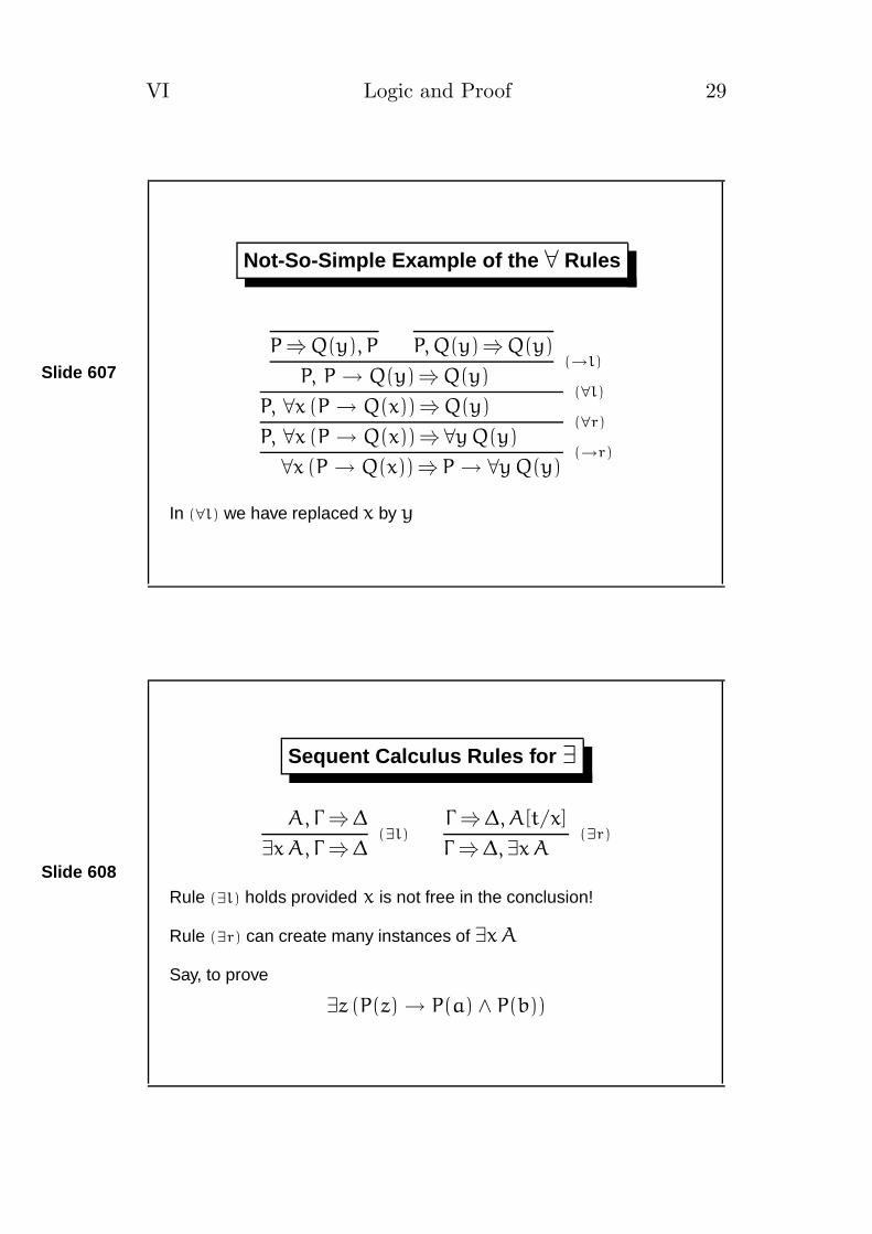
Not-So-Simple Example of the ∀ Rules
P⇒Q(y), P P, Q(y)⇒Q(y)
P, P → Q(y)⇒Q(y)(→l)
P, ∀x (P → Q(x))⇒Q(y)(∀l)
P, ∀x (P → Q(x))⇒ ∀y Q(y)(∀r)
∀x (P → Q(x))⇒ P → ∀y Q(y)(→r)
In (∀l) we have replaced x by y
Slide 608
Sequent Calculus Rules for ∃
A, Γ⇒∆
∃x A, Γ⇒∆(∃l)
Γ⇒∆, A[t/x]
Γ⇒∆, ∃x A(∃r)
Rule (∃l) holds provided x is not free in the conclusion!
Rule (∃r) can create many instances of ∃x A
Say, to prove
∃z (P(z) → P(a) ∧ P(b))

VI Logic and Proof 30
Slide 609
Part of the ∃ Distributive Law
P(x)⇒ P(x), Q(x)
P(x)⇒ P(x) ∨Q(x)(∨r)
P(x)⇒ ∃y (P(y) ∨Q(y))(∃r)
∃x P(x)⇒ ∃y (P(y) ∨Q(y))(∃l)
similar
∃x Q(x)⇒ ∃y . . .(∃l)
∃x P(x) ∨ ∃x Q(x)⇒ ∃y (P(y) ∨Q(y))(∨l)
Second subtree proves ∃x Q(x)⇒ ∃y (P(y) ∨Q(y)) similarly
In (∃r) we have replaced y by x
Slide 610
A Failed Proof
P(x), Q(y)⇒ P(x) ∧Q(x)
P(x), Q(y)⇒ ∃z (P(z) ∧Q(z))(∃r)
P(x), ∃x Q(x)⇒ ∃z (P(z) ∧Q(z))(∃l)
∃x P(x), ∃x Q(x)⇒ ∃z (P(z) ∧Q(z))(∃l)
∃x P(x) ∧ ∃x Q(x)⇒ ∃z (P(z) ∧Q(z))(∧l)
We cannot use (∃l) twice with the same variable
We rename the bound variable in ∃x Q(x) and get ∃y Q(y)

VII Logic and Proof 31
Slide 701
Clause Form
Clause: a disjunction of literals
¬K1 ∨ · · · ∨ ¬Km ∨ L1 ∨ · · · ∨ Ln
Set notation: {¬K1, . . . , ¬Km, L1, . . . , Ln}
Kowalski notation: K1, · · · , Km → L1, · · · , Ln
L1, · · · , Ln ← K1, · · · , Km
Empty clause: �
EMPTY CLAUSE MEANS CONTRADICTION!
Slide 702
Outline of Clause Form Methods
To prove A, obtain a contradiction from ¬A:
1. Translate ¬A into CNF as A1 ∧ · · · ∧Am
2. This is the set of clauses A1, . . ., Am
3. Transform the clause set, preserving consistency
Empty clause refutes ¬A
Empty clause set means ¬A is satisfiable

VII Logic and Proof 32
Slide 703
The Davis-Putnam-Logeman-Loveland Method
1. Delete tautological clauses: {P, ¬P, . . .}
2. For each unit clause {L},
• delete all clauses containing L
• delete ¬L from all clauses
3. Delete all clauses containing pure literals
4. Perform a case split on some literal
It’s a decision procedure: it finds either a contradiction or a model.
Slide 704
Davis-Putnam on a Non-Tautology
Consider P ∨Q → Q ∨ R
Clauses are {P, Q} {¬Q} {¬R}
{P, Q} {¬Q} {¬R} initial clauses
{P} {¬R} unit ¬Q
{¬R} unit P (also pure)
unit ¬R (also pure)
Clauses satisfiable by P 7→ t, Q 7→ f , R 7→ f
VII Logic and Proof 33
Slide 705
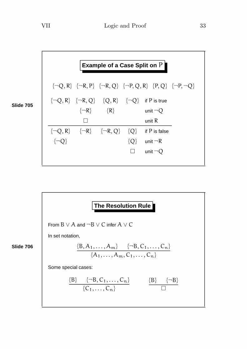
Example of a Case Split on P
{¬Q, R} {¬R, P} {¬R, Q} {¬P, Q, R} {P, Q} {¬P, ¬Q}
{¬Q, R} {¬R, Q} {Q, R} {¬Q} if P is true
{¬R} {R} unit ¬Q
� unit R
{¬Q, R} {¬R} {¬R, Q} {Q} if P is false
{¬Q} {Q} unit ¬R
� unit ¬Q
Slide 706
The Resolution Rule
From B ∨A and ¬B ∨ C infer A ∨ C
In set notation,
{B, A1, . . . , Am} {¬B, C1, . . . , Cn}
{A1, . . . , Am, C1, . . . , Cn}
Some special cases:
{B} {¬B, C1, . . . , Cn}
{C1, . . . , Cn}
{B} {¬B}
�

VII Logic and Proof 34
Slide 707
Simple Example: Proving P ∧Q → Q ∧ P
Hint: use ¬(A → B) ' A ∧ ¬B
1. Negate! ¬[P ∧Q → Q ∧ P]
2. Push ¬ in: (P ∧Q) ∧ ¬(Q ∧ P)
(P ∧Q) ∧ (¬Q ∨ ¬P)
Clauses: {P} {Q} {¬Q, ¬P}
Resolve {P} and {¬Q, ¬P} getting {¬Q}
Resolve {Q} and {¬Q} getting �
Slide 708
Another Example
Refute ¬[(P ∨Q) ∧ (P ∨ R) → P ∨ (Q ∧ R)]
From (P ∨Q) ∧ (P ∨ R), get clauses {P, Q} and {P, R}
From ¬ [P ∨ (Q ∧ R)] get clauses {¬P} and {¬Q, ¬R}
Resolve {¬P} and {P, Q} getting {Q}
Resolve {¬P} and {P, R} getting {R}
Resolve {Q} and {¬Q, ¬R} getting {¬R}
Resolve {R} and {¬R} getting �

VII Logic and Proof 35
Slide 709
The Saturation Algorithm
At start, all clauses are passive. None are active.
1. Transfer a clause (current) from passive to active.
2. Form all resolvents between current and an active clause.
3. Use new clauses to simplify both passive and active.
4. Put the new clauses into passive.
Repeat until CONTRADICTION found or passive becomes empty.
Slide 710
Refinements of Resolution
Preprocessing: removing tautologies, symmetries . . .
Set of Support : working from the goal
Weighting: priority to the smallest clauses
Subsumption: deleting redundant clauses
Hyper-resolution: avoiding intermediate clauses
Indexing: data structures for speed

VIII Logic and Proof 36
Slide 801
Reducing FOL to Propositional Logic
Prenex : Move quantifiers to the front
Skolemize: Remove quantifiers, preserving consistency
Herbrand models: Reduce the class of interpretations
Herbrand’s Thm: Contradictions have finite, ground proofs
Unification: Automatically find the right instantiations
Finally, combine unification with resolution
Slide 802
Prenex Normal Form
Convert to Negation Normal Form using additionally
¬(∀x A) ' ∃x ¬A
¬(∃x A) ' ∀x ¬A
Then move quantifiers to the front using
(∀x A) ∧ B ' ∀x (A ∧ B)
(∀x A) ∨ B ' ∀x (A ∨ B)
and the similar rules for ∃

VIII Logic and Proof 37
Slide 803
Skolemization
Take a formula of the form
∀x1 ∀x2 · · · ∀xk ∃y A
Choose a new k-place function symbol, say f
Delete ∃y and replace y by f(x1, x2, . . . , xk). We get
∀x1 ∀x2 · · · ∀xk A[f(x1, x2, . . . , xk)/y]
Repeat until no ∃ quantifiers remain
Slide 804
Example of Conversion to Clauses
For proving ∃x [P(x) → ∀y P(y)]
¬ [∃x [P(x) → ∀y P(y)]] negated goal
∀x [P(x) ∧ ∃y ¬P(y)] conversion to NNF
∀x ∃y [P(x) ∧ ¬P(y)] pulling ∃ out
∀x [P(x) ∧ ¬P(f(x))] Skolem term f(x)
{P(x)} {¬P(f(x))} Final clauses

VIII Logic and Proof 38
Slide 805
Correctness of Skolemization
The formula ∀x ∃y A is consistent
⇐⇒ it holds in some interpretation I = (D, I)
⇐⇒ for all x ∈ D there is some y ∈ D such that A holds
⇐⇒ some function f in D→ D yields suitable values of y
⇐⇒ A[f(x)/y] holds in some I ′ extending I so that f denotes f
⇐⇒ the formula ∀x A[f(x)/y] is consistent.
Slide 806
Herbrand Interpretations for a set of clauses S
H0def= the set of constants in S
Hi+1def= Hi ∪ {f(t1, . . . , tn) | t1, . . . , tn ∈ Hi
and f is an n-place function symbol in S}
Hdef=
⋃
i≥0
Hi Herbrand Universe
HBdef= {P(t1, . . . , tn) | t1, . . . , tn ∈ H
and P is an n-place predicate symbol in S}

VIII Logic and Proof 39
Slide 807
Example of an Herbrand Model
¬even(1)
even(2)
even(X · Y)← even(X), even(Y)
clauses
H = {1, 2, 1 · 1, 1 · 2, 2 · 1, 2 · 2, 1 · (1 · 1), . . .}
HB = {even(1), even(2), even(1 · 1), even(1 · 2), . . .}
I[even] = {even(2), even(1 · 2), even(2 · 1), even(2 · 2), . . .}
(for model where · means product; could instead use sum!)
Slide 808
A Key Fact about Herbrand Interpretations
Let S be a set of clauses.
S is unsatisfiable ⇐⇒ no Herbrand interpretation satisfies S
• Holds because some Herbrand model mimicks every ‘real’ model
• We must consider only a small class of models
• Herbrand models are syntactic, easily processed by computer

VIII Logic and Proof 40
Slide 809
Herbrand’s Theorem
Let S be a set of clauses.
S is unsatisfiable ⇐⇒ there is a finite unsatisfiable set S ′ of ground
instances of clauses of S.
• Finite: we can compute it
• Instance: result of substituting for variables
• Ground: and no variables remain: it’s propositional!

IX Logic and Proof 41
Slide 901
Unification
Finding a common instance of two terms
• Logic programming (Prolog)
• Polymorphic type-checking (ML)
• Constraint satisfaction problems
• Resolution theorem proving for FOL
• Many other theorem proving methods
Slide 902
Substitutions
A finite set of replacements
θ = [t1/x1, . . . , tk/xk]
where x1, . . ., xk are distinct variables and ti 6= xi
f(t, u)θ = f(tθ, uθ) (terms)
P(t, u)θ = P(tθ, uθ) (literals)
{L1, . . . , Lm}θ = {L1θ, . . . , Lmθ} (clauses)

IX Logic and Proof 42
Slide 903
Composing Substitutions
Composition of φ and θ, written φ ◦ θ, satisfies for all terms t
t(φ ◦ θ) = (tφ)θ
It is defined by (for all relevant x)
φ ◦ θdef= [ (xφ)θ / x, . . . ]
Consequences include θ ◦ [] = θ, and associativity :
(φ ◦ θ) ◦ σ = φ ◦ (θ ◦ σ)
Slide 904
Most General Unifiers
θ is a unifier of terms t and u if tθ = uθ
θ is more general than φ if φ = θ ◦ σ
θ is most general if it is more general than every other unifier
If θ unifies t and u then so does θ ◦ σ:
t(θ ◦ σ) = tθσ = uθσ = u(θ ◦ σ)
A most general unifier of f(a, x) and f(y, g(z)) is [a/y, g(z)/x]
The common instance is f(a, g(z))

IX Logic and Proof 43
Slide 905
Algorithm for Unifying Two Terms
Represent terms by binary trees
Each term is a Variable x, y . . ., Constant a, b . . ., or Pair (t, t ′)
Constants do not unify with different Constants
Constants do not unify with Pairs
Variable x and term t: unifier is [t/x] — unless x occurs in t
Cannot unify f(x) with x!
Slide 906
Unifying Two Pairs
θ ◦ θ ′ unifies (t, t ′) with (u, u ′)
if θ unifies t with u and θ ′ unifies t ′θ with u ′θ
(t, t ′)(θ ◦ θ ′) = (t, t ′)θθ ′
= (tθθ ′, t ′θθ ′)
= (uθθ ′, u ′θθ ′)
= (u, u ′)θθ ′
= (u, u ′)(θ ◦ θ ′)

IX Logic and Proof 44
Slide 907
Examples of Unification
f(x, b) f(x, x) f(x, x) j(x, x, z)
f(a, y) f(a, b) f(y, g(y)) j(w, a, h(w))
f(a, b) ? ? j(a, a, h(a))
[a/x, b/y] FAIL FAIL [a/w, a/x, h(a)/z]
We always get a most general unifier
Slide 908
Theorem-Proving Examples
(∃y ∀x R(x, y)) → (∀x ∃y R(x, y))
Clauses after negation are {R(x, a)} and {¬R(b, y)}
R(x, a) and R(b, y) have unifier [b/x, a/y]: contradiction!
(∀x ∃y R(x, y)) → (∃y ∀x R(x, y))
Clauses after negation are {R(x, f(x))} and {¬R(g(y), y)}
R(x, f(x)) and R(g(y), y) are not unifiable: occurs check
Formula is not a theorem!

IX Logic and Proof 45
Slide 909
Variations on Unification
Efficient unification algorithms: near-linear time
Indexing & Discrimination networks: fast retrieval of a unifiable term
Order-sorted unification: type-checking in Haskell
Associative/commutative operators: problems in group theory
Higher-order unification: support λ-calculus
Boolean unification: reasoning about sets

X Logic and Proof 46
Slide 1001
Binary Resolution
{B, A1, . . . , Am} {¬D, C1, . . . , Cn}
{A1, . . . , Am, C1, . . . , Cn}σprovided Bσ = Dσ
First rename variables apart in the clauses! — say, to resolve
{P(x)} and {¬P(g(x))}
Always use a most general unifier (MGU)
Soundness? Same argument as for the propositional version
Slide 1002
Factorisation
Collapsing similar literals in one clause:
{B1, . . . , Bk, A1, . . . , Am}
{B1, A1, . . . , Am}σprovided B1σ = · · · = Bkσ
Normally combined with resolution
Prove ∀x ∃y ¬(P(y, x) ↔ ¬P(y, y))
The clauses are {¬P(y, a), ¬P(y, y)} {P(y, y), P(y, a)}
Factoring yields {¬P(a, a)} {P(a, a)}
Resolution yields the empty clause!

X Logic and Proof 47
Slide 1003
A Non-Trivial Example
∃x [P → Q(x)] ∧ ∃x [Q(x) → P] → ∃x [P ↔ Q(x)]
Clauses are {P, ¬Q(b)} {P, Q(x)} {¬P, ¬Q(x)} {¬P, Q(a)}
Resolve {P, ¬Q(b)} with {P, Q(x)} getting {P}
Resolve {¬P, ¬Q(x)} with {¬P, Q(a)} getting {¬P}
Resolve {P} with {¬P} getting �
Implicit factoring: {P, P} 7→ {P} Many other proofs!
Slide 1004
Prolog Clauses and Their Execution
At most one positive literal per clause!
Definite clause {¬A1, . . . , ¬Am, B} or B← A1, . . . , Am.
Goal clause {¬A1, . . . , ¬Am} or ← A1, . . . , Am.
Linear resolution: a program clause with last goal clause
Left-to-right through program clauses
Left-to-right through goal clause’s literals
Depth-first search: backtracks, but still incomplete
Unification without occurs check : fast, but unsound!

X Logic and Proof 48
Slide 1005
A (Pure) Prolog Program
parent(elizabeth,charles).
parent(elizabeth,andrew).
parent(charles,william).
parent(charles,henry).
parent(andrew,beatrice).
parent(andrew,eugenia).
grand(X,Z) :- parent(X,Y), parent(Y,Z).
cousin(X,Y) :- grand(Z,X), grand(Z,Y).
Slide 1006
Prolog Execution
:- cousin(X,Y).
:- grand(Z1,X), grand(Z1,Y).
:- parent(Z1,Y2), parent(Y2,X), grand(Z1,Y).
* :- parent(charles,X), grand(elizabeth,Y).
X=william :- grand(elizabeth,Y).
:- parent(elizabeth,Y5), parent(Y5,Y).
* :- parent(andrew,Y).
Y=beatrice :- �.
* = backtracking choice point
16 solutions including cousin(william,william)
and cousin(william,henry)

X Logic and Proof 49
Slide 1007
The Method of Model Elimination
A Prolog-like method; complete for First-Order Logic
Contrapositives: treat clause {A1, . . . , Am} as m clauses
A1 ← ¬A2, . . . , ¬Am
A2 ← ¬A3, . . . , ¬Am, ¬A1
...
Extension rule: when proving goal P, may assume ¬P
A brute force method: efficient but no refinements such as
subsumption
Slide 1008
A Survey of Automatic Theorem Provers
Hyper-resolution: Otter, Gandalf, SPASS, Vampire, . . .
Model Elimination: Prolog Technology Theorem Prover, SETHEO
Parallel ME: PARTHENON, PARTHEO
Higher-Order Logic: TPS, LEO
Tableau (sequent) based: LeanTAP, 3TAP, . . .

X Logic and Proof 50
Slide 1009
Approaches to Equality Reasoning
Equality is reflexive, symmetric, transitive
Equality is substitutive over functions, predicates
• Use specialized prover: Knuth-Bendix, . . .
• Assert axioms directly
• Paramodulation rule
{B[t], A1, . . . , Am} {t = u, C1, . . . , Cn}
{B[u], A1, . . . , Am, C1, . . . , Cn}

XI Logic and Proof 51
Slide 1101
Modal Operators
W: set of possible worlds (machine states, future times, . . .)
R: accessibility relation between worlds
(W, R) is called a modal frame
2A means A is necessarily true
3A means A is possibly true
}— in all accessible worlds
¬3A ' 2¬A A cannot be true ⇐⇒ A must be false
Slide 1102
Semantics of Propositional Modal Logic
For a particular frame (W, R)
An interpretation I maps the propositional letters to subsets of W
w A means A is true in world w
w P ⇐⇒ w ∈ I(P)
w A ∧ B⇐⇒ w A and w B
w 2A ⇐⇒ v A for all v such that R(w, v)
w 3A ⇐⇒ v A for some v such that R(w, v)

XI Logic and Proof 52
Slide 1103
Truth and Validity in Modal Logic
For a particular frame (W, R), and interpretation I
w A means A is true in world w
|=W,R,I A means w A for all w in W
|=W,R A means w A for all w and all I
|= A means |=W,R A for all frames; A is universally valid
. . . but typically we constrain R to be, say, transitive
All tautologies are universally valid
Slide 1104
A Hilbert-Style Proof System for K
Extend your favourite propositional proof system with
Dist 2(A → B) → (2A → 2B)
Inference Rule: Necessitation
A2A
Treat 3 as a definition
3Adef= ¬2¬A
XI Logic and Proof 53
Slide 1105
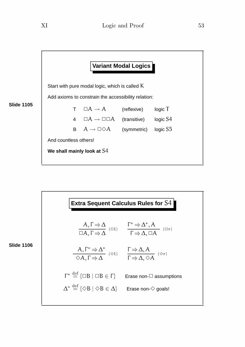
Variant Modal Logics
Start with pure modal logic, which is called K
Add axioms to constrain the accessibility relation:
T 2A → A (reflexive) logic T
4 2A → 22A (transitive) logic S4
B A → 23A (symmetric) logic S5
And countless others!
We shall mainly look at S4
Slide 1106
Extra Sequent Calculus Rules for S4
A, Γ⇒∆
2A, Γ⇒∆(2l)
Γ∗⇒∆∗, A
Γ⇒∆, 2A(2r)
A, Γ∗⇒∆∗
3A, Γ⇒∆(3l)
Γ⇒∆, A
Γ⇒∆, 3A(3r)
Γ∗def= {2B | 2B ∈ Γ } Erase non-2 assumptions
∆∗ def= {3B | 3B ∈ ∆} Erase non-3 goals!

XI Logic and Proof 54
Slide 1107
A Proof of the Distribution Axiom
A⇒B, A B, A⇒B
A → B, A⇒B(→l)
A → B, 2A⇒B(2l)
2(A → B), 2A⇒B(2l)
2(A → B), 2A⇒2B(2r)
And thus 2(A → B) → (2A → 2B)
Must apply (2r) first!
Slide 1108
Part of an Operator String Equivalence
3A⇒3A
23A⇒3A(2l)
323A⇒3A(3l)
2323A⇒3A(2l)
2323A⇒23A(2r)
In fact, 2323A ' 23A also 22A ' 2A
The S4 operator strings are 2 3 23 32 232 323

XI Logic and Proof 55
Slide 1109
Two Failed Proofs
⇒A
⇒3A(3r)
A⇒23A(2r)
B⇒A ∧ B
B⇒3(A ∧ B)(3r)
3A, 3B⇒3(A ∧ B)(3l)
Can extract a countermodel from the proof attempt

XII Logic and Proof 56
Slide 1201
Simplifying the Sequent Calculus
7 connectives (or 9 for modal logic):
¬ ∧ ∨ → ↔ ∀ ∃ (2 3)
Left and right: so 14 rules (or 18) plus basic sequent, cut
Idea! Work in Negation Normal Form
Fewer connectives: ∧ ∨ ∀ ∃ (2 3)
Sequents need one side only!
Slide 1202
Simplified Calculus: Left-Only
¬A, A, Γ⇒(basic) ¬A, Γ⇒ A, Γ⇒
Γ⇒(cut)
A, B, Γ⇒A ∧ B, Γ⇒
(∧l)A, Γ⇒ B, Γ⇒
A ∨ B, Γ⇒(∨l)
A[t/x], Γ⇒∀x A, Γ⇒
(∀l)A, Γ⇒
∃x A, Γ⇒(∃l)
Rule (∃l) holds provided x is not free in the conclusion!

XII Logic and Proof 57
Slide 1203
Left-Only Sequent Rules for S4
A, Γ⇒2A, Γ⇒
(2l)A, Γ∗⇒
3A, Γ⇒(3l)
Γ∗def= {2B | 2B ∈ Γ } Erase non-2 assumptions
From 14 (or 18) rules to 4 (or 6)
Left-side only system uses proof by contradiction
Right-side only system is an exact dual
Slide 1204
Proving ∀x (P → Q(x))⇒P → ∀y Q(y)
Move the right-side formula to the left and convert to NNF:
P ∧ ∃y ¬Q(y), ∀x (¬P ∨Q(x))⇒
P, ¬Q(y), ¬P⇒ P, ¬Q(y), Q(y)⇒P, ¬Q(y), ¬P ∨Q(y)⇒
(∨l)
P, ¬Q(y), ∀x (¬P ∨Q(x))⇒(∀l)
P, ∃y ¬Q(y), ∀x (¬P ∨Q(x))⇒(∃l)
P ∧ ∃y ¬Q(y), ∀x (¬P ∨Q(x))⇒(∧l)

XII Logic and Proof 58
Slide 1205
Adding Unification
Rule (∀l) now inserts a new free variable:
A[z/x], Γ⇒∀x A, Γ⇒
(∀l)
Let unification instantiate any free variable
In ¬A, B, Γ⇒ try unifying A with B to make a basic sequent
Updating a variable affects entire proof tree
What about rule (∃l)? Skolemize!
Slide 1206
Skolemization from NNF
Follow tree structure; don’t pull out quantifiers!
[∀y ∃z Q(y, z)] ∧ ∃x P(x) to [∀y Q(y, f(y))] ∧ P(a)
Better to push quantifiers in (called miniscoping)
Proving ∃x ∀y [P(x) → P(y)]
Negate; convert to NNF : ∀x ∃y [P(x) ∧ ¬P(y)]
Push in the ∃y : ∀x [P(x) ∧ ∃y ¬P(y)]
Push in the ∀x : ∀x P(x) ∧ ∃y ¬P(y)
Skolemize: ∀x P(x) ∧ ¬P(a)
XII Logic and Proof 59
Slide 1207
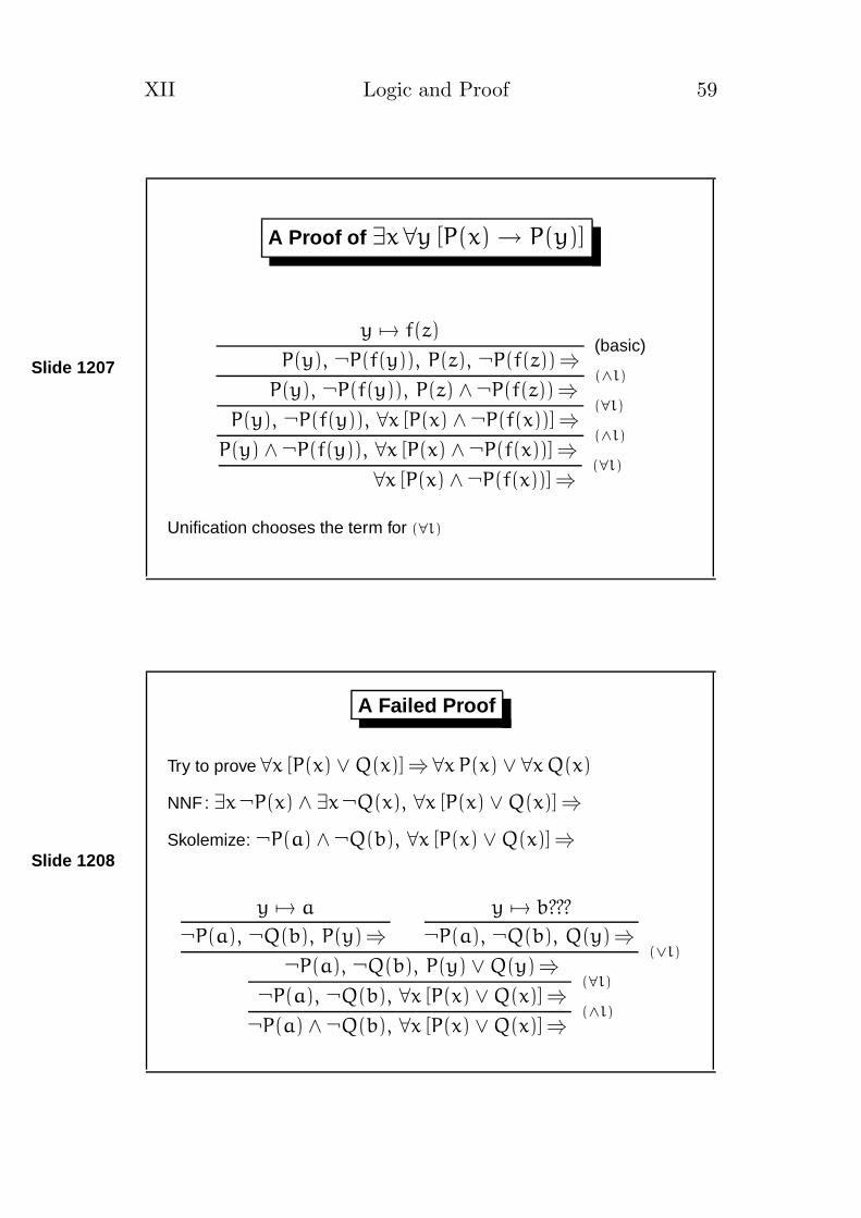
A Proof of ∃x ∀y [P(x) → P(y)]
y 7→ f(z)
P(y), ¬P(f(y)), P(z), ¬P(f(z))⇒(basic)
P(y), ¬P(f(y)), P(z) ∧ ¬P(f(z))⇒(∧l)
P(y), ¬P(f(y)), ∀x [P(x) ∧ ¬P(f(x))]⇒(∀l)
P(y) ∧ ¬P(f(y)), ∀x [P(x) ∧ ¬P(f(x))]⇒(∧l)
∀x [P(x) ∧ ¬P(f(x))]⇒(∀l)
Unification chooses the term for (∀l)
Slide 1208
A Failed Proof
Try to prove ∀x [P(x) ∨Q(x)]⇒ ∀x P(x) ∨ ∀x Q(x)
NNF : ∃x ¬P(x) ∧ ∃x ¬Q(x), ∀x [P(x) ∨Q(x)]⇒
Skolemize: ¬P(a) ∧ ¬Q(b), ∀x [P(x) ∨Q(x)]⇒
y 7→ a
¬P(a), ¬Q(b), P(y)⇒y 7→ b???
¬P(a), ¬Q(b), Q(y)⇒¬P(a), ¬Q(b), P(y) ∨Q(y)⇒
(∨l)
¬P(a), ¬Q(b), ∀x [P(x) ∨Q(x)]⇒(∀l)
¬P(a) ∧ ¬Q(b), ∀x [P(x) ∨Q(x)]⇒(∧l)

XII Logic and Proof 60
Slide 1209
The World’s Smallest Theorem Prover?
prove((A,B),UnExp,Lits,FreeV,VarLim) :- !,
prove(A,[B|UnExp],Lits,FreeV,VarLim).
prove((A;B),UnExp,Lits,FreeV,VarLim) :- !,
prove(A,UnExp,Lits,FreeV,VarLim),
prove(B,UnExp,Lits,FreeV,VarLim).
prove(all(X,Fml),UnExp,Lits,FreeV,VarLim) :- !,
\+ length(FreeV,VarLim),
copy_term((X,Fml,FreeV),(X1,Fml1,FreeV)),
append(UnExp,[all(X,Fml)],UnExp1),
prove(Fml1,UnExp1,Lits,[X1|FreeV],VarLim).
prove(Lit,_,[L|Lits],_,_) :-
(Lit = -Neg; -Lit = Neg) ->
(unify(Neg,L); prove(Lit,[],Lits,_,_)).
prove(Lit,[Next|UnExp],Lits,FreeV,VarLim) :-
prove(Next,UnExp,[Lit|Lits],FreeV,VarLim).