log-linear models in nlp noah a. smith department of computer science / center for language and...
Post on 19-Dec-2015
214 views
TRANSCRIPT
Log-Linear Models in NLP
Noah A. SmithDepartment of Computer Science /
Center for Language and Speech ProcessingJohns Hopkins [email protected]
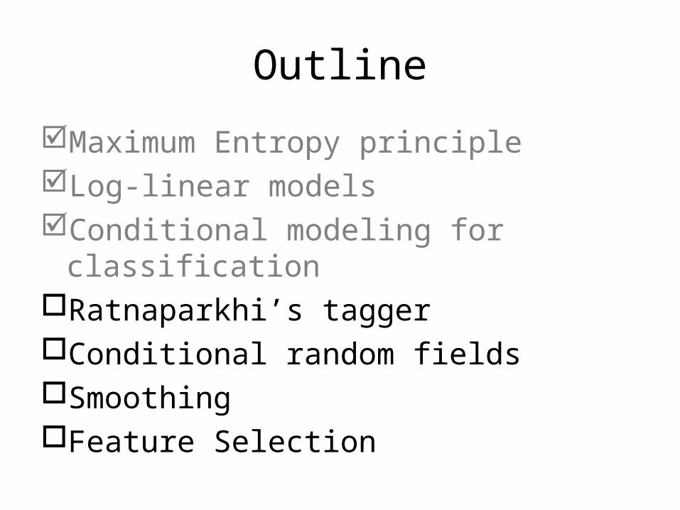
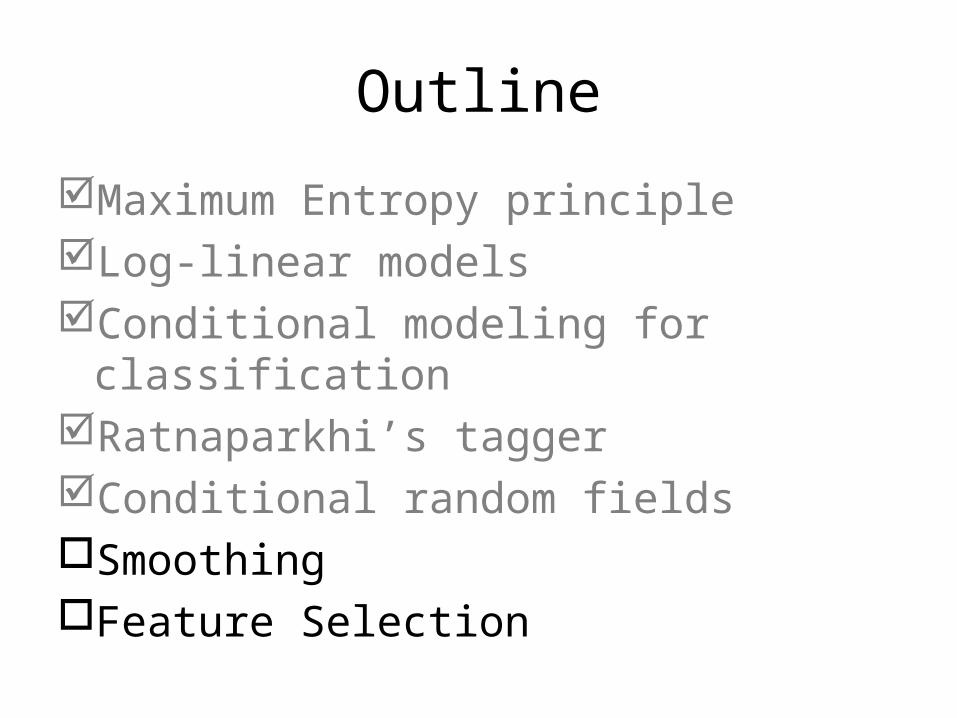
Outline
Maximum Entropy principleLog-linear modelsConditional modeling for
classificationRatnaparkhi’s tagger Conditional random fieldsSmoothingFeature Selection
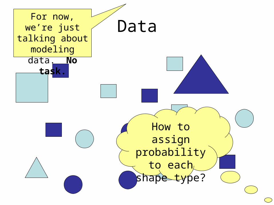
DataFor now, we’re
just talking about modeling data. No task.
How to assign
probability to each
shape type?
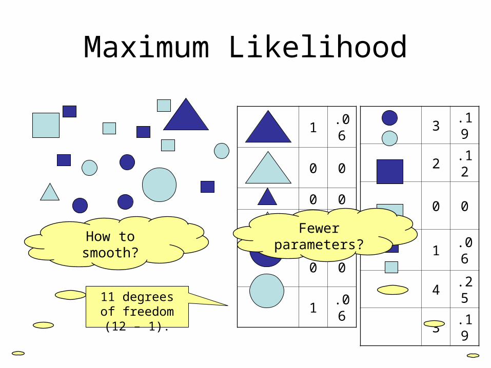
3.19
2.12
0 0
1.06
4.25
3.19
Maximum Likelihood
1.06
0 0
0 0
1.06
0 0
1.06
11 degrees of freedom (12 –
1).
How to smooth?
Fewer parameters?
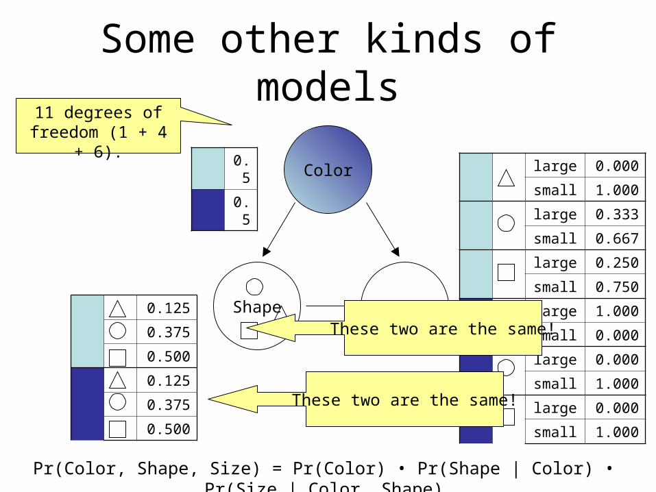
Some other kinds of models
Color
Shape Size
Pr(Color, Shape, Size) = Pr(Color) • Pr(Shape | Color) • Pr(Size | Color, Shape)
0.5
0.5
0.125
0.375
0.500
0.125
0.375
0.500
large 0.000
small 1.000
large 0.333
small 0.667
large 0.250
small 0.750
large 1.000
small 0.000
large 0.000
small 1.000
large 0.000
small 1.000
11 degrees of freedom (1 + 4 +
6).
These two are the same!
These two are the same!
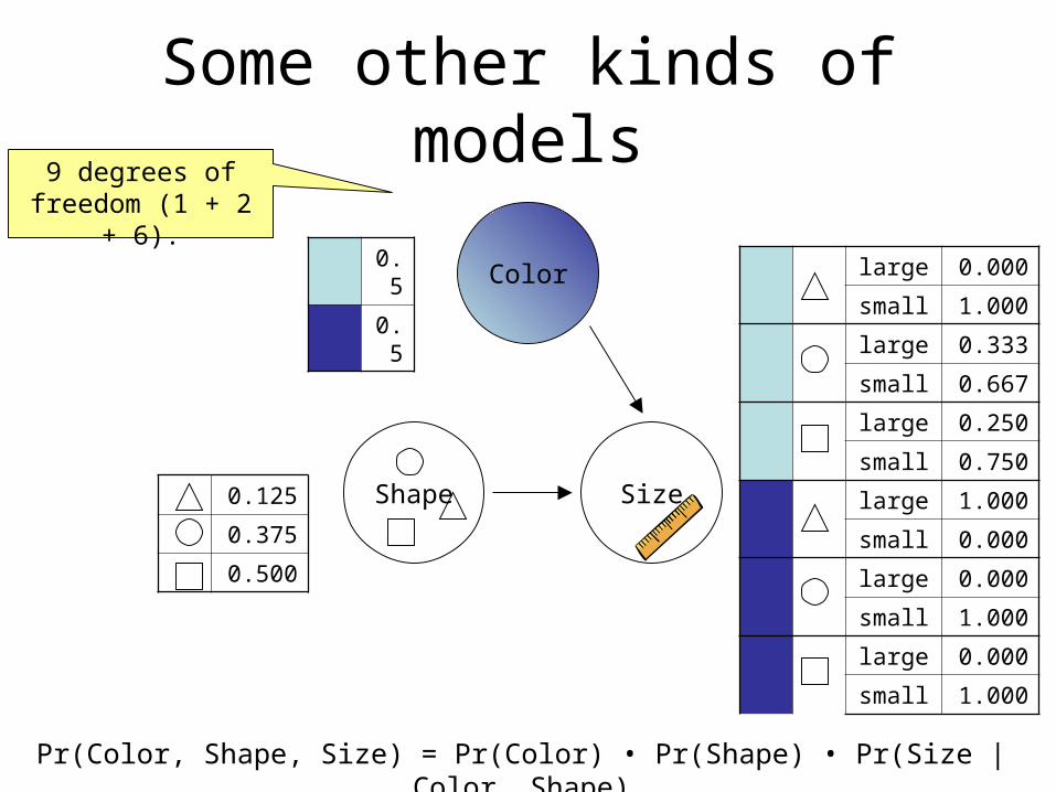
Some other kinds of models
Color
Shape Size
Pr(Color, Shape, Size) = Pr(Color) • Pr(Shape) • Pr(Size | Color, Shape)
0.5
0.5
0.125
0.375
0.500
9 degrees of freedom (1 + 2 +
6).large 0.000
small 1.000
large 0.333
small 0.667
large 0.250
small 0.750
large 1.000
small 0.000
large 0.000
small 1.000
large 0.000
small 1.000
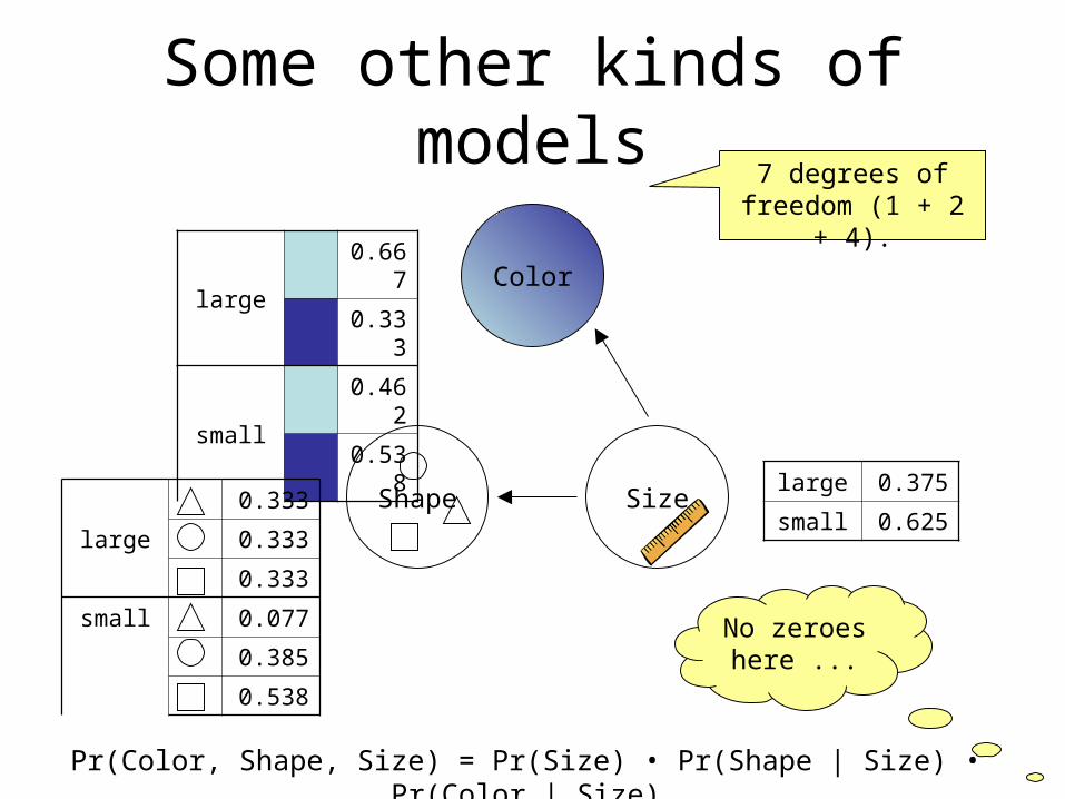
Some other kinds of models
Color
Shape Size
Pr(Color, Shape, Size) = Pr(Size) • Pr(Shape | Size) • Pr(Color | Size)
large
0.667
0.333
small
0.462
0.538
large
0.333
0.333
0.333
small 0.077
0.385
0.538
large 0.375
small 0.625
7 degrees of freedom (1 + 2 +
4).
No zeroes here ...
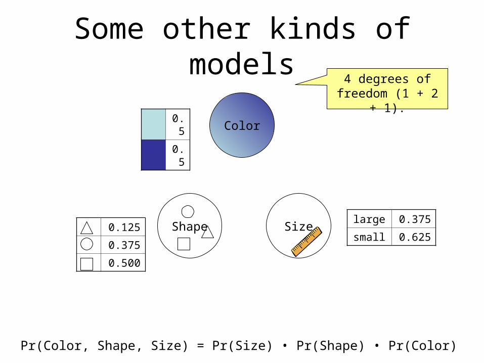
Some other kinds of models
Color
Shape Size
Pr(Color, Shape, Size) = Pr(Size) • Pr(Shape) • Pr(Color)
0.125
0.375
0.500
large 0.375
small 0.625
4 degrees of freedom (1 + 2 +
1).0.5
0.5
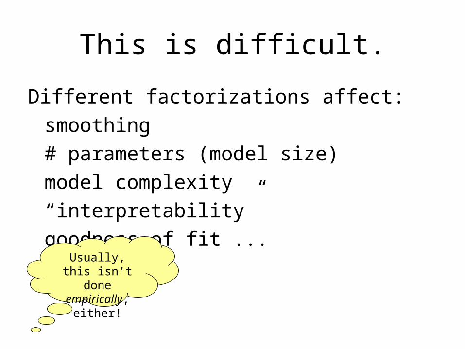
This is difficult.
Different factorizations affect:smoothing
# parameters (model size)model complexity
“interpretability”goodness of fit
...Usually, this
isn’t done empirically,
either!
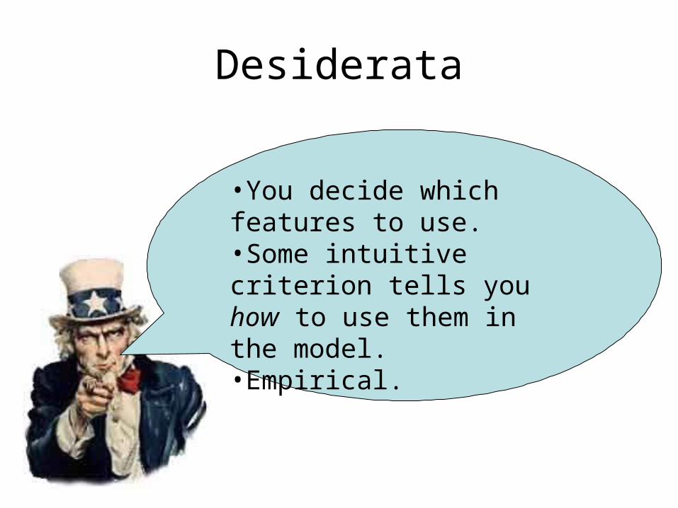
Desiderata
•You decide which features to use.•Some intuitive criterion tells you how to use them in the model.•Empirical.
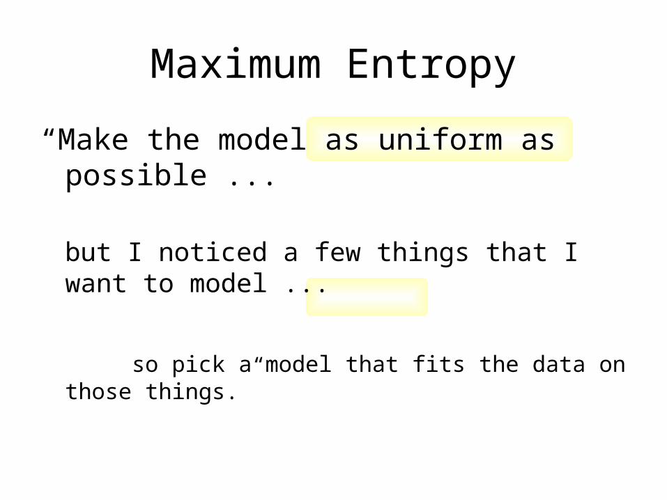
Maximum Entropy
“Make the model as uniform as possible ...
but I noticed a few things that I want to model ...
so pick a model that fits the data on those things.”
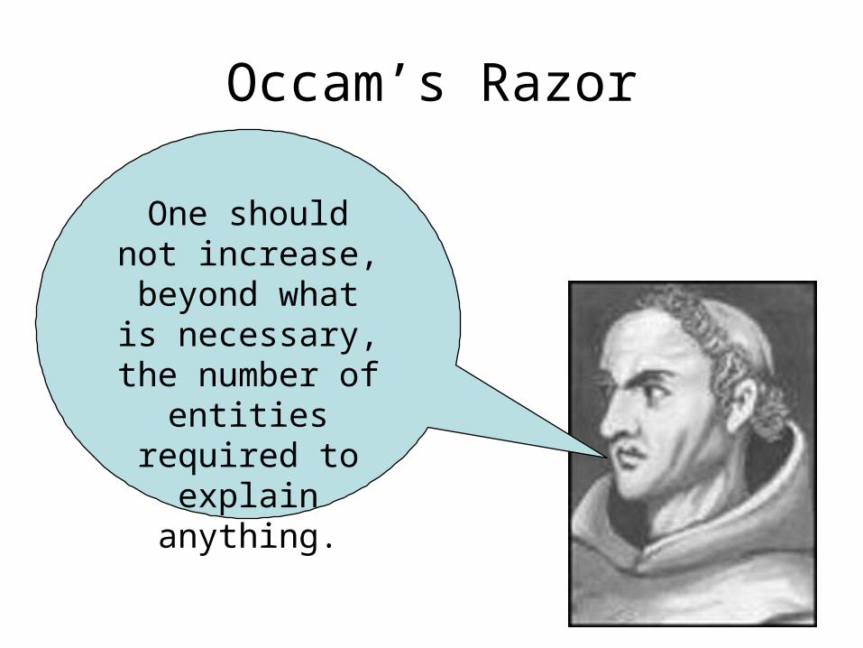
Occam’s Razor
One should not increase,
beyond what is necessary, the
number of entities
required to explain
anything.
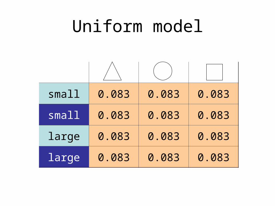
Uniform model
small 0.083 0.083 0.083
small 0.083 0.083 0.083
large 0.083 0.083 0.083
large 0.083 0.083 0.083
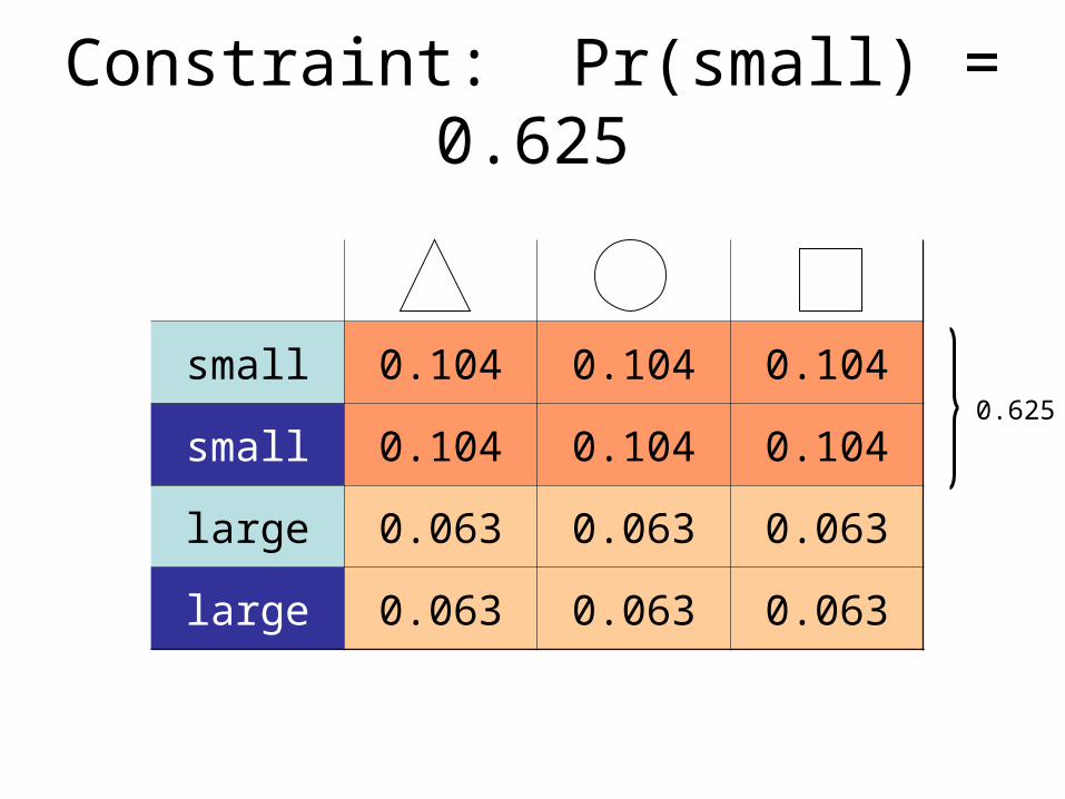
Constraint: Pr(small) = 0.625
small 0.104 0.104 0.104
small 0.104 0.104 0.104
large 0.063 0.063 0.063
large 0.063 0.063 0.063
0.625
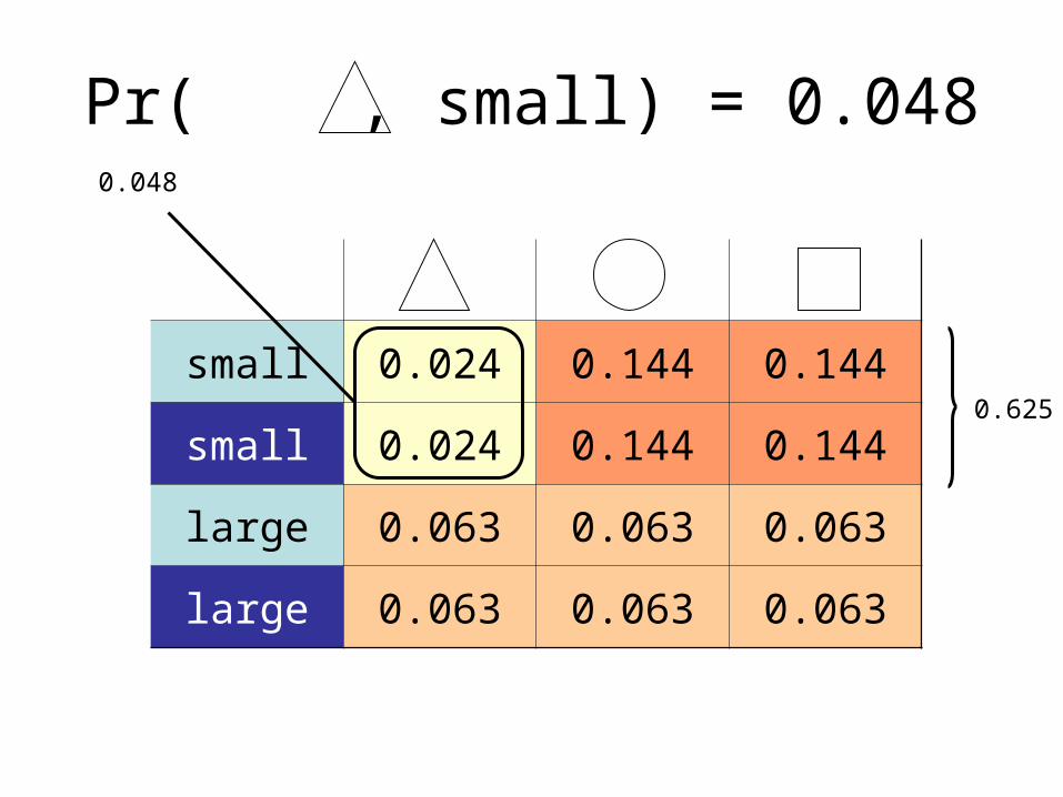
Pr( , small) = 0.048
small 0.024 0.144 0.144
small 0.024 0.144 0.144
large 0.063 0.063 0.063
large 0.063 0.063 0.063
0.625
0.048
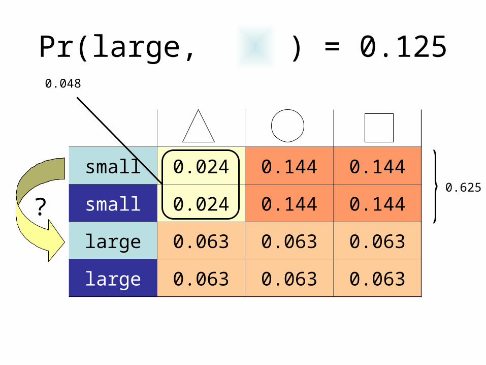
Pr(large, ) = 0.125
small 0.024 0.144 0.144
small 0.024 0.144 0.144
large 0.063 0.063 0.063
large 0.063 0.063 0.063
0.625
?
0.048
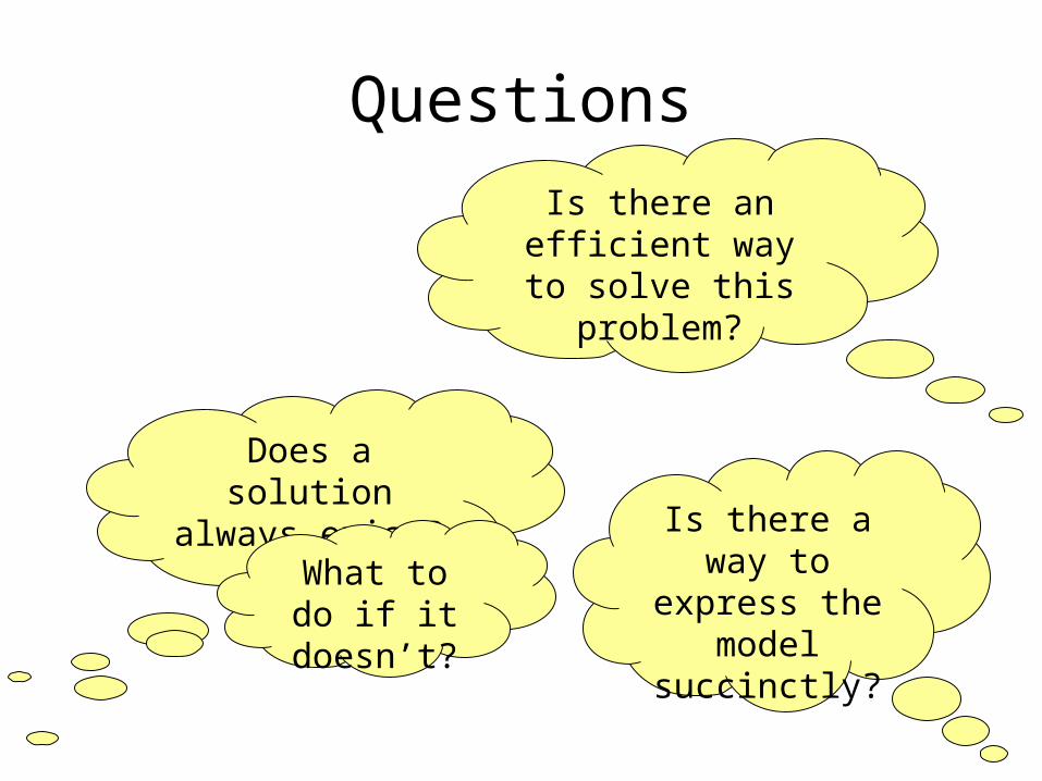
Questions
Does a solution always exist?
Is there a way to express the
model succinctly?
Is there an efficient way to
solve this problem?
What to do if it
doesn’t?
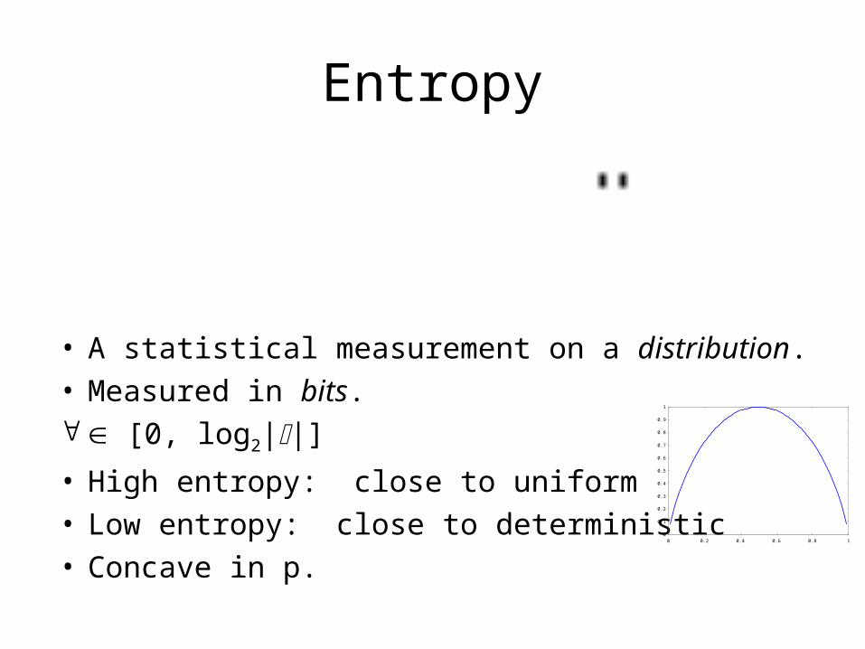
Entropy
• A statistical measurement on a distribution.• Measured in bits. [0, log2||]• High entropy: close to uniform• Low entropy: close to deterministic• Concave in p.
0
0.1
0.2
0.3
0.4
0.5
0.6
0.7
0.8
0.9
1
0 0.2 0.4 0.6 0.8 1
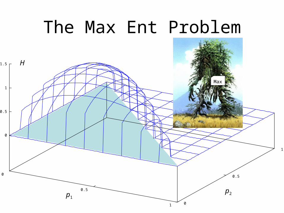
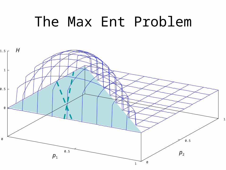
The Max Ent Problem
0
0.5
1 0
0.5
1
0
0.5
1
1.5
p1p2
H
Max
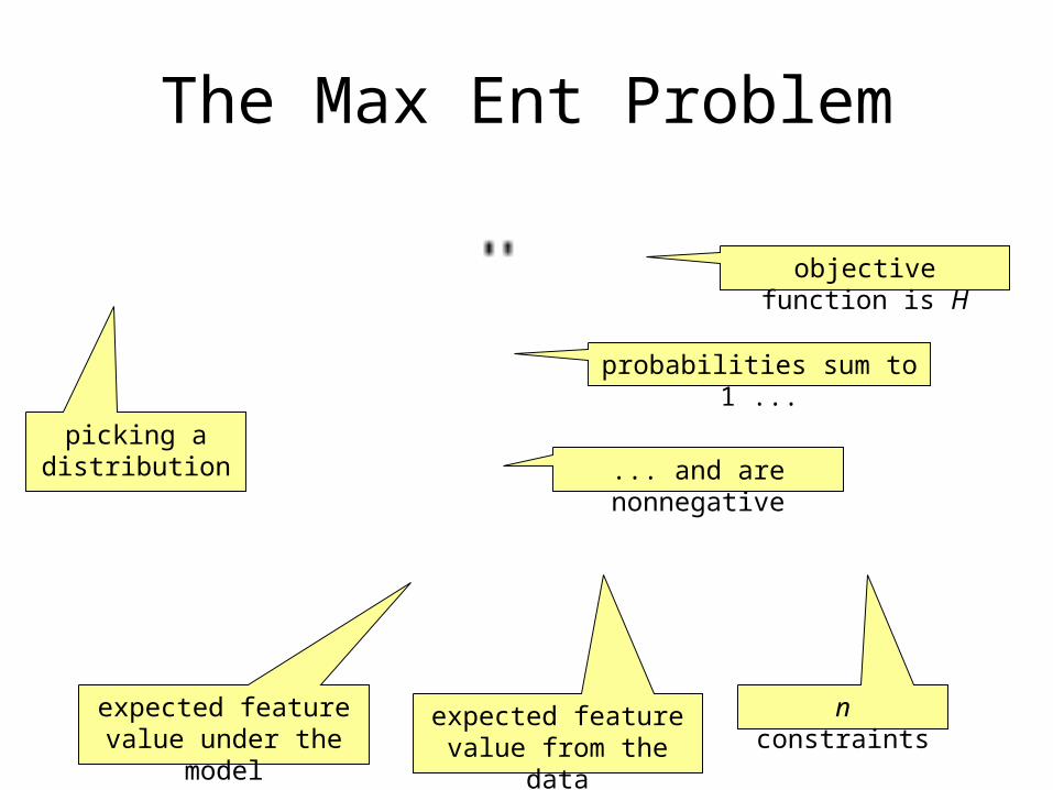
The Max Ent Problem
objective function is H
probabilities sum to 1 ...
... and are nonnegative
expected feature value under the
model
expected feature value from the data
n constraints
picking a distribution
The Max Ent Problem
0
0.5
1 0
0.5
1
0
0.5
1
1.5
p1p2
H
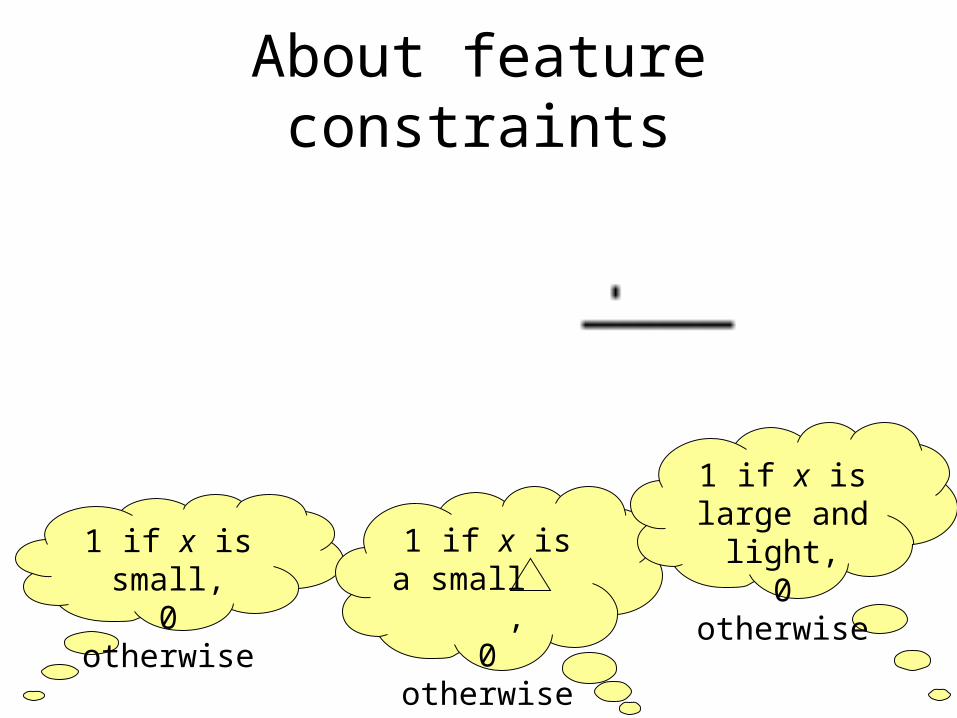
About feature constraints
1 if x is small,
0 otherwise
1 if x is a small ,
0 otherwise
1 if x is large and
light,0 otherwise
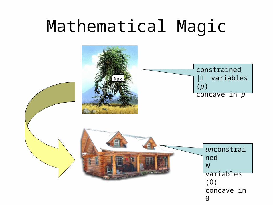
Mathematical Magic
Max
constrained|| variables (p)concave in p
unconstrainedN variables (θ)concave in θ
What’s the catch?
The model takes on a specific, parameterized form.
It can be shown that any max-ent model must take this form.
Outline
Maximum Entropy principleLog-linear modelsConditional modeling for
classificationRatnaparkhi’s tagger Conditional random fieldsSmoothingFeature Selection
Log-linear models
Log linear
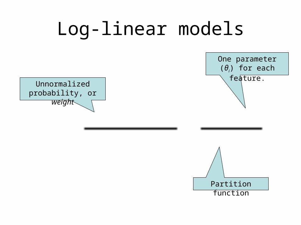
Log-linear models
Unnormalized probability, or
weight
Partition function
One parameter (θi) for each feature.
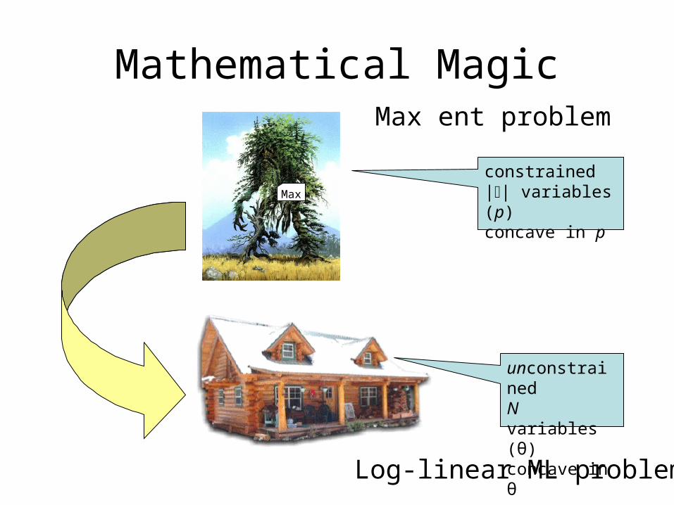
Mathematical Magic
Max
constrained|| variables (p)concave in p
unconstrainedN variables (θ)concave in θ
Max ent problem
Log-linear ML problem
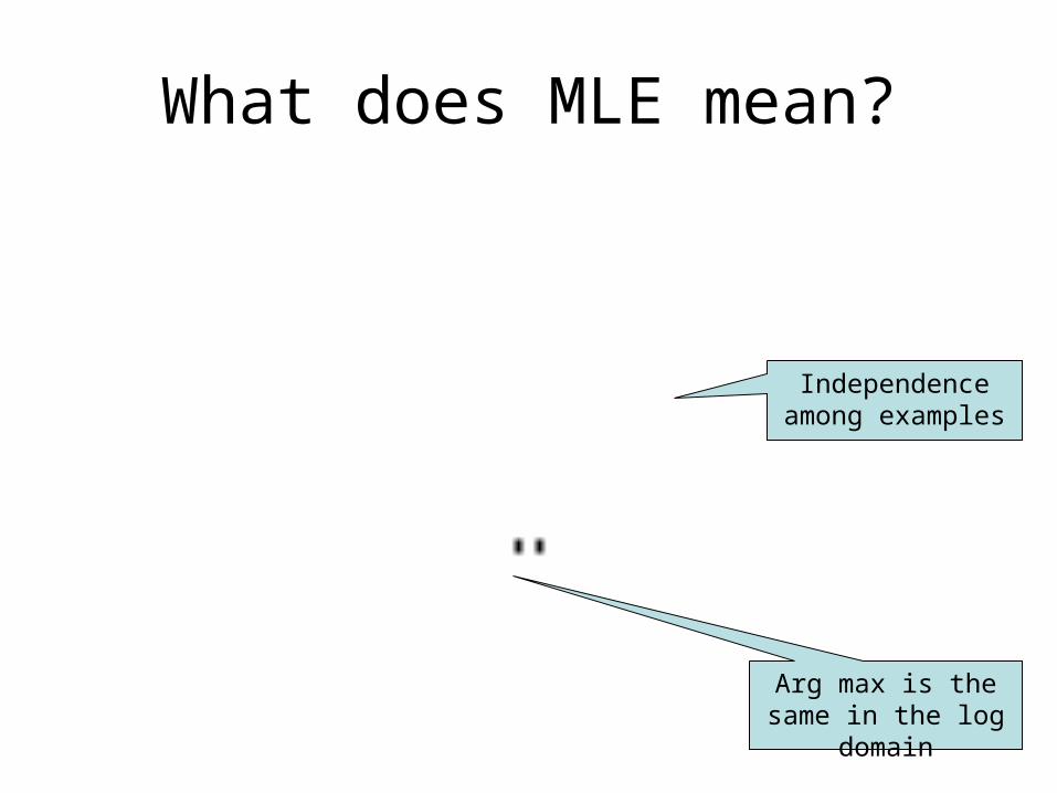
What does MLE mean?
Independence among examples
Arg max is the same in the log
domain
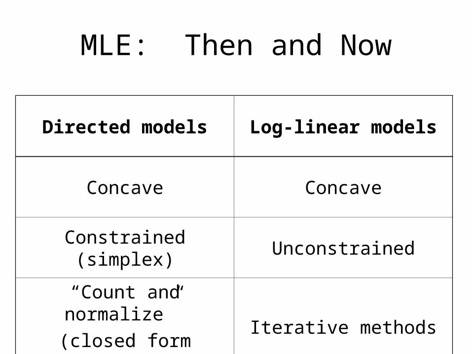
MLE: Then and Now
Directed models Log-linear models
Concave Concave
Constrained (simplex) Unconstrained
“Count and normalize”
(closed form solution)Iterative methods
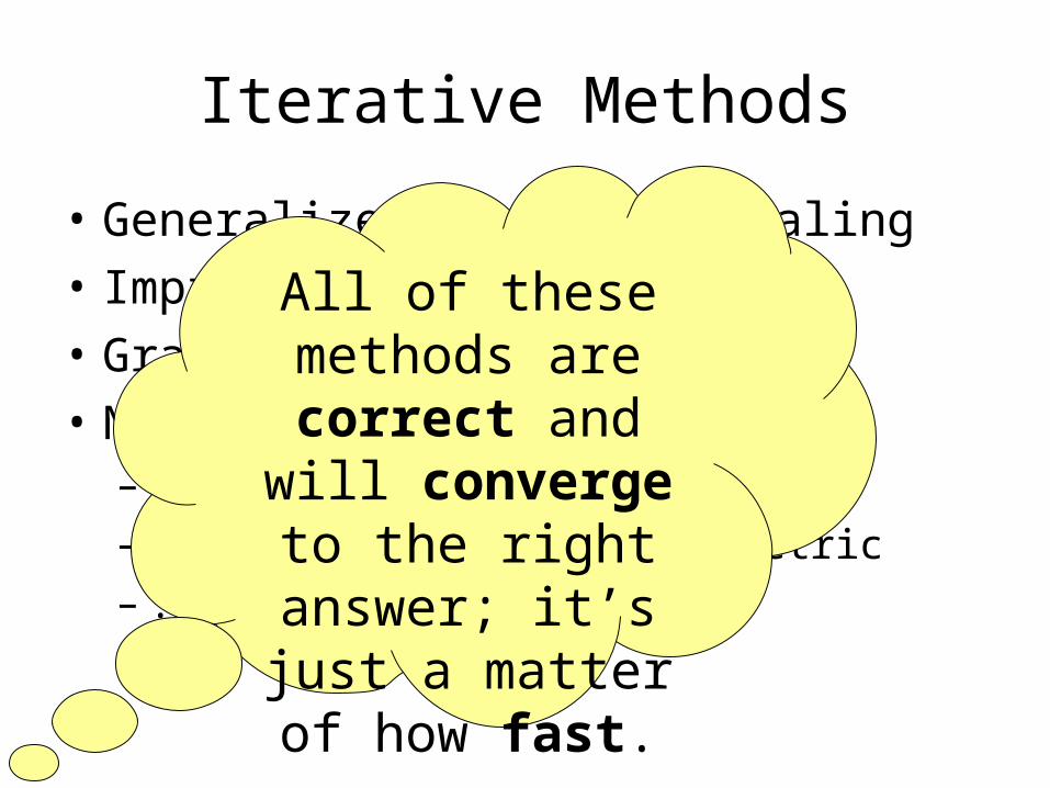
Iterative Methods
• Generalized Iterative Scaling• Improved Iterative Scaling• Gradient Ascent• Newton/Quasi-Newton Methods
– Conjugate Gradient– Limited-Memory Variable Metric– ...
All of these methods are
correct and will converge to the right answer; it’s just a matter of
how fast.
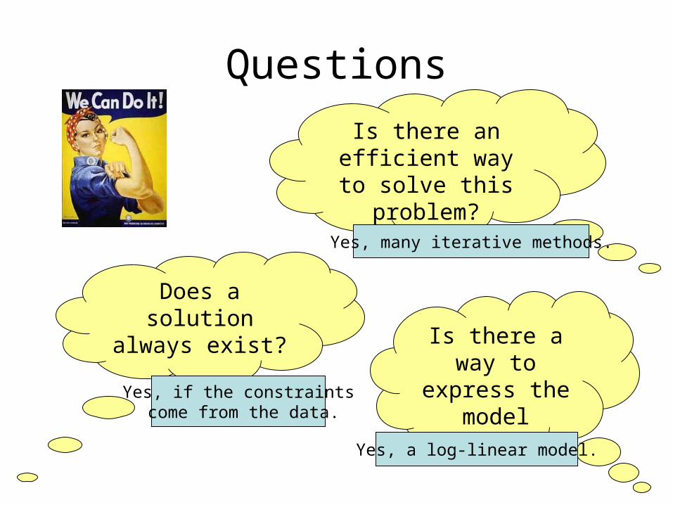
Questions
Does a solution always exist?
Is there a way to express the
model succinctly?
Is there an efficient way to
solve this problem?
Yes, if the constraints come from the data.
Yes, many iterative methods.
Yes, a log-linear model.
Outline
Maximum Entropy principleLog-linear modelsConditional modeling for
classificationRatnaparkhi’s tagger Conditional random fieldsSmoothingFeature Selection
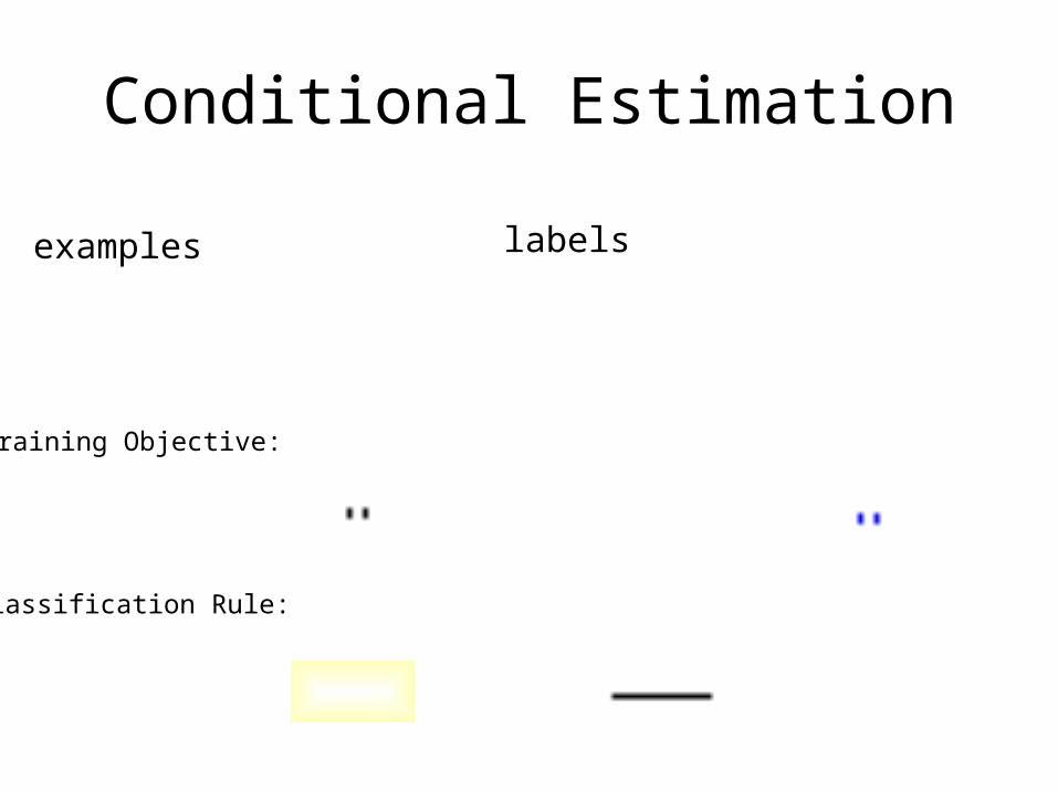
Conditional Estimation
Classification Rule:
Training Objective:
examples labels
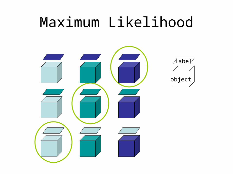
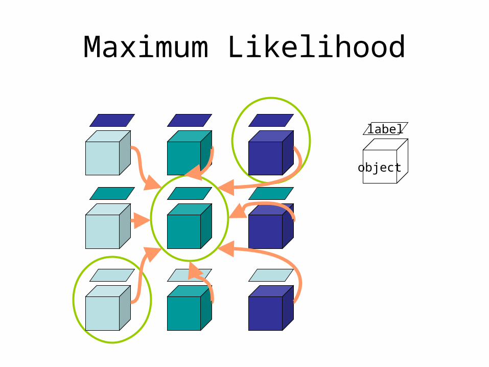
Maximum Likelihood
object
label
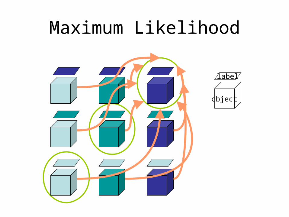
Maximum Likelihood
object
label
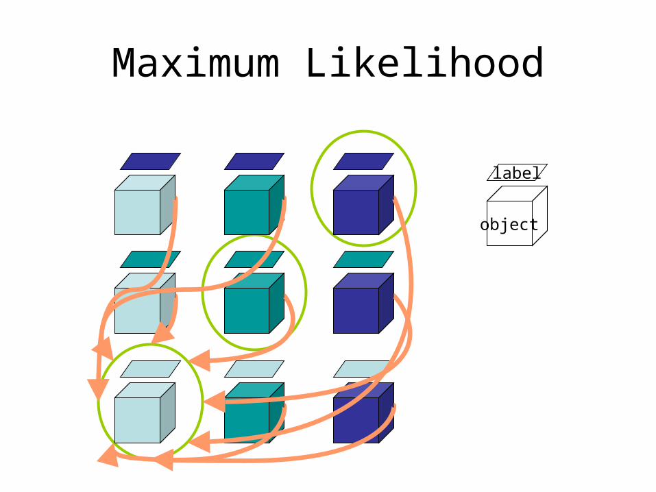
Maximum Likelihood
object
label
Maximum Likelihood
object
label
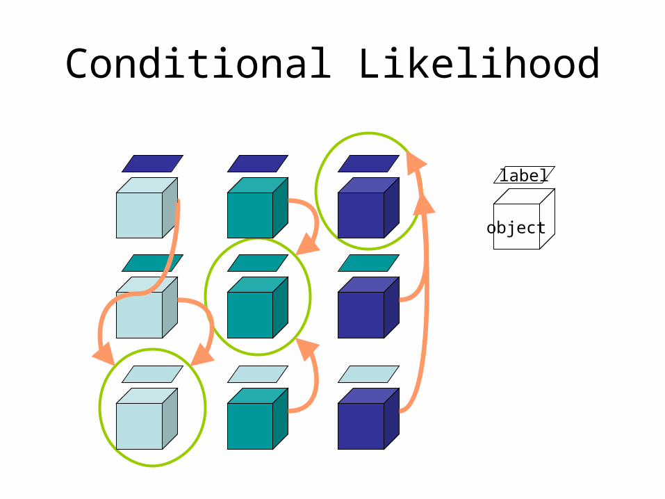
Conditional Likelihood
object
label
Remember:
log-linear models
conditional estimation
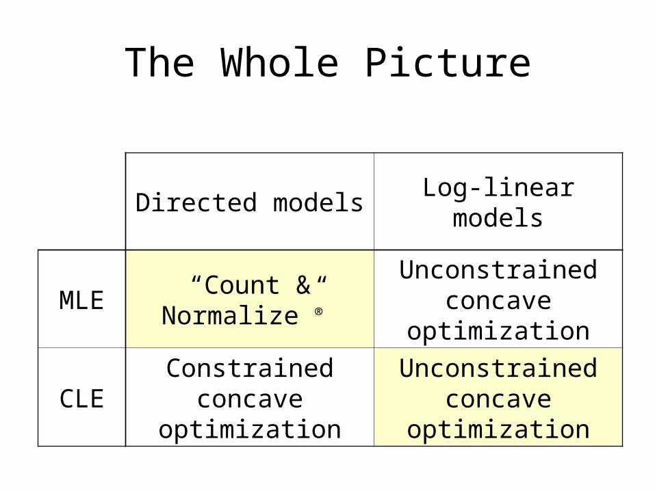
The Whole Picture
Directed models Log-linear models
MLE“Count &
Normalize”®
Unconstrained concave
optimization
CLEConstrained
concave optimization
Unconstrained concave
optimization
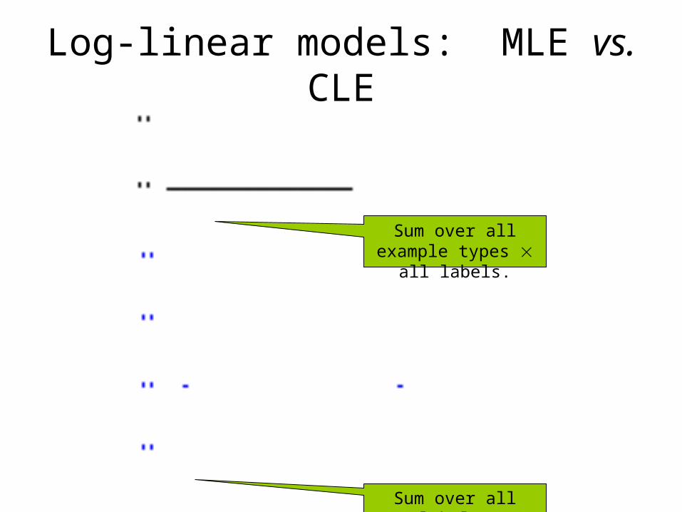
Log-linear models: MLE vs. CLE
Sum over all example types
all labels.
Sum over all labels.
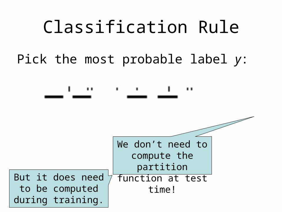
Classification Rule
Pick the most probable label y:
We don’t need to compute the
partition function at test time!But it does need to
be computed during training.
Outline
Maximum Entropy principleLog-linear modelsConditional modeling for
classificationRatnaparkhi’s tagger Conditional random fieldsSmoothingFeature Selection
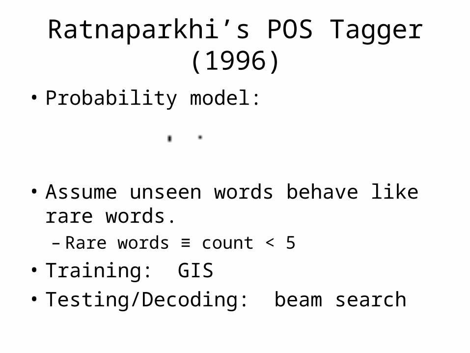
Ratnaparkhi’s POS Tagger (1996)
• Probability model:
• Assume unseen words behave like rare words.– Rare words ≡ count < 5
• Training: GIS• Testing/Decoding: beam search
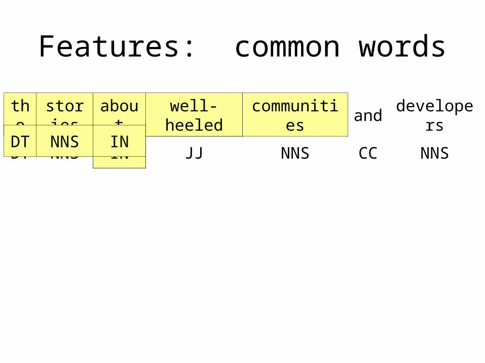
Features: common words
the
stories
about
well-heeled
communities
anddeveloper
s
DT
NNS IN JJ NNS CC NNS
about
IN
stories
IN
the
IN
well-heeled
IN
communities
INNNS INDT
NNS IN
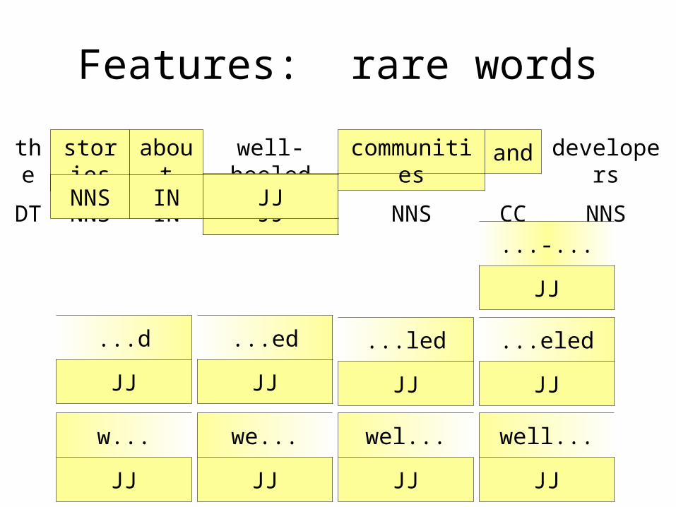
Features: rare words
the
stories
about
well-heeled
communities
anddeveloper
s
DT
NNS IN JJ NNS CC NNS
about
JJ
stories
JJ
communities
JJ
and
JJIN JJNNS IN JJ
w...
JJ
we...
JJ
wel...
JJ
well...
JJ
...d
JJ
...ed
JJ
...led
JJ
...eled
JJ
...-...
JJ
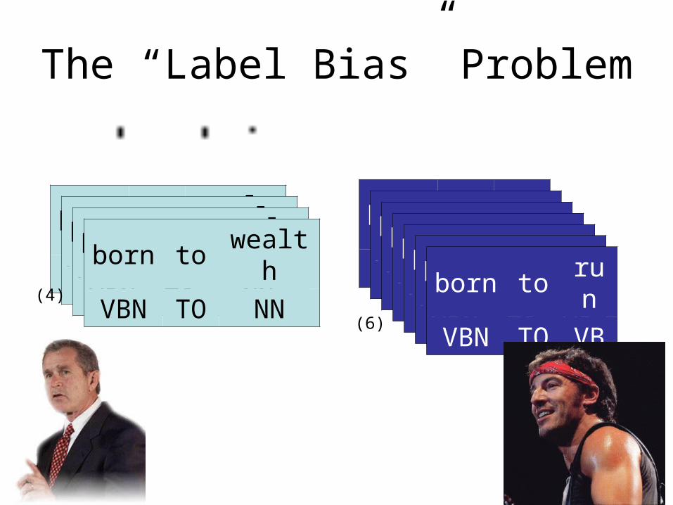
The “Label Bias” Problem
born towealt
h
VBN TO NN
born torun
VBN TO VBborn to
wealth
VBN TO NN
born towealt
h
VBN TO NN
born towealt
h
VBN TO NN
born torun
VBN TO VB
born torun
VBN TO VB
born torun
VBN TO VB
born torun
VBN TO VB
born torun
VBN TO VB
born torun
VBN TO VB
(4)
(6)
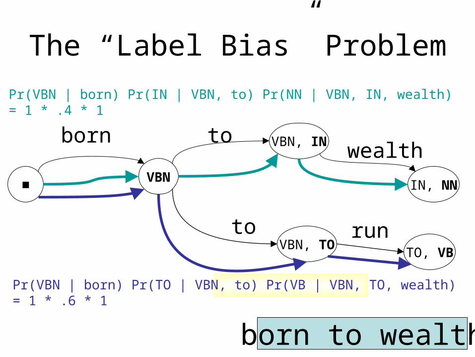
The “Label Bias” Problem
■VBN
VBN, IN
IN, NN
VBN, TO
born
to
towealth
run
born to wealth
Pr(VBN | born) Pr(IN | VBN, to) Pr(NN | VBN, IN, wealth) = 1 * .4 * 1
Pr(VBN | born) Pr(TO | VBN, to) Pr(VB | VBN, TO, wealth) = 1 * .6 * 1
TO, VB
Is this symptomati
c of log-linear
models?No!
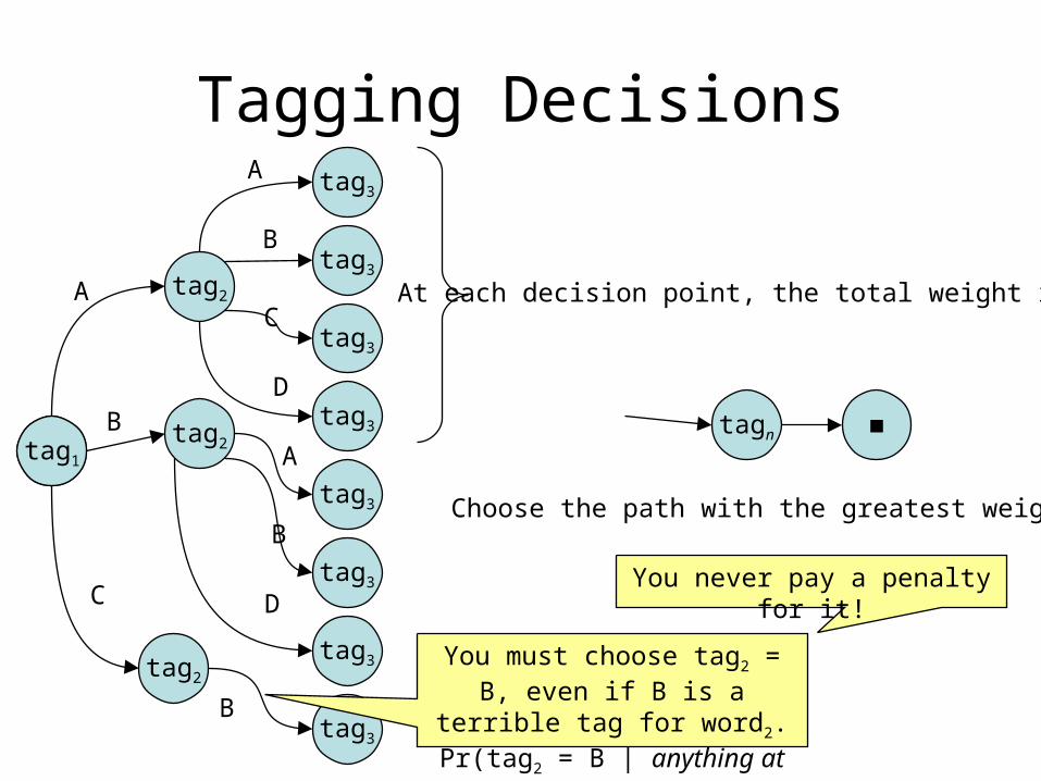
Tagging Decisions
tag1tag1
tag2
tag2
tag2
tag3
tag3
tag3
tag3
tag3
tag3
tag3
At each decision point, the total weight is 1.
tagn
Choose the path with the greatest weight.
tag3
A
B
C
A
B
C
D
A
B
D
B
You must choose tag2 = B, even if B is a terrible tag
for word2.Pr(tag2 = B | anything at
all!) = 1
■
You never pay a penalty for it!
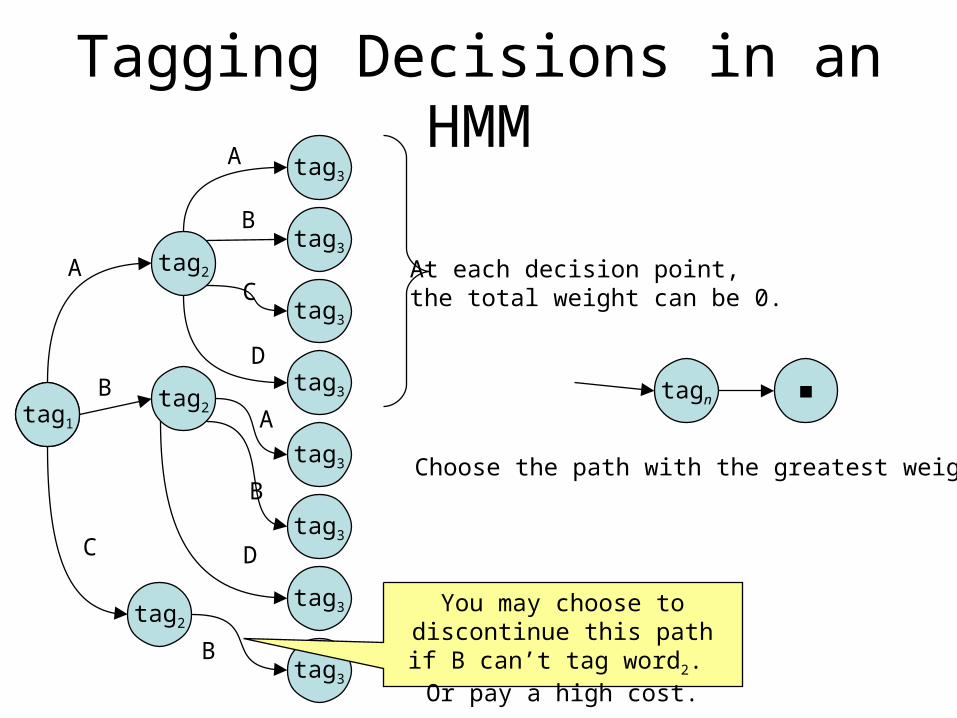
Tagging Decisions in an HMM
tag1tag1
tag2
tag2
tag2
tag3
tag3
tag3
tag3
tag3
tag3
tag3
At each decision point, the total weight can be 0.
tagn
Choose the path with the greatest weight.
tag3
A
B
C
A
B
C
D
A
B
D
B
You may choose to discontinue this path if B can’t tag word2. Or pay a
high cost.
■
Outline
Maximum Entropy principleLog-linear modelsConditional modeling for
classificationRatnaparkhi’s tagger Conditional random fieldsSmoothingFeature Selection
Conditional Random Fields
• Lafferty, McCallum, and Pereira (2001)
• Whole sentence model with local features:
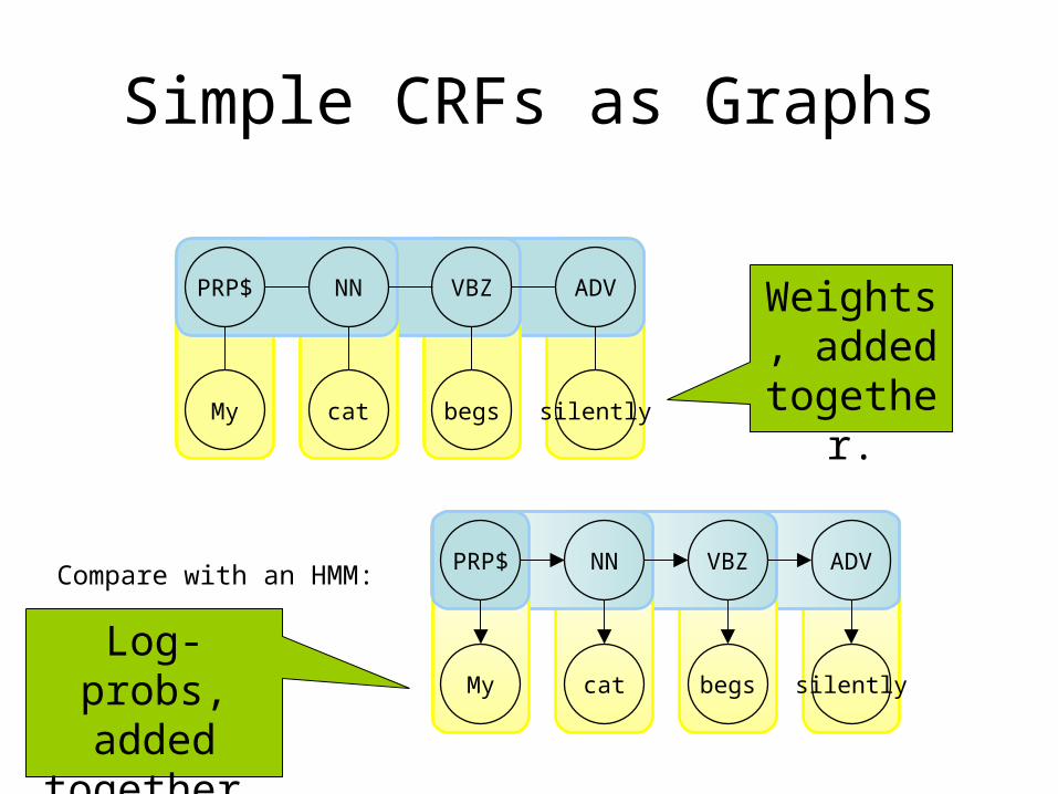
Simple CRFs as Graphs
PRP$ NN VBZ ADV
My cat begs silently
PRP$ NN VBZ ADV
My cat begs silently
Compare with an HMM:
Weights, added together
.
Log-probs, added
together.
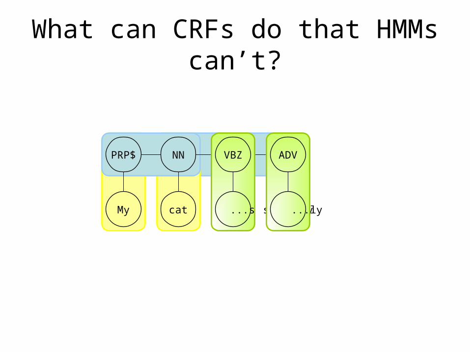
What can CRFs do that HMMs can’t?
PRP$ NN VBZ ADV
My cat begs silently
ADV
...ly
VBZ
...s
An Algorithmic Connection
What is the partition function?
Total weight of all paths.
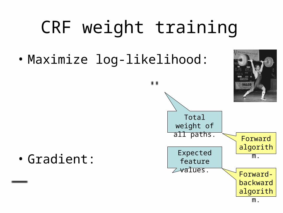
CRF weight training
• Maximize log-likelihood:
• Gradient:
Total weight of all paths.
Forward algorith
m.Expected feature values.
Forward-backwar
d algorith
m.
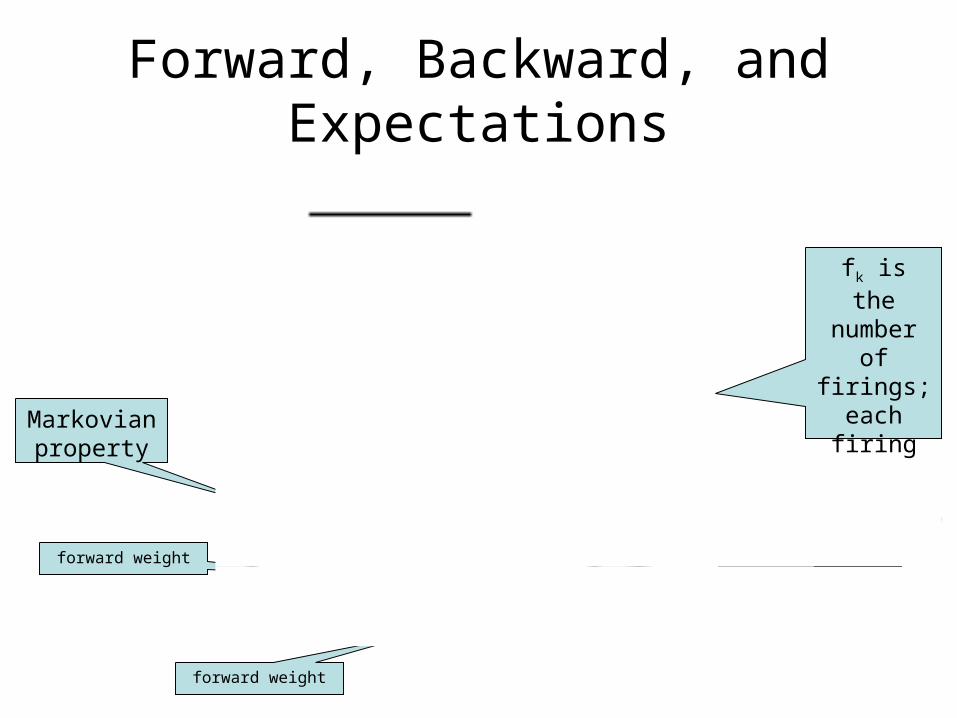
Forward, Backward, and Expectations
fk is the number
of firings; each
firing is at some position
Markovian property
forward weight backward weight
forward weight
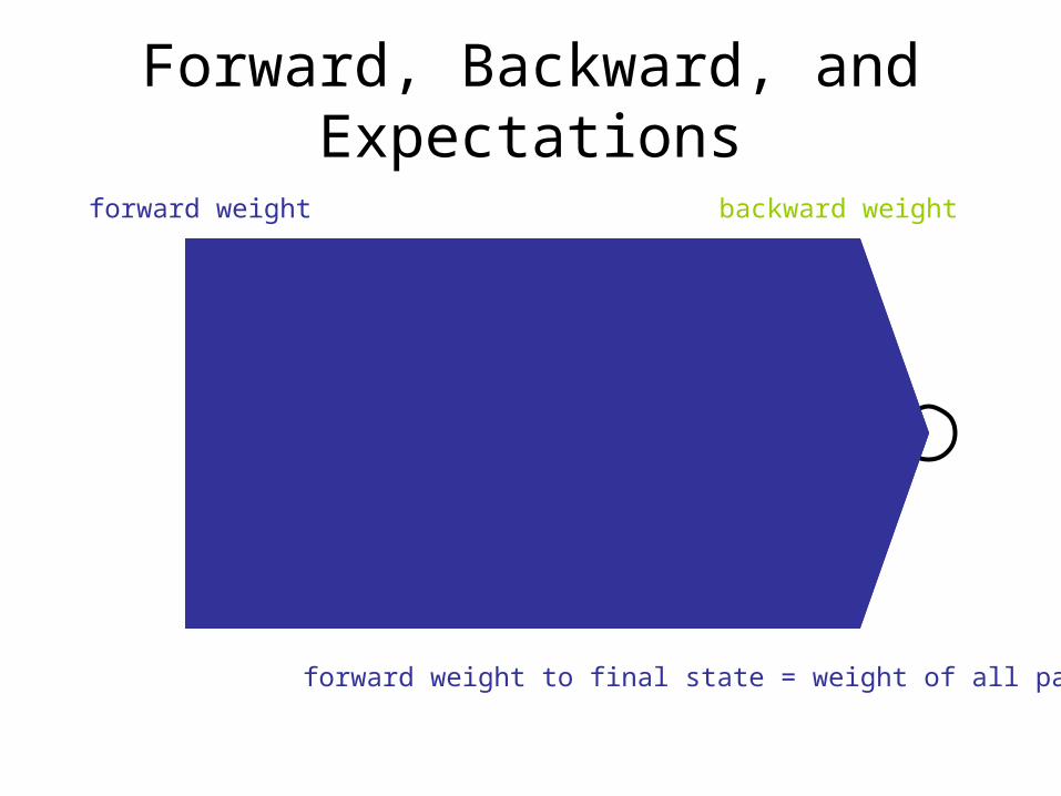
Forward, Backward, and Expectations
forward weight backward weight
forward weight to final state = weight of all paths
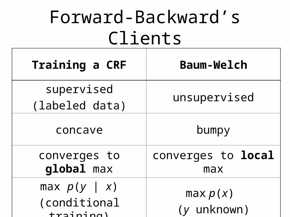
Forward-Backward’s Clients
Training a CRF Baum-Welch
supervised(labeled data)
unsupervised
concave bumpy
converges to global max
converges to local max
max p(y | x)(conditional training)
max p(x) (y unknown)
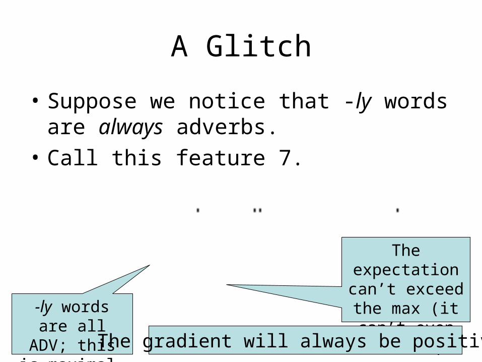
A Glitch
• Suppose we notice that -ly words are always adverbs.
• Call this feature 7.
-ly words are all ADV; this is maximal.
The expectation can’t exceed the max (it can’t even reach it).The gradient will always be positive.
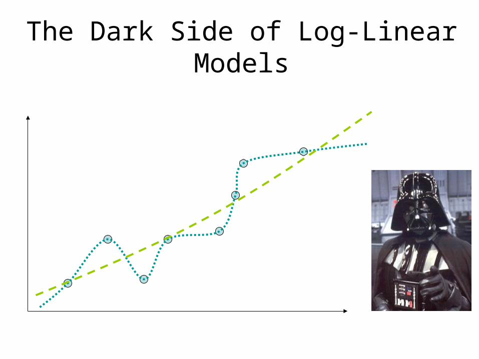
The Dark Side of Log-Linear Models
Outline
Maximum Entropy principleLog-linear modelsConditional modeling for
classificationRatnaparkhi’s tagger Conditional random fieldsSmoothingFeature Selection
Regularization
• θs shouldn’t have huge magnitudes• Model must generalize to test data
• Example: quadratic penalty
Bayesian Regularization:Maximum A Posteriori
Estimation
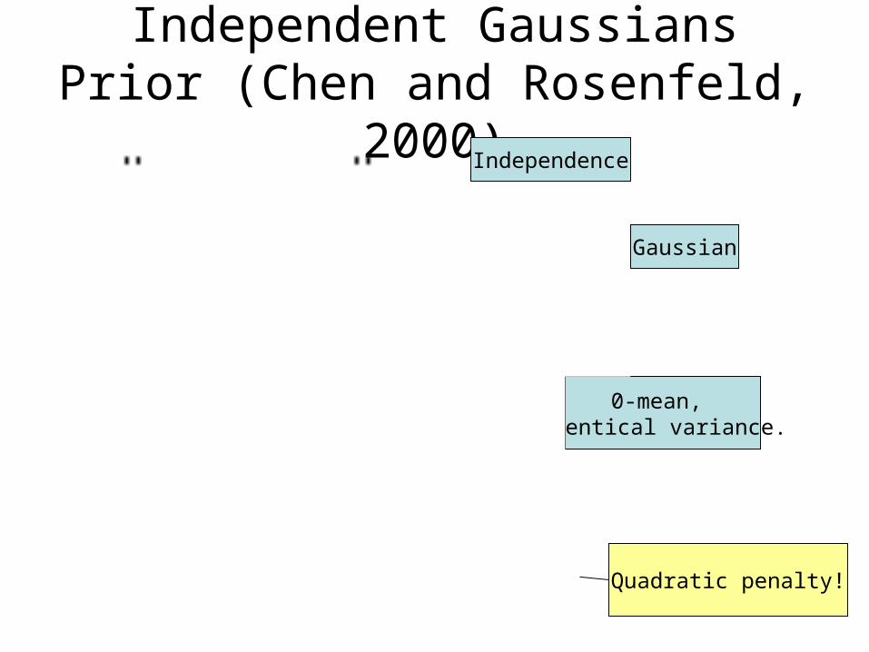
Independent Gaussians Prior (Chen and Rosenfeld, 2000)
Independence
Gaussian
0-mean, identical variance.
Quadratic penalty!
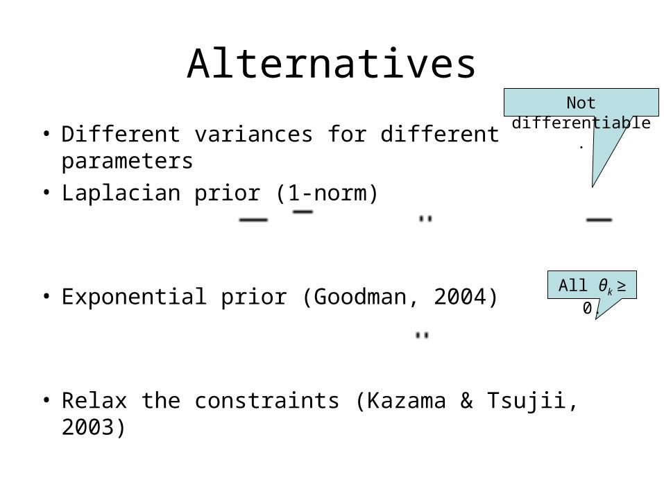
Alternatives
• Different variances for different parameters• Laplacian prior (1-norm)
• Exponential prior (Goodman, 2004)
• Relax the constraints (Kazama & Tsujii, 2003)
All θk ≥ 0.
Not differentiable.
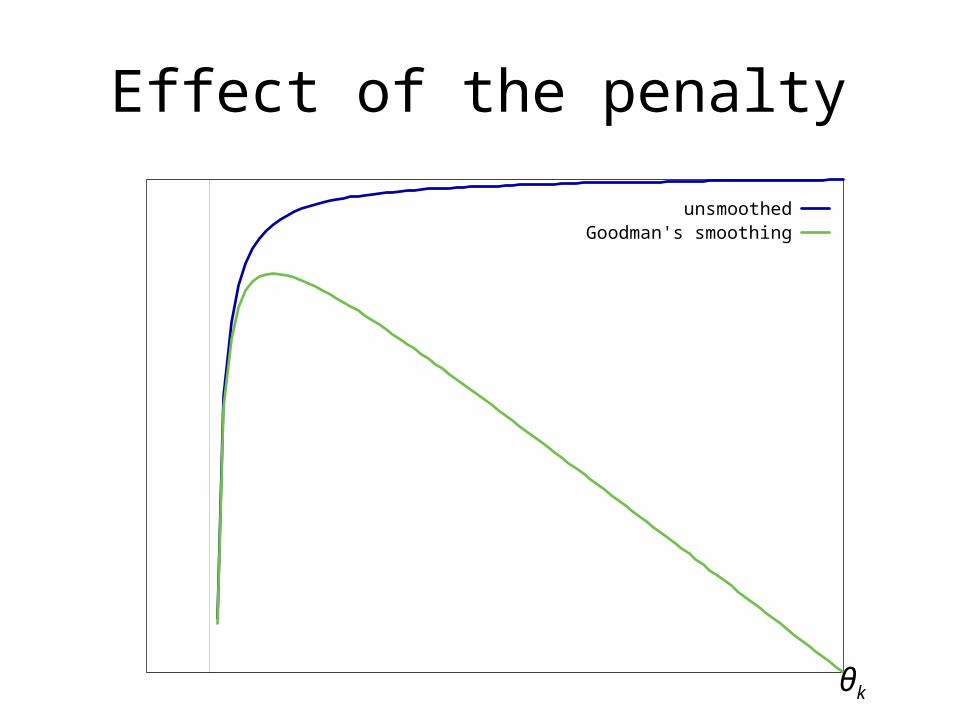
Effect of the penalty
unsmoothedGoodman's smoothing
θk
Kazama & Tsujii’s box constraints
The primal Max Ent problem:
Sparsity
• Fewer features → better generalization
• E.g., support vector machines
• Kazama & Tsujii’s prior, and Goodman’s, give sparsity.
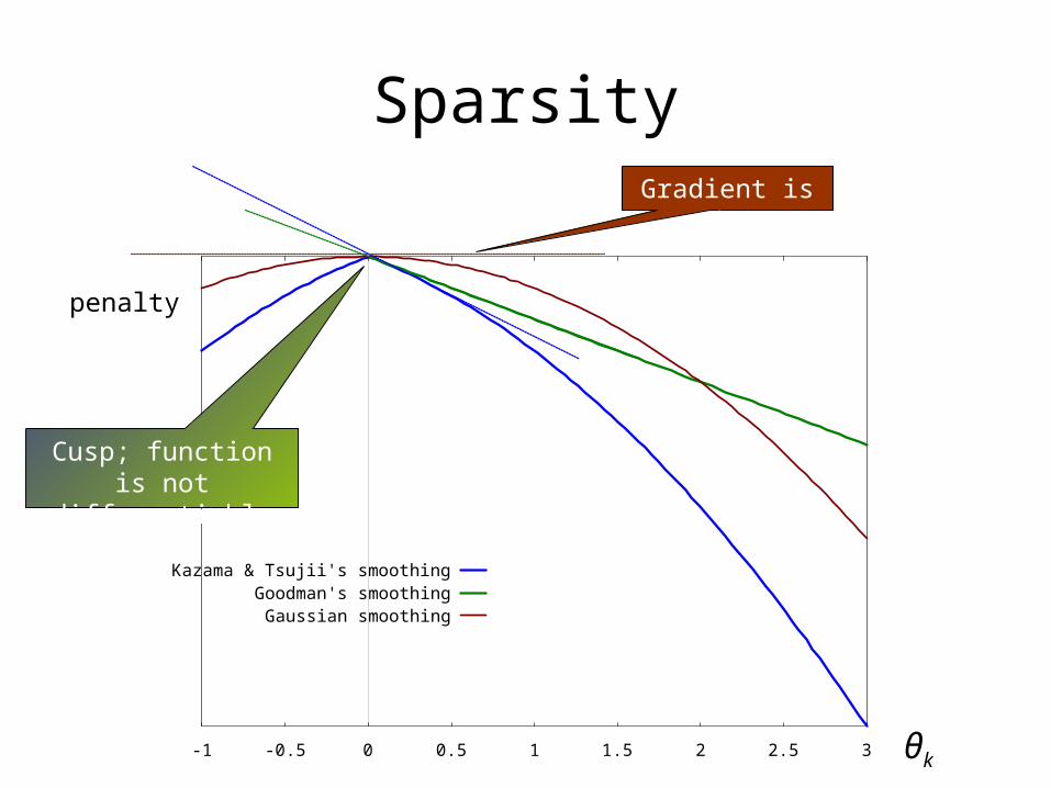
Sparsity
-1 -0.5 0 0.5 1 1.5 2 2.5 3
Kazama & Tsujii's smoothingGoodman's smoothing
Gaussian smoothing
θk
penalty
Cusp; function is not differentiable
here.
Gradient is 0.
Outline
Maximum Entropy principleLog-linear modelsConditional modeling for
classificationRatnaparkhi’s tagger Conditional random fieldsSmoothingFeature Selection
Feature Selection
• Sparsity from priors is one way to pick the features. (Maybe not a good way.)
• Della Pietra, Della Pietra, and Lafferty (1997) gave another way.
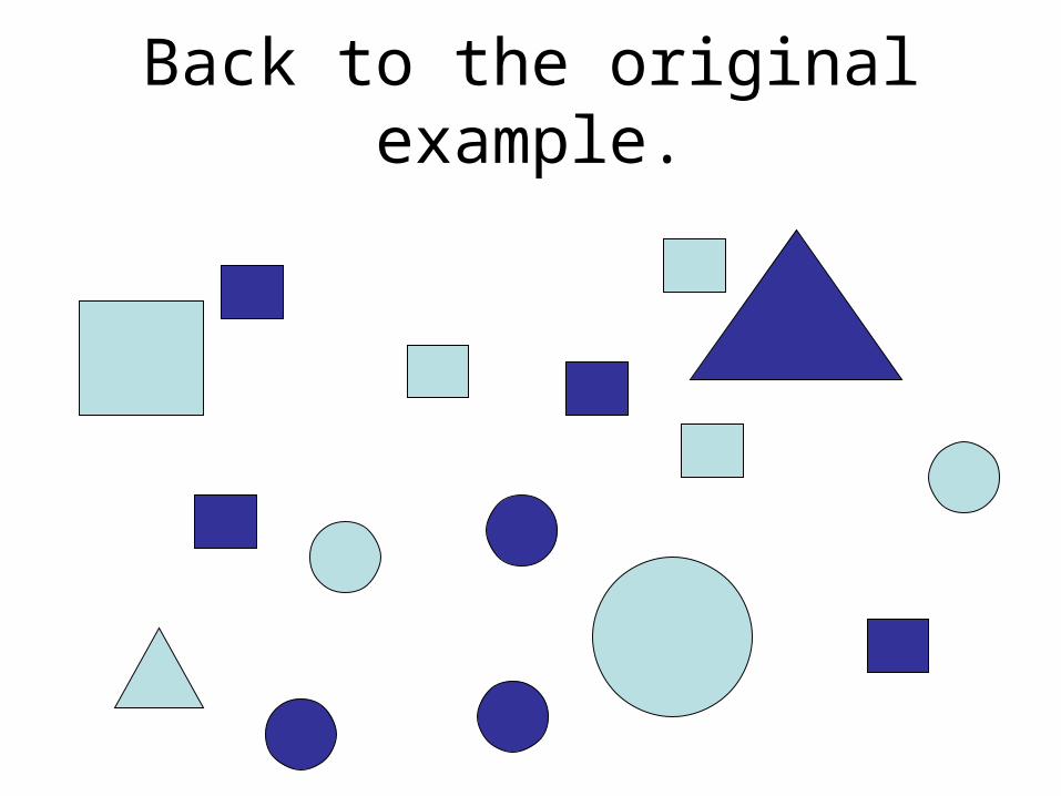
Back to the original example.
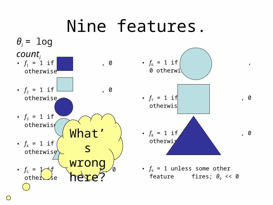
Nine features.
• f1 = 1 if , 0 otherwise
• f2 = 1 if , 0 otherwise
• f3 = 1 if , 0 otherwise
• f4 = 1 if , 0 otherwise
• f5 = 1 if , 0 otherwise
• f6 = 1 if , 0 otherwise
• f7 = 1 if , 0 otherwise
• f8 = 1 if , 0 otherwise
• f9 = 1 unless some other feature fires; θ9 << 0
What’s
wrong
here?
θi = log counti
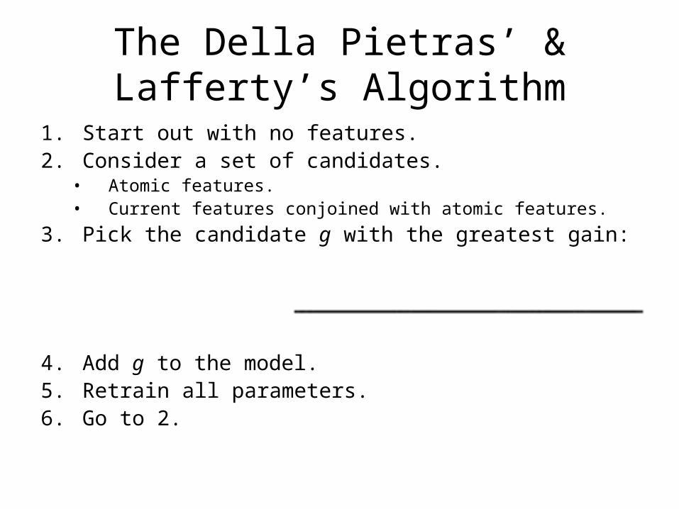
The Della Pietras’ & Lafferty’s Algorithm
1. Start out with no features.2. Consider a set of candidates.
• Atomic features.• Current features conjoined with atomic features.
3. Pick the candidate g with the greatest gain:
4. Add g to the model.5. Retrain all parameters.6. Go to 2.
PRP$
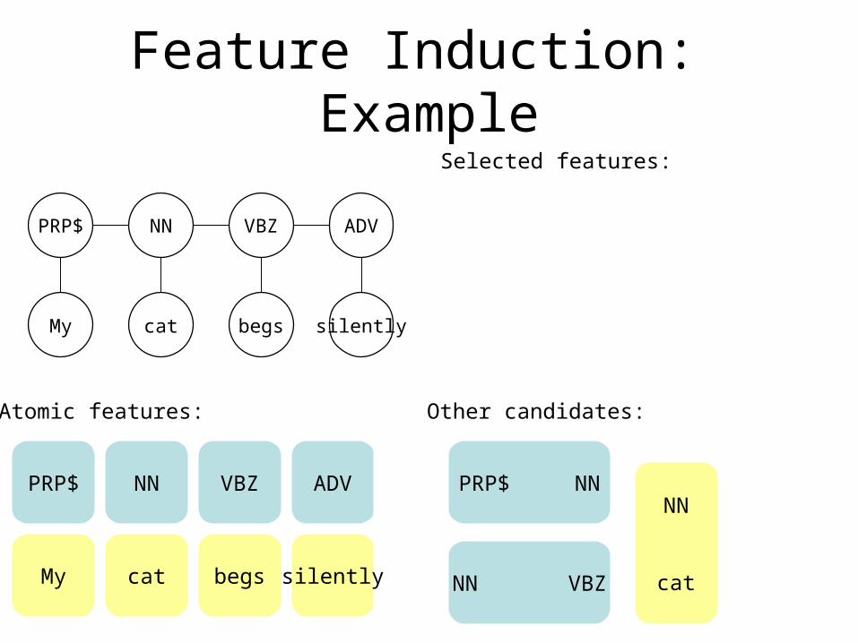
Feature Induction: Example
PRP$ NN VBZ ADV
My cat begs silently
Atomic features:
NN VBZ ADV
My cat begs silently
Selected features:
Other candidates:
NN VBZ
PRP$ NNNN
cat
Outline
Maximum Entropy principleLog-linear modelsConditional modeling for
classificationRatnaparkhi’s tagger Conditional random fieldsSmoothingFeature Selection
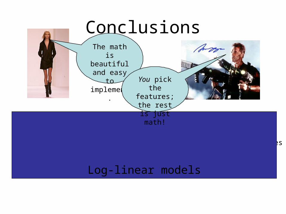
Conclusions
Probabilistic models:robustness
data-orientedmathematically understood
Hacks:explanatory power
exploit expert’s choice of features(can be) more data-oriented
Log-linear models
The math is beautiful and easy
to implement. You pick
the features; the rest is just math!

Thank you!