Load-Based Licensing: Getting the rates right†

Tiho Ancev* and Regina Betz** Abstract Load-based licensing is a form of pollution taxation that has been recently adopted for various air and water pollutants in New South Walles. As with other taxation based systems for pollution control, the effectiveness of load-based licensing depends on the levels of the set marginal fee rates and the responsiveness of the abatement activities by the polluters to those rates. After four years of the load-based licensing system in NSW, whereby the marginal fee rates gradually increased, data were available to conduct testing as to the effects of the changes in the marginal fee rates on the level and on the changes of NOx emissions by licensed emitters. Analysis was conducted using econometric methods suitable for panel data analysis. Results from the conducted analysis suggests that overall, the marginal fee rates were probably set too low to warrant substantial reduction in NOx emissions. This finding calls for modification of the existing system by increasing the load-based fee rates, perhaps in combination with a system of tax revenue recycling, along the lines of the Swedish NOx system. An alternative that warrants serious consideration is a tradable permit system for NOx as implemented in some parts of the US. JEL classification: Q52, Q53, Q58. Keywords: abatement, emission fees, load-based licensing, nitrous oxides (NOx). † The authors would like to acknowledge the assistance by Vo Ha Trang, Johanna Cludius, and Ioana Oprea in data analysis. The help obtained from the Department of Environment and Conservation, NSW in relation to data access and interpretation is gratefully acknowledged. Authors would also like to thank Tony Owen for valuable comments on earlier versions of the paper. * Discipline of Agricultural and Resource Economics (A04), University of Sydney, t.ancev@usyd.edu.au ** School of Economics and Centre for Energy and Environmental Markets, University of New South Wales, r.betz@unsw.edu.au

1

Load-Based Licensing: Getting the rates right Introduction Load-Based licensing is a relatively novel application of Pigouvain pollution fees where a

given installation is liable to pay pollution emission fees that are assessed based on the

quantity of emissions, the marginal fee rate, the noxiousness of the pollutant, and the

location of the installation. This system of load based fees has several advantages over

the conventional approaches to regulating emissions, and provides more flexibility for

emitters. They are left with the choice to either pay the fee or to invest in abatement

technology and reduce the amount of emissions.

In New South Wales, a system of load-based licensing has been in place since

1999. This system was introduced by the Protection of the Environment Operations

(General) Regulation 1998. Among other pollutants, the scheme covers nitrous oxides

(NOx). The system was introduced gradually, and one of the elements that comprises the

payable fee formula, the "pollutant fee unit value" was incrementally increased every

year from zero in 2000 to $35 in 2003, a level at which it remains at present. This gradual

rise in the rate of the pollutant fee, which in essence represents a Pigouvian tax on NOx

emissions, allows researchers to observe four different levels of fee rates in four years. It

is theoretically expected that as the rate of the fee increases, more abatement should take

place and hence emissions should be reduced. Observing the behavior of the regulated

industries in relation to their emissions under this system of load based taxation, can in

principle provide us with some insight as to their abatement intensity and costs, and the

ex-post effectiveness of the set fee rates given those characteristics of abatement.

2

From the regulatory perspective, the main concern is that if the rates are set too

low, the effectiveness of the load-based scheme in reducing emissions would be limited.

Emitters, finding it cheaper to pay the fee, would do so rather than abate more. Thus, with

fees set too low, the load-based licensing system would not be addressing the problem

that it was designed to address in the first place − reducing pollution emissions.

After having the load-based licensing system for NOx in NSW in place for some

time, data are now available to conduct testing on whether the marginal fee rates reflected

in the load-based fee formula have been set at least approximately effectively, and

whether the scheme has in fact resulted in reduced emissions. The aim of the paper is to

empirically test the hypothesis that the marginal fee rates implemented under the load-

based licensing scheme for NOx in NSW have been effective in reducing NOx emissions.

Based on the results obtained from this study, policy recommendations can be put

forward and the rates can be reassessed and adjusted.

The economics of load-based licensing has not been extensively studied in the

literature. The adoption of the scheme in NSW, has been predated by government

department studies with some economics content (EPA NSW, 1999). Taxation of air

pollutants, and in particular NOx emissions, which are of main interest in the current

paper, has been empirically surveyed in a predominantly European context by Cansier

and Krum (1996). Also, the French air pollution system and its effectiveness have been

analyzed by Millock and Nauges (2003) in an empirical setup that is similar to the one

presented in the current paper. A body of literature that relates emissions to physical

output and treats the system of tax revenue recycling has been pioneered by Fisher (2001)

and Sterner and Höglund (2000). Abatement costs functions for NOx from energy

3

production in three industrial sectors have been analyzed in a recent paper by Höglund

(2005). The data used in the study were based on the Swedish tax revenue recycling

system and showed that a number of relatively inexpensive abatement cost options are

available in these industries (e.g. optimization of combustion processes). In addition,

substantial published work assessed RECLAIM, the NOx trading system in California

(Foster and Hahn 1995; Fromm and Hansjürgens 1996).

The article is structured as follows. In the next section we outline a theoretical

discussion that underlies the ensuing empirical analysis of load-based licensing.

Following is a section where we describe the data that were used in the empirical study.

This is followed by description of the methods used. The results from the empirical study

are reported in the penultimate section, together with a discussion. The ultimate section

provides a summary and discusses policy implications.

Theory

Since Pigou (1920), economists have contended that an efficient tax on emissions for an

individual emitter will equate the tax rate with the cost of reducing the emissions at the

margin. The emitter will find it advantageous to abate emissions as long as the abatement

activity is less costly than paying a tax at the marginal rate. Once it becomes more

expensive to abate, the tax will be paid. Conceptually then, under an emission tax regime,

a pollutant emitting firm will maximize profits:

(1) teeycpyey

−−=Π ),(max,

,

where p is the exogenous price for the firm’s product y, c is a cost function, e is the

quantity of emissions and t is the marginal tax rate. From the first order conditions

4

pertaining to the above optimization problem one can derive the familiar expressions that

price equals marginal cost of production p = cy, and that the costs of abatement are equal

at the margin to the tax rate –ce = t , where subscripts denote partial derivatives.

This basic model should hold true in the case of load-based licensing after care

has been taken of the particularities. The key modification is the way the payable load-

based fee is calculated. The following formula is used in a load-based licensing scheme:

(2) 10000

w we t P SPF =

where PF denotes the payable pollution fee, e denotes the quantity of emissions of a

particular pollutant, t is the fee rate, Pw is a pollutant weighting according to the

noxiousness of the pollutant, and Sw is a spatial weighting, which puts heavier weight on

the installations that are located in “critical” zones where environmental damages are

perceived to be more severe1. In the light of the load based licensing formula, the

standard representation of equation 1 suggests that under a regime of increasing fee rates

(marginal tax rates), it is theoretically expected that more abatement will be undertaken

and emissions reduced. If this is not empirically observed, then it will be an indication

that the marginal fee rates were perhaps set at a too low level and did not provide

sufficient incentive for the emitters to engage in substantial abatement. To conduct an

empirical study and to be able to test whether the marginal rates of the load-based fees

have been set correctly, one would aim at relating the emissions of pollution to the level

of produced output, the components of the load-based fee formula, including the varying

tax rates, and potentially some industry or firm specific characteristic.

1 This representation of payable fee formula is in a general form. The formula can have another form dependent on the “fee rate threshold”. This is discussed in greater detail in the “Data” section of the article.

5

To conceptualize this, some modifications to the representation of equation 1 are

needed. We begin with the firm’s profit maximization problem2:

(3) ,

max ( , ) w wepy c e etP SΠ = − −

xx ,

where y = f(x) and e = g(y). y is the physical output, x is a vector of inputs, and e, t, Pw

and Sw are components of the load-based licensing formula as defined above. This relates

the emissions to both the level of input use x, as well as to the particular production

technology . The first order condition with respect to emissions result in the familiar

finding that cost of abatement should equal the tax rate at the margin. The first order

condition with respect to the input use is:

( )•f

(4) 0w wy c e yp tP Sx x y x

⎡ ⎤∂ ∂ ∂ ∂− − =⎢ ⎥∂ ∂ ∂ ∂⎣ ⎦

.

This can be manipulated by dividing through by xy ∂∂ / :

(5) 0w wc x ep tP Sx y y∂ ∂ ∂

− − =∂ ∂ ∂

,

and

(6) w we ctP S py x

xy

∂ ∂ ∂= −

∂ ∂ ∂.

This allows us to express the change in emissions as the level of produced output changes

by:

(7) w w

c xpe x yy tP S

∂ ∂−

∂ ∂ ∂=∂

.

2 We drop the denominator of 10,000 here for notational simplicity. It may be assumed that the either the emissions or the tax rate are expressed as a ratio to 10,000.

6

This suggests that in a general form, the emissions of a pollutant can be expressed as a

function of the output produced, its price and the cost of production, as well as the

marginal tax rate, pollutant weighting and spatial weighting:

e dyy∂

=∂∫ e = ψ (y, p, c, t, Pw, Sw). Taking a ratio of emissions to output e/y = E, we can

restate the above expression as E = ψ(p, c, t, Pw, Sw). Here, we would like to evaluate the

following3: and w

ES t∆ ∆∆ ∆

E . We are particularly interested in the last one —the effect of

the changes in marginal fee rate on the emission of pollutants. This can be measured by

the elasticity of emissions with respect to the fee rate: E tt E

∆∆

.

The theoretical relationship between the quantity of emissions and the fee rate

will depend on the possibilities for abatement that are at disposal to the emitting

installations. When the abatement has to be achieved by a substantial investment in new

end-of-pipe abatement technology it is expected that the emissions will be less responsive

to the initial implementation of the load based fees, as a result of a large, lumpy nature of

the abatement investment required (McKitrick, 1999) and inertia. On the other hand, if

there are technical possibilities to achieve emission reductions without such large

investment, by optimizing the combustion process and exploiting abatement options

within the system, it is expected that emission abatement achieved in this manner would

be fairly responsive to implementation of increasing load fees.4

3 The pollutant weighting was constant during the sample period, with a value of 6. It has recently increased to 9, but the data reflecting this change are not yet available. Therefore the changes in pollutant weighting are not treated further in this analysis, but are of imminent research interest. 4 NOx emissions abatement options range from energy saving measures or trimming the combustion process up to end-of- pipe technologies such as Flue Gas Desulphurization or Selective Catalytic Reduction. The latter is able to reduce emissions substantially but with substantial costs, www.pollutionengineering.com/CDA/ArticleInformation/coverstory/BNPCoverStoryItem/0,6646,107005

7

In addition to this, it seems that installations in NSW have a choice of

implementing either a continuous emission monitoring system (CEMS) or periodic

monitoring. While continuous monitoring offers a possibility for verification of

abatement achieved through optimising the combustion process, periodic monitoring is

not conducive to such verification. This may reduce the incentives for the installations to

adopt these relatively low cost abatement options (Sterner, 2003). We were not able to

collect data on the type of monitoring across the installations in NSW covered in the data

sample, but some anecdotal evidence suggests that the periodic monitoring is

predominant.

In relation to the levels of fee rates, it is expected that when they are set at a low

level and the end-of-pipe technology is the only available abatement option, the changes

in emissions as the fee rates are marginally increased are not going to be substantial. In

this case, the cost of paying the fee is likely to be smaller than the cost of the equivalent

abatement by any end-of pipe technology which involves substantial investment.

However, as the fee rate is increased it is expected that the incentives to reduce emissions

on the part of the emitters become greater.

Data

Data were obtained from the Department of Environment and Conservation, NSW. The

data set consisted of information on NOx emissions and physical output for seventy-five

installations that are licensed to emit NOx in NSW. The observations were for the years

2000, 2001, 2002, and 2003. The corresponding marginal rates for the pollutant fee unit

value for NOx were $0, $24, $29 and $35 for these years, respectively.

8

For each installation in the data set, the payable fee is based on the "assessable

load" of the pollutant in kilograms of NOx per year. This load may represent the actual

emissions monitored on the basis of standardized protocols, or it may be a value agreed

between the government and the emitter based on various criteria (Clause 18, Protection

of the Environment Operations (General) Regulation 1998). These criteria are not treated

in this paper, and the assessable load is taken at “a face value”. This assessable load is

multiplied by the pollutant weighting (Pw) for NOx, which was 6 for the period covered

in the data set (2000-2003), but has recently increased to 9. The assessable load is further

multiplied by the spatial weighting (Sw) based on the critical zone where the installation is

located.5 All of this is then multiplied by the marginal fee rate for the appropriate year (0

for 2000, $24 for 2001, $29 for 2002 and $35 for 2003), and divided by 10,000.

An alternative formulation of the payable load-based fee has been used when the

assessable load is above the fee rate threshold (FRT). The FRT is determined based on

the FRT factor, which varies according to activity classification so that the FRT factor for

NOx would be very different between industries.6 The threshold is obtained by

multiplying this factor with the output quantity for a given installation. If the assessable

load is greater than this fee rate threshold, then the operator has to pay double the fee for

5 For the following areas the critical zone weighting of 7 applies: Ashfield, Auburn, Bankstown, Baulkham Hills, Blacktown, Blue Mountains, Botany, Burwood, Camden, Campbelltown, Canterbury, Concord, Drummoyne, Fairfield, Hawkesbury, Holroyd, Hornsby, Hunters Hill, Hurstville, Kiama, Kogarah, Ku-ring-gai, Lane Cove, Leichhardt, Liverpool, Manly, Marrickville, Mosman, North Sydney, Parramatta, Penrith, Pittwater, Randwick, Rockdale, Ryde, Shellharbour, South Sydney, Strathfield, Sutherland Shire, Sydney, Warringah, Waverley, Willoughby, Wollongong, Woollahra. The critical zone weighting of 2 applies for the following areas: Cessnock, Gosford, Lake Macquarie, Maitland, Muswellbrook, Newcastle, Port Stephens, Singleton, Wollondilly, Wyong. For all other areas in NSW a critical zone weighting of 1 applies. 6 For example electricity industry has an FRT factor of 2,700 which only applies to installations with a capacity to generate more than 250 GWh per annum. For refineries the FRT factor is 0.5 and applies to refineries with more than 100 t output per year (see Schedule 1 in POEO(General) Reg).

9

emissions above the threshold. The formula used in the calculations of the payable load-

based fee can be represented as:

(8) /10000

(2 ) /10000

w w

w w

etP S if e FRTPF

e FRT tP S if e FRT

<⎧⎪= ⎨⎪ − >⎩

Based on these variables, the panel that the data formed was highly unbalanced,

with records for some installations only covering one or two years. In response to this, a

criterion of at least three time series records per cross-section (i.e. for each installation,

records for at least three of the above four years were required for this installation to be

included in the data set) was established. Only data on installations that satisfied this

criterion were included in the refined data set. Data were further inspected visually and

by plotting, which was followed by filtering erroneous records out of the data set. This

resulted with data for 65 installations remaining in the sample.

Even after this filtering the panel was still unbalanced with records for 14

installations only covering a period of three years. Moreover, the missing year was not

the same for all of these 14 installations, being either the first year in the sample (2000)

or the last year in the sample (2003). This amounts to having contiguous observations

over time for all cross-sections, albeit of various length and various starting and ending

points. The total number of data points in the set was 246.

Spatial weightings for each individual installation were also included in the data

set according to the regulatory requirements. The weightings had values of 7, 2 and 1,

dependent on the location of the installation (see footnote 3). Forty installations included

in the data set were in fact located in the critical zone with weighting of 7, fifteen in

critical zone with weighting 2, and ten installations in critical zone with weighting 1.

10

Individual installations were grouped according to the industries to which they

belonged. The sixteen industry groupings in alphabetic order were: Agricultural

fertilizers, Biomedical waste incineration, Cement or lime production, Ceramics

production, Coke production, Electricity generation, Glass production, Paper production,

Paint production, Petroleum refining, Plastics production, Primary aluminum production,

Primary iron and steel production, Secondary aluminum production, Secondary iron and

steel production, and Other secondary non-ferrous alloys production.

Individual installations were also classified by their size in terms of emission of

NOx based on the assessable load. The cutoff point was established at 200,000 kg of

NOx emitted per annum. A binary variable was then created, with a value of unity for the

installations with emissions greater than this cutoff, and a value of zero for installations

with emissions lower than this cutoff. The resulting distribution was approximately one

third of installations being classified as large emitters and two thirds as smaller emitters.

An additional binary variable was formed reflecting the formula used to calculate

the paid fee according to equation 8. The value of this variable was zero if the emissions

were lower than the fee rate threshold and unity otherwise. There were 26 occurrences

where this variable had a value of 1, across nine installations.

Pooling the data for all facilities and all industries together gives a broad picture

about the dynamics of the physical output and NOx emissions under the increasing fee

rates. This is presented in Table 1. The information displayed in the table suggests that

over the four years in which the load fees gradually increased from $0 to $35, the

aggregate emissions of NOx from the installations included in the sample initially

increased but than decreased. In the same time, the aggregate physical output from these

11

installations increased by about one third. This suggests that there has been some

reduction of NOx emissions per unit of output in NSW over the sample period.

Moreover, apparent in Table 1 is the relationship between the physical output and NOx

emissions. At the time of the first increase in the rate of load fee from zero to $24, the

physical output grew very strongly (almost 44%, and this was the year of the Sydney

Olympics) and the NOx emissions consequently followed suit. As the growth in physical

output settled down in the following years, the emissions also dropped significantly,

going below the initial level. This relationship between the physical output and emissions

is visually presented with a plot in Figure 1.

Table 1 also displays the total and average fees paid over the sample period. The

average fee paid across all installations was $33 per ton of NOx, $37 per tNOx and $46

per ton of NOx in 2001, 2002 and 2003 respectively, which is considerably lower than

comparable figures paid under the RECLAIM program in the US, or under the Swedish

NOx tax system.

Both Table 1 and Figure 1 indicate that there has been some abatement of NOx

taking place in the installations covered in the sample. As presented in the theory section,

the expectations are that this is due to the increasing fee rates. However, this has yet to be

proved in an empirical setting. To that end, for each observed data point (i.e. a cross

section − time series entry) we have taken the ratio of emissions to physical output,

effectively representing the amount of emissions per unit of output, which is consistent

with the discussion in the theory section above. This has two effects. Firstly, it eliminates

the potential need for weighing individual facilities according to their emissions, since

some emit many times more than the others. Secondly, it eliminates the effects that

12

variation in output has on the variation in emissions. In some instances a natural

logarithm of this newly created variable was a dependent variable, and in other instances

the first difference of the same variable was a dependent variable. In the ensuing

econometric analysis they were regressed against a set of explanatory variables, based on

the theoretical expectations discussed above.

Method

Given the available data and the aims of the research, an econometric study was

conducted in an attempt to isolate the effects of individual variables on the NOx

emissions per unit of output. The data were in an unbalanced panel format where for each

installation (cross-section) there were observations for either three or four years. Several

models were estimated using maximum likelihood estimation in SAS® (Proc Mixed). The

semi-log functional form was chosen for the model where the dependent variable was the

natural logarithm of the ratio of NOx emissions to output. This functional form

corresponds well with the theoretical expectations and has straightforward interpretation.

Since the key relationship of interest was how emissions per unit of output relate

to the increasing fee rates, the simplest model – the pooled estimator – was initially used

to get a feeling about the strength and the direction of the relationship (Johnston and

DiNardo, 2002). This model was of the form:

(9) 0 1ln E tβ β ε= + + ,

where E represents emissions per unit of output, t is the fee rate, β0 and β1 are coefficients

to be estimated and ε is a normally distributed random error term.

13

Even though this model in essence ignores the panel data structure and is therefore

inappropriate, it should still capture a strong correlation between the variables if such

correlation exists. Surprisingly in this case, the estimate for β1 was negative, but

insignificant, suggesting that the relationship between the fee rate and NOx emissions per

unit of output is not strong.

Next, a model was tested that included all the variables specified previously. For

this model, an individual intercept was estimated for each industry. In addition to the fee

rate variable, it also included the critical zone and the fee rate threshold variables.

Interaction terms between these variables and the fee rate were also tested, but were

found insignificant. Groupwise heteroscedasticity was suspected for observations for

large emitters (emissions greater than 200,000 kg NOx per year) and observations for

smaller emitters (emissions less than 200,000 kg NOx per year), so that the variance of

the error term may not be constant across smaller and larger emmiters. A test for

heteroscedasticity was conducted. This was done by estimating a model and outputting

the residuals, which were subsequently regressed on the “size” variable (binary variable,

being 0 for emissions less than 200,000 and 1 otherwise). The estimated coefficients were

significant, suggesting strong presence of groupwise hetereoscedasticity. This covariance

structure was taken into account in estimating a model of the following form:

(10) 15

0 1 2 3 41

ln k i i n ji j

E D t CZ FRT kβ β β β β=

= + + + + +∑ ∑ ε ,

where the kth observation on the natural logarithm of the emissions per unit of output

was a function of an industry specific intercept Di, the fee rate in a given year tn, the

critical zone weighting CZj (with j = 1 or 2, since j =7 was the base level) and the fee

rate threshold, FRT = 0 (since the FRT = 1 was the base level). Due to groupwise

14

heteroscedasticity the covariance structure of the error term was , where 20sizeσ = Ω

0

⎡ ⎤⎢

= ⎢⎢ ⎥⎣ ⎦

2size=

2size=1

1 0σΩ

10 σ

⎥⎥

1)

, and “size” is the variable pertaining to the emissions

above (or below) the determined cutoff of 200,000 kg NOx.

Estimating this model will produce results that can be used to make inferences

about the effects of each of the considered variables on the NOx emissions per unit of

output. However, we are interested here in explaining the change in NOx emissions (or

the lack of it) over the sample period, by looking at the effects that the considered

explanatory variables had on those changes. For this purpose, the first difference of the

ratio of emissions to output was taken. This was then regressed on the same set of

explanatory variables as in the previous model (i.e an industry specific intercept, the fee

rate, the critical zone weighting, and the fee rate threshold binary variable. The model

had the following form:

(11) , 15

, , 1 0 1 2 3 4 , (1

k n k n i i n j k n ni j

E E D t CZ FRTβ β β β β ε− − −=

− = + + + + +∑ ∑

where the variables were as defined above and the same covariance structure was used

due to presence of groupwise heteroscedasticity. A test for autocorrelation was also

conducted but did not indicate presence of autocorrelation.

Results

The results from the pooled estimator (equation 9) indicated poor data fit. Both the

intercept and the coefficient on the fee rate were insignificant. The estimate for the

coefficient on the fee rate was -0.0011 with a standard error of 0.2. This poor fit was also

15

indicated by the F-statistics for the fee rate ( a value of 0.08, with denominator d.f. 244)

The results for the model where natural logarithm of NOx emissions per unit of

output was a dependent variable (equation 10) indicate much better data fit. These results

are summarized in Table 2. The results suggest that apart from the fee rate, all other

variables are significant in explaining the NOx emissions per output for the installations

in the sample. This was strongly supported by the F test for joint significance. The results

indicate insignificance of the fee rate, which is counter to the theory presented in this

paper, and counter to intuition. This leads to an inference that the rates have probably

been set too low, and are not a major determinant of the patterns of NOx emissions under

the load-based licensing scheme in NSW. Other variables that are part of the formula

used to determine the payable fee, such as the spatial weighting (CZ) and the fee rate

threshold (FRT) are much more influential in explaining NOx emissions from

installations included in the sample. The coefficients on spatial weighting according to

critical zones (1, 2 or 7) indicate that installations located in the zone with weighting of 7

had lower emissions as compared to other zones. This result is expected, since the

formula for payable fee strongly penalizes emissions that are coming from installations in

urban areas, where the perceived damages (predominantly health effects) from NOx

emissions are much higher. Also large emitters, such as electricity generation plants tend

to be located outside urban areas for other obvious reasons (e.g. availability of coal

deposits).

Estimated coefficient for the fee rate threshold suggests that installations that had

at least one occurrence of emissions greater than the threshold were in essence emitting

more NOx compared to installations that were always below the threshold. As mentioned

16

above, an interaction term between the fee rate and the fee rate threshold was statistically

tested but was found insignificant.

Estimates of covariance parameters are significant indicating strong presence of

groupwise heterscedasticity based on whether the installation was classified as large

(more than 200,000 kg of NOx) or relatively smaller emitter (below that value). The

likelhoood ratio test of heteroscedasticity confirms its presence.

The results for the model where the first difference of the emissions per unit of

output was a dependent variable (equation 9) are reported in Table 3. Results indicate

very poor data fit, suggesting problems caused by autocorrelation. However, in addition

to testing for autocorrelation, which did not confirm its presence, an autoregressive

covariance structure was also tested, but the covariance parameters were found

insignificant. This has led us to work with the model as estimated and with results as

presented in Table 3.

Estimated coefficients on the explanatory variable were insignificant at the usual

significance levels for all variables. This suggests that the considered variables have not

influenced the changes in NOx emissions per unit of output in any recognizable manner.

The emissions have changed, and in fact as shown previously in Table 1, they have

reduced, but those reductions can not be explained by the variables that are part of the

load-based fee formula, including the changes in the marginal fee rates.

In addition, changes in emissions can not be explained by industry specific

intercepts. The results in Table 3 show that the industry specific intercept was significant

but positive for only one of the considered industries. This is the electricity generation

industry, which is by far the greatest emitter of NOx in NSW. This result suggests that

17

the members of this industry tended to increase the emissions per unit of output during

the sample period. Closer inspection of the data reveals interesting findings. The average

emissions per unit of output for the industry in fact declined from 2341.82 in 2000 to

2049.51 in 2001, to 1914.29 in 2002 to 1764.35 in 2003. However, this pattern of average

emissions was driven by substantial reduction of emissions in a single installation which

apparently invested in end-of-pipe abatement technology in 2000 and was able to reduce

its emissions per unit of output by about 3000 during the sample period. It is worthwhile

mentioning that this installation has started with rather high level of emissions per unit of

output and the reductions during the sample period has brought down their emissions to

be more in line with the industry average. This is indicative of a late adoption of end-of-

pipe technology that was earlier adopted by other members of the industry, which might

have been due to regulations for new plants.

Conclusion

Load-based licensing is a particular form of Pigouvian taxation of pollution that has been

operating in NSW since 1999. The interesting feature of this scheme is that the fee rates

have gradually increased in the period 2000-2003, from zero to $35. Based on economic

theory, and under the hypothesis that the fee rates have been chosen at least

approximately correctly, one would expect a significant reduction of emissions as the fee

rates increased. Data on NOx emissions and physical output across range of industries in

NSW are now available and were used to empirically test the theoretical expectations.

The variability of the fee rates over the period 2000-2003 allows for an empirical study

that relates emissions to those rates.

18

After some data manipulation, the sample included data on sixty five facilities

that emit NOx in NSW. The data covered the period 2000-2003 and were in a form of an

unbalanced panel. Individual facilities were classified in sixteen industries. Natural

logarithm, and the first difference, of the ratio of emissions to output were used as

dependent variable in several econometric models. The models were from a broad family

of panel data models, ranging from a simplest pool estimator, to the more complex

models with heteroscedastic covariance structure.

The results from the empirical study suggest that some reduction of NOx

emissions took place during the sample period. However, these reductions can not be

clearly attributed to the elements of the formula used to calculate the payable fees under

the load-based licensing scheme. This is an indication that fees were set at a too low

level. The effect of increasing fees was insignificant in explaining both the level and

changes of emissions per unit of output. While other elements of the formula for the

payable load-based licensing fee had significant explanatory power for the levels of

emissions per unit of output, this was not the case when the change in emissions per unit

of output was a dependant variable. An exception was an industry specific intercept for

the electricity industry, indicating that this industry, which is the largest emitter of NOx

in NSW did not respond significantly to the increasing load-based fee rates. This can be

probably explained with inflexible technologies and limited abatement options, but also

indicates a lack of economic incentives that the load-based licensing should have

provided.

Several conclusions can be drawn from this discussion. While the load-based

licensing has probably contributed toward reduction of the overall NOx emissions in

19

NSW in the sample period, it seems that those reductions are not in line with what would

be theoretically expected, provided the fee rates were set “correctly”. This suggests that

many facilities are finding it more advantageous to pay the fee than to abate. From a

regulatory perspective, if more abatement of NOx is aimed for, it seems inevitable to

further increase the fees. This might have been attempted by the recent increase in the

pollutant weighting for NOx from 6 to 9, which amounts to a 50% increase in the amount

of the payable fee and could therefore be interpreted as a 50% increase in the marginal

fee rate. While the results presented here show that the past increases in the fee rates in

the period 2000-2003 did not have a great impact on reduction of NOx emissions in

NSW, it is of imminent research interest to establish the effects of the most recent

increase in the payable load-based fees and whether it has been high enough to trigger

substantial NOx reductions.

It is suspected however that further increases might be necessary, since the

average fees for NOx paid in NSW are substantially lower than similar fees elsewhere.

For instance in Sweden, the average fees for NOx are set at levels almost 200 times

higher (around $7,240 per ton of NOx) than what was an average fee paid in NSW during

2000-2003.

These substantially higher fees may be paralleled with a tax revenue recycling

system, similar to the one operating in Sweden. To make the high emission fee levels

acceptable for the businesses, the tax revenues are returned to the polluting companies

relative to their output. Such a tax has been very successful in reducing NOx emissions.

Under this tax system, as Höglund (2005) has shown, there was a significant amount of

"low hanging fruits", or relatively inexpensive abatement options available to regulated

20

entities. This was in part due to the improved continuous-time monitoring equipment,

which provided an incentive for emitters to explore reductions by trimming, optimization

of combustion process, and operational adjustments. Greater use of continuous-time

monitoring of emissions in NSW could potentially deliver similar results.

Load-based licensing has several desirable characteristics relative to the more

standard, concentration based taxation of pollutant emissions. However, there is a

considerable challenge to set the level of fee rates right under this scheme. Based on the

sample presented in this study, the fees of the load-based licensing scheme in NSW have

likely been set too low, and the latest upward revision in the pollutant weighting for NOx

from 6 to 9 shows that the regulators came to similar conclusions.

Worthwhile alternatives to consider would be the NOx tax systems in Europe that

have already showed some positive results e.g. the Swedish tax revenue recycling system,

or the French air pollution taxation system, which is earmarking the tax revenue to

finance abatement technologies and research. As shown by the Swedish experience,

continuous-time monitoring equipment is necessary to realize the substantial possibilities

for abatement, without investing in expensive end-of-pipe technologies. Therefore, one of

the first steps seems to be to ensure that such monitoring requirements are incorporated in

NSW legislation and rigorously enforced.

In addition, and as an alternative, the problem with NOx emissions in NSW may

warrant a serious look at the possibilities for a tradable permit schemes. Such tradable

permit schemes have been mainly used for NOx reductions in the US and in principle

ensure that the set reduction level will be achieved, provided that the enforcement is

effective.

21

References:

Cansier, D. and R. Krumm. (1997). Air pollution taxation: an empirical survey. Ecological Economics 23: 59-70. Environment Protection Authority NSW. (1999). Load-based Licensing: A fairer system that rewards cleaner industry. Accessible at: http://www.epa.nsw.gov.au/ resources/ lblbooklet.pdf [last accessed 30 May, 2006) Fischer, C. (2001). Rebating Environmental Policy Revenues: Output-Based Allocations and Tradable Performance Standards. Discussion Paper 01–22, Resources for the Future, Washington DC. Foster, V. and R.W. Hahn. (1995) Designing More Efficient Markets: Lesson from Los Angeles Smog Control, Journal of Law and Economics, 38, pp. 19-45. Fromm, O. and B. Hansjürgens. (1996). Emission Trading in Theory and Practice. An Analysis of RECLAIM in Southern California, Environment and Planning: Government and Policy, Vol. 14, p. 367-384. Högelund-Isaksson, L. (2005), Abatement costs in response to the Swedish charge on nitrogen oxide emissions, Journal of Environmental Economics and Management, Vol. 50, 102-120. Johnston, J. and J. DiNardo. (1997). Econometric Analysis., 4th Ed., McGraw-Hill, New York. McKitrick, R. (1999). A Derivation of the Marginal Abatement Cost Curve. Journal of Environmental Economics and Management 37: 306-314. Millock, K. E. and C. Nauges. (2003). The French Tax on Air Pollution: Some Preliminary Results on its Effectiveness). FEEM Working Paper No. 44.2003. Pigou, A. C. 1920. The Economics of Welfare Macmillan, London. Protection of the Environment Operations (General) Regulation 1998. Accessible at: http://www.austlii.edu.au/au/legis/nsw/consol_reg/poteor1998601/ [last accessed 30 May, 2006]. Sterner, T. and L. Höglund. (2000). Output-Based Refunding of Emission Payments: Theory, Distribution of Costs, and International Experience. Discussion Paper 00–29, Resources for the Future, Washington DC. Sterner, T. (2003) Policy Instruments for Environmental and Natural Resource Management, RFF Press, Washington, D.C.

22

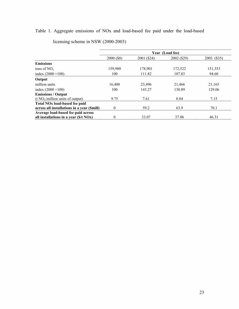
Table 1. Aggregate emissions of NOx and load-based fee paid under the load-based

licensing scheme in NSW (2000-2003)

Year (Load fee) 2000 ($0) 2001 ($24) 2002 ($29) 2003 ($35) Emissions tons of NOx 159,980 178,901 172,522 151,353 index (2000 =100) 100 111.82 107.83 94.60 Output million units 16,400 23,496 21,466 21,165 index (2000 =100) 100 143.27 130.89 129.06 Emissions / Output (t NOx/million units of output) 9.75 7.61 8.04 7.15 Total NOx load-based fee paid across all installations in a year ($mill) 0 59.2 63.9 70.1 Average load-based fee paid across all installations in a year ($/t NOx) 0 33.07 37.06 46.31

23

Table 2. Results from estimation of an econometric model of a natural logarithm of NOx

emissions per unit of output from installations in NSW (2000-2003)

Explanatory Levels of Standard variables class variables Estimate Error DF t Value Pr > |t| Intercept 1.4289 0.8137 224 1.76 0.0805

Rate -0.00374 0.00472 224 -0.79 0.4285 FRT 0 -1.0159 0.2431 224 -4.18 <.0001 FRT 1 0 . . . . CZ 1 0.9346 0.3027 224 3.09 0.0023 CZ 2 0.9138 0.2835 224 3.22 0.0015 CZ 7 0 . . . .

IndID 10 -0.4273 0.8229 224 -0.52 0.6041 IndID 12 0.6818 0.7894 224 0.86 0.3886 IndID 13 -2.264 0.7794 224 -2.9 0.004 IndID 14 -1.1822 0.8987 224 -1.32 0.1897 IndID 17 -4.0589 0.8246 224 -4.92 <.0001 IndID 21 -0.7106 0.8129 224 -0.87 0.3829 IndID 27 -3.371 0.9216 224 -3.66 0.0003 IndID 34 6.2847 0.8104 224 7.75 <.0001 IndID 55 0.2843 0.833 224 0.34 0.7332 IndID 56 -2.934 0.8294 224 -3.54 0.0005 IndID 57 -3.361 0.9418 224 -3.57 0.0004 IndID 58 -1.3968 0.9191 224 -1.52 0.13 IndID 60 -2.5527 0.8925 224 -2.86 0.0046 IndID 66 -3.5772 0.9047 224 -3.95 0.0001 IndID 67 -0.3079 0.8466 224 -0.36 0.7165 IndID 68 -2.1878 0.7776 224 -2.81 0.0053 IndID 74 0 . . . .

Covariance parameter estimates

Residual size 0 1.7147 Residual size 1 0.3670

L.R. test for heteroscedasticity 15.47 at 1 d.f.

24

Table 3. Results from an estimation of an econometric model of the first difference of

NOx emissions per unit of output from installations in NSW (2000-2003)

Explanatory Levels of Standard variables class variables Estimate Error DF t Value Pr > |t| Intercept -0.5554 8 168 -0.07 0.9447

Rate 0.02584 0.1687 168 0.15 0.8785 FRT 0 -0.224 3.9174 168 -0.06 0.9545 FRT 1 0 . . . . CZ 1 -0.02265 3.1113 168 -0.01 0.9942 CZ 2 -0.2004 2.838 168 -0.07 0.9438 CZ 7 0 . . . .

IndID 10 0.08847 7.1893 168 0.01 0.9902 IndID 12 0.01716 134.45 168 0 0.9999 IndID 13 0.03514 5.098 168 0.01 0.9945 IndID 14 0.1008 8.2492 168 0.01 0.9903 IndID 17 0.0215 5.476 168 0 0.9969 IndID 21 0.009317 5.9983 168 0 0.9988 IndID 27 -0.2027 7.1645 168 -0.03 0.9775 IndID 34 17.6988 6.9179 168 2.56 0.0114 IndID 55 -0.1302 190.06 168 0 0.9995 IndID 56 0.09319 5.5571 168 0.02 0.9866 IndID 57 0.07125 7.4081 168 0.01 0.9923 IndID 58 0.3536 6.4313 168 0.05 0.9562 IndID 60 -0.00135 6.3103 168 0 0.9998 IndID 66 0.001583 6.1983 168 0 0.9998 IndID 67 0.05297 134.48 168 0 0.9997 IndID 68 0.008241 5.4667 168 0 0.9988 IndID 74 0 . . . .

Covariance parameter estimates

Residual size 0 71.9674 Residual size 1 110831

L.R. test for heteroscedasticity 623.43 at 1 d.f.

25

Figure 1. Plot of physical output vs. NOx emissions from installations in NSW (2000-

2003)

0

5000

10000

15000

20000

25000

145,000 150,000 155,000 160,000 165,000 170,000 175,000 180,000 185,000

NOx emisions (tons)

Out

put (

mill

ion

units

)

2002 2000 2001

1999

26