1 - 1

Liquefaction Hazard Zonation, case study Bhuj, India.

Cees van Westen (E-mail : westen@itc.nl)* P.K.Champati ray (IIRS) (E-mail: )** *International Institute for Geo-Information Science and Earth Observation, ITC P.O. Box 6, 7500 AA Enschede, The Netherlands **

Disclaimer The material in this exercise is for training purposes only. The results should not be used in actual planning of the city of Bhuj as ITC does not guarantee the accuracy and precision of the input data. The GIS software that will be used in this exercise is the Integrated Land and Water Information System (ILWIS), version 3.11, developed by the International Institute for Geo-Information Science and Earth Observation (ITC). Information: www.itc.nl

1.1 Objective: The objective of this exercise is to assess the liquefaction hazard for the the city of Bhuj using modeling techniques in a GIS, based on the methodology given by HAZUS technical manual of FEMA, USA.

Case study Bhuj: Liquefaction hazard modelling

1 - 2

1.2 Introduction On January 26, 2001, a magnitude 7.7 earthquake devastated this area, killing 20,000 people and destroying buildings, dams, and port facilities. The earthquake epicenter was about 70 kilometers northeast of the city of Bhuj. The earthquake may have occurred on the Kachchh Mainland Fault, which extends from the region of the epicenter westward along the curved boundary between the darker brown region to the south and the lighter brown area north of it. The compressive stresses responsible for the earthquake are related to the collision of India with Asia and the resulting rise of the Himalayas to the northeast. That part of the Kachchh region which lies north of the Kachchh Mainland Fault includes the Banni Plains and the Rann of Kachchh. It is a low, flat basin characterized by salt pans and mud flats. The salt forms in the Rann of Kachchh as mineral-laden waters evaporate. During the earthquake, strong shaking produced liquefaction in the fine silts and sands below the water table in the Rann of Kachchh. This caused the mineral grains to settle and expel their interstitial water to the surface. Field investigations have found abundant evidence of mud volcanos, sand boils, and fissures from which salty ground water erupted over an area exceeding 10,000 square kilometers. The killer earthquake on 26th January, 2001, the 51st Republic Day of India was accompanied by large scale discharge of subsurface (ground) water leading to reports of reemergence of the mythical Saraswati or Indus river. High revisit capabilities of IRS WiFs images have been helpful in studying the persistence of the released water in near real time. Three IRS images prior to the earthquake were analyzed along with a series of post earthquake images of the area to arrive at meaningful conclusion regarding the extent and period of the water surges. WiFs images are also found more useful to study synoptic contiguity of water discharges due to their larger swath as compared to LISS-III images. The water surges are established to be a temporary phenomenon associated with the earthquake. WiFs images of 26 January, 2001 acquired barely 100 minutes after the quake shows emergence of many water sprouts and channels. There is a relative increase in volume of water in the WiFs image of 29th January (compared to 26th January) in some of the places. There after there has been a regular fall in the volume of water, which seem to have completely disappeared on 4th February and 13th February WiFs images. WiFs images of 23rd January, 2001, 20th January, 2001 and 7th January, 1999 were used to assess the pre-quake surface water scenario of the area. Generally, cracks can develop in soil after an earthquake and local ground water may come up along these cracks. This has been clearly demonstrated using IRS WiFs images that all these are completely temporary phenomena.

Fig. 1: WiFs FCC image of 26th January, 2001 depicting the location of sites used for detailed analysis. Site-2 images for a number of dates are shown subsequently. Figure 1 shows the WiFs image of 26th January. The series of WiFs images of a number of dates both before and after the quake (namely 23rd January, 2001, 26th January 2001, 29th January 2001, and 4th January, 2001) for one of the three test sites is shown in Figure-2. All images are two-band false color composite with B4 (near infra red) band assigned to red plane and B3 (red) band being assigned to both green and blue planes of display. The water channels and sprouts appear in dark (black) color, while the dried up water channels appear in cyan as a result of an increase in red (B3) band gray count over near infra red (B4) band. The lower gray count of near infra red band is due to presence of moisture.

Fig. 2a: WiFs image of 23rd January, 2001 before the earth quake Fig. 2b: WiFs image of 26th January, 2001 (First image after the earth quake). Some of water surges are marked using red arrows.

Fig. 2c: WiFs image of 29th January, 2001. This images shows maximum spread of water among all analyzed WiFs images. Red arrows indicate water channels. Fig. 2d: WiFs image of 4th February, 2001 showing already dried up water channels.

Source: http://www.gisdevelopment.net/magazine/gisdev/2001/mar/mws.shtml Other useful websites: Damage report from EERI: http://www.eeri.org/Publications/pub.html SRTM images of Bhuj area: http://www.jpl.nasa.gov/srtm/india_radar_images.html http://earthobservatory.nasa.gov/Newsroom/NewImages/images.php3?img_id=4810

1 - 5

1.3 Evaluating the input data

The input data consists of a series of raster and vector maps.

Input data • Location map: LOCATION –shows prominent places in the study area • Earthquake magnitude: 7.7 • Epicentre: available as a point map: usgsepi • Lithological map: Geology with attribute table Geology • Village Boundary Map: VIL_BND with attribute data on damage • Raster images bhuj misr jan 15 2001 true color and bhuj misr jan 31

2001 true color

In the beginning, kindly see all the data files by displaying and selecting the appropriate column from the respective attribute table.

• Click on the geology vector layer (polygon file), the following screen

appears and select the formation in attribute table, to see the different geological formations. In the representation select litho

• Check the contents of the maps by using the Pixel Information window.

This area is underlain by sedimentary rocks of Mesozoic and Tertiary age and Deccan Traps (basalt). Most importantly this area is predominantly covered by Rann, i.e. salt waste, vast expanse of low lying area covered with salt, which gives almost desert look. Other important feature is the vast tidal flat areas on the south and south eastern margin of the area along the low lying coastal areas.

This vector layer has little bit additional information, beyond the study area, which is clipped in the raster layer, which you can see by clicking on the geology raster layer and then select the appropriate attribute coloumn and representation. Now you can display the location and USGS epicenter point files on the geological map

• Select Layer, Add data layer, Point Map LOCATIONS • Select attribute Name and make sure the option Text is selected • Scroll around and check the geology around the study area.

Case study Bhuj: Liquefaction hazard modelling

1 - 6

1.4 Calculation of PGA

Peak Ground Acceleration is calculated based on the distance from the epicenter, magnitude and attenuation law. In this exercise we will use the following attenuation formula originally given by by Joyner and Boore (1981) and modified as:

Log PGA = 0.249*M- Log(SqrtD)-0.00255*(SqrtD)-0.8 Eq 1

In the first place, the buffer distance from the epicenter is calculated.

Remember, all the relevant GIS and image processing operations appear on right clicking the required data file

• First rasterise the epicenter point map with georeference Bhuj • Using the rasterise point map as source map, calculate the distance

map by selecting distance option in raster operation menu. Give epibuf as the out put file name.

• Now display the epibuf map and click around to check the distance (in meters) values from the epicenter

Finally, the PGA is calculated using the equation 1.

• Enter the following expression in the command line

PGA= 10^(0.249 * 7.7-log(sqrt(epibuf/1000))-0.00255*(sqrt(epibuf/1000)) -0.8)

• Display the PGA map and look around the PGA value, which is

calculated as per the attenuation law

Now the soil and geological information will be incorporated as amplification factor, to estimate their influence on the PGA value.

• Now open the geology attribute table and see the ampli column,

compare the values with the major geology, you will find the following (see table 1):

1 - 7

Table 1. Soil amplification factor

Major rock type

Soil type

Soil amplification factor

Quaternary Soft soil 1.4 Tertiary Rock 1 Deccan Traps Hard rock 0.8 Mesozoics Hard rock (except for soft sandstone bearing

formations like Bhuj, Khadir, Wagad and Kaladonger Formation, which are given value 1)

0.8

Mud Flat Saturated soil 1.5 Rann Soft soil 1.4

• From the attribute table, the amplification map is created by entering the following formula in the command line

Ampli=geology.geology.ampli

• Display the ampli map and check the amplification values • We can calculate now the final PGA by multiplying this ampli map

with the PGA map. We use the following formula. PGAF= PGA * Ampli

• While displaying the PGAF map, you might have noticed that some of the values are larger than 1 near the epicenter. In order to take maximum PGA value as 1, clip all values >1 as 1. Use the following formula in the command line.

PGAFF=iff(PGAF >1,1, PGAF)

PGAFF is the final PGA map with soil amplification as given by the geology and soil conditions of the region.

1.5 Estimation of the liquefaction probability

Liquefaction probability is calculated based on the liquefaction susceptibility and PGA values

P LiquefactionP Liquefaction PGA a

K KP

M wmlSC

SC==

⋅⋅ Equation (2)

P Liquefaction PGA aSC = is the conditional liquefaction probability for a given susceptibility category at a specified level of peak ground acceleration (Table) KM = is the moment magnitude (M) correction factor Kw = is the ground water correction factor Pml = proportion of map unit susceptible to liquefaction (Table 3)

Case study Bhuj: Liquefaction hazard modelling

1 - 8

Correction Factor for Equation (1):

K m = − − +0 0027 00267 0 2055 2 91883 2. . . .M M M M represents the magnitude of the seismic event = 7.7 in this case So Kw = 0.986046 K 0.022dw w= + 0 93. dw represents the depth to the groundwater in feet Relationships between liquefaction probability and peak horizontal ground acceleration (PGA) are defined for the given susceptibility categories in Table 2. These relationships have been defined based on the state-of-practice empirical procedures, as well as the statistical modeling of the empirical liquefaction catalog presented by Liao, et. al. (1988) for representative penetration resistance characteristics of soils within each susceptibility category. Table 2. Relationship between liquefaction probability and peak ground acceleration (Liao et al. 1988)

Table 3. Proportion of map unit that will liquefy in the event of earthquake

Soil type Liquefaction Susceptibility Liq_sc

Proportion of map unit pml

Saturated soil Very high 0.25 Soft soil High 0.2 Rock Moderate 0.1 Hard rock Very low 0.02

Before calculating the Liquefaction probability, first the desired input components are calculated. As the conditional probability is calculated as per the susceptibility category, a susceptibility class map is prepared from the geology attribute table.

• check the geology attribute table. The columns liq_sc and pml indicate the values as shown in Table 3

• Use the values stored in these columns to create attribute maps. Use the following expression

pml=geology.geology.pml liq_sc=geology.geology.liq_sc

• Open the attribute maps and check the values • To calculate the liquefaction conditional probability, we use the

values given in Table 2. The calculation is implemented in ILWIS

Susceptibility Category [ ]P Liquefaction PGA a=

Very High 0 ≤ 9.09 a - 0.82 ≤ 1.0High 0 ≤ 7.67a - 0.92 ≤ 1.0

Moderate 0 ≤ 6.67a -1.0 ≤ 1.0Low 0 ≤ 5.57a -1.18 ≤ 1.0

Very Low 0 ≤ 4.16a - 1.08 ≤ 1.0None 0.0

Case study Bhuj: Liquefaction hazard modelling

1 - 9

as given below in command line. The liq_sc values in the formula indicates respective codes for different classes in domain liq_sc, which may be checked before proceeding.

Liq_pcf= iff (liq_sc=”1”, 9.09 * pgaff – 0.82, iff(liq_sc=”2”, 7.67 *

pgaff – 0.92, iff (liq_sc= “3”, iff(liq_sc=”3”, 6.67 * pgaff –1.0, 4.16* pgaff-1.08))))

PGAFF=iff(PGAF >1,1, PGAF)

• Display the map and check the liquefaction conditional probability values

Now once again check the geology attribute table for ground water table information given in column dw. As the actual well data was not available, approximate values are given as:

Table 4. Representative ground water table

Geological region Groundwater table depth in

feet (dw) Mesozoics, Deccan Traps & Tertiaries, mostly comprising high ground

200

Rann 10 Mud flat 1 Recent deposits (alluvium) 50

• From the dw column values, a new column kw is calculated as:

Kw = 0.022*dw +0.93

• Now an attribute map is created for column kw Kw=geology.geology.kw

• Display the map kw for seeing the distribution of the values

Now all the required inputs for the Liquefaction probability estimation are available in map form, hence we can proceed with its calculation

• Type the following formula in the command line

Liq_prob = (liq_pcf*pml)/(0.986*kw)

• The result can be classified as a Liquefaction Probability Class map using density slicing

• Display the map and check the liquefaction probability in the region, you will observe that in the mudflat Rann region values are high indicating higher probability, which was observed in reality too.

• This can be cross checked by displaying the pre and post satellite images of IRS-IC/ID-LISS-III data and by carefully observing the liquid venting in places like Rann and Kandla mudflat region

Case study Bhuj: Liquefaction hazard modelling

1 - 10

1.6 Lateral spreading The expected permanent ground displacements due to lateral spreading can be determined using the following relationship:

[ ] ( )[ ]E PGD K E PGD PGA PLSC SC a = ⋅ =∆ / Equation (3)

( )[ ]E PGD PGA PL/ SC a = is the expected permanent ground displacement for a given

susceptibility category under a specified level of normalized ground shaking (PGA/PGA(t)) (Figure 1, Table 5)

PGA(t) is the threshold ground acceleration necessary to induce liquefaction (Table 5)

K∆ is the displacement correction factor This relationship for lateral spreading was developed by combining the Liquefaction Severity Index (LSI) relationship presented by Youd and Perkins (1987) with the ground motion attenuation relationship developed by Sadigh, et. al. (1986) as presented in Joyner and Boore (1988) and modified for this study area (equation 1). The ground shaking level has been normalized by the threshold peak ground acceleration PGA(t) corresponding to zero probability of liquefaction for each susceptibility category (Table 5). Figure 1. Expected ground displacement for a given susceptibility category under a specified level of normalize ground shaking (PGA/PGA (t))

0

20

40

60

80

100

0 1 2 3 4 5

PGA/PGA(t)

Disp

lace

men

t (in

ches

) 12x - 12 for 1< PGA/PGA(t)< 2

18x - 24 for 2< PGA/PGA(t)< 370x - 180 for 3< PGA/PGA(t)< 4

Table 5. Threshold Ground Acceleration (PGA(t)) Corresponding to Zero Probability of Liquefaction

Susceptibility Category PGA(t) Very High 0.09g

High 0.12g Moderate 0.15g

Low 0.21g Very Low 0.26g

None N/A

Case study Bhuj: Liquefaction hazard modelling

1 - 11

Correction Factor for equation (3):

K∆ is the displacement correction factor

K . . . .∆ = − + −0 0086 0 0914 0 4698 0 9835M M M3 2 M is moment magnitude = 7.7 in this case, K∆ = 1.141

• check the geology attribute table, column PGAt, which shows the

values as per Table 5: • Now create the attribute map, pgat

Pgat=geology.geology.pgat

• Calculate ratio, of PGA and PGA(t) as: Pgapgat=pgaff/pgat • Now ground displacement (in inch) is calculated as gdisp=iff(pgapgat<1,0,iff(pgapgat<2,12*pgapgat-12,iff(pgapgat<3,18*pgapgat-24,iff(pgapgat<4, 70*pgapgat-180,100)))) • with correction factor, it becomes gdispf= 1.141 * gdisp • Display the map, which can be classified using slicing. The result is a

Ground Displacement Class Map

1.7 Intensity map calculation

Intensity can be calculated from PGA using Trifunac and Brady (1975) Modified Mercalli Intensity Scale (MMI) :

MMI = (Log(PGA * 980) – 0.014) / 0.3

• Calculate the MMI, type the following formula in the command line:

MMI= (log(pgaff*980)-0.014)/0.3

• Display the map and check the intensity values around the study area

Case study Bhuj: Liquefaction hazard modelling

1 - 12

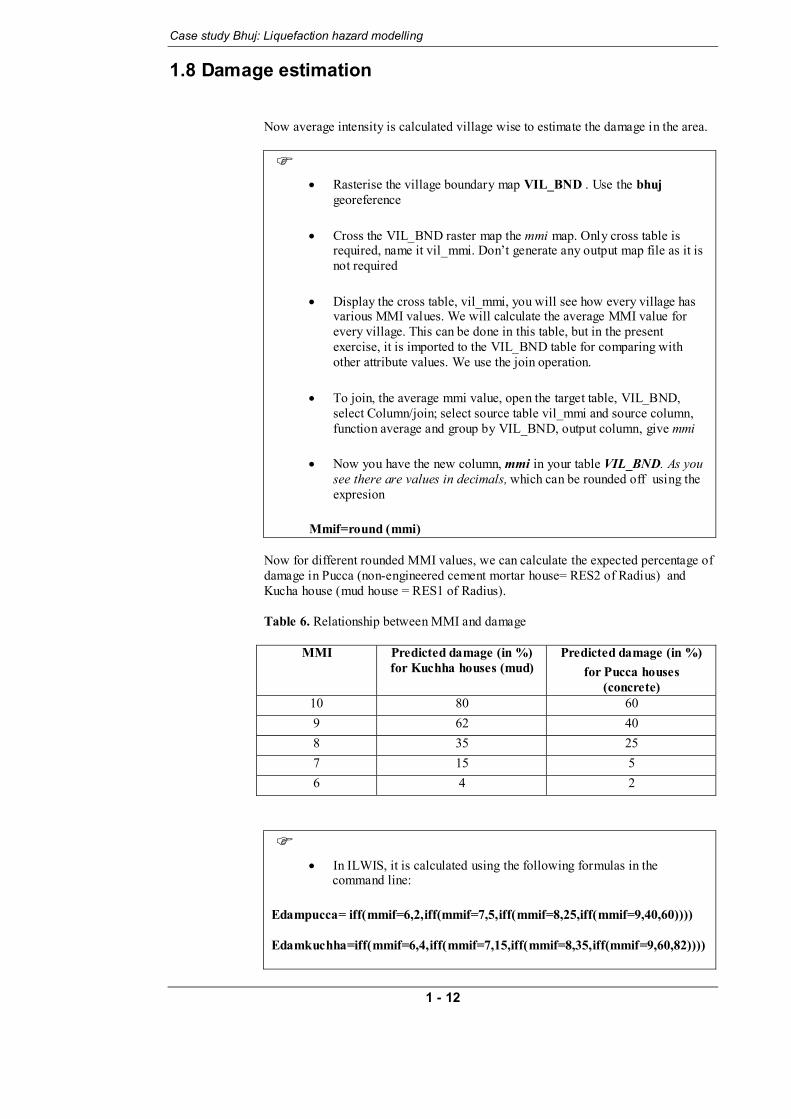
1.8 Damage estimation

Now average intensity is calculated village wise to estimate the damage in the area.

• Rasterise the village boundary map VIL_BND . Use the bhuj

georeference

• Cross the VIL_BND raster map the mmi map. Only cross table is required, name it vil_mmi. Don’t generate any output map file as it is not required

• Display the cross table, vil_mmi, you will see how every village has

various MMI values. We will calculate the average MMI value for every village. This can be done in this table, but in the present exercise, it is imported to the VIL_BND table for comparing with other attribute values. We use the join operation.

• To join, the average mmi value, open the target table, VIL_BND,

select Column/join; select source table vil_mmi and source column, function average and group by VIL_BND, output column, give mmi

• Now you have the new column, mmi in your table VIL_BND. As you

see there are values in decimals, which can be rounded off using the expresion

Mmif=round (mmi)

Now for different rounded MMI values, we can calculate the expected percentage of damage in Pucca (non-engineered cement mortar house= RES2 of Radius) and Kucha house (mud house = RES1 of Radius).

Table 6. Relationship between MMI and damage

MMI Predicted damage (in %)

for Kuchha houses (mud) Predicted damage (in %)

for Pucca houses (concrete)

10 80 60 9 62 40 8 35 25 7 15 5 6 4 2

• In ILWIS, it is calculated using the following formulas in the

command line: Edampucca= iff(mmif=6,2,iff(mmif=7,5,iff(mmif=8,25,iff(mmif=9,40,60)))) Edamkuchha=iff(mmif=6,4,iff(mmif=7,15,iff(mmif=8,35,iff(mmif=9,60,82))))

Case study Bhuj: Liquefaction hazard modelling

1 - 13

The columns P_c, Kutcha_h in table VIL_BND indicate respectively the percentage of actually damaged pucca houses and kuchha houses as found in a survey made by Gujarat govt. The value 101 in those columns indicates no data. The actual and predicted values can be compared. Results may look disappointing, don’t worry, the actual data is not reliable as we have observed in the field. Our observation reveals that the actual damage is in the pattern of predicted, but mostly of higher order.

Now an attribute map can be generated to see the MMI distribution in villages using the expresion: Vil_mmi=vil_bnd.vil_bnd.mmiF This exercise can be done for any earthquake within minutes of knowing the epicenter and magnitude, provided you have a geological map, soil map, water depth and village boundary map ready in digital form. This can also be done for areas prior to earthquake for hypothetical epicenter and magnitude.