Linear system equation

Solve the following system of linear equations:

2 x + y – 4 z = 5x - 2 y - 5 z = - 6.5

y + 2 z = 4

One possible solution is by computing the inverse of the matrix of coefficients:

To do this exercise follow these steps:

Solving linear equations

• Solve the following system of linear equations:• • 2 x + y – 4 z = 5• x - 2 y - 5 z = - 6.5• y + 2 z = 4• • One possible solution is by computing the inverse

of the matrix coefficients: • To do this exercise follow these steps:

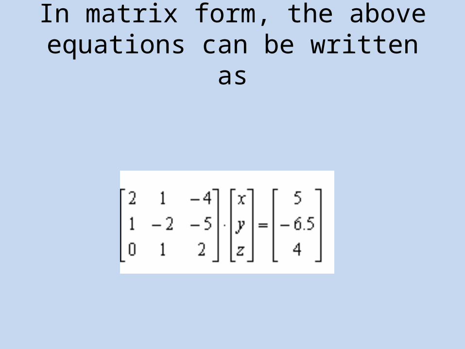
In matrix form, the above equations can be written as

Define the matrix D and the vector M shown below using the same method used in step 1:

Solving linear equations_1% y+4z+x = 10% -2z+3x+4y = 0% -2*z+3*x+4*y = 0'• In general, you can use sym or syms to create

symbolic variables• M_File for solving equations is: clear, syms x y z; eq1 = '2*x-3*y+4*z = 5' eq2 = 'y+4*z+x = 10', eq3 = '-2*z+3*x+4*y = 0' [x,y,z] = solve(eq1,eq2,eq3,x,y,z)

Solving linear equations_2

• % 2 x + y – 4 z = 5• % x - 2 y - 5 z = - 6.5• % y + 2 z = 4• % Multiply the inverse of the matrix D by the

vector M by typing

D=[2 1 4;1 -2 -5;0 1 2]M=[5; -6.5; 4]X=inv(D)*M

Differentiation

• diff_f =df/dx• f = e-axx3bsin(cx)• a, b and c are unspecified constantsclear, syms a b c x; f=exp(-a*x)*x^(3*b)*sin(c*x), diff_f = diff(f,x)

Differentiationf = exp(-a*x)*x^(3*b)*sin(c*x) diff_f = -a*exp(-a*x)*x^(3*b)*sin(c*x)+3*exp(-a*x)*x^(3*b)*b/

x*sin(c*x)+exp(-a*x)*x^(3*b)*cos(c*x)*c

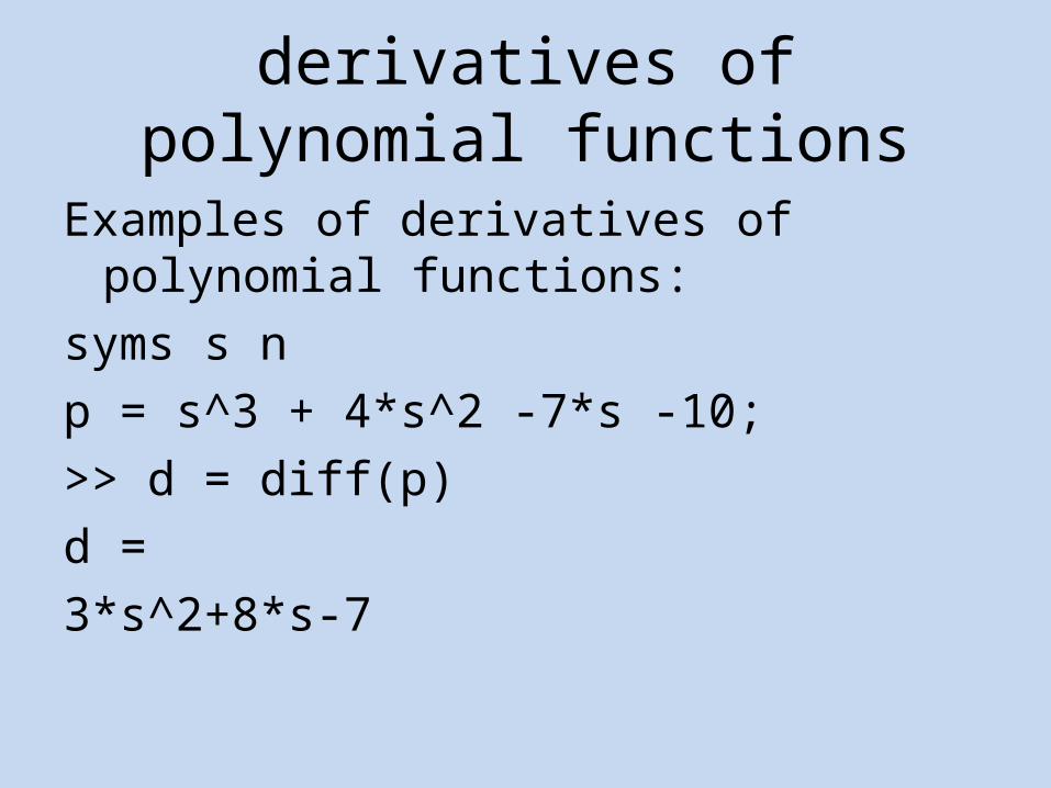
derivatives of polynomial functions

Examples of derivatives of polynomial functions:syms s np = s^3 + 4*s^2 -7*s -10;>> d = diff(p)d =3*s^2+8*s-7

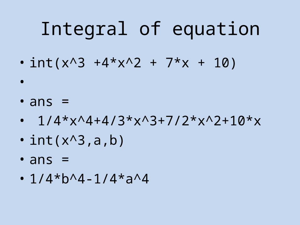
Integral of equation

• int(x^3 +4*x^2 + 7*x + 10)• • ans =• 1/4*x^4+4/3*x^3+7/2*x^2+10*x• int(x^3,a,b)• ans =• 1/4*b^4-1/4*a^4

Integral int(1/x)ans =log(x)>> int(cos(x))ans =sin(x)>> int(1/(1+x^2))ans =atan(x)>> int(exp(-x^2))ans =1/2*pi^(1/2)*erf(x)

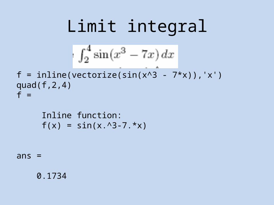
Limit integral

f = inline(vectorize(sin(x^3 - 7*x)),'x')quad(f,2,4)f =

Inline function: f(x) = sin(x.^3-7.*x)

ans =

0.1734

A sample evaluation of a double integral

Infinite integral

We type in:>> f = inline(vectorize((1-u)*sin(u*v*(1-

u))),’u’,’v’)>> dblquad(f,0,1,0,1)

Control Systems Closed-Loop Poles

The closed-loop transfer function is:

thus the poles of the closed loop system are values of s such that 1 + K H(s) = 0

Closed-Loop system• If we write H(s) = b(s)/a(s),• then this equation has the form:

a(s)+kb(s)=0• A(s)/k +b(s)=0• Let n = order of a(s)• and m = order of b(s) • [the order of a polynomial is the highest power of s that appears in it].• We will consider all positive values of k.• In the limit as k -> 0, the poles of the closed-loop system are a(s) = 0 or

the poles of H(s). I• n the limit as k -> infinity, the poles of the closed-loop system are b(s) = 0

or the zeros of H(s).

Plotting the root locus of a transfer function

Consider an open loop system which has a transfer function of

Closed loop systems

• num=[1 7];• den=conv(conv([1 0],[1 5]),conv([1 15],[1

20]));• rlocus(num,den)• axis([-22 3 -15 15])

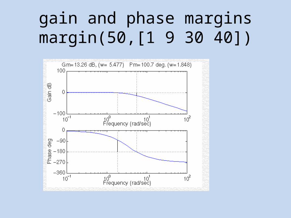
gain and phase margins margin(50,[1 9 30 40])

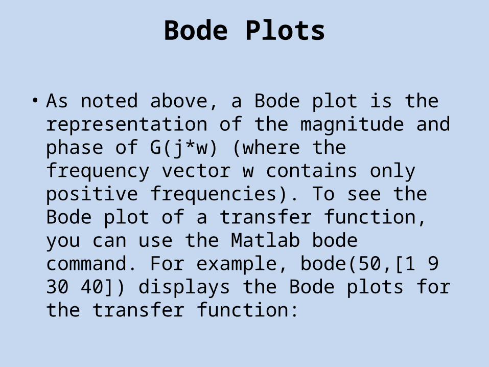
Bode Plots

• As noted above, a Bode plot is the representation of the magnitude and phase of G(j*w) (where the frequency vector w contains only positive frequencies). To see the Bode plot of a transfer function, you can use the Matlab bode command. For example, bode(50,[1 9 30 40]) displays the Bode plots for the transfer function:

bode(50,[1 9 30 40])

bode(1, [1 1])

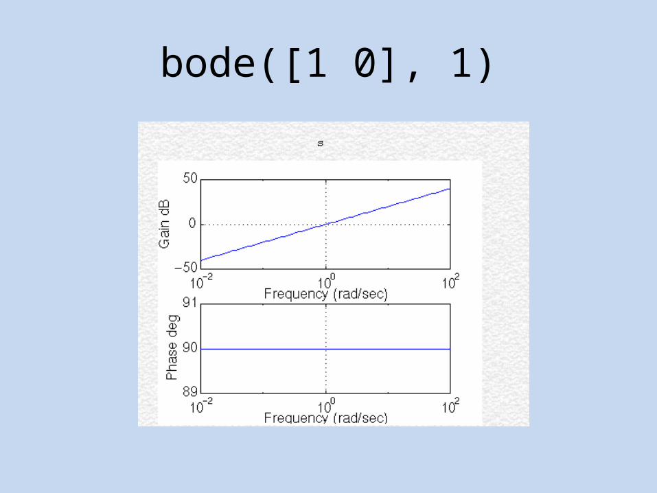
bode([1 0], 1)

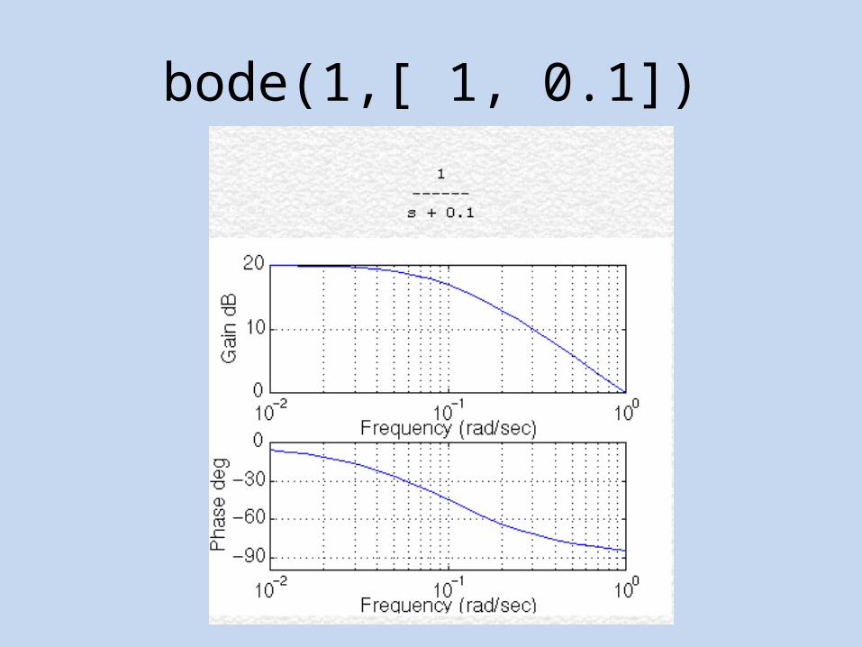
bode(1,[ 1, 0.1])

bode(1,[ 1, 10])

Plot all these bodes

• bode([1, 0.1],1) # S+0.1

• bode([1, 10],1) # S+10

• bode([1 1], 1) # S+1