linear stochastic dynamics lecture 5 outline of lecture 5 · linear stochastic dynamics lecture 5...

Linear Stochastic Dynamics

Lecture 5

1

Outline of Lecture 5

� Stochastic Dynamics of SDOF Systems (cont.).

� Weakly Stationary Response Processes.

� Equivalent White Noise Approximations.

� Gaussian Response Processes as Conditional Normal Distributions.

� Stochastic Dynamics of MDOF Systems.

� Introduction to MDOF Systems.


Lecture 5

2

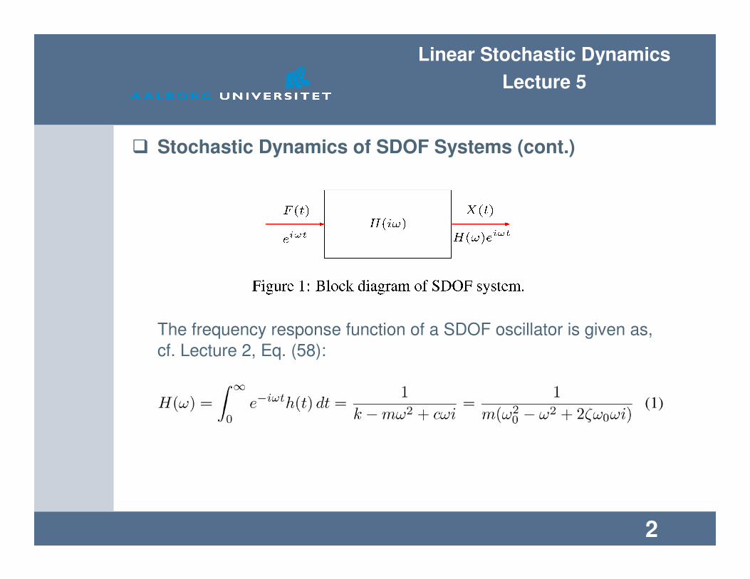
� Stochastic Dynamics of SDOF Systems (cont.)

The frequency response function of a SDOF oscillator is given as,

cf. Lecture 2, Eq. (58):


Lecture 5

3

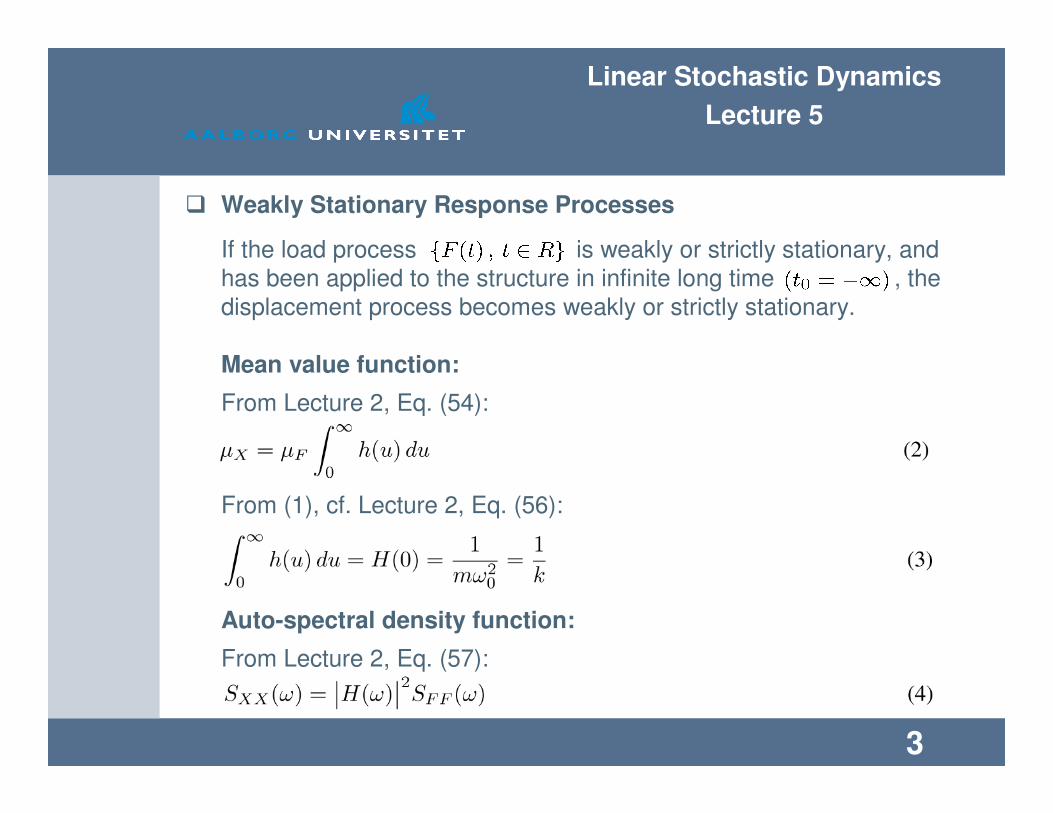
� Weakly Stationary Response Processes

If the load process is weakly or strictly stationary, and

has been applied to the structure in infinite long time , the

displacement process becomes weakly or strictly stationary.

Mean value function:

From Lecture 2, Eq. (54):

From (1), cf. Lecture 2, Eq. (56):

Auto-spectral density function:

From Lecture 2, Eq. (57):


Lecture 5

4

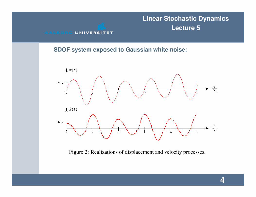
SDOF system exposed to Gaussian white noise:


Lecture 5

5

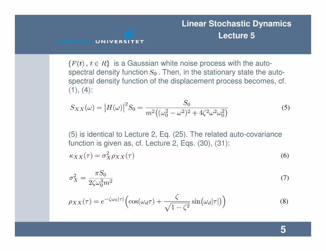
is a Gaussian white noise process with the auto-

spectral density function . Then, in the stationary state the auto-

spectral density function of the displacement process becomes, cf.

(1), (4):

(5) is identical to Lecture 2, Eq. (25). The related auto-covariance

function is given as, cf. Lecture 2, Eqs. (30), (31):


Lecture 5

6

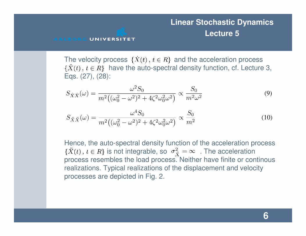
The velocity process and the acceleration process

have the auto-spectral density function, cf. Lecture 3,

Eqs. (27), (28):

Hence, the auto-spectral density function of the acceleration process

is not integrable, so . The acceleration

process resembles the load process. Neither have finite or continous

realizations. Typical realizations of the displacement and velocity

processes are depicted in Fig. 2.


Lecture 5

7

SDOF system exposed to filtered Gaussian white noise:

The load process is obtained by a filtration of a

Gaussian unit intensity white noise process defined

by the auto-covariance and auto-spectral density functions:


Lecture 5

8

The filter is defined by the rational frequency response function of

the order :

Then, the auto-spectral density function of the load process

becomes:

are determined, so (13) at best fits a

given target load spectrum.


Lecture 5

9

The auto-spectral density function of the displacement process

becomes, cf. (4), (13):

The resulting frequency response function is a rational

function of the order , obtained as a product of the components

and :

where , and:


Lecture 5

10

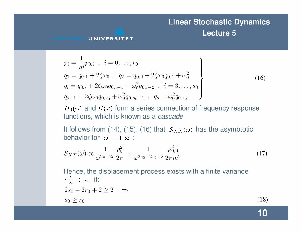
and form a series connection of frequency response

functions, which is known as a cascade.

It follows from (14), (15), (16) that has the asymptotic

behavior for :

Hence, the displacement process exists with a finite variance

, if:


Lecture 5

11

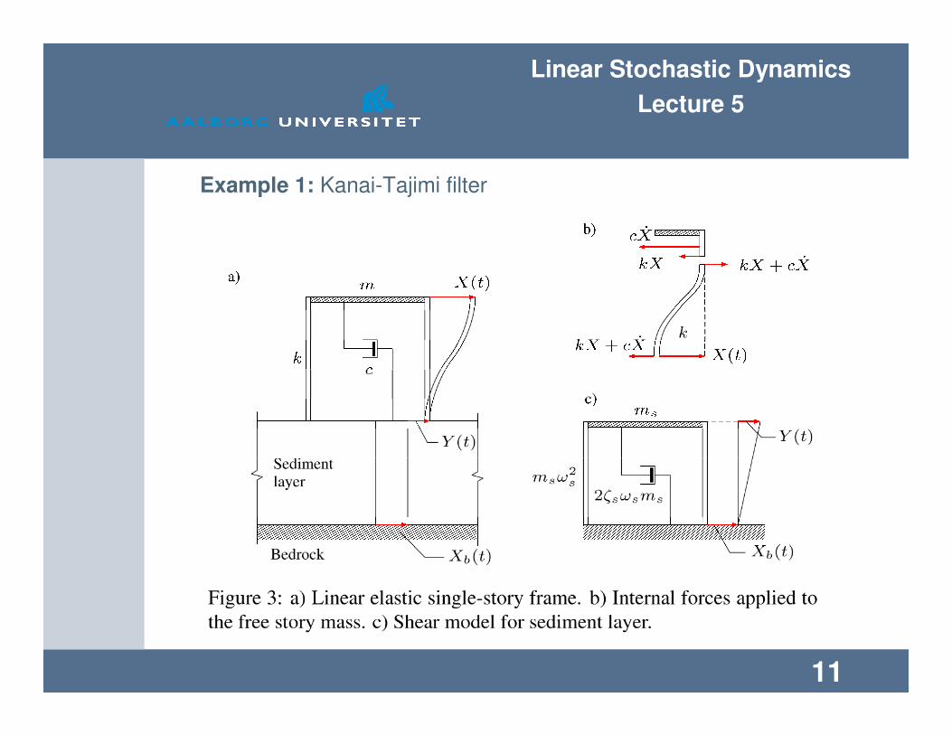
Example 1: Kanai-Tajimi filter


Lecture 5

12

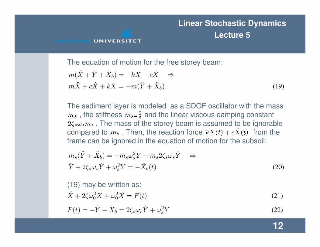
The equation of motion for the free storey beam:

The sediment layer is modeled as a SDOF oscillator with the mass

, the stiffness and the linear viscous damping constant

. The mass of the storey beam is assumed to be ignorable

compared to . Then, the reaction force from the

frame can be ignored in the equation of motion for the subsoil:

(19) may be written as:


Lecture 5

13

where and are the angular eigenfrequency and damping ratio

of the frame:

(20) and (22) determines the earthquake load on the frame as

the output of a rational filter of the order with the filter

constants, cf. (12):

The indicated earthquake model is known as a Kanai-Tajimi filter.

The input to the filter is the bedrock acceleration process

.

The primary energy drain in the subsoil is due to energy transport

carried by the elastic stress waves, and not due to mechanical

dissipation in the soil. For this reason the damping ratio of the

subsoil in the model need to be chosen relatively large, . .


Lecture 5

14

� Example 2: Single-degree-of-freedom system exposed to an

indirectly acting dynamic load and damping force.

� : Point mass at point 1.

� : Damper constant. Damper is acting at point 2.

� : Dynamic load. Load is acting at point 3.

� : Degree of freedom of point mass.

� : Auxiliary degree of freedom of support point of damper.

� : Auxiliary degree of freedom of attack point of load.


Lecture 5

15

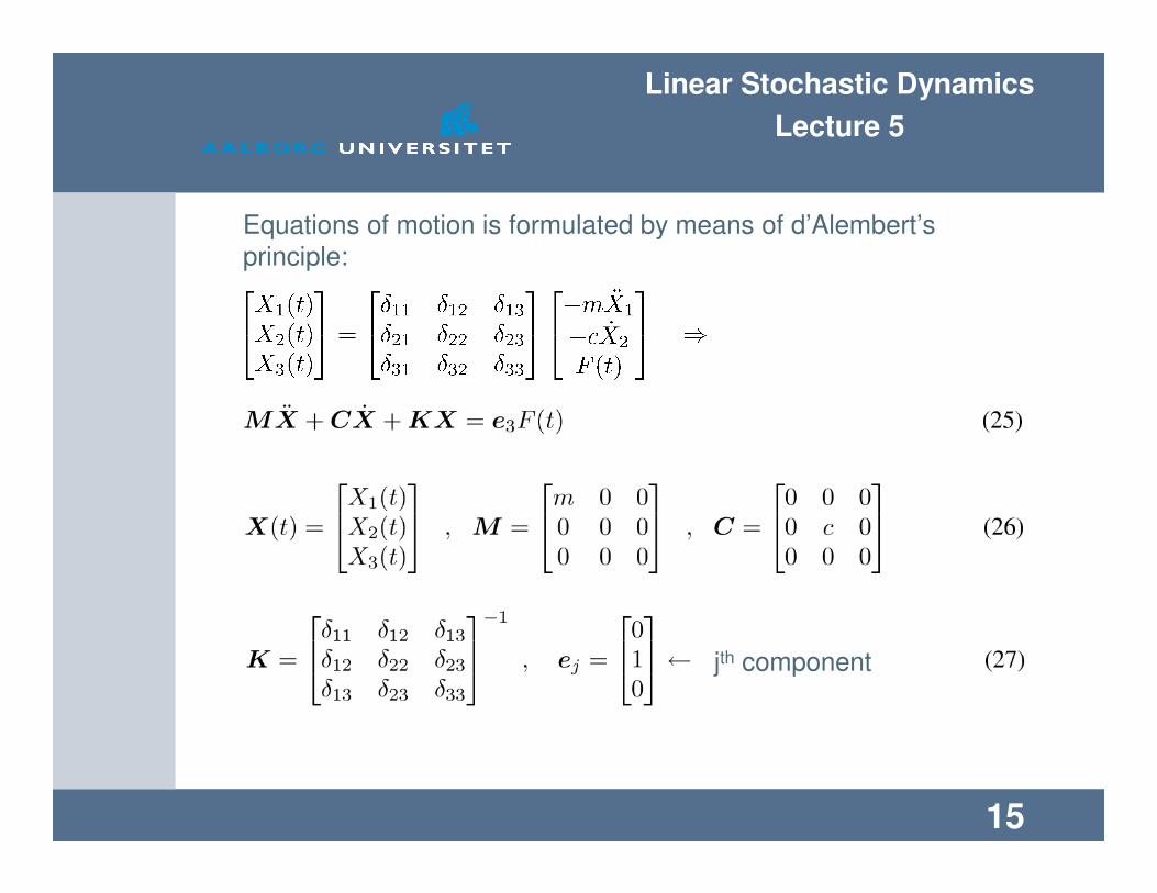
Equations of motion is formulated by means of d’Alembert’s

principle:

jth component


Lecture 5

16

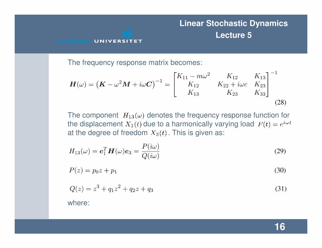
The frequency response matrix becomes:

The component denotes the frequency response function for

the displacement due to a harmonically varying load

at the degree of freedom . This is given as:

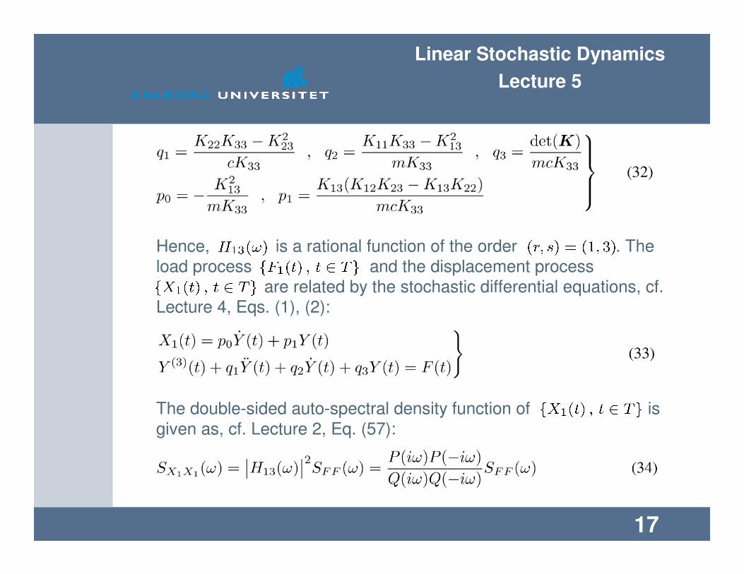
where:


Lecture 5

17

Hence, is a rational function of the order . The

load process and the displacement process

are related by the stochastic differential equations, cf.

Lecture 4, Eqs. (1), (2):

The double-sided auto-spectral density function of is

given as, cf. Lecture 2, Eq. (57):


Lecture 5

18

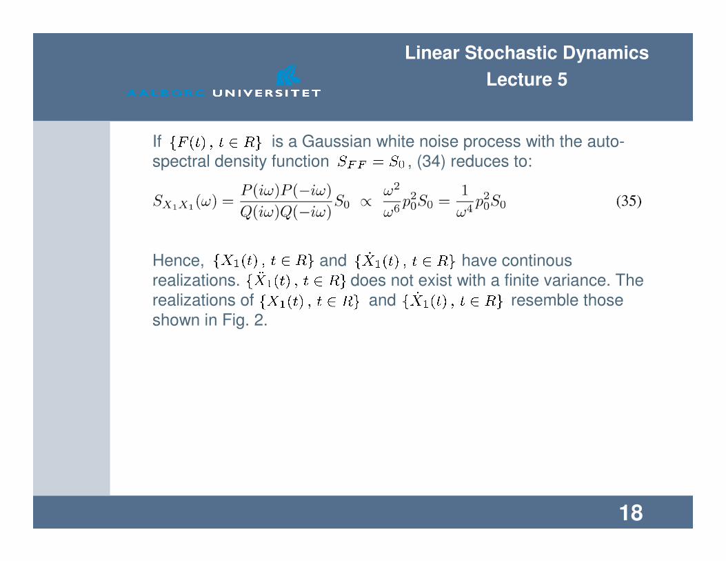
If is a Gaussian white noise process with the auto-

spectral density function , (34) reduces to:

Hence, and have continous

realizations. does not exist with a finite variance. The

realizations of and resemble those

shown in Fig. 2.


Lecture 5

19

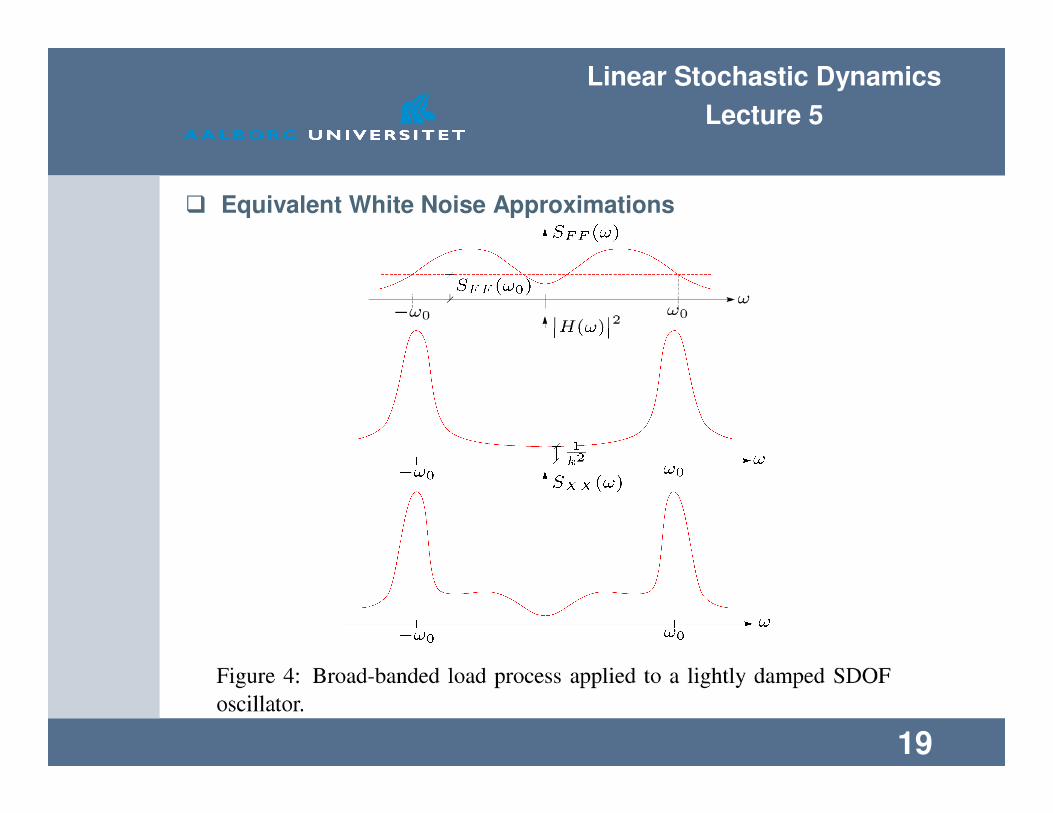
� Equivalent White Noise Approximations


Lecture 5

20

The load process is assumed to be weakly stationary

with a broad-banded auto-spectral density function without

any marked peaks.

The oscillator is assumed to be lightly damped, i.e. . Then,

has a marked peak at . Actually, cf. Eq. (1):

Then, the following approximation for the variance of the

displacement process applies:


Lecture 5

21

Hence, the approximations leading to (37) is equivalent to the

replacement of the actual broad-banded load process with an

equivalent Gaussian white noise process with the auto-spectral

density function , see Fig. 4a. This is so, because only

harmonic load components with angular frequencies close to the

angular eigenfrequency contributes significantly to the variance of

the reponse.


Lecture 5

22


Lecture 5

23

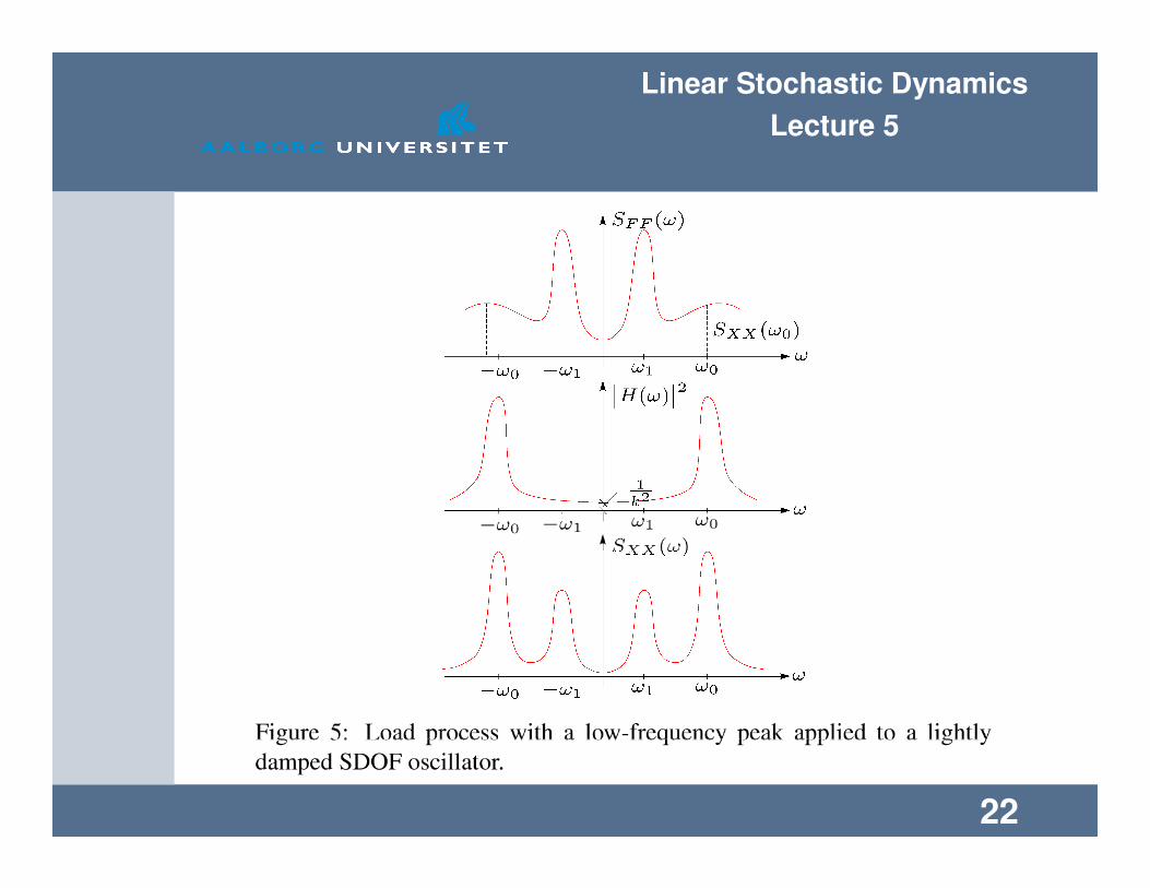
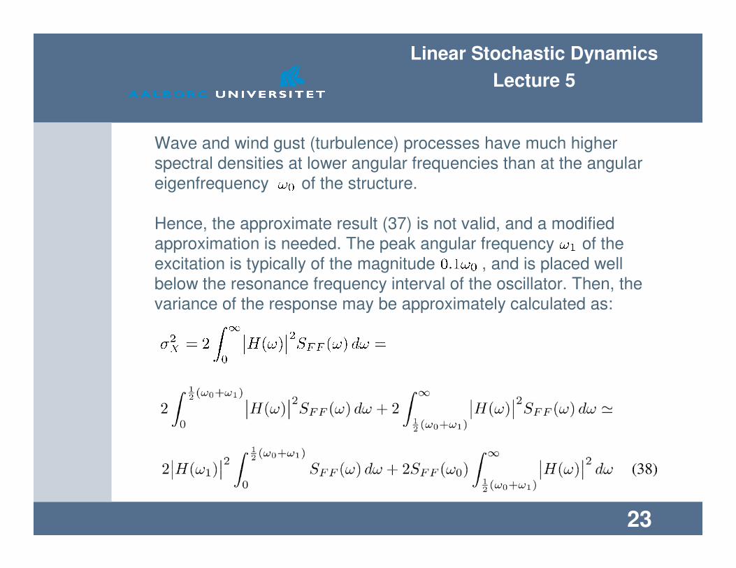
Wave and wind gust (turbulence) processes have much higher

spectral densities at lower angular frequencies than at the angular

eigenfrequency of the structure.

Hence, the approximate result (37) is not valid, and a modified

approximation is needed. The peak angular frequency of the

excitation is typically of the magnitude , and is placed well

below the resonance frequency interval of the oscillator. Then, the

variance of the response may be approximately calculated as:


Lecture 5

24

Next, the following approximations are applied:


Lecture 5

25

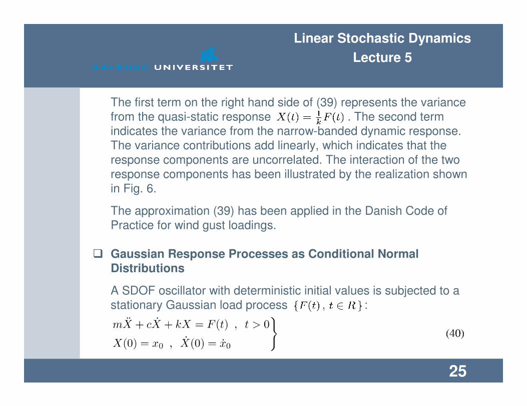
The first term on the right hand side of (39) represents the variance

from the quasi-static response . The second term

indicates the variance from the narrow-banded dynamic response.

The variance contributions add linearly, which indicates that the

response components are uncorrelated. The interaction of the two

response components has been illustrated by the realization shown

in Fig. 6.

The approximation (39) has been applied in the Danish Code of

Practice for wind gust loadings.

� Gaussian Response Processes as Conditional Normal Distributions

A SDOF oscillator with deterministic initial values is subjected to a

stationary Gaussian load process :


Lecture 5

26

Due to the linearity the response process becomes Gaussian as well.

Next, consider the stationary displacement process, obtained as

solution to the stochastic differential equation (40), when the load

process has been acting in infinite long time. The process is defined

by the mean value function and the auto-covariance function

, where is the stationary variance, and

signifies the auto-correlation coefficient function.

The displacement and the velocity at the time are in

this case random variables. Consider the 4-dimensional normal

distributed stochastic vector:

where and denotes the state vector at the times and . The

joint probability density function of becomes, cf. Lecture 1, Eqs.

(20), (21), (22):


Lecture 5

27

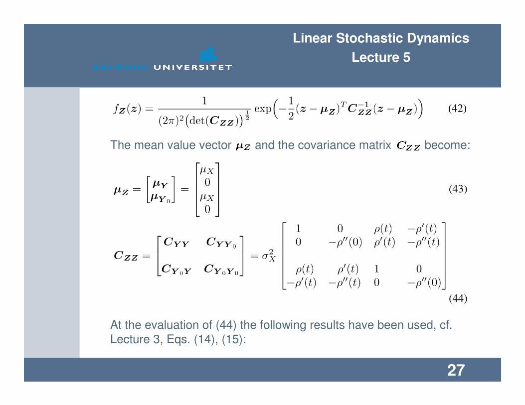
The mean value vector and the covariance matrix become:

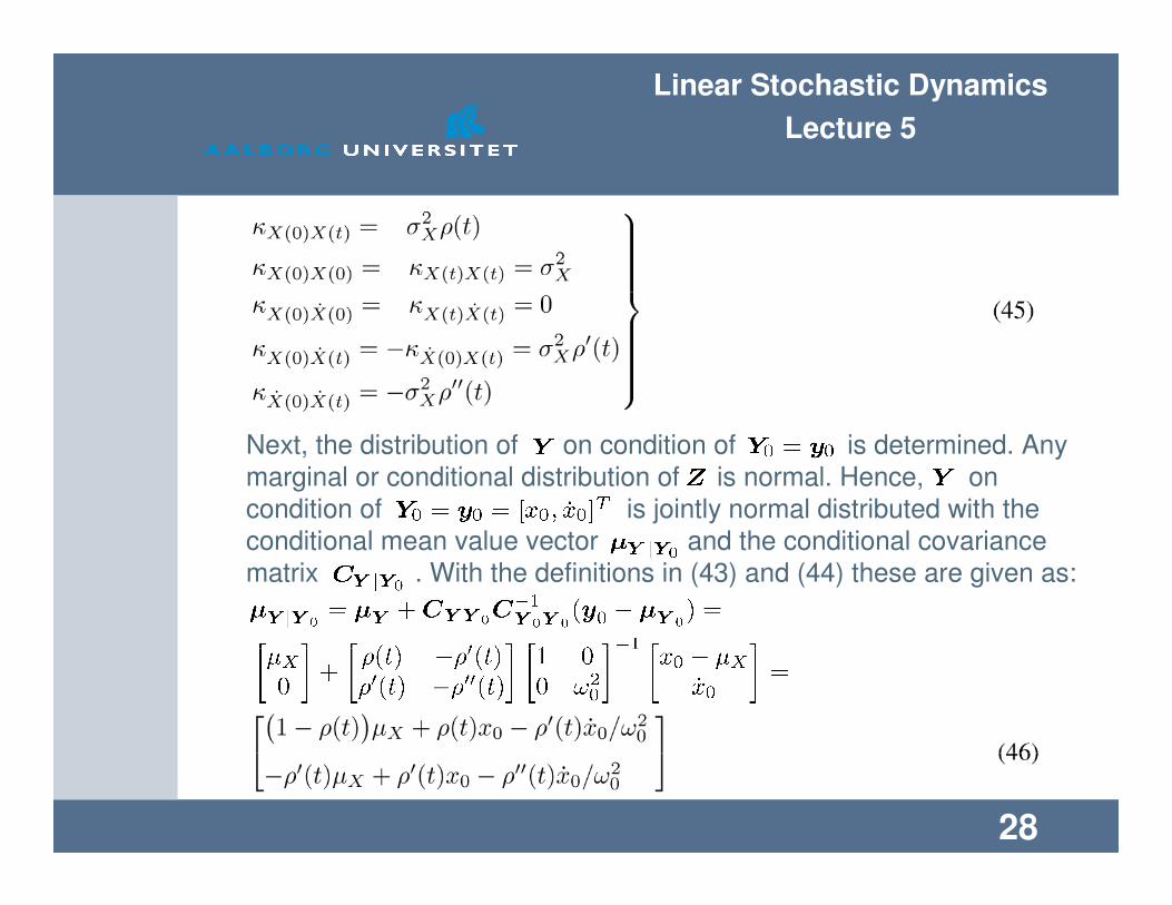
At the evaluation of (44) the following results have been used, cf.

Lecture 3, Eqs. (14), (15):


Lecture 5

28

Next, the distribution of on condition of is determined. Any

marginal or conditional distribution of is normal. Hence, on

condition of is jointly normal distributed with the

conditional mean value vector and the conditional covariance

matrix . With the definitions in (43) and (44) these are given as:


Lecture 5

29

where has been introduced in (46) and (47).

(40) may be formulated on the state vector form, cf. Lecture 4, Eq. (42):


Lecture 5

30

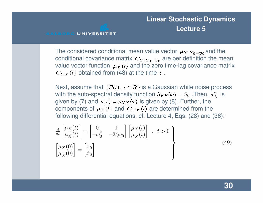
The considered conditional mean value vector and the

conditional covariance matrix are per definition the mean

value vector function and the zero time-lag covariance matrix

obtained from (48) at the time .

Next, assume that is a Gaussian white noise process

with the auto-spectral density function .Then, is

given by (7) and is given by (8). Further, the

components of and are determined from the

following differential equations, cf. Lecture 4, Eqs. (28) and (36):


Lecture 5

31

The differential equations (50) follows by explicit calculation of the

right-hand side of Lecture 4, Eq. (39), cf. Lecture 4, Eq. (44).

From the above argumentation it follows that the solution to (49) and

(50) are given by (46) and (47) for :


Lecture 5

32

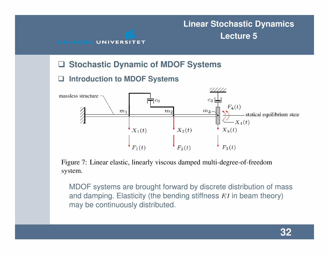
� Stochastic Dynamic of MDOF Systems

� Introduction to MDOF Systems

MDOF systems are brought forward by discrete distribution of mass

and damping. Elasticity (the bending stiffness in beam theory)

may be continuously distributed.


Lecture 5

33

The number of degrees of freedom specifies the number of

unconstrained displacement degrees of each point mass (up to 3

dofs) and the number of unconstrained displacement and rotational

degrees of freedom of each rigid, distributed mass (up to 6 dofs).

� : -dimensional load vector process.

� : -dimensional displacement vector process.

� : Index time interval.

may contain both displacement and rotational

component processes.


Lecture 5

34

Stochastic vector differential equation:

� : Initial value vectors. Stochastic vectors of dimension .

� : Mass matrix .

� : Damping matrix. .

� : Stiffness matrix. .


Lecture 5

35

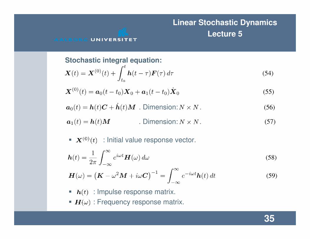
Stochastic integral equation:

� : Initial value response vector.

� : Impulse response matrix.

� : Frequency response matrix.

. Dimension: .

. Dimension: .


Lecture 5

36

Modal analysis:

Undamped eigenvibrations are assumed on the form:

The amplitude vector , the angular frequency and the common

phase are determined by insertion in (53) for , .

This leads to the generalized eigenvalue problem:

Nontrivial solutions for exist for:

Eigensolutions are real, due to the symmetry properties

, , and because or are positive definite.

� : Undamped angular eigenfrequency of the jth mode.

� : Eigenmode.


Lecture 5

37

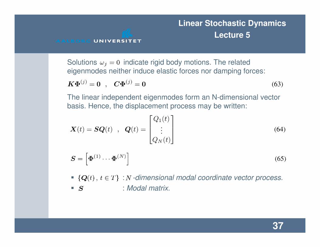
Solutions indicate rigid body motions. The related

eigenmodes neither induce elastic forces nor damping forces:

The linear independent eigenmodes form an N-dimensional vector

basis. Hence, the displacement process may be written:

� : -dimensional modal coordinate vector process.

� : Modal matrix.


Lecture 5

38

Insertion of (64) into (53), and premultiplication with provides:


Lecture 5

39

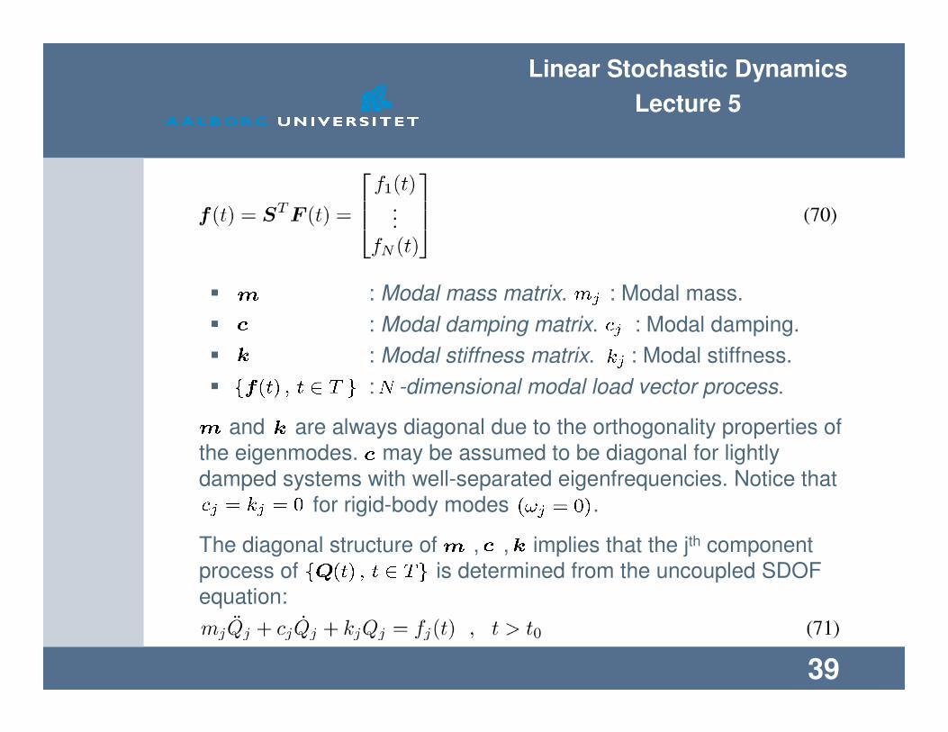
� : Modal mass matrix. : Modal mass.

� : Modal damping matrix. : Modal damping.

� : Modal stiffness matrix. : Modal stiffness.

� : -dimensional modal load vector process.

and are always diagonal due to the orthogonality properties of

the eigenmodes. may be assumed to be diagonal for lightly

damped systems with well-separated eigenfrequencies. Notice that

for rigid-body modes .

The diagonal structure of , , implies that the jth component

process of is determined from the uncoupled SDOF

equation:


Lecture 5

40

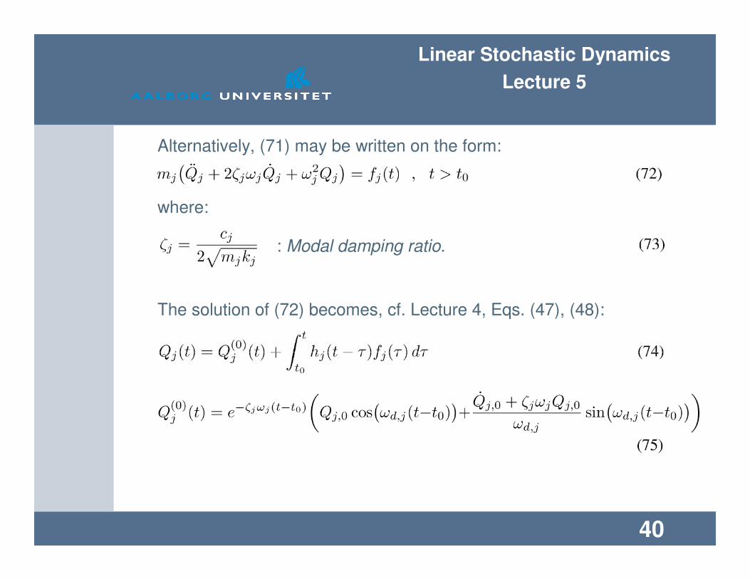
Alternatively, (71) may be written on the form:

where:

The solution of (72) becomes, cf. Lecture 4, Eqs. (47), (48):

: Modal damping ratio.


Lecture 5

41

� : Modal impulse response function of the jth mode.

� : Damped angular eigenfrequency of the jth mode.

� : Frequency response function of the jth mode.


Lecture 5

42

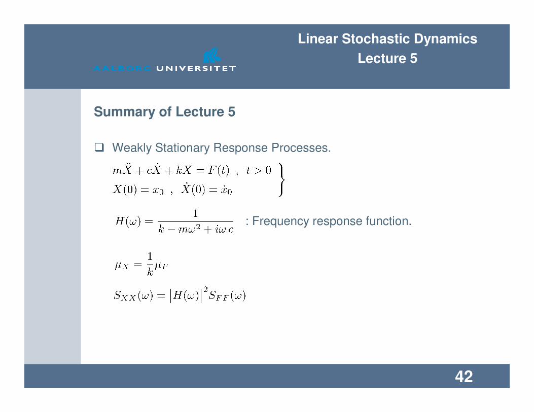
Summary of Lecture 5

� Weakly Stationary Response Processes.

: Frequency response function.


Lecture 5

43

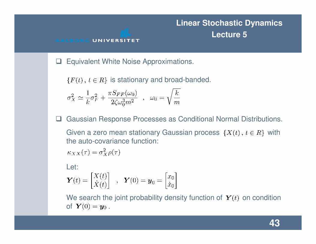
� Equivalent White Noise Approximations.

is stationary and broad-banded.

� Gaussian Response Processes as Conditional Normal Distributions.

Given a zero mean stationary Gaussian process with

the auto-covariance function:

Let:

We search the joint probability density function of on condition

of .


Lecture 5

44

on condition of is normal distributed

, where:

linear stochastic dynamics lecture 5 outline of lecture 5 · linear stochastic dynamics lecture 5...

Documents