learning decision trees with stochastic linear...
TRANSCRIPT

TEL-AVIV UNIVERSITY
RAYMOND AND BEVERLY SACKLER
FACULTY OF EXACT SCIENCES
THE BLAVATNIK SCHOOL OF COMPUTER SCIENCE
Learning Decision Trees with
Stochastic Linear Classifiers
Thesis submitted in partial fulfillment of the requirements
for the M.Sc. degree of Tel-Aviv University
by
Tom Jurgenson
The research work for this thesis has been carried out at
Tel-Aviv University under the supervision of
Prof. Yishay Mansour
June 2017

Acknowledgments
First and foremost, I would like to thank my supervisor, Prof. Yishay Mansour,
who was extremely supportive all throughout this thesis, who was always available
for consultation and provided me with superb guidance and insights.
I would also like to thank my partner Alona and my supportive family (Sum-
mer included) who consistently helped me throughout this process - your support
certainly made it a lot smoother than what it could have otherwise been.

Abstract
We consider learning decision trees in the boosting framework, where we assume
that the classifiers in each internal node come from a hypothesis class HI which
satisfies the weak learning assumption.
In this work we consider the class of stochastic linear classifiers for HI , and
derive efficient algorithms for minimizing the Gini index for this class, although
the problem is non-convex. This implies an efficient decision tree learning algo-
rithm, which also has a theoretical guarantee under the weak stochastic hypothesis
assumption.
1

Contents
1 Introduction 5
2 Related Work 8
3 Model 10
4 Decision Tree Learning Algorithms 12
5 Weak Learning and Stochastic Decision Tree Algorithms 16
6 Stochastic Linear Classifier 18
7 Approximately minimizing the Gini Index efficiently 21
7.1 Algorithms for the linearly independent case: overview . . . . . . 24
7.2 Algorithm FixedPQ - Iterating over pairs of Pw and Qw . . . . . 25
7.3 Algorithm FixedPSearchQ - Iterating over values Pw . . . . . 27
7.4 Algorithm DependentWGI - Dependent case . . . . . . . . . . 27
7.5 Summary . . . . . . . . . . . . . . . . . . . . . . . . . . . . . . 28
8 Empirical Evaluation 29
8.1 Validating Strong Learnability . . . . . . . . . . . . . . . . . . . 29
8.2 Comparison to other classifiers . . . . . . . . . . . . . . . . . . . 33
8.3 Real Data-sets . . . . . . . . . . . . . . . . . . . . . . . . . . . . 35
9 Conclusion 37
2

CONTENTS 3
A Decision tree learning algorithm: pseudo code 40
B Proof of Theorem 5.0.1 43
C Bounding the WGI by regions 46
C.1 Partitioning the WGI to monotone regions . . . . . . . . . . . . . 46
C.2 Overview of the partition to cells . . . . . . . . . . . . . . . . . . 48
C.3 First region: Rb,l . . . . . . . . . . . . . . . . . . . . . . . . . . 49
C.4 Second region: Rb,r . . . . . . . . . . . . . . . . . . . . . . . . . 50
C.5 Third region Ra,l . . . . . . . . . . . . . . . . . . . . . . . . . . 52
C.6 Fourth region Ra,r . . . . . . . . . . . . . . . . . . . . . . . . . 53
C.7 WGI is continuous in p = 0 and p = 1 . . . . . . . . . . . . . . . 54
C.8 Proof conclusion . . . . . . . . . . . . . . . . . . . . . . . . . . 56
C.9 Solution for the dependent case . . . . . . . . . . . . . . . . . . . 56
D Maximizing Information Gain for Pw and Qw 58
D.1 Values of Pw and Qw are given . . . . . . . . . . . . . . . . . . . 59
D.2 Values of Pw and Qw are within specific ranges . . . . . . . . . . 60
D.3 Given value Pw search over Qw . . . . . . . . . . . . . . . . . . 63
D.4 Feasible Ranges for Pw and Qw . . . . . . . . . . . . . . . . . . 66
E Approximation Algorithms 67
E.1 FixedPQ Approximate minimal Gini Index in cells of Pw, Qw . . 68
E.2 FixedPSearchQ Approximate minimal Gini Index in range of Pw 71
E.3 DependentWGI Dependent constraints case . . . . . . . . . . . 74
F WGI not convex 76
G Approximate γ Margin With a Stochastic Tree 78
H Splitting criteria bounds the classification error 81

List of Figures
1.1 Example of decision tree with stochastic linear classifier for learning an
XOR like function. . . . . . . . . . . . . . . . . . . . . . . . . . . 7
7.1 Partition Pw to slices for ρ ≥ 0.5 . . . . . . . . . . . . . . . . . . 25
7.2 Partition (Pw, Qw) to trapezoid cells for ρ ≥ 0.5 . . . . . . . . . 25
8.1 Single Hyperplane Decisions . . . . . . . . . . . . . . . . . . . . 30
8.2 Hyperplane with noise. . . . . . . . . . . . . . . . . . . . . . . . 35
8.3 Multi-dimensional XOR . . . . . . . . . . . . . . . . . . . . . . 35
C.1 The domain R and the sub-domains Ra and Rb (for ρ ≥ 0.5) . . . 48
C.2 WGI: partitioned into regions for ρ ≥ 0.5 . . . . . . . . . . . . . 48
4

Chapter 1
Introduction
Decision trees have been an influential paradigm from the early days of machine
learning. On the one hand, they offer a “humanly understandable” model, and on
the other hand, the ability to achieve high performance using a non-convex model.
Decision trees provide competitive accuracy to other methodologies, such as linear
classifiers or boosting algorithms. In particular, decision forests provide state of
the art performance in many tasks.
Most decision tree algorithms used in practice have a fairly similar structure.
They provide a top-down approach to building the decision tree, where each in-
ternal node is assigned a hypothesis from some hypothesis class HI . The most
notable class is that of decision stumps, namely, a threshold over a single attribute,
e.g., xi ≥ θ. The decision tree algorithm decides which hypothesis to assign in
each internal tree node, to the most part they perform it by minimizing locally
a convex function called splitting criteria. Decision tree algorithms differ in the
splitting criteria they use, for example, the Gini index is used in CART [BFSO84]
and the binary entropy is used in ID3 [Qui86] and C4.5 [Qui93].
From a computational perspective, proper learning of decision tree is hard
[ABF+08]. However, assuming the weak learner hypothesis, as is done in boost-
ing, [KM99] show that decision tree algorithms do indeed boost the accuracy of the
basic hypotheses. Specifically, they show that for a variety of splitting indices, in-
5

Chapter. 1: Introduction 6
cluding Gini index and binary entropy, if one assumes the weak learner assumption,
the resulting decision tree will achieve boosting and guarantee strong-learning.
This work looks at the variation of extending the decision tree algorithms by
allowing a linear classifier at each node. Such decision trees are named oblique
decision trees, originally proposed in CART-LC and developed by [MKS94] and
[HKS93], and extended in a variety of directions [BB98, FAB08, RLSCH12, GMD13,
WRR+16]. However, a clear downside of oblique decision trees is that even mini-
mizing the splitting criteria in an single internal node becomes a non-convex prob-
lem, and the various algorithms resort to methods which converge to a local min-
ima. From a complexity point of view, oblique decision trees with three internal
nodes already encodes three-node neural networks, which is computationally hard
to learn [BR93].
Our Contributions: Our main goal is to perform an efficient computation for se-
lecting a hypothesis in each internal tree node, namely, being able to efficiently
minimize the splitting criteria. We are able to perform this task efficiently for the
related class of stochastic linear classifiers. A stochastic linear classifier has a
weight vector w and given an input x it branches right with probability (x>w +
1)/2, where we assume that x and w are unit vectors. We show how to efficiently
minimize the Gini index for stochastic linear classifiers. We use our efficient Gini
index minimization as part of an overall decision tree learning algorithm. We show,
similar to [KM99], that under the weak stochastic hypothesis assumption our algo-
rithm achieves boosting and strong-learning.
The stochastic linear classifier has a few advantages over other models:
1. Unlike decision trees with decision stumps, it can produce more general de-
cision boundaries which may depend on many attributes.
2. Unlike linear classifiers, it produces a hierarchal structure that allows to fit
non-separable data. (See Figure 1.1 for an illustration of how it fits a non-
separable input.)

Chapter. 1: Introduction 7
2 1 0 1 2
2
1
0
1
2
Predicted
Figure 1.1: Example of decision tree with stochastic linear classifier for learning an XOR
like function.
3. Unlike oblique tree, it can efficiently minimize the splitting criteria for a
single node.
On the downside, since the model becomes more complicated it also becomes less
interpretable than either linear classifiers or decision trees which are based on de-
cision stumps.

Chapter 2
Related Work
Decision tree algorithms are one of the popular methods in machine learning. Most
decision tree learning algorithms have a natural top-down approach. Namely, start
with the entire sample, select a leaf and a hypothesis and replace the leaf by an
internal node that splits using this hypothesis. A main difference between different
decision tree algorithms is in the class of hypotheses HI used and how they select
the splitting hypothesis, e.g., the splitting criteria used.
The two most popular decision trees algorithms are C4.5 by [Qui93] and CART
by [BFSO84]. Both use decision stump as hypotheses in internal nodes. (A deci-
sion stump compares an attribute to a threshold value, e.g., xi ≥ θ.) The differ-
ence between the two algorithms is the specific splitting criteria G(x), where x
is the probability of positive examples within the node. CART uses the Gini in-
dex, i.e., G(x) = 4x(1 − x), while C4.5 uses the binary entropy, i.e., G(x) =
−x log x − (1 − x) log (1− x). One significant benefit of decision stumps is that
the size of the hypothesis class, given a sample of size m, is only dm, where d is
the number if attributes. Since for each attribute we have at most m distinct values
in a sample of size m.
The idea of using linear classifiers for HI , the hypotheses class of the internal
nodes , date back to CART-LC. A clear drawback is that the size of this hypothesis
class is no longer linear in the dimension, but infinite, and minimizing the splitting
8

Chapter. 2: Related Work 9
criteria is potentially a hard computational task. The original proposal of CART-LC
suggested to do a simple gradient decent, which deterministically reaches a local
minima. One of the successful implementation of oblique decision trees is OC1 by
[MKS94], which uses a combination of hill climbing and randomization to search
for a linear classifier of each internal node. Alternative approaches use simulated
annealing by [HKS93] or evolutionary algorithms by [CK03], to generate a linear
classifier in each internal node. The work of [BB98] build a three internal-nodes
decision tree using a non-convex optimization which also maximizes the margins
of the linear classifiers in the three nodes. The work of [WRR+16] uses the eigen-
vector basis to transform the data, and uses decision stumps in the transformed
basis (which are linear classifiers in the original basis).
Even though decision tree algorithm are tremendously popular, due to their effi-
ciency and simplicity, they are challenging to analyze theoretically. [KM99] intro-
duced a framework to analyze popular decision tree algorithms based on the Weak
Hypothesis Assumption of [Sch90]. The Weak Hypothesis Assumption states, that
for any distribution, one can find a hypothesis in the class that achieves better than
random guessing. The main result of their work shows that decision trees can be
used to transform weak learners to strong ones. Qualitatively, assuming the weak
learners always have bias at least γ, decision trees provably achieve an error of
ε with size of (1/ε)O((γε)−2), for the Gini index, and (1/ε)O((γ)−2 log (ε−1)), for
the binary entropy. They also introduce an new splitting criteria which guarantees
a bound (1/ε)O((γ)−2) which is polynomial in 1/ε. We extend the framework of
[KM99] to encompass stochastic linear classifiers, which we use as our hypothesis
class for internal decision tree nodes.

Chapter 3
Model
Let X ⊂ Rd be the domain and Y = {0, 1} be the labels. There is an unknown
distributionD overX×Y and samples are drawn i.i.d. fromD. Given a hypothesis
class H the error of h ∈ H is ε(h) = Pr[h(x) 6= y] where the distribution is both
over the selection of (x, y) ∼ D and any randomization of h.
Given two hypothesis classes HI and HL mapping X to {0, 1} we define
a class of decision tree T (HI , HL) as follows. A decision tree classifier T ∈
T (HI , HL) is tree structure such that each internal node v contains a splitting
function hv ∈ HI and each leaf u contains a labeling function hu ∈ HL. In order
to classify an input x ∈ X using the decision tree T , we start at the root r and
evaluate hr(x). Given that hr(x) = b ∈ {0, 1} we continue recursively with the
subtree rooted at the child node vb. When we reach a leaf l we output hl(x) as the
prediction T (x). In case that HI includes randomized hypotheses we take the ex-
pectation over their outcomes. We denote by ε(T ) the error of the tree, and the set
of leaves in the tree as Leaves(T ). We denote the event that input x ∈ X reaches
node v ∈ T with the predicate Reach(x, v, T ), and when clear from the context
we will use Reach(x, v).
Splitting criterion Intuitively, the splitting criterion G, is a function that mea-
sures how “pure” and large a node is. This function is used to rank various possible
10

Chapter. 3: Model 11
splits of a leaf v using a hypothesis from HI . Formally G is a permissible splitting
criterion: if G : [0, 1]→ [0, 1] and has the following three properties:
1. G is symmetric about 0.5. Thus, ∀x ∈ [0, 1] : G(x) = G(1− x).
2. G is normalized: G(0.5) = 1 and G(0) = G(1) = 0.
3. G is strictly concave.
Three well known such functions are:
1. Gini index: G(q) = 4q(1− q)
2. The binary Entropy: G(q) = −q log (q)− (1− q) log (1− q)
3. sqrt criterion: G(q) = 2√q(1− q).
One can verify that any permissible splitting criteriaG has the property thatG(x) ≥
2 min{x, 1− x} and therefore upper bounds twice the classification error (see ap-
pendix H).

Chapter 4
Decision Tree Learning
Algorithms
The most common decision tree learning algorithms have a top-down approach,
which continuously split leaves in a greedy manner. The algorithms work in iter-
ations, where in each iteration one leaf is split into two leaves using a hypothesis
from HI . The decision which leaf to split and which hypothesis from HI to use to
split it is governed by the splitting criteria G.
Let us start with a few definitions which will help clarify the role of the splitting
criteria G. For simplicity we will describe it using the distribution over examples,
and later we will explain how it works on a sample. Fix a given decision tree T .
We define the probability of reaching node v ∈ T as:
weight(v) = Pr(x,y)∼D
(Reach(x, v))
and its purity as:
purity(v) = Pr(x,y)∼D
(y = 1|Reach(x, l))
which is the probability of a positive label conditioned on reaching node v.
The score of the splitting criterionGwith respect to a decision tree T is defined
12

Chapter. 4: Decision Tree Learning Algorithms 13
as follows,
G(T ) =∑
l∈Leaves(T )
weight(l) ·G(purity(l)). (4.1)
This is essentially the expected value of G(purity(l)) when we sample a leaf
l using the probability distribution D over the tree T . Recall that G is an upper
bound on the error, and therefore G(T ) is an upper bound on the error using T .
This explains the motivation of minimizing G(T ).
The decision tree algorithms iteratively split leaves, with the goal of minimiz-
ing the score of the tree. Let Split(T, l, h) be the operation that splits leaf l using
hypothesis h. The inputs of Split(T, l, h) are: T a tree, l ∈ Leaves(T ) a leaf
and a hypothesis h ∈ HI . The output of Split(T, l, h) is a tree T ′ where leaf l is
replaced by an inner node v which has a hypothesis h and two children v0 and v1,
where v0 and v1 are leaves. When using the resulting tree, and input x that reaches
v then h(x) = b implies that x continues to node vb. Notice that the split is local,
it influences only inputs that reached leaf l in T .
The selection of which leaf and hypothesis to use is based on greedily mini-
mizing G(T ). Consider the change in G(T ) following Split(T, l, h)
∆l,h =G(T )−G(Split(T, l, h)) (4.2)
=weight(l) ·G(purity(l))−∑
b∈{0,1}
(weight(vb) ·G(purity(vb)))
where v0 and v1 are the leaves that result from split leaf l. The algorithm would
need to find for each leaf l the hypothesis h ∈ HI which maximizes ∆l,h. This can
be done by considering explicitly all the hypothesis in HI , in the case where HI
is small, or by calling some optimization oracle. For now, we will abstract away
this issue and assume that there is an oracle that given l returns h ∈ HI which
maximizes ∆l,h, hence minimize G(T ).
We now describe the iterative process of building the decision tree. Initially,
the tree T is comprised of just the root node r. We split node r using the hypothesis

Chapter. 4: Decision Tree Learning Algorithms 14
h which maximizes ∆r,h (thus minimizing G(T )). In iteration t, when we have a
current tree Tt, we consider each leaf l of Tt and compute the hypothesis hl ∈ HI
which maximizes ∆l,h using the oracle. We select the leaf that can guarantee the
largest decrease, i.e., lt = max argl,h ∆l,h, and set Tt+1 = Split(T, lt, hlt).
When the decision algorithm terminates it assigns a hypothesis from HL to
each leaf. Many decision tree learning algorithms simply use a constant hypothesis
which is a label, i.e., {0, 1}. Our framework allows for a more elaborate hypothesis
at each leaf, we only assume that the error of the hypothesis at leaf l is at most
min{x, 1− x} where x = purity(l).
Using a sample: Clearly the decision tree algorithms do not have access to the
true distribution D but only to a sample S. Let S be a sample of examples sampled
from D (S is a multiset) and let DS be the empirical distribution induced by S.
We simply redefine the previous quantities using the empirical distribution DS .
Specifically,
weight(v) = Pr(x,y)∼DS
(Reach(x, v)) =|{(x, y) ∈ S : Reach(x, v) = TRUE}|
|S|
purity(v) =
Pr(x,y)∼DS
(y = 1|Reach(x, l)) =|{(x, y) ∈ S : Reach(x, v) = TRUE, y = 1}||{(x, y) ∈ S : Reach(x, v) = TRUE}|
As a result of this change the expressions for G(T ) and ∆l,h in equations (4.1) and
(4.2) are maintained. This allows the use of the Top-Down approach as specified
without any further modifications.
Stochastic Hypothesis: We would like to extend the setting to allow for stochas-
tic hypothesis. A major difference between the stochastic and deterministic case is
that in the deterministic case the tree partitions the inputs (according to the leaves)
while in the stochastic case we have only a modified distribution over the input
induced by the leaves. This implies that now, given a tree T , each input x is asso-
ciated with a distribution over the leaves of T . This requires modifications to the

Chapter. 4: Decision Tree Learning Algorithms 15
basic decision tree learning algorithm, most notably maintaining the distribution
over the leaves, per input x. The probability of reaching a node v, whose a path in
the tree is 〈(h1, b1)...(hk, bk)〉 where hi ∈ HI and bi ∈ {0, 1}, is
Pr(x,y)∼D
(Reach(x, v)) = Pr (∀i ∈ [1, k] : hi(x) = bi)
=k∏i=1
Pr (hi(x) = bi|hj(x) = bj , j < i)
For this reason the modified decision tree learning algorithm keeps for each
input x a distribution over the current leaves of T (In contrast, in the deterministic
case, each input x has a unique leaf). When evaluating the reduction in the split-
ting criteria G, at a leaf v, we compute the distribution over the sample, which is
associated with the current node v (in contrast, in the deterministic case, each node
v is associated with a subset of the inputs).
A detailed description of the top-down decision tree learning algorithm DTL
for a stochastic hypotheses class is provided in Appendix A.

Chapter 5
Weak Learning and Stochastic
Decision Tree Algorithms
In this section we extend the results about the boosting ability of deterministic
decision trees to include stochastic classifiers in the internal nodes. Since we have
stochastic hypothesis we need that the weak learner assumption would hold for the
expected error. Next, we slightly modify the existing analysis and show that the
same boosting bounds that hold in the deterministic case hold also in the stochastic
case. We start by defining the weak learning assumption.
Assumption 5.0.1 (Weak Stochastic Hypothesis Assumption). Let f be any boolean
function over the input space X . Let H be a class of stochastic boolean functions
over X . Let γ ∈ (0, 0.5]. We say H γ-satisfies the Weak Stochastic Hypothesis
Assumption with respect to f if for every distribution D over X , there exists an
hypothesis h ∈ H such that:
Prx∼D
(f(x) 6= h(x)) ≤ 0.5− γ
where the probability is both over the distribution D, and the randomness of h.
Similar to [KM99], we show the following theorem,
16

Chapter. 5: Weak Learning and Stochastic Decision Tree Algorithms 17
Theorem 5.0.1. Let H be any class of stochastic boolean functions over input
space X . Let γ ∈ (0, 0.5], and let f be any target function such that H γ-satisfies
the Weak Stochastic Hypothesis Assumption with respect to f . LetD be any target
distribution, and let T be the tree generated by DTL(D, f,G, t) with t iterations.
Then for any target error ε, the error ε(T ) is less than ε provided that:
t ≥(
1
ε
)c/(γ2ε2 log (1/ε))
if G(q) = 4q(1− q)
t ≥(
1
ε
)c log (1/ε)/γ2
if G(q) = H(q)
t ≥(
1
ε
)c/γ2if G(q) = 2
√q(1− q)
The above theorem establishes a tradeoff between the desired error ε, the bias
parameter γ of the Weak Stochastic Hypothesis Assumption, the splitting criteria
G and the decision tree size t. The proof is provided in Appendix B.

Chapter 6
Stochastic Linear Classifier
In this section, we describe the stochastic linear classifier which we use for the
hypothesis classHI , which are the hypotheses used in the internal nodes of the tree.
We will also derive some basic properties which will be useful for our derivations.
Let S = {〈xi, yi〉} be a sample of size N drawn from D. Let Dv be a dis-
tribution over S, i.e., Dv(xi) ≥ 0 and∑N
i=1Dv(xi) = 1. (We will have various
distributions over the sample S, when we consider different nodes of the tree.) We
assume that the inputs xi are normalized to norm 1, i.e., ‖xi‖2 = 1. We denote the
weight of the positive examples according to Dv by ρ, i.e., ρ =∑N
i=1 yiDv(xi).
For the Stochastic Linear Classifier we will have a weight vector w, which we
assume is also normalized to norm at most 1, i.e., ‖w‖2 ≤ 1. Our classification
would induce a probability
Pr[y = 1|x,w] =w · x+ 1
2
Note that since ‖w‖ ≤ 1 and ‖x‖ = 1 then |w · x| ≤ 1 and therefore
0 ≤ Pr[y = 1|x,w] ≤ 1.
We like to define two measures that w induces. The first is Pw, the weight of
samples classified as positive by w. Formally,
Pw =N∑i=1
Dv(xi)w · xi + 1
2. (6.1)
18

Chapter. 6: Stochastic Linear Classifier 19
Note that 0 ≤ Pw ≤ 1, since∑N
i=1Dv(xi) = 1 and 0 ≤ w·xi+12 ≤ 1.
We define by Qw the weight of positive labels in the samples classified by w
as positive. Formally,
Qw =
N∑i=1
Dv(xi)w · xi + 1
2yi. (6.2)
Clearly 0 ≤ Qw since all the terms are non-negative. We can upper bound Qw by
Pw, since yi ≤ 1:
Qw =
N∑i=1
Dv(xi)w · xi + 1
2yi ≤
N∑i=1
Dv(xi)w · xi + 1
2· 1 = Pw
and we can bound Qw by ρ since w·xi+12 ≤ 1:
Qw =
N∑i=1
Dv(xi)w · xi + 1
2yi =
N∑i=1|yi=1
Dv(xi)w · xi + 1
2≤
N∑i=1|yi=1
Dv(xi) = ρ
Finally, we can also lower bound Qw by Pw − (1− ρ) since:
Pw −Qw =
N∑i=1
Dv(xi)w · xi + 1
2(1− yi) ≤
N∑i=1
Dv(xi)(1− yi) = 1− ρ
Therefore,
max{0, Pw − 1 + ρ} ≤ Qw ≤ min{Pw, ρ} . (6.3)
Some intuition about the above bounds: since Qw is a subset of positive labeled
samples it is bounded by ρ, and since it is a subset of the samples the classifier
classifies as positive, it is bounded by Pw. Also, clearly it is lower bounded by 0
and also lower bounded by the fraction of positives samples minus the fraction of
the negative predictions of the classifier, i.e., 1− Pw.
We can also write Pw and Qw in vector notation, which sometimes would be
more convenient. For this purpose we denote the distribution Dv ∈ RN as a vector
over the sample inputs, X ∈ RN×d the examples matrix and y ∈ {0, 1}N the
labels of the examples. Using this notation we have:
Pw =1
2D>v Xw +
1
2(6.4)

Chapter. 6: Stochastic Linear Classifier 20
Qw =1
2(Dv � y)>Xw +
ρ
2, (6.5)
where the � signal is element-by-element multiplication.
The values of Pw and Qw play an important role in evaluating candidate clas-
sifiers w by plugging them into the splitting criteria, as explained in more details
in the next section.
Remark. One may wonder what will be the stochastic effect on the linear clas-
sifier behavior. Note that if w is a deterministic linear classifier with margin γ,
then it implies that when we use w as a stochastic linear classifier we “err” with
probability (1 − γ)/2. We can amplify the success probability by having a tree
of depth O(γ−2 log ε−1) and reducing the error probability to ε. For more details
please refer to appendix G.

Chapter 7
Approximately minimizing the
Gini Index efficiently
In the previous section we presented the stochastic linear classifiers, which we will
use to split internal nodes in the tree, i.e., the class HI is the set of all stochastic
linear classifiers with norm at most 1. We would like to use the generic top-down
decision tree learning approach in order to greedily minimize the value of the split-
ting criteria, and thus minimizing indirectly the prediction error.
In this section we will discuss how we select a hypothesis fromHI to minimize
the value splitting criteria. Recall that we like to maximize ∆l,w for a given leaf l
over all stochastic linear classifiers w. Given a leaf l, the distribution Dl over the
samples that reach it, and the probability of the positive examples in Dl is ρ, we
would like to find a w that maximizes the drop in the splitting criteria, namely
arg maxw
∆l,w
= arg maxw
weight(l)
(G(ρ)−
(Pw ·G
(QwPw
)+ (1− Pw)G
(ρ−Qw1− Pw
)))= arg min
w
(Pw ·G
(QwPw
)+ (1− Pw)G
(ρ−Qw1− Pw
))We notice that the splitting criteria value is comprised of two parts: the first,
G(ρ) is the current purity measure and it has the same value for every w, and
21

Chapter. 7: Approximately minimizing the Gini Index efficiently 22
therefore does not influences the optimization (therefore it is dropped in the last
line). The second part, is the purity induced by the split w, which we like to
minimize.
In this work we will focus on the case Gini Index, GI , as the splitting criteria.
Recall that GI(x) = 4x(1 − x), where x is the probability of positive example.
We denote by WGI , Weighted Gini Index, the value of the Gini index after a split
using w, namely WGIw = WGI(Pw, Qw) where
WGI(Pw, Qw) =PwGI
(QwPw
)+ (1− Pw)GI
(ρ−Qw1− Pw
)=4
(ρ− Q2
w
Pw− (ρ−Qw)2
1− Pw
)(7.1)
Note that for Pw = 0 or Pw = 1, all the examples reach the same leaf, and therefore
there is no change in the Gini index, i.e., WGI(0, Qw) = WGI(1, Qw) = GI(ρ).
The function WGI(p, q) is concave1 (rather than convex). However, note that
both inputs are a function of the weight vectorw, we show in Appendix F that WGI
is not convex in w. This implies that one cannot simply plug-in the Gini index and
minimize over the weights w.
Our first step is to characterize the the structure of the optimal weight vector
w.
Theorem 7.0.1. For any distribution Dl let ~a = D>v X , ~b = (Dv � y)>X and
w∗l = arg min{w:‖w|≤1} WGI(Pw, Qw). There exist constants α and β such that
for w = α~a+ β~b, we have ‖w‖ ≤ ‖w∗l ‖ and both Pw∗l = Pw and Qw∗l = Qw.
Proof. Let Pw∗l = p and Qw∗l = q. Let w′ be the solution for the following
optimization problem:
arg min ‖w‖22
Pw = p
Qw = q
1 ∂2WGI∂2p
= −8(q2
p3+ (ρ−q)2
(1−p)3
)≤ 0.

Chapter. 7: Approximately minimizing the Gini Index efficiently 23
Clearly, ‖w′‖ ≤ ‖w∗l ‖, Pw′ = p,Qw′ = q and therefore w′ is also an optimal
feasible solution. Lemma D.1.1 in Appendix D.1 shows that the solution for this
optimization problem is:
w′ =(2q − ρ)(~a ·~b)− (2p− 1)‖~b‖2
‖~a‖2‖~b‖2 − (~a ·~b)2~a+
(2p− 1)(~a ·~b)− (2q − ρ)‖~a‖2
‖~a‖2‖~b‖2 − (~a ·~b)2~b
which completes the proof.
Note that ~a = D>v X is the weighted average of the data (average over each
feature) and~b = (Dv � y)>X the weighted average of the positive examples (av-
erage over each feature). The above characterization suggests that we can search of
an approximate optimal solution by using only linear combinations of ~a and~b. Our
main goal is to find a weight vector w such that WGIw −WGIw∗l ≤ ε. At a high
level we perform the search over the possible values of Pw and Qw. Our various
algorithms perform the search in different ways, and get different (incomparable)
running times. We start with defining the approximation criteria.
Definition 7.0.1. Let S be a sample, Dl be a distribution over S, and ε be an
approximation parameter. An algorithm guarantees an ε-approximation for WGI
using a stochastic linear classifierw, such that ‖w‖2 ≤ 1, ifWGIw−WGIw∗ ≤ ε,
where w∗ = arg min{w:‖w‖≤1}WGIw.
The following theorem summarizes the running time of our various algorithms.
Theorem 7.0.2. Let S be a sample, Dv be a distribution over S, and ε be an
approximation parameter. Let ~a = D>v X and~b = (Dv � y)>X . Then:
1. For the case where ~a and ~b are linearly independent, algorithms FixedPQ
and FixedPSearchQ guarantee an ε-approximation forWGI using a stochas-
tic linear classifier. Algorithm FixedPQ runs in timeO(Nd)+O(ε−2 log
(ε−1))
,
and algorithm FixedPSearchQ runs in time O(Nd) +O(dε
).
2. For the case where ~a and ~b are linearly dependent, i.e., ~b = λ~a, algorithm
DependentWGI runs in time O(Nd), and achieves the optimal result for
WGI using a stochastic linear classifier.

Chapter 7.1 Algorithms for the linearly independent case: overview 24
The rest of this section is organized as follows. In section 7.1 we will give an
overview common to the two algorithms for the linearly independent case, while
sections 7.2 and 7.3, discuss each algorithm (full details can be found in Appen-
dices E.1 and E.2). The differences in the running times between the two algo-
rithms depend on the relation between d and ε. Section 7.4 provides an outline of
algorithm DependentWGI, for the the linearly dependent case, i.e., ~b = λ~a (full
details in Appendix E.3).
7.1 Algorithms for the linearly independent case: overview
The two algorithms we present, combine a search over the domain of WGI, where
we discritize it. The domain includes pairs (p, q), where p = Pw and q = Qw.
As we showed before, the domain includes only the subset {(p, q)|0 ≤ p ≤
1,max (0, ρ+ p− 1) ≤ q ≤ min (ρ, p)}). We note that the class of stochastic
linear classifier also limits the domain, as noted in Appendix D.4, and we consider
the intersection of these two domains. Each of our algorithms partitions the do-
main into cells such that each cell is represented by a finite (constant) number of
candidate points. We will need to verify that the candidate points can indeed be
generated by a feasible w (i.e., ‖w‖2 ≤ 1). The algorithm returns the best results
found, i.e., with the lowest WGI. We note that these algorithms return a weight
vector of the form w = α~a + β~b, which is similar to the characterization of the
optimal weight vector, given in Theorem 7.0.1.
The two algorithms differ in the way they define the cells and the way they
extract candidate points from these cells. However, both use the following theorem
(proved in Appendix C):
Theorem 7.1.1. Given data distribution Dl which has a positive label probability
of ρ and a parameter ε ∈ (0, 1) it is possible to partition the domain of WGI:
{(p, q)|0 ≤ p ≤ 1,max (0, ρ+ p− 1) ≤ q ≤ min (ρ, p)} into O(ε−2)
cells, such
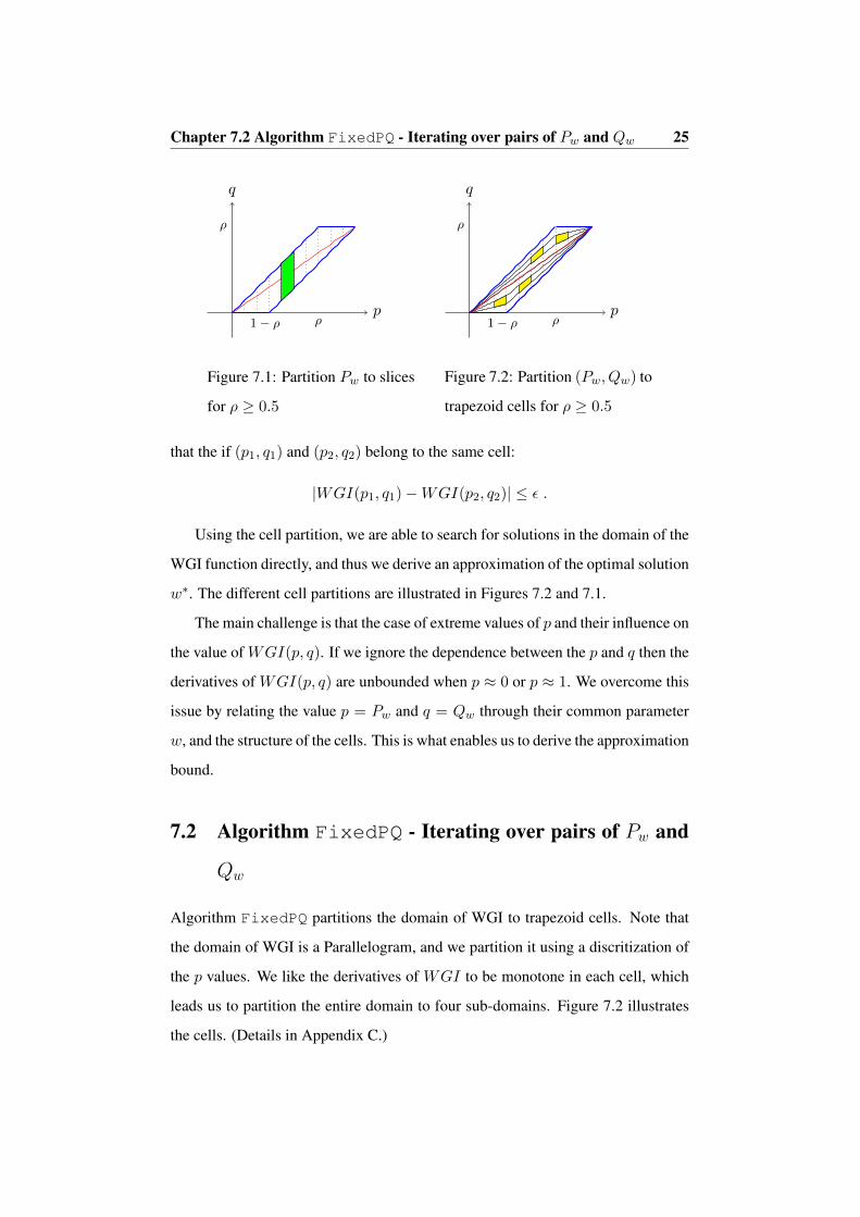
Chapter 7.2 Algorithm FixedPQ - Iterating over pairs of Pw and Qw 25
p
q
1− ρ ρ
ρ
Figure 7.1: Partition Pw to slices
for ρ ≥ 0.5
p
q
1− ρ ρ
ρ
Figure 7.2: Partition (Pw, Qw) to
trapezoid cells for ρ ≥ 0.5
that the if (p1, q1) and (p2, q2) belong to the same cell:
|WGI(p1, q1)−WGI(p2, q2)| ≤ ε .
Using the cell partition, we are able to search for solutions in the domain of the
WGI function directly, and thus we derive an approximation of the optimal solution
w∗. The different cell partitions are illustrated in Figures 7.2 and 7.1.
The main challenge is that the case of extreme values of p and their influence on
the value of WGI(p, q). If we ignore the dependence between the p and q then the
derivatives of WGI(p, q) are unbounded when p ≈ 0 or p ≈ 1. We overcome this
issue by relating the value p = Pw and q = Qw through their common parameter
w, and the structure of the cells. This is what enables us to derive the approximation
bound.
7.2 Algorithm FixedPQ - Iterating over pairs of Pw and
Qw
Algorithm FixedPQ partitions the domain of WGI to trapezoid cells. Note that
the domain of WGI is a Parallelogram, and we partition it using a discritization of
the p values. We like the derivatives of WGI to be monotone in each cell, which
leads us to partition the entire domain to four sub-domains. Figure 7.2 illustrates
the cells. (Details in Appendix C.)

Chapter 7.2 Algorithm FixedPQ - Iterating over pairs of Pw and Qw 26
Algorithm FixedPQ iterates over pairs of (p, q) which are the vertices of the
trapezoid cells. For each such pair its WGI(p, q) is evaluated, and the candidate
(p, q) pairs are sorted from the lowest WGI(p, q) to the highest. The sorted list
is then scanned until a feasible stochastic linear classifier with those parameters is
found, i.e., a weight vector w such that ‖w‖ ≤ 1 and p = Pw and q = Qw.
Notice that computing the value of WGI and testing the feasibility of a pair
(p, q) does not require the computation of the classifier w and can be done in O(1)
time. This follows since w = α~a + β~b, and given the values of α, β, ‖~a‖, ‖~b‖
and (~a ·~b) we can compute the norm of w directly from those values in O(1) time
without computing the weight vector w explicitly. Computing the weight vector w
requires O(d) time. In FixedPQ a weight vector w is computed only once - for
the first feasible candidate point (p, q) encountered in the scan.
The complexity Algorithm FixedPQ is O(Nd) + O(ε−2 log
(ε−1))
, where
O(Nd) is for computing ~a and ~b and the O(ε−2 log
(ε−1))
is for sorting O(ε−2)
candidate points.
Candidate generation: A list of (p, q) pairs is created by first selecting O(ε−1)
evenly spaced points that cover the feasible interval for Pw. The feasible interval
is a subsection of [0, 1] that is determined by the data (see Appendix D.4). We also
force points at p = ρ and p = 1 − ρ if these coincide the feasible interval. This
ensures that the cells generated are contained within a single sub-domain (more in
Appendix C).
Next, for each discretized value of p we define O(ε−1)
evenly spaced val-
ues of q in the following two intervals: from max (0, ρ+ p− 1) to ρp, and from
ρp to min (p, ρ). Finally, the pairs are filtered to include only feasible values (as
described in Appendix D.4). This process produces O(ε−2)
pairs.
Appendix E.1 provides pseudo-code, a correctness proof and complexity analysis
for FixedPQ.

Chapter 7.3 Algorithm FixedPSearchQ - Iterating over values Pw 27
7.3 Algorithm FixedPSearchQ - Iterating over values
Pw
Algorithm FixedPSearchQ iterates over values of p which are the endpoints
of mutually exclusive slices of trapezoid cells (more in Appendix C). A slice of
trapezoid cells, is the set of trapezoid cells which share the same p range (see
Figure 7.1). These endpoints are the candidates in this case, and for each candidate
at most two weight vector are computed. We filter the non-feasible points, and
return the classifier w for the point that achieves the lowest WGI.
Notice that since we do not have the q values in the candidate stage we cannot
compute the value WGI before computing a weight vector w or sort according to
the WGI values as we did in FixedPQ. Instead we must compute a weight vector
w for each candidate and return the best weight vector w. However, since we are
only interested in the minimum WGI there is no need to sort. The complexity of
this algorithm is O(Nd) +O(dε
).
Candidate generation: The candidates are p values that are generated by se-
lecting O(ε−1)
evenly spaced points that cover the feasible interval for Pw as in
FixedPQ. The main difference is that we do not discretize the q values, but main-
tain a complete slice of all feasible q values for a given range of p values. (More in
Appendix C).
Appendix E.2 provides pseudo-code, a correctness proof and complexity analysis
for FixedPSearchQ.
7.4 Algorithm DependentWGI - Dependent case
Algorithm DependentWGI describes the algorithm for the case where the con-
straints over Pw and Qw are dependent, i.e.,~b = λ~a. Appendix C.9, shows that the
optimal weight vector is w = ± ~a‖~a‖ , both attaining equal values of WGI. In order
to compute this weight vector, we compute ~a and normalize it in O(Nd) time. We

Chapter 7.5 Summary 28
also compute the WGI value in O(1) time. The total time complexity is O(Nd).
Appendix E.3 provides pseudo-code, a correctness proof and complexity analysis
for DependentWGI.
7.5 Summary
We distinguish between the case that ~a and ~b are linearly independent and the
case when they are linearly dependent. Algorithm DependentWGI finds the op-
timal solution for the case where ~a and~b are linearly dependent, while the remain-
ing two algorithms FixedPQ and FixedPSearchQ are for the linearly inde-
pendent case, each using a different search method. Algorithm FixedPQ iter-
ates over different possible values of (p, q) pairs and its complexity is: O(Nd) +
O(ε−2 log (ε−1)). Algorithm FixedPSearchQ iterates only over a p candidates,
and for each computes the optimal q value. The complexity of FixedPSearchQ
is: O(Nd) + O(dε
). The better running time depends on whether d is larger than
O(ε−1 log (ε−1)) or not.
Finally, if we assume algorithms DependentWGI, FixedPQ and
FixedPSearchQ find a weak learner in HI as described by the Weak Stochastic
Hypothesis Assumption 5.0.1 then we are able to boost the results using the DTL
algorithm using Theorem 5.0.1. Formally the following theorem holds:
Theorem 7.5.1. LetHI be the feasible stochastic linear classifiers over input space
X . Let γ ∈ (0, 0.5], and let f be any target function such that HI γ-satisfies the
Weak Stochastic Hypothesis Assumption with respect to f . Let D be any target
distribution, and let T be the tree generated by DTL(D, f,G, t) by using algo-
rithms DependentWGI, FixedPQ and FixedPSearchQ as the local oracles
for t iterations. Then for any target error ε, the error ε(T ) is less than ε provided
that:
t ≥(
1
ε
)c/(γ2ε2 log (1/ε))
if G(q) = 4q(1− q)

Chapter 8
Empirical Evaluation
8.1 Validating Strong Learnability
In this section we test our classifier in learning scenarios to verify it captures the
target function well. We demonstrate this ability with targets with increasing dif-
ficulty as well as unbalanced classes. All experiments were carried in the setting
of a 2-dimensional space on random unit size vectors. The reported results are the
average of 10 repetitions of each experiment, and the number of internal nodes in
the tree is 15 unless otherwise noted.
Single Hyperplane: In the first experiment the concept class is a hyperplane
which intersects the origin and both classes have equal weight. As figure 8.1 shows
the algorithm constantly selects hyperplanes which are very close to the target func-
tion, and indeed as a result the accuracy of the trained model is around 0.99 which
shows that the target is captured well.
Single Hyperplane and Artificial Bias: Next, we investigate the behavior when
we add a bias term to the classifier. We model the bias term by adding a constant-
valued feature to each example. We note that since the decision boundary intersects
the origin there is no reason to add this bias term, however, we want to examine the
29

Chapter 8.1 Validating Strong Learnability 30
Figure 8.1: Single Hyperplane Decisions
The decisions taken by the proposed classifier. The title explains the
position in the tree hierarchy (root is index 0). On the left the input
distribution s.t the circle size is relative to sample weight and the color
is based on the true label. On the right the decision of the internal node.

Chapter 8.1 Validating Strong Learnability 31
case where the classifier and the target are mismatched (in practice when the target
function is unknown it may be beneficial to use a bias in different scenarios).
Now, the data contains an artificial constant that the classifier should theoreti-
cally ignore. A-priori, we know it is possible to cancel the effect of the bias: both ~a
and~b will have their last coordinate to be the value of the bias, the decision in each
node of the tree - w is a linear combination of the form w = α~a + β~b. Therefore,
for the bias to be canceled out, the classifier needs to enforce α− β = 0.
In practice, we indeed see a trend of the classifier to reduce the last coordinate
to 0. However as shown in table 8.1, we also see a drop in the confidence when the
bias is increased. This phenomena is explained if we consider the limitations we
imposed on the stochastic linear classifier:
When the bias (denoted as b) is zero, the data vector x is exactly norm one
i.e 1 =∑x2i . Since the stochastic linear classifier is restricted to consider input
vectors of norm ≤ 1, once a bias b > 0 is introduced, all the true data coordinates
(xi) are normalized by a factor θb which is:
1 =∑
(θb · xi)2 + b2 → θb =1√
1 + b2
Denote xb andwb the data and the classifier if the data is modeled with bias b. Even
if we assume that ∀b : w0 = wb (the algorithm completely ignores the bias) we
still need to consider how the classifier output changes because of this added bias.
Denote by c = w0·x0+12 (the result of the prediction without bias) thus w0 · x0 =
2c− 1, the new prediction for bias b > 0 is
cb =wb · xb + 1
2=w0 · xb + 1
2=θb · w0 · x0 + 1
2= θb(c− 0.5) + 0.5
The first transition is because we assumed that w0 = wb.
The confidence is the distance cb − 0.5 and therefore for b is θb(c − 0.5) and
since θb < 1 we have that cb is always smaller than the confidence for bias 0 (which
is c − 0.5). In other words, even if we have the same stochastic linear classifier,
we lose a factor of θb in confidence due to the restriction ‖x‖ ≤ 1. We notice that
by weakening the restriction to ‖w · x‖ ≤ 1 we could have avoided the reduction

Chapter 8.1 Validating Strong Learnability 32
Table 8.1: Bias effects on confidenceb bias cb positive mean θb normalization coefficient
0 0.8 1
1 0.71 0.707
1.5 0.67 0.555
2 0.63 0.447
3 0.6 0.316
5 0.55 0.196
10 0.51 0.099
in confidence however it is unclear what effect it would have on our solution since
the optimization solved in Appendix D.1 will no longer hold.
Table 8.1 shows the drop in prediction confidence in the first internal node as
the bias changes. We note that in our tests the weight in the predictor that matched
the bias was reduced to almost 0. The middle column shows that the prediction
confidence was indeed reduced according to the relation described above.
Single Hyperplane with Unbalalnced Labels In the next test, we show strong
learnability even for unbalanced classes. For this experiment we changed the ratio
between classes from 1:1 we had in the previous experiments to 2:1 ratio between
the classes. We observed that our classifier’s accuracy dropped to 0.94. In order to
understand this drop we considered the first split of the tree. We noticed that even
though the accuracy dropped, when considering the soft accuracy i.e the average
of ‖yi − yi‖ we see that both the ”basic” balanced case and the unbalanced case
both consistently reach to scores around 0.3. We expected the soft accuracy value
to be comparatively low compared to the accuracy since we now care about the
confidence of the classification and not the sign. We know that the stochastic lin-
ear classifier could potentially reach perfect confidence but it is rarely achieved in
practice. Therefore the drop in accuracy is attributed to the fact that our classifier

Chapter 8.2 Comparison to other classifiers 33
tries to optimize the distances to the separating hyperplane and not the sign, but it
still preforms well in terms of accuracy (as it still scores accuracy of 0.94).
Multiple Hyperplanes - XOR In the next set of experiments the target function
is a XOR of the input hyperplanes (XOR is the product of the signs of w · x for
every w in the target function). We chose this type of targets, since our classifier is
an aggregation of linear decisions and should therefore capture this structure well.
In the first experiment we have two fixed hyperplanes. The reason the hyper-
planes are fixed is to make sure the classes are balanced. In the second experiment,
we again have two hyperplanes but now these are chosen randomly, which may
result in very unbalanced classes (for instance if the two hyperplanes lie very very
close to each other). In the last experiment we raise the number of hyperplanes to
three.
As expected, the accuracy goes down as the target becomes more complex: in
the first experiment the classifier has an accuracy of 0.94 while just changing to
unbalanced classes in the second experiment causes the accuracy to drop to 0.9.
The third experiment which has a more complex target achieves an initial accuracy
of 0.81. For the last experiment we also tested adding more internal splits, raising
the number of internal nodes from 15 (which we use as a default parameters) to
30 raises the accuracy to 0.9. Raising the number of nodes to 60 gives just 0.03
more to a total of 0.93. In general we see deceasing accuracy gains as we add more
nodes.
Finally, considering all the above experiments we can conclude that the pro-
posed classifier is able to capture these target concepts well (even non linear ones).
8.2 Comparison to other classifiers
This section discuss empirical evaluations of our classifier on synthetic data-sets we
created with the motivation of understanding the benefit of our decision tree using
stochastic linear classifiers, compared to decision tree with decision stumps, e.g.,

Chapter 8.2 Comparison to other classifiers 34
CART, and a standard linear classifier, e.g., linear SVM. We selected the simulated
data, with the goal of highlighting the similarities and differences between the
classifiers. In the following, we described the results of two simulated data sets.
In the first experiment we demonstrate that unlike standard decision tree algo-
rithms, our method fits well a data-set which is labeled according a random linear
boundary with noise in a high dimension. Specifically, we select a random hy-
perplane w and each sample x are random unit vectors, where the the label is
y = sign(w · x) and dimension is d = 100. We add random classification noise,
i.e., flip the label with probability of θ. We show the accuracy of our model com-
pared to both CART and linear SVM as a function of the noise rate θ in Figure
8.2. Clearly, SVM is ideal for this task, and indeed it outperforms the other two
classifiers. We ran both CART and our method to build decision trees of depth 10.
The results show that our method achieves competitive performance to SVM while
outperforming CART.
The second synthetic data set demonstrates the ability of our classifier to handle
non-linearly separable examples, where the boundaries are not axis aligned. Again,
all samples are random unit vectors of dimension d. The labels correspond to
the XOR of the samples with two hyperplanes, which are perpendicular to each
other and are not axis aligned. Specifically we take w1 = [~1d/2,~1d/2] and w2 =
[ ~−1d/2,~1d/2] and the label is y = sign(x ·w1)⊕ sign(x ·w2). Both decision trees
were allowed to reach depth of 10 and the sample size is 10, 000. We used various
dimension sizes from d = 6 to d = 30, and the results are plotted in Figure 8.3.
The results were in line with out intuition. First, Linear SVM achieves the
worst performance since it does not have the expressive power required for rep-
resenting this target function. Second, a decision tree algorithm, such as CART,
which considers only a single attribute in each split, requires a significant depth
to approximate this high-dimensional XOR. Finally, our method achieves a good
accuracy since it is not limited to a single hyperplane, as is Linear SVM, nor is it
limited to axis aligned decisions, as is CART. We do note, that since our method

Chapter 8.3 Real Data-sets 35
0
0.1
0.2
0.3
0.4
0.5
0.6
0.7
0.8
0.9
1
0 0.1 0.2 0.3
Acc
ura
cy
Noise
decision tree stochastic tree linear SVM
Figure 8.2: Hyperplane with
noise.
Accuracy of the different classifiers
for linearly separable points. In or-
ange, our stochastic classifier, blue
is CART and grey is linear SVM.
5 10 15 20 25 30
dimensions
0.50
0.55
0.60
0.65
0.70
0.75
acc
ura
cy
linear SVM
stochastic tree
regular tree
Figure 8.3: Multi-dimensional
XOR
Unit vectors with norm 1, are la-
beled according to a multi dimen-
sional non-axis aligned XOR. Our
stochastic classifier (green) achieves
much higher accuracy than both a
linear SVM (blue) and CART (red).
is stochastic, we need to continuously repeat a hyperplane in order to make a split
more significant. This explains why, due to the limited depth of the decision tree,
our performance deteriorate as the dimension increases. An alternative is to limit
the number of nodes in the decision tree. Further experiments show that our method
can achieve the above performance with only 50 internal nodes (rather than a depth
of size 10, which implies 1024 internal nodes).
8.3 Real Data-sets
We show the performance of our classifier compared to Linear SVM and CART
on three data-sets that were taken from UCI dataset repository [Lic13]. The first
dataset Promoters contains 106 examples with 57 categorical features and two
classes. Since our algorithm runs on numeric data we encode each feature to it’s
one-hot representation for a total of 228 numerical features. The second dataset is
the Heart Disease Data Set which contains 303 samples with 13 numeric features.
In the original data there are 74 features, but it is common to use the above subset

Chapter 8.3 Real Data-sets 36
of features. The original data contains one negative class to indicate no disease
in the patient, and 4 positive classes each corresponding to a certain disease. We
reduced the problem to a positive vs. negative classification, by combining all the
diseases to one class. The third dataset Statlog (Heart) Data Set, has the same for-
mat as the previous only the target variable is already in binary format. There are
13 features and 270 samples in this dataset.
The following table shows the accuracy of all three classifiers used in our ex-
periments, and demonstrates the advantage of our proposed method:
Dataset CART Linear SVM Stochastic Tree
Promoters 0.8 0.87 0.91
Heart Disease Data Set 0.7 0.73 0.77
Statlog (Heart) Data Set 0.83 0.78 0.85
We note that we gave the same depth restriction to CART and our Stochastic
Decision Tree, however, our method seems sometimes to require a smaller depth to
converge. For the Promoters data-set, while CART was still improving at depth 10,
while the stochastic tree only needed only a depth of 3 to converge. This along with
the comparatively strong result of the Linear SVM may hint that the true decision
boundary can be approximated well with a hyperplane which is not axis aligned.
For the other two data-sets, Heart Disease Data Set and Statlog (Heart) Data Set
both methods converged at the same depth of 3 and 5 correspondingly.

Chapter 9
Conclusion
In this work we introduced a stochastic decision tree learning algorithm based on
stochastic linear classifiers. The main advantage of our approach is that it allows
the internal splits in the node to have a global effect, on the one hand, and we
can efficiently minimize the Gini index, on the other hand. From a theoretical
perspective, we are able to maintain the basic decision tree learning result under
the assumption of weak learning.
Our empirical finding are encouraging, and suggest doing a more comprehen-
sive empirical analysis of the strengths and weaknesses of our method. Another
possible research direction would be to explore the benefits of the stochastic linear
classifier in other boosting frameworks such as AdaBoost.
From a more theoretical perspective we hope to extend our method to work
efficiently for a large class splitting functions, under minimal assumptions on this
class.
Another challenging research direction, is to change the linear modeling for
Pr (y|x) to a more complex representation, such as a log linear model. This gives
rise to an immediate computational challenge of efficiently minimizing the splitting
criteria.
37

Bibliography
[ABF+08] Michael Alekhnovich, Mark Braverman, Vitaly Feldman, Adam R.
Klivans, and Toniann Pitassi. The complexity of properly learning
simple concept classes. J. Comput. Syst. Sci., 74(1):16–34, 2008.
[BB98] Kristin P Bennett and Jennifer A Blue. A support vector machine
approach to decision trees. In Neural Networks Proceedings, 1998.
IEEE World Congress on Computational Intelligence. The 1998 IEEE
International Joint Conference on, volume 3, pages 2396–2401.
IEEE, 1998.
[BFSO84] Leo Breiman, Jerome Friedman, Charles J Stone, and Richard A Ol-
shen. Classification and regression trees. CRC press, 1984.
[BR93] Avrim Blum and Ronald L. Rivest. Training a 3-node neural network
is NP-Complete. In Machine Learning: From Theory to Applications
- Cooperative Research at Siemens and MIT, pages 9–28, 1993.
[CK03] Erick Cantu-Paz and Chandrika Kamath. Inducing oblique decision
trees with evolutionary algorithms. IEEE Trans. Evolutionary Com-
putation, 7(1):54–68, 2003.
[FAB08] Janis Fehr, Karina Zapien Arreola, and Hans Burkhardt. Fast support
vector machine classification of very large datasets. In Data Analysis,
Machine Learning and Applications, pages 11–18. Springer, 2008.
38

BIBLIOGRAPHY 39
[GMD13] Dejan Gjorgjevikj, Gjorgji Madjarov, and Saso Dzeroski. Hybrid de-
cision tree architecture utilizing local svms for efficient multi-label
learning. International Journal of Pattern Recognition and Artificial
Intelligence, 27(07):1351004, 2013.
[HKS93] David Heath, Simon Kasif, and Steven Salzberg. Induction of oblique
decision trees. Journal of Artificial Intelligence Research, 2(2):1–32,
1993.
[KM99] Michael J. Kearns and Yishay Mansour. On the boosting ability of
top-down decision tree learning algorithms. J. Comput. Syst. Sci.,
58(1):109–128, 1999.
[Lic13] M. Lichman. UCI machine learning repository, 2013.
[MKS94] Sreerama K. Murthy, Simon Kasif, and Steven Salzberg. A system for
induction of oblique decision trees. Journal of artificial intelligence
research, 1994.
[Qui86] J. R. Quinlan. Induction of decision trees. Machine Learning, 1:81–
106, 1986.
[Qui93] J Ross Quinlan. C4. 5: Programming for machine learning. Morgan
Kauffmann, page 38, 1993.
[RLSCH12] Irene Rodriguez-Lujan, Carlos Santa Cruz, and Ramon Huerta.
Hierarchical linear support vector machine. Pattern Recognition,
45(12):4414–4427, 2012.
[Sch90] Robert E Schapire. The strength of weak learnability. Machine learn-
ing, 5(2):197–227, 1990.
[WRR+16] D.C. Wickramarachchi, B.L. Robertson, M. Reale, C.J. Price, and
J. Brown. Hhcart. Comput. Stat. Data Anal., 96(C):12–23, April
2016.

Appendix A
Decision tree learning algorithm:
pseudo code
The pseudo code of Algorithm 1 encapsulates most existing decision tree learning
(DTL) algorithm, including algorithms such as CART by [BFSO84] and C4.5 by
[Qui93]. Our exposition of the decision tree algorithms tries to abstract the specific
splitting function G and the way to minimize it. We also generalize the standard
framework to handle stochastic classifiers. We start with describing the oracles we
assume.
The first oracle minimizes the splitting criteria for a hypothesis in an internal
node. The function FitHI(S,D,G) receives as input a sample S, and a distri-
bution D over the sample S and a splitting criteria G. It returns (h∗, g∗) where
h∗ ∈ HI is the hypothesis that minimizes the splitting criteria G over the distribu-
tion D on S and g∗ is its reduction in the value of the splitting criteria G.
The second oracle FitHL(S,D) receives as input a sample S, a distribution
D over the sample S and returns a hypothesis h ∈ HL which minimizes the error
(and not the splitting criteria G).
We have a function SplitLeaf(T, l, h) which receives a decision tree T , a leaf
l ∈ Leaves(T ), a hypothesis h ∈ HI and returns a new tree where we split leaf l
using hypothesis h.
40

Chapter. A: Decision tree learning algorithm: pseudo code 41
The decision tree learning algorithm runs t iterations. In each iteration, for each
leaf l ∈ Leaves(T ) the function FitHI evaluates the optimal predictor h∗l for the
leaf l along with g∗l , the local reduction in G induced by h∗l . The local reduction
is weighted by wl to obtain the global reduction in G, i.e., wlg∗l , and we select the
leaf that minimizes G globally. We update the tree by splitting this leaf, and for
the new leaves update the probabilities of inputs to reach each of them. Once t
iterations are done and the leaves have been determined, FitHL selects for each
leaf a predictor from HL by minimizing the error (and not the splitting criteria G).
One can observe that our framework encapsulates common decision tree method-
ologies algorithms, such as C4.5 and CART, as follows:
1. HI is the family of all decision stumps and HL = {0, 1}.
2. The function FitHI is implemented by evaluating all the decision stumps
and selecting the best according to G.
3. The function FitHL sets y = 0 or y = 1 according to the majority class in
the leaf, minimizing the error given a constant label predictor
We presented a general basic scheme of the DTL algorithm. We did not de-
scribe other hyperparameters (such as minimal split size) or methods to refine the
model (such as pruning) which could be applied to the generic algorithm in order
to improve results. Our goal is to focus of the core properties of the DTL which
we believe are well represented in our framework.

Chapter. A: Decision tree learning algorithm: pseudo code 42
Algorithm DTL(S - sample, G splitting criteria, t number of iterations)
1 Initialize T to be a single-leaf tree with node r, for x ∈ S: pr(x) = 1|S| ,
wr = 1, and qr = |{x∈S:f(x)=1}||S| .
2 while |Leaves(T )| < t do
3 ∆best ← 0; bestl ← ⊥; besth ← ⊥
4 for each l ∈ Leaves(T ): do
5 h∗l , g∗l ← FitHI(S,
1wlpl(x), G)
6 ∆l ← wlG(ql)− wl · g∗l7 if ∆l ≥ ∆best then
8 ∆best ← ∆l; bestl ← l; besth ← h∗l
end
end
9 for x ∈ S do
10 pl1(x)← pl(x) · Pr (besth(x))
11 pl0(x)← pl(x) · (1− Pr (besth(x)))
end
12 wl1 ←∑
x∈S pl1(x); wl0 ←∑
x∈S pl0(x)
13 ql1 ←∑
x∈S:f(x)=1 pl1(x); ql0 ←∑
x∈S:f(x)=1 pl0(x)
14 T ← SplitLeaf(T, bestl, besth)
end
15 for each l ∈ leaves(T ): dohl ← FitHL(S, 1
wlpl(x))
end
16 return TAlgorithm 1: Decision tree learning algorithm

Appendix B
Proof of Theorem 5.0.1
In this section we provide a sketch of the proof for Theorem 5.0.1 under the
Stochastic Weak Learning Assumption. The proof is based on the proof for the
deterministic case by [KM99], however it is slightly modified to account for the
stochastic hypothesis we introduce in this work. We will only prove the place
where the proofs differ, namely Lemma 2 of [KM99] is substitute by Lemma B.0.1.
We start with a few notations. Let f be the target function, let T be a decision
tree, a leaf l ∈ Leaves(T ), and let h ∈ HI . Denote the leaves introduced by
Split(T, l, h) by l1 and l0. Recall that purity(l) is the fraction of positive exam-
ples that reach leaf l from all of the examples that reach it. We use the following
shorthand notations for reoccurring expressions:
q =purity(l), p = purity(l0), r = purity(l1)
τ = Pr(x,y)∼D
(Reach(x, l1)|Reach(x, l))
= Pr(x,y)∼D
(h(x) = 1|Reach(x, l))
=weight(l1)
weight(l)
Since q = (1 − τ)p + τr and τ ∈ [0, 1] than without loss of generality we have:
p ≤ q ≤ r. Let:
δ = r − p .
43

Chapter. B: Proof of Theorem 5.0.1 44
Let Dl be the distribution over input at leaf l. We also define D′l the balanced
distribution over inputs in leaf l in which the probability positive (or negative)
weights is 1/2. Formally,
Dl(x) =Reach(x, l)
weight(l)D(x)
D′l(x) =
Dl(x)
2q if f(x) = 1
Dl(x)2(1−q) if f(x) = 0
Recall that the information gain is ∆ = G(q) − (1 − τ)G(p) − τG(r). Note
that if either δ is small or τ is near 0 or 1 then the information gain is small.
Lemma B.0.1 shows that if h ∈ HI is used to split at l, and h satisfies the Weak
Stochastic Hypothesis Assumption for D′l, then both δ cannot be too small, and τ
cannot be too close to either 0 or 1.
Lemma B.0.1. Let p, τ and δ be as defined above for the split h ∈ HI at leaf l.
Let Dl and D′l also be defined as above for l. If the function h satisfies
Prx∼D′l (h(x) 6= f(x)) ≤ 0.5− γ, Then:
τ(1− τ)δ ≥ 2γq(1− q) .
Proof. We calculate the following expressions in terms of τ, r and q:
Prx∼Dl
(f(x) = 1, h(x) = 1) = τr
Therefore,
Prx∼Dl
(f(x) = 0, h(x) = 1) = τ(1− r)
and
Prx∼Dl
(f(x) = 1, h(x) = 0) = (1− τ)p = q − τr
Next we consider the error terms under the distribution D′l. When changing from
the distribution Dl to D′l we need to scale the expression according to the labels:
Prx∼D′l
(f(x) = 0, h(x) = 1) =τ(1− r)2(1− q)

Chapter. B: Proof of Theorem 5.0.1 45
and
Prx∼D′l
(f(x) = 1, h(x) = 0) =q − rτ
2q
Finally the error terms are combined to achieve the total error:
Prx∼D′l
(f(x) 6= h(x)) = Prx∼D′l
(f(x) = 0, h(x) = 1) + Prx∼D′l
(f(x) = 1, h(x) = 0)
=τ(1− r)2(1− q)
+q − rτ
2q=
1
2+τ
2
(1− r1− q
− r
q
)=
1
2+τ
2· q − rq(1− q)
By our assumption on h we have,
Prx∼D′l
(f(x) 6= h(x)) =1
2+τ
2· q − rq(1− q)
≤ 1
2− γ
which implies thatτ
2· r − qq(1− q)
≥ γ
Substituting r = q + (1− τ)δ we get:
τ
2· (1− τ)δ
q(1− q)≥ γ → τ(1− τ)δ ≥ 2γq(1− q)
as required.

Appendix C
Bounding the WGI by regions
In this appendix, we show how to partition the domain of WGI into cells such that
the difference between values of the WGI of points in the same cell is bounded by
ε. Namely, we prove the following theorem.
Theorem 7.1.1. Given data distribution Dl which has a positive label probability
of ρ and a parameter ε ∈ (0, 1) it is possible to partition the domain of WGI:
{(p, q)|0 ≤ p ≤ 1,max (0, ρ+ p− 1) ≤ q ≤ min (ρ, p)} into O(ε−2)
cells, such
that the if (p1, q1) and (p2, q2) belong to the same cell:
|WGI(p1, q1)−WGI(p2, q2)| ≤ ε .
C.1 Partitioning the WGI to monotone regions
Consider the domain of WGI which is
R = {(p, q)|p ∈ (0, 1), q ∈ [max (0, p+ ρ− 1),min (ρ, p)]} .
Note that the values of p = 0 and p = 1 are not included. We discuss and add them
in Section C.7. We partition R to two sub-domains using the line q = ρp, namely,
Ra = {(p, q)|p ∈ (0, 1), q ∈ [ρp,min (ρ, p)]}
46

Chapter C.1 Partitioning the WGI to monotone regions 47
and
Rb = {(p, q)|p ∈ (0, 1), q ∈ [max(0, p+ ρ− 1), ρp]} ,
as illustrated in Figure C.1.
We show that the function WGI is monotone in each of those domains.
Lemma C.1.1. Given data distribution Dl which has a positive class weight of ρ,
the WGI function:
WGI(p, q) = 4
(ρ− q2
p− (ρ− q)2
1− p
)is monotone in both p and q in both Ra and Rb. Specifically, in Ra it is increasing
in p and decreasing in q and in Rb it is decreasing in p and increasing in q.
Proof. Since we are interested only in monotonicity, we can consider simply the
function g(p, q) = − q2
p −(ρ−q)2
1−p . In order to show that g(p, q) is monotone, we
first consider where its derivatives vanishes. The derivative with respect to q is
∂g(p, q)
∂q=− 2q
p+
2(ρ− q)(1− p)
=2(ρp− q)p(1− p)
This implies that the derivative vanishes at q = ρp which is the boundary of the
sub-domainsRa andRb, and hence g(p, q) is monotone in q in each of the domains.
Also, in Ra, since q > pρ, the derivative is negative and in Rb, since q ≤ pρ, it is
positive.
Next we consider the derivative with respect to p,
∂g(p, q)
∂p=q2
p2− (ρ− q)2
(1− p)2=
(q − ρp)(q(1− 2p) + ρp)
p2(1− p)2
This implies that the derivative vanishes at q = ρp and q = ρp2p−1 . The line q = ρp
is a boundary of our regions and so we consider only the other curve.
For p ∈ (0, 0.5) we have 1 − 2p > 0. This implies that q(1 − 2p) + ρp > 0.
Since q > ρp in Ra it implies that g(p, q) is increasing there, and similarly, since
q ≤ pρ, it is decreasing in Rb.
For p ∈ (0.5, 1) we have −1 < 1 − 2p < 0. For Rb, since q ≤ ρp we have
that q(1 − 2p) + ρp > 0 and hence g(p, q) is decreasing in p. For Ra, we have

Chapter C.2 Overview of the partition to cells 48
p
q
Ra
Rb
0.51− ρ ρ
ρ
Figure C.1: The domain R and the sub-domains Ra and Rb (for ρ ≥ 0.5)
p
q
1− ρ ρ
ρRa,r
Ra,l
Rb,r
Rb,l
Figure C.2: WGI: partitioned into regions for ρ ≥ 0.5
q ≤ p+ ρ− 1. This implies that q(1− 2p) + ρp ≤ (1− p)(2p− 1 + ρ) which is
non-negative since p ∈ (0.5, 1). Therefore q(p, q) is increasing in Ra.
Finally, for p = 0.5 we have that ∂g(p,q)∂p = (q−ρ/2)(ρ/2)1/16 which is positive in Ra
and negative in Rb as required.
Figure C.1 show pictorially the regions Ra and Rb.
C.2 Overview of the partition to cells
We partitioned the domain R of WGI to two sub-domains Ra and Rb. According
to Theorem C.1.1 in each of the sub-domains the WGI is monotone in p and q.
We will partition each sub-domain in two thus creating four regions with linear
boundaries which are monotone in p and q. Finally we partition each of the four
regions further into cells in order to bound the WGI difference as required.

Chapter C.3 First region: Rb,l 49
We first consider the difference in the value of WGI between two points:
|WGI(p1, q1)−WGI(p2, q2)| = 4
∣∣∣∣q22
p2+
(ρ− q2)2
1− p2− q2
1
p1− (ρ− q1)2
1− p1
∣∣∣∣≤ 4
∣∣∣∣q22
p2− q2
1
p1
∣∣∣∣+ 4
∣∣∣∣(ρ− q2)2
1− p2− (ρ− q1)2
1− p1
∣∣∣∣= 4∆1 + 4∆2 (C.1)
where ∆1 =∣∣∣ q22p2 − q21
p1
∣∣∣ and ∆2 =∣∣∣ (ρ−q2)2
1−p2 −(ρ−q1)2
1−p1
∣∣∣.We are going to consider the case where ρ ≥ 0.5. The symmetric case of
ρ < 0.5 can be reduced to this case by switching the labels and deriving the same
bound. For the definition of the cells we use the parameters ε ∈ (0, 1) which
controls the cell’s size.
We next present an analysis for each of four sub-domains, and show that in each
both ∆1 = O(ε) and ∆2 = O(ε). In addition each sub-domain will be partitioned
in to O(ε−2) cells.
C.3 First region: Rb,l
LetRb,l = {(p, q)|0 < p ≤ 1− ρ, 0 ≤ q ≤ ρp}. ClearlyRb,l ⊆ Rb, and by Lemma C.1.1
we know that WGI is decreasing in p and increasing in q in Rb,l.
We are now ready to define the cells. The cells will have two parameters pc ∈
(0, 1− ρ− ε] and α ∈ [ε, 1]. Let
cellRb,l(pc, α) = {(p, q)|pc ≤ p ≤ pc + ε, (α− ε)ρp ≤ q ≤ αρp} .
The cells would have pc = iε, for 0 ≤ i ≤ 1−ρε − 1 and α = jε, for 1 ≤ j ≤ 1/ε.
This implies that there are O(ε−2) cells in Rb,l. Since in Rb,l we have ∂WGI∂q ≥ 0,
there are p1, p2 ∈ (0, 1 − ρ], such that the maximum WGI value in cellRb,l(pc, α)
is obtained at a point (p1, q1) = (p1, αρp1) and the minimum value at (p2, q2) =
(p2, (α− ε)ρp2).
Chapter C.4 Second region: Rb,r 50
We bound ∆1 as follows:
∆1 =
∣∣∣∣q22
p2− q2
1
p1
∣∣∣∣ =
∣∣∣∣(α− ε)2ρ2p22
p2− α2ρ2p2
1
p1
∣∣∣∣≤ρ2(α2
≤ε︷ ︸︸ ︷|p2 − p1|+εp2
≤1︷ ︸︸ ︷|ε− 1|) ≤ ρ2(α2ε+ εp2) ≤ 2ε (C.2)
and ∆2 as follows,
∆2 =
∣∣∣∣(ρ− q2)2
1− p2− (ρ− q1)2
1− p1
∣∣∣∣ =
∣∣∣∣(ρ− (α− ε)ρp2)2
1− p2− (ρ− αρp1)2
1− p1
∣∣∣∣=ρ2
∣∣∣∣(1− (α− ε)p2)2
1− p2− (1− αp1)2
1− p1
∣∣∣∣=ρ2
∣∣∣∣((1− p2) + ((1− α) + ε)p2)2
1− p2− ((1− p1) + (1− α)p1)2
1− p1
∣∣∣∣≤ρ2
|p2 − p1|+ 2(1− α)|p2 − p1|+ 2p2ε+ (1− α)2
∣∣∣∣ p22
1− p2− p2
1
1− p1
∣∣∣∣+p2
2ε(
≤2︷ ︸︸ ︷1− α+ ε)
1− p2
≤5ε+ 2ε
p2
1− p2+ ρ2
∣∣∣∣p22 − p2
1 + p21p2 − p1p
22
(1− p1)(1− p2)
∣∣∣∣≤7ε+ ρ2
≤2︷ ︸︸ ︷(p1 + p2) |p2 − p1|(1− p1)(1− p2)
+ ρ2
≤1︷︸︸︷p1p2 |p2 − p1|
(1− p1)(1− p2)
≤7ε+ 3ερ2
(1− p1)(1− p2)
=10ε (C.3)
where we used the fact that ρ ≤ 1 and p ≤ 1 − ρ ≤ ρ ≤ 1 − p (or p1−p ≤ 1 or
ρ1−p ≤ 1).
Combining the bounds in (C.1), (C.2) and (C.3) the error for in each cell inRb,l
is bounded by 4(2ε+ 10ε) = 48ε.
C.4 Second region: Rb,r
Let Rb,r = {(p, q)|1− ρ ≤ p < 1, p+ ρ− 1 ≤ q ≤ ρp}. Clearly Rb,r ⊆ Rb, and
by Lemma C.1.1 we know that WGI is decreasing in p and increasing in q in Rb,r.

Chapter C.4 Second region: Rb,r 51
We are now ready to define the cells. The cells will have two parameters pc ∈
[1− ρ, 1− ε) and α ∈ [ε, 1]. Let
cellRb,r(pc, α) ={(p, q) : pc ≤ p ≤ pc + ε,
(α− ε)ρp+ (1− α+ ε)(p+ ρ− 1) ≤ q ≤ αρp+ (1− α)(p+ ρ− 1)} .
The cells would have pc = iε, for (1 − ρ)/ε ≤ i ≤ 1/ε − 1 and α = jε, for
1 ≤ j ≤ 1/ε. This implies that there are O(ε−2) cells in Rb,r. Since in Rb,r we
have ∂WGI∂q ≥ 0, there are p1, p2 ∈ [1 − ρ, 1), such that the maximum WGI value
in cellRb,r(pc, α) is obtained at a point (p1, q1) = (p1, αρp1 +(1−α)(p1 +ρ−1))
and the minimum value at (p2, q2) = (p2, (α− ε)ρp2 + (1− α+ ε)(p2 + ρ− 1))
We bound ∆1 as follows:
∆1 =
∣∣∣∣q22
p2− q2
1
p1
∣∣∣∣=
∣∣∣∣((α− ε)ρp2 + (1− α+ ε)(p2 + ρ− 1))2
p2− (αρp1 + (1− α)(p1 + ρ− 1))2
p1
∣∣∣∣≤α2ρ2 |p2 − p1|+ ε
≤2︷ ︸︸ ︷|ε− 2α| ρ2p2 + 2
≤0.25︷ ︸︸ ︷α(1− α) ρ |p2 − p1|
+ 2ε
≤1︷ ︸︸ ︷|2α− ε− 1| ρ
≤1︷ ︸︸ ︷|p2 + ρ− 1|+
(1− α)2
∣∣∣∣(p2 + ρ− 1)2
p2− (p1 + ρ− 1)2
p1
∣∣∣∣+ε
≤2︷ ︸︸ ︷|2− 2α+ ε|(p2 + ρ− 1)2
p2
≤5.5ε+
C.5︷ ︸︸ ︷∣∣∣∣(p2 + ρ− 1)2
p2− (p1 + ρ− 1)2
p1
∣∣∣∣+C.6︷ ︸︸ ︷
2ε(p2 + ρ− 1)2
p2≤ 12.5ε
(C.4)
Where we used the following expressions:∣∣∣∣(p2 + ρ− 1)2
p2− (p1 + ρ− 1)2
p1
∣∣∣∣ ≤ |p2 − p1|+ (ρ− 1)2 |p1 − p2|p1p2
≤ 2ε (C.5)
Chapter C.5 Third region Ra,l 52
2ε(p2 + ρ− 1)2
p2≤2ε
p2 + 2
≤0.5︷ ︸︸ ︷|ρ− 1|+(ρ− 1)2
p2
≤2ε
2 +
≤0.5︷ ︸︸ ︷(1− ρ)
1− ρp2
≤5ε (C.6)
where we used the fact that p ≥ 1− ρ (or 1−ρp ≤ 1).
For ∆2 we have
∆2 =
∣∣∣∣(ρ− q2)2
1− p2− (ρ− q1)2
1− p1
∣∣∣∣=
∣∣∣∣(ρ− (α− ε)ρp2 − (1− α+ ε)(p2 + ρ− 1))2
1− p2− (ρ− αρp1 − (1− α)(p1 + ρ− 1))2
1− p1
∣∣∣∣≤ |p1 − p2|
≤1︷︸︸︷ρ2α2 +2ρ
≤0.25︷ ︸︸ ︷α(1− α) +
≤1︷ ︸︸ ︷(1− α)2
+
≤1︷ ︸︸ ︷(1− p2)
ρ2ε
≤2︷ ︸︸ ︷|ε− 2α|+2ρε
≤1︷ ︸︸ ︷|2α− 1− ε|+ε
≤2︷ ︸︸ ︷|2− 2α+ ε|
≤8.5ε (C.7)
Combining the bounds in (C.1), (C.4) and (C.7) the error for in each cell inRb,l
is bounded by 4(12.5ε+ 8.5ε) = 84ε.
C.5 Third region Ra,l
LetRa,l = {(p, q)|0 < p ≤ ρ, ρp ≤ q ≤ p}. ClearlyRa,l ⊆ Ra, and by Lemma C.1.1
we know that WGI is increasing in p and decreasing in q in Ra,l.
We are now ready to define the cells. The cells will have two parameters pc ∈
(0, ρ− ε] and α ∈ [ε, 1]. Let
cellRa,l(pc, α) = {(p, q)|pc ≤ p ≤ pc + ε, (α− ε)p+ (1− α+ ε)ρp ≤ q ≤ αp+ (1− α)ρp} .
The cells would have pc = iε, for 0 ≤ i ≤ ρ/ε − 1 and α = jε, for 1 ≤ j ≤ 1/ε.
This implies that there are O(ε−2) cells in Ra,l. Since in Ra,l we have ∂WGI∂q ≤ 0,

Chapter C.6 Fourth region Ra,r 53
there are p1, p2 ∈ (0, ρ], such that the maximum WGI value in cellRa,l(pc, α) is
obtained at a point (p1, q1) = (p1, (α− ε)p1 + (1− α+ ε)ρp1) and the minimum
value at (p2, q2) = (p2, αp2 + (1− α)ρp2)
We bound ∆1 as follows,
∆1 =
∣∣∣∣q22
p2− q2
1
p1
∣∣∣∣ =
∣∣∣∣(αp2 + (1− α)ρp2)2
p2− ((α− ε)p1 + (1− α+ ε)ρp1)2
p1
∣∣∣∣≤ |p2 − p1| |ρ+ (1− ρ)α|2 + 2εp1 |ρ+ (1− ρ)α| |ρ− 1|+ ε2p1(ρ− 1)2
≤4ε (C.8)
Where we used:
|ρ+ α(1− ρ)| ≤ |ρ|+ α |1− ρ|α≤1≤ |ρ|+ |1− ρ| 0≤ρ≤1
= ρ+ 1− ρ = 1
and bound ∆2 as follows,
∆2 =
∣∣∣∣(ρ− q2)2
1− p2− (ρ− q1)2
1− p1
∣∣∣∣=
∣∣∣∣(ρ− αp2 − (1− α)ρp2)2
1− p2− (ρ− (α− ε)p1 − (1− (α− ε))ρp1)2
1− p1
∣∣∣∣≤ρ2 |p1 − p2|+ 2α |ρ(ρ− 1)| |p2 − p1|+ α2(1− ρ)2
∣∣∣∣ p22
1− p2− p2
1
1− p1
∣∣∣∣+2εp1(1− ρ) |ρ− αp1 − (1− α)ρp1|
1− p1+ε2p2
1(1− ρ)2
1− p1
≤8.5ε (C.9)
Combining the bounds in (C.1), (C.8) and (C.9) the error for in each cell in
Ra,l is bounded by 4(4ε+ 8.5ε) = 50ε.
C.6 Fourth region Ra,r
LetRa,r = {(p, q)|ρ ≤ p < 1, ρp ≤ q ≤ ρ}. ClearlyRa,r ⊆ Ra, and by Lemma C.1.1
we know that WGI is increasing in p and decreasing in q in Ra,r.
We are now ready to define the cells. The cells will have two parameters pc ∈
[1− ρ, 1− ε) and α ∈ [ε, 1]. Let
cellRa,r(pc, α) = {(p, q)|pc ≤ p ≤ pc + ε, (α− ε)ρ+ (1− α+ ε)ρp ≤ q ≤ αρ+ (1− α)ρp} .

Chapter C.7 WGI is continuous in p = 0 and p = 1 54
The cells would have pc = iε, for ρ/ε ≤ i ≤ 1/ε− 1 and α = jε, for 1 ≤ j ≤ 1/ε.
This implies that there are O(ε−2) cells in Ra,r. Since in Ra,r we have ∂WGI∂q ≤ 0,
there are p1, p2 ∈ [1− ρ, 1), such that the maximum WGI value in cellRa,r(pc, α)
is obtained at a point (p1, q1) = (p1, (α− ε)ρ+ (1−α+ ε)ρp1) and the minimum
value at (p2, q2) = (p2, αρ+ (1− α)ρp2)
We bound ∆1 as follows,
∆1 =
∣∣∣∣q22
p2− q2
1
p1
∣∣∣∣ =
∣∣∣∣(αρ+ (1− α)ρp2)2
p2− ((α− ε)ρ+ (1− α+ ε)ρp1)2
p1
∣∣∣∣≤ρ2 (|p2 − p1|+ 2α |p1 − p2|+ 2ε |1− p1|)
+ ρ2
∣∣∣∣α2(1− p2)2
p2− α2(1− p1)2
p1− ε(ε− 2α)(1− p1)2
p1
∣∣∣∣≤8ε (C.10)
and ∆2 as follows,
∆2 =
∣∣∣∣(ρ− q2)2
1− p2− (ρ− q1)2
1− p1
∣∣∣∣=
∣∣∣∣(ρ− αρ− (1− α)ρp2)2
1− p2− (ρ− (α− ε)ρ− (1− (α− ε))ρp1)2
1− p1
∣∣∣∣≤ρ2(1− α)2 |p1 − p2|+ ρ2ε |2− 2α+ ε| (1− p1)
≤3ε (C.11)
Combining the bounds in (C.1), (C.10) and (C.11) the error for in each cell in
Ra,r is bounded by 4(8ε+ 3ε) = 44ε.
C.7 WGI is continuous in p = 0 and p = 1
We show that the value of WGI is continuous at both extreme points p = 0 and
p = 1 for point (p, q) ∈ R. Namely, we show that its value is 4ρ(1− ρ). This will
allow us to extend the sub-domains from p ∈ (0, 1) to p ∈ [0, 1]. Recall that,
WGI(p, q) = 4
(ρ− q2
p− (ρ− q)2
1− p
)

Chapter C.7 WGI is continuous in p = 0 and p = 1 55
Lemma C.7.1. WGI(p, q) (7.1) is continuous in p = 0.
Proof. By definition of WGI 7.1, we know thatWGI(0, q) = 4ρ(1−ρ). We show
that this is also the limit when p approaches 0.
limp→0+
4
(ρ− q2
p− (ρ− q)2
1− p
)= 4
(ρ− lim
p→0+
q2
p− limp→0+
(ρ− q)2
1− p
)First, since p and q are non negative and q ≤ p we have 0 ≤ q2
p ≤ q. Also if
p is going to 0, so is q therefore limp→0 q = 0. According to the squeeze theorem,
we get limp→0+q2
p = 0. Second, we expand the term (ρ−q)21−p = ρ2
1−p −2ρq1−p + q2
1−p
and calculate the limit for every sub-term separately (ρ2,0 and 0 correspondingly).
Therefore:
limp→0+
ρ2
1− p− 2ρq
1− p+
q2
1− p= ρ2
Finally the limit at p→ 0+ is 4ρ(1− ρ).
Lemma C.7.2. WGI(p, q) (7.1) is continuous in p = 1.
Proof. By definition of WGI 7.1, we know thatWGI(1, q) = 4ρ(1−ρ). We show
that this is also the limit when p approaches 1.
limp→1−
4
(ρ− q2
p− (ρ− q)2
1− p
)= 4
(ρ− lim
p→1−
q2
p− limp→1−
(ρ− q)2
1− p
)First we notice that limp→1− p+ ρ− 1 = ρ and limp→1−min(p, ρ) = ρ.
According to the squeeze theorem and p + ρ − 1 ≤ q ≤ min(p, ρ) we get
limp→1− q = ρ.
Next, since all terms are positive (ρ−q)21−p ≥ 0. Since p+ ρ− 1 ≤ q → ρ− q ≤
1 − p and thus (ρ−q)21−p ≤ ρ − q. Since 0 ≤ (ρ−q)2
1−p and limp→1− ρ− q = ρ −
ρ = 0 we apply the squeeze theorem and get that: limp→1−(ρ−q)2
1−p = 0. Finally,
4(ρ− limp→1−
q2
p − limp→1−(ρ−q)2
1−p
)= 4(ρ− ρ2) as required.

Chapter C.8 Proof conclusion 56
C.8 Proof conclusion
We finish proving the following Theorem:
Theorem 7.1.1. Given data distribution Dl which has a positive label probability
of ρ and a parameter ε ∈ (0, 1) it is possible to partition the domain of WGI:
{(p, q)|0 ≤ p ≤ 1,max (0, ρ+ p− 1) ≤ q ≤ min (ρ, p)} into O(ε−2)
cells, such
that the if (p1, q1) and (p2, q2) belong to the same cell:
|WGI(p1, q1)−WGI(p2, q2)| ≤ ε .
In section C.1, we described 4 mutually exclusive regions that cover the domain
of WGI. Let ε ∈ (0, 1), then for each region we showed in sections C.3,C.4,C.5
and C.6 a partition of each region to O(ε−2) mutually exclusive cells that cover
the domain of the region, such that if (p1, q1) and (p2, q2) are within the cell then
‖WGI(p1, q1)−WGI(p2, q2)‖ ≤ 100ε.
If combined, these partitions partition the domain of WGI into 4 · O(ε−2) =
O(ε−2) cells. Next, according to the continuity of WGI for p = 0 and p = 1, as
showed in section C.7, the partition can extended from p ∈ (0, 1) to p = [0, 1] and
cover the full domain of WGI. Finally, we set ε = 0.01ε, clearly we O(ε−2) =
O(ε−2) which concludes the proof.
C.9 Solution for the dependent case
In this section we are going to provide a minimal solution for the WGI in the
dependent case.
Lemma C.9.1. Let ~a = D>v X and ~b = (Dv � y)>X , and assume ~b = λ~a. The
solutions for min (WGIw) are w1,2 = ± ~a‖~a‖
Proof. Recall that according to 7.1:
WGIw = WGI(Pw, Qw) = 4
(ρ− Q2
w
Pw− (ρ−Qw)2
1− Pw
)

Chapter C.9 Solution for the dependent case 57
and that Pw = ~a>w+12 and Qw =
~b>w+ρ2 . Denote x = ~a>w and therefore ~b>w =
λ~a>w = λx we find the solution for:
g(x) =4ρ−4(λx+ρ
2
)2
x+12
−4(ρ− λx+ρ
2
)2
1− x+12
= 4ρ− 2 (ρ+ λx)2
1 + x− 2 (ρ− λx)2
1− x
=4ρ−4(ρ2 + λ(λ− 2ρ)x2
)1− x2
We substitute z = x2 and derive:
∂g
∂z= −4 · λ(λ− 2ρ)(1− z) + (ρ2 + λ(λ− 2ρ)z)
(1− z)2= −4 · (λ− ρ)2
(1− z)2
by the chain rule:
∂g
∂x=∂g
∂z· ∂z∂x
=−8x(λ− ρ)2
(1− x2)2
First we note that x = 0 is an extreme point. Next, since (λ−ρ)2
(1−x2)2> 0, we can see
that if x > 0 we see that g is decreasing, and if x < 0 we see that g is increasing.
Therefore, the minimal points are at the edges of the feasible interval of x.
Since x = ~a>w and ‖w‖ ≤ 1, according to · operator we have: −‖~a‖ ≤ x ≤
‖~a‖. If w = ~a‖~a‖ then x = ‖a‖, and if w = − ~a
‖~a‖ then x = −‖a‖. Therefore,
w1,2 = ± ~a‖~a‖ are the solutions for this case. Clearly, both solutions attain the same
value of WGI.

Appendix D
Maximizing Information Gain for
Pw and Qw
In this appendix we characterize various optimization problems that search for a
feasible stochastic linear classifiers. We have a few optimization problems de-
pending on the information we assume about Pw and Qw. The solutions of these
of optimizations are used in our algorithms. We will assume that the vectors ~a and
~b are linearly independent throughout the appendix (since the dependent case can
be directly found without using an optimization as was shown in Appendix C.9).
We first discuss the basic problem where the value of both Pw and Qw are
given (Appendix D.1). In Appendix D.2 we then show, that the optimal solution
within a cell (as define in Appendix C) is found in one of the corners of that cell.
The solution is described in Appendix D.1 and D.2 is used in algorithm FixedPQ.
Next, in Appendix D.3 we solve the optimization used in FindPSearchQ for
finding a feasible stochastic linear classifier where only the value of Pw is given.
Finally, in Appendix D.4, we show that the set of feasible stochastic linear
classifiers restricts the domain of WGI where solutions can be found.
58

Chapter D.1 Values of Pw and Qw are given 59
D.1 Values of Pw and Qw are given
In this section we assume that the values of both Pw and Qw are given, and we
would like to compute whether there exists a feasible w with that give rise to those
values, namely, ‖w‖ ≤ 1. Such a w implies a feasible stochastic linear classifier.
Let the values be: Pw = p and Qw = q. The following lemma characterizes the
solution.
Lemma D.1.1. Let ~a = D>v X and ~b = (Dv � y)>X , and assume that they are
linearly independent. For the quadratic optimization problem:
w∗ = arg min ‖w‖22
Pw = p
Qw = q
We have that,
w∗ =(2q − ρ)(~a ·~b)− (2p− 1)‖~b‖2
‖~a‖2‖~b‖2 − (~a ·~b)2~a+
(2p− 1)(~a ·~b)− (2q − ρ)‖~a‖2
‖~a‖2‖~b‖2 − (~a ·~b)2~b
We will use Lemma D.1.1 in the following way. If for a given (p, q) we have
that resultingw∗ has ‖w∗‖ ≤ 1, then we found a feasible stochastic linear classifier.
Otherwise, we can conclude that there is no feasible stochastic linear classifier for
(p, q), since w∗ minimizes the norm.
Proof. Recall that
Pw = 0.5 ·D>v Xw + 0.5 = p and Qw = 0.5 · (Dv � y)>Xw + 0.5ρ = q
We define ~a>w = 2p− 1 = p and~b>w = 2q − ρ = q. With this notation we have
min 0.5
d∑i=1
w2i
~a> · w − p = 0
~b> · w − q = 0

Chapter D.2 Values of Pw and Qw are within specific ranges 60
We solve the optimization using the Lagrange multipliers:
L(w, λ1, λ2) = 0.5
d∑i=1
w2i + λ1(~a>w − p) + λ2(~b>w − q)
Considering the derivatives of the Lagrangian, we have
∂L
∂wi= wi + λ1~ai + λ2
~bi = 0 (D.1)
which implies that ~w = −λ1~a− λ2~b. Also,
∂L
∂λ1= ~a>w − p = 0 (D.2)
Using that ~w = −λ1~a − λ2~b we have that −λ1‖~a‖2 − λ2(~a · ~b) − p = 0 which
implies that λ1 = −λ2(~a·~b)+p‖~a‖2 .1 We consider the other derivative,
∂L
∂λ2= ~b>w − q = 0 (D.3)
Similarly, this implies that −λ1(~a ·~b) − λ2‖~b‖2 − q = 0. Solving for λ1 and λ2
and w∗ we get,
λ2 =p(~a ·~b)− q‖~a‖2
‖~a‖2‖~b‖2 − (~a ·~b)2
λ1 =q(~a ·~b)− p‖~b‖2
‖~a‖2‖~b‖2 − (~a ·~b)2
w∗ =q(~a ·~b)− p‖~b‖2
‖~a‖2‖~b‖2 − (~a ·~b)2~a+
p(~a ·~b)− q‖~a‖2
‖~a‖2‖~b‖2 − (~a ·~b)2~b (D.4)
Notice that this solution is valid only when the denominator is not 0. Therefore, it
is valid if the ~a and~b vectors are not in the same direction, i.e., ∀λ : ~a 6= λ~b.
D.2 Values of Pw and Qw are within specific ranges
In this section we consider finding a feasible stochastic linear classifier inside a
certain cell of values of Pw and Qw (see Appendix C). The cell has the parameters1 We note that ‖~a‖ > 0 since we assume a coordinate with a fixed positive value for every sample,
to allow for a bias coordinate.

Chapter D.2 Values of Pw and Qw are within specific ranges 61
pc and α, in addition to ε ∈ (0, 1). Let U(Pw, ρ) and L(Pw, ρ) be linear functions
which bound the values of Qw in the cell from above and below, respectively.
The exact linear function depend on the sub-domain we are considering, namely
the upper and lower boundaries of the region. Formally we solve the following
quadratic optimization problem:
min ‖w‖22
p ≤ Pw ≤ p+ ε
(α− ε)U(Pw, ρ) + (1− α+ ε)L(Pw, ρ) ≤ Qw ≤ αU(Pw, ρ) + (1− α)L(Pw, ρ)
Since we minimize the norm of w, if there exists a feasible stochastic linear clas-
sifier in the cell, the result of this optimization would be feasible. If there is no
feasible stochastic linear classifier in this cell, the result of this optimization would
be a non feasible w (either ‖w‖ > 1 or no solution at all).
Lemma D.2.1. Let ~a = D>v X and ~b = (Dv � y)>X , and assume they are lin-
early independent. Let ε ∈ (0, 1), α ∈ [ε, 1] and p ∈ [0, 1 − ε]. Let U(Pw, ρ) and
L(Pw, ρ) be linear functions, such that:
∀Pw ∈ [p, p+ ε] :
L(Pw, ρ) < U(Pw, ρ) p ∈ (0, 1)
L(Pw, ρ) = U(Pw, ρ) p = 0 or p = 1
Then the solution for:
min ‖w‖22
p ≤ Pw ≤ p+ ε
(α− ε)U(Pw, ρ) + (1− α+ ε)L(Pw, ρ) ≤ Qw ≤ αU(Pw, ρ) + (1− α)L(Pw, ρ)
coincides with a solution of
min ‖w‖22
Pw = p′
Qw = q′
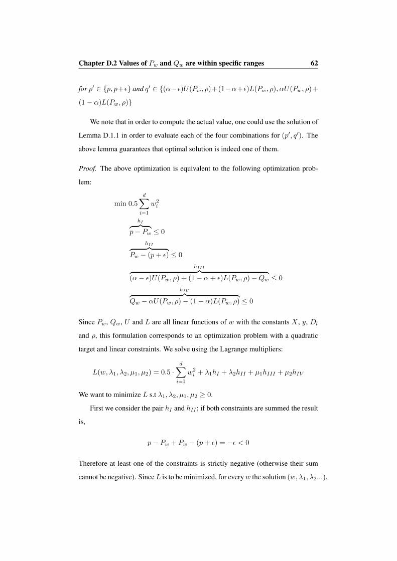
Chapter D.2 Values of Pw and Qw are within specific ranges 62
for p′ ∈ {p, p+ε} and q′ ∈ {(α−ε)U(Pw, ρ)+(1−α+ε)L(Pw, ρ), αU(Pw, ρ)+
(1− α)L(Pw, ρ)}
We note that in order to compute the actual value, one could use the solution of
Lemma D.1.1 in order to evaluate each of the four combinations for (p′, q′). The
above lemma guarantees that optimal solution is indeed one of them.
Proof. The above optimization is equivalent to the following optimization prob-
lem:
min 0.5
d∑i=1
w2i
hI︷ ︸︸ ︷p− Pw ≤ 0
hII︷ ︸︸ ︷Pw − (p+ ε) ≤ 0
hIII︷ ︸︸ ︷(α− ε)U(Pw, ρ) + (1− α+ ε)L(Pw, ρ)−Qw ≤ 0
hIV︷ ︸︸ ︷Qw − αU(Pw, ρ)− (1− α)L(Pw, ρ) ≤ 0
Since Pw, Qw, U and L are all linear functions of w with the constants X , y, Dl
and ρ, this formulation corresponds to an optimization problem with a quadratic
target and linear constraints. We solve using the Lagrange multipliers:
L(w, λ1, λ2, µ1, µ2) = 0.5 ·d∑i=1
w2i + λ1hI + λ2hII + µ1hIII + µ2hIV
We want to minimize L s.t λ1, λ2, µ1, µ2 ≥ 0.
First we consider the pair hI and hII ; if both constraints are summed the result
is,
p− Pw + Pw − (p+ ε) = −ε < 0
Therefore at least one of the constraints is strictly negative (otherwise their sum
cannot be negative). SinceL is to be minimized, for everyw the solution (w, λ1, λ2...),
Chapter D.3 Given value Pw search over Qw 63
is going to select at least one of λ1 > 0 or λ2 > 0 in order to use the negative term
and reach a smaller value of L. According to the complementary slackness this
means that either Pw = p or Pw = p+ ε (of course we cannot have both).
Next, we consider constraints hIII and hIV ; we denote with ∆ the sum be-
tween these two constraints:
∆ =(α− ε)U(Pw, ρ) + (1− α+ ε)L(Pw, ρ)−Qw +Qw − αU(Pw, ρ)− (1− α)L(Pw, ρ)
=ε (L(Pw, ρ)− U(Pw, ρ))
Since ε > 0 we only need to consider the term (L(Pw, ρ)− U(Pw, ρ)). We have
three cases: Pw = 0, Pw = 1 and 0 < Pw < 1.
For the cases Pw = 0 and Pw = 1, according to the definition of U and L
(L(0, ρ)− U(0, ρ)) = 0 or (L(1, ρ)− U(1, ρ)) = 0 correspondingly. For both
∆ = 0, and both hIII and hIV collapse to Qw = 0 or ρ. Therefore the solution is
attained either at (0, 0) for when Pw = 0 or at (1, ρ) for when Pw = 1.
Next, since for 0 < Pw < 1, L(Pw, ρ) − U(Pw, ρ) < 0 and ε > 0 therefore
∆ < 0. Similarly to the Pw constraints, according to the complementary slackness,
this means that either hIII or hIV is tight.
Therefore each minimal norm solution occurs when exactly one of hI or hII is
tight, and when one of hIII or hIV is tight. In each of those four cases, the solution
occurs in one of the corners of the cell, which in turn is the same as solving the
optimization problem for constant values of Pw and Qw for each of the corners of
the cell and taking the best solution.
D.3 Given value Pw search over Qw
This section takes a different approach then the previous ones. We search for a
feasible stochastic linear classifier given a value for only Pw. Instead of minimizing
the norm of the classifier, we search for Qw values that minimize the WGI under
the constraint that the solution is feasible.

Chapter D.3 Given value Pw search over Qw 64
The following lemma characterizes the solution when we minimize directly
WGI for a given Pw. (Note that when we fix the value of Pw the function WGI is
convex.)
Lemma D.3.1. Let ~a = D>v X and ~b = (Dv � y)>X , and assume that they are
linearly independent. Let ~b = ~b− (~a·~b)‖~a‖2~a. Then for:
w∗ = arg min WGI(p,Qw)
Pw = p
then the two solutions are,
w∗ =2p− 1
‖~a‖2~a±
√‖~a‖2 − (2p− 1)2
‖~a‖‖~b‖~b
Proof. The first observation we have is that for a fixed Pw = p, q = ρp is a
maximum for WGI, and since the second derivative of WGI is negative, we get
that WGI attains a minimal value when Qw is either maximized or minimized.
Therefore we substitute the original problem with the following two optimization
problems
Qmax = arg max Qw and Qmin = arg minQw
Pw = p Pw = p
‖w‖2 ≤ 1 ‖w‖2 ≤ 1
where the first constraint is used to fix Pw and the second constraint is used
to bound the norm of w. Now, we will translate the maximization while using the
previous expressions for ~a,~b and set p = 2p− 1.
max~b>w
~a>w − p = 0
‖w‖2 ≤ 1
We rewrite~b = α~a+ ~b as a sum of:

Chapter D.3 Given value Pw search over Qw 65
1. α · ~a which is~b’s projection over ~a.
2. ~b which is a vector that is orthogonal to a, i.e., (a · b) = 0. Since a and b are
linearly independent we have ~b 6= 0.
We write w as:
w = µ1~a+ µ2~b+ ~w
where ~w is orthogonal to ~a and ~b. The optimization becomes:
max αµ1‖~a‖2 + µ2‖~b‖2
µ1‖~a‖2 − p = 0
µ21‖~a‖2 + µ2
2‖~b‖2 + ‖ ~w‖2 ≤ 1
When we substitute µ1 = p‖~a‖2 we get:
max αp+ µ2‖~b‖2
p2
‖~a‖2+ µ2
2‖~b‖2 + ‖ ~w‖2 ≤ 1
Since αp is a constant and ‖~b‖2 is positive, the optimization is equivalent to:
max µ2
µ22‖~b‖2 + ‖ ~w‖2 ≤ 1− p2
‖~a‖2
Notice that since only µ2 is a variable that contributes to the max, we would like
to make it as large as possible under the constraint. Therefore the optimal solution
would be attained when the w = 0, and the constraint is strictly equal. Thus the
expression of µ2 would be:
µ22‖~b‖2 = 1− p2
‖~a‖2⇒ µ2 = ±
√‖~a‖2 − p2
‖~a‖‖~b‖
The maximal solution for the optimization is achieved with a positive µ2 in the
above expression:
µ2 =
√‖~a‖2 − p2
‖~a‖‖~b‖
Chapter D.4 Feasible Ranges for Pw and Qw 66
Finally the solution for w is,
w =p
‖~a‖2~a+
√‖~a‖2 − p2
‖~a‖‖~b‖~b
Notice that for the minimization problem minQw we simply select the negative
value of µ2, and get,
w =p
‖~a‖2~a−
√‖~a‖2 − p2
‖~a‖‖~b‖~b
This implies that the solution is either one of:
w∗1,2 =2p− 1
‖~a‖2~a±
√‖~a‖2 − (2p− 1)2
‖~a‖‖~b‖~b
D.4 Feasible Ranges for Pw and Qw
In all of our problems we have constraints such as Pw = p and Qw = q (or their
range variants). However we should note that not all possible values of p and q are
applicable for a given data:
Lemma D.4.1. Let ~a = D>v X and ~b = (Dv � y)>X and let w be a feasible
stochastic linear classifier. Then:
0.5− 0.5‖~a‖ ≤ Pw ≤ 0.5 + 0.5‖~a‖
0.5ρ− 0.5‖~b‖ ≤ Qw ≤ 0.5ρ+ 0.5‖~b‖
Proof. First:
− ‖~a‖‖w‖ ≤ ~a> · w ≤ ‖~a‖‖w‖ → −‖~a‖ ≤ ~a> · w ≤ ‖~a‖
− ‖~b‖‖w‖ ≤ ~b> · w ≤ ‖~b‖‖w‖ → −‖~b‖ ≤ ~b> · w ≤ ‖~b‖
where the left-hand side is a property of ·, and the right-hand is because w is feasi-
ble. Applying the above inequalities in eq 6.4: Pw = 0.5~a> · w + 0.5 and eq 6.5:
Qw = 0.5~b> · w + 0.5ρ concludes the proof.
Appendix E
Approximation Algorithms
This section details the three algorithms discussed in theorem 7.0.2:
Theorem 7.0.2. Let S be a sample, Dv be a distribution over S, and ε be an
approximation parameter. Let ~a = D>v X and~b = (Dv � y)>X . Then:
1. For the case where ~a and ~b are linearly independent, algorithms FixedPQ
and FixedPSearchQ guarantee an ε-approximation forWGI using a stochas-
tic linear classifier. Algorithm FixedPQ runs in timeO(Nd)+O(ε−2 log
(ε−1))
,
and algorithm FixedPSearchQ runs in time O(Nd) +O(dε
).
2. For the case where ~a and ~b are linearly dependent, i.e., ~b = λ~a, algorithm
DependentWGI runs in time O(Nd), and achieves the optimal result for
WGI using a stochastic linear classifier.
For each algorithm we provide pseudo code, correctness proof and a complex-
ity analysis: Algorithm FixedPQ is in Appendix E.1, Algorithm FixedPSearchQ
is in Appendix E.2 and Algorithm DependentWGI is in Appendix E.3.
As mentioned all three algorithms depend on ~a the weighted average of the
data, and ~b the weighted average of the positive class. We note here that both ~a
and ~b, along with other static related computations such as ‖~a‖, ‖~b‖ are treated as
global variables which are computed once in the beginning of each algorithm. We
67

Chapter E.1 FixedPQ Approximate minimal Gini Index in cells of Pw, Qw68
also note that the constant C = 100 used in the pseudo code corresponds to the
bound from Appendix C.
E.1 FixedPQ Approximate minimal Gini Index in cells
of Pw, Qw
In this section we describe Algorithm FixedPQ. After computing the expressions
as described earlier, we generate a list candidates that contains pairs (p, q) which
are corners of the trapezoid cells:
Initially we generate a set of equally spaces Pw values from the interval
[max (0, 0.5(1− ‖~a‖)), min (1, 0.5(1 + ‖~a‖))]. This interval is the intersection
of the domain of WGI and the feasible range of w as described in Appendix D.4.
The set of Pw values also includes the values for ρ and 1−ρ in order to ensure that
the candidates partition the domain according to the regions defined in Appendix
C.
Next, for each Pw value we define equally spaced values in ranges:
1. [max (0, p+ ρ− 1, 0.5(ρ− ‖~b‖)), min (ρp, 0.5(ρ+ ‖~b‖))]
2. [max (ρp, 0.5(ρ− ‖~b‖)),min (ρ, p, 0.5(ρ+ ‖~b‖))]
Again, these ranges take into consideration both the sub-domains of the WGI and
the feasible ranges of the stochastic linear classifier.
The equally spaced values are generated using the GetRange function, and
we always partition into Cε values in order to achieve an approximation of ε (see
correctness below). This results in O(ε−1) values of Pw, and for each of those we
have two times O(ε−1) for the Qw values below and above the line Qw = ρPw
which separates the regions. Thus, the total number of candidates is O(ε−2).
The list candidates now contains pairs of (Pw, Qw) which are sorted accord-
ing to WGI in an ascending order. For each point made of Pw and Qw values will
try to fit a stochastic linear classifier: First we use the function

Chapter E.1 FixedPQ Approximate minimal Gini Index in cells of Pw, Qw69
GetCandidateWeightsTerms to get the scalars α and β. Since we also know
‖~a‖, ‖~b‖ and (~a ·~b) we measure the feasibility of the classifier w before computing
it. Once we find a feasible classifier, we compute it explicitly and return it.
Algorithm correctness Denote w∗ the optimal feasible solution with respect to
WGI:WGIw∗ = min{w|‖w‖≤1}WGIw. LetCells be the union of non-intersecting
trapezoid cells parametrized by step size ε/C. We denote c∗ ∈ Cells the cell which
contains w∗. Denote Wc the feasible solutions proposed to cell c ∈ Cells by the
optimization in Appendix D.2 (since w∗ is feasible, we know that at least one ver-
tex is feasible). Specifically for c∗, we denote the best proposed solution as w1:
w1 = arg minw∈Wc∗
(WGI(w))
Since both w∗, w1 ∈ c∗ according to the bound we get WGIw∗ ≤ WGIw1 ≤
WGIw∗ + ε.
Next, we defineWCells as the union of the solutions from all the cells: WCells =⋃c∈CellsWc. WCells is the collection of all the classifiers that would have been
created from evaluating every point in candidates. Since Wc∗ ⊂ WCells we have
w1 ∈WCells. Let w2 be the minimal solution from all the solutions in WCells:
w2 = arg minw∈WCells
(WGIw)
In particular, WGIw∗ ≤ WGIw2 ≤ WGIw1 ≤ WGIw∗ + ε, and we notice
that w2 is actually the result returned by the algorithm. We therefore conclude that
the algorithm returns an ε approximation to the optimal WGI.
Time complexity We start by computing ρ which consists of a dot-product over
vectors of dimension N and takes time O(N). Next, we calculate ~a, ~b, by mul-
tiplying an N dimensional vector by an N × O(d) matrix, which is done in time
O(Nd). Computing the expressions that depend on ~a and~b is done once and takes
time O(d).

Chapter E.1 FixedPQ Approximate minimal Gini Index in cells of Pw, Qw70
Algorithm FixedPQ(X - dataset, Dv - data distribution, y - labels, ε -
approximation range)
1 Store globally: ρ← Dv · y,~a> ← DtvX,
~b> ← (Dv � y)>X
2 Compute once and store globally: ‖~a‖, ‖~b‖, (~a ·~b)
3 candidates← new List()
4 foreach p ∈GetRange (max (0, 0.5(1− ‖~a‖)),
min (1, 0.5(1 + ‖~a‖)), Cε )⋃{ρ, 1− ρ} do
5 foreach q ∈GetRange (max (0, p+ ρ− 1, 0.5(ρ− ‖~b‖)),
min (ρp, 0.5(ρ+ ‖~b‖)), Cε ) do
6 candidates.Insert((p, q))
end
foreach q ∈GetRange (max (ρp, 0.5(ρ− ‖~b‖)),
min (ρ, p, 0.5(ρ+ ‖~b‖)), Cε ) do
7 candidates.Insert((p, q))
end
end
8 candidates← candidates.Sort(ascending=True, by = WGI(p, q))
9 foreach p, q ∈ candidates do
10 (α, β)← GetCandidateWeightsTerms(p, q)
11 if α2 · ‖~a‖2 + 2αβ · (~a ·~b) + β2 · ‖~b‖2 ≤ 1 then
12 return(α · ~a+ β ·~b,WGI(p, q)
)end
end
13 return ”Error - Impossible”;
Procedure GetCandidateWeightsTerms(p, q)
1 p← 2p− 1 , q ← 2q − ρ
2 return(
q·(~a·~b)−p·‖~b‖2
‖~a‖2·‖~b‖2−(~a·~b)2, p·(~a·~b)−q·‖~a‖2
‖~a‖2·‖~b‖2−(~a·~b)2
)Procedure GetRange(lower, upper, steps)
1 return {p| equally spaced points in [lower,upper] with
step= upper - lowersteps }
Algorithm 2: Approximating optimal WGI with 2 ranges
Chapter E.2 FixedPSearchQ Approximate minimal Gini Index in range ofPw 71
We create a list candidates, consisting of O(ε−2) pairs (p, q) in time O(ε−2).
Next, we compute the WGI for each candidate (p, q) in O(1) time, and we sort
them using the WGI values in time O(ε−2 log (ε−2)
)= O
(ε−2 · log (ε−1)
).
Finally we try to match a classifier for each point: we iterate over (sorted)
candidates, and we call the function GetCandidateWeightsTerms which runs
in time O(1) since it is using the pre-calculated expressions. There are at most
O(ε−2)
items in the list. Therefore this step costs O(ε−2). Once a solution is
found to be feasible , only then we compute the weight vector in time O(d).
The final complexity is:
O(Nd) +O(d) +O(ε−2)
+O(ε−2 · log (ε−1)
)+O
(ε−2)
+O(d)
= O(Nd) +O(ε−2 · log (ε−1)
)
E.2 FixedPSearchQ Approximate minimal Gini Index
in range of Pw
In this section we describe Algorithm FixedPSearchQ. After computing the
expressions as described earlier, we generate a list candidates that contains values
p which are equally spaced values on the feasible range of Pw:
This set is generated from the interval [max (0, 0.5(1− ‖~a‖)),
min (1, 0.5(1 + ‖~a‖))]. This interval is the intersection of the domain of WGI and
the feasible range of w as described in Appendix D.4. The set of Pw values also
includes the values for ρ and 1 − ρ in order to ensure that the candidates partition
the domain according to the regions defined in Appendix C.
The equally spaced values are generated using theGetRange function, and we
partition into Cε values in order to achieve an approximation of ε (see correctness
below). This results in O(ε−1) values of Pw.
Next, we compute ~b which is~b minus ~a’s projection over it. This allows for the
computation of ~u and ~v. These vectors are components of the final solution.

Chapter E.2 FixedPSearchQ Approximate minimal Gini Index in range ofPw 72
Finally, for each Pw we fit two solutions which are a function of Pw, ~u and ~v.
We keep the best result w and its matching WGI g using the function
SetCandidateIfBetter, and return w and g at the end of the loop.
Algorithm correctness Given an ε parameter for the algorithm, we know that
the optimal feasible solution w∗ belongs to some range of Pw in the grid, denote
that range as C∗ = [α, β].
Denote p∗ = Pw∗ , q∗ = Qw∗ . First we note that p∗ ∈ C∗ (by definition). Next,
we consider Cq as the Q range that would have included w∗ if we were to partition
into trapezoid cells. Since w∗ is feasible, at least one of the corners of C∗ × Cq is
feasible. There is a feasible solution that we denote as wc at α or β. Without loss
of generality assume it is α. According to the bound on the WGI in Appendix C,
this candidate solution is at most ε away from w∗. Since our algorithm considers
all the possible feasible solutions for α it also considers wc and therefore the result
of the optimization problem as presented in Appendix D.3 denoted as w1 is at least
as good as wc:
WGIw1 −WGIw∗ ≤WGIwc −WGIw∗ ≤ ε
Finally, if the algorithm returns a different solutionw2 it is only becauseWGIw2 ≤
WGIw1 , and we have
WGIw∗ ≤WGIw2 ≤WGIw1 ≤WGIw∗ + ε
namely, w2 is also an ε approximation.
Time complexity We start by computing ρ which consists of a dot-product over
vectors of dimension N and takes time O(N). Next, we calculate ~a, ~b, by mul-
tiplying an N dimensional vector by an N × O(d) matrix, which is done in time
O(Nd). Computing the expressions that depend on ~a and~b is done once and takes
time O(d).

Chapter E.2 FixedPSearchQ Approximate minimal Gini Index in range ofPw 73
Algorithm FixedPSearchQ(X - dataset, Dv - data distribution, y -
labels, ε - approximation range)
1 Store globally: ρ← Dv · y,~a> ← DtvX,
~b> ← (Dv � y)>X
2 Compute once and store globally: ‖~a‖, ‖~b‖, (~a ·~b)
3 ~b← ~b− (~a·~b)‖~a‖2 · ~a
4 ~u = 1‖~a‖2 · ~a, ~v = 1
‖~a‖‖~b‖· ~b
5 w ← ⊥, g ← ⊥
6 foreach p ∈GetRange (max (0, 0.5(1− ‖~a‖)),
min (1, 0.5(1 + ‖~a‖)), Cε )⋃{ρ, 1− ρ} do
7 p← 2p− 1
8 w1 ← p · ~u+√‖~a‖2 − p2 · ~v
9 w, g ← SetCandidateIfBetter(w1,w,g,p)
10 w2 ← p · ~u−√‖~a‖2 − p2 · ~v
11 w, g ← SetCandidateIfBetter(w2,w,g,p)
end
12 if w = ⊥ then
13 return ”Error - Impossible”
end
14 return w, g
Procedure SetCandidateIfBetter(w,w,g,p)
1 q ← ~b>w+ρ2
2 if WGI(p, q) ≤ g then
3 return w,WGI(p, q)
end
4 else
5 return w, g
end
Procedure GetRange(lower, upper, steps)
1 return {p| equally spaced points in [lower,upper] with
step= upper - lowersteps }
Algorithm 3: Approximating optimal WGI with one range over Pw

Chapter E.3 DependentWGI Dependent constraints case 74
Finally the loop iterates over O(ε−1) values of p. For each such value, the
algorithm computes a weight vector and uses the method SetCandidateIfBetter
which has time complexity O(d). The total cost of all the iterations is O(dε ).
The final complexity is:
O(Nd) +O(d) +O
(d
ε
)= O(Nd) +O
(d
ε
)
E.3 DependentWGI Dependent constraints case
In this section we describe Algorithm DependentWGI. Since we have an analyt-
ical solution (Appendix C.9), we simply apply it and return its result as w and the
corresponding WGI g.
Algorithm DependentWGI(X - dataset, Dv - data distribution, y -
labels)
1 Store globally: ρ← Dv · y,~a> ← DtvX,
~b> ← (Dv � y)>X
2 Compute once and store globally: ‖~a‖
3 Get λ s.t~b = λ~a . According to our assumption, this always happens
4 w ← ~a‖~a‖
5 g ← 4(ρ− (ρ+λ‖~a‖)2
2(1+‖~a‖) −(ρ−λ‖~a‖)22(1−‖~a‖)
)6 return w, g
Algorithm 4: Approximating optimal WGI dependent case
Algorithm correctness See Appendix C.9.
Algorithm complexity We start by calculating ρ which consists of dot-product
over vectors of dimension N in time O(N). Next, we calculate ~a and ~b, by mul-
tiplying an N vector by an N × O(d) matrix in time O(Nd). Also, we calculate
‖~a‖ in time O(d). And finally, we extract λ which is O(1) without verification

Chapter E.3 DependentWGI Dependent constraints case 75
(simply, λ =~b1~a1
), or O(d) with verification (make sure that ∀i ∈ [1, d] : λ =~bi~ai
).
We compute w in time O(d) and the drop in constant time. The final complexity
is:
O(Nd) +O(d) +O(d) = O(Nd)

Appendix F
WGI not convex
In this section we are going to show that the WGI is non convex in w.
Lemma F.0.1. The function WGIw is non convex
Proof. Let x1, x2 ∈ Rd be samples s.t x1,1 = −x2,1 = 2x and ∀i ∈ [2, d] : x1,i =
x2,i (x1 and x2 are opposite in the first dimension, and the same in all other). Let
y1 = 1 be the label of x1 and let y2 = 0 be the label of x2. Also let D be the data
distribution s.t D(x1) = D(x2) = 0.5. We note that this entails that ρ = 0.5 and
that ~a1 = 0 while~b1 = x.
We define three feasible stochastic linear classifiers:
1. w0 = ~0 all zeros vector
2. w1 whose first coordinate is 1 and the rest 0: w1,1 = 1, ∀i ∈ [2, d] : w1,i = 0
3. wm whose first coordinate is 0.5 and the rest 0: w1,1 = 0.5,∀i ∈ [2, d] :
w1,i = 0.
We see that
~a>w0 = ~a>w1 = ~a>wm = 0
~b>w0 = 0, ~b>w1 = x, ~b>wm = 0.5x
76
Chapter. F: WGI not convex 77
Sice WGIw = 4(ρ− Q2
wPw− (ρ−Qw)2
1−Pw
)by equations (6.4) and (6.5) we get:
WGIw = 4
(ρ−
(~b>·w+ρ
2 )2
~a>·w+12
−(ρ− ~b>·w+ρ
2 )2
1− ~a>·w+12
)= 4
(ρ− (ρ+~b> · w)2
2(1 + ~a> · w)− (ρ−~b> · w)2
2(1− ~a> · w)
)
We substitute the values of ρ, ~a> · w and~b> · w:
WGIw0 = 4
(0.5− 0.52
2− 0.52
2
)= 1
WGIw1 = 4
(0.5− (0.5 + x)2
2− (0.5− x)2
2
)= 4
(0.25− x2
)= 1− 4x2
WGIwm = 4
(0.5− (0.5 + 0.5x)2
2− (0.5− 0.5x)2
2
)= 1− x2
Since wm = 0.5 · w0 + 0.5 · w1, in order to show non convexity we show that
WGIwm > 0.5 ·WGIw0 + 0.5 ·WGIw1 :
1− x2 > 0.5 · 1 + 0.5(1− 4x2) = 1− 2x2
which concludes the proof.

Appendix G
Approximate γ Margin With a
Stochastic Tree
In this appendix we show that the class of decision trees with stochastic linear clas-
sifiers has an efficient representation with a bounded error for a γ margin feasible
linear separator. This is show by the following theorem:
Theorem G.0.1. Let w be a γ margin feasible linear separator, then there exists a
stochastic tree T with feasible linear separators in the internal nodes such that the
error of the tree is bounded by ε and the depth of T is O(ln (ε−1)γ−2
).
Proof. Let y ∈ {0, 1} be a binary label. Let w be a linear separator such that
∀x : (2y − 1) · w · x ≥ γ. We denote Zi as a random variable such that:
Pr (Zi = 1) = 1+w·x2 and Pr (Zi = −1) = 1−w·x
2 . Let S =∑h
i=0 Zi be a
random variable which is the sum of h independent Zis. We note that E [Zi] =
1 · Pr (Zi = 1) − 1 · Pr (Zi = −1) = w · x and therefore by the expectation of a
sum E [S] =∑h
i=0E[Zi] = h(w · x).
Let x be a positive sample, meaning w · x ≥ γ. We bound the probability of
78
Chapter. G: Approximate γ Margin With a Stochastic Tree 79
the sum S to be negative by using Hoeffding’s inequality:
Pr (S ≤ 0) = Pr (S − E [S] ≤ −E [S]) = Pr (S − E [S] ≤ −h(w · x))
≤ exp−2 (h(w · x))2∑h
i=0 22= exp
−h (w · x)2
2
Since w · x ≥ γ, we get Pr (S ≤ 0) ≤ exp −hγ2
2 , and if we want to drive the
probability below ε we have:
Pr (S ≤ 0) ≤ exp−hγ2
2≤ ε→ −hγ
2
2≤ ln ε→ h ≥ 2 ln (ε−1)γ−2
Similarly, for the negative sample for Pr (S ≥ 0) ≤ ε we also require h ≥
2 ln (ε−1)γ−2.
We now describe a stochastic decision tree T : T is a full tree of depth h ≥
2 ln (ε−1)γ−2. Each internal node contains the stochastic linear separator w and
each leaf l ∈ leaves(T ) is labeled 1 if the path from root(T ) to l contains more
left turns than right and 0 otherwise.
We notice that when predicting for sample xi using T , the decision in each
internal node is modeled by Zi. A positive sample x is classified positive according
to the expectation over the leaves:
Pr (yi = 1) =∑
l∈leaves(T )
label(l) Pr (Reach(x, l))
We consider all the positive labels, since the negative labels contribute 0 to the
expectation:
Pr (yi = 1) =∑
l∈leaves(T )|label(l)=1
Pr (Reach(x, l))
By the construction of T , this probability equals the probability of reaching
leaves with more left turns than right (therefore these leaves are labeled as 1).
Namely,
Pr (yi = 1) =∑
l∈leaves(T )
label(l) Pr (Reach(x, l)) = Pr (S ≥ 0) ≥ 1− ε

Chapter. G: Approximate γ Margin With a Stochastic Tree 80
And therefore the error probability Pr (yi = 0) =≤ ε. Similarly, we can show that
the error for a negative sample is also bounded by ε. Finally this ensures that the
expected error is also smaller than ε as required.

Appendix H
Splitting criteria bounds the
classification error
In this appendix we are going to show that a permissible splitting criterion G,
upper bound twice the classification error. Reminder: a function G over [0, 1] is a
permissible splitting criterion if:
1. G is symmetric about 0.5. Thus, ∀x ∈ [0, 1] : G(x) = G(1− x).
2. G is normalized: G(0.5) = 1 and G(0) = G(1) = 0.
3. G is strictly concave.
Next, we prove the following theorem:
Theorem H.0.1. Let G be a permissible splitting criterion, then for ∀x ∈ [0, 1] :
G(x) ≥ 2 min{x, 1− x} = min{2x, 2− 2x}.
Proof. First, we consider x ∈ [0, 0.5], and we notice that min{2x, 2 − 2x} = 2x.
Next, we notice that x = (1 − 2x) · 0 + 2x · 0.5 and according to concavity of G
we derive the bound for this interval of x:
G(x) = G((1− 2x) · 0 + 2x · 0.5) ≥ (1− 2x)G(0) + 2xG(0.5) = 2x
81

Chapter. H: Splitting criteria bounds the classification error 82
Where the last transition is due to G(0.5) = 1 and G(0) = G(1) = 0.
Next, we consider x ∈ [0.5, 1], and we notice that min{2x, 2− 2x} = 2− 2x.
Again, we notice that x = (2 − 2x) · 0.5 + (1 − (2 − 2x)) · 1 and according to
concavity of G we derive the bound for this interval of x:
G(x) = G((2− 2x) · 0.5 + (1− (2− 2x)) · 1) ≥ (2− 2x)G(0.5) + (1− (2− 2x))G(1) = 2− 2x
Where the last transition is due to G(0.5) = 1 and G(0) = G(1) = 0.
The above two cases cover the interval x ∈ [0, 1] and therefore we can conclude
that ∀x ∈ [0, 1] : G(x) ≥ 2 min{x, 1− x} = min{2x, 2− 2x}.

תקציר
אנחנו בה (, boostingזו אנחנו בוחנים את בעיית למידת עצי החלטה תחת מסגרת ההגברה ) בעבודה
אשר מספקת את השערת מניחים כי המסווגים בצמתים הפנימיים של העץ שייכים למחלקת השערות (.Weak Learning Assumptionהלמידה החלשה )
ות המספקת את מחלקת ההשערות של מסווגים לינאריים סטוכסטיים, כמחלקת השערחוקרים אנחנו
לים למזעור הג'יני אינדקס אנחנו מספקים אלגוריתמים יעיעבור מחלקה זו את השערת הלמידה החלשה. (Gini Indexשהוא חסם על השגיאה א )שה ללכן, תחת הנחת הלמידה חהבעיה אינה קמורה. פילו ש
ללמידה של עצי החלטה המשתמשים במסווגים בעל חסמי שגיאהו יעיליםם מיאנחנו מספקים אלגורית .לינאריים סטוכטיים
נתונים לבסוף אנחנו בוחנים את האלגוריתם גם עבור מקרים בהם הנתונים הם סינטטיים וגם עבור
ביותר ממאפיין אחד של הנתונים בכל רגע נתון, היתרון במחלקה הנ"ל היא היכולת להתחשב אמיתיים. Support –צעת כנגד הביצועים של מפריד לינארי לכן אנחנו משווים את הביצועים של השיטה המו
Vector Machine ה המבוסס "גדי החלטות" נל לינארי וכנגד עץ החלטעם קר(decision stumps ומראים )
גבוה עם גבול החלטה מורכב המסווג המוצע עובד טוב יותר מהשניים האחרים. כי עבור נתונים ממימד

אוניברסיטת תל אביב
הפקולטה למדעים מדויקים
על שם ריימונד ובברלי סאקלר
בית הספר למדעי המחשב
לימוד עצי החלטות סטוכסטיים עם מסווגים
לינאריים
חיבור זה הוגש כחלק מהדרישות לקבלת התואר
.M.Sc –"מוסמך אוניברסיטה"
באוניברסיטת תל אביב
בית הספר למדעי המחשב
על ידי
תום יורגנסון
עבודת המחקר לתזה זו נערכה
של בהנחייתובאוניברסיטת תל אביב
ישי מנצורפרופסור
2017 יוני