linear operators and integral equations in global illumination

Linear Operators and Integral Equations

in Global Illumination �

James Arvo

Program of Computer Graphics

Cornell University

Abstract

These notes introduce the basic concepts of integral equations and their application inglobal illumination� Much of the discussion is expressed in the language of linear operatorsto simplify the notation and to emphasize the algebraic properties of the integral equations�We start by reviewing some facts about linear operators and examining some of the operatorsthat occur in global illumination� Six general methods of solving operator and integralequations are then discussed� the Neumann series� successive approximations� the Nystr�ommethod� collocation� least squares� and the Galerkin method� Finally� we look at some ofthe steps involved in applying these techniques in the context of global illumination�

� Introduction

The transfer of energy by radiation has a character fundamentally di�erent from the pro�cesses of conduction and convection� One reason for this di�erence is that the radiant energypassing through a point in space cannot be completely described by a single scalar quan�tity� even for monochromatic light� In contrast� the process of heat transfer via conductioncan be quite adequately modeled using a scalar �eld� Another di�erence is the non�localcharacter of radiant energy� light re�ected from a surface may travel undisturbed until itimpinges on a distant object� As a result of these properties� radiative transfer problemstend to be posed as integral equations� while those of conduction and convection are posedas di�erential equations �� This distinction was not always evident�

Integral equations began to appear in problems concerning the transfer of radiant energyaround the turn of the century � �� but they did not become a mainstay of radiativetransfer until much later� Up until �� much of the analysis of interre�ection was stillcarried out in a more tedious manner �� even though a signi�cant theory of integralequations was already in existence �� Buckley was one of the �rst to recast the analysisof radiative transfer problems into the modern language of integral equations �� and thislanguage has become an indispensible part of radiative transfer since then ��

�Copyright c�� by James Arvo

��

Linear Operators and Integral Equations ��

� Preliminaries

Before discussing the basics of integral equations� we need some mathematical machineryto capture the algebraic structure of functions and the operations that we perform onthem� The central theme is that of linearity� a concept that pervades the theory of integralequations and functional analysis in general� Nearly all numerical solutions ultimatelyreduce to systems of linear algebraic equations� More importantly� linearity is manifest inthe functions and equations themselves� concepts that apply in in�nite�dimensional functionspaces�

In this section we introduce a hierarchy of abstract spaces that occur repeatedly invarious guises in the study of integral equations� From least to most speci�c these spacesare the vector space� normed linear space� Banach space� and Hilbert space� The materialin this section is only a super�cial overview� For much greater depth� see any introductorytext on real analysis � ��

�� Vector Spaces and Function Spaces

A vector space� also called a linear space� is a set X along with two operations de�ned on itselements� addition and scalar multiplication� under which X is algebraically closed� That is�for any x� y � X � and � � R� the sum x� y and the scalar product �x are also elements ofX � Furthermore� the operations obey distributive laws� such as ��x� y� � �x� �y� Theseare the familiar properties of n�dimensional Euclidean space� R�� In dealing with integral ordi�erential equations� however� we encounter function spaces� that is� vector spaces whoseelements also happen to be functions� It is appropriate to refer to the elements of a functionspace either as �functions� or as �vectors�� depending on the which level of structure oneis considering�

To illustrate� we �rst consider a simple function space� the collection of all real�valuedfunctions on the interval �� which we denote by X � The elements of X form a naturalvector space if we de�ne addition and scalar multiplication of functions pointwise� That is�if f and g are two functions in X � we de�ne the sum f � g and the scalar multiple �f tobe new functions in the obvious way�

�f � g��x� � f�x� � g�x�

��f��x� � �f�x�

for each x � �� It is easy to verify that X satis�es all the properties of a vectorspace with these operations� Precisely the same constructions apply to functions of severalvariables� such as radiance functions� We will encounter vector spaces at three dinstinctlevels� Euclidian n�dimensional space� function spaces� and Banach spaces of operators�

The dimension of a vector space is the maximal number of linearly independent ele�ments� It is easy to see that the space X above is in�nite dimensional� since the Fourierbasis functions sin�n�x�� for n � � �� are all linearly independent on �� In most prob�lems involving function approximation the desired function is a member of some in�nite�dimensional space� To be representable on a computer� however� the approximation mustlive in a space of only �nite dimension� The main task of numerical methods is to makethe transition in such a way that we reliably capture all relevant features of the originalfunction�


�� Normed Linear Spaces and Banach Spaces

In addition to the purely algebraic structure of a vector space� we require some notion ofthe size of the individual elements in order to speak of convergence and to quantify error�To do this� we supply the vector space X with a real�valued function

jj�jj � X � ��

called a norm� A norm is intended to capture the essence of size in an abstract space� Forany x� y � X and � � R� a norm must satisy

� jjxjj � � for x ��

�� jj�xjj � j�j jjxjj

� jjx� yjj � jjxjj� jjyjj�

where the third property is known as the triangle inequality� A vector space equipped witha norm is called a normed linear space� In general there are many possible norms that canbe de�ned on a given vector space� For Rn� two common norms are the Euclidean norm

jjxjj��

�nXi��

x�i

��

and the uniform or in�nity norm

jjxjj�� maxfjx�j � � � � � jxnjg�

Given a norm� we can measure the �distance� between two vectors by de�ning a functionknown as a metric�

d�x� y� � jjx� yjj �

Thus� a norm also carries with it an abstract notion of distance� In the context of functionspaces� the only norms we will need to consider are the so called p�norms� de�ned by

jjf jjp �

�Zjf�x�j

pdx

��p� � �

As it stands� the above is merely a formal de�nition because the integral may fail to existfor a given function� We de�ne the set Lp�� to be the set of functions de�ned on theinterval �� for which the integral makes sense and is �nite� Since linear combinations ofelements in Lp retain these properties� it is a normed linear space with the norm jj�jjp� Weshall make use of the spaces L� and L��

Another property that a normed linear space may possess is that of �topological� closure�We say a space is closed if convergent sequences always converge to something in the space�That is� if the sequence x�� x�� is such that

limn��

jjx� xnjj � ��

then x � X � Closure is always relative to some larger space� but the analogous property ofcompleteness is intrinsic to a space� In e�ect� completeness guarantees that there is alwaysan x in the space to converge to� A complete normed linear space is called a Banach space�Function spaces may be complete with respect to one norm but not another� a complicationthat does not arise in �nite dimensional spaces�


�� Hilbert Space

The next rung up the ladder of structure involves adding the concept of an inner productto the space� An inner product on a �real� vector space X is a real�valued function de�nedon X �X � denoted h� j �i� with the following properties�

� hx j xi �

�� hx j yi � hy j xi

� h�x � �y j zi � � hx j zi� � hy j zi�

The third property says that the inner product is linear in the �rst argument� by the secondproperty linearity holds for the second argument as well� making the inner product bilinear�Given an inner product we can always de�ne a norm by

jjxjj �qhx j xi� ��

so a space with an inner product is automatically a normed space� However� not all normscan be de�ned by means of an inner product� and those that can be have very specialproperties� A Banach space whose norm comes from an inner product is called a Hilbert

space� Euclidian n�space is a Hilbert space with the inner product corresponding to thestandard dot product� The space L�� is a Hilbert space of functions� and the innerproduct corresponding to its norm is

hf j gi �

�Zf�x� g�x� dx

��

But the �norm and ��norm do not have corresponding inner products� so L� and L� arenot Hilbert spaces� Hilbert spaces have a very geometrical �avor because the inner productgives rise to the notion of orthogonality� We say that two vectors x and y are orthogonal�and write x y� if

hx j yi � ��

Similarly� a vector x is said to be orthogonal to a set S � X � denoted x S� if x y forall y � S� One of the most important properties of Hilbert spaces is that its elements canbe approximated by projecting them onto some convenient subspace� typically one of �nitedimension ��

� Linear Operators

A mapping T from a vector space X to a vector space Y is said to be linear if it satis�es

T��x� �y� � �T�x� � �T�y� ��

for any x � X � y � Y � and any scalars � and �� In analogy with matrix notation� it istraditional to write Tx instead of T�x� if T is linear� Furthermore� if the domain of T is afunction space� we call it a linear operator� The most important linear operator for us will


be the integral operator� Let k � �� R be a continuous function on the unit square andconsider the operator K de�ned by

K �

Z �

�

k�� y� � dy� ��

where the brackets are meant to accomodate a function of y� A more explicit way to writethis is to show its action on a function f �

�Kf��x� �

Z �

�

k�x� y� f�y� dy� ��

The above form of integral operator called a kernel operator� and k is called the kernel� Thekernel k is essentially an extension of the concept of a matrix to an in�nite dimensionalfunction space �� It is easy to verify that K is a linear operator over an appropriatedomain X � such as L�� Indeed� for any f� g � L�� we have

K�f � g��x� �

Z �

�

k�x� y� f � g��y� dy

�

Z �

�

k�x� y� f�y�� g�y�� dy

�Z �

�

k�x� y� f�y� dy�Z �

�

k�x� y� g�y�dy

� �Kf��x� � �Kg��x��

Since this holds for all x � �� by de�nition the functions themselves are equal�

K�f � g� � Kf �Kg� ��

Similarly� it can be shown thatK��f� � �Kf � Therefore� K satis�es equation �� showingthatK is a linear operator on L�� Other frequently occurring linear operators includethe multiplication operator� de�ned by

�Mgf��x� � g�x� f�x��

where g is any bounded function in X � and the real�valued evaluation operator� de�ned by

Exf � f�x��

where x is any point in the domain� Finally� if the space X is a Hilbert space� such asL�� we can de�ne a projection operator by

Pnx �nXi��

yi hx j yii � ��

where y�� yn are arbitrary elements of X � It is straightforward to verify the linearity ofeach of these operators�


�� Operator Norms

Let X and Y be any two normed linear spaces and consider the collection of all linearoperators A � X � Y � This collection is itself a vector space because sums and scalarmultiples of linear operators are again linear operators� We can turn this vector space ofoperators into a normed linear space by de�ning the norm

jjKjj � supfjjKf jjY � jjf jjX � g� � �

which is called the operator norm� Here the subscripts indicate which space each norm isde�ned in� as there are three di�erent norms involved in the above de�nition� An equivalentde�nition that follows from the one above is

jjKjj � supf ��

jjKf jjYjjf jjX

� � ��

Henceforth we shall drop the subsripts on operator norms since the space it applies to isalways clear from context� As an immediate consequence of the above de�nition� we havethe inequality

jjKf jj � jjKjj jjf jj � � ��

A bounded linear operator is one with �nite norm� The set of all bounded linear operatorsfrom X to Y is a normed linear space with the operator norm� Furthermore� this normedlinear space is always complete� making it a Banach space� we denote it by B�X� Y �� orsimply B�X� if X � Y �

The space B�X� has some additional algebraic structure that is not inherent in a normedlinear space� This is because linear operators from a space into itself can be composedwith one another� providing a form of multiplication� Operator norms are compatible withoperator multiplication in that

jjABjj � jjAjj jjBjj � ��

�� Transfer Equations

The equations governing the transport of radiant energy have some intrinsic properties thatbecome more apparent when written in terms of linear operators� Operator notation has theadvantage of supressing the cumbersome notation of integral operators while emphasizingthe role of integrals as transformations� Consider the stationary equation of transfer givenby

� � rL�r� �� r�L�r� �� r� ��

ZS�k�r�� L�r� �� d��

for r � R� and � � S�� where S� is the the unit sphere in R�� This equation is frequentlywritten more succinctly using operator notation�

� � r� ��r��K�L�r� �� r� ��

where K is de�ned by

�Kf��r� ��

ZS�k�r�� f�r� �� d��


All three of the operators on the left�hand side of equation � �� are linear� Note that ��r�corresponds to Mg of equation � �� with g�r� �� r�� Although K is not in the formof equation �� it is easy to see its relation to a standard kernel operator by de�ning thefamily of operators

�Krh��x� �

ZS�kr�x�y� h�y� dy ��

where r � R�� h is a function of a single vector x� and kr�x�y� � k�r�x � y�� Then Kr is akernel operator for each r � R�� and the action of K can be expressed as

�Kf��r� �� Krf�r� ��

Here f�r� �� is a form of evaluation operator� and the Kr act as an operator analogue of themultiplication operator� with the Kr chosen on the basis of the �rst argument� Breakingan operator into components is often a means of estimating its norm using equation � ��Finally� we can write equation � �� as

GL � ��

where G is a linear operator� This reveals at a glance the superposition principle� namely�that solutions corresponding to di�erent sources can be superposed� If GL� � �� andGL� � �� then

G�L� � L��

For an inexhaustible source of information on operator norms and function spaces� see theclassic three�volume magnum opus by Dunford and Schwartz ��

� Fredholm Integral Equations

To introduce the notion of an integral equation� we begin by considering the followingproblem� given a function g and a kernel k� �nd a function f that satis�es

f�x� �Z �

�

k�x� y� g�y�dy� ��

or� in operator notation�

f � Kg ��

where K is the kernel operator corresponding to k� Solving this problem numerically is verystraightforward� it is nothing more than a problem of integration for each x� Assuming wecan evaluate the functions k and g anywhere we choose� it can be solved approximately usinga variety of numerical quadrature techniques� For instance� we could use any quadraturerule of the form

f�x� �nXi��

wi k�x� yi� g�yi� ��


for a sequence � y� y� � � � yn � � and weights wi� The problem has a radicallydi�erent character� however� if we exchange the roles of the functions f and g� That is�given a function g and a kernel k� �nd the function f that satis�es

g�x� �Z �

�

k�x� y� f�y� dy� ��

Equation �� is known as a Fredholm integral equation of the �rst kind� It is equivalent toinverting a kernel operator�

f � K��g� ��

when the inverse exists� Note� however� that if there are multiple solutions to equation ��then the inverseK does not exist� Now consider a problem of a slightly di�erent form� givena function g and a kernel k� �nd a function f that satis�es

f�x� � g�x� �

Z �

�

k�x� y� f�y� dy� ��

Equation �� is known as a Fredholm integral equation of the second kind� The �nd kindintegral equations at �rst appear to be more complex because the unknown function f

appears in two places� But by representing the f outside the integral as If � where I is theidentity operator� we can again write f as a single operator times g�

f � �I�K��g� ��

The two varieties of Fredholm integral equations actually have quite di�erent properties�For instance� if k and g are step functions� then the solution f to equation �� must alsobe a step function �� yet we can say nothing about the form of f in equation �� Thisfact would seem to indicate that �nd kind equations are in some sense nicer to work withthan st kind equations� This is indeed the case� Fortunately� the integral equations weencounter in radiative transfer are of the �nd kind�

� Approximate Solutions to Integral Equations

Very few integral equations that arise in practice admit closed�form solutions� especiallyin global illumination� where the complex geometry of environments makes closed�formsolutions hopeless� Therefore we need to rely upon numerical methods� A large assortmentof numerical techniques exist for solving integral equations �� and we shall only touch on afew of them� To illustrate the principles� assume K � X�X is a bounded linear operator�where X is a space of functions de�ned over a domain D� We assume that X � L��D�unless we require the structure of a Hilbert space� as in the �nite basis methods discussedbelow� We wish to approximate the solution to

f � g �Kf� � �

Of course� equation � � is equivalent to Af � g� where A � I � K� Although much ofwhat follows applies to any non�singular A� including equations of the st kind� we willfocus exclusively on the �nd kind equations�


�� Neumann Series

The Neumann series � � method is based on the operator analogue of the familiar geometricseries

� x� � x � x� � � � � for jxj � ��

When jxj is su�ciently small� � x cannot be zero� so it must have an inverse� The sameholds for linear operators� where size is de�ned by the operator norm� Thus� jjKjj implies that the operator I�K has an inverse� which is given by the Neumann series

�I�K��

��Xj��

Kj ��

� I�K�K� � � � � � ��

Now� suppose that the operator K of equation � � has norm less than one� and de�ne

M � �I�K��

Then the operator equation � � has the solution

f �Mg � g �Kg �K�g � � � � � ��

We now investigate approximations based on this in�nite series� Let Mn be the operatorobtained by truncating the series after n terms�

Mn �nXj��

Kj � ��

Then Mn will be an approximation of the exact operator M� The error incurred by ter�minating the series can be estimated by making use of the various properties of operatornorms� Thus

jjM�Mnjj �

��

�Xj�n��

Kj

��

�Xj�n��

��Kj�� X

j�n��

jjKjjj� ��

where the �rst inequality follows from the triangle inequality� and the second inequalityfollows from equation � �� Extension to an in�nite series follows from the continuity ofnorms� The �nal expression in equation �� is a geometric series of real numbers� whichhas a simple formula� Thus� we have

jjM�Mnjj �jjKjj

n��

� jjKjj� ��

Equation �� indicates how close Mn is to the exact operator in terms of the operatornorm� but as yet we�ve said nothing about how well we can approximate the function f byfunctions of the form

fn �Mng� ��


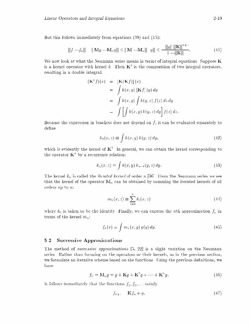
But this follows immediately from equations �� and � ��

jjf � fnjj � jjMg �Mngjj � jjM�Mnjj jjgjj �jjgjj jjKjj

n��

� jjKjj� ��

We now look at what the Neumann series means in terms of integral equations� Suppose Kis a kernel operator with kernel k� Then K� is the composition of two integral operators�resulting in a double integral�

�K�f��x� � K�Kf�� x�

�Zk�x� y� Kf � �y� dy

�

Zk�x� y�

Zk�y� z� f�z� dzdy

�Z �Z

k�x� y� k�y� z� dy

�f�z� dz�

Because the expression in brackets does not depend on f � it can be evaluated separately tode�ne

k��x� z� �

Zk�x� y� k�y� z�dy� ��

which is evidently the kernel of K�� In general� we can obtain the kernel corresponding tothe operator Kn by a recurrence relation�

kn�x� z� �Zk�x� y� kn��y� z� dy� ��

The kernel kn is called the iterated kernel of order n �� From the Neumann series we seethat the kernel of the operator Mn can be obtained by summing the iterated kernels of allorders up to n�

mn�x� z� �nXi��

ki�x� z� ��

where k� is taken to be the identity� Finally� we can express the nth approximation fn interms of the kernel mn�

fn�x� �

Zmn�x� y� g�y�dy� ��

�� Successive Approximations

The method of successive approximations �� is a slight variation on the Neumannseries� Rather than focusing on the operators or their kernels� as in the previous section�we formulate an iterative scheme based on the functions� Using the previous de�nitions� wehave

fn �Mng � g �Kg �K�g � � � ��K

ng� ��

It follows immediately that the functions f�� f�� satisfy

fn�� Kfn � g� ��


In terms of the corresponding integral equation� we have the simple recurrence relation�

f� � g

fn��x� � g�x� �Zk�x� y� fn�y� dy�

Because equation �� holds for fn� we are guaranteed that fn converges to f as n��whenever jjKjj �

�� The Nystr�om Method

The Nystr�om method� also known as the quadrature method �� is one of the moststraightforward numerical methods for integral equations� It directly exploits the similaritybetween the kernel of an integral operator and its �nite�dimensional analog� the matrix�The idea is to estimate the action of the integral operator by a quadrature rule� producinga system of linear algebraic equations� To do this� we select n points x�� xn in D atwhich to approximate the values of f � That is� we wish to �nd values y�� yn such that

yj � f�xj�

for j � � � � � � n� We use the fact that for each x� the value of f�x� can be approximated bya quadrature rule based on the values of f at the points x�� xn�

f�x� � g�x� �nXi��

wi�x� k�x� xi� f�xi��

where k is the kernel associated withK� The weights w��x�� wn�x� de�ne the quadraturerule and may vary with the choice of x� We apply this strategy at each of the n pointsx�� xn to de�ne n equations in the unknowns y�� yn�

yj � g�xj� �nXi��

wi�xj� k�xj� xi� yi�

Writing this in matrix form� �nding the y�s reduces to computing��y�y��yn

� �

�� w��k�� w��k�� wn�k�n�w��k�� w��k�� wn�k�n

��

� � ��

�w�nkn� �w�nkn� � � � � wnnknn

��

g�x��g�x��

g�xn�

� � ��

where wij � wi�xj� and kij � k�xi� xj�� Note that we need only evaluate the functionsg and k at a �nite number of points to set up the matrix equation above� This propertymakes the Nystr�om method extremely versatile�

�� Finite Basis Methods

The common thread running through the following three methods is the concept of approx�imating a function space with a �nite�dimensional subspace� In practice� the subspace willbe the span of some �nite collection of basis functions chosen for their convenient proper�ties� hence the name �nite basis methods �� To describe the methods in abstract terms�


however� we needn�t know anything concrete about the subspace� we are simply given ann�dimensional subspace of X � denoted Xn� with basis functions fu�� ung� That is� theui are functions in X such that

Xn � Spanfu�� ung�

Our goal is to �nd fn � Xn which is in some sense a good approximation of f � which reducesto �nding n scalar values �� n such that

fn �nXi��

�iui� ��

This is always possible for fn � Xn since u�� un is a basis� For this reason� �nite basismethods are also known as methods of undetermined coe�cents�

A fundamental operation that appears repeatedly in all of the �nite basis methods isthe application of the operator I �K to some function in the space X � In the interest ofbrevity� we introduce the notation

bh � �I�K�h

for any function h � X � Thus� the notation bh�x� is to be interpreted as �I�K�h��x�� Withthe new notation� the exact solution f of equation � � satis�es

bf � g�

Of course� �nding such an f is impossible in practice� so we settle for an approximationfn � Xn� The central property that distinguishes the following three methods is theircriteria for selecting fn from a given space of functions Xn�

�� Collocation

In the collocation method� the approximate function fn is chosen from the n�dimensionalsubspace Xn by requiring the transformed function bfn to attain the desired value at a �nite

number of points �� That is� we select n points x�� xn from D� and require that bfnsatisfy

bfn�xj� � g�xj� ��

for j � � � � � � n� From equation �� and the de�nition of bfn we have

bfn � �I�K�nXi��

�iui

�nXi��

�i�I�K�ui

�nXi��

�ibui� ��

The requirement that bfn agree with g at n points results in n linear equations in �i�

nXi��

�ibui�xj� � g�xj� ��


for j � � � � � � n� In matrix form� the solution for � is�� n

� �

�� bu��x�� bun�x��

� � ��bu��xn� � � � bun�xn�

�� g�x��

��g�xn�

� � ��

Note that collocation does not enforce equality of fn and f at the points x�� xn� Becauseequation �� constrains only bfn� we can expect that fn�xj� �� f�xj� in general� However�for suitably placed collocation points� the approximation will converge to the exact valuesas n��

�� The Least Squares Method

The least squares method �� is a very straightforward application of Hilbert spacemethods to integral equations� Again� the goal is to �nd fn � Xn that in some senseapproximates f � only the criterion now is to choose fn in the sense of least squares mini�mization� we seek fn � Xn such that �� bfn � g

��

is minimized� That is� the approximation fn is selected so that�� bfn � g��

� jj�I�K�h� gjj�

for all h � Xn� This is the best we can do within the subspace Xn� For the ��normto even make sense� we assume here that X � L��D�� which also possesses the Hilbertspace structure that we need to perform the least squares approximation� If the domainD is bounded �more precisely� of �nite measure�� then L��D� � L��D� �� which meansthat there are �fewer� functions to choose from in least squares than in methods such ascollocation� For the most part this causes no practical di�culties other than disallowingfunctions with rather severe singularities� To make use of the Hilbert space structure� wede�ne

Yn � f bfn � fn � Xng

and note that Yn is a subspace of X � the image of one subspace under a linear operator isanother subspace� Now we can frame the original problem in geometrical terms� the taskof �nding the function bfn � Yn that is is closest to g corresponds to projecting the functiong onto the subspace Yn� Equivalently� if bfn is the projection of g onto Yn� then the residualerror incurred by bfn will be orthogonal to the subspace Yn�

� bfn � g� Yn� ��

See Figure � �� We now proceed to �nd the fn � Xn corresponding to bfn� To do this�we apply the usual tricks� expanding functions in terms of basis functions and exploitinglinearity of operators and bilinearity of inner products� First� observe that since u�� unis a basis of Xn� we automatically have that

Yn � Spanfbu�� bung�


g - fn

g

Yn fnO

Figure � The least squares approach �nds the projection of g onto Yn� which minimizes the

��norm of the error�

Therefore� the requirement that bfn � g be orthogonal to Yn is equivalent toD bfn � g�� buiE � � ��

for i � � � � � � n� Using the bilinearity of the inner product� we can write this as

hg j buii � D bfn �� buiE ��

for i � � � � � � n� But� by equation �� we have

bfn �nXi��

�ibui�Substituting this expansion for bfn into equation �� we have

hg j buji �

�nXi��

�ibui�� buj

�

�nXi��

�i h bui j buji � ��

which is again a set of linear algebraic equations in �� In matrix form� the formal solutionfor � is ��

��n

� �

�� h bu� j bu�i � � � h bun j bu�i��

� � ��

h bu� j buni � � � h bun j buni�� hg j bu�i

��hg j buni

� � ��

Equation �� consists of the familiar normal equations of the least squares method� Thematrix of inner products is a Gram matrix� which is nonsingular provided that the functionsbu�� bun are linearly independent ��

�� The Galerkin Method

The Galerkin method also requires the structure of a Hilbert space� in fact� its form isalmost identical to the least squares method� The di�erence� again� is in the criterion forpicking the approximation bfn� In the least squares method� we required the residual bfn � g


to be orthogonal to all of Yn� as stated by equation �� In general� the bigger the space Ynis� the smaller the residual is forced to be� But will another space do the job� The answeris yes� The key observation of the Galerkin method is that we can use the space Xn itselfinstead of its image� Yn� Thus� we replace equation �� with the requirement that

� bfn � g� Xn� ��

If Xn is similar to Yn� meaning that I�K maps much of Xn into itself� then the Galerkinmethod will produce an answer that is close to optimal in the least squares sense� SeeFigure �� To see the Galerkin method another way� let Pn be the projection operatoronto Xn� Then solving equation �� is equivalent to �nding fn � Xn such that

Pn� bfn � g� � ��

which is equivalent to solving

�I� PnK�fn � Png�

since Pnfn � fn� So the Galerkin method seeks a solution that is exact once K and g

have had their ranges collapsed onto the n�dimensional space Xn �� In analogy withequation �� equation �� is equivalent toD bfn � g

�� uiE � � ��

for i � � � � � � n� Equivalently�

hg j uii �D bfn �� uiE

which is analogous to equation �� Following the very same steps as in the least squaresmethod� we arrive at the expression

hg j uji �nXi��

�i h bui j ujiwhich corresponds to equation �� Finally� the matrix equation for � arising from theGalerkin method is��

��n

� �

�� h bu� j u�i � � � h bun j u�i��

� � ��

h bu� j uni � � � h bun j uni�� hg j u�i

��hg j uni

� � ��

The Galerkin method is also know as the method of moments because equation �� requiresthat the �rst n generalized moments of the function bfn � g be zero ��

� Applications to Global Illumination

In this section we will look at how the principles discussed above have been employed inglobal illumination� and radiative transfer in general� We will focus on the problem of directexchange of radiant energy between surfaces� that is� radiative transfer in the absence of


g - fn

g

YnXn

fnO

Figure �� In the Galerkin method� the residual error g� bfn is forced to be orthogonal to the

space of basis functions Xn rather than its image Yn�

a participating medium� The governing equation in this restricted case is a functionalequation of the form

L � ��KL� ��

where L is the radiance function W m�� sr�� de�ned over surfaces and directions� � is theemitted radiance of the surfaces� and K is a linear operator� Both � and K are implicitlyassumed to be functions of wavelength� Let M represent the surfaces in R�� which weassume to form an enclosure� Then L and � are functions of the form f � H��R� whereH� is the set of rays leaving the surface M � We will represent a single ray by �s� �� wheres �M � and � is a unit vector� The linear operator K has the form

�Kf��s� �� Z�s�� cos �i f�s

�� d��

for �s� �� H� � where the integration is over the incident hemisphere at each point s �M �and �s� �� is the bidirectional re�ectance function at that point� Here the angle �i is theangle of incidence of �� and the point s� is given by the ray shooting function ��

s� � ��s��

which is the point of intersection with M of a ray emanating from s in the direction ��Energy conservation implies that the operator K is bounded� with jjKjj �

Polyak used iterated kernels as well as the method of successive approximations to an�alyze equation �� and some of its simpler forms �� Kajiya used the Neumann seriesof an operator equation similar to equation �� to illustrate the e�ects of various approxi�mations used in computer graphics �� The successive kernels� or terms of the expansion�correspond to rays that have undergone increasing numbers of re�ections� This very natu�ral physical interpretation is often referred to as successive orders of scattering in radiativetransfer literature ��

The method of discrete ordinates used in radiative heat ransfer � �� atmosphericscattering �� and neutron transport �� works by applying quadrature rules to discretelysampled positions and directions� Thus� it is essentially an application of the Nystr�om


method� A major advantage of the Nystom method is that it can easily accomodate dif�ferential operators by means of �nite di�erence approximations� This makes it readilyapplicable to problems involving participating media�

The �nite basis approaches have been the most prevelant in global illumination� partic�ularly collocation �� The most important de�ning feature of any �nite basis method isthe choice of basis functions u�� un � X � and in the case of collocation� the collocationpoints x�� xn � D� Given the basis functions� the task is to compute the coe�cients�� n� This ultimately reduces to solving a system of n linear equations� for whichthere are numerous robust numerical methods �� By far the most challenging part ofsolving for the ��s is forming the matrix� This is also true of methods in which there is noexplicit matrix� as in progressive radiosity� where the matrix elements are computed onlyas they are needed ��

Consequently� the choice of basis functions and collocation points is heavily in�uencedby the computational requirements of forming the matrix equation� We now look at whatis involved in setting up these equations for each of the �nite basis methods� beginning withcollocation� For the collocation method� the ij�th matrix element is de�ned by

bui�xj� � ui�xj�� Kui��xj��

so there are three operations that need to be performed in order to set up the right�handside of equation ��

� Evaluate g�xj� for all j

�� Evaluate ui�xj� for all i and j

� Evaluate �Kui��xj� for all i and j

The most di�cult of these is the last� as it involves the transformation of a function by theoperator K� To apply to equation �� the collocation points must consist of a sequence ofrays� �s�� sn� �n�� and the basis functions must be of the form ui � H��R� Then

�Kui��sj� �j� �

Z�sj ��

��j� cos �i ui�s�j � �

�� d��

is the radiance at point sj in the direction �j due to a single re�ection of the radiantenergy emitted according to the basis function ui� For most basis functions� equation ��is extremely di�cult to evaluate� However� let us simplify the problem by restricting thesurfaces to be pure di�use re�ectors� which removes the angular dependence from all theradiance functions� To further simplify� we can break M into n disjoint patches� P�� Pn�letting the basis functions u�� un be given by

ui�s� �

if s � Pi� otherwise�

��

Then the �nite�dimensional subspace Xn spanned by u�� un consists of step functions�that is� functions that are constant over the patches P�� Pn� Finally� let the collocationpoints s�� sn be the midpoints of the patches� In this greatly simpli�ed case� we have

ui�sj� � ij � ��


because only the point si is within the support of basis function ui� Changing the integrationover solid angle to a surface integral� we have

�Kui��sj� � �sj�

ZPi

cos �� cos ��r�

vis�sj � s� ds� ��

which results in the well�known radiosity formulation for di�use environments� The cor�responding problem is much harder for the least squares method� where the ij�th matrixelement is de�ned by

h bui j buji � hui j uji � hKui j uji � hui j Kuji� hKui j Kuji � ��

Here� even the di�use piecewise�constant assumptions do little to reduce the di�culty ofcomputing the matrix in equation �� This is because the �nal inner product in equa�tion �� involves two functions that are potentially de�ned over the entire environment� the�nite support of the basis functions disappears when K is applied� Consequently� the leastsquares method has not yet found application in solving the integral equations of globalillumination� The situation is quite di�erent for the Galerkin method� however� where theij�th matrix element is given by

h bui j uji � hui j uji � hKui j uji � ��

This expression is still complex� but managable in the di�use case� Zatz took this approach�choosing polynomial basis functions de�ned over individual patches �� The resultingexpressions for hKui j uji require quadruple integrals� yet their support is limited to thepair of patches involved� making the computation of the inner products feasible�

Heckbert attacked the di�use case using the �nite element method� which is a specialcase of the Galerkin method �� in which the basis functions have very local support� Theadvantage of �nite elements in global illumination is that the element boundaries can beused to more accurately model discontinuities of various orders in the radiance functions�Thus� the emphasis here is on increased accuracy as opposed to producing a sparse matrix�which is one of the traditional bene�ts of the �nite element method ��

References

�� Kendall E� Atkinson� A Survey of Numerical Methods for the Solution of Fredholm Integral

Equations of the Second Kind� Society for Industrial and Applied Mathematics� Philadelphia��

�� H� Bateman� Report on the history and present state of the theory of integral equations� Reportof the ��th Meeting of the British Association for the Advancement of Science� pages �� She�eld� August � � September ��

�� Maxime B�ocher� An Introduction to the Study of Integral Equations� Cambridge UniversityPress� Cambridge� ��

�� H� Buckley� On the radiation from the inside of a circular cylinder� Philosophical Magazine�� October ��

�� Hans B�uckner� A special method of successive approximations for Fredholm integral equations�Duke Mathematical Journal� ��


�� I� W� Busbridge� The Mathematics of Radiative Transfer� Cambridge University Press� Bristol��

�� B� G� Carlson and K� D� Lathrop� Transport theory � the method of discrete ordinates� InH� Greenspan� C� N� Kelber� and D� Okrent� editors� Computing Methods in Reactor Physics�pages �� Gordon and Breach� New York� ��

�� Michael F� Cohen� Shenchang Eric Chen� John R�Wallace� and Donald P� Greenberg� A progres�sive re�nement approach to fast radiosity image generation� Computer Graphics� ��August ��

�� L� M� Delves and J� L� Mohamed� Computational Methods for Integral Equations� CambridgeUniversity Press� New York� ��

�� Nelson Dunford and Jacob T� Schwartz� Linear Operators� John Wiley � Sons� New York��

�� W� A� Fiveland� Discrete�ordinates solutions of the radiative transport equation for rectangularenclosures� ASME Journal of Heat Transfer� � ��

�� Gene H� Golub and Charles F� Van Loan� Matrix Computations� Johns Hopkins� Baltimore�MD� ��

�� P� R� Halmos and V� S� Sunder� Bounded Integral Operators on L� Spaces� Springer�Verlag�

New York� ��

�� Paul S� Heckbert� Simulating Global Illumination Using Adaptive Meshing� PhD thesis� Uni�versity of California� Berkeley� June ��

�� Francis B� Hildebrand� Methods of Applied Mathematics� Prentice�Hall� New York� ��

�� Eberhard Hopf� Mathematical Problems of Radiative Equilibrium� Cambridge University Press�New York� ��

�� Yasuhiko Ikebe� The Galerkin method for the numerical solution of Fredholm integral equationsof the second kind� SIAM Review� �� July ��

�� W� H� Jackson� The solution of an integral equation occuring in the theory of radiation� Bulletinof the American Mathematical Society� �� June ��

�� James T� Kajiya� The rendering equation� Computer Graphics� � �� August ��

�� L� V� Kantorovich and V� I� Krylov� Approximate Methods of Higher Analysis� IntersciencePublishers� New York� �� Translated by C� D� Benster�

�� Tosio Kato� Perturbation Theory for Linear Operators� Springer�Verlag� New York� ��

�� Rainer Kress� Linear Integral Equations� Springer�Verlag� New York� ��

�� K� D� Lathrop� Use of discrete�ordinate methods for solution of photon transport problems�Nuclear Science and Engineering� �� April ��

�� Jacqueline Lenoble� editor� Radiative Transfer in Scattering and Absorbing Atmospheres� Stan�

dard Computational Procedures� Studies in Geophysical Optics and Remote Sensing� A� Deepak�Hampton� Virginia� ��

�� David G� Luenberger� Optimization by Vector Space Methods� John Wiley � Sons� New York��

�� Parry Moon� On interre�ections� Journal of the Optical Society of America� ��

�� Ramon E� Moore� Computational Functional Analysis� Academic Press� New York� ��


�� G� L� Polyak� Radiative transfer between surfaces of arbitrary spatial distribution of re�ection�In Convective and Radiative Heat Transfer� Publishing House of the Academy of Sciences ofthe USSR� Moscow� ��

�� David Porter and David S� G� Stirling� Integral equations� A practical treatment� from spectral

theory to applications� Cambridge University Press� New York� ��

� � H� L� Royden� Real Analysis� The Macmillan Company� New York� second edition� ��

�� Walter Rudin� Principles of Mathematical Analysis� McGraw�Hill� New York� second edition��

�� Walter Rudin� Real and Complex Analysis� McGraw�Hill� New York� second edition� ��

�� Arthur Schuster� The in�uence of radiation on the transmission of heat� Philosophical Magazine�� February ��

�� E� M� Sparrow� Application of variational methods to radiative heat�transfer calculations�ASME Journal of Heat Transfer� �� November ��

�� Gilbert Strang and George J� Fix� An Analysis of the Finite Element Method� Prentice�Hall�Englewood Cli�s� New Jersey� ��

�� F� G� Tricomi� Integral Equations� Dover Publications� New York� ��

�� Ziro Yamauti� The light �ux distribution of a system of interre�ecting surfaces� Journal of theOptical Society of America� ��

�� W� W� Yuen and C� L� Tien� A successive approximation approach to problems in radiativetransfer with a di�erential approximation� ASME Journal of Heat Transfer� � ��February ��

�� Harold Zatz� Galerkin radiosity� A higher order solution method for global illumination� InComputer Graphics Proceedings� Annual Conference Series� ACM SIGGRAPH� pages ��


1:

Two ways to get updated notes:

2:

Anonymous ftp:

Electronic [email protected]

ray.graphics.cornell.edudirectory pub/arvo

Linear Operators and Integral Equations

Linear operators are to functions asmatrices are to vectors

Radiative transfer is most readilyexpressed using integral equations

Integral equations can be studied as operator equations

f(x) = k(x,y) g(y) dy

Given functions k and g, find f such that

Σf(x) ≅i=1

n

Solve with quadrature for each x:

w i k(x,y i) g(y i)

An Integration Problem Fredholm Integral Equation (First Kind)


No longer a simple problem of numerical quadrature. In operator notation

g(x) = k(x,y) f(y) dy

g = K f

Fredholm Integral Equation

The corresponding second-kind operatorequation is

(Second Kind)


f = g + K f

f(x) = g(x) + k(x,y) f(y) dy

K An alternative definition

Kernel Operators

accepts a functionof one variable

result is a functionof one variable

f(y)

k( ,y) [ ] dy.

(K f )(x) k(x,y) f(y) dy

.g( ).

Linear Operators

K ( α f ) = α K f

for all f and g in some vector space.

K ( f + g ) = K f + K g

A linear operator satisfies

Operator Algebra

f = g + K f

(I - K) f = g

f = (I - K)-1 g

f = M g

Superposition ofindependent sources

M(g1+g2) = Mg1 + Mg2


Methods for Approximate Solution

Collocation

Least squares

The Galerkin method

Neumann series

Successive approximations

Finite basis methods

The Nystrom method..

| |x | |

x+y α×x

A Hierarchy of Abstract Spaces

Vector Space

Banach SpaceNormed Linear Space

Hilbert Space x y

The Neumann Series

so the operator equation

has the solution

|| K || < 1 implies that

(I - K ) -1 = I + K + K2+ . . .

(I - K ) f = g

f = g + Kg + K2g + . . .

What Does the K Operator Do?

(Kf)(s,ω) = kb(s ;ω ' ω) f(s ' ,ω ') dω '

s

ω ω '

s 'f

Successive Approximations

which results in the recurrence relation

Implies

fn = Mn g

fn+1= g + K fn

fn+1(x) = g(x) + k(x,y) fn(y) dy

Mn = I + K + K2+ . . . + Kn

The Nystrom Method(Quadrature Method)

..

Approximate f at a finite number of points:

yi ≅ f(xi)

for i = 1, 2, ..., n by replacing the integralwith a quadrature rule

f(x i) ≅ g(x i) + w j k(x i,x j) f(x j)Σj=1

n

. . .

. . .

. . .

=

g(x1)y1

yn g(xn)

1-w1 k11

1-w2 k22

1-wn knn-w1

kn1

-wn k1n

-w1 k21

-w2 k12

-wn k2n

. . .

-w2 kn2

. . .

. . .

. . .

. . .

y2 g(x2)

where kij = k(xi,xj)

The Matrix Equation for theNystrom Method

.. Finite Basis Methods(Undetermined Coefficients)

Pick approximation fn from a subspace Xn

Select basis functions u1,...,un for Xn

Σ αk ukk=1

n

fn =

Find coefficients α1,...,αn such that


Notation

f = g + K fNew shorthand fortransformed functions

f = g

(I - K) f = gh (I - K)h

The Collocation Method

fn(x j) = g(x j)

This results in n linear equations in α

Σi=1

n

α i u i(x j) = g(x j)

Criterion for picking fn : Let x1,...,xn

be n points in the domain, and require

u1(x1) . . .

. . .

. . .

. . . = g(x1)α1

αn

. . .

. . .

The Matrix Equation for theCollocation Method

u1(xn)

un(x1)

un(xn) g(xn)

To form the matrix, we must evaluate the transformedbasis functions uj at the collocation points.

In a finite-dimensional vector space X, the most common inner product is

Examples of Inner Products

x y = Σ xk ykk=1

n

f g = f(x) g(x) dx

In a function space this is replaced by

Inner Products

x y = 0

x x

αx+βy z β y z α x z +=

> 0 x y = y x

All inner products have these properties

We say that x is orthogonal to y if

g - fn

g

Yn fnO

The Least Squares Method

residual error

best approximationin the 2-normsubspace of transformed

basis functions

Yn = Span{u1,...,un}

The Matrix Equation for theLeast Squares Method

u1 u1

u1 un

un u1

un un

. . .

. . .

. . .

. . . =α1

αn

. . .

g u1

g un

. . .

These are the "normal equations" for computing thebest fit in the least squares sense.

g - fng

YnXn

fnO

The Galerkin Method

subspace ofbasis functions

subspace of transformedbasis functions

residualleast squares

solution


u1 u1

u1 un

un u1

un un

. . .

. . .

. . .

. . . =α1

αn

. . .

g u1

g un

. . .

The Matrix Equation for theGalerkin Method

The Galerkin inner products are generally easier to compute than those of least squares.

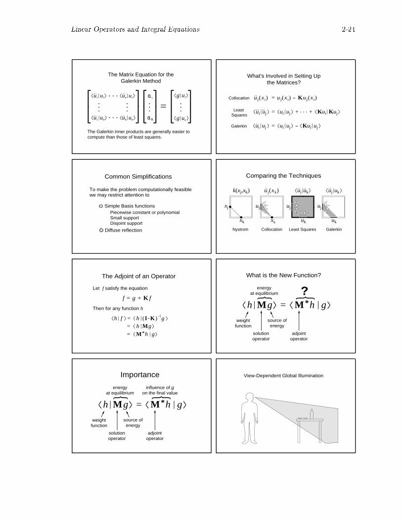
What's Involved in Setting Upthe Matrices?

Collocation

Galerkin

ui uj ui uj Kui Kuj+ . . . +=

ui uj ui uj Kui uj- =

u j(x i) u j(x i) - Ku j(x i)=

Least Squares

Common Simplifications

To make the problem computationally feasiblewe may restrict attention to

Simple Basis functionsPiecewise constant or polynomial

Diffuse reflection

Small supportDisjoint support

Comparing the Techniques

uj uk uj uku j(xk)k(xj,xk)

xj

xk

uj

xk uk uk

Nystrom Collocation Least Squares Galerkin

uj uj

The Adjoint of an Operator

h h (I -K ) -1g f

M*h g=

= h Mg=

Let f satisfy the equation

f = g + K f

Then for any function h

What is the New Function?

M*h g= h Mg

{ {

source ofenergy

weightfunction

solutionoperator

energyat equilibrium ?

adjointoperator

Importance

M*h g= h Mg

{ {

source ofenergy

weightfunction

solutionoperator

energyat equilibrium

influence of gon the final value

adjointoperator

View-Dependent Global Illumination


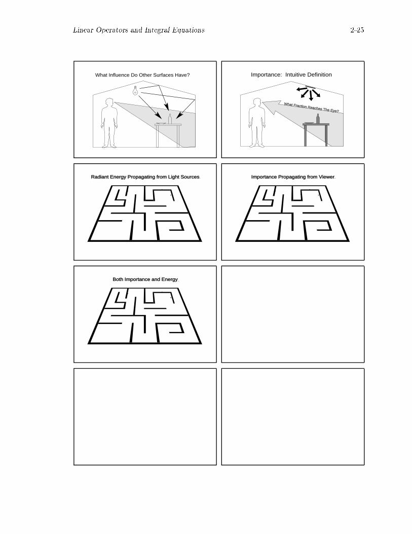
What Influence Do Other Surfaces Have?

What Fraction Reaches The Eye?

Importance: Intuitive Definition

Radiant Energy Propagating from Light Sources Importance Propagating from Viewer

Both Importance and Energy

linear operators and integral equations in global illumination

Documents