lecture notes on fourier integral operators: from … notes on fourier integral operators: from...

Lecture Notes onFourier Integral Operators:from local to global theory∗

Lorenzo ZanelliCentre de Mathematiques Laurent Schwartz

Ecole PolytechniqueRoute de Saclay 91120 Palaiseau

[email protected]

∗First and Preliminary Version!

“...The way out lay just in the possibility of attributing to the Hamilton principle,also, the operation of a wave mechanism on which the point-mechanical processes areessentially based, just as one had long become accustomed to doing in the case of phe-nomena relating to light and of the Fermat principle which governs them. Admittedly,the individual path of a mass point loses its proper physical significance and becomes asfictitious as the individual isolated ray of light. The essence of the theory, the minimumprinciple, however, remains not only intact, but reveals its true and simple meaningonly under the wave-like aspect, as already explained. Strictly speaking, the new theoryis in fact not new, it is a completely organic development, one might almost be temptedto say a more elaborate exposition, of the old theory.”

Erwin SchrodingerThe fundamental idea of wave mechanics

Nobel Lecture, December 12, 1933.

Contents

1 Introduction 4

2 Pseudodifferential Operators 52.1 Settings . . . . . . . . . . . . . . . . . . . . . . . . . . . . . . . . . . . 52.2 Quantization . . . . . . . . . . . . . . . . . . . . . . . . . . . . . . . . 6

3 Canonical transformations 73.1 Settings . . . . . . . . . . . . . . . . . . . . . . . . . . . . . . . . . . . 73.2 Generating functions . . . . . . . . . . . . . . . . . . . . . . . . . . . . 83.3 The graph of the Hamiltonian flow . . . . . . . . . . . . . . . . . . . . 11

4 Local theory of Fourier Integral Operators 154.1 Settings . . . . . . . . . . . . . . . . . . . . . . . . . . . . . . . . . . . 154.2 Properties . . . . . . . . . . . . . . . . . . . . . . . . . . . . . . . . . . 18

5 Global theory of Fourier Integral Operators 215.1 Preliminaries . . . . . . . . . . . . . . . . . . . . . . . . . . . . . . . . 215.2 Settings . . . . . . . . . . . . . . . . . . . . . . . . . . . . . . . . . . . 215.3 Characterization . . . . . . . . . . . . . . . . . . . . . . . . . . . . . . 23

6 Parametrices for the quantum evolution 246.1 Real and local phases . . . . . . . . . . . . . . . . . . . . . . . . . . . . 246.2 Complex and global phases . . . . . . . . . . . . . . . . . . . . . . . . . 256.3 Real and global phases . . . . . . . . . . . . . . . . . . . . . . . . . . . 27

L. Zanelli Introduction

1 Introduction

The aim of these Lecture Notes is to review the local and global theory of FourierIntegral Operators (FIO) as introduced by L. Hormander [16], [17] and subsequentlyimproved by J.J. Duistermaat [10] and F. Treves [29]. This is a wide and general theory,and thus we provide here only a short and comprehensive (but rigorous) description.From a general viewpoint, we can say that these operators naturally extend the setof Pseudodifferential Operators (PDO) and that this objective is realized by a linkwith the set of the canonical transformations and their graphs viewed as Lagrangiansubmanifolds of a symplectic manifold. In particular, the main idea is to require thatFIO are integral operators exhibiting Lagrangian distribution kernels.There exist meaningful applications of FIO in different frameworks, in particular to thestudy of hyperbolic type equations, and the related literature is quite large. In fact, asL. Hormander underlined in [17], the original local notion of FIO is due to P.D. Laxin the paper [20] where the objective was the study of the singularities of hyperbolicdifferential equations.In the last section of these Lecture Notes, we provide a resume the main results in thefirst papers as well as in the more recent ones involving the use of FIO to get local andglobal in time parametrices of the propagator of Schrodinger type equations.

Acknowledgements: I am very much grateful to S. Graffi, A. Parmeggiani, T. Paul for the

many useful discussions on semiclassical Analysis, and I am very much grateful to F. Cardin

for the many useful discussions on symplectic Geometry.

L. Zanelli Pseudodifferential Operators

2 Pseudodifferential Operators

In this section we provide the standard setting about the theory of PseudodifferentialOperators on Rn.

2.1 Settings

To begin, we recall the definition for the set of amplitudes functions.

Definition 2.1. Amplitudes Let m, ρ be real numbers with 0 ≤ ρ ≤ 1. We denote byΠmρ (R3n) the set of all a(x, y, ξ) ∈ C∞(R3n;C) such that for all multiorders α, β, γ and

some m′ satisfy

|∂αx∂βy ∂γξ a(x, y, ξ)| ≤ Cα,β,γ 〈z〉m−ρ |α+β+γ| 〈x− y〉m′+ρ |α+β+γ|,

where z := (x, y, ξ), 〈z〉 :=√

1 + |z|2 and Cα,β,γ > 0.

The set of Pseudodifferential Operators associated with the above amplitudes can beintroduced, as done by M.A. Shubin [32], in the following way

Definition 2.2. PDOLet a ∈ Πm

ρ (R3n;C), the associated PDO is defined as

A(u) := (2π)−n∫R2n

ei(x−y)·ξ a(x, y, ξ)u(y)dydξ, u ∈ S(Rn). (2.1)

It can be easily proved that the map A : S(Rn) −→ S(Rn), which is defined on theSchwartz space, is continuous by using an estimate of Ck-norms.

Looking at simbols a ∈ Πmρ (Rn

x ×Rnξ ;R) in the form a(x, ξ) :=

∑1≤j≤n

∑|α|≤m aα(x)ξαj

we localize a set of Differential Operators on Rn, since it holds A = a(x, ∂x).

About the L2(R2n)-boundedness for a class of PDO, we recall the well known Calderon-Vaillancourt Theorem (see for example [23]).

Theorem 2.3. Let a ∈ Πmρ (R3n) be such that ∂αz a ∈ L∞(R3n) for all α ∈ N. Then, the

operator A defined in (2.1) is continuous with respect to the topology induced by theL2(Rn)-norm and extends to a bounded operator on L2(Rn). Moreover,

‖A‖L2→L2 ≤ Cn∑|α|≤Mn

‖∂αz a‖∞ (2.2)

where Cn,Mn > 0 depend only on the dimension n.

L. Zanelli Pseudodifferential Operators

2.2 Quantization

In the framework of semiclassical Analysis (see for example A. Martinez [23]) we havethe following important notion

Definition 2.4. QuantizationLet 0 < ~ ≤ 1, 0 ≤ t ≤ 1. A family of quantizations of the classical observablesb ∈ Πm

ρ (R2n;R) reads as

Opt~(b)(u) := (2π~)−n∫R2n

ei~ (x−y)·ξ b((1− t)x+ ty, ξ)u(y)dydξ, u ∈ S(Rn).

The case t = 0 is the so-called “standard” (or left) quantization, the case t = 1/2 isknown as the “Weyl” quantization and usually reads OpW~ (b), whereas the case t = 1is the “right” quantization.

Remark 2.5. The Weyl quantization naturally arises in Quantum Mechanics thanks tothe link with the Heisemberg group (see for example G. Folland in [11]). Moreover, weremark that OpW~ (b) is particularly useful in semiclassical Analysis since it is simmetricwith respect to the L2(Rn) scalar product.

We now remind that the quantum evolution of an observable is closer and closer to itsclassical evolution as the Planck constant becomes negligible. This result is known inthe literature as the Egorov’s Theorem. In fact, it can be proved that the semiclassicalasymptotic expansion for the propagation of quantum observables OpW~ (b), for smoothHamiltonians growing at most quadratically at infinity, is uniformly dominated at anyorder by an exponential term whose argument is linear in time. In particular, it arisesnecessarily a time obstruction T (~) ' log (~−1) which is called the “Ehrenfest time”for the validity of this semiclassical approximation.To be more precise, let H ∈ C∞(R2n;R) be such that sup(x,ξ)∈Rn |∇2H(x, ξ)| < +∞,

and take the quantum propagator U~(t) := exp(−iOpW~ (H)t/~). Then, for t ∈ [0, TN(~))with TN(~) := −2 log (~)/(N − 1), we have the semiclassical asymptotics

U~(−t) OpW~ (b) U~(t) =N∑j=0

~jOpW~ (bj(t)) +RN(t) (2.3)

for suitable simbols bj(t) ∈ Πmρ (R2n;R) and

‖RN(t)‖L2→L2 ≤ CN (6n+1)N(−~ log (~))N . (2.4)

In particular, the lower order simbol reads b0(t, x, ξ) := b(φtH(x, ξ)), namely the classicalpropagation of the simbol b. Whereas the higher order terms bj(t, x, ξ) are determinedby the classical evolution but have a polynomial dependence on the derivatives of theflow φtH with respect to the variables (x, ξ) up to the order j − 1. About the precisesetting of bj we refer to D. Bambusi, S. Graffi and T. Paul [3].

L. Zanelli Canonical transformations and generating functions

3 Canonical transformations

3.1 Settings

Adopting standard notations, let M be a manifold and T ?M the corresponding cotan-gent bundle. We denote by ω = dp∧dx =

∑ni=1 dpi∧dxi the 2–form on T ?M that defines

its natural symplectic structure. As usual, a differomorphism C : T ?M −→ T ?M is acanonical transformation if the pull back of the symplectic form is preserved, namelythe condition C?ω = ω.We say that L ⊂ T ?M is a Lagrangian submanifold if

ω|L = 0, dim(L) = n =1

2dim(T ?M). (3.5)

A symplectic structure ω on T ?M × T ?M ∼= T ? (M ×M) is the twofold pull–back ofthe standard symplectic 2–form on T ?M defined as ω := pr?2ω − pr?1ω which in factequals ω = dp2 ∧ dx2 − dp1 ∧ dx1. Similarly, Λ ⊂ T ?M × T ?M is called Lagrangiansubmanifold of T ?M × T ?M if

ω|Λ = 0, dim(Λ) = 2n. (3.6)

A diffeomorphism C on T ∗Rn is canonical if and only if its graph

Λ = (y, ξ;x, p) ∈ T ∗M × T ∗M | (x, p) = C(y, ξ) (3.7)

is a Lagrangian submanifold with respect to the induced symplectic structure ω.We refer to an Hamiltonian as a C2-function H : T ?M −→ R. It can be esily provedthat the flow solving Hamilton’s equations on T ∗M

γ = J∇H(γ), γ(0) := γ0 ∈ T ?M,

is a one parameter group of canonical transformations

φtH : T ?M −→ T ?M, t ∈ R.

The global well defined character of the flow is guaranteed by the global uniformLipschitz behaviour of the Hamiltonian vector field XH := J∇H defined on T ?M . Inall the subsequent results involving Hamiltonian flows, if the particular form of H isnot specified, we will assume this general assumption.As we will see in the following sections, and in particualar in the last one, the localand global study of the time dependent family of Lagrangian submanifolds

Λt = (y, ξ;x, p) ∈ T ∗M × T ∗M | (x, p) = φtH(y, ξ) (3.8)

is very much important in classical mechanics and as a consequence in the semiclassicalanalysis of the related quantum flow.


3.2 Generating functions

We begin this subsection by recalling a well-known and important result of symplecticGeometry due to V.P. Maslov [25] and L. Hormander [16] which involves the localparametrization of arbitrary Lagrangian submanifolds.

Theorem 3.1. Local parametrization of Lagrangian submanifoldsLel M be a manifold and S ∈ C2(Mx × Rk

θ ;R). Let L ⊂ T ?M be the locus defined as

L := (x, p) ∈ T ?M | p = ∇xS(x, θ), 0 = ∇θS(x, θ) . (3.9)

Suppose that

rank(∇2xθS(x, θ) ∇2

θθS(x, θ))∣∣∣

L= max. (3.10)

Then, L is a Lagrangian submanifold of T ?M .Conversely, let L be a Lagrangian submanifold of T ?M and take

L → T ?M →M

λ 7→ j(λ) = (x, p) 7→ π(x, p) = x.

Then, for any z0 = (x0, p0) ∈ L there exists a local parametrization of type (3.9),namely

L ∩Br(z0) = (x, p) ∈ T ?M | p = ∇xS(x, θ), 0 = ∇θS(x, θ) .

where the dimension k fulfills

k ≥ dim(M)− rank[D(π j)(z0)].

Remark 3.2. We undeline that the Lagrangian submanifold L is the geometrical objectwhich is reasuming the local inverse functions of x 7→ ∇xS. In view of the aboveresult, we underline that the problem of the inversion of gradient maps is close tothe problem of inversion of the Legendre transformation. We can say that the abovefamily of functions S is a sort of weak analogue of the Hamiltonian function Legendrerelated to a Lagrangian function. In other words, the Lagrangian submanifold L can beinterpreted as a sort of multi-valued Legendre relation.

We introduce now the central objects of this section.

Definition 3.3. A generating function for a Lagrangian submanifold L ⊂ T ?Rn is aC1 function S : Rn × Rk −→ R such that

(i) L = (x, p) ∈ T ?Rn : p = ∇xS, 0 = ∇θS ,

(ii) rank(∇2xθS(x, θ) ∇2

θθS(x, θ))

= max.

The second condition is usually equivalently introduced by saying that zero (in Rk) isa regular value of the map (x, θ) 7−→ ∇θS(x, θ).


In a similar way, we have the following

Definition 3.4. A generating function for a Lagrangian submanifold Λ ⊂ T ?Rn×T ?Rn

is a C1 map S : Rn × Rn × Rk −→ R such that

(i) Λ = (x, p; y, ξ) ∈ T ?Rn × T ?Rn : p = ∇xS, ξ = −∇yS, 0 = ∇θS ,

(ii) zero (in Rk) is a regular value of the map (x, y, θ) 7−→ ∇θS(x, y, θ).

As we will see in the next section, the original setting of local FIO involves phase func-tions as generating functions which are positive-omogeneous with repect to θ of degreeone. On the other hand, a different class of generating functions naturally arises in sym-plectic geometry and as a consequence also in semiclassical Analysis (in particular, inthe Schrodinger framework). Indeed, we recall that J. C. Sikorav ([34]) introduced theimportant notion of generating function quadratic at infinity. In these Lecture Notes werefer to the similar setting used in the work of Theret [36], but involving not compactsetting.

Definition 3.5 (GFQI). A generating function S : Rn × Rk −→ R is called

weakly quadratic at infinity if there exists a C1-function Q : Rn × Rk −→ R inthe form Q(x, θ) := 〈Q(x)θ, θ〉, a C1 function 〈b(x), θ〉 and a C1-bounded c(x, θ)such that P (x, θ) := 〈Q(x)θ, θ〉+ 〈b(x), θ〉+ c(x, θ) such that

‖S(x, ·)− P (x, ·)‖C1(Rk) ≤ C, ∀x ∈ Rn. (3.11)

quadratic at infinity if (3.11) is fulfilled with Q(x) non degenerate.

exactly quadratic at infinity if S(x, θ) = 〈Q(x)θ, θ〉, with Q(x) non degenerateoutside of a compact set K ⊂ Rn. In particular, if Q(x) = Q, S is called special.

We remember that there exists three operations preserving generating functions:

Definition 3.6. Let S(x, θ) : Rn×Rk −→ R be a generating function for a Lagrangian

submanifold L. We say that S is obtained from S by

stabilization, if there exists a C1 non degenerate quadratic function 〈a(x)v, v〉,v ∈ Rh and S(x, θ, v) = S(x, θ) + 〈a(x)v, v〉.

fibered diffeomorphism, if there exists a regular θ : Rn × Rk −→ Rk such thatθ(x, ·) is a diffeomorphism and S(x, v) = S(x, θ(x, v)).

addition of constant, if S(x, θ) = S(x, θ) + C.

Remark 3.7. It is usual to consider the equivalence of two generating functions if theycan be made equal after a succession of these three operations. Moreover, the unique-ness of quadratic generating functions for a Lagrangian submanifold is often consideredwith respect to this notion of equivalence.


Now we recall the main results about existence and uniqueness of quadratic generatingfunctions of the graphs of Hamiltonian isotopies on the cotangent bundle of closedmanifolds M .

Theorem 3.8 (Sikorav [34]). Let L be a closed Lagrangian submanifold in T ?M whichadmits a generating function exactly quadratic at infinity, φtH : T ?M → T ?M anhamiltonian isotopy. Then φtHL also has a gfqi.

Theorem 3.9 (Viterbo [37]). Let us consider an hamiltonian isotopy φtH : T ?M →T ?M , and Lt = φtHOM . Assuming S1 and S2 are two generating functions exactlyquadratic at infinity for Lt, then they are equivalent.

Remark 3.10. We recall that Theret ([36]) proved, in the same setting of Thereom3.9, that any generating function quadratic at infinity is equivalent to a special one(see def. 3.5). This important fact implies that the previous two theorems still hold forgenerating functions quadratic at infinity.

Moreover, if we set a smooth H : T ?M → R, following Brunella [?] we underline thatwith an isometric embedding i : M → RN it can be defined a symplectic embeddingE : T ?M → T ?Rd such that there exists an extension of the Hamiltonian dynamics. Inwhat follows we state the precise result:

Theorem 3.11 (Brunella [4]). Let φtH : T ?M → T ?M be an hamiltonian isotopy, thenthere exists a symplectic embedding E : T ?M → T ?Rd and an Hamiltonian isotopyψtK : T ?Rd → T ?Rd, such that ∀t ∈ [0, T ]:

(i) E φtH = ψtK E

(ii) ψtK leaves invariant T ?Rd|i(B)

moreover, if V ⊂ Rd is a neighborhood of i(B), then we may choose every ψt withsupport contained in T ?RN |V .

In view of the above theorem, we underline the problem to determine smooth Hamilto-nians H : T ?Rn → R such that the graph of corresponding isotopies φtH : T ?Rn → T ?Rn

exhibit existence and uniqueness of generating functions quadratic at infinity. An an-swer to this problem is given in the paper [13], where it is enquired the constructionand equivalence of smooth global generating functions quadratic at infinity for theLagrangian graph

Λt = (y, ξ;x, p) ∈ T ∗Rn × T ∗Rn | (x, p) = φtH(y, ξ), (3.12)

namely S ∈ C1([0, T ]× R2n+k;R) such that

Λt = (x, p; y, ξ) ∈ T ?Rn × T ?Rn : p = ∇xS, ξ = −∇yS, 0 = ∇θS (3.13)

as in the setting of Definition 3.5.


3.3 The graph of the Hamiltonian flow

In this subsection we deal with the following class of Hamiltonian functions

Definition 3.12. H ∈ C∞(R2n;R) such that there exists an open set Ω ⊆ R2n whichis invariant under the Hamiltonian flow and such that for any α, β ∈ Zn+

sup|α|+|β|≥2

sup(x,p)∈Ω

|∂αx∂βpH(x, p)| < +∞.

For example, the class of confining mechanical Hamiltonian functions

H(x, p) :=1

2m|p|2 + V (x) (3.14)

where V ∈ C∞(Rn;R) is such that:

c1〈x〉d ≤ V (x) ≤ c2〈x〉d, 0 < c1 < c2, d ≥ 2, ∀ |x| ≥ R,

|∂αxV (x)| ≤ c〈x〉d−|α|, ∀ |α| ≥ 0.

We can also take the class of mechanical Hamiltonians with potentials V ∈ C∞(Rn;R)such that

supx∈Rn

|∇2V (x)| < +∞. (3.15)

We focus our attention on the graph of a Hamiltonian flow φtH : T ?Rn → T ?Rn

Λt :=

(y, η;x, p) ∈ T ?Rn × T ?Rn | (x, p) = φtH(y, η)

for H as in Definition 3.12 and time intervals [0, T ] arbitrary large. Our objective is todetermine a class of global generating functions for Λt, namely

Λt = (y, η;x, p) ∈ T ?Rn × T ?Rn | p = ∇xS, y = ∇ηS, 0 = ∇θS(t, x, η, θ)(3.16)

In order to do so, we follow a variational approach and in particular the so-calledAmann-Conley-Zhender reduction ([2], [9], [6], [38]).

First, we look at the boundary problem in the function space H1([0, T ];R2n) for theHamilton’s equation of motion:

γ(s) = J∇H(γ(s)); γx(t) = x, γp(0) = η. (3.17)

It can be easily seen that all the solutions of (3.17) belongs to the following set

Γ0(t, x, η) :=

(x−

∫ t

s

φx(τ) dτ ; η +

∫ s

0

φp(τ) dτ

) ∣∣∣ φ ∈ L2([0, T ];R2n)

(3.18)

Observe that the Hamilton-Helmholtz functional:

A[(γx, γp)] :=

∫ t

0

γp(s)γx(s)−H(γx(s), γp(s)) ds (3.19)


is well defined and continuous on the path space W 1,2([0, T ];R2n). Now define thefunction S : [0, T ]×R2n×L2 → R by the above functional evaluated on γ ∈ Γ0(t, x, η)

S(t, x, η, φ) := 〈γx(0), η〉+

∫ t

0


It has been proved in [6], [14] that

Λt =

(y, η;x, p) ∈ T ?Rn × T ?Rn | p = ∇xS, y = ∇ηS, 0 =

DSDφ

(t, x, η, φ)

where DS/Dφ stands for the Gateaux derivative. In view of this fact, we read theproblem (3.17) as a fixed point functional equation:

φ = G(t, x, η, φ) (3.21)

where G : [0, T ]× R2n × L2([0, T ];R2n)→ L2([0, T ];R2n) is given by

G(t, x, η, φx, φp) :=

(η

m+

1

m

∫ s

0

φp(τ) dτ,−∇V(x−

∫ t

s

φx(τ)dτ

))(3.22)

It can be easily seen that equation (3.21) is equivalent to the

0 =DSDφ

(t, x, η, φ)

Remark 3.13. This is an infinite dimensional setting, whereas we are looking forfinite dimensional generating functions of Λt. However, this gives the motivation andthe right variational approach that we are going to use in the subsequent part of thissection.

Before going further, we observe that for our class of Hamiltonians first of all we haveto localize the study of the Hamiltonian flow, the related graph and the above fixedpoint equation within the invariant set Ω:

Γ1(t, x, η) :=γ ∈ Γ0(t, x, η) | γ(s) ∈ Ω, ∀s ∈ [0, t]

(3.23)

and look at the equationφ = G(t, x, η;φ) (3.24)

selecting only the solutions of the problem (3.17) in the set Γ.Now, we set a finite dimensional ortogonal projector Pk : L2 → L2, define the dimensionK =: dim(PkL2) = 2n(2k + 1), indicate v ∈ PkL2 and θ ∈ RK the coordinates of v[θ]with respect a fixed ortonormal basis of PkL2. Define Qk := id − Pk and f ∈ QkL

2.Decompose equation (3.21) into the following

v = Pk G(t, x, η;φ) (3.25)

f = Qk G(t, x, η;φ) (3.26)

where v = Pkφ and f = Qkφ.We are now ready to recall the


Theorem 3.14. If the lower bound

k > C T 2 sup|α|+|β|≥2

sup(y,η)∈Ω

|∂αx∂βpH(y, η)|2 (3.27)

is satysfied, then there exists a unique smooth f = f(t, x, η, v)

f : [0, T ]× R2n × PkL2([0, T ];R2n)→ QkL2([0, T ];R2n)

solving the contraction equation on QkL2([0, T ];R2n):

f = Qk G(t, x, η; v + f)

Moreover, we have the L2-norm estimates

‖∂αx∂βη f(t, x, η, v)(·)‖L2 ≤ Cαβ(T )

for some Cαβ(T ) > 0 and v ∈ PkL2([0, T ];R2n).

The previous result allow to localize the finite space of curves

Definition 3.15. By the identification

φ(t, x, η, θ) := v[θ] + f(t, x, η, v[θ]) (3.28)

where θ ∈ RK are the coordinates of v ∈ PkL2([0, T ];R2n) with dimension

K = 2n · (2k + 1) (3.29)

we can reduce the space of curves (3.18) to the finite dimensional one

Γ2 :=

(x−

∫ t

s

φx(t, x, η, θ)(τ) dτ ; η +

∫ s

0

φp(t, x, η, θ)(τ) dτ

) ∣∣∣ θ ∈ RK

As a consequence, we realize the following inclusions:

Γ2(t, x, η) ⊂ Γ1(t, x, η) ⊂ Γ0(t, x, η) (3.30)

This fact allow a finite dimensional variational reduction of the Action functional:

Definition 3.16.

S(t, x, η, θ) := 〈γx(0), η〉+

∫ t

0


with γ = γ(t, x, η, θ) ∈ Γ(t, x, η).


Theorem 3.17. The function S as in (3.31) is a global generating function for

Λt :=

(y, η;x, p) ∈ Ω× Ω | (x, p) = φtH(y, η)

namely we have the parametrization:

Λt =

(y, η;x, p) ∈ Ω× Ω | p = ∇xS, y = ∇ηS, 0 = ∇θS(t, x, η, θ)

Moreover, it is fulfilled the rank condition:

rank(∇2xθS ∇2

ηθS ∇2θθS)∣∣∣

Λt

= max.

Remark 3.18. We remind that here we are dealing with phase functions obtained bya finite dimensional variational reduction of the Action functional. In this setting, weunderline that for mechanical Hamiltonians as in Definition 3.12, the transition betweenthe case of asymptotic quadratic potentials and the asymptotic polinomial potentials ofhigher order shows important features.

First, we observe that if d > 2 we can take the sublevel set

ΩE := (y, η) ∈ R2n | E0 < H(y, η) < E, E0 := inf(y,η)∈R2n

H(y, η).

Moreover, if E → +∞ then K(E) increases and the topology of the set ΓE in-volves the whole infinite dimensional space H1([0, T ];R2n).

Second, we observe that in the case d = 2 we can construction the phase functionnot depending on bounded energy sublevels. Indeed, recalling condition (3.27), inthis case the finite variational reduction (3.31) is globally well defined withoutrequiring the constraint of the curves into bounded ΩE.

Third, as in the case d = 2, the same holds true for smooth potentials onlysatisfying ‖∇2V ‖∞ < +∞, which is an assumption used in many papers involvingthe semiclassical analysis of Schrodinger type problems; for example this is thecase of smooth periodic potentials used for models in solid-state physics.

L. Zanelli Local theory of Fourier Integral Operators

4 Local theory of Fourier Integral Operators

Here we summarize the local theory of FIO, in particular we will refer to the booksof Hormander [16], [17], Duistermaat [10], Treves [29], where the reader can find theexhaustive exposure.

4.1 Settings

Let Ω ⊂ Rn be an open subset, it is customary to define E(Ω) := C∞(Ω) andD(Ω) := C∞0 (Ω) where C∞0 (Ω) :=

⋃K<<ΩDK and DK := u ∈ C∞(Ω) | supp u ∈ K

with K is a compact subset in the topology of Ω; it can be easily shown that they havethe structure of Frechet spaces. In this settings, E ′(Ω) and D′(Ω) are the sets of linearcontinuous functionals on these spaces.

Now we remember the definition of simbols space Smρ,δ (as originally introduced byHormander and also mainly used by Duistermaat). This is in fact a generalization ofthe simbols used in the standard theory of Pseudodifferential Operators.

Definition 4.1. SymbolsLet m, ρ, δ be real numbers with 0 ≤ ρ ≤ 1, 0 ≤ δ ≤ 1. Then we denote by Smρ,δ(Rn×RN)the set of all a ∈ C∞(Rn × RN) such that for every compact set K ⊂ X and allmultiorders α β the estimate

|DβxD

αθ a(x, θ)| ≤ Cα,β,K (1 + |θ|)m−ρ|α|+δ|β|, x ∈ K, θ ∈ RN ,

is valid for some constant Cα,β,K. The elements of Smρ,δ are called symbols of order mand type (ρ, δ). If ρ + δ = 1 we also use the notation Smρ , and when ρ = 1 and δ = 0we sometimes write only Sm and talk about symbols of order m. Finally we set

S∞ρ,δ := ∪m Smρ,δ, S−∞ρ,δ := ∩m Smρ,δ

We begin with the definition of Fourier Integrals, see [10], [16].

Definition 4.2. Fourier IntegralsLet Ω be open subset of Rn; the integral

Iϕ(au) =

∫Ω⊂Rn

∫RN

eiϕ(x,θ)a(x, θ)u(x) dx dθ, u ∈ C∞0

is absolutely convergent if ϕ is real, a ∈ Sµρ (Ω × RN) and µ + ρ < 0. In this caseu → Iϕ(au) is continuous on C0

0(Ω) and therefore define a distribution A on in Ω oforder 0.

We continue with the following two definitions, due to Hormander [16].


Definition 4.3. Phase functionsLet Ω be an open subet of Rn, N ∈ N; we define the class Φ of phase functions

φ : Ω× Ω× RN → R

such that:

(i) φ is real valued C∞ function in Ω× Ω× RN/0;

(ii) φ is positive-omogeneous with repect to θ of degree one.

Definition 4.4. Fourier Integral OperatorsLet consider a simbol a ∈ Smρ,δ, and a phase function φ ∈ Φ. Now we can define thecorresponding Fourier Integral Operator A on the functions u ∈ C∞0 (Ω):

Au(x) :=

∫Rn

∫RN

eiφ(x,y,θ)a(x, y, θ)dθ u(y)dy (4.32)

We say that A has oder m and type (ρ, δ).

Now we remember a result about linear operators and distribution theory that will beused in the next theorem.

Theorem 4.5. For every linear continuous operator A in the space S(Rn) there existsa family of tempered distributions A(x, ·) depending on the parameter x ∈ Rn such that

Av(x) = 〈A(x, y), v(y)〉 ∀x ∈ Rn, (4.33)

Moreover for every µ ∈ S ′(Rn), the map:

v 7−→ 〈µ,Av〉 = 〈µ(x), 〈A(x, y), v(y)〉〉 v ∈ S(Rn), (4.34)

is a tempered distribution.

Definition 4.6. The family of distributions A is said to be the Schwartz kernel of thelinear operator A.

We underline that Definition 4.4 is very much general, and for this reason it is usefulto add non-degenerate conditions on the class of phase functions Φ in order to provethe well defined setting of the FIO.Moreover we will see that many authors make different hypothesis on phase functionsin order to prove more properties about the related FIO.

With respect to this problem, we recall an Hormander’s result (see [16]).


Theorem 4.7. Existence and continuity

(i) If φ ∈ Φ has no critical points as function of (x, y, θ) with θ 6= 0 then the oscil-latory integral (4.32) exists in the sense of distributions. Moreover if

m+N < kρ, m+N < k(1− δ), (4.35)

then 〈Au, v〉 is a continuous bilinear form for the Ck0 topologies on u, v.

Moreover A is a continuous linear map from Ck0 (Ω) to D′k(Ω) wich has a distri-

bution kernel KA ∈ D′k(Ω× Ω) given by the oscillatory integral

KA(w) =

∫RN

eiφ(x,y,θ)a(y, θ)w(x, y)dxdydθ, (4.36)

(ii) If φ ∈ Φ has no critical points as function of (y, θ) with θ 6= 0, then the oscillatoryintegral (4.32) exists in the sense of distributions. When (4.35) is valid then A isa continuous linear map from Ck

0 (Ω) to C(Ω).If it is satisfied:

m+N + j < kρ, m+N + j < k(1− δ), (4.37)

then A is a continuous linear map from Ck0 (Ω) to Cj(Ω).

(iii) If φ ∈ Φ has no critical points as function of (x, θ) with θ 6= 0, then the adjoint ofA has the properties listed in (ii) so A is continuous map from E ′j(Ω) to D′k(Ω)when (4.37) is fulfilled. In particular A defines a continuous map from E ′(Ω) toD′(Ω)

(iv) Let Rφ be the set of all (x, y) ∈ Ω × Ω such that φ(x, y, θ) has no critical pointθ 6= 0 as a function of θ. Then

KA(x, y) =

∫RN

eiφ(x,y,θ)a(y, θ)dθ (4.38)

defines a function in C∞(Rφ) which is equal to the distribution (4.36) in Rφ. IfRφ = Ω × Ω, it follows that A is an integral operator with a C∞ kernel, so A isa continuous map of E ′(Ω) into C∞(Ω).

This theorem is still quite general and it turns out that it is useful to encrease thehypothesis made on the phase functions, in order to obtain more features, for examplecontinuity on C∞c (Ω) and moreover L2 local and global boundedness. With respect tothis aim we begin by reporting the following theorem due to Treves [29]:

Theorem 4.8. Consider the Fourier Integral Operator A as in definition (4.32) relatedto a simbol a ∈ Smρ,δ and a phase function φ ∈ Φ as in (4.3). We assume the non-degeneracy condition: dx,θφ and dy,θφ, the differentials of φ with respect to (x, θ) and(y, θ) respectively, do not vanish anywhere in Ω× Ω× RN/0.Then A is a continuous linear map from C∞c (Ω)→ C∞(Ω) which can be extended as acontinuous map E ′(Ω)→ D′(Ω).


Some recent papers of Ruzhansky and Sugimoto (see [26] and [27]) deal with L2-boundedness for FIO, within different hypothesis on phase functions and symbols.Here we provide a result on FIO directly generalizing a class of PDO.

Theorem 4.9. Let T be defined by

Tu(x) :=

∫Rn

∫Rn

ei(x·ξ+φ(y,ξ))a(x, y, ξ)u(y)dydξ (4.39)

Let φ ∈ C∞(R2n;R) be such that ∀|γ| ≥ 1∣∣∣det(∂x∂ξφ(x, ξ)

)∣∣∣ ≥ C > 0, (4.40)

|∂γξ φ(y, ξ)| ≤ Cγ〈y〉. (4.41)

Let a = a(x, y, ξ) ∈ C∞(Rn × Rn × Rn) be such that

|∂αx∂βy ∂γξ a(x, y, ξ)| ≤ Cαβγ〈x〉−α, (4.42)

for all α, β, γ. Then T is L2(Rn) - bounded.

4.2 Properties

Here we summarize some important features of FIO, in particular we report the equiv-alence of phase functions theorem, and another result with the proof that the compo-sition of two such operators is still of the same type. Moreover we will see how suitableequivalence classes of these operators are directly related to Lagrangian submanifolds,and it is exactly from this observation that arises the Global definition of Fourier Inte-gral Operators that will be drawed in the section.

For the following theorem and lemma I refer to Duistermaat [10].

Theorem 4.10. Equivalence of phase functionsSuppose ϕ(x, θ) and ϕ(x, θ) are nondegenerate phase functions at (x, θ0) ∈ Rn×RN\0and at (x, θ0) ∈ Rn × RN\0, with N and N suitable related. Let Γ and Γ be conic

neighborhoods of (x0, θ0) and (x0, θ0) such that Tϕ : Cϕ → Λϕ and Tϕ : Cϕ → Λϕ areinjective, respectively. If Λϕ = Λϕ then any Fourier Integral A, defined by the phasefunction ϕ and amplitude a ∈ Sµρ (Rn × RN), ρ > 1

2, with ess supp a contained in a

sufficently conic neighborhood of (x0, θ0) is equal to a Fourier Integral defined by the

phase function ϕ and an amplitude a ∈ Sµ+ 12

(N−N)ρ (Rn × RN)

The following lemma states exactly the suitable relation between N and N used in theprevious theorem.


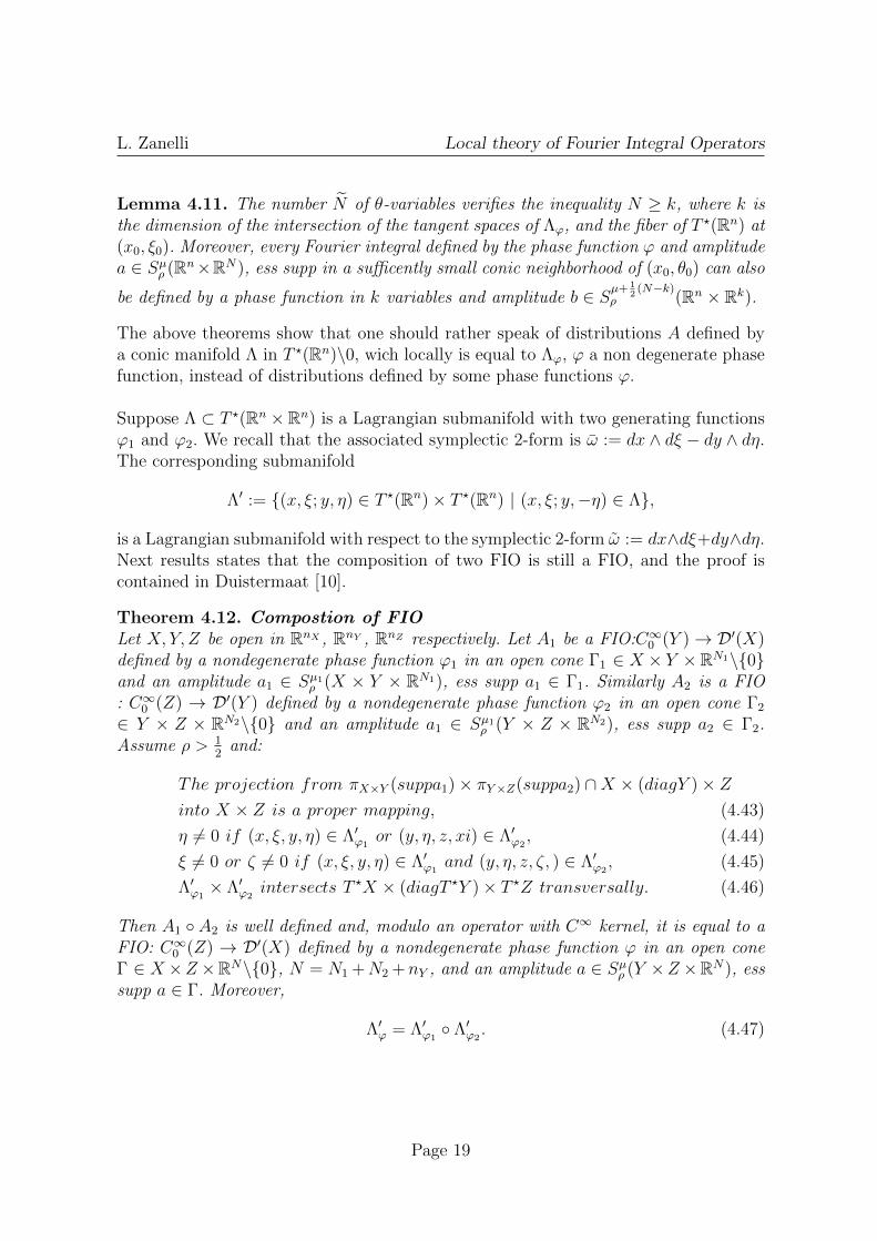
Lemma 4.11. The number N of θ-variables verifies the inequality N ≥ k, where k isthe dimension of the intersection of the tangent spaces of Λϕ, and the fiber of T ?(Rn) at(x0, ξ0). Moreover, every Fourier integral defined by the phase function ϕ and amplitudea ∈ Sµρ (Rn×RN), ess supp in a sufficently small conic neighborhood of (x0, θ0) can also

be defined by a phase function in k variables and amplitude b ∈ Sµ+ 12

(N−k)ρ (Rn × Rk).

The above theorems show that one should rather speak of distributions A defined bya conic manifold Λ in T ?(Rn)\0, wich locally is equal to Λϕ, ϕ a non degenerate phasefunction, instead of distributions defined by some phase functions ϕ.

Suppose Λ ⊂ T ?(Rn ×Rn) is a Lagrangian submanifold with two generating functionsϕ1 and ϕ2. We recall that the associated symplectic 2-form is ω := dx ∧ dξ − dy ∧ dη.The corresponding submanifold

Λ′ := (x, ξ; y, η) ∈ T ?(Rn)× T ?(Rn) | (x, ξ; y,−η) ∈ Λ,

is a Lagrangian submanifold with respect to the symplectic 2-form ω := dx∧dξ+dy∧dη.Next results states that the composition of two FIO is still a FIO, and the proof iscontained in Duistermaat [10].

Theorem 4.12. Compostion of FIOLet X, Y, Z be open in RnX , RnY , RnZ respectively. Let A1 be a FIO:C∞0 (Y )→ D′(X)defined by a nondegenerate phase function ϕ1 in an open cone Γ1 ∈ X × Y ×RN1\0and an amplitude a1 ∈ Sµ1ρ (X × Y × RN1), ess supp a1 ∈ Γ1. Similarly A2 is a FIO: C∞0 (Z) → D′(Y ) defined by a nondegenerate phase function ϕ2 in an open cone Γ2

∈ Y × Z × RN2\0 and an amplitude a1 ∈ Sµ1ρ (Y × Z × RN2), ess supp a2 ∈ Γ2.Assume ρ > 1

2and:

The projection from πX×Y (suppa1)× πY×Z(suppa2) ∩X × (diagY )× Zinto X × Z is a proper mapping, (4.43)

η 6= 0 if (x, ξ, y, η) ∈ Λ′ϕ1or (y, η, z, xi) ∈ Λ′ϕ2

, (4.44)

ξ 6= 0 or ζ 6= 0 if (x, ξ, y, η) ∈ Λ′ϕ1and (y, η, z, ζ, ) ∈ Λ′ϕ2

, (4.45)

Λ′ϕ1× Λ′ϕ2

intersects T ?X × (diagT ?Y )× T ?Z transversally. (4.46)

Then A1 A2 is well defined and, modulo an operator with C∞ kernel, it is equal to aFIO: C∞0 (Z) → D′(X) defined by a nondegenerate phase function ϕ in an open coneΓ ∈ X ×Z ×RN\0, N = N1 +N2 +nY , and an amplitude a ∈ Sµρ (Y ×Z ×RN), esssupp a ∈ Γ. Moreover,

Λ′ϕ = Λ′ϕ1 Λ′ϕ2

. (4.47)


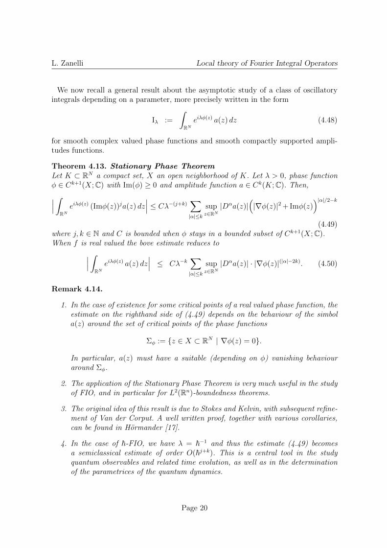
We now recall a general result about the asymptotic study of a class of oscillatoryintegrals depending on a parameter, more precisely written in the form

Iλ :=

∫RN

eiλφ(z) a(z) dz (4.48)

for smooth complex valued phase functions and smooth compactly supported ampli-tudes functions.

Theorem 4.13. Stationary Phase TheoremLet K ⊂ RN a compact set, X an open neighborhood of K. Let λ > 0, phase functionφ ∈ Ck+1(X;C) with Im(φ) ≥ 0 and amplitude function a ∈ Ck(K;C). Then,∣∣∣ ∫

RN

eiλφ(z) (Imφ(z))ja(z) dz∣∣∣ ≤ Cλ−(j+k)

∑|α|≤k

supz∈RN

|Dαa(z)|(|∇φ(z)|2 + Imφ(z)

)|α|/2−k(4.49)

where j, k ∈ N and C is bounded when φ stays in a bounded subset of Ck+1(X;C).When f is real valued the bove estimate reduces to∣∣∣ ∫

RN

eiλφ(z) a(z) dz∣∣∣ ≤ Cλ−k

∑|α|≤k

supz∈RN

|Dαa(z)| · |∇φ(z)|(|α|−2k). (4.50)

Remark 4.14.

1. In the case of existence for some critical points of a real valued phase function, theestimate on the righthand side of (4.49) depends on the behaviour of the simbola(z) around the set of critical points of the phase functions

Σφ := z ∈ X ⊂ RN | ∇φ(z) = 0.

In particular, a(z) must have a suitable (depending on φ) vanishing behaviouraround Σφ.

2. The application of the Stationary Phase Theorem is very much useful in the studyof FIO, and in particular for L2(Rn)-boundedness theorems.

3. The original idea of this result is due to Stokes and Kelvin, with subsequent refine-ment of Van der Corput. A well written proof, together with various corollaries,can be found in Hormander [17].

4. In the case of ~-FIO, we have λ = ~−1 and thus the estimate (4.49) becomesa semiclassical estimate of order O(~j+k). This is a central tool in the studyquantum observables and related time evolution, as well as in the determinationof the parametrices of the quantum dynamics.

L. Zanelli Global theory of Fourier Integral Operators

5 Global theory of Fourier Integral Operators

In this section we report two global, namely intrinsic, definitions of FIO, due toHormander [16] and Duistermaat [10].Duistermaat provide a direct generalization of local definition, moreover he establish acaracterization of the set of FIO associated to a Lagrangian submanifold.Hormander provides a very general formulation for a Fourier Integral Operator that,on the other hand, it is not so easy to connect with local definition.

5.1 Preliminaries

Let V be an n-dimensional vector space over R, ΛnV the space of the n-vectors in V ,defined as the dual of the vector space of the n-linear alternanting forms: V n → R.ΛnV is one dimensional over R. For any α ∈ R we call a complex valued density of orderα each mapping ρ : ΛnV \0 → C such that ρ(λw) = |λ|αρ(w) for each w ∈ ΛnV \0,λ ∈ R\0. The space of all densities of order α is 1-dimensional over C and will bedenoted by Ωα(V ).Now let X a n-dimensional C∞ manifold. The Ωx(T

?xX), x ∈ X, are the fibers of a C∞

complex line bundle Ωα(X) over X in a natural way. A C∞ density on X of order α isnow defined as a C∞ section ρ : X → Ωα(X). The space of C∞ densities on X of orderα will be denoted by C∞(X,Ωα). Note that after the choice of of a nowhere vanishingstandard density of order α, the space C∞(X,Ωα) can be identified with C∞(X). Usinga partition of unity it is always contruct a strictly positive C∞ density of order α onX if X is paracompact.If ρ ∈ C∞(X,Ωα), σ ∈ C∞(X,Ωβ) then pointwise multiplication leads to a productρ · σ ∈ C∞(X,Ωα+β). In particular

(ρ, σ)→∫

ρ · σ dx

defines a continuous bilinear form on C∞(X,Ωα)×C∞0 (X,Ω1−α) so σ →∫ρ·σ dx is an

element of (C∞0 (X,Ω1−α))′ that will be also denoted by ρ. It follows that we have a con-tinuous embedding: C∞(X,Ωα)→ (C∞0 (X,Ω1−α))′, and for this reason (C∞0 (X,Ω1−α))′

is called the space D′(X,Ωα) of distribution densities of order α.

5.2 Settings

By following Duistermaat [10], and Hormander [16], here we report the Global definitionof Fourier Integrals and Fourier Integral Operators.To begin we remember that, in the local definition, a Fourier Integral is an integralthat assume the form:

Iϕ(au) =

∫Ω⊂Rn

∫RN

eiϕ(x,θ)a(x, θ)u(x) dx dθ, u ∈ C∞0


where Ω is an open subset of Rn. It is absolutely convergent if ϕ is real, a ∈ Sµρ (Ω×RN)and µ + ρ < 0. In this case u→ Iϕ(au) is continuous on C0

0(Ω) and therefore define adistribution A on in Ω of order 0.

While in the global setting we have the following (see [10]):

Definition 5.1. Global Fourier IntegralsLet X be an n-dimensional smooth manifold, Λ an immersed conic Lagrangian subman-ifold in T ?(X)\0. A Global Fourier Integral of order m and type ρ by Λ is a distribution

A ∈ D′(X,Ω 12 ) such that

A =∑j∈J

Aj, (5.51)

where Aj ∈ D′(X,Ω12 ) with locally finite supp Aj, and Aj is a FIO defined by a

nondegenerate phase function ϕj on a open cone Γj in X × RNj such that (x, θ) 7→(x, dxϕj(x, θ)) is a diffeomorphims from Cφj = (x, θ) ∈ Γj | dθϕj(x, θ) = 0 onto an

open cone in Λ. For the amplitude aj it is required that aj ∈ Sm−Nj/2+n/4(X × RNj),cone supp aj ⊂ Γj.The space of all such Fourier integrals will be denoted by Imρ (X,Λ).

Now we refer to Hormander [17], and I remember the following definition:

Definition 5.2. Let X be a C∞ manifold with dimX = n, and Y a submanifold ofX. The space Im(X, Y ;E) of conormal distribution sections of vector bundle E is thelargest subspace of ∞H loc

−m−n/4(X,E), which is left invarant by all first order differentialoperators tangent to the submanifold Y .

It has proved (see [16], Th. 18.2.12) that it is even invariant under first order Pseu-dodifferential operators from E to E with principal symbol vanishing on the conormalbundle of Y . The definition is therefore applicable with no change to any Lagrangianmanifold:

Definition 5.3. Lagrangian DistributionsLet X be a C∞ manifold with dimX = n, and Λ ⊂ T ?X/0 a C∞ closed conic La-grangian submanifold, E a C∞ vector bundle over X. Then the space Im(X,Λ;E) ofLagrangian distributions of E, of order m, is defined as the set of all u ∈ D′(X,E)such that:

L1...LNu ∈ ∞H loc−m−n/4(X,E) (5.52)

for all N and all properly supported Lj ∈ Ψ1(X;E,E) with principal symbols L0j van-

ishing on Λ.

Definition 5.4. Let X, Y be two C∞ manifolds and E,F two complex vector bundleson X, Y . Then every D′(X × Y,C ′; ΩX×Y ⊗Hom(F,E)) defines a continuous map

A : C∞0 (Y,Ω12Y ⊗ F )→ D′(X,Ω

12Y ⊗ E) (5.53)

and conversely.


Here the fiber of the vector bundle Hom(F,E) at (x, y) consists of the linear maps Fyto Ex. In particular if Λ is a conic Lagrangian submanifold of T ?(X × Y )\0 we canidentify Im(X × Y,Λ; ΩX×Y ⊗Hom(F,E)) with a space of such maps.If we have Λ ⊂ T ?(X)\0×T ?(Y )\0 then it follows (see [16], Th. 25.1.2) that A is evencontinuous map from C∞0 (Y ) to C∞(X) which can be extended to a continuous mapfrom E ′ to D′ with

WF (Au) = C(WF (u)) u ∈ E ′(Y,Ω12Y ⊗ F ), (5.54)

whereC = Λ′ = (x, ξ, y, η) ∈ T ?(X)\0× T ?(Y )\0 ; (x, ξ, y, η) ∈ Λ (5.55)

is a canonical relation from T ?(X)\0 to T ?(X)\0. We call Λ = C ′ the twisted canonicalrelation.

Definition 5.5. Global Fourier Integral OperatorsLet C be a homogeneous canonical relation from T ?(Y )\0 to T ?(Y )\0 wich is closed inT ?(X × Y )\0 and let E,F be vectors bundles on X, Y . Then the operators with kernelbelonging to Im(X × Y,C ′; ΩX×Y ⊗Hom(F,E)) are called Fourier Integral Operatorsof order m from sections of F to sections of E, associated with the canonical relationC.

5.3 Characterization

Here I report a characterization, due to Duistermaat [10], about the set of FuorierIntegrals associated to a fixed Lagrangian submanifold of T ?(Rn).

Definition 5.6. Principal symbolFor a FIO A of order a defined by nondegenerate phase function ϕ and amplitude

a ∈ Sm−Nj/2+n/4ρ (X × RN), the principal symbol of order m is the element in

Sm+n/4ρ (Λ,Ω

12 ⊗ L)/Sm+n/4+1−2ρ

ρ (Λ,Ω12 ⊗ L), (5.56)

given byΛ 3 α 7→ eiψ(π(α),α)〈ue−iψ(x,α), A〉. (5.57)

Here L is the complex Keller Maslov line bundle of Λ (see Keller...). While Λ = Λϕ

is the conic Lagrangian manifold in T ?(X)\0 defined by ϕ. Sµρ (Λ,Ω12 ⊗ L) denotes the

symbol space of sections of the complex line bundle Ω12 ⊗ L over Λ, of growh order µ.

Moreover, u ∈ C∞0 (X × Λ) and ψ ∈ C∞(X × Λ), ψ(x, α) is homogeneous of degree 1in α and the graph x 7→ dxψ(x, α) intersects Λ transversally at α. Regarding (5.56) asa function of u and ψ, it becomes an element of (5.56).

With respect to these definitions we have the following results:

Theorem 5.7. If the immersion Λ 7→ T ?(X)\0 is proper and injective (that is anembedding), then the mapping A 7→ principal symbol of A, is an isomorphism:

Imρ (X,Λ)/Imρ (X,Λ)→ Sm+n/4ρ (Λ,Ω

12 ⊗ L)/Sm+n/4+1−2ρ

ρ (Λ,Ω12 ⊗ L) (5.58)

L. Zanelli Parametrices for the quantum evolution

6 Parametrices for the quantum evolution

Here we summurize some recents papers, about the use of global FIO with non omo-geneous phase functions to represent solutions of Schrodinger equations.From a general viewpoint, we can mainly divide the large related literature into threeparts. More precisely, the papers involving the use of oscillatory integrals with local intime and real phases, with the global in time and complex phases and finally with theglobal in time and real phases.In particular, about the first approach we refer to the papers of J. Chazarain [8], D.Fujiwara [12], Kitada and Hitoshi Kumano-go [18]. About the second appoach we referto A. Hassel and J. Wunsch [15], A. Laptev and I.M. Sigal [21], L. Kapitansky and Y.Safarov [19], T. Swart and V. Rousse [33], D. Robert [30]. About the last approach werefer to S. Graffi and L. Z. [14], L. Z. [40].

6.1 Real and local phases

In the local in time approach to the study of the Schrodinger equation (see for exampleJ. Chazarain [8], D. Fujiwara [12], Kitada and Hitoshi Kumano-go [18]), the objectiveis the study of the problem

i~∂tψ(t, x) = − ~2

2m∆xψ(t, x) + V (x)ψ(t, x) (6.59)

ψ(0, x) = ϕ(x) ∈ S(Rn),

with |∂αxV (x)| ≤ C, |α| = 2, for the time interval t ∈ [0, T0) where T0 is the first timeof appearence of the caustics phenomena in the phase space (see for example [1], [39]).Roughly speaking, the graph of the Hamiltonian flow can be globally parametrized witha generating function without θ-auxiliary parameters. Within this local in time setting,it can be constructed approximated parametrices for the Schrodinger propagator in theso-called WKB semiclassical asymptotics,

ψ(t, x) = (U~(t)ϕ)(x) =

∫Rn

U~(t, x, η)ϕ~(η)dη

where ϕ~(η) is the ~-Fourier transform of the initial datum. Obviously, it can be equiv-alently studied the fundamental solution of the above problem, namely U~(t, x, y). Thefirst equation naturally arising is the evolutive Hamilton-Jacobi equation

|∇xS|2

2m(t, x, η) + V (x) + ∂tS(t, x, η) = 0 (6.60)

with the initial condition S(0, x, η) := x · η.The second equation is the coupled transport equation,

∂tρ0 +1

m∇xS ∇xρ0 +

1

2m∆xS ρ0 = 0, (6.61)


with the initial condition ρ0(0, x, η) := 1.The third equation is a recoursive transport type equation

∂tρj +1

m∇xS ∇xρj +

1

2m∆xS ρj =

i

2m∆xρj−1, (6.62)

with initial condition ρj(0, x, η) := 0, j ∈ N, j ≥ 1.We are now ready to provide the family of operators

UN,~(t)ϕ := (2π~)−nN∑j=0

~j∫Rn

ei~S(t,x,η) ρj(t, y, η)ϕ~(η) dη (6.63)

which satisfies, for t ∈ [0, T0), the estimate

‖U~(t)− UN,~(t)‖L2→L2 ≤ RN(T0)~N+1.

In order to construct a parametrices for U~(t) with t ∈ [0, T ] for T ≥ T0, we recall thesemigroup property,

U~(t) = U~

(t

M

)M, M := [T/T0].

Hence, for t ∈ [0, T ] it holds∥∥∥U~(t)− UN,~(t

M

)M ∥∥∥L2→L2

≤ RN(T ) ~N+1.

6.2 Complex and global phases

In the work of Laptev and Sigal it is considered an Hamiltonian function H(t, x, ξ) realand smooth on R× T ?Rn, it is assumed that there are m > 0 and Cµν > 0 such that:for every (t, x) ∈ R× Rn

|∂µx∂νξH(t, x, ξ)| < Cµν(1 + |ξ|)m.

Let H~(t) be the ~-PDO with symbol H, i.e.

H~(t)f = (2π~)−n∫R2n

H(t, x, ξ)ei~ (x−y)·ξf(y)dydξ,

defined on the functions f ∈ C∞0 (Rn). Let Ω ⊆ R2n be an open bounded set and XΩ

the characteristic function; the associated PDO reads

XΩf = (2π~)−n∫R2n

XΩ(y, η)ei~ (x−y)·ηf(y)dydη,

Within this settings, it is considered the family of operators U~(t) solving the Scrodingerequation in the functional form:

i~∂tU~(t) = H~(t) U~(t), (6.64)

U~(0) = I. (6.65)


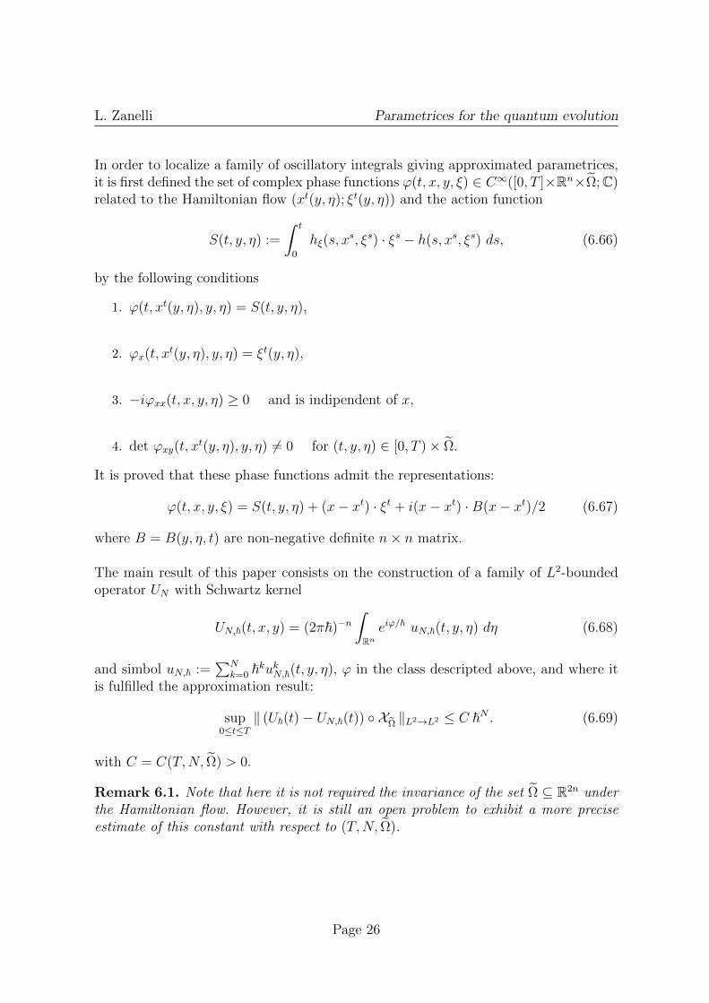
In order to localize a family of oscillatory integrals giving approximated parametrices,it is first defined the set of complex phase functions ϕ(t, x, y, ξ) ∈ C∞([0, T ]×Rn×Ω;C)related to the Hamiltonian flow (xt(y, η); ξt(y, η)) and the action function

S(t, y, η) :=

∫ t

0

hξ(s, xs, ξs) · ξs − h(s, xs, ξs) ds, (6.66)

by the following conditions

1. ϕ(t, xt(y, η), y, η) = S(t, y, η),

2. ϕx(t, xt(y, η), y, η) = ξt(y, η),

3. −iϕxx(t, x, y, η) ≥ 0 and is indipendent of x,

4. det ϕxy(t, xt(y, η), y, η) 6= 0 for (t, y, η) ∈ [0, T )× Ω.

It is proved that these phase functions admit the representations:

ϕ(t, x, y, ξ) = S(t, y, η) + (x− xt) · ξt + i(x− xt) ·B(x− xt)/2 (6.67)

where B = B(y, η, t) are non-negative definite n× n matrix.

The main result of this paper consists on the construction of a family of L2-boundedoperator UN with Schwartz kernel

UN,~(t, x, y) = (2π~)−n∫Rn

eiϕ/~ uN,~(t, y, η) dη (6.68)

and simbol uN,~ :=∑N

k=0 ~kukN,~(t, y, η), ϕ in the class descripted above, and where itis fulfilled the approximation result:

sup0≤t≤T

‖ (U~(t)− UN,~(t)) XΩ ‖L2→L2 ≤ C ~N . (6.69)

with C = C(T,N, Ω) > 0.

Remark 6.1. Note that here it is not required the invariance of the set Ω ⊆ R2n underthe Hamiltonian flow. However, it is still an open problem to exhibit a more preciseestimate of this constant with respect to (T,N, Ω).


6.3 Real and global phases

Let us consider the Schrodinger equation:

i~∂tψ(t, x) = − ~2

2m∆ψ(t, x) + V (x)ψ(t, x), (6.70)

ψ(0, x) = ϕ(x),

where ϕ ∈ S(Rn) and the confining potential V ∈ C∞(Rn;R) is such that:

c1〈x〉d ≤ V (x) ≤ c2〈x〉d, 0 < c1 < c2, d ≥ 2, ∀ |x| ≥ R,

|∂αxV (x)| ≤ c〈x〉d−|α|, ∀ |α| ≥ 0.

Our objective is to determine, for arbitrary large time intervals t ∈ [0, T ], a family ofsemiclassical series of global Fourier Integral Operators for the one parameter unitarytransformations U(t) := e−iHt/~ where H = − ~2

2m∆ + V (x). More precisely, in this

general setting we make a phase-space localization of the propagator within sublevelsof the energy function H(x, p) := 1

2m|p|2 + V (x). In fact, we follow a similar approach

with respect to the paper of Laptev and Sigal in [21], by looking at bounded sets whichare invariant under the Hamiltonian flow,

ΩE := (y, η) ∈ R2n | E0 < H(y, η) < E, E0 := inf(y,η)∈R2n

H(y, η) < E,

and defining the related Pseudodifferential operators:

XEϕ := (2π~)−n∫R2n

ei~ 〈x−y,η〉χΩE

(y, η)ϕ(y)dydη.

The aim is to exhibit semiclassical approximations for U(t) XE through a family ofglobal Fourier Integral Operators.We are now ready to state the main result of the paper

Theorem 6.2. For all E > E0, N ≥ 0 and t ∈ [0, T ] there exists a series of L2-boundedglobal Fourier Integral Operators

Uj,E(t)ϕ(x) := (2π~)−n+j

∫R2n

∫Rk

ei~SE(t,x,η,θ)−〈y,η〉ρj,E(t, x, y, η, θ)dθϕ(y)dydη, (6.71)

such that the following remainder estimate fulfills∥∥∥U(t) XE −N∑j=0

Uj,E(t)∥∥∥L2→L2

≤ CN(T )~N+1. (6.72)

with CN(T ) not depending on the energy value. The phase SE belongs to a class of globalgenerating functions for the graph of the Hamiltonian flow φtH : R2n → R2n within the

bounded energy set ΩE, namely:

ΛEt :=

(y, η;x, p) ∈ ΩE × ΩE | (x, p) = φtH(y, η)

=

(y, η;x, p) ∈ ΩE × ΩE | p = ∇xSE, y = ∇ηSE, 0 = ∇θSE

(6.73)


where θ ∈ Rk and the dimension must fulfill the lower bound:

k > 2n+Kd,E,N T 4 (6.74)

where KE,N,d is shown in Section 3.3. The zero order simbol ρ0 ∈ C∞([0, T ] × R3n ×Rk;R) belongs to a class of solutions of the transport equation written in the followinggeometrical setting:

∂tρ0,E +1

m∇xSE ∇xρ0,E +

1

2m∆xSE ρ0,E = 0, ∇θSE = 0, (6.75)

where the initial condition ρ0,E(0, x, y, η, θ) := σ(θ)χΩE(y, η) is arbitrary fixed with a

probability measure:

σ ∈ S(Rk;R+),

∫Rk

σ(θ)dθ = 1, σ(θ) ≤ cd e−|θ|d . (6.76)

The higher order simbols ρj,E ∈ C∞([0, T ]×R3n×Rk;R) belongs to a class of solutionsof the following recoursive transport equations:

∂tρj,E +1

m∇xSE ∇xρj,E +

1

2m∆xSE ρj,E =

i

2m∆xρj−1,E, ∇θSE = 0, (6.77)

with initial condition ρj,E(0, x, y, η, θ) = 0, ∀j ≥ 1.

In the asymptotic quadratic case d = 2, we can deal with a global FIO framework notdepending on the energy. Indeed, in this case there exists a global generating functionS not depending on the energy E and with finite auxiliary variables θ ∈ Rk with globallower bound

k > 2n+ KNT4. (6.78)

This fact allow a construction as in the previous theorem, but now without the Pseu-dodifferential operator XE and with simbols not depending on y-variables. We candetermine semiclassical series of global FIO directly representing the ~-Fourier trans-form F~ of the foundamental solution of the propagator.

Theorem 6.3. In the case d = 2, for all N ≥ 0 and t ∈ [0, T ] we have a series ofL2-bounded global Fourier Integral Operators:

Uj(t)ϕ(x) = (2π~)−n+j

∫Rn

∫Rk

ei~S(t,x,η,θ)ρj(t, x, η, θ)dθϕ~(η)dη, (6.79)

where ϕ~ := F~ϕ, and the remainder fulfills

∥∥∥U(t)−N∑j=0

Uj(t)∥∥∥L2→L2

≤ CN(T )~N+1. (6.80)


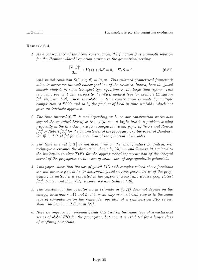
Remark 6.4.

1. As a consequence of the above construction, the function S is a smooth solutionfor the Hamilton-Jacobi equation written in the geometrical setting:

|∇xS|2

2m+ V (x) + ∂tS = 0, ∇θS = 0, (6.81)

with initial condition S(0, x, η, θ) = 〈x, η〉. This enlarged geometrical frameworkallow to overcome the well known problem of the caustics. Indeed, here the globalsimbols simbols ρj solve transport type equations in the large time regime. Thisis an improvement with respect to the WKB method (see for example Chazarain[8], Fujiwara [12]) where the global in time construction is made by multiplecomposition of FIO’s and so by the product of local in time simbolds, which notgives an intrinsic approach.

2. The time interval [0, T ] is not depending on ~, so our construction works alsobeyond the so called Ehrenfest time T (~) ' −c log ~; this is a problem arisingfrequently in the literature, see for example the recent paper of Swart and Rousse[33] or Robert [30] for the parametrices of the propagator, or the paper of Bambusi,Graffi and Paul [3] for the evolution of the quantum observables.

3. The time interval [0, T ] is not depending on the energy values E. Indeed, ourtechnique overcomes the obstruction shown by Yajima and Zang in [31] related tothe limitation in time T (E) for the approximated representation of the integralkernel of the propagator in the case of same class of superquadratic potentials.

4. This paper shows that the use of global FIO with complex valued phase functionsare not necessary in order to determine global in time parametrices of the prop-agator, as instead it is suggested in the papers of Swart and Rousse [33], Robert[30], Laptev and Sigal [21], Kapitansky and Safarov [19].

5. The constant for the operator norm estimate in (6.72) does not depend on the

energy, invariant set Ω and ~; this is an improvement with respect to the sametype of computation on the remainder operator of a semiclassical FIO series,shown by Laptev and Sigal in [21].

6. Here we improve our previous result [14] bsed on the same type of semiclassicalseries of global FIO for the propagator, but now it is exhibited for a larger classof confining potentials.

L. Zanelli References

References

[1] B. Aebischer. M. Borer, M. Kalin, Ch. Leuenberger, H. M. Reimann, Symplec-tic geometry. An introduction based on the seminar in Bern, 1992. Progress inMathematics, 124. Birkhauser Verlag, Basel, 1994.

[2] H. Amann, E. Zehnder, Periodic solutions of asymptotically linear hamiltoniansystems, Manuscr. Math. (1980), 32, 149–189.

[3] D. Bambusi, S. Graffi, T. Paul: Long time semiclassical approximation of quantumflows: a proof of the Ehrenfest time. Asymptotic analysis, 2 (1999), pp 149-160.

[4] M. Brunella, On a theorem of Sikorav. Enseign. Math. (2) 37 (1991), no. 1-2,83–87.

[5] J. Butler, Global h Fourier Integral Operators with complex-valued phase func-tions, Bull. Lond. Math. Soc. 34 (2002) 479-489.

[6] F. Cardin, The global finite structure of generic envelope loci for HamiltonJacobiequations, J. Math. Phys. 43(1) (2002) 417430.

[7] M. Chaperon, On generating families. The Floer memorial volume, 283–296, Progr.Math., 133, Birkhuser, Basel, 1995.

[8] J.Chazarain, Spectre d’un hamiltonien quantique et mecanique classique. Comm.Partial Differential Equations 5, no. 6, 595–644, 1980.

[9] C.Conley, E.Zehnder, A global fixed point theorem for symplectic maps and subhar-monic solutions of Hamiltonian equations on tori. In Nonlinear functional analysisand its applications, Part 1 (Berkeley, Calif., 1983), volume 45 of Proc. Sympos.Pure Math., pages 283 - 299. Amer. Math. Soc., Providence, RI, 1986.

[10] J.J. Duistermaat, Fourier integral operators, Birkhauser, 1996.

[11] G. Folland: Harmonic Analysis in Phase Space, Annals of Mathematics Studies122, Princeton University Press 1989

[12] D. Fujiwara, A construction of the fundamental solution for the Schrodinger equa-tion. J. Analyse Math. 35 (1979), 4196.

[13] P. Guiotto, L. Zanelli: The Geometry of Generating Functions for a class of Hamil-tonian flows in the non compact case, Journal of Geometry and Physics, vol. 60,1381-1401, 2010.

[14] S. Graffi, L. Zanelli, The geometric approach to the Hamilton-Jacobi equationand global parametrices for the Schrodinger propagator. Reviews in Mathemati-cal Physics, vol. 23, issue 9, 969-1008, 2011.


[15] A. Hassel, J. Wunsch, The Schrodinger propagator for scattering metrics, Annalsof Mathematics, 162 (2005), 487-523.

[16] L. Hormander, Fourier integral operators. I. Acta Math. 127 (1971), No. 1-2,79–183.

[17] L. Hormander, The Analysis of Linear Partial Differential Operators IV, SpringerVerlag, New York 1984.

[18] Kitada, Hitoshi; Kumano-go, Hitoshi A family of Fourier integral operators andthe fundamental solution for a Schrdinger equation. Osaka J. Math. 18 (1981), no.2, 291–360.

[19] L. Kapitansky, Y. Safarov, A parametrix for the nonstationary Schrdinger equa-tion. Differential operators and spectral theory, 139–148, Amer. Math. Soc. Transl.Ser. 2, 189, Amer. Math. Soc., Providence, RI, 1999.

[20] P.D. Lax, asymptotic solutions of oscillatory initial value problems, Duke Math.Journal, 24, 627-646 (1957).

[21] A. Laptev, I.M. Sigal, Global Fourier Integral Operators and Semiclassical Asymp-totics, Review of Mathematical Physics, Vol. 12, No 5 (2000) 749-766

[22] A. Laptev, Yu. Safarov, D.Vassiliev, On global representation of Lagrangian dis-tributions and solutions of hyperbolic equations. Comm. Pure Appl. Math. 47(1994), no. 11, 1411–1456.

[23] A. Martinez, An introduction to semiclassical and microlocal analysis. Universi-text, Springer-Verlag, New York, 2002.

[24] A. Martinez, K. Yajima, On the Fundamental Solution of SemiclassicalSchrodinger Equations at Resonant Times, Commun. Math. Phys. 216, 357-373(2001).

[25] V. P. Maslov, Perturbation theory and asymptotic methods (Russian), Izdat.Moskov. Univ., Moscow, 1965

[26] M. Ruzhansky, M. Sugimoto, Global boundedness theorems for Fourier integraloperators associated with canonical transformations. Harmonic analysis and itsapplications, 65–75, Yokohama Publ., Yokohama, 2006.

[27] M. Ruzhansky, M. Sugimoto, Global calculus of Fourier integral operators,weighted estimates, and applications to global analysis of hyperbolic equations.Pseudo-differential operators and related topics, 65–78, Oper. Theory Adv. Appl.,164, Birkhuser, Basel, 2006

[28] A. Seeger, C. Sogge, E. Stein, Regularity of Fourier integral operators. The Annalsof Mathematics, 2nd Ser., Vol 134, No 2 (Sep. 1991), pp 231-251.


[29] F. Treves, Introduction to pseudodifferential and Fourier integral operators. Vol.2. Fourier integral operators. The University Series in Mathematics. Plenum Press,New York-London, 1980.

[30] D.Robert, On the Herman-Kluk Semiclassical Approximation, arXiv 0908.0847v1[math-ph].

[31] K. Yajima; G. Zhang, Local smoothing property and Strichartz inequality forSchrodinger equations with potentials superquadratic at infinity. J. DifferentialEquations 202 (2004), no. 1.

[32] M.A. Shubin, Pseudodifferential Operators and Spectral Theory (second edition),Springer, 2001.

[33] T. Swart, V. Rousse, A mathematical justification for the Herman-Kluk propagator.Comm. Math. Phys. 286 (2009), no. 2, 725–750.

[34] J-C. Sikorav, Sur les immersions lagrangiennes dans un fibre cotangent admettantune phase generatrice globale. C. R. Acad. Sci. Paris Sr. I Math. 302 (1986), no.3, 119–122.

[35] J-C. Sikorav, Problemes d’intersections et de points fixes en geometrie hamiltoni-enne. Comment. Math. Helv. 62 (1987), no. 1, 62–73.

[36] D. Theret, A complete proof of Viterbo’s uniqueness theorem on generating func-tions, Topology and its Applications, 96 (1996), 249-266.

[37] C. Viterbo, Symplectic topology as the geometry of generating functions, Math.Annalen 292 (1992), 685-710.

[38] C. Viterbo, Recent progress in periodic orbits of autonomous Hamiltonian systemsand applications to symplectic geometry, Nonlinear Functional Analysis, LectureNotes in Pure and Applied Mathematics, (1990).

[39] A.Weinstein, Lectures on symplectic manifolds. CBMS Regional Conference Seriesin Mathematics, 29. American Mathematical Society, Providence, R.I., 1979.

[40] L. Zanelli: Global parametrices for Schrodinger equations with super-quadratic po-tentials. (Under review).

lecture notes on fourier integral operators: from … notes on fourier integral operators: from...

Documents