Inverse Problems 4 (1988) 573-594. Printed in the UK

Linear inverse problems with discrete data: 11. Stability and regularisation

M Bertero-t, C De Mol$ and E R Pikes -I Dipartimento di Fisica dell’universiti and Istituto Nazionale di Fisica Nucleare, 1-16146 Gcnova. Italy :;: Dkparternent d e MathCmatique, UniversitC Libre de Bruxelles. B-1050 Bruxelles, Belgium 8 Department of Physics, King’s College. London and Centre for Theoretical Studies, RSRE. Malvern, WR14 3PS. England

Received 30 Octobcr 1987

Abstract. I n the first part of this work a general definition of an inverse problem with discrete data has been given and an analysis in terms o f singular systems has been performed. The problem of the numerical stability of the solution. which in that paper was only briefly discussed. is the main topic of this second part. When the condition number of the problem is too large, a small error on the data can produce an extremely large error on the generalised solution, which therefore has no physical meaning. We review most of the methods which have been developed for overcoming this difficulty. including numerical filtering, Tikhonov regularisation, iterative methods. the Backus-Gilbert method and so o n . Regularisation methods for the stable approximation of generalised solutions obtained through minimisation of suitable seminorms (C-generalised solutions), such as the method of Phillips. are also considered.

1. Introduction

In the first part of this work [ l , hereafter referred to as I] we have given the physical motivations of the following definition of a linear inverse problem with discrete data: given the Hilbert space X , given the functions q,) E X , n = 1 , . . . , N , and given the (real or complex) numbers g,, n = 1, . . . , N , find a function f E X such that

( f 3 q , J x = 611 n = l , . . . , N . (1.1) The data gll can be viewed as the components of a vector g which belongs to an

N-dimensional euclidean space Y whose scalar product can in general be defined as follows (see I)

h’

(g3 h)Y= W,l,,,g,,,h: (1.2) I1 111 = I

where the star denotes complex conjugation and the weights W,,,,, are the matrix elements of a given positive definite matrix W. Then, if we introduce the following operator L

(U),, = ( f ? PJx n = 1 , . . ., N (1.3)

0266-5611/88/030573 + 22 $02.50 @ 1988 IOP Publishing Ltd 573

574 M Bertero et a1

which transforms a function of the Hilbert space X into a vector of Y , equation (1.1) takes the form

Lf=g. (1.4) The solution of equation (1.4) may not exist if the q,? are not linearly independent.

Furthermore the solution of (1.4) is not unique because the null space of L , N ( L ) , is the infinite-dimensional orthogonal complement of the subspace spanned by the functions qn. We denote this subspace by XJv, where N' G N is the number of linearly independent q,,.

The lack of existence and uniqueness can always be remedied by looking for a least-squares solution of minimal norm. This solution, denoted by f ' and called the generalised solution of the problem, always exists and is unique. As shown in I , i t can be expressed in terms of the singular system of the operator L , which is defined as the set of the triples {ak, uk, uk} , k = 1, . . ., N ' , which solve the following coupled equations

(1.5) LUk = Q k U k L>';Vi, = akuA

where L";:Y-+X is the adjoint operator of L. The positive numbers uA are called the singular values of the problem and are ordered in a decreasing sequence. For simplicity, we will assume throughout this paper that N' = N, i.e. that the functions pl, are linearly independent. The case N ' < N can be treated straightforwardly and all formulae relative to this case can be easily deduced from the corresponding formulae relative to the case N' = N. With this assumption, the functions ui,, called the singular functions, form an orthonormal basis in X N . Analogously the singular vectors uA form an orthonormal basis in Y . It follows that the representation o f f ' in terms of the singular system is

N

k = l

Notice that a mapping L+:Y-+X is then defined by the relation

f + = L+g. (1.7) The operator L+ is called the generalised inoerse of L.

If the quantity

C(L) = l l ~ ~ l l IIL+II = a , / % (1.8) the condition number of the problem, is large, then the generalised solution f' is affected by numerical instability. In practical inverse problems, the data are measured and hence affected by noise. In an ill-conditioned situation, even small errors on the data vector g can produce a completely different and unphysical generalised solution. Similar considerations apply to the so-called C-generalised solution (see I , 8 4) which are least-squares solutions minimising some suitable seminorm.

In 8 2 we give the general definition of a regularisation method for the approxi- mate and stable computation of the generalised solution of a linear inverse problem with discrete data. In 8 3 we introduce a wide class of regularisers based on the use of spectral windows or, in other words, based on a filtering of the representation of the generalised solution in terms of the singular system of the problem. In 8 4 we discuss in detail a particular regularisation algorithm in this class, namely the Tikhonov regulariser, while in 8 5 we investigate the regularising properties of several iterative

Lineur inverse problems with discrete datu: I1 575

methods. In $ 6 a short account is given of some general methods for the choice of the regularisation parameter. Section 7 is devoted to the regularisation of C-generalised solutions and finally the Backus-Gilbert method is described in $ 8.

2. Regularisation algorithms

In $$a-6 we only consider generalised solutions. The case of C-generalised solutions is deferred to $7.

Let us point out first that the usual definition of a regularisation algorithm for an ill-posed problem [2-41 needs some modification in the case of an inverse problem with discrete data. The reason is that the usual definition applies to the case of a linear operator whose inverse or generalised inverse is not continuous. Then a family of regularising operators is essentially a family of bounded operators which approximate, in some suitable sense, an operator which is not bounded. On the other hand, in the case of a problem with discrete data, the generalised inverse is always continuous since it is a linear operator on a finite dimensional space. The need to regularise the problem is felt when the norm of L+ is much greater than l/I\LIJ, i.e. when the problem is ill-conditioned, I t follows that a regularisation algorithm must provide an approxi- mation of L+ which has a smaller norm than L' .

Guided by these considerations, we give the following definition of a regularisation algorithm (or regulariser): we say that a one-parameter family of linear operators {R,},,,, R,: Y+ X , is a regularisation algorithm for the approximate computation of the generalised inverse L+ , if the following conditions are satisfied:

(i) for a n y p u 0 , the range of R,, is contained in X,, the subspace spanned by the functions q,!;

(ii) for anyp>O, the norm of R,, is smaller than the norm of L + , i.e.

llR,!Il 6 IlL+// = a i ' ; (2.1) (iii) the following property holds true

lim R, = L' U-0

As in the case of regularisation methods for ill-posed problems, the variable p will be called the regulurisation parameter and one of the main problems in regularisation theory will be the choice of an appropriate value of p. In general the chosen value results from some suitable compromise between the approximation error and the data error propagation. We will now clarify this point.

A noisy data vector g, can always be represented in the following way

g, = Lf' + h, (2.3) where the first term of the R t i s represents the noise-free signal (f ' is the true generalised solution) and the second term is a small vector representing the effect of the noise. The quantity E will denote an estimate of the norm of h, in Y , so that

IILf' -g,Ily- (2.4) Notice that in writing equation (2.3), we do not assume the noise to be additive. The noise term h, can be signal dependent. We only require that the inequality (2.4) holds true.

576 M Bertero et a1

In a concrete problem the decomposition (2.3) is not known, but one can always assume that such a decomposition exists. Then, for a given choice of the regularisation algorithm and for a given value of the regularisation parameter p, the approximation of the generalised solution f + provided by R,, is f i , , = R,,g,. If we compare this approximation with f * , we obtain

Here the first term of the KHS represents the approximation error introduced by the use of the algorithm RI, (with,u#f) instead of L+. This approximation error tends to zero whenp-0, as follows from equation (2.2). On the other hand the second term is the error induced by the noise and it grows to unacceptable values when p+O. Therefore one must look for a compromise between the approximation error and the error propagation from the data to the solution. This problem will be discussed in detail in $6.

We notice that any regularisation algorithm defines. for a given p , a mapping A,, in X given by

A,, = R,, L . (2 .6 )

The function A , , f + is the approximation of the generalised solution f' which can be obtained, in the absence of noise, by means of the regularisation operator R,,. In the limit p-+ 0, A , converges to the operator A defined in I (8 2) which is given in terms of the generalised inverse by

A = L + L .

Clearly A is a projection operator, namely, the orthogonal projection onto the subspace Xy spanned by the functions q,,.

It was shown in I that, when X i s a weighted L' space with a scalar product defined by

then A is an integral operator whose kernel can be used in order to define the resolution achievable by means of the available data. Similar considerations apply to the operator Att. Assume indeed that R,, is a linear operator. I n order to satisfy condition (i), it must be of the following form

Furthermore condition (iii) is satisfied if and only if

(2.10)

Linear inverse problems with discrete datu: I I 577

where the G""' are the matrix elements of the inverse of the Gram matrix of elements G,, = (q,,,, qn)x (see I, 0 2). From equations (2.9) and (2.8) we have

1

( R , , L f ) ( x ) = 2 PI:"'Cf? vJx(Pl, l(x) I , 111 = I

and therefore A,, is an integral operator with kernel

(2.11)

(2.12)

We conclude that, at least under the circumstances specified above, one can associate an averaging kernel with a regularisation algorithm. When, for a given x , this kernel has a central lobe concentrated around n and flanked by decreasing side-lobes, the half-width of the central lobe can be used as a measure of the resolution achievable at point x by means of the regularisation operator R,,. The averaging kernel A/,(x, X I ) is a sort of impulse response describing the global effect of both the transmission by the instrument and the subsequent recovery procedure by means of the algorithm RI,. In fact the action of the operator L in (2.6) represents the error-free measurement of the values of the functionals associated with the functions ql1. Then the action of the second operator R,, represents the inversion of this data (neglecting the effect of round-off errors) at the given parameter value ,U.

3. Spectral windows and numerical filtering

The spectral representation of L " , in terms of the singular system of L , is given by equation (1.6). In this section we consider a class of regularisation algorithms which can be viewed as a windowing of this representation. Such algorithms can be generally expressed as following

where { W ~ , k } is a set of windowing coefficients which depend on a positive parameter p and satisfy the following conditions:

(i') 0s W,,,, S 1, for any p>O and any k = 1, . . ., N ; (ii') for any k = 1, . . . , N , the following limit holds true

lim W,,, = 1. U-ll

Noticing that condition (i) of $ 2 is satisfied by definition, that condition (i') implies condition (ii) as follows from the inequality

lIR,,ll = m a x ( W l , . , / a I ) ~ ~ , < ' A (3.2)

578 M Bertero et a1

and finally that condition (ii’) implies condition (iii), we conclude that equation (3.1) defines a regularisation algorithm.

The simplest example of a regularisation algorithm belonging to this class is provided by the rectangular (or top-hat) window

w,i, i, = 1, if k < [ 1(D] Wr,, = 0, if k > [lip] (3 .3)

where [Up] denotes the maximum integer contained in lip. It is obvious that conditions (i‘) and (ii’) are satisfied by the coefficients (3.3) and that this window amounts to taking in equation (1.6) a number of terms smaller than N when p> N-I, while Rji= L’ when p s N-I . This method is one of the most frequently used in practice and it is also known as numericalfiltering [5]. When combined with a suitable method for the choice of the number of terms, this method has an interesting physical interpretation [6-81 which will be discussed in W 6.

Another interesting example is provided by the triangular window

W l , , k = l - ( k - l ) / [ l / p ] , i f k ~ [ l / p ] W,,, = 0, if k > [l ip]. (3.4)

It is easy to verify that conditions ( i f ) and (ii’) a re satisfied also in this case. Let us stress an important property of this window in the particular case where the

functionals (1.1) are the Fourier coefficients off. It is well known that such a window appears when Fourier series are treated using Cesriro summation by arithmetic means. This is the Fejkr theory of Fourier series [9]. A s in 1 , let us consider the case where the functionals are given by

( L q t , ) x = (2n)-’ j f (x) exp( - inx) cix n=O, k1, . . . , t N ( 3 . 5 ) - .7

and where X = L’( - n, n). Then the averaging kernel associated with the rectangular window, in the case p = N - ’ , is just the Dirichlet kernel

A(x ,x’ ) =(2n)- ’s in[ (N+ ~) (x -x ’ ) ] i s in [~ (x -x ’ ) ] (3 .6)

while the averaging kernel associated with the triangular window, also in the case p = N-’, is the Fej& kernel

A ( x , x’) = [2n(N+ l)]-’sin’[i(N+ l)(x-x‘)]lsin2[f(x-x’)]. (3.7)

The latter kernel is positive and therefore, in the absence of noise, it provides a positive approximation o f any positive function [lo]. The width of its central peak, however, is twice the width of the central peak of the kernel (3.6) and therefore positivity is apparently obtained at the price of a loss in resolution although in practice this is not necessarily the case since more terms may be used in the presence of a given level of noise.

4. The Tikhonov regularisation algorithm

A special kind of regularisation algorithm was introduced by Tikhonov [ 111 for the approximate solution of first-kind Fredholm integral equations. A similar method which will be discussed in % 7, was also proposed by Phillips [12].

Linear inverse problems with discrete data: I I 579

In the case where the object f is a square integrable function defined on some interval [ a , 61, the algorithm of Tikhonov can be obtained by minimising, for each p , the following functional

where p is the regularisation parameter and where the penalty functional Q [ f ] , also called the regularising functional, is given by

The p , are positive continuous functions and f " ) = dj7d.x'.

form Functionals of the type (4.2) are particular cases of more general functionals of the

where C is a linear operator transforming a function f of the Hilbert space X into a function of a new Hilbert space Z, which can be called the constraint space. When the operator C is closed and has a bounded inverse, i.e. when the equation Cf = 0 has the unique solution f = 0 and furthermore the range of C is closed, we can consider a new object space X which is defined as the domain of C equipped with the norm: Ilfllx=llCfllz. Then it is easy to see that, thanks to the assumptions on C, the new object space is also a Hilbert space. The previous conditions are satisfied by the functional (4.2) when p [ , ( x ) f O everywhere. They are not satisfied in the case where the operator C has a nontrivial null space, i.e. the equation Cf=O has nontrivial solutions. In such a case the functional (4.3) defines a seminorm and not a norm. This case, which is related to the method of Phillips (121, will be considered in B 7.

The previous remarks, combined with the fact that we can modify the choice of the object space X, as discussed in I , show that we can restrict the analysis to the following case

so that the functional (4.1) becomes

Since {uk} is an orthogonal basis in X , while {uk} is an orthogonal basis in Y , we see that

580 M Bertero et a1

wheref‘”’ is the component offwhich is orthogonal to the subspace X., spanned by the functions q,,, and also that

It follows that the functional (4.5) can be written in the following form 4’

@ J f I = (l.i(f> 4 x - (g3 U i ) Y l Z + P U ( f ? 4)xI2) +Pllf‘”’l l~ (4.8) h = I

and therefore the element minimising @,,[ f ] belongs to Xy and is given by

This equation defines a regularisation algorithm which has the form (3.1) with

W,, , = a;(ai + p)- I. (4.10)

This set of windowing coefficients can be called the Tikhonov window and it is easy to see that they satisfy the conditions (i’) and (ii’) of $ 2 . Therefore equation (4.9) defines a regularisation algorithm.

It is interesting to notice that, in the case of a problem with discrete data, the computation of the Tikhonov regulariser can be reduced to a matrix inversion and therefore that the knowledge of the singular system of the problem is not required. By annihilating the first variation of the functional (4.5), one finds indeed that the regularising operator R,, defined by equation (4.9) is also given by

R, = ( L * L +pZ)-’L* (4.11)

where the operator L“L is an operator in X. Then, using the following obvious relation

(L*L +pZ)L* = L*(LL* +pZ) (4.12)

and observing that the operator (LL*+pZ) is always invertible, one finds that the operator (4.11) can also be written in the following form

R, = L*(LL* +pZ)-’. (4.13)

Since the operator (LL* +pZ) is an operator in Y , it is associated with an N x N matrix and therefore the computation of the operator R,, implies a matrix inversion, followed by the application of the operator L:’:.

The problem of the choice of the regularisation parameter ,U in the case of the Tikhonov regulariser has been the object of many studies. Here we limit ourselves to a summary of the main methods. We also point out that some of these methods are not specifically designed for the determination of the regularisation parameter in the case of the Tikhonov regulariser but may be applied as well to more general situations.

4.1. Constrained least-squares solutions

We will not present here the general formulation of the method of constrained least- squares solutions introduced by Ivanov [13]. We just sketch the idea on which this

Linear inverse problems with discrete data: I1 581

method relies, with reference to the problems we are considering in this paper. As discussed in I , a linear inverse problem with discrete data has an infinite-dimensional set of least-squares solutions. Only one of them has minimal norm and this is the generalised solution. We assume now that the problem is badly ill-conditioned and we consider the set of the generalised solutions corresponding to all data vectors g, lying inside a sphere of radius E whose centre is the noise-free data vector g . As a consequence of the ill-conditioning of the problem, this set is a very prolonged ellipsoid. In fact the minimum and maximum semi-axes of this ellipsoid are pro- portional to a;' and a,;' respectively. It follows that most of these generalised solutions are not good approximations of the generalised solution corresponding to the noise-free data g. Usually they are wildly oscillating functions which take completely unphysical values. Therefore the basic idea is to restrict the class of admissible solutions by looking for approximate solutions in some prescribed set. For example, if the square of the unknown function f has the physical meaning of an energy density, the integral o f f ' is the total energy and in some instances one knows beforehand that the energy must be smaller than some prescribed value, say E 2 .

Let H be the set of the functions f satisfying the physical constraints. It may happen that there does not exist any solution of equation (1.4) in the set H . Then it is quite natural to look for the functions f~ H such that the distance between Lf and g is minimal, i.e. to solve the problem

(lLf-glly= minimum f e H . (4.14)

This is a least-squares problem with constraints. Its solution, if it exists and is unique, can be called the H-constrained least-squares solution of the problem (1.4).

The simplest case occurs when the set H is a sphere in X with a prescribed radius E. Then the problem (4.14) becomes

IILf- g(l, = minimum II f l l x d E . (4.15)

The solution of this problem is not unique if the generalised solution f + satisfies the constraint, i.e. lI f+IlxSE. In such a case the set of the H-constrained least-squares solutions is the intersection of the set of the unconstrained least-squares solutions- see I-with the sphere H and there exists a unique H-constrained least squares solution of minimal norm which coincides with f +.

The previous situation, however, is quite unlikely in the case of noisy data. When the generalised solution has a norm greater than E , i.e. Ilf+llx>E, then the intersec- tion of the sphere of radius E with the set of the solutions, or least-squares solutions, of equation (1.4) is empty. Under these circumstances, the minimum points of / ILf-g/ / , cannot be interior to the sphere of radius E but they must lie on the surface of this sphere, i.e. they must satisfy the condition Ilfllx= E . It follows that one can use the method of the Lagrange multipliers for determining the solution of problem (4.15). But this method is just equivalent to minimising the functional (4.5) for anyp and then looking for a minimum point f i , satisfying the condition

(4.16)

If there exists a unique value of p which solves this equation, this means that there exists a unique solution of the original constrained least-squares problem (4.15). Furthermore, by comparison with the previous discussion of the Tikhonov regulariser, i t clearly appears that equation (4.16) can also be interpreted as a rule for selecting the value of the regularisation parameter: among all the regularised solutions satisfying a

5 82 M Bertero et a1

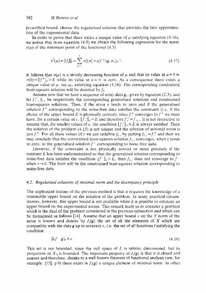
prescribed bound, choose the regularised solution that provides the best approxima- tion of the experimental data.

In order to prove that there exists a unique value of p satisfying equation (4.16), we notice that from equation (4.9) we obtain the following expression for the norm vh) of the minimum point of the functional (4.5)

(4.17)

It follows that Y@) is a strictly decreasing function of p and that its value at ,U = 0 is ~ ( 0 ) = lif'lix> E while its value at p = is zero. As a consequence there exists a unique value of p, say po, satisfying equation (4.16). The corresponding constrained least-squares solution will be denoted by f i , .

Assume now that we have a sequence of noisy datag, , given by equation (2.3), and let f: , fi,, be respectively the corresponding generalised solutions and constrained least-squares solutions. Then, if the error E tends to zero and if the generalised solution f' corresponding to the noise-free data satisfies the constraint (i.e. if the choice of the upper bound E is physically correct), sincef: converges t o f t we must have, for a certain value of E , Ilf:llx= E and thereforef: = f , , . t . It is not restrictive to assume that, for smaller values of E , the condition llf:lixs E is always satisfied. Then the solution of the problem (4.15) is not unique and the solution of minimal norm is just f : . For all these values of E we can redefinef,,,, by puttingf,,,, =f : and then we may conclude that the constrained least-squares solution f o , I converges, when E tends to zero, to the generalised solution f ' corresponding to noise-free data.

However, if the constraint is not physically correct or more precisely if the constant E has been underestimated so that the generalised solution corresponding to noise-free data satisfies the condition i i f+i lx> E , then A, , , does not converge to f' when E-+ 0. The limit will be the constrained least-squares solution corresponding to noise-free data.

4.2. Regularised solutions of minimal norm and the discrepancy principle

The unpleasant feature of the previous method is that it requires the knowledge of a reasonable upper bound on the solution of the problem. In many practical circum- stances, however, this upper bound is not available while it is possible to estimate an upper bound on the experimental errors. This remark leads us to consider a problem which is the dual of the problem considered in the previous subsection and which can be formulated as follows [14]. Assume that an upper bound E on the Y norm of the error is known and denote by J,(g) the set of all the elements of X which are compatible with the data g up to accuracy E , i.e. the set of all functions f satisfying the condition

This set is not bounded, since the null space of L is infinite dimensional, but its projection on X N is bounded. The important property of J , ( g ) is that it is closed and convex and therefore, thanks to a well known theorem of functional analysis (see, for example, [ lS ] , p 9) there exists in J,(g) a unique element of minimal norm. In other

Lineur inverse problems with discrete data: I 1 583

words, the problem

I/ f [ I x = minimum IILf - gll+ E (4.19)

which is just the dual of problem (4.15), has always a unique solution. This solution is not the null element of X , provided that the data vector satisfies the condition lIgllv> E .

This inequality is quite reasonable, since it means that the data are greater than the noise. If i t is not satisfied, the data contain only noise and therefore they do not contain any information about f . In such a case the solution of problem (4.19) is just

In order to obtain explicitly the unique solution of problem (4.19) when I l g l l y > ~ , let us first observe that the solution must necessarily belong to X , since it is a solution of minimal norm (the component belonging to the null space of L must be zero). Then it is quite easy to see that the solution of minimal norm must lie on the boundary of the bounded set which is the intersection of X N with J , ( g ) . As a consequence, the solution we are looking for satisfies the condition IILf-glly= E and one can use the method of Lagrange multipliers for determining the solution of problem (4.19). Again we must minimise the functional (4.5) for anyp and then look for a minimum pointJ, satisfying the condition

f = 0.

Thanks to the previous remarks we already know that there must exist a unique value of ,U allowing (4.20) to be satisfied. It is useful, however, to check directly this result.

From the representation (4.9) of the regularised solution f i ,, we obtain

(4.21)

and this is a strictly increasing function of ,U, which is zero at p = 0 and tends to Ikll: when ,U+ cc. Therefore, when the condition Ilglly>E is satisfied, there exists a unique value of p , say p l , which solves equation (4.20). The corresponding regularised solution will be denoted by f , .

I f we consider now the case of a sequence of noisy data g, , i t is obvious that, when the error E tends to zero, the corresponding value of the regularisation parameter p , =,U,(&) also tends to zero. As a consequence, the sequence of regularised solutions, f , ,, obtained by means of this method always converges to the generalised solution corresponding to noise-free data.

The method considered in this subsection is a particular case of a general method for the choice of the regularisation parameter which is known as the discrepancy principle [16]. The function p@), defined by (4.21) and representing the norm of the difference between the measured data and the data which can be computed from the regularised function J,, is usually called the discrepancy function.

4.3. Regularised solutions satisfying prescribed bounds

The method of $ 4.1 requires a prescribed bound on the solution while the method of $4.2 requires a prescribed bound on the data error. In a paper by Miller [17], the case where both bounds are known is also considered. Let us assume that two constants E ,

5 84 M Bertero et a1

E are given and that one looks for a function f such that

I l L f - g I l Y ~ E llf I I X ~ E . (4.22)

Any function satisfying these conditions can be called an admissible solution of the problem. Therefore the conditions (4.22) define a set K of admissible solutions and the first problem is to find a condition ensuring that this set is not empty.

For this purpose we introduce the functional

@ [ f l =IILf-gll$+ (W21Ifll~, (4.23)

which is just the functional (4.5) with p = (&/E)?, and we consider the set K , , which is the set of all the functions f satisfying the condition

@[ f] s E 2 . (4.24)

Since any function satisfying this condition also satisfies the conditions (4.22), we have the inclusion K o c K and the set K is not empty if K O is not empty. This is true if and only if @[ f2] SE’ , wheref, is the function which minimises the functional (4.23) and is given by equation (4.9) with ,u = ( E / € ) ? . In such a case f 2 E K . It follows that the regularised solution corresponding to this choice of the regularisation parameter is an admissible solution in the sense specified above.

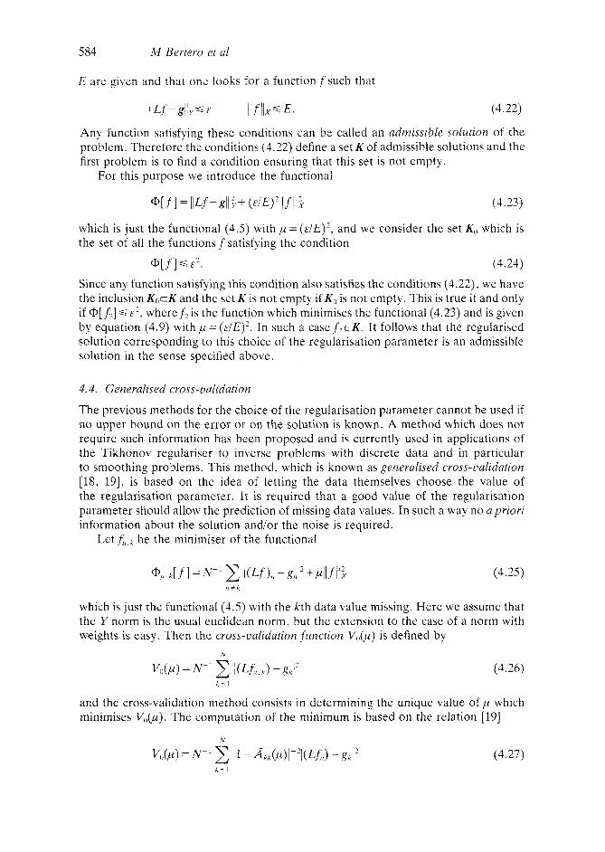
4.4. Generalised cross-validation

The previous methods for the choice of the regularisation parameter cannot be used if no upper bound on the error or on the solution is known. A method which does not require such information has been proposed and is currently used in applications of the Tikhonov regulariser to inverse problems with discrete data and in particular to smoothing problems. This method, which is known as generalised cross-validation [18, 191, is based on the idea of letting the data themselves choose the value of the regularisation parameter. It is required that a good value of the regularisation parameter should allow the prediction of missing data values. In such a way no a priori information about the solution and/or the noise is required.

Let fi, h be the minimiser of the functional

(4.25)

which is just the functional (4.5) with the kth data value missing. Here we assume that the Y norm is the usual euclidean norm, but the extension to the case of a norm with weights is easy. Then the cross-validation funct ion V,,(p) is defined by

Y

(4.26) h = I

and the cross-validation method consists in determining the unique value of p which minimises Vo(p). The computation of the minimum is based on the relation [ 191

V

k = l

(4.27)

Linear inverse problems with discrete data: I1 585

where is the minimiser of the functional N

@ , u [ f I = N - ' 2 I(~f)H-g,l12+iUI/fl/:: (4.28)

which is a special case of the functional (4.5), and AAA&) is the kk entry of the N x N matrix

[A@)] = [LL*][LL* +pur]-*. (4.29)

Notice that [LL:'] is essentially the Gram matrix of the functions q ~ ! , since, in this formulation, [W] =N-'[Z].

It has been shown [19] that, from the point of view of minimising the predictive mean-square error, the minimisation of V,@) must be replaced by the minimisation of the generalised cross-validation funct ion defined by

n = I

V(P) = w1 Tr[ l - A(P) l ) - * (~ - ' I l [~ - A(P)lgllz) (4.30)

where 11 ( 1 denotes the usual euclidean norm. A n important property of Vcu) is its invariance with respect to permutations, and more generally with respect to rotations, of the data values.

The determination of the value of ,U which minimises Vcu) might seem a quite heavy computational problem. However very efficient and fast algorithms have been developed for the solution of this problem [19].

5. Iterative methods

It is known that several iterative methods, such as successive approximations [20, 211, steepest descent [22] and conjugate gradient [23], define regularising algorithms, in the sense of Tikhonov [ 3 ] , for the approximate solution of ill-posed linear operator equations. These methods can be applied, in particular, t o the solution of first kind Fredholm integral equations. Their formulation in the present case is rather natural, since they are methods for computing the minimum of the quadratic form IILf-gliy. The Euler equation associated with this minimum problem is

(5.1) L:,:Lf = L'kg

When the functions q ~ , ~ are linearly independent, the minimum value of the functional IILf-gll, is zero and the normal solution of equation (5.1) coincides with the normal solution of equation (1.4).

Since the operator L " L is a finite rank operator in X , the iterative methods mentioned above converge to the normal solution of equation (5.1) for any data vector g , provided that the initial function of the iterative scheme is properly chosen. Equation ( 5 . l) , however, is a functional equation and it is convenient to transform it into an equivalent matrix equation. W e give here the basic formulae for the three methods.

IfJI denotes the approximation of the normal solutionf' provided by the nth step of the iteration scheme and if r,, denotes the residual

586 M Bertero et ai

then we put f = L>’:f,,,

r,, = L :’ r,,

t i

and also

r,, = GI - g

(5 .3 )

(5.4)

wheref,, and r,, are N-dimensional vectors. As in I , L = LL” and in the case where Y is the usual euclidean space, f is the Gram matrix of the functions q,,.

The algorithms mentioned above can now be formulated as follows.

5.1. Successive approximations

&I = 0 f, l+ 1 =A, - rrt, ( 5 . 5 )

0 < t < 2/a:. (5.6)

where t, the relaxation parameter, can be any number satisfying the conditions

5.2. Steepest descent

5.3. Conjugate gradient

(5.9)

(5.10)

(5.11)

0,)- I = - (L2r,,, P,,- I) Y / ( h - 1 3 P,z- J Y . (5.12)

It is not difficult to show that these three iterative algorithms have the following

(i”) the nth approximationf,,, given by equation (5.3), belongs to X , and converges properties:

to f+ when n-+ CO ; furthermore the following inequalities hold true

Linear inverse problems with discrete data: I I 587

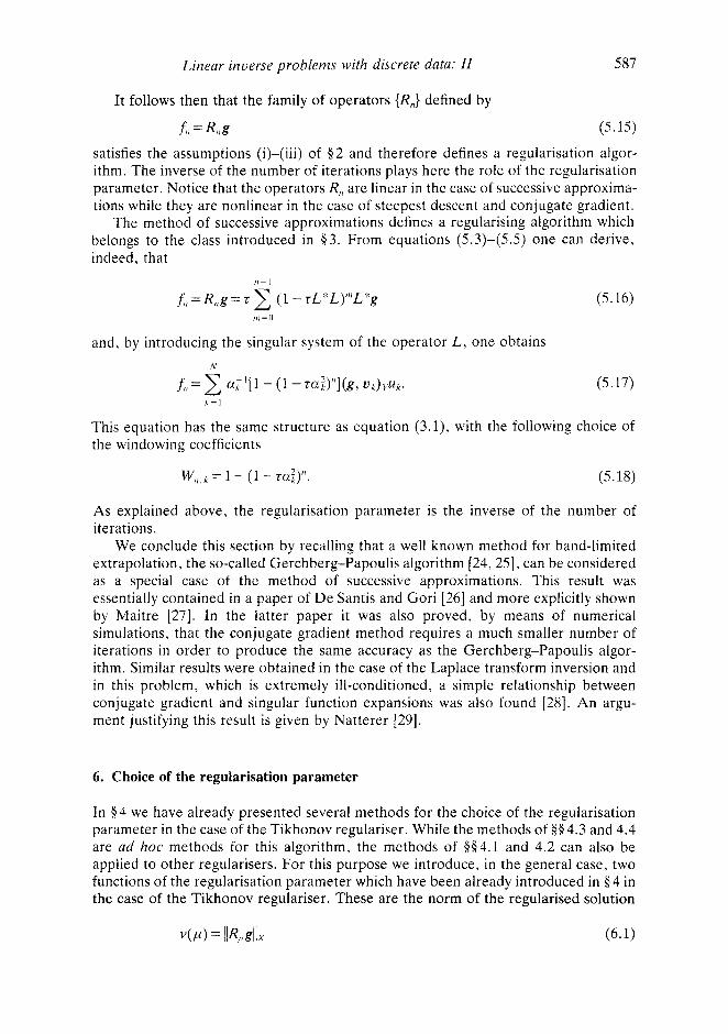
It follows then that the family of operators {R,} defined by

f i , = R,,g (5.15)

satisfies the assumptions (i)-(iii) of 02 and therefore defines a regularisation algor- ithm. The inverse of the number of iterations plays here the role of the regularisation parameter. Notice that the operators RI, are linear in the case of successive approxima- tions while they are nonlinear in the case of steepest descent and conjugate gradient.

The method of successive approximations defines a regularising algorithm which belongs to the class introduced in 63. From equations (5.3)-(5.5) one can derive, indeed, that

11- I

fil = R,,g = z (1 - tL:* L)'"L"g 111=0

and, by introducing the singular system of the operator L , one obtains N

f,,=C K ' [ I - ( ~ - ~ a ? > ' ~ ] ( g , D J Y U ~ . i = I

(5.16)

(5.17)

This equation has the same structure as equation (3.1), with the following choice of the windowing coefficients

W,!, A = 1 - (1 - taf)". (5.18)

As explained above, the regularisation parameter is the inverse of the number of iterations.

We conclude this section by recalling that a well known method for band-limited extrapolation, the so-called Gerchberg-Papoulis algorithm [24,25], can be considered as a special case of the method of successive approximations. This result was essentially contained in a paper of De Santis and Gori [26] and more explicitly shown by Maitre [27]. In the latter paper it was also proved, by means of numerical simulations, that the conjugate gradient method requires a much smaller number of iterations in order to produce the same accuracy as the Gerchberg-Papoulis algor- ithm. Similar results were obtained in the case of the Laplace transform inversion and in this problem, which is extremely ill-conditioned, a simple relationship between conjugate gradient and singular function expansions was also found [28]. An argu- ment justifying this result is given by Natterer [29].

6. Choice of the regularisation parameter

In $ 4 we have already presented several methods for the choice of the regularisation parameter in the case of the Tikhonov regulariser. While the methods of 604.3 and 4.4 are ad hoc methods for this algorithm, the methods of 004.1 and 4.2 can also be applied to other regularisers. For this purpose we introduce, in the general case, two functions of the regularisation parameter which have been already introduced in 04 in the case of the Tikhonov regulariser. These are the norm of the regularised solution

588 M Bertero et a1

and the discrepancy function

P ( P ) = Ilm3 3 I Y . (6 .2)

We will a s u m e that these functions satisfy the following conditions (a) I@) is a strictly decreasing function of p ; its value at ,U = 0 is determined by the

condition (iii) of $2 , i.e. v(O) = ~ ~ f * ~ ~ x ; (b) p ( p ) is a strictly increasing function of p ; its value at ~i = 0 is determined again

by the condition (iii) of $2 , i.e. p(0) = 0. These conditions are satisfied by the Tikhonov regulariser, by the examples of regularisers given in 43 and by the iterative algorithms of $ 5 .

Let us assume, as in $4.1, that , on the basis of physical considerations, we know an upper bound on the norm of the unknown solution f

Ilf L S E . (6 .3)

If the prescribed constant E is smaller than the norm of the generalised solution f', then it follows from property (a) that there exists a unique value of p , saypE, such that v( ,uL) = E and, f o r p >kil: , ( U ) < E . Furthermore property (b) implies that , for ,U >,L(/, we have p({u)>p(,u,). W e conclude that p=,uLy. is the value of the regularisation parameter which gives an approximate solution compatible with the constraint (6.3) and minimises the discrepancy between the computed and the measured data.

O n the other hand, let us now assume, as in $ 4.2, that the unknown function f satisfies the inequality

I l~ f -S l lYS E . (6.4)

If the prescribed constant E is smaller than the norm of g , then property (b) implies that there exists a unique value of y , say ,ut. such that p(,ul) = E and p@) < E for y <,ut. O n the other hand, it follows from property (a) that , for ,U <,U; , we have ~ ( p ) > ~ ( p , ) and therefore the va luep = k i t provides a regularised solution which is compatible with the data up to accuracy E and has minimal norm. This second method, as already mentioned in $ 4.2, is usually called the discrepurzcy principle. In the case of ill-posed problems it has been shown [30] that this principle (more precisely a slightly modified form of it. which we d o not need to mention here), when applied to the most important regularisation algorithms, always provides a regularised solution which converges to the true generalised solution of the problem as the errors on the data tend to zero. In the case of problems with discrete data, this result is almost obvious since property (b) implies then that p - 0 when E-0.

We conclude this section by mentioning a method which applies t o the case o f the truncated singular function expansions given by (3.1) and (3 .3 ) , and is the analogue of the method discussed in $4 .3 . Assume that the unknown solution satisfies the constraints (4.22). Then , as shown by Miller [17], if we keep in the expansion (1.6) only those terms which correspond to singular values fulfilling the condition

ai, 2 EIE (6 .5 )

the resulting truncated expansion satisfies the constraints (4.22) except for a factor of v2. Notice that the quantity controlling the truncation of the expansion is a kind of signal-to-noise ratio and therefore we have here an extension of the usual method of numerical filtering [ 5 ] .

Linear inverse problems with discrete data: I I 589

The result mentioned above has also an interesting interpretation from the point of view of information theory [7, 81 since it provides a generalisation of the concept of the 'information content' of a band-limited signal as introduced by Shannon. The number of singular values satisfying condition (6.5) is a generalisation of the Shannon number and, using a term introduced in optics, can be called the number of degrees of freedom (NDF) of the problem (corresponding to the given signal-to-noise ratio). The NDF is a measure of the number of independent pieces of information which can be extracted from the data and is a useful measure of information in many inversion problems, including image processing.

Let us mention that there are still many other methods for choosing the regularisa- tion parameter, which have been proposed in the literature. Reviewing them all and comparing their performances in practical inversions is beyond the scope of this paper.

7. Regularisation of C-generalised solutions

In this section we investigate the regularisation of C-generalised solutions, i.e. of solutions which minimise a seminorm instead of a norm. Since this type of solution was only shortly discussed in I , we first reconsider the problem in more detail. We analyse then the generalisation of the Tikhonov regulariser to the case of C-generalised solutions and finally we discuss a few examples.

Assume again, for simplicity. that the functions q,2 are linearly independent so that the range of the operator L , defined by equation (1.3). is the whole space Y. Moreover, let C be an operator from the Hilbert space X into the Hilbert space 2 (the constraint space) satisfying the following conditions, already stated in I :

( i ) C:X-+Z is a linear closed operator, with domain %(C) dense in X and %(C) closed in 2;

(ii) the null space X(C) of C is nontrivial but x ' ( L ) n A"(C) ={U}, i.e. the unique solution of the problem

Lf=O Cf = 0 (7.1) is f = O . Then the C-generalised solution, f ; , is the solution of equation (1.4) which minimises the functional (4.3). Notice that, since JC'(C) is nontrivial, the functional p ( f ) = IICf/l,. is not a norm but a seminorm.

As stated in I , under the previous conditions on the constraint operator C, there exists a unique C-generalised solution for any g E Y . By applying to our special case a method developed in a more general framework [31] it is possible to characterisef,+ as the generalised solution of a modified problem.

The product operator { L , C}:X-+ Y@Z, with domain %(C), is linear, closed and invertible. Moreover its range is Y@%(C) and hence it is closed in Y@Z. It follows that the inverse operator is continuous and this implies that there exists a constant p > 0 such that

l l Lf llzy + I1 Cf 11: 2= PI1 f Ilb (7.2) for anyfE%(C). By means of this inequality it is easy to show that %m(C), endowed with the scalar product

( f , A), ,= (Lf, LA),+ (Cf, Ch):, (7.3)

590 M Bertero et a1

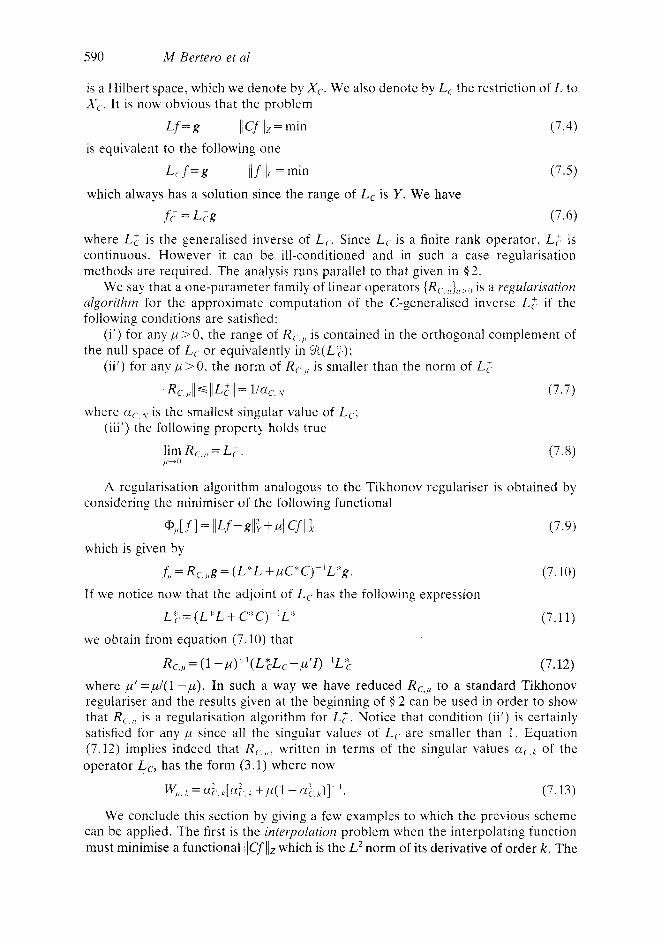
is a Hilbert space. which we denote by X,. We also denote by L, the restriction of L to X , . It is now obvious that the problem

L f = g lICfll2 = min (7.4) is equivalent to the following one

L,.f = g l l f /I, = min (7.5) which always has a solution since the range of Lc is Y . W e have

f; = L;g (7.6)

where L,+ is the generalised inverse of L,.. Since L,- is a finite rank operator, L; is continuous. However it can be ill-conditioned and in such a case regularisation methods are required. The analysis runs parallel to that given in $2.

is a regularisation algorithm for the approximate computation of the C-generalised inverse L; if the following conditions are satisfied:

( i f ) for any p > O , the range of R(.,,, is contained in the orthogonal complement of the null space of L,. or equivalently in Yt(L:l.);

(ii') for any p > 0, the norm of R,.,l, is smaller than the norm of L ,

W e say that a one-parameter family of linear operators { R ,

IIRC. ,,I1 llL;ll = 1/ac, L' (7.7) where ac, ,y is the smallest singular value of Lc;

(iii') the following property holds true

A regularisation algorithm analogous to the Tikhonov regulariser is obtained by considering the minimiser of the following functional

@,I [ f I = I1 Lf - gll$ + PI1 Cf lib

j', = R, . . , ,g= (L: 'L +pC"c)-'L'Kg,

L:;,=(L:kL + c:i;

(7.9)

(7.10)

which is given by

If we notice now that the adjoint of L,, has the following expression

C) - ' L :K (7.11)

we obtain from equation (7.10) that

RC+ = (1 -p)-'(L*cLc+p'z)-'L*c (7.12) where p' =pU/(l - , U ) . In such a way we have reduced Rc,p to a standard Tikhonov regulariser and the results given at the beginning of $ 2 can be used in order to show that RC,,, is a regularisation algorithm for LT. Notice that condition (ii') is certainly satisfied for any p since all the singular values of L(. are smaller than 1. Equation (7.12) implies indeed that R,.,,,, written in terms of the singular values of the operator Lc, has the form (3.1) where now

w,,,, = at..h[a:.,k +pi1 - a ; , L ) ] - ' . (7.13)

W e conclude this section by giving a few examples to which the previous scheme can be applied. The first is the interpolation problem when the interpolating function must minimise a functional llCfliz which is the L2 norm of its derivative of order k . The

Lineur inverse problems with discrete data: I1 591

corresponding C-generalised solution is a natural spline of degree m = 2k - 1. Then the regularised solution provided by equation (7.10) is just the solution of the smoothing problem investigated by Reinsch [32] and is again a spline function. The choice of the regularisation parameter is based on the method that we have called the discrepancy principle.

The second example is the method of Phillips [12] for the solution of first-kind Fredholm integral equations and in such a case the functional liCfl17 is the L’ norm of the second derivative of the unknown function. In that paper only regularised solutions are considered and again the discrepancy principle is used for the choice of the regularisation parameter.

The scheme presented in this section also applies to a recent investigation of the moment problem [33] where the constraint was the L’ norm of the first derivative of the solution. A stability theorem was also proved in this paper and the dependence of the solution on the number of moments was quantified for a given noise level.

8. The Backus-Gilbert method

As shown in 0 2, in the case where X is a space of square integrable functions, any regularised solution can be written, in the absence of noise, as an average of the true solution f

the averaging kernel A(x, x‘) being given, in general, by equation (2.12). The same remark applies as well to the generalised solution-see I.

The relation (8.1) is the starting point of the Backus-Gilbert method [34, 351 which applies to the case where X is a space of square integrable functions. As in equation (2.12), it is assumed that the averaging kernel A(x, x’) is a linear combi- nation of the functions q : ( x ’ )

N

A ( x , x’) = a , l ( x ) q W ) (8.2) ll= I

but the coefficients a,,(x) are not assumed to be linear combinations of the functions q&). They are determined by introducing a variational principle for the averaging kernel, namely by requiring that they give the sharpest averaging kernel in a sense to be specified. For this purpose Backus and Gilbert introduce a function J(x, x’) which vanishes when x = x’ and increases monotonically as x goes away from x’. An example of such a function is

J(x, x’) = (x - X I ) ? . ( 8 . 3 ) Then the averaging kernel is determined by solving, for any x in the domain of the unknown function f ( x ) , the following constrained minimisation problem

8(x) = J(x, x’) lA(x , x’)l’ du’ = min I A ( x , x’) du’ = 1. I

592 M Bertero et a1

I f we introduce the quantities

S, , , , , (x ) = J(x. x‘)y7),(x‘)y7;;,(xr) dx’ (8.6) I h, = U?,,(x) dx I then we find that d2(x) is a quadratic functional of the functions ail(x) and that the problem (8.4)-(8.5) is a standard minimisation problem

,I’

~’(x) = s,,,,,(x)a,,,(x>u~~(x) = min (8.7) , l L , l l ~ l

, , = I

which can be solved by means of the method of Lagrange multipliers. If for any x the matrix [S(x)] is nonsingular and if we denote by S’”’(x) the elements of the inverse matrix, then the solution of the previous problem is

1

ql(x) = L(x) S“”’(x)b,,, I l l = I

the Lagrange multiplier L ( x ) being given by

(8.10) /

Using equation (1.1) we find that the solution provided by the Backus-Gilbert method is

N

(8.11) i n= 1 i n = l

.N

~ B G ( x ) = ~(x,x‘)f(x’) kf =C an(x> ~(x’)v;(x’) &’=E gnan(x>

and therefore it belongs to the subspace spanned by the functions an(x). This solution is a type of generalised solution even if it is different fromf’(x) since it belongs to the subspace spanned by the functions a,,(x) while f + belongs to the subspace spanned by the functions q , ? ( x ) . It is also obvious that the functions aJi(x) depend on the function J(x, x’) which has been chosen for characterising the sharpness of the averaging kernel. As already remarked by Backus and Gilbert, their solution can also be affected by numerical instability. In order to overcome this difficulty they proceed as follows [35] .

If the covariance matrix [C] of the noise is known, then from equation (8.11) one easily derives that, at any given point x, the variance of the error induced by the noise onfnG(x) is

1‘

&) = c c , , ! , l a , , , ( ~ ) m ) . (8.12) ,,. / , z = I

Then Backus and Gilbert consider two methods:

d’(x) SE’, which prescribes an upper limit on the desired resolution distance; (1) minimise the functional 02(x) with the constraint (8.8) and also the constraint

Lineur iriuerse problems with discrete datu: I I 593

(2) minimise the functional B’(x) with the constraint (8.8) and also the constraint o’(x) 6 E’, which prescribes an upper limit on the error affecting the reconstructed solution.

Both problems can be solved again by means of the method of Lagrange multipliers and we do not give the details here. Let us just remark that these two methods are similar to the methods described respectively in SS4.1 and 4.2 for the case of the Tikhonov regulariser. They amount in fact to a form of regularisation of the Backus-Gilbert solution. Applications of these methods and numerical algorithms for implementing them have been considered by several authors [36-381. In the case where the functionals are the Fourier coefficients off(x) as given by equation (3.5), a similarity between the Backus-Gilbert method and the Fejer method has also been noticed [39].

Acknowledgments

This research has been partly supported by NATO Grant No 463184 and EEC Contract No ST29-0089-3. C De Mol is ‘Chercheur qualifi6’ with the Belgian National Fupd for Scientific Research (FNRS).

References

[I] Bertero M, De Mol C and Pike E R 1985 Linear inverse problems with discrete data. I: General

[2] Lavrentiev M M 1967 Some Improperly Posed Problems of Muthc.muiical Physics (Berlin: Springer) 131 Tikhonov A N and Arsen,ine V Y 1977 Solutions of /ll-Po.sed Problems (Washington, DC:

141 Groetsch C W 1984 The Theory of Tikhonoo Regulnrizuiiori for Fredholm Equutior7.s of the First Kind

[5] Twomey S 1985 The application of numerical filtering to the solution of integral equations encountered

[6] Twomey S 1974 Information content in remote sensing Appl. Opi. 13 942-5 171 Bertero M and De Mol C 1981 Ill-posedness. regularization and number of degrees of freedom Arii

[SI Pike E R , McWhirter J G. Bertero M and De Mol C 1984 Generalised information theory for inverse prohlems in signal processing l E E E Proc. 131 660-7

[9] Titchmarsh E C 1948 lntroduciiori io the Theory of’ Fourier lnregrds (London: Oxford University Press)

[IO] Bcrtero M. Brianzi P. De Mol C and Pike E R 1986 Positive regularized solutions in electromagnetic inverse scattering Proc. URSI Int. Symp. on Electromagnetic Theory, Budapest Part A (Budapest: Akademiai Kiado) pp 150-2

[ l l ] Tikhonov A N 1963 Solution of incorrectly formulated problems and the regularization method Sou. Phys.-Math. Dokl. 4 1035

[12] Phillips D L 1962 A technique for the numerical solution of certain integral equations of the first kind J . Assn Comput. Mach. 9 84

[13] Ivanov V K 1962 O n linear problems which are not well-posed Sou. Phys.-Math. Dokl. 3 981 [ 141 Ivanov V K 1966 The approximate solution of operator equations of the first kind USSR Comp. Mnih.

[ IS] Balakrishnan A V 1976 Applied Firnciionul Amlysis (Berlin: Springer) [16] Morozov V A 1968 The error principle in the solution of operational equations by the regularization

1171 Miller K 1970 Least squares methods for ill-posed problems with a prescribed bound S l A M J . Math.

[ I X ] Golub G H. Heath M and Wahba G 1979 Generalized cross-validation as a method for choosing a

formulation and singular system analysis lnuerse Problems 1 301-30

Winston/Wiley)

(Research Notes in Mathematics vol. 105) (Boston: Pitman)

in indirect sensing measurements J . Franklin Inst. 279 95-109

Fotld. G . Rot?chi 36 619-32

Mtirh. Phj’.s. 6 6 197

method USSR Comp. Math. Math. Phys. 8 2 63

Anal. IS2

good ridge parameter Technometrics 21 215

594 M Bertero et nl

[ 191 Craven P and Wahha G 1979 Smoothing noisy data with spline functions: estimating the correct degree

[ZO] Landweher L 1951 An iteration formula for Fredholm integral equations of the first kind Am. J . Math .

[21] Bialy H 1959 Iterative behandlung linearer funktionalgleichungen Arch. Rat. Mech. Anal 4 166 1221 Kammerer W J and Nashed M Z 1971 Steepest deacent f o r singular linear operators with nonclosed

1231 Kammerer W J and Nashed M 2 1972 On the convergence of the conjugate gradient method for

1241 Gerchberg R W 1974 Super-rcsolution through error energy reduction Opt . Actu 21 709 1251 Papotilia A 1975 A new algorithm in spectral analysis and band-limited extrapolation IEEE Truns.

[26] De Santis P and Gori F 1975 On an iterative method for super-resolution O p t . Ac tu 22 691 [27] Maitre H 1981 Iterative superresolution. Some new fast methods Opt. Acta 28 973 [28] Bertero M, Brianzi P , Defrise M and D e Mol C 1986 Iterative inversion of experimental data in

[29] Natterer F 1986 Numerical treatment of ill-posed problems Ini1err.e Problems (ed. G Talenti) (Lect.

[30] Vainikko G M 1982 The discrepancy principle for a class o f regularization methods U S S R Camp.

[31] Groetsch C W 1986 Regularization with linear equality constraints 1t711erse Problems (ed. G Talenti)

[32] Reinsch C H 1Y67 Smoothing by spline functions Nutnrr . Math . 10 177 [33] Talenti G 1987 Recovering a function from a finite number of moments Inoerse Prohlems 3 501 1341 Backus G and Gilbert F 1968 The resolving power of gross Earth data Geophys. J . R . Astroti . Soc. 16

[35] Backus G and Gilbert F 1970 Uniqueness in the inversion of inaccurate gross Earth data Phil. Truti.s.

[36] Oldenburg D W 1976 Calculation of Fourier transforms by the Backus-Gilbert method GeophyA. J . R .

[37] Colton D 1984 The inverse scattering problem for time-harmonic acoustic waves S I A M Reo. 26 323 [38] Haario H and Somersalo E 1985 On the numerical implementation of the Backus-Gilbert method

I391 Bertero M, Brianzi P, Pike E R and Rebolia L 1988 Linear regularizing algorithms for positive

of smoothing by the method of generalized cross-validation N u m . Moth. 31 377

73 615

range Applicable A n d . 1 143

singular linear operator equations S I A M J . Numer. Anal. 9 I65

. Circuits Syst. CAS-22 735

weighted spaces Proc. URSI Int. Symp. on Electromagnetic Theory, Budapest Part A p 315

Notes in Math.. vol 1225) (Berlin: Springer)

Math. Math . Phys . 22 3 1

(Lect. Notes in Math., vol 1225) (Berlin: Springer)

169

R . Soc. 266 123

Astroti . Soc. 44 413

Cahiers Muth . de Motitpellier 32 107

solutions of linear inverse problems Proc. R. Soc. A 415 257-75