computational learning theory - citeseerx
TRANSCRIPT
Computational Learning Theory
Lecture Notes for CS 582
Spring Semester, 1991
Sally A. Goldman
Department of Computer Science
Washington University
St. Louis, Missouri 63130
WUCS-91-36
1
Preface
This manuscript is a compliation of lecture notes from the graduate level course CS 582,\Computational Learning Theory," I taught at Washington University in the spring of 1991.
Students taking the course were assumed to have background in the design and analysis ofalgorithms as well as good mathematical background. Given that there is no text availableon this subject, the course material was drawn from recent research papers. I selected the�rst twelve topics and the remainder were selected by the students from a list of providedtopics. This list of topics is given at the end of these notes.
These notes were mostly written by the students in the class and then reviewed by
me. However, there are likely to be errors and omissions, particularly with regard to thereferences. Readers �nding errors in the notes are encouraged to notify me by electronicmail ([email protected]) so that later versions may be corrected.

2
3
Acknowledgements
This compilation of notes would not have been possible without the hard work of thefollowing students: Andy Fingerhut, Nilesh Jain, Gadi Pinkas, Kevin Ruland, Marc Wallace,
Ellen Witte, and Weilan Wu.I thank Mike Kearns and Umesh Vazirani for providing me with a draft of the scribe
notes from their Computational Learning Theory course taught at University of Californiaat Berkeley in the Fall of 1990. Some of my lectures were prepared using their notes. Alsomost of the homework problems which I gave came from the problems used by Ron Rivestfor his Machine Learning course at MIT taught during the Falls of 1989 and 1990. I thank
Ron for allowing me to include these problems here.

4
Contents
Introduction 9
1.1 Course Overview : : : : : : : : : : : : : : : : : : : : : : : : : : : : : : : : : 9
1.2 Introduction : : : : : : : : : : : : : : : : : : : : : : : : : : : : : : : : : : : : 10
1.2.1 A Research Methodology : : : : : : : : : : : : : : : : : : : : : : : : : 10
1.2.2 De�nitions : : : : : : : : : : : : : : : : : : : : : : : : : : : : : : : : : 11
1.3 The Distribution-Free (PAC) Model : : : : : : : : : : : : : : : : : : : : : : : 121.4 Learning Monomials in the PAC Model : : : : : : : : : : : : : : : : : : : : : 13
1.5 Learning k-CNF and k-DNF : : : : : : : : : : : : : : : : : : : : : : : : : : : 15
Two-Button PAC Model 17
2.1 Model De�nition : : : : : : : : : : : : : : : : : : : : : : : : : : : : : : : : : 17
2.2 Equivalence of One-Button and Two-Button Models : : : : : : : : : : : : : : 17
Aside: Cherno� Bounds : : : : : : : : : : : : : : : : : : : : : : : : : : : : : 19
Learning k-term-DNF 23
3.1 Introduction : : : : : : : : : : : : : : : : : : : : : : : : : : : : : : : : : : : : 233.2 Representation-dependent Hardness Results : : : : : : : : : : : : : : : : : : 23
3.3 Learning Algorithm for k-term-DNF : : : : : : : : : : : : : : : : : : : : : : 26
3.4 Relations Between Concept Classes : : : : : : : : : : : : : : : : : : : : : : : 27
Handling an Unknown Size Parameter 29
4.1 Introduction : : : : : : : : : : : : : : : : : : : : : : : : : : : : : : : : : : : : 29
4.2 The Learning Algorithm : : : : : : : : : : : : : : : : : : : : : : : : : : : : : 29
Aside: Hypothesis Testing : : : : : : : : : : : : : : : : : : : : : : : : : : : : 29
Learning With Noise 33
5.1 Introduction : : : : : : : : : : : : : : : : : : : : : : : : : : : : : : : : : : : : 33
5.2 Learning Despite Classi�cation Noise : : : : : : : : : : : : : : : : : : : : : : 35
5.2.1 The Method of Minimizing Disagreements : : : : : : : : : : : : : : : 35
5.2.2 Handling Unknown �b : : : : : : : : : : : : : : : : : : : : : : : : : : 37
5.2.3 How Hard is Minimizing Disagreements? : : : : : : : : : : : : : : : : 375.3 Learning k-CNF Under Random Misclassi�cation Noise : : : : : : : : : : : : 38
5.3.1 Basic Approach : : : : : : : : : : : : : : : : : : : : : : : : : : : : : : 38
5
6 CONTENTS
5.3.2 Details of the Algorithm : : : : : : : : : : : : : : : : : : : : : : : : : 41
Occam's Razor 43
6.1 Introduction : : : : : : : : : : : : : : : : : : : : : : : : : : : : : : : : : : : : 43
6.2 Using the Razor : : : : : : : : : : : : : : : : : : : : : : : : : : : : : : : : : : 43
The Vapnik-Chervonenkis Dimension 47
7.1 Introduction : : : : : : : : : : : : : : : : : : : : : : : : : : : : : : : : : : : : 47
7.2 VC Dimension De�ned : : : : : : : : : : : : : : : : : : : : : : : : : : : : : : 47
7.3 Example Computations of VC Dimension : : : : : : : : : : : : : : : : : : : : 48
7.4 VC Dimension and Sample Complexity : : : : : : : : : : : : : : : : : : : : : 51
7.5 Some Relations on the VC Dimension : : : : : : : : : : : : : : : : : : : : : : 54
Representation Independent Hardness Results 57
8.1 Introduction : : : : : : : : : : : : : : : : : : : : : : : : : : : : : : : : : : : : 57
8.2 Previous Work : : : : : : : : : : : : : : : : : : : : : : : : : : : : : : : : : : 57
8.3 Intuition : : : : : : : : : : : : : : : : : : : : : : : : : : : : : : : : : : : : : : 58
8.4 Prediction Preserving Reductions : : : : : : : : : : : : : : : : : : : : : : : : 59
The Strength of Weak Learnability 61
9.1 Introduction : : : : : : : : : : : : : : : : : : : : : : : : : : : : : : : : : : : : 61
9.2 Preliminaries : : : : : : : : : : : : : : : : : : : : : : : : : : : : : : : : : : : 61
9.3 The Equivalence of Strong and Weak Learning : : : : : : : : : : : : : : : : : 62
9.3.1 Hypothesis Boosting : : : : : : : : : : : : : : : : : : : : : : : : : : : 62
9.3.2 The Learning Algorithm : : : : : : : : : : : : : : : : : : : : : : : : : 64
9.3.3 Correctness : : : : : : : : : : : : : : : : : : : : : : : : : : : : : : : : 64
9.3.4 Analysis of Time and Sample Complexity : : : : : : : : : : : : : : : 67
9.4 Consequences of Equivalence : : : : : : : : : : : : : : : : : : : : : : : : : : : 68
Learning With Queries 69
10.1 Introduction : : : : : : : : : : : : : : : : : : : : : : : : : : : : : : : : : : : : 69
10.2 General Learning Algorithms : : : : : : : : : : : : : : : : : : : : : : : : : : 70
10.2.1 Exhaustive Search : : : : : : : : : : : : : : : : : : : : : : : : : : : : 70
10.2.2 The Halving Algorithm : : : : : : : : : : : : : : : : : : : : : : : : : : 70
10.3 Relationship Between Exact Identi�cation and PAC Learnability : : : : : : : 71
10.4 Examples of Exactly Identi�able Classes : : : : : : : : : : : : : : : : : : : : 72
10.4.1 k-CNF and k-DNF Formulas : : : : : : : : : : : : : : : : : : : : : : : 73
10.4.2 Monotone DNF Formulas : : : : : : : : : : : : : : : : : : : : : : : : 73
10.4.3 Other E�ciently Learnable Classes : : : : : : : : : : : : : : : : : : : 75
Learning Horn Sentences 77
11.1 Introduction : : : : : : : : : : : : : : : : : : : : : : : : : : : : : : : : : : : : 77
11.2 Preliminaries : : : : : : : : : : : : : : : : : : : : : : : : : : : : : : : : : : : 77
CONTENTS 7
11.3 The Algorithm : : : : : : : : : : : : : : : : : : : : : : : : : : : : : : : : : : 78
11.4 Example Run of Algorithm : : : : : : : : : : : : : : : : : : : : : : : : : : : : 80
11.5 Analysis of Algorithm : : : : : : : : : : : : : : : : : : : : : : : : : : : : : : 81
Learning with Abundant Irrelevant Attributes 83
12.1 Introduction : : : : : : : : : : : : : : : : : : : : : : : : : : : : : : : : : : : : 83
12.2 On-line Learning Model : : : : : : : : : : : : : : : : : : : : : : : : : : : : : 83
12.3 De�nitions and Notation : : : : : : : : : : : : : : : : : : : : : : : : : : : : : 85
12.4 Halving Algorithm : : : : : : : : : : : : : : : : : : : : : : : : : : : : : : : : 85
12.5 Standard Optimal Algorithm : : : : : : : : : : : : : : : : : : : : : : : : : : : 86
12.6 The Linear Threshold Algorithm: WINNOW1 : : : : : : : : : : : : : : : : : 88
12.7 Extensions: WINNOW2 : : : : : : : : : : : : : : : : : : : : : : : : : : : : : 91
12.8 Transformations to Other Concept Classes : : : : : : : : : : : : : : : : : : : 92
Learning Regular Sets 95
13.1 Introduction : : : : : : : : : : : : : : : : : : : : : : : : : : : : : : : : : : : : 95
13.2 The Learning Algorithm : : : : : : : : : : : : : : : : : : : : : : : : : : : : : 95
13.3 An Example : : : : : : : : : : : : : : : : : : : : : : : : : : : : : : : : : : : : 97
13.4 Algorithm Analysis : : : : : : : : : : : : : : : : : : : : : : : : : : : : : : : : 102
13.4.1 Correctness of L� : : : : : : : : : : : : : : : : : : : : : : : : : : : : : 102
13.4.2 Termination of L� : : : : : : : : : : : : : : : : : : : : : : : : : : : : : 104
13.4.3 Runtime complexity of L� : : : : : : : : : : : : : : : : : : : : : : : : 105
Results on Learnability and the VC-Dimension 107
14.1 Introduction : : : : : : : : : : : : : : : : : : : : : : : : : : : : : : : : : : : : 107
14.2 Dynamic Sampling : : : : : : : : : : : : : : : : : : : : : : : : : : : : : : : : 108
14.3 Learning Enumerable Concept Classes : : : : : : : : : : : : : : : : : : : : : 108
14.4 Learning Decomposable Concept Classes : : : : : : : : : : : : : : : : : : : : 109
14.5 Reducing the Number of Stages : : : : : : : : : : : : : : : : : : : : : : : : : 111
Learning in the Presence of Malicious Noise 113
15.1 Introduction : : : : : : : : : : : : : : : : : : : : : : : : : : : : : : : : : : : : 113
15.2 De�nitions and Notation : : : : : : : : : : : : : : : : : : : : : : : : : : : : : 113
15.3 Upper Bounds on EM(C) : : : : : : : : : : : : : : : : : : : : : : : : : : : : : 114
15.4 Generalization of Occam's Razor : : : : : : : : : : : : : : : : : : : : : : : : 116
15.5 Using Positive and Negative Examples to Improve Learning Algorithms : : : 117
15.6 Relationship between Learning Monomials with Errors and Set Cover : : : : 119
Inferring Graphs from Walks 123
16.1 Introduction : : : : : : : : : : : : : : : : : : : : : : : : : : : : : : : : : : : : 123
16.2 Intuition : : : : : : : : : : : : : : : : : : : : : : : : : : : : : : : : : : : : : : 124
16.3 Preliminaries : : : : : : : : : : : : : : : : : : : : : : : : : : : : : : : : : : : 125
16.4 Inferring Linear Chains from End-to-end Walks : : : : : : : : : : : : : : : : 127
8 CONTENTS
16.5 Inferring Linear Chains from General Walks : : : : : : : : : : : : : : : : : : 130
16.6 Inferring Cycles from Walks : : : : : : : : : : : : : : : : : : : : : : : : : : : 132
Learning in an In�nite Attribute Space 137
17.1 Introduction and Description of Model : : : : : : : : : : : : : : : : : : : : : 137
17.2 Learning Monotone Disjunctions : : : : : : : : : : : : : : : : : : : : : : : : : 138
17.3 Learning Monotone k-CNF : : : : : : : : : : : : : : : : : : : : : : : : : : : : 138
17.4 Learning Non-Monotone k-CNF : : : : : : : : : : : : : : : : : : : : : : : : : 139
17.5 Generalized Halving Algorithm : : : : : : : : : : : : : : : : : : : : : : : : : 140
17.6 Other Topics : : : : : : : : : : : : : : : : : : : : : : : : : : : : : : : : : : : 141
The Weighted Majority Algorithm 143
18.1 Introduction : : : : : : : : : : : : : : : : : : : : : : : : : : : : : : : : : : : : 143
18.2 Weighted Majority Algorithm : : : : : : : : : : : : : : : : : : : : : : : : : : 144
18.3 Analysis of Weighted Majority Algorithm : : : : : : : : : : : : : : : : : : : : 14518.4 Variations on Weighted Majority : : : : : : : : : : : : : : : : : : : : : : : : 147
18.4.1 Shifting Target : : : : : : : : : : : : : : : : : : : : : : : : : : : : : : 14718.4.2 Selection from an In�nite Pool : : : : : : : : : : : : : : : : : : : : : : 14818.4.3 Pool of Functions : : : : : : : : : : : : : : : : : : : : : : : : : : : : : 148
18.4.4 Randomized Responses : : : : : : : : : : : : : : : : : : : : : : : : : : 149
Implementing the Halving Algorithm 151
19.1 The Halving Algorithm and Approximate Counting : : : : : : : : : : : : : : 15119.2 Learning a Total Order : : : : : : : : : : : : : : : : : : : : : : : : : : : : : : 154
Choice of Topics 157
Homework Assignment 1 161
Homework Assignment 2 163
Homework Assignment 3 165
Bibliography 167
CS 582T Computational Learning Theory Spring Semester, 1991
Topic 1: Introduction
Lecturer: Sally Goldman Scribe: Ellen Witte
1.1 Course Overview
Building machines that learn from experience is an important research goal of arti�cialintelligence, and has therefore been an active area of research. Most of the work in machinelearning is empirical research. In such research, learning algorithms typically are judged bytheir performance on sample data sets. Although these ad hoc comparisons may providesome insight, it is di�cult to compare two learning algorithms carefully and rigorously, or
to understand in what situations a given algorithm might perform well, without a formallyspeci�ed learning model with which the algorithms may be evaluated.
Recently, considerable research attention has been devoted to the theoretical study ofmachine learning. In computational learning theory one de�nes formal mathematical modelsof learning that enable rigorous analysis of both the predictive power and the computationale�ciency of learning algorithms. The analysis made possible by these models provides aframework in which to design algorithms that are provably more e�cient in both their use
of time and data.
During the �rst half of this course we will cover the basic results in computational learning
theory. This portion will include a discussion of the distribution-free (or PAC) learningmodel, the model of learning with queries, and the mistake-bound (or on-line) learningmodel. The primary goal is to understand how these models relate to one another andwhat classes of concepts are e�ciently learnable in the various models. Thus we will present
e�cient algorithms for learning various concept classes under each model. (And in some
cases we will consider what can be done if the computation time is not restricted to bepolynomial.) In contrast to these positive results we present hardness results for some
concept classes indicating that no e�cient learning algorithm exists. In addition to studyingthe basic noise-free versions of these learning models, we will also discuss various models of
noise and techniques for designing algorithms that are robust against noise. Finally, during
the second half of this course we will study a selection of topics that follow up on the materialpresented during the �rst half of the course. These topics were selected by the students, and
are just a sample of the types of other results that have been obtained. We warn the readerthat this course only covers a small portion of the models, learning techniques, and methods
for proving hardness results that are currently available in the literature.
9
1.2 Introduction
In this section we give a very basic overview of the area of computational learning theory.
Portions of this introduction are taken from Chapter 2 of Goldman's thesis [18]. Also see
Chapter 2 of Kearns' thesis [27] for additional de�nitions and background material.
1.2.1 A Research Methodology
Before describing formal models of learning, it is useful to outline a research methodology
for applying the formalism of computational learning theory to \real-life" learning problems.
There are four steps to the methodology.
1. Precisely de�ne the problem, preserving key features while simplifying as much aspossible.
2. Select an appropriate formal learning model.
3. Design a learning algorithm.
4. Analyze the performance of the algorithm using the formal model.
In Step 2, selecting an appropriate formal learning model, there are a number of questionsto consider. These include:
� What is being learned?
� How does the learner interact with the environment? (e.g., Is there a helpful teacher?
An adversary?)
� What is the prior knowledge of the learner?
� How is the learner's hypothesis represented?
� What are the criteria for successful learning?
� How e�cient is the learner in time, data and space?
It is critical that the model chosen accurately re ect the real-life learning problem.
10
1.2.2 De�nitions
In this course, we consider a restricted type of learning problem called concept learning.
In a concept learning problem there are a set of instances and a single target concept that
classi�es each instance as a positive or a negative instance. The instance space denotes the
set of all instances that the learner may see. The concept space denotes the set of all concepts
from which the target concept can be chosen. The learner's goal is to devise a hypothesis of
the target concept that accurately classi�es each instance as positive or negative.
For example, one might wish to teach a child how to distinguish chairs from other furni-
ture in a room. Each item of furniture is an instance; the chairs are positive instances and
all other items are negative instances. The goal of the learner (in this case the child) is to
develop a rule for the concept of a chair. In our models of learning, one possibility is that
the rules are Boolean functions of features of the items presented, such as has-four-legs oris-wooden.
Since we want the complexity of the learning problem to depend on the \size" of the
target concept, often we assign to it some natural size measure n. If we let Xn denote theset of instances to be classi�ed for each problem of size n, we say that X =
Sn�1Xn is the
instance space, and each x 2 X is an instance. For each n � 1, we de�ne each Cn � 2Xn tobe a family of concepts over Xn, and C =
Sn�1 Cn to be a concept class over X. For c 2 Cn
and x 2 Xn, c(x) denotes the classi�cation of c on instance x. That is, c(x) = 1 if and only
if x 2 c. We say that x is a positive instance of c if c(x) = 1 and x is a negative instanceof c if c(x) = 0. Finally, a hypothesis h for Cn is a rule that given any x 2 Xn outputs inpolynomial time a prediction for c(x). The hypothesis space is the set of all hypotheses h thatthe learning algorithm may output. The hypothesis must make a prediction for each x 2 Xn.For the learning models which we will study here, it is not acceptable for the hypothesis toanswer \I don't know" for some instances.
To illustrate these de�nitions, consider the concept class of monomials. (A monomial isa conjunction of literals, where each literal is either some boolean variable or its negation.)For this concept class, n is the number of variables. Thus jXnj = 2n where each x 2 Xn
represents an assignment of 0 or 1 to each variable. Observe that each variable can beplaced in the target concept unnegated, placed in the target concept negated, or not putin the target concept at all. Thus, jCnj = 3n. One possible target concept for the class of
monomials over �ve variables is x1x4x5. For this target concept, the instance \10001" is apositive instance and \00001" is a negative instance.
We will model the learning process as consisting of two phases, a training phase and aperformance phase. In the training phase the learner is presented with labeled examples (i.e.,
an example is chosen from the instance space and labeled according to the target concept).
Based on these examples the learner must devise a hypothesis of the target concept. In
the performance phase the hypothesis is used to classify examples from the instance space,
and the accuracy of the hypothesis is evaluated. The various models of learning will di�erprimarily in the way they allow the learner to interact with the environment during the
training phase and how the hypothesis is evaluated.
11
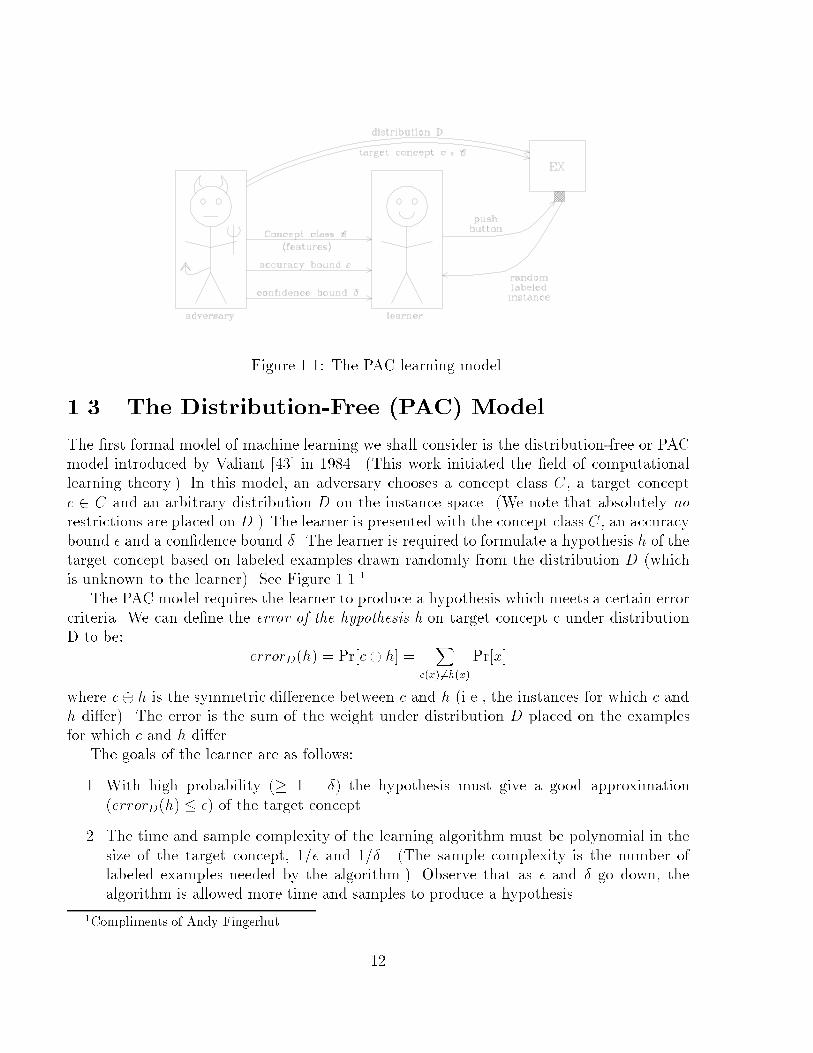
Figure 1.1: The PAC learning model.
1.3 The Distribution-Free (PAC) Model
The �rst formal model of machine learning we shall consider is the distribution-free or PACmodel introduced by Valiant [43] in 1984. (This work initiated the �eld of computationallearning theory.) In this model, an adversary chooses a concept class C, a target concept
c 2 C and an arbitrary distribution D on the instance space. (We note that absolutely norestrictions are placed on D.) The learner is presented with the concept class C, an accuracybound � and a con�dence bound �. The learner is required to formulate a hypothesis h of thetarget concept based on labeled examples drawn randomly from the distribution D (whichis unknown to the learner). See Figure 1.1.1
The PAC model requires the learner to produce a hypothesis which meets a certain errorcriteria. We can de�ne the error of the hypothesis h on target concept c under distributionD to be:
errorD(h) = Pr[c� h] =X
c(x)6=h(x)
Pr[x]
where c� h is the symmetric di�erence between c and h (i.e., the instances for which c andh di�er). The error is the sum of the weight under distribution D placed on the examplesfor which c and h di�er.
The goals of the learner are as follows:
1. With high probability (� 1 � �) the hypothesis must give a good approximation
(errorD(h) � �) of the target concept.
2. The time and sample complexity of the learning algorithm must be polynomial in the
size of the target concept, 1=� and 1=�. (The sample complexity is the number oflabeled examples needed by the algorithm.) Observe that as � and � go down, the
algorithm is allowed more time and samples to produce a hypothesis.
1Compliments of Andy Fingerhut.
12
This model is called distribution-free because the distribution on the examples is unknown
to the learner. Because the hypothesis must have high probability of being approximately
correct, it is also called the PAC model.
1.4 Learning Monomials in the PAC Model
We would like to investigate various concept classes that can be learned e�ciently in the
PAC model. The concept class of monomials is one of the simplest to learn and analyze in
this model. Furthermore, we will see that the algorithm for learning monomials can be used
to learn more complicated concept classes such as k-CNF.
A monomial is a conjunction of literals, where each literal is a variable or its negation.
In describing the algorithm for learning monomials we will assume that n, the number of
variables, is known. (If not, then it can be determined simply by counting the number ofbits in the �rst example.)
We now describe the algorithm given by Valiant [43] for learning monomials. The algo-rithm is based on the idea that a positive example gives signi�cant information about themonomial being learned. For example, if n = 5, and we see a positive example \10001",then we know that the monomial does not contain x1, x2, x3, x4 or x5. A negative exampledoes not give us near as much information since we do not know which of the bits causedthe example to violate the target monomial.
Algorithm Learn-Monomials(n,�,�)
1. Initialize the hypothesis to the conjunction of all 2n literals.
h = x1x1x2x2 � � � xnxn
2. Make m = 1=�(n ln 3 + ln 1=�) calls to EX.
� For each positive instance, remove xi from h if xi = 0 and remove xi from h ifxi = 1.
� For each negative instance, do nothing.
3. Output the remaining hypothesis.
In analyzing the algorithm, there are three measures of concern. First, is the numberof examples used by the algorithm polynomial in n, 1=� and 1=�? The algorithm uses
m = 1=�(n ln 3 + ln 1=�) examples; clearly this is polynomial in n, 1=� and 1=�. Second, does
the algorithm take time polynomial in these three parameters? The time taken per example
is constant, so the answer is yes. Third is the hypothesis su�ciently accurate by the criteria
of the PAC model? In other words, is Pr[errorD(h) � �] � (1� �)?To answer the third question we �rst show that the �nal hypothesis output by the algo-
rithm is consistent with all m examples seen in training. That is, the hypothesis correctly
13
classi�es all of these examples. We will also show that the hypothesis logically implies the
target concept. This means that the hypothesis does not classify any negative example as
positive. We can prove this by induction on the number of examples seen so far. We ini-
tialize the hypothesis to the conjunction of all 2n literals, which is logically equivalent to
classifying every example as false. This is trivially consistent with all examples seen, since
initially no examples have been seen. Also, it trivially implies the target concept since false
implies anything. Let hi be the hypothesis after i examples. Assuming the hypothesis hk is
consistent with the �rst k examples and implies the target concept, we show the hypothesis
hk+1 is consistent with the �rst k + 1 examples and still implies the target concept. If ex-
ample k + 1 is negative, hk+1 = hk. Since hk implies the target concept, it does not classify
any negative example as positive. Therefore hk+1 correctly classi�es the �rst k+ 1 examples
and implies the target concept. If example k + 1 is positive, we alter hk to include this
example within those classi�ed as positive. Clearly hk+1 correctly classi�es the �rst k + 1examples. In addition, it is not possible for some negative example to satisfy hk+1, so thisnew hypothesis logically implies the target concept.
To analyze the error of the hypothesis, we de�ne an �-bad hypothesis h0
as one witherror(h
0
) > �. We satisfy the PAC error criteria if the �nal hypothesis (which we know isconsistent with all m examples seen in training) is not �-bad. By the de�nition of �-bad,
Pr[an �-bad hyp is consistent with 1 ex] � 1� �
and since each example is taken independently,
Pr[an �-bad hyp is consistent with m exs] � (1� �)m:
Since the hypothesis comes from C, the maximum number of hypotheses is jCj. Thus,
Pr[9 an �-bad hyp consistent with m exs] � jCj(1� �)m:
Now, we require that Pr[h is �-bad] � �, so we must choose m to satisfy
jCj(1� �)m � �:
Solving for m,
m �ln jCj+ ln 1=�
� ln(1 � �):
Using the Taylor series expansion for ex
ex = 1 + x+x2
2!+ . . . > 1 + x;
letting x = �� and taking ln of both sides we can infer that � < � ln(1 � �). Also, jCj = 3n
since each of the variables may appear in the monomial negated, unnegate, or not appear atall. So if m � 1=�(n ln 3 + ln1=�) then Pr[error(h) > �] � �.
It is interesting to note that only O(n ln 3) examples are required by the algorithm (ig-noring dependence on � and �) even though there are 2n examples to classify. Also, the
analysis of the number of examples required can be applied to any algorithm which �nds a
hypothesis consistent with all the examples seen during training. Observe, this is only anupper bound. In some cases a tighter bound on the number of examples may be achievable.
14
1.5 Learning k-CNF and k-DNF
We now describe how to extend this result for monomials to the more expressive classes of
k-CNF and k-DNF. The class k-Conjunctive Normal Form, denoted k-CNFn consists of all
Boolean formulas of the form C1 ^ C2 ^ . . . ^ Cl where each clause Ci is the disjunction of
at most k literals over x1; . . . ; xn. We assume k is some constant. We will often omit the
subscript n. If k = n then the class k-CNF consists of all CNF formulas. The class of
monomials is equivalent to 1-CNF.
The class k-Disjunctive Normal Form, denoted k-DNFn consists of all Boolean formulas
of the form T1 _ T2 _ . . ._ Tl where each term Ti is the conjunction of at most k literals over
x1; . . . ; xn.
There is a close relationship between k-CNF and k-DNF. By DeMorgan's law
f = C1 ^ C2 ^ . . . ^ Cl ) f = T1 _ T2 . . . _ Tl
where Ti is the conjunction of the negation of the literals in Ci. For example if
f = (a _ b _ c) ^ (d _ e)
then by DeMorgan's law
f = (a _ b _ c) _ (d _ e):
Finally, applying DeMorgan's law once more we get that
f = (a ^ b ^ c) _ (d ^ e):
Thus the classes k-CNF and k-DNF are duals of each other in the sense that exchanging ^ for_ and complementing each variable gives a transformation between the two representations.So an algorithm for k-CNF can be used for k-DNF (and vice versa) by swapping the use ofpositive and negative examples, and negating all the attributes.
We now describe a general technique for modifying the set of variables in the formula and
apply this technique to generalize the monomial algorithm given in the previous section tolearn k-CNF. The idea is that we de�ne a new set of variables, one for each possible clause.Next we apply our monomial algorithm using this new variable set. To do this we must
compute the value for each new variable given the value for the original variables. However,this is easily done by just evaluating the corresponding clause on the given input. Finally,
it is straightforward to translate the hypothesis found by the monomial algorithm into ak-CNF formula using the correspondence between the variables and the clauses.
We now analyze the complexity of the above algorithm for learning k-CNF. Observe thatthe number of possible clauses is upper bounded by:
kXi=1
2n
k
!= O(nk):
This overcounts the number of clauses since it allows clauses containing both xi and xi. The
high order terms of the summation dominate. Since�2nk
�< (2n)k, the number of clauses is
O(nk) which is polynomial in n for any constant k. Thus the time and sample complexity
of our k-CNF algorithm are polynomial.
15

16
CS 582T Computational Learning Theory Spring Semester, 1991
Topic 2: Two-Button PAC Model
Lecturer: Sally Goldman Scribe: Ellen Witte
2.1 Model De�nition
Here we consider a variant of the single button PAC model described in the previous notes.
The material presented in this lecture is just one portion of the paper, \Equivalence of
Models for Polynomial Learnability," by David Haussler, Michael Kearns, Nick Littlestone,and Manfred K. Warmuth [21]. Rather than pushing a single button to receive an exampledrawn randomly from the distribution D, a variation of this model has two buttons, one for
positive examples and one for negative examples. (In fact, the this is the model originallyintroduced by Valiant.) There are two distributions, one on the positive examples and oneon the negative examples. When the positive button is pushed a positive example is drawnrandomly from the distribution D+. When the negative button is pushed a negative exampleis drawn randomly from the distribution D�. A learning algorithm in the two-button model
is required to be accurate within the con�dence bound for both the positive and negativedistributions. Formally, we require
Pr[error+(h) � PrD+
(c� h) � �] � 1 � �
Pr[error�(h) � PrD�
(c� h) � �] � 1� �:
O�ering two buttons allows the learning algorithm to choose whether a positive or neg-ative example will be seen next. It should be obvious that this gives the learner at leastas much power as in the one button model. In fact, we will show that the one-button and
two-button models are equivalent in the concept classes they can learn e�ciently.
2.2 Equivalence of One-Button and Two-ButtonMod-
els
In this section we show that one-button PAC-learnability is equivalent to two-button PAC-learnability.
Theorem 2.1 One-button PAC-learnability (1BL) is equivalent to two-button PAC-learnability(2BL).
17
Proof:
Case 1: 1BL ) 2BL.
Let c 2 C be a target concept over an instance space X that we can learn in the one-
button model using algorithm A1. We show that there is an algorithm A2 for learning c in
the two-button model. Let D+ and D� be the distributions over the positive and negative
examples respectively. The algorithm A2 is as follows:
1. Run A1 with inputs n, �=2, �.
2. When A1 requires an example, ip a fair coin. If the outcome is heads, push the
positive example button and give the resulting example to A1. If the outcome is tails,
push the negative example button and give the resulting example to A1.
3. When A1 terminates, return the hypothesis h found by A1.
The use of the fair coin to determine whether to give A1 a positive or negative example
results in a distribution D seen by A1 de�ned by,
D(x) = 1=2D+(x) + 1=2D�(x):
Let e be the error of h on D, e+ be the error of h on D+ and e� be the error of h on D�.Then
e = e+=2 + e�=2:
Since A1 is an algorithm for PAC learning, it satis�es the error criteria. That is,
Pr[e � �=2] � 1� �:
Since e � e+=2 and e � e�=2 we can conclude that
Pr[e+=2 � �=2] � 1 � �
Pr[e�=2 � �=2] � 1� �:
Therefore, e+ � � and e� � � each with probability � 1 � �, and so algorithm A2 satis�esthe accuracy criteria for the two-button model. Notice that we had to run A1 with an error
bound of �=2 in order to achieve an error bound of � in A2.
Case 2: 2BL ) 1BL.Let c 2 C be a target concept over instance space X that we can learn in the two-button
model using algorithm A2. We show that there is an algorithm A1 for learning c in theone-button model.
The idea behind the algorithm is that A1 will draw some number of examples from D
initially and store them in two bins, one bin for positive examples and one bin for negativeexamples. Then A1 will run A2. When A2 requests an example, A1 will supply one from the
appropriate bin. Care will need to be exercised because there may not be enough of one typeof example to run A2 to completion. Let m be the total number of examples (of both types)
needed to run A2 to completion with parameters n, �, �=3. Algorithm A1 is as follows:
18
1. Make q calls to EX and store the positive examples in one bin and the negative examples
in another bin, where
q = max
�2
�m;
8
�ln
3
�
�:
2. If the number of positive examples is < m then output the hypothesis false. (This
hypothesis classi�es all instances as negative.)
3. Else if the number of negative examples is < m then output the hypothesis true. (This
hypothesis classi�es all instances as positive.)
4. Else there are enough positive and negative examples, so run A2 to completion with
parameters (n,min(�; 1=2),�=3). Output the hypothesis returned by A2.
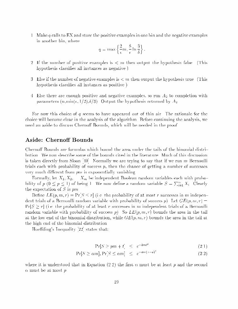
For now this choice of q seems to have appeared out of thin air. The rationale for thechoice will become clear in the analysis of the algorithm. Before continuing the analysis, weneed an aside to discuss Cherno� Bounds, which will be needed in the proof.
Aside: Cherno� Bounds
Cherno� Bounds are formulas which bound the area under the tails of the binomial distri-bution. We now describe some of the bounds cited in the literature. Much of this discussion
is taken directly from Sloan [40]. Normally we are trying to say that if we run m Bernoullitrials each with probability of success p, then the chance of getting a number of successesvery much di�erent from pm is exponentially vanishing.
Formally, let X1;X2; . . .Xm be independent Boolean random variables each with proba-bility of p (0 � p � 1) of being 1. We now de�ne a random variable S =
Pmi=1Xi. Clearly
the expectation of S is pm.
De�ne LE(p;m; r) = Pr[S � r] (i.e. the probability of at most r successes in m indepen-
dent trials of a Bernoulli random variable with probability of success p). Let GE(p;m; r) =Pr[S � r] (i.e. the probability of at least r successes in m independent trials of a Bernoullirandom variable with probability of success p). So LE(p;m; r) bounds the area in the tail
at the low end of the binomial distribution, while GE(p;m; r) bounds the area in the tail at
the high end of the binomial distribution.
Hoe�ding's Inequality [22] states that:
Pr[S � pm + t] � e�2mt2
(2.1)
Pr[S � �m];Pr[S � �m] � e�2m(��p)2 (2.2)
where it is understood that in Equation (2.2) the �rst � must be at least p and the second
� must be at most p.
19
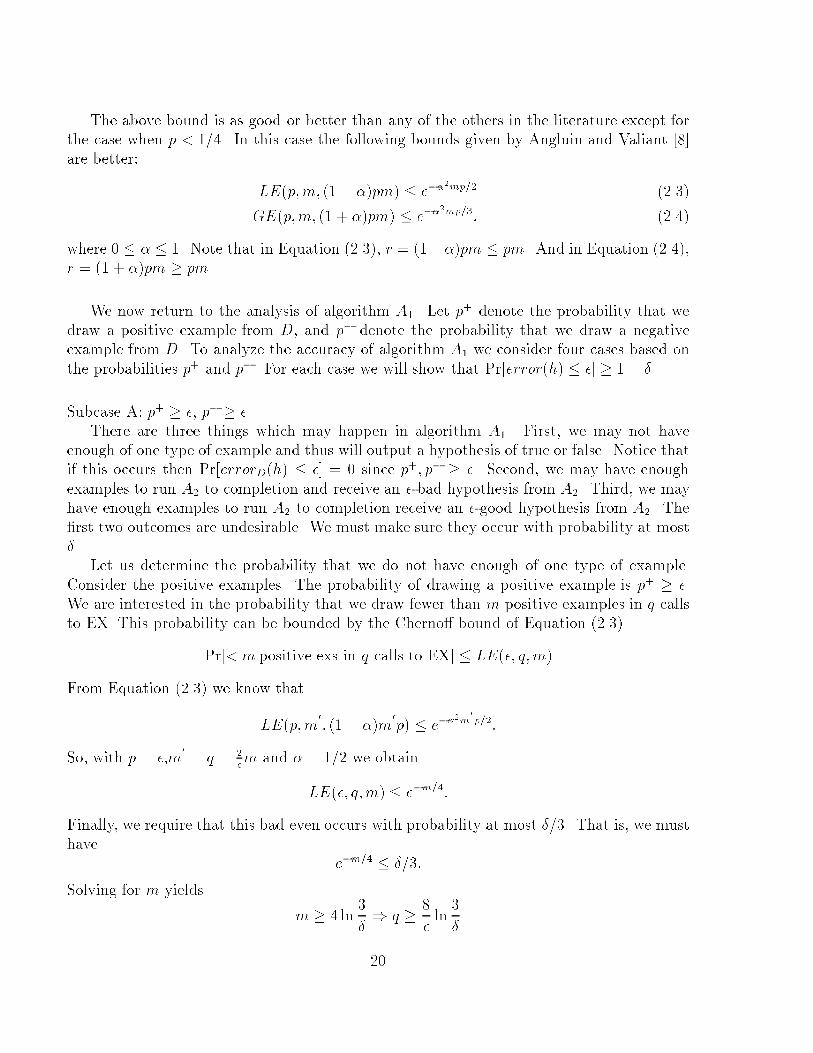
The above bound is as good or better than any of the others in the literature except for
the case when p < 1=4. In this case the following bounds given by Angluin and Valiant [8]
are better:
LE(p;m; (1� �)pm) � e��2mp=2 (2.3)
GE(p;m; (1 + �)pm) � e��2mp=3: (2.4)
where 0 � � � 1. Note that in Equation (2.3), r = (1��)pm � pm. And in Equation (2.4),
r = (1 + �)pm � pm.
We now return to the analysis of algorithm A1. Let p+ denote the probability that we
draw a positive example from D, and p� denote the probability that we draw a negative
example from D. To analyze the accuracy of algorithm A1 we consider four cases based on
the probabilities p+ and p�. For each case we will show that Pr[error(h) � �] � 1 � �.
Subcase A: p+ � �, p� � �.There are three things which may happen in algorithm A1. First, we may not have
enough of one type of example and thus will output a hypothesis of true or false. Notice thatif this occurs then Pr[errorD(h) � �] = 0 since p+; p� � �. Second, we may have enough
examples to run A2 to completion and receive an �-bad hypothesis from A2. Third, we mayhave enough examples to run A2 to completion receive an �-good hypothesis from A2. The�rst two outcomes are undesirable. We must make sure they occur with probability at most�.
Let us determine the probability that we do not have enough of one type of example.
Consider the positive examples. The probability of drawing a positive example is p+ � �.We are interested in the probability that we draw fewer than m positive examples in q callsto EX. This probability can be bounded by the Cherno� bound of Equation (2.3).
Pr[< m positive exs in q calls to EX] � LE(�; q;m)
From Equation (2.3) we know that
LE(p;m0
; (1� �)m0
p) � e��2m
0
p=2:
So, with p = �,m0
= q = 2�m and � = 1=2 we obtain
LE(�; q;m) � e�m=4:
Finally, we require that this bad even occurs with probability at most �=3. That is, we musthave
e�m=4 � �=3:
Solving for m yields
m � 4 ln3
�) q �
8
�ln
3
�
20
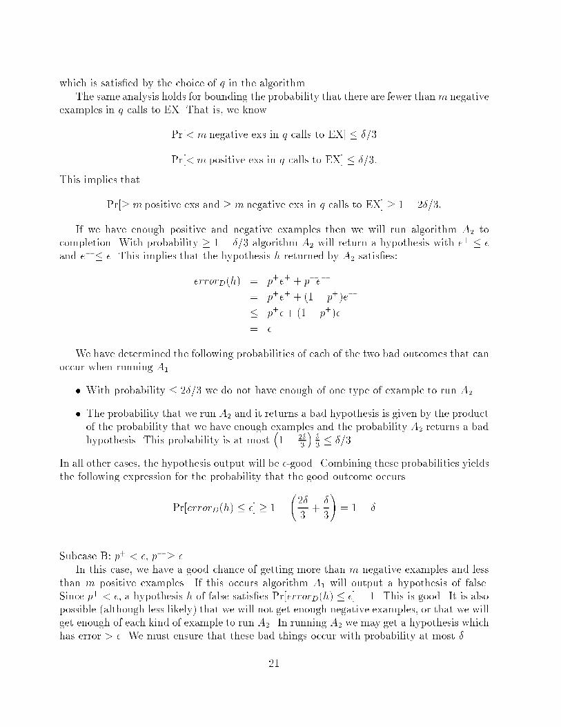
which is satis�ed by the choice of q in the algorithm.
The same analysis holds for bounding the probability that there are fewer than m negative
examples in q calls to EX. That is, we know
Pr[< m negative exs in q calls to EX] � �=3
Pr[< m positive exs in q calls to EX] � �=3:
This implies that
Pr[� m positive exs and � m negative exs in q calls to EX] � 1 � 2�=3:
If we have enough positive and negative examples then we will run algorithm A2 to
completion. With probability � 1 � �=3 algorithm A2 will return a hypothesis with e+ � �
and e� � �. This implies that the hypothesis h returned by A2 satis�es:
errorD(h) = p+e+ + p�e�
= p+e+ + (1� p+)e�
� p+�+ (1 � p+)�
= �
We have determined the following probabilities of each of the two bad outcomes that canoccur when running A1.
� With probability � 2�=3 we do not have enough of one type of example to run A2.
� The probability that we run A2 and it returns a bad hypothesis is given by the productof the probability that we have enough examples and the probability A2 returns a bad
hypothesis. This probability is at most�1� 2�
3
��3� �=3.
In all other cases, the hypothesis output will be �-good. Combining these probabilities yieldsthe following expression for the probability that the good outcome occurs.
Pr[errorD(h) � �] � 1 �
2�
3+�
3
!= 1 � �
Subcase B: p+ < �, p� � �.
In this case, we have a good chance of getting more than m negative examples and less
than m positive examples. If this occurs algorithm A1 will output a hypothesis of false.Since p+ < �, a hypothesis h of false satis�es Pr[errorD(h) � �] = 1. This is good. It is also
possible (although less likely) that we will not get enough negative examples, or that we will
get enough of each kind of example to run A2. In running A2 we may get a hypothesis whichhas error > �. We must ensure that these bad things occur with probability at most �.
21
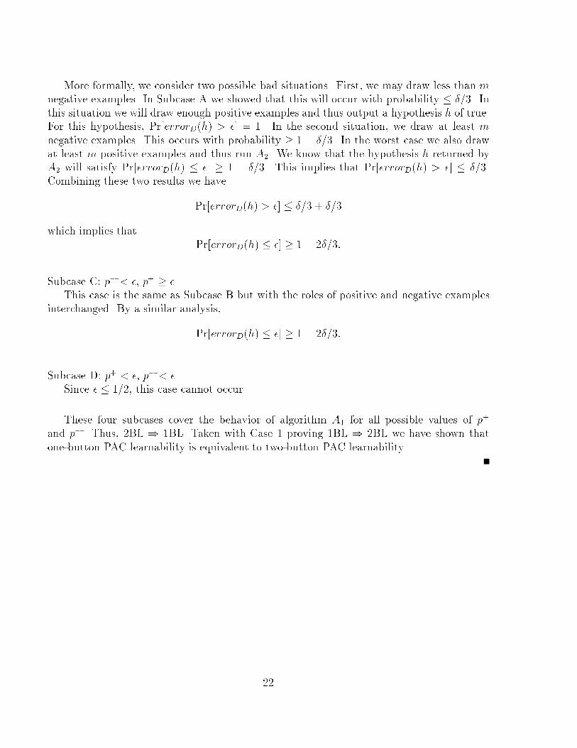
More formally, we consider two possible bad situations. First, we may draw less than m
negative examples. In Subcase A we showed that this will occur with probability � �=3. In
this situation we will draw enough positive examples and thus output a hypothesis h of true.
For this hypothesis, Pr[errorD(h) > �] = 1. In the second situation, we draw at least m
negative examples. This occurs with probability � 1 � �=3. In the worst case we also draw
at least m positive examples and thus run A2. We know that the hypothesis h returned by
A2 will satisfy Pr[errorD(h) � �] � 1 � �=3. This implies that Pr[errorD(h) > �] � �=3.
Combining these two results we have
Pr[errorD(h) > �] � �=3 + �=3
which implies that
Pr[errorD(h) � �] � 1� 2�=3:
Subcase C: p� < �, p+ � �.This case is the same as Subcase B but with the roles of positive and negative examples
interchanged. By a similar analysis,
Pr[errorD(h) � �] � 1� 2�=3:
Subcase D: p+ < �, p� < �.Since � � 1=2, this case cannot occur.
These four subcases cover the behavior of algorithm A1 for all possible values of p+
and p�. Thus, 2BL ) 1BL. Taken with Case 1 proving 1BL ) 2BL we have shown that
one-button PAC learnability is equivalent to two-button PAC learnability.
22
CS 582T Computational Learning Theory Spring Semester, 1991
Topic 3: Learning k-term-DNF
Lecturer: Sally Goldman Scribe: Weilan Wu
3.1 Introduction
In this lecture, we shall discuss the learnability of k-term-DNF formulas. Most of the material
presented in this lecture comes from the paper \Computational Limitations on Learning from
Examples," by Leonard Pitt and Leslie Valiant [33].
When introducing the PAC model, we showed that both k-CNF and k-DNF are PAClearnable using a hypothesis space of k-DNF and k-CNF respectively. Does a similar resulthold for k-term-DNF and k-clause-CNF? We �rst show that k-term-DNF is not PAC learn-able by k-term-DNF in polynomial time, unless RP=NP. In fact, this hardness result holds
even for learning monotone k-term-DNF by k-term-DNF. Likewise, k-clause-CNF is not PAClearnable by k-clause-CNF in both the monotone and unrestricted case. Contrasting thesenegative results, we then describe an e�cient algorithm to learn k-term-DNF by k-CNF. Asa dual result, we can learn k-clause-CNF using the hypothesis space of k-DNF. Finally, weexplore the representational power of the concept classes that we have considered so far and
the class of k-decision-lists [35].
Before describing the representation-dependent hardness result, we �rst give some basicde�nitions. The concept class of k-term-DNF is de�ned as follows:
De�nition 3.1 For any constant k, the class of k-term-DNF formulas contains all disjunc-tions of the form T1 _ T2 _ . . . _ Tk, where each Ti is monomial.
Up to now we have assumed that in the PAC model the hypothesis space available to
the learner is equivalent to the concept class. That is, each element of the hypothesis spacecorresponds to the representation of an element of the concept space. However, in generalone can talk about a concept class C being PAC learnable by H (possibly di�erent from C).
Formally, we say that C is PAC learnable by H, if there exists a polynomial-time learning
algorithm A such that for any c 2 C, any distribution D and any �, �, A can output withprobability at least 1 � � a hypothesis h 2 H such that h has probability at most � of
disagreeing with c on a randomly drawn instance from D.
3.2 Representation-dependent Hardness Results
In this section, we will show that for k � 2, k-term-DNF is not PAC learnable using a
hypothesis from k-term-DNF. This type of hardness result is representation-dependent since
23
it only holds if the learner's hypothesis class (or representation class) is restricted to be a
certain class. Note that when k = 1, the class of k-term-DNF formulas is just the class of
monomials, which we know is learnable using a hypothesis of a monomial.
We prove this hardness result by by reducing the learning problem to k-NM-Colorability,
a generalization of the Graph k-Colorability problem. Before de�ning this problem we �rst
describe two known NP-complete problems: Graph k-colorability (NP-complete for k � 3)
and Set Splitting. These descriptions come from Garey and Johnson [14].
Problem: Graph k-colorability
Instance: For a graph G = (V;E), with positive integer k � jV j.Question: Is G k-colorable? That is, does there exist a function f : V ! f1; . . . ; kg, such
that f(u) 6= f(v) whenever fu; vg 2 E?
Problem: Set SplittingInstance: Collection C of subsets of a �nite set S.Question: Is there a partition of S into two subsets S1; S2, such that no subset in C isentirely contained in either S1 or S2?
We now generalize both of these problems to obtain the k-NM-Colorability problem whichwe use for our reduction.
Problem: k-NM-Colorability
Instance: A �nite set S and a collection C = fc1; . . . ; cmg of constraints ci � S.Question: Is there a k-coloring � of the elements of S, such that for each constraints ci 2 C,the elements of ci are not MONOCHROMATICALLY colored (i.e. 8ci 2 C; 9x; y 2 ci, suchthat �(x) 6= �(y))?
We now argue that k-NM-Colorability is NP-complete. Clearly k-NM-Colorability is inNP. Note that if every ci 2 C has size 2, then the k-NM-Colorability problem is simply the
Graph-k-Colorability problem. Since the Graph-k-Colorability is NP-complete for k � 3, weonly need to show that 2-NM-Colorability is NP-hard. However, note that 2-NM-Colorabilityis exactly the Set Splitting problem which is NP-complete. Thus it follows that k-NM-
Colorability is NP-complete.
We now prove the main results of this section that k-term-DNF is not PAC learnable byk-term-DNF.
Theorem 3.1 For all integers k � 2, k-term DNF is not PAC learnable (in polynomialtime) using a hypothesis from k-term-DNF unless RP=NP.
Proof: We reduce k-NM-coloring to the k-term-DNF learning problem. Let (S;C) be an
instance of k-NM-coloring, we construct a k-term-DNF learning problem as follows: Each
instance (S;C) will correspond to a particular k-term-DNF formula to be learned. If S =fs1; . . . ; sng, then we will create n variables fx1; . . . ; xng for the learning problem. We now
describe the positive and negative examples, as well as the distributions D+ and D�.
� The positive examples are f~pigni=1, where ~pi is the vector with xi=0, and for j 6= i,
24
xj=1. Thus there are n positive examples. Finally, let D+ be uniform over these
positive examples (i.e. each has weight 1=n).
� The negative examples are f~nigjCji=1, where for each constraint ci 2 C, if ci = fsi1; . . . ; simg,
then ~ni = ~0i1;i2;...;im (all elements of S in ci are 0, the others are 1). For exam-
ple, if the constraint ci is fs1; s3; s8g, then the vector corresponding to is: ~ni =<
0101111011 . . . >. Finally, let D� be uniform over these negative examples (so each
has weight 1=jCj).
We now show that a k-term-DNF formula is consistent with all the positive and negative
examples de�ned above if and only if (S;C) is k-NM-colorable. Then we use this claim to
show that the learning problem is solvable in polynomial time if and only if RP= NP.
Claim 3.1 There is a k-term-DNF formula consistent with all positive and negative exam-ples de�ned above if and only if (S;C) is k-NM-colorable.
Proof of Claim:
((=) Without loss of generality, assume that (S;C) is k-NM-colorable by a coloring � :
S ! f1; 2; . . . ; kg; which uses every color at least once. Let f be the k-term-DNF formulaT1 _ T2 _ . . . _ Tk, where
Ti =^
�(sj)6=i
xj:
In other words, Ti is the conjunction of all xj corresponding to sj that are not colored withi.
We now show that f is consistent with positive examples. The positive example ~pj(xj = 0, xi = 1 for all i 6= j) clearly satis�es the term Ti, where �(sj) = i. Thus, f is truefor all positive examples.
Finally, we show that f is consistent with the negative examples. Suppose some negative
example, say ~ni = ~0i1;...;im satis�es f , then ~ni satis�es some term, say Tj. Then every elementof constraint ci = fsi1 ; . . . ; simg must be colored j, (They are 0 in ~ni and thus must not be
in Tj, hence they are colored with j). But then ci is monochromatic, giving a contradiction.
(=)) Suppose T1 _ . . . _ Tk is a k-term-DNF formula consistent with all positive examplesand no negative examples. We now show that, without loss of generality, we can assume for
all i, Ti is a conjunction of positive literals.
Case 1: Ti contains at least two negated variables. However, all positive examples have asingle 0, so none could satisfy Ti. Thus just remove Ti.
Case 2: Ti contains 1 negated variable xj. Then Ti can only be satis�ed by the singlepositive example ~pj . In this case, replace Ti by T 0
i =Vj 6=i xj, which is satis�ed only by
the vectors ~pj and ~1, neither of which are negative examples.
25
Thus we now assume that all terms are a conjunction of positive literals. Now color
the elements of S by the function: � : S ! f1; . . . ; kg, de�ned by �(si) = minfj :
xi does not occur in Tjg.Now we show � is well de�ned. Since each positive example pi satis�es T1 _ . . . _ Tk, it
must satisfy some term Tj. But each term is a conjunct of unnegated literals. Thus for some
j, xi must not occur in Tj. Thus each element of S receives a color (which is clearly unique).
Finally we show that � obeys the constraints. Suppose � violates constraint ci, then all
of the elements in ci are colored by the same color, say j. By the de�nition of �, none of
the literals corresponding to elements in ci occur in term Tj, so the negative example ~niassociated with ci satis�es Tj. This contradicts the assumption that none of the negative
examples satisfy the formula T1 _ . . . _ Tk. This completes the proof of the claim.
We now complete the proof of the theorem. Namely, we show how a learning algorithm
for k-term-DNF can be used to decide k-NM -colorability in random polynomial time. Firstwe give the de�nition of complexity class RP.
De�nition 3.2 A set S is accepted in the random polynomial time (i.e. S is in RP ) if there
exists a randomized algorithm A such that on all inputs, A is guaranteed to halt in polynomialtime and, if x 62 S;A(x) =\no", if x 2 S;Pr[A(x) = \yes00] � 1=2.
Now we show that if there is a PAC learning algorithm for k-term-DNF, it can be usedto decide k-NM-colorability in randomized polynomial time. Given instance (S;C), let D+
and D� be de�ned as above. Choose � < 12, � < minf 1
jSj; 1jCjg.
If (S;C) is k-NM-Colorable, then by the above claim there exists a k-term-DNF formulaconsistent with the positive and negative examples, so with probability at least 1 � �, ourlearning algorithm will be able to �nd it.
Conversely, if (S;C) is not k-NM-Colorable, by the Claim, there does not exist a consis-tent k-term-DNF formula, and the learning algorithm must either fail to produce a hypothesisin the allotted time, or produce one that is not consistent with at least one example. In eithercase, this can be observed, and we can determine that no legal k-NM-coloring is possible.
Thus we have shown that for k � 2, k-term-DNF is not PAC learnable by k-term-DNF.
Furthermore, note that the target function f created in this proof is monotone and thus this
result holds even if the concept class is monotone k-term-DNF and the hypothesis class isk-term-DNF. Finally, a dual hardness result applies for learning k-clause-CNF by k-clause-
CNF.
3.3 Learning Algorithm for k-term-DNF
Although k-term-DNF is not PAC learnable by k-term-DNF, we now show that it is learnableusing a hypothesis from k-CNF.
Let f = T1 _ T2 _ . . . _ Tk be the target formula, where
T1 = y(1)1 ^ y
(1)2 ^ . . . ^ y(1)m1
26
T2 = y(2)1 ^ y
(2)2 ^ . . . ^ y(2)m2
......
Tk = y(k)1 ^ y
(k)2 ^ . . . ^ y(k)mk
and y(j)i represents one of the n variables.
By distributing, we can rewrite f as:
f =^
i1;i2;...;ik
(y(1)i1_ y
(2)i2_ . . . _ y
(k)ik
):
Now to learn f using a hypothesis form k-CNF, we introduce O(2nk) variables �1; �2; . . . ; �m,
representing all disjunctions of the form: y(1)i1_ y
(2)i2_ . . . _ y
(k)ik
. Learning the conjunction
over the �'s is equivalent to learning the original disjunction. Note, however, we may not(in general) transform the conjunction we obtain to a k-term-DNF formula, thus we mustoutput it as a k-CNF formula.
3.4 Relations Between Concept Classes
In this section, we brie y study the containment relations between various concept classes.We have already seen that k-term-DNF is a subclass of k-CNF. We now show that k-
term-DNF is properly contained in k-CNF by exhibiting a k-CNF formula which can not beexpressed as a k-term-DNF formula. The k-CNF formula, (x1_x2)^(x3_x4)^. . . (x2k�1_x2k),has 2k terms when we unfold it into the form of DNF formula and thus cannot be representedby a k-term-DNF formula.
As a dual result, it is easily shown that k-clause-CNF is properly contained in k-DNF.
Thus it follows that, k-CNF [ k-DNF [ k-term-DNF [ k-clause-CNF is PAC learnable.We now consider the concept class k-DL as de�ned by Rivest [35]. Consider a Boolean
function f that is de�ned on f0; 1gn by a nested if{then{else statement of the form:
f(x1; x2; . . . ; xn) = if l1 then c1 elseif l2 then c2 � � � elseif lk then ck else ck+1
where the lj's are literals (either one of the variables or their negations), and the cj's are
either T (true) or F (false). Such a function is said to be computed by a simple decision
list . The concept class k-decision lists (k-DL) is just the extension of a simple decision listwhere the condition in each if statement may be the conjunction of up to k literals, for some
�xed constant k. We leave it as a simple exercise to show that k-CNF [ k-DNF is properlycontained in k-DL. Thus the �rst problem of Homework 1 provides an even stronger positive
result by showing that k-DL is PAC learnable using a hypothesis from k-DL.
27

28
CS 582T Computational Learning Theory Spring Semester, 1991
Topic 4: Handling an Unknown Size Parameter
Lecturer: Sally Goldman
4.1 Introduction
We have seen in earlier notes how to PAC learn a k-CNF formula. Recall that the algorithm
used for learning k-CNF created a new variable corresponding to each possible term of at
most k literals and then just applied the algorithm for learning monomials. Observe thatthis algorithm assumes that the learner knows k a priori. Can we modify this algorithm towork when the learner does not have prior knowledge of k? Here we consider a variant ofthe PAC model introduced in Topic 1 in which there is an unknown size parameter. The
material presented in this lecture is just one portion of the paper, \Equivalence of Models forPolynomial Learnability," by David Haussler, Michael Kearns, Nick Littlestone, and ManfredWarmuth [21].
4.2 The Learning Algorithm
In this section we outline a general procedure to convert a PAC-learning algorithm A that
assumes a known size parameter s (e.g. the k in k-CNF) to a PAC-learning algorithm B thatworks without prior knowledge of s. As an example application, this procedure will enable usto convert our algorithms for learning k-CNF, k-CNF, k-term-DNF, k-clause-CNF, or k-DLinto corresponding algorithms that do not have prior knowledge of k. Observe, that whilethe learner does not know s, as one would expect the running time and sample complexity
of B will still depend on s. The most optimistic goal would be to have the time and samplecomplexity of B match that of A.
The basic idea of this conversion is as follows. Algorithm B will run algorithm A with an
estimate s for s such that this estimate is gradually increased. The key question is: How does
algorithm B know when its estimate for s is su�cient? The technique of hypothesis testingused to solve this problem is a general technique which is also useful in other situations.
Aside: Hypothesis Testing
We now describe a technique to test if a hypothesis is good. More speci�cally, given ahypothesis h, an error parameter �, and access to an example oracle EX we would like to
determine with high probability if h is an �-good hypothesis. Clearly it is not possible to
distinguish a hypothesis with error � from one with error just greater than �, however, we
29
can distinguish an �=2-good hypothesis from an �-bad one. As we shall see this is su�cient
to know when our estimate for the size parameter is large enough.
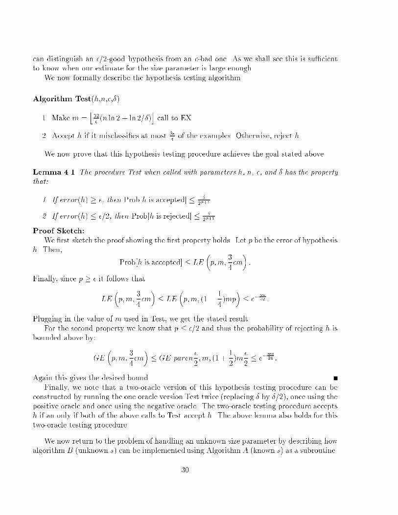
We now formally describe the hypothesis testing algorithm.
Algorithm Test(h,n,�,�)
1. Make m =j32�
(n ln 2 + ln 2=�)k
call to EX.
2. Accept h if it misclassi�es at most 3�4
of the examples. Otherwise, reject h.
We now prove that this hypothesis testing procedure achieves the goal stated above.
Lemma 4.1 The procedure Test when called with parameters h, n, �, and � has the propertythat:
1. If error(h) � �, then Prob[h is accepted] � �2n+1
2. If error(h) � �=2, then Prob[h is rejected] � �2n+1
Proof Sketch:
We �rst sketch the proof showing the �rst property holds. Let p be the error of hypothesish. Then,
Prob[h is accepted] � LE�p;m;
3
4�m
�:
Finally, since p � � it follows that
LE
�p;m;
3
4�m
�� LE
�p;m; (1�
1
4)mp
�� e�
m�32 :
Plugging in the value of m used in Test, we get the stated result.
For the second property we know that p � �=2 and thus the probability of rejecting h is
bounded above by:
GE
�p;m;
3
4�m
�� GE paren
�
2;m; (1 +
1
2)m
�
2� e�
m�24 :
Again this gives the desired bound.
Finally, we note that a two-oracle version of this hypothesis testing procedure can be
constructed by running the one oracle version Test twice (replacing � by �=2), once using the
positive oracle and once using the negative oracle. The two-oracle testing procedure acceptsh if an only if both of the above calls to Test accept h. The above lemma also holds for this
two-oracle testing procedure.
We now return to the problem of handling an unknown size parameter by describing how
algorithm B (unknown s) can be implemented using AlgorithmA (known s) as a subroutine.
30
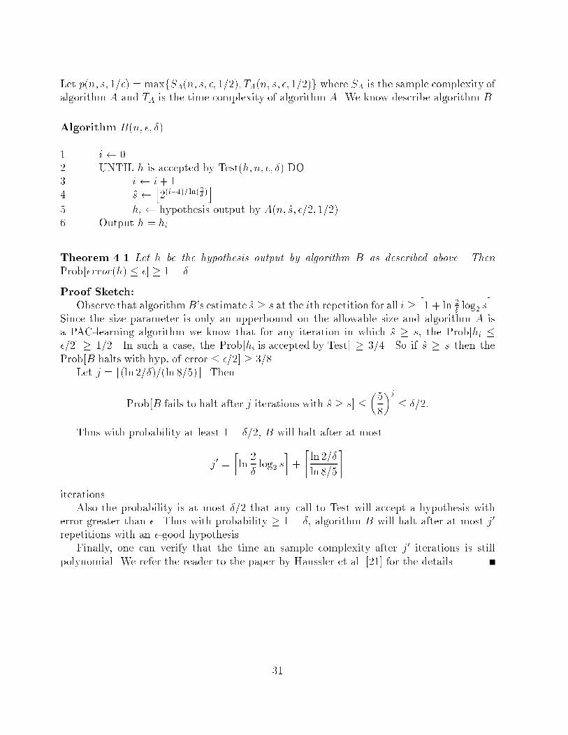
Let p(n; s; 1=�) = maxfSA(n; s; �; 1=2); TA(n; s; �; 1=2)g where SA is the sample complexity of
algorithm A and TA is the time complexity of algorithm A. We know describe algorithm B.
Algorithm B(n; �; �)
1 i 0
2 UNTIL h is accepted by Test(h; n; �; �) DO
3 i i+ 1
4 s j2(i�1)= ln(
2
�)k
5 hi hypothesis output by A(n; s; �=2; 1=2)
6 Output h = hi
Theorem 4.1 Let h be the hypothesis output by algorithm B as described above. ThenProb[error(h) � �] � 1 � �.
Proof Sketch:
Observe that algorithmB's estimate s � s at the ith repetition for all i �l1 + ln 2
�log2 s
m.
Since the size parameter is only an upperbound on the allowable size and algorithm A isa PAC-learning algorithm we know that for any iteration in which s � s, the Prob[hi ��=2] � 1=2. In such a case, the Prob[hi is accepted by Test] � 3=4. So if s � s then the
Prob[B halts with hyp: of error � �=2] � 3=8.Let j = b(ln 2=�)=(ln 8=5)c. Then
Prob[B fails to halt after j iterations with s � s] ��
5
8
�j� �=2:
Thus with probability at least 1� �=2, B will halt after at most
j0 =
�ln
2
�log2 s
�+
&ln 2=�
ln 8=5
'
iterations.
Also the probability is at most �=2 that any call to Test will accept a hypothesis with
error greater than �. Thus with probability � 1 � �, algorithm B will halt after at most j0
repetitions with an �-good hypothesis.Finally, one can verify that the time an sample complexity after j0 iterations is still
polynomial. We refer the reader to the paper by Haussler et al. [21] for the details.
31

32
CS 582T Computational Learning Theory Spring Semester, 1991
Topic 5: Learning with Noise
Lecturer: Sally Goldman Scribe: Gadi Pinkas
5.1 Introduction
Although up to now we have assumed that the data provided by the example oracle is noise-
free, in real-life learning problems this assumption is almost never valid. Thus we would like
to be able to modify our algorithms so that they are robust against noise. Before consideringlearning with noise in the PAC model, we must �rst formally model the noise. Although wewill only focus on one type of noise here, we �rst describe the various formal models of noisethat have been considered.
In all cases we assume that the usual noise free examples pass through a noise oraclebefore being seen by the learner. Each noise oracle represents some noise process beingapplied to the examples from EX. The output from the noise process is all the learner canobserve. The \desired," noiseless output of each oracle would thus be a correctly labeled
example (x; s), where x is drawn according to the unknown distribution D. We now describethe actual outputs from the following noise oracles:
Random Misclassi�cation Noise [7]: This noise oracle models a benign form of mis-classi�cation noise. When it is called, it calls EX to obtain some (noiseless) (x; s), andwith probability 1� �, it returns (x; s). However, with probability �, it returns (x; s).
Malicious Noise [44]: This oracle models the situation where the learner usually gets acorrect example, but some small fraction � of the time the learner gets noisy examplesand the nature of the noise is unknown or unpredictable. When this oracle is called,
with probability 1 � �, it does indeed return a correctly labeled (x; s) where x isdrawn according to D. With probability � it returns an example (x; s) about which no
assumptions whatsoever may be made. In particular, this example may be maliciouslyselected by an adversary who has in�nite computing power, and has knowledge of the
target concept, D, �, and the internal state of the learning algorithm.
Malicious Misclassi�cation Noise [41]: This noise oracle models a situation in whichthe only source of noise is misclassi�cation, but the nature of the misclassi�cation is
unknown or unpredictable. When it is called, it also calls EX to obtain some (noiseless)
(x; s), and with probability 1� �, it returns (x; s). With probability �, it returns (x; l)where l is a label about which no assumption whatsoever may be made. As with
malicious noise we assume an omnipotent, omniscient adversary; but in the case the
adversary only gets to choose the label of the example.
33
Uniform Random Attribute Noise [41]: This noise oracle models a situation where the
attributes of the examples are subject to noise, but that noise is as benign as possible.
For example, the attributes might be sent over a noisy channel. We consider this oracle
only when the instance space is f0; 1gn (i.e., we are learning Boolean functions). This
oracle calls EX and obtains some (x1 � � � xn; s). It then adds noise to this example by
independently ipping each bit xi to �xi with probability � for 1 � i � n. Note that
the label of the \true" example is never altered.
Nonuniform Random Attribute Noise [17]: This noise oracle provides a more realistic
model of random attribute noise than uniform random attribute noise.2 This oracle
also only applies when we are learning Boolean functions. This oracle calls EX and
obtains some (x1 � � � xn; s). The oracle then adds noise by independently ipping each
bit xi to �xi with some �xed probability �i � � for each 1 � i � n.
In this paper we focus on the situation in which there is random misclassi�cation noise.The material presented here comes from the paper \Learning from Noisy Examples," by DanaAngluin and Phil Laird [7]. We show that the hypothesis that minimizes disagreements (i.e.the hypothesis that misclassi�es the fewest training examples) meets the PAC correctness
criterion when the examples are corrupted by random misclassi�cation noise. Unfortunately,this technique is most often computationally intractable. However, for k-CNF formulas wedescribe an e�cient PAC learning algorithm that works against random misclassi�cationnoise. Both positive results need only assume that the noise rate � is less than one half.
Before describing these results, we brie y review what is known about handling the otherforms of noise. Sloan [41] has extended the above results to the case of malicious labelingnoise. On the other hand, Kearns and Li [25] have shown that the method of minimizingdisagreements can only tolerate a small amount of malicious noise. We will study this result
in Topic 15.
Unlike the results for labeling noise, in the case of uniform random attribute noise, ifone uses the minimal disagreement method, then the minimum error rate obtainable (i.e.
the minimum \epsilon") is bounded below by the noise rate [41]. Although the method ofminimizing disagreements is not e�ective against random attribute noise, there are techniques
for coping with uniform random attribute noise. In particular, Shackelford and Volper [38]
have an algorithm that tolerates large amounts of random attribute noise for learning k-DNF formulas. That algorithm, however, has one very unpleasant requirement: it must be
given the exact noise rate as an input. Goldman and Sloan [17] describe an algorithm forlearning monomials that tolerates large amounts of uniform random attribute noise (any
noise rate less than 1=2), and only requires some upper bound on the noise rate as an input.Finally, for nonuniform random attribute noise, Goldman and Sloan [17] have shown that
the minimum error rate obtainable is bounded below by one-half of the noise rate, regardless
of the technique (or computation time) of the learning algorithm.
2Technically, this oracle speci�es a family of oracles, each member of which is speci�ed by n variables,�1; . . . ; �n, where 0 � �i � �.
34
5.2 Learning Despite Classi�cation Noise
Let EX� be the random misclassi�cation noise oracle with a noise noise rate of �. Thus the
standard noise free oracle is EX0. Also we will use the notation that C = fL1; L2; . . . ; LNgwhere L� is the target concept. So we only consider the simple case of a �nite set of
hypothesis.
In this section we will study the random misclassi�cation model and give an algorithm
to PAC learn any �nite concept space with polynomial sample size (not necessarily with
polynomial time). In the next section we show that for � < 1=2, the class of k-CNF formulas
is PAC learnable from EX�. Observe that the learning problem is not feasible for � � 1=2.
If � = 1=2 the noise distorts all the information and clearly no learning is possible, and when
� > 1=2, we actually learn the complement concept with � < 1=2.
For now we assume that the learner has an upper bound �b on the noise rate. That is,� � �b < 1=2. Later we show how to remove this assumption. As one would expect if �b isvery close to 1=2, we must allow the learner more time and data. In fact, we will requirethat the time and sample complexity of the learner are polynomial in 1=(1 � 2�b). Observethat this quantity is inversely proportional to how close �b is to 1/2.
5.2.1 The Method of Minimizing Disagreements
Our goal in this section is to study the sample complexity for PAC learning under randommisclassi�cation noise. For the noise-free case we have seen that if Li agrees with at leastm � (1=�)(ln jCj+ ln(1=�)) = (1=�) ln(N=�) samples drawn from EX0 then Pr[error(Li) ��] � �. How much more data is needed when there is random misclassi�cation noise?
In the presence of noise the above approach will fail because there is no guarantee that
any hypothesis will be consistent with all the examples. However, if we replace the goal ofconsistency with that of minimizing the number of disagreements with the examples andpermit the sample size to depend on �b, we get an analogous result for the noisy case.
We shall use the following notation in formally describing the method of minimizingdisagreements.
� Let � be the sequence of examples drawn from EX�.
� Let F (Li; �) be the number of times Li disagrees with � on an example in �, where Lidisagrees with � on an example (~x; l) 2 � if and only if Li classi�es ~x di�erently froml.
Theorem 5.1 If we draw a sequence � of
m �2
�2(1 � 2�b)2ln
�2N
�
�
samples from EX� and �nd any hypothesis Li that minimizes F (Li; �) then
Pr[error(Li) � �] � �
35
.
Proof: We shall use the following notation in the proof. Let di be the error(Li). That
is, di is the probability that Li misclassi�es a randomly drawn example. Let pi be the
probability that an example from EX� disagrees with Li. Observe that pi is the probability
that Li misclassi�es a correctly labeled example (di(1 � �)), plus the probability that Licorrectly classi�es the example but the example has been improperly labeled by the noise
oracle ((1� di)�). Thus
pi = di(1� �) + (1� di)� = � + di(1 � 2�)
Note that for the right hypothesis (Li = L�), di = 0 and therefore pi = � (i.e., disagreements
are only caused by noise). Since � < 1=2, it follows that for any hypothesis pi � �. So all
hypothesis have an expected rate of disagreement of at least �.
Let an �-bad hypothesis be one for which di � �. Then for any �-bad hypothesis Li, wehave
pi � � + �(1� 2�):
Thus we have a separation of at least �(1 � 2�) between the disagreement rates of the
correct and an �-bad hypothesis. Although �b is not known, we know that � � �b < 1=2thus the minimum separation (or gap) is at least �(1 � 2�b). We take advantage of thisgap in the following manner. We will draw enough examples from EX� to guarantee withhigh probability that no �-bad hypothesis has a observed disagreement rate greater than� + �(1 � 2�b)=2. Similarly, we will draw enough examples from EX� to guarantee withhigh probability that the correct hypothesis has on observed disagreement rate less than
� + �(1 � 2�b)=2. Thus it follows that with high probability L� will have a lower observedrate of disagreement than any �-bad hypothesis. Thus by selecting the hypothesis with thelowest observed rate of disagreement, the learner knows (with high probability) that thishypothesis has error at most �.
We now formalize this intuition. We will draw m examples from EX� and compute anempirical estimate for all pi. That is, we compute F (Li; �) for every Li in the hypotheses
space. The hypothesis output will be the hypothesis Li that has the minimum estimate
for pi. What is the probability that Li is �-bad? Let s = �(1 � 2�b). In order for some
�-bad hypothesis Li to minimize F (Li; �) either the correct hypothesis must have a highdisagreement rate
F (L�; �)=m � � + s=2
or an �-bad hypothesis must have a low disagreement rate (� � + s=2). Finally, assumingthat neither of these bad events occur, since we select the hypothesis Li that minimizes thedisagreement rate we know that:
F (Li; �)=m < � + s=2
and thus Li has error of at most �.
36
Applying Cherno� bounds for the probability that a good hypothesis has high disagree-
ment:
Pr[F (L�; �)=m � � + s=2] = GE(�;m;m(� + s=2) < �=(2N) < �=2:
And if Li is �-bad then its probability to have low disagreement is:
Pr[F (L�; �)=m � � + s=2] = LE(� + s;m;m(� + s=2) � �=(2N):
Thus the probability that any �-bad hypothesis Li has F (Li; �)=m � �+ s=2 is at most �=2.
(There are at most N � 1 hypothesis that are �-bad.) Putting these two equalities together,
the probability that some �-bad hypothesis minimizes F (Li; �) is at most �.
Thus we know that by using the method of minimizing disagreements one can tolerate any
noise rate strictly less than 1=2. Furthermore, if the hypothesis minimizing disagreementscan be found in polynomial time then we obtain an e�cient PAC algorithm for learning
when there is random misclassi�cation noise.
5.2.2 Handling Unknown �b
Until now we have assumed the learner is given an upperbound �b on the noise rate. What if
such an upperbound is not known? We can solve this problem using the technique describedin Topic 4 for handling an unknown size parameter. That is, just treat � as the unknown sizeparameter. The only detail we need to worry about here is how to perform the hypothesistesting. The basic idea is as follows, we draw some examples and estimate the failureprobability of each of the hypotheses L1; :::; LN. The smallest estimate is compared to the
current value of �b. If the estimate pi is less than the current value of �b, we halt; otherwisewe increase �b and repeat. For details see the Angluin, Laird paper [7].
5.2.3 How Hard is Minimizing Disagreements?
How hard is to �nd an hypothesis Li that minimizes F (Li; �)? Unfortunately, the answer isthat is usually quite hard. For example consider the domain of all conjunctions of positive
literals (monotone monomials). To �nd a monotone monomial that minimizes the disagree-
ment is a NP-hard problem.
Theorem 5.2 Given a positive integer n and c and a sample �. The problem of determining
if is there a monotone monomial over n variables such that F (�; �) � c is NP-complete.
The result indicates that even for a very simple domain, the approach of directly trying
to minimize the disagreement is unlikely to be computationally feasible. However, in the
next section we show that for some concept classes, we can bypass the minimization problem(which is hard) and e�ciently PAC learn the concepts from noisy examples.
37
5.3 Learning k-CNF Under Random Misclassi�cation
Noise
In the previous section we described how to PAC learn any �nite concept space if we remove
the condition that our algorithm runs in polynomial time. However, we would like to have
e�cient algorithms for dealing with noise. In this section we use some of the ideas suggested
by the method of minimizing disagreements to get a polynomial time algorithm for PAC
learning k-CNF formulas using examples from EX�.
5.3.1 Basic Approach
Instead of searching for the k-CNF formula with the fewest disagreements, we will test all
potential clauses individually, and include those that are rarely false in a positive example.Of course, if a clause is false yet the example is reported as positive then either the clause
is not in the target formula, or the label has been inverted by the noise process. Thus if aclause is false on a signi�cant number of positive examples, then we do not want to includethe clause in our hypothesis. Observe that we will not be solving an NP-complete problem,the k-CNF formula that is chosen may not minimize the disagreements with the examples,but it will (with probability � 1 � �) have an error that is less then �.
We now give some notation that we use in this section.
� Let M be the number of possible clauses of at most k literals (M � (2n+ 1)k), and letC be any such clause.
� Let �� be the target k-CNF formula
� For all clauses C, let P00(C) = Prob[C is false and �� is false].
� For all clauses C, let P01(C) = Prob[C is false but �� is true].
� For all clauses C, let P0(C) = P00(C) + P01(C) = Prob[C is false].
Finally, we need the following two de�nitions. We say that a clause C is importantif and only if P0(C) � QI = �=(16M2). We say a clause C is harmful if and only ifP01(C) � QH = �=(2M). Note that QH � QI , so every harmful clause is important. Also,
no clause contained in �� can be harmful, since if �� classi�es an example as positive, the
example satis�es all its clauses and C must be true (i.e., P01(C) = 0).
The algorithm to PAC learn k-CNF formulas works as follows. We must construct an
hypothesis h that is �-good with high probability. To achieve this goal the hypothesis h
must have all the important clauses that are not harmful. A non-important clause is almostalways assigned the value \true" (by the examples in EX�), and thus it does not mater if
it is included in h or not. On the other hand, a harmful clause must not be included in h,
since it is very likely to be falsi�ed by a positive example.
38
Thus our goal is to �nd an hypothesis h that includes all important clauses and does
not include any harmful clause. We �rst prove that if we �nd such a hypothesis h then it is
�-good. Then we show how to e�ciently construct such a hypothesis with high probability.
Lemma 5.1 Let D be a �xed unknown distribution, and let �� be a �xed unknown target.
Let � be any conjunction (product) of clauses that contains every important clause in �� and
no harmful clauses. Then error(�) � �.
Proof: The probability that � misclassi�es an example from D is equal to the probability
that �� classi�es the example as positive but � classi�es it as negative, or vice versa (the
example is truly negative but � classi�es it as positive).
The probability of an error on a positive example is equal to the probability that any clause
in �� �� is falsi�ed by positive example; therefore,
Prob[�� = 1 ^ � = 0] �X
C2����
P01(C) < MQH = �=2
since there are at most M clauses in � and none are harmful.
The probability of error on a negative example is equal to the probability that a clausein �� � � is falsi�ed and all clauses in � are true. This probability is less or equal to theprobability that a clause in �� � � is falsi�ed. Since � contains all the important but notharmful clauses and �� contains no harmful clauses, then ���� contains only non-importantclauses. Therefore,
Prob[� = 1 ^ �� = 0] �X
C2����
P0(C) < MQI = �=(16M) < �=2
Thus,
error(�) � Prob[� = 1 ^ �� = 0] + Prob[� = 0 ^ �� = 1] � �=2 + �=2 = �:
To complete the algorithm for learning k-CNF under noise, we must construct an e�cientalgorithm to �nd a formula � that contains all the important clauses and no harmful clauses(with high probability). Observe that we have no direct information about whether a clause
is important or harmful. More speci�cally, we cannot directly compute P00(C) or P01(C),
but rather must rely on the examples received from EX�. However, since EX� only modi�esthe label and not the values of the attributes in the example, P0(C) can be directly estimated
by drawing a sample from EX�, and calculating the fraction of the assignments that assign\false" to C. Thus we can accurately estimate P0(C) for every possible clause and thus
decide (with high probability) which clauses are important. Let I be the set of clauses that
are determined to be important. The only thing left, is to identify the harmful clauses in I
and eliminate them.
Harmful clauses are those that are falsi�ed by positive examples (examples that satisfy��), but since the classi�cation of the example is subject to noise we cannot directly estimate
39
P01(C). Let P0+(C) be the probability that a a clause is falsi�ed by an example and that
EX� reports that the example is positive. This probability can be directly estimated by
counting the number of examples from the sample that are reported as positive and falsify
the clause C. We perform this estimate for every important clause. For the estimate of
P0+(C), an example is counted if and only if the example is positive and no error occurred
in the reporting, or the example is negative and there was an error in the reporting. Thus,
P0+(C) = (1 � �)P01(C) + �P00(C)
= �(P00(C) + P01(C)) + (1� 2�)P01(C)
= �P0(C) + (1� 2�)P01(C)
If P0(C) 6= 0, then the proportion of examples falsifying C that are reported as positive is:
P0+(C)
P0(C)= � +
P01(C)
P0(C)(1 � 2�)
and since � < 1=2, we get:P0+(C)
P0(C)� �:
We would like to separate between two cases: one is the case where C is a desired clause(C 2 ��) and the other is when C is harmful. If C 2 �� then
P0+(C)
P0(C)= �;
while if C is harmful (P01(C) � QH):
P0+(C)
P0(C)� � +QH(1� 2�) � � +
�
2M(1� 2�):
Thus, we have a separation of at least s = QH(1� 2�) between the clauses that are included
in �� and the harmful clauses. Since � � �b, the separation is bounded bellow by s =QH(1 � 2�b).
If we knew the value of �, we could estimate P0+=P0 for all clauses and delete from I all
the clauses with an estimate that is greater than � + s=2. However, we do not know � andthus we do not know where the cuto� is.
How can we estimate �? If I contains any clause C that is also in �� then the estimateof P0+(C)=P0(C) will be close to �. So we can take the minimum of this value over all the
clauses in I as a �rst estimate for �:
� = minc2I
P0+(C)
P0(C):
If no clause in I is contained also in ��, then the estimate � calculated above may not bea good estimate of �. However, since I contains all the important clauses it must be that
40
�� contains no important clauses. This means that most of the examples drawn from D
satisfy these non-important clauses and therefore satisfy ��. In this case most examples are
positive, and thus the observed overall rate of negative examples is su�ciently close to �.
Thus, the estimate of � is taken to be the minimum of the two estimates:
� = min
(fraction of negative examples;min
c2I
(P0+(C)
P0(C)
)):
We use therefore � + s=2 to decide which are the harmful clauses.
5.3.2 Details of the Algorithm
We now put these ideas together to get an e�cient algorithm for PAC learning k-CNF
formulas under random misclassi�cation noise.
Algorithm Learn-Noisy-k-CNF(n,k,�,�,�b)
1. m = d 210M4
�3(1��b)2ln(6M
�)e, where M is the number of possible clauses
2. QI = �=(16M2);QH = �=2M ; sb = QH(1 � 2�b)
3. We draw m examples from the oracle EX�, and set: P� = number of negative examples
in the sample
4. For each possible clause C, we compute:
(a) P0(C) = the number of examples that falsify the clause C
(b) P0+(C) = the number of positive (reported) examples that falsify C
(c) If P0(C) 6= 0 then h(C) = P0+(C)=P0(C).
(d) �1 = P�=m, the observed fraction of negative examples
5. Form the set I by including all the important clauses C; i.e., P0(C)=m � QI=2
6. �2 = minc2Ifh(C)g
7. � = minf�1; �2g
8. The �nal output � is the conjunction (product) of all those clauses C 2 I such that
h(C) � � + sb=2
To prove that the algorithm is correct, we need to prove that � contains all important
clauses that are not harmful (with probability greater than 1 � �). Only in the following
cases the algorithm could go wrong:
� Some important clauses might not be selected for inclusion in I.
41
� the estimate � could be too large (� � � + s=4) or too small (� � � � s=4).
� Some harmful clauses may be included in �.
� Some correct clauses may be excluded from �.
The proof uses Cherno� bounds, showing that the second case has a probability of at
most �=2, while the other cases, each has a probability of at most �=6. Therefore, the toatl
probability of error is at most �, and by the previous lemma, the output formula is �-good
with high probability. For the details of the proof, see the Angluin, Laird paper[7].
42
CS 582T Computational Learning Theory Spring Semester, 1991
Topic 6: Occam's Razor
Lecturer: Sally Goldman Scribe: Nilesh Jain
\Entities should not be multiplied unnecessarily"
William of Occam, c. 1320
6.1 Introduction
The above quote is better known to us today as Occam's Razor or the Principle of OntologicalParsimony. Over the centuries, people from di�erent �elds have given it di�erent interpre-tations. One interpretation used by the experimental scientists is: given two explanations ofthe data, all other things being equal, the simpler explanation is preferable.
This principle is consistent with the goal of machine learning: to discover the simplesthypothesis that is consistent with the sample data. However, the question still remains: whyshould one assume that the simplest hypothesis based on past examples will perform well on
future examples. After all, the real value of a hypothesis is in predicting the examples thatit has not yet seen.
It will be shown that, under very general assumptions, Occam's Razor produces hypothe-
ses that with high probability will be predictive of future observations. As a consequence,when hypotheses of minimum or near minimum complexity can be produced in time poly-nomial in the size of the sample data, it leads to a polynomial PAC-learning algorithm.The material presented in the lecture comes from the paper \Occam's Razor," by AnselmBlumer, Andrzej Ehrenfeucht, David Haussler, and Manfred Warmuth [11]. Portion of the
notes are taken from this paper.
6.2 Using the Razor
In this section, we de�ne an Occam-algorithm and show that the existence of an Occam-
algorithm implies polynomial learnability. First, we prove the uniform convergence lemma.
Lemma 6.1 (Uniform Convergence Lemma) Given any function f in a hypothesis class
of r hypotheses, the probability that any hypothesis with error larger than � is consistent witha sample of size m is less than (1� �)m r.
Proof: Let hi be any hypothesis with error larger than �. The probability that hi isconsistent with one observation of f is less than (1� �). Since all the m samples of f are
drawn independent of each other, the probability that hi is consistent with all m observationsof f is less than (1 � �)m. Finally, since there are r hypothesis, the probability that any
43
hypothesis with error larger than � is consistent with all m observations of f is less than
(1� �)m r.For an in�nite hypothesis class, the learning algorithm would have to choose a hypothesis
carefully. Occam's Razor suggests that the learning algorithm should choose its hypothesis
among those that are consistent with the sample and have the minimum complexity. But
this may sometimes be intractable. For example, �nding a minimum length DNF expression
consistent with a sample of a Boolean function and �nding a minimum size DFA consistent
with a set of positive and negative examples of a regular language are known to be NP-
hard [14]. To obtain polynomial algorithms, the criterion is weakened as follows.
De�nition 6.1 An Occam-algorithm forH with constant parameters c � 1 and compression
factor 0 � � < 1 is a learning algorithm that given a sample of size m which is labeled
according to some hypothesis h 2 H:
1. produces a hypothesis consistent with the data, that is, all the observations can beexplained by the hypothesis,
2. produces a hypothesis of complexity at most ncm� where n is the complexity of h, and
3. runs in time polynomial in n and m.
We now show that the existence of an Occam-algorithm for H implies polynomial learn-ability.
Theorem 6.1 Given independent observations of any function in H of complexity at most
n, an Occam-algorithm with parameters c � 1 and 0 � � < 1 produces a hypothesis of errorat most � with probability at least 1 � � using sample size polynomial in n; 1=�, and 1=�,independent of the function and of the probability distribution. The sample size required is
O
1
�lg
�1
�
�+
�nc
�
�1=(1��)!:
Proof: Let the size of the hypothesis space be r. We will show that the Occam-algorithm
produces a good hypothesis after drawing a sample of size
m � max
8<: 2 lg (1=�)
� lg (1 � �);
2nc
� lg (1� �)
!1=(1��)9=;
Since the hypothesis under consideration are given by binary strings of length at most ncm�,
the size of the hypothesis space, r, is at most 2ncm�
.We �rst consider the second lower bound on m,
m �
2nc
� lg (1� �)
!1=(1��)
:
44
Raising both sides to the power of (1� �) yields
m1�� �2nc
� lg (1 � �):
Simplifying further we obtain
ncm� � �1
2m lg (1 � �) :
Finally, raising both sides to the power of 2 gives
2ncm�
� (1 � �)�m=2 :
Recall that r � 2ncm�
and thus it follows from above that:
r � (1 � �)�m=2 :
From the uniform convergence lemma, we get that:
Pr[any ��bad hyp: is consistent with m exs:] � (1� �)mr
� (1� �)�m=2(1� �)m
= (1� �)m=2: (6.1)
Finally, we consider the �rst lower bound on m,
m �2 lg (1=�)
� lg (1 � �):
Multiplying both sides by lg (1 � �) which is negative, we get
m
2lg (1� �) � � lg (1=�) = lg �:
Raising both sides to the power of 2 gives
(1 � �)m=2 � � (6:2)
We complete the proof by combining Equations (6.1) and (6.2) gives that the probability
that an �-bad hypothesis is consistent with all the m examples is at most �. Thus the
Occam-algorithm produces a good hypothesis after drawing m examples where
m = O
1
�lg�
1
�
�+
�nc
�
�1=(1��)!
By de�nition of an Occam-algorithm, it runs in time polynomial in n and m. Thus, we have
a PAC-learning algorithm.
45

46
CS 582T Computational Learning Theory Spring Semester, 1991
Topic 7: The Vapnik-Chervonenkis Dimension
Lecturer: Sally Goldman Scribe: Nilesh Jain
7.1 Introduction
In the notes on Occam's Razor, we de�ned the condition for uniform convergence on �nite
concept classes. We can state the general condition for uniform convergence as follows:
PrS2Dm
[9h 2 C jerrorD (h) > � ^ h is consistent with S] � �
where S is a set of m examples from the instance space X having probability distribution D.To determine whether a concept class C is uniformly learnable, we have to �nd out if thereexists a learning function A satisfying the above condition. If so, we say that C is uniformly
learnable and has sample complexity m.
For �nite concept classes, such uniform convergence proofs are easy because we know jCj.However, when the concept class is in�nite, we need some other measure to replace jCj. Sucha measure is a combinatorial parameter known as the Vapnik-Chervonenkis (VC) dimension.
The VC dimension of a concept class C is a measure of the complexity of the class.
In the next section, we will de�ne the VC dimension and some other concepts needed tode�ne the VC dimension. We shall then measure the VC dimension of some concept classes.The following section will contain the theorems relating the VC dimension to uniform learn-
ability and the sample complexity. Finally, we will see some relations on the VC dimension.The material presented in the lecture comes from the paper \Learnability and the Vapnik-Chervonenkis Dimension," by Anselm Blumer, Andrzej Ehrenfeucht, David Haussler, andManfred Warmuth [12]. Portions of the notes are taken from this paper.
7.2 VC Dimension De�ned
The de�nition of VC dimension uses the de�nition of a shattered set. We now give twoequivalent de�nitions for a shattered set. Let X be the instance space and C the concept
class.
De�nition 7.1 A �nite set S � X is shattered by C if for each subset S0 � S, there is a
concept c 2 C which contains all of S0 and none of S � S0.
In order to give the alternate de�nition of shattering, we �rst need the following de�nition.
47
De�nition 7.2 Given S � X, �C(S) denotes the set of all subsets of S that can be obtained
by intersecting S with a concept in C. Thus,
�C(S) = fS \ c : c 2 Cg :
For any integer m > 0, �C(m) = max(j�C(S)j) over all S � X where jSj = m.
De�nition 7.3 Given S � X, if �C(S) = 2S , the power set of S, then S is shattered by C.
We can now de�ne the VC dimension.
De�nition 7.4 VC dimension of C, denoted as vcd(C), is the smallest d for which no set
of d+ 1 instances is shattered by C.
De�nition 7.5 Equivalently, vcd(C) is the cardinality of the largest �nite set of pointsS � X that is shattered by C (i.e., the largest integer d such that �C(d) = 2d).
7.3 Example Computations of VC Dimension
Consider a concept class C with a �nite VC dimension. To show the lower bound on vcd(C),(i.e., vcd(C) � d), we have to show that there exists a set of size d that is shattered by C.To show the upper bound on vcd(C), (i.e., vcd(C) � d), we have to show that no set of sized + 1 is shattered by C. To show that vcd(C) = d, we have to show that there exists a setof size d that is shattered by C, and no set of size d + 1 is shattered by C. Keeping this inmind, let us compute vcd(C) for some concept classes.
Example 7.1 Intervals on the real line
The concepts are intervals on the real line. Points lying on or inside the interval arepositive, and points lying outside the interval are negative.
We �rst show that there exists a set of size two that can be shattered by C.Consider Figure 7.1. Let S = fx1; x2g be a subset of the instance space X. Consider
the concepts c1 = [0; r1]; c2 = [r1; r2]; c3 = [r2; r3]; c4 = [0; 1]. Let the concept class C =fc1; c2; c3; c4g. Then, we have c1\S = �; c2\S = fx1g ; c3\S = fx2g and c4\S = S. Thus,
S is shattered by C.
Finally, we must show that no set of size three can be shattered by C.Consider Figure 7.2. Let S = fx1; x2; x3g be a subset of the instance space X. There is
no concept which contains x1 and x3 and does not contain x2. Thus, S is not shattered by
C.Thus, vcd(C) = 2.
Example 7.2 Axis-parallel rectangles in R2
48
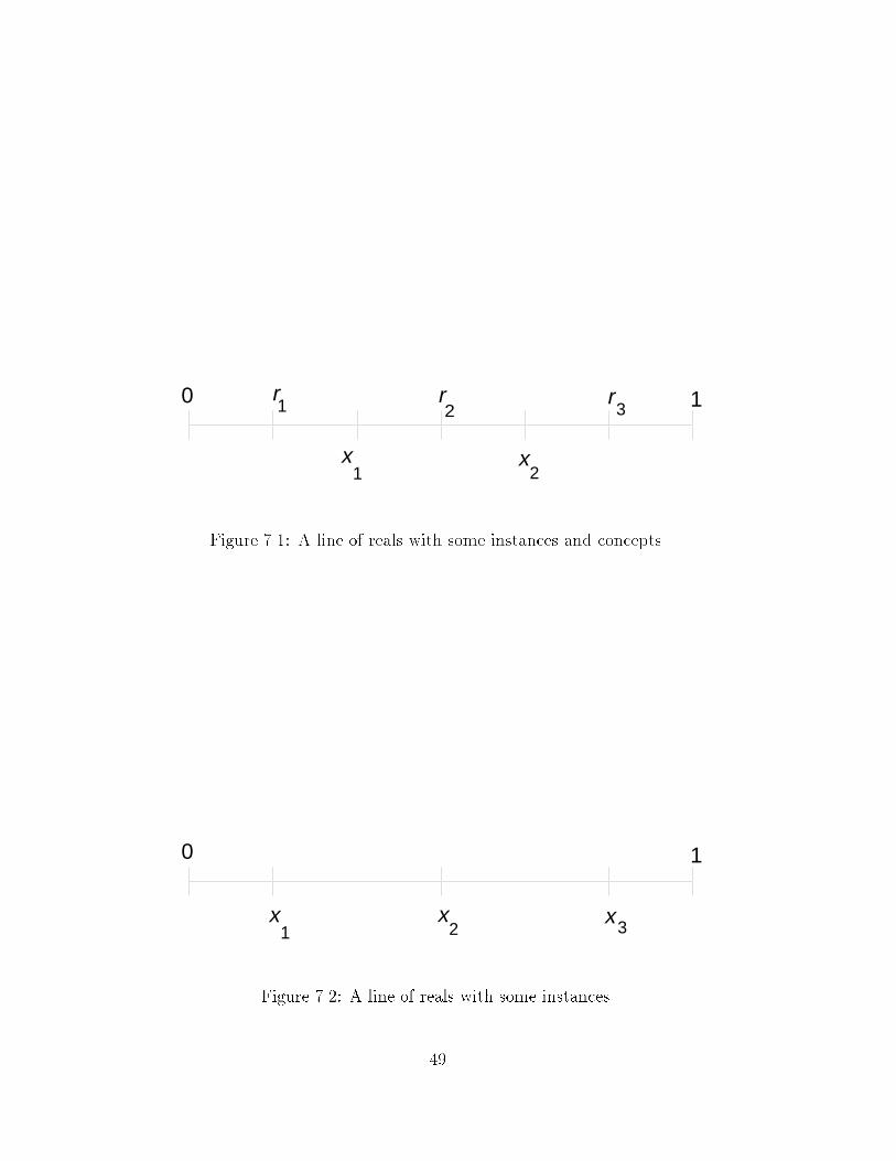
0
2x
1
x1
3r
2r1
r
Figure 7.1: A line of reals with some instances and concepts.
0
x1 2
x
1
3x
Figure 7.2: A line of reals with some instances.
49
The concepts are axis-parallel rectangles in R2. Points lying on or inside the rectangle
are positive, and points lying outside the rectangle are negative.
We �rst show that there exists a set of size four that can be shattered by C. Consider
any four points, no three of which are collinear. Clearly, these points can be shattered by
concepts from C. Finally, we must show that no set of size �ve can be shattered by C. Given
any �ve points, one of the following two cases occur.
1. At least three of the points are collinear. In this case, there is no rectangle which
contains the two extreme points, but does not contain the middle points. Thus clearly,
the �ve points cannot be shattered.
2. No three of the points are collinear. In this case, consider the bounding rectangle
formed by taking the maximum x-coordinate, maximum y-coordinate, minimum x-
coordinate, and minimum y-coordinate. Clearly, one of the �ve points (possibly more)will be contained in this bounding rectangle. Note that there is no concept containingthe points on this rectangle but not the internal points. Thus the �ve points cannotbe shattered.
Thus we have demonstrated that vcd(C) = 4.
Generalizing to axis-parallel rectangles in Rd, we get vcd(C) = 2d.
Example 7.3 Half-spaces in R2
The concepts are half-spaces in R2 formed by a line dividing R2 into two half-spaces.
Points lying in one of the half-spaces or on the dividing line are positive, and points lying inthe other half-space are negative.
We �rst show that there exists a set of size three that can be shattered by C. Considerany three non-collinear points. Clearly, they can be shattered by concepts from C. Finallywe must show that no set of size four can be shattered by C. Given any four points, one ofthe following two cases occur.
1. At least three of the points are collinear. In this case, there is no half-space whichcontains the two extreme points, but does not contain the middle points. Thus clearlythe four points cannot be shattered.
2. No three of the points are collinear. In this case, the points form a quadrilateral. Thereis no half-space which labels one pair of diagonally opposite points positive, and the
other pair of diagonally opposite points negative. Thus clearly the four points cannotbe shattered.
Thus we have demonstrated that vcd(C) = 3.
Generalizing to half-spaces in Rd, we get vcd(C) = d + 1.
Example 7.4 Closed sets in R2
50
The concepts are closed sets in R2. All points lying in the set or on the boundary of the
set are positive, and all points lying outside the set are negative.
Any set can be shattered by C. This is because the concepts can assume any shape inR2. Thus, the largest set that can be shattered by C is in�nite.
Thus, vcd(C) =1.
Example 7.5 Convex d-gons in R2
The concepts are convex polygons in R2 having d sides. All points lying in the convex
d-gon or on the sides of the convex d-gon are positive, and all points lying outside the convex
d-gon are negative.
We �rst show that there exists a set of 2d + 1 points that can be shattered. Consider
2d+1 points evenly spaced around a circle. We claim that given any labeling of these pointsone can �nd a d-gon consistent with the labeling. If there are more negative points then
use the positive points as the vertices of the d-gon. If there are more positive points use thetangents to the negative points as the edges.
Finally, we informally argue that no set of size 2d + 2 points can be shattered. If thepoints are not in a circular arrangement then clearly they can't be shattered. And if thereare in a circular arrangement switching between positive and negative points as one goesaround the circle produces a labeling that cannot be obtained by any d-gon.
So, for this concept class, vcd(C) = 2d + 1.
Generalizing to convex polygons in R2, we get vcd(C) =1.
7.4 VC Dimension and Sample Complexity
In this section, we relate the VC dimension to the sample complexity required for PAC
learning. First, we need a de�nition.
De�nition 7.6 A concept class C � 2X is trivial if C consists of one concept, or two disjointconcepts c1 and c2 such that c1 [ c2 = X.
When C is trivial, it is clear that a sample size of at most 1 is required to learn C. Nowto the more general case.
Theorem 7.1 Let C be a non-trivial, well-behaved 3 concept class.
1. C is PAC learnable if and only if the VC dimension of C is �nite 4
3This relatively benign measure-theoretic assumption holds of all the concept classes we have seen. It isdiscussed in detail in the appendix of [12].
4This assumes that the learner is limited to static sampling. It also does not consider the time or samplecomplexity of the learner.
51
2. if vcd(C) = d, where d <1, any hypothesis from C that is consistent with
m � max
2
�log
2
�;8d
�log
13
�
!
examples is �-good with probability � 1� �. The sample complexity is
O
1
�ln
1
�+vcd(C)
�ln
1
�
!:
We will not prove this theorem here. It is given in detail in Blumer et al. [12]. However,
we can note a consequence of the theorem. If vcd(C) is �nite, then C is PAC learnable with
sample size O
�1�
ln 1�
+vcd(C)
�ln 1
�
�, and if vcd(C) is in�nite, then C is not PAC learnable
at all. (See Topic 14 for a discussion of when dynamic sampling can be used to learn conceptclasses with in�nite VC dimension.)
We now describe an information-theoretic lower bound that demonstrates that the above
upper bound is almost tight.
Theorem 7.2 For any concept class C with �nite VC dimension, �nding an �-good hypoth-esis with probability � 1� � requires
1
�ln
1
�+vcd(C)
�
!
examples.
Proof: We begin by proving that �1�
ln 1�
�examples are needed.
Consider a portion of X having �-weight in the distribution DX on X. The probability
of not seeing an instance from that portion in one drawing is at most (1 � �). Thus theprobability of not seeing an instance from that portion of X in m drawings is at most(1� �)m. We want this probability to be at most �. Thus we require that
(1� �)m � �
Taking the natural logarithm of both sides, we get that
m ln (1 � �) � ln �
Dividing by ln(1� �) which is negative, gives
m �ln �
ln(1 � �)
Finally, since ln(1� �) < �� we can conclude that
m � �ln �
�
=1
�ln
1
�
52
Thus, �1�
ln 1�
�examples are needed so that we get an example from any portion of X
having �-weight with probability � (1� �).
We now want to prove that
�vcd(C)
�
�examples are needed.
Let vcd(C) = d. We shall �rst prove that additional (d) examples are needed. Then,
we will improve it to (d�).
Since vcd(C) = d, there exists a shattered set of size d. Let S = fx1; . . . ; xdg be such
a set, and let DS be a uniform distribution over S. Assume without loss of generality that
jCj = 2d.
Run the following experiment.
1. Draw sample Y = fy1; . . . ; ymg from DS where m � d2. Assume without loss of
generality that y1 = x1; y2 = x2; . . . ; ym = xm.
2. Choose target c by ipping d fair coins. (Let b1; . . . ; bd be the outcomes).
3. Run the PAC algorithm on the m pairs (x1; b1); . . . ; (xm; bm) to output hypothesis h.
4. Measure the error of h.
Consider the following modi�ed experiment.
1. Draw sample Y = fy1; . . . ; ymg from DS where m � d2. Assume without loss of
generality that y1 = x1; y2 = x2; . . . ; ym = xm.
2. Choose target c by ipping m fair coins. (Let b1; . . . ; bm be the outcomes).
3. Run the PAC algorithm on the m pairs (x1; b1); . . . ; (xm; bm) to output hypothesis h.
4. Flip d �m coins to determine the rest of c.
5. Measure the error of h.
Both the experiments have the same results. However, it is easier to measure the expectederror in the second experiment. On each point not in the sample Y , the probability of h
being correct is 12. Thus, the total expected error � (d
2)(1
2) = d
4. This implies that � and
� can no longer be chosen arbitrarily because we know that the total expected error is atleast d
4. Thus, the PAC algorithm needs at least d
2examples. This shows that we need an
additional (d) examples.
We now modify the upper bound to prove the (d�) bound. Let S0 = fx1; . . . ; xd�1g. Let
S = S0 [ fx0g and DS be the distribution on S. Let DS put weight 1� 2� on x0 and weight2�d�1
on each of x1; . . . ; xd�1. Let C 0 be the concept class obtained by taking the concepts that
shatter S0 and let x0 be positive. So jC 0j = 2d�1.
Any PAC algorithm will quickly learn that x0 is positive, but it cannot ignore S0 sincePx2S0DS(x) = 2� > �. So, the PAC algorithm must see at least half the examples in S0.
With probability 2�d�1
of seeing any of the examples in S0, the PAC algorithm would need at
53
least (d�) examples to see d
2of the examples in S0. This is because we want d
2successful
Bernoulli trials, each with 2�d�1
chance of success.
Thus combining this with the �rst part of the proof, we get that the PAC algorithm
needs
1
�ln
1
�+vcd(C)
�
!
examples to �nd an �-good hypothesis with probability at least (1� �).
7.5 Some Relations on the VC Dimension
In this section, we will see some inequalities describing the relationships between the VC
dimension of two or more concept classes, the relationships between the VC dimension of aconcept class and the size of the concept class, etc. These bounds are very useful to compute
the VC dimension of complicated concept classes that are constructed with simpler conceptclasses for which the VC dimension is known.
If C1 � C2, then clearly
vcd(C1) � vcd(C2):
Next we consider the relation between the VC dimension of C and the cardinality of C.
Given vcd(C) points, we need 2vcd(C) concepts to shatter them. Thus,
jCj � 2vcd(C)
Taking the base-2 logarithm of both sides
lg jCj � vcd(C)
For �nite C, we had earlier shown that
m �1
�
�ln jCj+ ln
1
�
�
examples were su�cient to learn C. Note that using vcd(C) instead of ln jCj gives a better
bound.
Consider the complement �C of the concept class C, de�ned as �C = fX � c : c 2 Cg. Then
vcd(�C) = vcd(C):
Consider the union of two concept classes. That is, let C = C1 [ C2 where C, C1 and C2are de�ned over the same instance space. Then,
vcd(C) � vcd(C1) + vcd(C2) + 1:
54
Consider the concept class Cs formed by the union (or intersection) of up to s concepts
from C where vcd(C) = d. For the union, Cs = f[si=1ci : ci 2 Cg, and similarly for intersec-
tion. Then, for all s � 1;vcd(Cs) � 2ds lg(3s). Thus,
vcd(Cs) = O(s ln(s)vcd(C)):
Earlier, we have de�ned �C(S) as the distinct ways that C can classify the instances in
S. We shall now bound j�C(S)j by jSj and vcd(C).
De�nition 7.7 For all d � 0;m � 0,
�d(m) =Pd
i=0
�m
i
�if m � d
= 2m otherwise
For concept class C, let vcd(C) = d and let S be a set of m distinct instances, then
j�C(S)j � �d(m):
There are some inequalities relating �d(m) using combinatorial arguments and Stirling'sapproximation.
�d(m) = �d�1(m� 1) + �d(m� 1):
For all d � 0 and m � 0,�d(m) � md + 1:
For all d � 2 and m � 2,�d(m) � md:
For all m � d � 1,
�d(m) � 2
md
d!
!��em
d
�d:
Thus, whenever vcd(C) is �nite, then �C(m) grows only polynomially in m.
55

56
CS 582T Computational Learning Theory Spring Semester, 1991
Topic 8: Representation Independent Hardness Results
Lecturer: Sally Goldman
8.1 Introduction
In Topic 3 we discussed a hardness result for learning k-term-DNF when the learner is re-
stricted to use a hypothesis class of k-term-DNF. However, we then showed that k-term-DNF
is learnable using the hypothesis class of k-CNF. While such representation-dependent hard-ness results provide some information, what one would really like to obtain is a hardnessresult for learning a concept class using any reasonable (i.e. polynomially evaluatable) hy-pothesis class. In this lecture we will brie y introduce a representation-independent hardnessresult for learning several simple concept classes such as Boolean formulas, deterministic
�nite automata, and constant-depth threshold circuits (a simpli�ed form of \neural net-works"). These hardness results are based on assumptions regarding the intractability ofvarious cryptographic schemes such as factoring Blum integers and breaking the RSA func-tion. The material presented here is just a brief introduction to the paper, \CryptographicLimitations on Learning Boolean Formulae and Finite Automata," by Michael Kearns and
Leslie Valiant [26]. We only give the intuition behind the hardness results|no details aredescribed here. For the complete proofs we refer to reader to the Kearns and Valiant pa-per. Also a more complete discussion of these results is contained in Chapter 7 of Kearns'thesis [27].
8.2 Previous Work
Before describing the results of Kearns and Valiant we �rst brie y review the only previ-
ously known representation-independent hardness result. This previous result follows fromthe work of Goldreich, Goldwasser and Micali [19]. Let cktp(n)n denote the class of Boolean
circuits over n inputs with at most p(n) gates and let cktp(n) =Sn�1ckt
p(n)n . Goldreich,
Goldwasser, and Micali showed that if there exists a one-way function, then for some polyno-
mial p(n), cktp(n) is not polynomially learnable by any polynomially evaluatable hypothesis
class.
Observe that the most powerful (polynomially evaluatable) hypothesis that can be output
by any polynomial-time learning algorithm is a hypothesis that is itself a polynomial-timealgorithm (or equivalently a polynomial-size Boolean circuit). Thus we cannot �nd e�cient
learning algorithms for concept classes that do not have small circuits|no learning algorithm
even has time to just write down the representation. Schapire [37] has formally shownthat any representation class that is not polynomially evaluatable cannot be learned in
57
polynomial time. With this in mind, observe that the result of Goldreich, et al. shows that
not everything with a small representation is e�ciently learnable (assuming the existence
of one-way functions). However, there is a large gap between the computational power of
cktp(n) and the classes for which we have e�cient learning algorithms. Thus we would like
to prove representation-independent hardness results for less powerful concept class such as
the classes of Boolean formulas.
8.3 Intuition
In this section we describe the intuition behind the hardness results of Kearns and Valiant.
We begin by very informally describing the type of cryptographic scheme on which this
hardness result is based.
Suppose that Alice and Bob wish to communicate privately inspite of an eavesdropperEve who has bugged the communication line between Alice and Bob. (We make no as-sumptions about Eve except that she has a polynomial bound on her computing resources.)Furthermore, we want a scheme which does not require Alice and Bob to meet privately
ahead of time to set up their encoding scheme. Such encryption scheme can be devisedusing a trapdoor function. Informally, a trapdoor function is one that can be computedin polynomial time (i.e., it is easy to compute f(x) on input x) but cannot be inverted inpolynomial time (i.e., it is hard to compute x on input f(x)) unless one is the \creator"of the function and thus possesses a piece of \trapdoor" information that makes inversion
possible in polynomial time.Cryptographic schemes based on such trapdoor functions are known as public-key cryp-
tographic systems. In such a scheme each user creates a trapdoor function f and publishesa program for computing f . (This program must reveal no information about f�1.) Thenanyone can send messages to the given user over the nonsecure communication line and onlythat user can decode such messages. So Alice and Bob can communicate with each other
using such a scheme where they have both created their own trapdoor function. We say thatthis system is secure if Eve cannot do noticeably better than random guessing in trying todecode a bit that has been encoded using this encryption scheme. More formally, if
Pr[Eve predicts correct decoded bit] �1
2+
1
p(n)
for some polynomial p(n) then the system is not secure.
We now describe how we can use the existence of such a public-key cryptographic system,such as RSA, to obtain a representation-independent hardness result for learning. For the
hardness result view Eve as a learning algorithm. Since a program for f is available she
can create any polynomially number of pairs of the form (f(x); x) that she likes by simply
choosing x and then computing f(x). If we set y = f(x) observe that such pairs have
the form (y; f�1(y)) and thus can be viewed as labeled examples of f�1. Thus public-key cryptography assumes the existence of functions that are not learnable from examples.
In fact, unlike the PAC learning model in which we ask the learner to be able to make
58
arbitrarily good predications, in the cryptographic scheme we only ask the learner, Eve, to
make predictions that are noticeably better than random guessing. (This \weak learning"
model will be discussed further in the next topic.)
Observe that in the learning problem described above f�1 is \simple" in the sense that
it has a small circuit (determined by the trapdoor used for decoding.) So the theory of
cryptography provides simple functions that are di�cult to learn. Kearns and Valiant show
how to re�ne the functions provided by cryptography to �nd the simplest functions that
are di�cult to learn. Using this basic approach (of course, with lots of details which we
will not discuss here) they show that polynomial-sized Boolean formulas, and constant-
depth threshold circuits are not even weakly learnable by any polynomially evaluatable
hypothesis class. Then using a prediction-preserving reduction (described below) of Pitt and
Warmuth [34] it follows that deterministic �nite automata are also not learnable.
8.4 Prediction Preserving Reductions
Given that we now have a representation-independent hardness result (assuming the securityof the various cryptographic schemes) one would like a \simple" way to prove that otherproblems are hard in a similar fashion as one proves a desired algorithm is intractable byreducing a known NP-complete problem to it. Such a complexity theory for predictability
has been provided by Pitt and Warmuth [34]. They formally de�ne a prediction-preservingreduction (A � B) that enables a prediction algorithm for concepts of type B to solve aprediction problem for concepts of type A. This reduction consists of the following twomapping:
1. A polynomial time computable function f that maps unlabeled examples of A tounlabeled examples of B.
2. A function g that maps representations of A to representations of B. Furthermore,this mapping g need not be computable|it is only required to be length preservingwithin a polynomial.
Then given a polynomial prediction algorithm for concepts of type B one can use it toobtain a polynomial prediction algorithm for concepts of typeA in the obvious manner. Thus
if A is known not to be learnable then B also cannot be learnable. They describe several suchreductions in their paper, one of which is a reduction from Boolean formula predictability to
DFA predictability (Boolean formula � DFA). Thus since Kearns and Valiant have shownthat Boolean formula are not predictable (under cryptographic assumptions) it immediately
follows that DFA are not predictable.
59

60
CS 582T Computational Learning Theory Spring Semester, 1991
Topic 9: Weak Learning
Lecturer: Sally Goldman Scribe: Andy Fingerhut
9.1 Introduction
In the �rst lecture we introduced the probably approximately correct (PAC) or distribution
free model of learning. In this model, the learner is presented with examples which are
randomly and independently drawn from an unknown but �xed distribution. The learnermust, with arbitrarily high probability, produce a hypothesis that is arbitrarily close to thetarget concept.
As we saw in the last lecture, the representation-independent hardness results based onthe security of various cryptographic schemes motivated the study of learning algorithms
which do not attain arbitrarily high accuracy, but do just slightly better than random guess-ing (by an inverse polynomial in the size of the problem). This leads to the notion of weaklearning which is the subject of this lecture. In particular we describe an algorithm to con-vert any weak learning algorithm into a PAC-learning algorithm. The material presentedhere comes from the paper, \The Strength of Weak Learnability," by Robert Schapire [37].
9.2 Preliminaries
We begin by formally de�ning the weak learning model. As in the PAC model, for a given sizeparameter n, there is a set of instances Xn. A concept c is a Boolean function c : Xn ! f0; 1g.A concept class Cn � 2Xn is a set of concepts. The learner has access to a source EX of
labeled examples. Each time EX is called, an example is drawn randomly and independentlyaccording to a �xed but unknown distribution D on Xn, and returned in unit time.
After drawing some examples and running for a time, the learning algorithm must output
an hypothesis h. This is a polynomially (in n) evaluatable hypothesis which, when given aninstance v 2 Xn, returns a prediction. The hypothesis may be randomized (this is important
for weak learning).
We write Prob[�(v)] to denote the probability that the predicate � holds for a particular
instance v. This probability may be between 0 and 1 because of randomness in evaluating
�(v). For example, think of �(v) as the event that h(v) = 1 for some randomized hypothesis
h. By Probv2D[�(v)] we denote the probability that, after drawing v randomly from distri-bution D, �(v) holds. Thus, assuming that these two random events (i.e., choice of v and
evaluation of �(v)) are independent, we have Probv2D[�(v)] =P
v2XnD(v)Prob[�(v)] where
D(v) denotes the probability of instance v being chosen under distribution D.
61
Finally, we can de�ne the error of an hypothesis h on c under distribution D as
errorD(h) = Probv2D[h(v) 6= c(v)]:
If the errorD(h) � �, we say h is �-close to c under D. The accuracy of h is one minus its
error.
We say that a concept class C is strongly learnable (called simply learnable or PAC-
learnable elsewhere) if there is an algorithm A such that, for all n � 1, for all target concepts
c 2 Cn, for all distributions D and parameters 0 < �; � � 1, algorithm A, given n, �, �, and
access to oracle EX, outputs a hypothesis h such that, with probability � 1 � �, errorD(h)
is at most �. Algorithm A should run in time polynomial in n, 1=�, and 1=�.
To be weakly learnable, there must be a polynomial p in addition to the algorithm A such
that, for all n � 1, c 2 Cn, for all distributions D, and for all 0 < � � 1, algorithm A, given
n, �, and access to oracle EX, outputs a hypothesis h such that, with probability � 1 � �,errorD(h) is at most (1=2 � 1=p(n)). Algorithm A should run in time polynomial in n and1=�.
9.3 The Equivalence of Strong and Weak Learning
It should be clear that if C is strongly learnable, then it is weakly learnable|just �x � = 1=4(or any constant less than 1=2.) The converse (weak learnability implying strong learnability)is not at all obvious. In fact, if one restricts the distributions under which the weak learningalgorithm runs then weak learnability does not imply strong learnability. In particular,Kearns and Valiant [26] have shown that under a uniform distribution monotone Boolean
functions are weakly, but not strongly, learnable. Thus it will be important to take advantageof the requirement that the weak learning algorithm must work for all distributions. Theremainder of this section will be devoted to proving the main result of these notes.
Theorem 9.1 If concept class C is weakly learnable, then it is strongly learnable.
Note that weak learning, even though it may be \weak", is not necessarily easy to do.Consider the simple-minded algorithm which draws and memorizes a polynomial q(n; 1=�)
number of examples. It then outputs a hypothesis h which looks up known results and oth-
erwise ips a fair coin to determine the answer. Suppose that jXnj = 2n and the distributionD is the uniform distribution. Then the errorD(h) = (1=2 � q(n; 1=�)=2n), which is larger
than (1=2� 1=p(n)) for any polynomial p. Thus it is non-trivial to devise an algorithm thatweakly learns a concept class.
9.3.1 Hypothesis Boosting
Proving that weak learnability implies strong learnability has also been called the hypothesis
boosting problem, because a way must be found to boost the accuracy of slightly-better-than-half hypotheses to be arbitrarily close to 1.
62
Suppose that we have a learning algorithm A which produces hypotheses with error at
most � (for � < 1=2). Simply running A twice to produce hypotheses h1 and h2 may not
help at all|they may err in a very similar way in their classi�cation. After obtaining h1, we
need a way to force the next hypothesis output to be more accurate. The answer lies in the
power of A to work given any distribution D on the instances. If we give A a distribution
D0 such that the error of h1 is exactly 1=2, then the hypothesis h2 produced must have an
error � � on it, which means that h2 has learned something about the target concept which
h1 did not. Unfortunately, the probability that h1 and h2 classify a random instance the
same (their \overlap") may be very low; in this case, it would seem that h1 and h2 learned
almost completely di�erent parts of the D. To handle this, we ask A to learn a \tie-breaker"
hypothesis h3. This time, A is given a distribution D00 on the instances on which h1 and h2disagree.
Thus to improve the accuracy of the weak learning algorithm A, the algorithm A0 sim-ulates A on distributions D;D0, and D00 and outputs a hypothesis that takes the majorityvote of the three hypothesis obtained. Of course, algorithm A0 must use D to simulate thedistributions D0 and D00. We now describe how this task is achieved. These two modi�eddistributions are created by �ltering the original distribution. In other words, A0 will drawsamples from D and discard undesirable samples to obtain the desired distribution. Whilethis requires additional samples (thus increasing both the time and sample complexity) itcan be made to run in polynomial time. The key observation is that we will only apply the�lter if the probability of obtaining an example which passes through the �lter is (�). Thedistribution D0 given to learn h2 is produced by the procedure EX2 de�ned below. Likewise,the distribution D00 for learning h3 is produced by EX3.
EX2(EX ; h1)
ip fair coin
if heads then return the �rst instance v from EX for which h1(v) = c(v)
else return the �rst instance v from EX for which h1(v) 6= c(v)
EX3(EX ; h1; h2)
return the �rst instance v from EX for which h1(v) 6= h2(v)
Thus we can now formally state the hypothesis boosting procedure as follows:
1. Run the weak learning algorithm using EX. Let h1 be the hypothesis output.
2. Run the weak learning algorithm using EX2(EX;h1). Let h2 be the hypothesis output.
3. Run the weak learning algorithm using EX2(EX;h1; h2). Let h3 be the hypothesisoutput.
4. Return h = majority(h1; h2; h3).
An important question to address is: How much better is the accuracy of h than theaccuracy of h1? Suppose that the given weak learning algorithm is guaranteed to output a
63
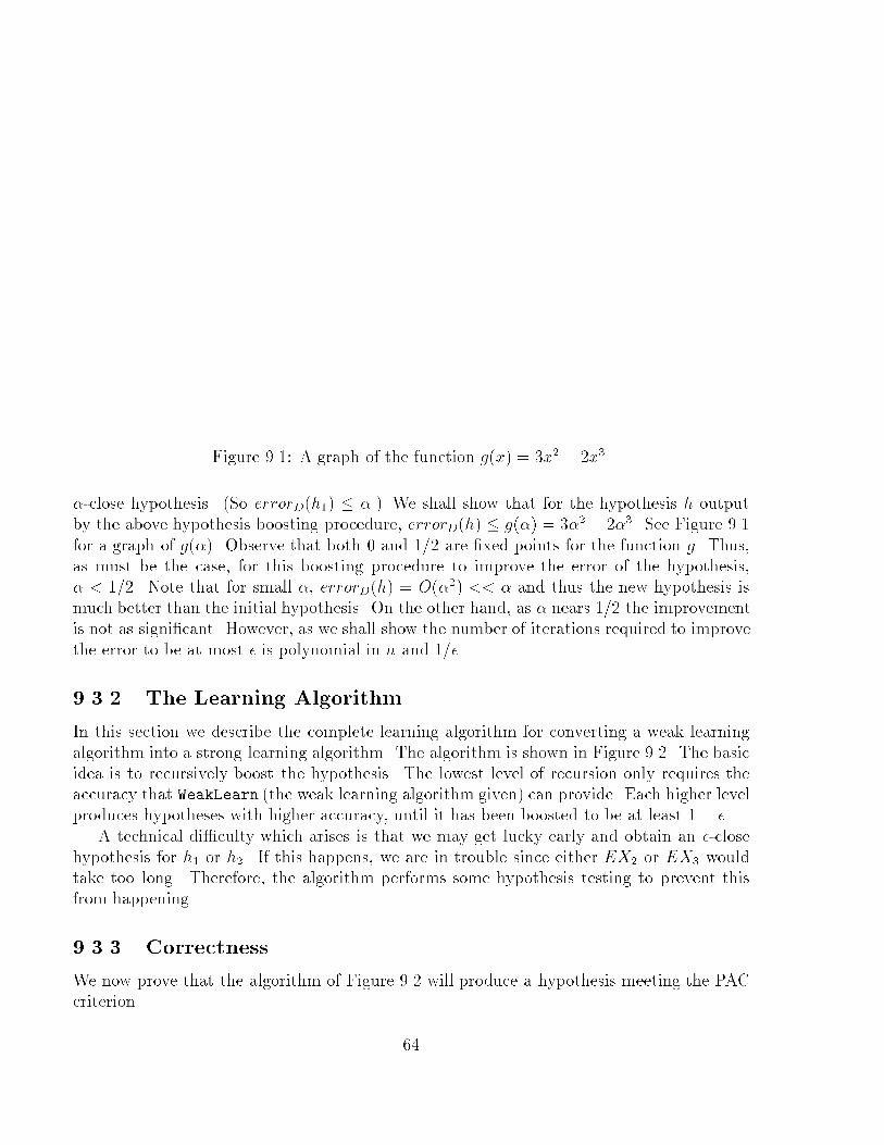
Figure 9.1: A graph of the function g(x) = 3x2 � 2x3.
�-close hypothesis. (So errorD(h1) � �.) We shall show that for the hypothesis h outputby the above hypothesis boosting procedure, errorD(h) � g(�) = 3�2 � 2�3. See Figure 9.1
for a graph of g(�). Observe that both 0 and 1=2 are �xed points for the function g. Thus,as must be the case, for this boosting procedure to improve the error of the hypothesis,� < 1=2. Note that for small �, errorD(h) = O(�2) << � and thus the new hypothesis ismuch better than the initial hypothesis. On the other hand, as � nears 1=2 the improvementis not as signi�cant. However, as we shall show the number of iterations required to improve
the error to be at most � is polynomial in n and 1=�.
9.3.2 The Learning Algorithm
In this section we describe the complete learning algorithm for converting a weak learningalgorithm into a strong learning algorithm. The algorithm is shown in Figure 9.2. The basic
idea is to recursively boost the hypothesis. The lowest level of recursion only requires the
accuracy that WeakLearn (the weak learning algorithm given) can provide. Each higher levelproduces hypotheses with higher accuracy, until it has been boosted to be at least 1 � �.
A technical di�culty which arises is that we may get lucky early and obtain an �-closehypothesis for h1 or h2. If this happens, we are in trouble since either EX2 or EX3 would
take too long. Therefore, the algorithm performs some hypothesis testing to prevent thisfrom happening.
9.3.3 Correctness
We now prove that the algorithm of Figure 9.2 will produce a hypothesis meeting the PAC
criterion.
64
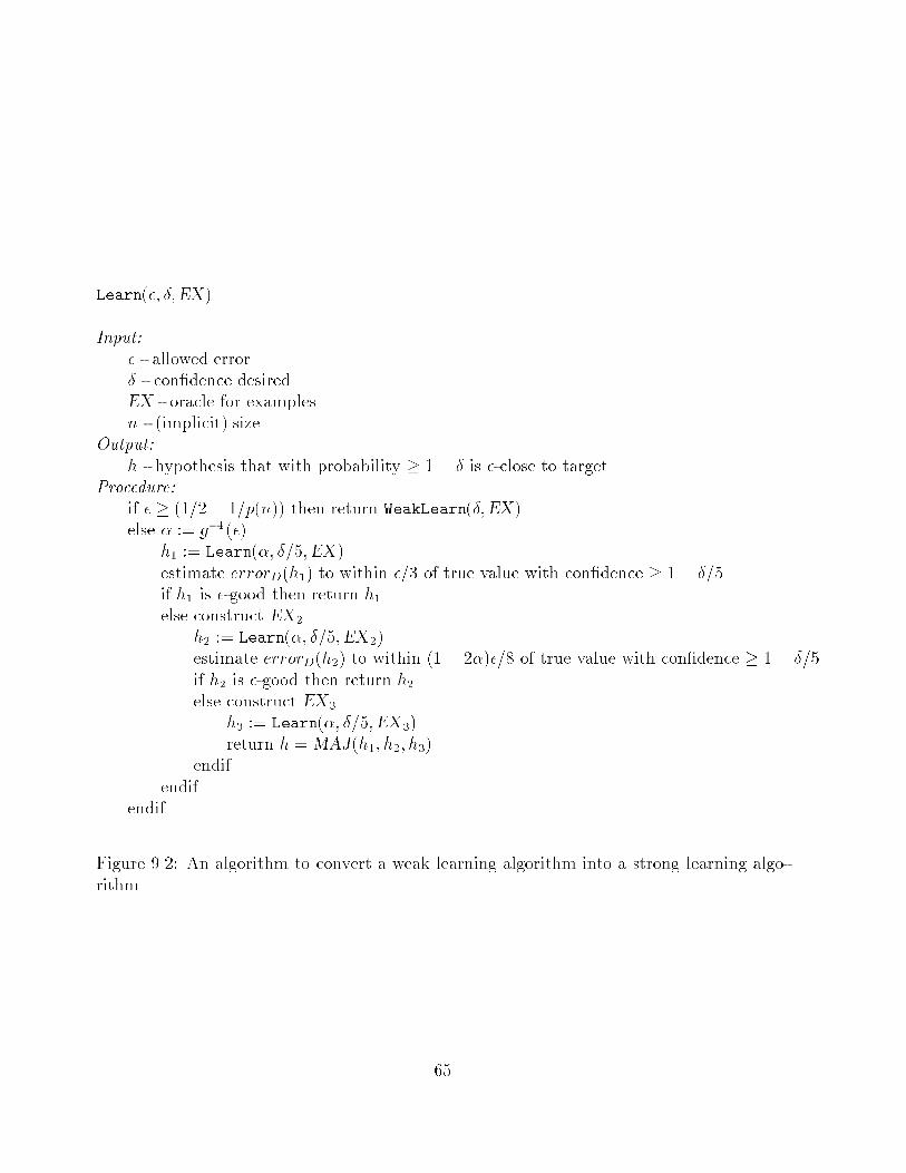
Learn(�; �;EX)
Input:
� - allowed error
� - con�dence desired
EX - oracle for examplesn - (implicit) size
Output:
h - hypothesis that with probability � 1 � � is �-close to targetProcedure:
if � � (1=2 � 1=p(n)) then return WeakLearn(�;EX)else � := g�1(�)
h1 := Learn(�; �=5;EX)
estimate errorD(h1) to within �=3 of true value with con�dence � 1� �=5if h1 is �-good then return h1else construct EX2
h2 := Learn(�; �=5;EX2)estimate errorD(h2) to within (1� 2�)�=8 of true value with con�dence � 1 � �=5if h2 is �-good then return h2else construct EX3
h3 := Learn(�; �=5;EX3)return h = MAJ(h1; h2; h3)
endif
endif
endif
Figure 9.2: An algorithm to convert a weak learning algorithm into a strong learning algo-
rithm.
65
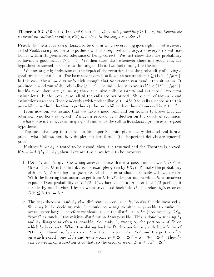
Theorem 9.2 If 0 < � < 1=2 and 0 < � � 1, then with probability � 1 � �, the hypothesis
returned by calling Learn(�; �;EX) is �-close to the target c under D.
Proof: De�ne a good run of Learn to be one in which everything goes right. That is, every
call of WeakLearn produces a hypothesis with the required accuracy, and every error estima-
tion is within its prescribed tolerance of being correct. We �rst show that the probability
of having a good run is � 1 � �. We then show that whenever there is a good run, the
hypothesis returned is �-close to the target. These two facts imply the theorem.
We now argue by induction on the depth of the recursion that the probability of having a
good run is at least 1��. The base case is depth = 0, which occurs when � � (1=2�1=p(n)).
In this case, the allowed error is high enough that WeakLearn can handle the situation. It
produces a good run with probability� 1��. The induction step occurs if � < (1=2�1=p(n)).
In this case, there are (at most) three recursive calls to Learn and (at most) two error
estimations. In the worst case, all of the calls are performed. Since each of the calls andestimations succeeds (independently) with probability � 1� �=5 (the calls succeed with this
probability by the induction hypothesis), the probability that they all succeed is � 1 � �.From now on, we assume that we have a good run, and our goal is to prove that the
returned hypothesis is �-good. We again proceed by induction on the depth of recursion.
The base case is trivial, assuming a good run, since the call to WeakLearn produces an �-goodhypothesis.
The inductive step is trickier. In his paper Schapire gives a very detailed and formal
proof|what follows here is a simpler but less formal (i.e. important details are ignored)proof.
If either h1 or h2 is tested to be �-good, then it is returned and the Theorem is proved.
If h = MAJ(h1; h2; h3), then there are two cases for h to be incorrect.
1. Both h1 and h2 give the wrong answer. Since this is a good run, errorD0(h2) � �.(Recall that D0 is the distribution of examples given by EX2). To make the probabilityof h1 = h2 6= c as high as possible, all of this error should coincide with h1's error.With the �ltering that occurs to get from D to D0, the portion on which h1 is incorrect
expands from probability � to 1=2. If h2 has all of its error on that 1=2 portion, it
shrinks by multiplying it by 2� when translated back into D. Therefore h2's error onD is � 2�(�) = 2�2.
2. The hypotheses h1 and h2 give di�erent answers, and h3 breaks the tie incorrectly.
Since h3 is the deciding vote, it should be wrong as often as possible to make the
overall error large. Therefore we should make the distribution D00 (produced by EX3)\cover" as much of the original distribution D as possible. This is done by making h1and h2 disagree as often as possible. So, make h2 wrong on the portion � of D0 onwhich h1 is correct. When translating back to D, this portion expands by a factor of
2(1� �). Therefore, h2's error on D is � 2(1��)� = 2�� 2�2, and the portion of D
on which exactly one of h1 and h2 is wrong is � 2� � 2�2 + � = 3� � 2�2. Thus h3can be wrong on a fraction � of that, so the error of h3 on D is � 3�2 � 2�3.
66
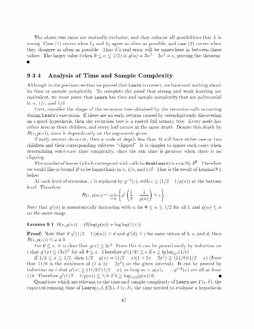
The above two cases are mutually exclusive, and they exhaust all possibilities that h is
wrong. Case (1) covers when h1 and h2 agree as often as possible, and case (2) covers when
they disagree as often as possible. Thus h's real error will be somewhere in between these
values. The larger value (when 0 � � � 1=2) is g(�) = 3�2 � 2�3 = �, proving the theorem.
9.3.4 Analysis of Time and Sample Complexity
Although in the previous section we proved that Learn is correct, we have said nothing about
its time or sample complexity. To complete the proof that strong and weak learning are
equivalent, we must prove that Learn has time and sample complexity that are polynomial
in n, 1=�, and 1=�.
First, consider the shape of the recursion tree obtained by the recursive calls occurringduring Learn's execution. If there are no early returns caused by serendipitously discoveringan �-good hypothesis, then the recursion tree is a rooted full ternary tree. Every node has
either zero or three children, and every leaf occurs at the same depth. Denote this depth byB(�; p(n)), since it depends only on the arguments given.
If early returns do occur, then a node at depth less than B will have either one or twochildren and their corresponding subtrees \clipped". It is simpler to ignore such cases whendetermining worst-case time complexity, since the run time is greatest when there is no
clipping.The number of leaves (which correspond with calls to WeakLearn) is exactly 3B. Therefore
we would like to bound B to be logarithmic in n, 1=�, and 1=�. That is the result of Lemma 9.1below.
At each level of recursion, � is replaced by g�1(�), with � � (1=2� 1=p(n)) at the bottom
level. Therefore
B(�; p(n)) = mini�0
(gi
1
2�
1
p(n)
!� �
):
Note that gi(�) is monotonically increasing with � for 0 � � � 1=2 for all i, and g(�) � �
on the same range.
Lemma 9.1 B(�; p(n)) = O(log(p(n)) + log log(1=�))
Proof: Note that if gb(1=2 � 1=p(n)) � d and gc(d) � � for some values of b, c, and d, then
B(�; p(n)) � a+ b.For 0 � x, it is clear that g(x) � 3x2. From this it can be proved easily by induction on
i that gi(x) � (3x)2i
for all 0 � x. Therefore gc(1=4) � � if c � lg log4=3(1=�).
If 1=4 � x � 1=2, then 1=2 � g(x) = (1=2 � x)(1 + 2x � 2x2) � (11=8)(1=2 � x) (Note
that 11=8 is the minimum of (1 + 2x � 2x2) on the given interval). It can be proved byinduction on i that gi(x) � (11=8)i(1=2 � x), as long as x, g(x), . . . , gi�1(x) are all at least1=4. Therefore gb(1=2 � 1=p(n)) � 1=4 if b � log11=8(p(n)=4).
Quantities which are relevant to the time and sample complexity of Learn are T (�; �), theexpected running time of Learn(�; �;EX), U(�; �), the time needed to evaluate a hypothesis
67
returned by Learn, and M(�; �), the expected number of samples needed by Learn. There are
corresponding quantities t(�), u(�), and m(�) for WeakLearn(�;EX). All of these functions
also depend (implicitly) on n.
These functions can be bounded quite e�ectively by the use of recurrence relations. These
recurrences can be obtained by examination of Learn, with the base case being WeakLearn
and its complexity. The �nal results will be mentioned here as lemmas, with proofs omitted.
See Schapire's paper for the complete proofs.
Lemma 9.2 The time to evaluate a hypothesis returned by Learn(�; �;EX) is U(�; �) =
O(3B � u(�=5B).
Lemma 9.3 Let r be the expected number of examples drawn from EX by any oracle EX i
simulated by Learn on a good run when asked to provide a single example. Then r � 4=�.
Lemma 9.4 On a good run, the expected number of examplesM(�; �) needed by Learn(�; �;EX)is
O
36B
�2� (p2 log(5B=�) +m(�=5B))
!
Lemma 9.5 On a good run, the expected execution time of Learn(�; �;EX) is given by
T (�; �) = O
3B � t(�=5B) +
108B � u(�=5B)
�2� (p2 log(5B=�) +m(�=5B))
!
The fact that nearly all of the expected values above are only taken over good runs ofLearn can be taken into account by \borrowing" some of the con�dence � for that purpose.
9.4 Consequences of Equivalence
There are many very interesting consequences that follow from this main result (Theorem 9.1.We shall just brie y mention a few here. We refer the reader to Schapire's paper for moredetails on these consequences and a discussion of other interesting corollaries.
One of the more notable corollaries of Theorem 9.1 is a partial converse of Occam's Razor(see Topic 6). That is, if a concept class is learnable, then any sample can be compressed with
high probability. More speci�cally, if C is PAC learnable then there exists a polynomial time
algorithm which with con�dence 1� � outputs a consistent hypothesis of size polynomial inn and =logm for any sample of size m labeled according to a concept c=inC. This corollaryleads to the result that any representation class that is not polynomially evaluatable cannot
be learned in polynomial.
Another interesting result discussed is an improved version of the learning algorithm given
here, which achieves asymptotic performance which is poly-logarithmic in terms of 1=�. Thus
using this improved version of Learn an existing strong learning algorithm performance canbe made to be poly-logarithmic in terms of 1� by �rst �xing the error of the given strong
learning algorithm at, say, � = 1=4 to obtain a weak learning algorithm. Then use this
improved version of Learn to convert the weak learning algorithm back into a strong learning
algorithm.
68
CS 582T Computational Learning Theory Spring Semester, 1991
Topic 10: Learning With Queries
Lecturer: Sally Goldman Scribe: Kevin Ruland
10.1 Introduction
In these notes we study the model of learning with queries. The material presented in this
lecture comes from the paper, \Queries and Concept Learning," by Dana Angluin [3]. In the
model of learning with queries, the learner must identify an unknown hypothesis L� from
some countable concept space of subsets of a universal set of instances. Unlike in the PACmodel, the algorithm is not given a stochastically generated sequence of labeled instances.It is instead allowed to actively explore its environment by asking questions of an oracle.
Throughout these notes we use the following notation.
� C = fL1; L2; . . .g is the set of concepts
� L� is the target concept
� U is the instance space
Angluin [3] de�nes many di�erent kinds of queries. We now de�ne the types of querieswe will consider here.
Membership Query The oracle will respond to input x 2 U \yes" if x 2 L�, otherwise itreplies \no".
Equivalence Query The oracle will respond to input hypothesis h 2 C \yes" if h = L�,
otherwise it will return some counterexample x 2 h�L�. The counterexample returned
by the oracle is selected by an all-powerful adversary, and no assumptions can be madeabout it.
Restricted Equivalence Query The oracle will respond to input hypothesis h 2 C \yes"if h = L�, otherwise it responds \no." It does not return a counterexample.
Generalized Equivalence Query The oracle will respond as an equivalence query to any
input hypothesis that is a subset of U .
Unlike the PAC model in which the learner need only output a hypothesis that is a good
approximation to the target concept, in the model of learning with queries, the learner mustachieve exact identi�cation. We say an algorithm exactly identi�es the target concept L�with access to certain types of queries if it always halts and outputs a concept equivalent toL�. That is, for each element of x 2 U the concept output classi�es x as L� does.
69
10.2 General Learning Algorithms
In this section we explore some generic algorithms for learning with membership and equiv-
alence queries. Then in the next section, we explore the relationship between this learning
model and the PAC model. Finally, we will consider learning algorithms for particular
concept classes.
10.2.1 Exhaustive Search
The most trivial algorithm that uses only equivalence queries is exhaustive search where
each concept in C is tried in turn until the correct hypothesis is found. This method clearly
requires, in the worst case, jCj � 1 equivalence queries. It is interesting to note that for
some classes this algorithm is no worse than any other. For example, consider the singletons,
where for �xed instance space U , C = f fxg j x 2 U g. In this class, an adversary can respond
to an equivalence query by returning the element in the hypothesis as the counterexample.This strategy allows the learner to eliminate at most one concept for each equivalence query.Also, C even requires jCj � 1 membership queries because the adversary could reply \no" toeach query.
This observation is generalized in the following lemma.
Lemma 10.1 Suppose C = fL1; . . . ; LNg, and there exists a set L\ =2 C such that
Li \ Lj = L\; i 6= j
Then any algorithm that achieves exact identi�cation for any L� 2 C must make at leastN � 1 equivalence and membership queries in the worst case.
Proof: We must exhibit an adversary which answers each query in such a way that only
a single concept can be eliminated. Keep in mind that the adversary can choose the targetconcept as the learning session progresses. Namely, the adversary will keep a list of targetconcepts that are consistent with all previous queries. The learner cannot achieve exactidenti�cation until only one concept remains in the adversary's list.
For a membership query on instance x, if x 2 L\ then reply \yes," otherwise reply \no."
In the �rst case, no concepts from the adversary's list are eliminated because x is in everyconcept. In the second, at most one concept, the concept containing x, is eliminated|if two
were eliminated, Li and Lj, then Li \ Lj � L\ [ fxg, a contradiction.For an equivalence query on hypothesis L 6= L�, reply \no" and return any x 2 L \ L\.
Such an x exists since L\ =2 C, so L\L\ 6= ;. Also, if x 2 L\ then no concepts are eliminated,
and if x =2 L\ then at most one concept is eliminated.There is a dual result for union.
10.2.2 The Halving Algorithm
If the learner is allowed a more powerful equivalence query, better results are obtainable.Recall that the generalized equivalence query is similar to the equivalence query but allows
70
as input any subset of U . Using such a query, any �nite concept class can be learned in no
more than blg jCjc queries using the following algorithm.
Halving Algorithm(C)If C contains one element L, then L = L�. Halt.
Else
Let MC = fx j x 2 C for at least jCj
2concepts g.
Make generalized equivalence query with hypothesis MC
If \yes" then MC is equivalent to L�. Halt and output MC.
Else let x be the counterexample.
If x 2MC then C0 = C n fL 2 C j x 2 L gElse C0 = fL 2 C j x 2 L gHalving Algorithm(C0)
Theorem 10.1 The number of queries performed by the halving algorithm is at most blg jCjc.
Proof: A query is made if jCj > 1 and every query eliminates at least half of the concepts.
The upper bound is often not tight. For example, for the class of singletons the halvingalgorithm makes only one mistake versus the upper bound of lg n given in Theorem 10.1.Littlestone [29] gives an algorithm whose performance on any class is shown to be optimal.(This algorithm is discussed in Topic 12.)
A major drawback of the halving algorithm is that it is often not computationally
feasible|often exponential computation time is needed to construct MC. However, it cansometimes be e�ciently implemented. As an example note that Valiant's algorithm forlearning k-CNF [43] indirectly implements the halving algorithm. Let h be de�ned as theconjunction of all clauses that have been true in all counterexamples. (Recall that if h � L�,then h is consistent with all negative examples and thus for any counterexample x to h,L�(x) = +.) Now let C0 = f concepts consistent with all counterexamples g, so C0 consists of
every k-CNF formula that is a conjunction of some subset of the clauses in h. The hypothesesh constructed in this manner predicts according to the halving algorithm. If for a particularinstance all clauses in h are true, the majority is true. Similarly, if for an instance some
clause l in h is false, for every L 2 C0 that is true, there is some other hypothesis, L0 2 C0
(namely L ^ l), that is false. So, if ties are false, the majority is false.
See Topic 20 for a discussion on how approximate counting schemes can be used toe�ciently implement a variant of the halving algorithm.
10.3 Relationship Between Exact Identi�cation and
PAC Learnability
In this section we describe how an algorithm that uses equivalence queries can be convertedto a PAC-learning algorithm. We then give an example to demonstrate the converse is not
true.
71
Theorem 10.2 Any algorithm that uses equivalence queries to achieve exact identi�cation
can be modi�ed to achieve the PAC criterion (i.e., Pr[error(h) � �] � �) using calls to EX
instead of equivalence queries. Furthermore, if the algorithm for learning with equivalence
queries runs in polynomial time, then so will the PAC-learning algorithm.
Proof: We need to simulate an equivalence query with calls to EX. For the ith equivalence
query, make qi =l1�(ln 1
�+ i ln 2)
mcalls to EX. If hi (the ith hypothesis) is not consistent
with a particular example, then that is the counterexample. Given that hi is consistent with
all qi examples,
Pr[error(hi) > �] � (1� �)qi
Let h be the �nal hypothesis. So
Pr[error(h) > �] �1Xi=1
(1� �)qi
�1Xi=1
e��qi
�1Xi=1
�
2i
= �
where the second inequality holds because for all x, 1 � x � e�x. Finally, observe that thenumber of calls to EX made by the simulation is polynomial in the number of equivalencequeries made by the original algorithm.
One can consider a variation of the PAC model in which the learner can either askfor a random example from EX or ask a membership query. We say a concept class is
PAC-learnable with membership queries if the leaner can meet the PAC-criterion using apolynomial number of calls to EX and polynomial number of membership queries. As animmediate corollary to the above theorem we obtain.
Corollary 10.1 A concept class that is learnable with equivalence and membership queries
is PAC learnable with membership queries. Furthermore, if the algorithm for learning with
equivalence and membership queries uses polynomial time, then so will the PAC-learningalgorithm.
The converse to the preceding theorem is false if e�ciency must be preserved. Consider
the class of singletons de�ned on the instance space of all binary strings of length n. We
have already seen that the class of singletons requires jCj � 1 = 2n � 1 equivalence queries,
but it only requiresl1�(n ln 2 � ln �)
mcalls to EX in the PAC model.
10.4 Examples of Exactly Identi�able Classes
In this section we will exhibit examples, some with proofs, of classes that can be exactlyidenti�ed by membership and equivalence queries.
72
10.4.1 k-CNF and k-DNF Formulas
As we saw in the last section, Valiant's algorithm for learning k-CNF can be used to e�-
ciently implement the halving algorithm. Thus it follows that this class is learnable using
a polynomial number of equivalence queries. There is a logically dual method for k-DNF
formulas. Littlestone [29] describes an algorithm for learning these classes that may use
signi�cantly fewer queries. (This algorithm is described in the notes for Topic 12.) Fi-
nally, we note that by applying Lemma 10.1 to the class of 1-CNF formulas one gets that
2n�1 restricted equivalence and membership queries are needed in the worst case. A similar
hardness result can be obtained for 1-DNF.
10.4.2 Monotone DNF Formulas
In this section we describe an e�cient algorithm for learning any monotone DNF formulausing membership and equivalence queries.
Theorem 10.3 The class of monotone DNF formulas over n variables is exactly identi�ableby equivalence and membership queries in time polynomial in n and the number of terms inthe target concept.
Before we prove this we give a de�nition and some observations.
De�nition 10.1 A prime implicant t of a propositional formula � is a satis�able product ofliterals such that t implies � but no proper subterm of t implies �.
Example 10.1 � = ac _ b�c has prime implicants ac, b�c, and ab.
The number of prime implicants of a general DNF formula may be exponentially largerthan the number of terms in the formula. However, for monotone DNF, the number of primeimplicants is not greater than the number of terms in the formula.
Proof: [of Theorem 10.3] In the following let fy1; y2; . . . ; yng be the variables.
Learn-Monotone-DNF
� FALSE
ForeverMake equivalence query with �
If \yes," output �; halt.
Else Let x = b1b2 � � � bn be the counterexampleLet t =
Vbi=1 yi
For i = 1; . . . ; n
If bi = 1 perform membership query on x with ith bit ipped
If \yes," t t n fyig and x = b1 � � � �bi � � � bnLet � � _ t
73
We need to show that at each iteration, the term t is a new prime implicant of ��, the
target concept. The proof will proceed by induction. For notation, let �i be the value of �
after the ith iteration. Firstly, �0 = FALSE is trivially a prime implicant of ��. Assuming
that �i is a prime implicant, the counterexample produced by the equivalence query is an
instance x for which ��(x) = 1 and �i(x) = 0. So t is an implicant of �� but not of �i.
Clearly the \trimming" procedure leaves a prime implicant.
Finally, the loop iterates exactly once for each prime implicant, and as stated above,
this is bounded above by the number of terms in ��. Exactly n membership queries are
performed during each iteration. So, assuming queries take polynomial time, the algorithm
runs in time polynomial in both n and the number of terms in ��.We now show that the counterexamples returned are essential to learn monotone DNF
formulas e�ciently.
Theorem 10.4 For any n > 0 there is a class D of monotone DNF formulas with 2nvariables and n+ 1 terms such that any algorithm that exactly identi�es every formula in Dusing restricted equivalence queries and membership queries must make 2n� 1 queries in theworse case.
Proof: Given n > 0, let �n = x1y1 + x2y2 + � � �+ xnyn and de�ne D to be the 2n formulasof the form T + �n, where T = `1 � `2 � � � `n and `i = xi or yi.
Now, since for any formula � in D there is exactly one assignment that satis�es � butdoes not satisfy �n, any pair of distinct formulas �1; �2 2 D the assignment that satis�esboth formulas are exactly those that satisfy �n. That is, �i \ �j = �n =2 D. By Lemma 10.1
and jDj = 2n, at least 2n � 1 queries are needed.
We now consider the question: Is the class of monotone DNF formulas learnable with apolynomial number of equivalence queries? To prove that a concept class is not e�cientlylearnable by equivalence queries alone, Angluin [4] developed the \Method of ApproximateFingerprints". We now brie y describe this technique and apply it to the class of monotone
DNF formulas.The goal is to generalize the hardness result obtained for the class of singletons. Recall
that for this class the adversary can reply to each equivalence query in such a way that only
one concept is eliminated. This phenomenon is too much to ask, but also it is stronger thanneeded to prove a superpolynomial number of equivalence queries are needed.
De�nition 10.2 The instance wn is an approximate �ngerprint for hypothesis h in the
concept class C if few (a superpolynomial fraction) concepts in C classify wh the same as h.
Approximate �ngerprints can be used by the adversary to generate uninformative coun-
terexamples to equivalence queries. Given any h 2 C, h 6= L�, the adversary would respond
\no", and return wh, eliminating at most a superpolynomial fraction of the concept class.Thus the learner would require a superpolynomial number of equivalence queries in order to
correctly eliminate all concepts but the target.Angluin [4] has proven that monotone DNF formulas have approximate �ngerprints, thus
proving that exact identi�cation cannot be achieved with a polynomial number of equivalence
74
queries. The key property used to prove this result is that for every monotone DNF formula �
there is an assignment with few 1's that satis�es � or an assignment with few 0's that falsi�es
�. Moreover, not many formulas share the value of � on this assignment. This assignment
serves as the approximate �ngerprint. See Angluin's paper for the complete proof.
Combining these two hardness results, we get that the both equivalence and membership
queries are required to learn DNF formulas. Thus the algorithm described in the beginning
of the section, is the best one can expect.
10.4.3 Other E�ciently Learnable Classes
We now brie y mention a few of the many other concept classes that are learnable using
membership and equivalence queries.
1. k-Term DNF, k-Clause CNF. Angluin [1] gives an algorithm that using equivalenceand membership queries identi�es any k-term DNF formula using time polynomial innk. A dual result holds for k-clause CNF formulas. Furthermore, note that a simple
modi�cation of the proof of Pitt and Valiant [33] that k-term DNF is not PAC-learnableby k-term DNF can be used to show that for k > 1, the class of k-term DNF or k-clauseCNF formulas cannot be exactly identi�ed by any algorithm that uses just equivalencequeries and runs in time polynomial in nk unless P = NP . Thus membership queriesappear to be essential to Angluin's algorithm.
2. Regular Sets. Angluin [2] shows that if the minimum deterministic �nite automatonthat generates a given regular set has n states, then the DFA can be determined in
time polynomial in n and in the length of the longest counterexample. This algorithmit covered in Topic 13.
3. Read-once Formulas. Angluin, Hellerstein, and Karpinski [6] give an e�cient al-
gorithm to exactly identify any read-once formula using membership and equivalencequeries. (A read-once formula is one in which every literal appears at most once.)Furthermore, they show that monotone read-once formulas can be learned using onlymembership queries.
4. Conjunction of Horn Clauses. A Horn clause is a disjunction of literals at most oneof which is negated. A Horn sentence is a conjunction of Horn clauses. Angluin, Frazier,
and Pitt [5] show that Horn sentences are e�ciently learnable using membership andequivalence queries. This algorithm is described in the notes for Topic 11. Note that the
class of monotone DNF formulas is properly contained in the class of Horn sentences,thus it follows that neither equivalence queries nor membership queries alone su�ce.
75

76
CS 582T Computational Learning Theory Spring Semester, 1991
Topic 11: Learning Horn Sentences
Lecturer: Sally Goldman
11.1 Introduction
The material presented in this lecture comes from the paper, \Learning Conjunctions of
Horn Clauses," by Dana Angluin, Michael Frazier, and Leonard Pitt [5]. We will present
an algorithm the uses both membership and equivalence queries for learning the class ofBoolean formulas that are expressible as conjunctions of Horn clauses. (A Horn clause is adisjunction of literals, all but at most one of which is a negated variable.) The computationtime used by the algorithm is polynomial in the number of variables and the number of
clauses in the target formula.
11.2 Preliminaries
We begin by de�ning the concept class of Horn sentences. Let V = v1; . . . ; vn be the set ofvariables. A Horn sentence is de�ned as follows:
De�nition 11.1 A Horn clause is a disjunction of literals in which at most one literal isunnegated. A Horn sentence is a conjunction of Horn clauses.
For example suppose we had the variables, a; b; c; d. Then one possible Horn sentenceis (a _ b _ c) ^ (d _ b). Observe that an alternate way to represent a Horn clause is as animplication in which the consequent contains at most one variable. Thus the above Hornsentence could be represented as: (a ^ b ) c) ^ (d ) b). We will use this representationthroughout the remainder of these notes.
What is the representational power of Horn sentences with respect to some of the other
Boolean concept classes we have considered? It is easily seen that the class of Horn sentences
over variable set V is a proper subset of the class of Boolean formulas over V . Furthermore,observe that by applying DeMorgan's Law it can be shown that the class of monotone DNFformulas over variable set V is a proper subset of the class of Horn sentences over V . Thus it
follows from the work of Angluin [3, 4] that either membership or equivalence queries alone
are insu�cient for polynomial-time learning of Horn sentences.
Observe that the dual of the class of Horn sentences is the class of \almost monotone"DNF formulas|a disjunct of terms, where each term is a conjunct of literals, at most one of
which is negated. Thus the algorithm presented in the next section can easily be modi�ed tolearn this class. Finally, note that the problem of determining whether two Horn sentences
77
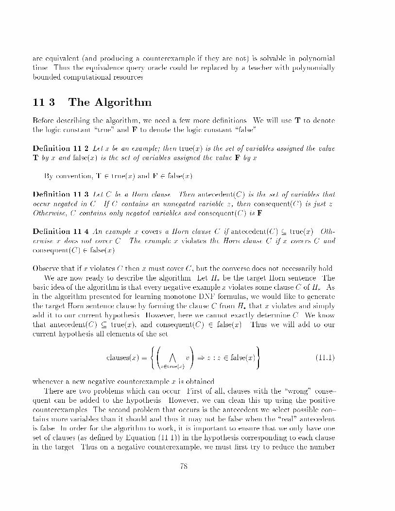
are equivalent (and producing a counterexample if they are not) is solvable in polynomial
time. Thus the equivalence query oracle could be replaced by a teacher with polynomially
bounded computational resources.
11.3 The Algorithm
Before describing the algorithm, we need a few more de�nitions. We will use T to denote
the logic constant \true" and F to denote the logic constant \false".
De�nition 11.2 Let x be an example; then true(x) is the set of variables assigned the value
T by x and false(x) is the set of variables assigned the value F by x.
By convention, T 2 true(x) and F 2 false(x).
De�nition 11.3 Let C be a Horn clause. Then antecedent(C) is the set of variables that
occur negated in C. If C contains an unnegated variable z, then consequent(C) is just z.Otherwise, C contains only negated variables and consequent(C) is F.
De�nition 11.4 An example x covers a Horn clause C if antecedent(C) � true(x). Oth-
erwise x does not cover C. The example x violates the Horn clause C if x covers C andconsequent(C) 2 false(x).
Observe that if x violates C then x must cover C, but the converse does not necessarily hold.
We are now ready to describe the algorithm. Let H� be the target Horn sentence. Thebasic idea of the algorithm is that every negative example x violates some clause C of H�. Asin the algorithm presented for learning monotone DNF formulas, we would like to generate
the target Horn sentence clause by forming the clause C from H� that x violates and simplyadd it to our current hypothesis. However, here we cannot exactly determine C. We knowthat antecedent(C) � true(x), and consequent(C) 2 false(x). Thus we will add to our
current hypothesis all elements of the set
clauses(x) =
8<:0@ ^v2true(x)
v
1A) z : z 2 false(x)
9=; (11:1)
whenever a new negative counterexample x is obtained.
There are two problems which can occur. First of all, clauses with the \wrong" conse-
quent can be added to the hypothesis. However, we can clean this up using the positive
counterexamples. The second problem that occurs is the antecedent we select possible con-tains more variables than it should and thus it may not be false when the \real" antecedent
is false. In order for the algorithm to work, it is important to ensure that we only have oneset of clauses (as de�ned by Equation (11.1)) in the hypothesis corresponding to each clause
in the target. Thus on a negative counterexample, we must �rst try to reduce the number
78
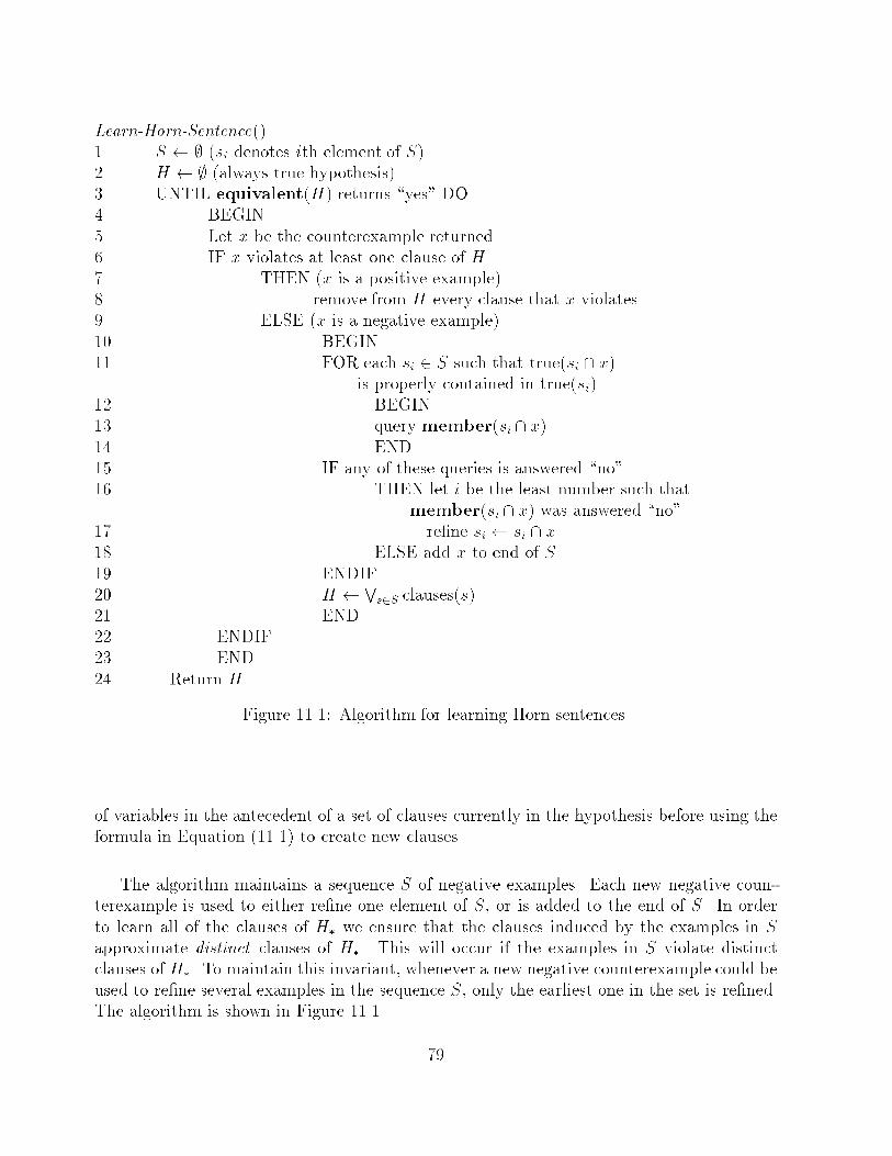
Learn-Horn-Sentence()
1 S ; (si denotes ith element of S)
2 H ; (always true hypothesis)
3 UNTIL equivalent(H) returns \yes" DO
4 BEGIN
5 Let x be the counterexample returned
6 IF x violates at least one clause of H
7 THEN (x is a positive example)
8 remove from H every clause that x violates
9 ELSE (x is a negative example)
10 BEGIN
11 FOR each si 2 S such that true(si \ x)
is properly contained in true(si)12 BEGIN13 query member(si \ x)
14 END15 IF any of these queries is answered \no"16 THEN let i be the least number such that
member(si \ x) was answered \no"17 re�ne si si \ x18 ELSE add x to end of S
19 ENDIF20 H
Ws2S clauses(s)
21 END22 ENDIF23 END
24 Return H
Figure 11.1: Algorithm for learning Horn sentences.
of variables in the antecedent of a set of clauses currently in the hypothesis before using theformula in Equation (11.1) to create new clauses.
The algorithm maintains a sequence S of negative examples. Each new negative coun-
terexample is used to either re�ne one element of S, or is added to the end of S. In order
to learn all of the clauses of H� we ensure that the clauses induced by the examples in S
approximate distinct clauses of H�. This will occur if the examples in S violate distinct
clauses of H�. To maintain this invariant, whenever a new negative counterexample could beused to re�ne several examples in the sequence S, only the earliest one in the set is re�ned.
The algorithm is shown in Figure 11.1.
79
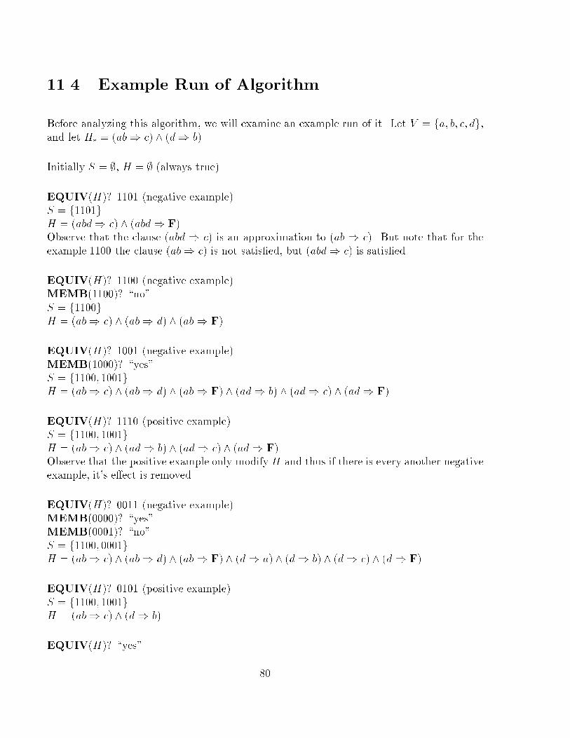
11.4 Example Run of Algorithm
Before analyzing this algorithm, we will examine an example run of it. Let V = fa; b; c; dg,and let H� = (ab) c) ^ (d) b).
Initially S = ;, H = ; (always true)
EQUIV(H)? 1101 (negative example)
S = f1101gH = (abd) c) ^ (abd) F)
Observe that the clause (abd ) c) is an approximation to (ab ) c). But note that for the
example 1100 the clause (ab) c) is not satis�ed, but (abd) c) is satis�ed.
EQUIV(H)? 1100 (negative example)MEMB(1100)? \no"
S = f1100gH = (ab) c) ^ (ab) d) ^ (ab) F)
EQUIV(H)? 1001 (negative example)
MEMB(1000)? \yes"S = f1100; 1001gH = (ab) c) ^ (ab) d) ^ (ab) F) ^ (ad) b) ^ (ad) c) ^ (ad) F)
EQUIV(H)? 1110 (positive example)S = f1100; 1001gH = (ab) c) ^ (ad) b) ^ (ad) c) ^ (ad) F)Observe that the positive example only modify H and thus if there is every another negativeexample, it's e�ect is removed.
EQUIV(H)? 0011 (negative example)
MEMB(0000)? \yes"MEMB(0001)? \no"
S = f1100; 0001gH = (ab) c) ^ (ab) d) ^ (ab) F) ^ (d) a) ^ (d) b) ^ (d) c) ^ (d) F)
EQUIV(H)? 0101 (positive example)
S = f1100; 1001gH = (ab) c) ^ (d) b)
EQUIV(H)? \yes"
80
11.5 Analysis of Algorithm
Clearly since the algorithm only halts when it receives \yes" from an equivalence query, the
hypothesis output is correct. Thus what must be shown is that the number of membership
and equivalence queries is polynomial in n and m (the number of clauses in H�), and the
computation time is polynomial in n and m. Here we shall just sketch the main ideas of the
analysis, see the Angluin, Frazier, Pitt paper [5] for the details.
The key property which must be shown is that throughout the execution of the algorithm,
at no time do two distinct elements of S violate the same clause of H�. Once this has been
shown, the remainder of the analysis is fairly straightforward. This key property is proven
using the following two lemmas.
Lemma 11.1 For each execution of the main loop of line 3, the following invariant holds.
Suppose that in step 5 of the algorithm a negative example x is obtained such that for someclause C of H� and for some si 2 S, x violates C and si covers C. Then there is some j � isuch that in step 17 the algorithm will re�ne sj by replacing it with sj \ x.
This lemma is proven by induction on the number of iterations k of the main loop of line 3.
Lemma 11.2 Let S be a sequence of elements constructed for target H� by the algorithm.Then
1. 8k8(i < k)8(C 2 H�) if sk violates C then si does not cover C
2. 8k8(i 6= k)8(C 2 H�) if sk violates C, then si does not violate C.
Here too, these two invariants are shown to hold by using an inductive proof.An immediate corollary of the second property of the second lemma is that at no time do
two distinct elements in S violate the same clause of H�. And since each of the elements inS is a negative example if follows that every element of S violates at least one clause of H�.
Thus at no time doing the execution of the algorithm does S contain more than m elements.
We are now ready to analyze the running time of the algorithm.
Theorem 11.1 A Horn sentence consisting of m clauses over n variables can be learned ex-
actly in time ~O(m3n4) using O(m2n2) equivalence queries and O(m2n) membership queries5.
Proof Sketch: The sequence S is only changed by appending a new element to it, or
re�ning an existing element. Thus jSj never decreases. Since jSj � m it follows that line18 is executed at most m times. Observe that when an element of S is re�ned in line 17, it
now contains strictly fewer variables assigned the value \true". Thus a given element can be
re�ned at most n times, and so line 17 is executed at most mn times. Whenever the ELSE
clause at line 9 is executed, either line 17 or 18 is executed. Thus lines 9{21 are executed at
5The \soft-oh" notation ~O is like the standard \big-oh" notation except that logarithmic terms areignored.
81
most nm + m = (n + 1)m times. So the total number of membership queries made are at
most (n + 1)m2.
Observe that the cardinality of clauses(s) in any hypothesis H constructed in line 15 is
at most (n+1)m. Each positive counterexample obtained in line 5 causes at least one clause
to be removed from H, thus the equivalence queries can produce at most (n+ 1)m positive
counterexamples between modi�cations of S. Therefore, line 8 is executed at most (n+1)2m2
times. Thus the total number of equivalence queries is at most (n+ 1)2m2 + (n+ 1)m + 1.
Finally, it can be shown that the time needed for each execution of the main loop is ~O(n2m).
82
CS 582T Computational Learning Theory Spring Semester, 1991
Topic 12: Learning With Abundant Irrelevant Attributes
Lecturer: Sally Goldman Scribe: Marc Wallace
12.1 Introduction
In these notes we �rst introduce the on-line (or mistake-bound) learning model. Then we
consider when this model is applied to concept classes that contain a large number of ir-
relevant attributes. Most of this lecture comes from the paper, \Learning when IrrelevantAttributes Abound: A New Linear-threshold Algorithm," by Nick Littlestone [29].
12.2 On-line Learning Model
Observe that one property of the PAC-learning model is that it is a batch model|there is aseparation between the training phase and the performance phase. Thus in the PAC modela learning session consists of two phases: the training phase and the performance phase. Inthe training phase the learner is presented with a set of instances labeled according to the
target concept c 2 Cn. At the end of this phase the learner must output a hypothesis h thatclassi�es each x 2 Xn as either a positive or negative instance. Then in the performancephase, the learner uses h to predict the classi�cation of new unlabeled instances. Since thelearner never �nds out the true classi�cation for the unlabeled instances, all learning occursin the training phase.
We now give an example from Goldman's thesis [18] to motivate the on-line learning
model . This model is also known as the mistake-bound learning model . Suppose that whenarriving at work (in Boston) you may either park in the street or park in a garage. In fact,between your o�ce building and the garage there is a street on which you can always �nd a
spot. On most days, street parking is preferable since you avoid paying the $10 garage fee.Unfortunately, when parking on the street you risk being towed ($50) due to street cleaning,
snow emergency, special events, etc. When calling the city to �nd out when they tow, youare unable to get any reasonable guidance and decide the best thing to do is just learn from
experience. There are many pieces of information that you might consider in making yourprediction; e.g. the date, the day of the week, the weather. We make the following two
assumptions: enough information is available to make good predictions if you know how
to use it, and after you commit yourself to one choice or the other you learn of the right
decision. In this example, the city has rules dictating when they tow; you just don't know
them. If you park on the street at the end of the day you know if your car was towed;otherwise when walking to the garage you see if the street is clear (i.e. you learn if you would
have been towed).
83
The on-line model is designed to study algorithms for learning to make accurate pre-
dictions in circumstances such as these. Formally, an on-line learning algorithm for C is an
algorithm that runs under the following scenario. A learning session consists of a set of trials.
In each trial, the learner is given an unlabeled instance x 2 X. The learner uses its current
hypothesis to predict if x is a positive or negative instance of the target concept c 2 C and
then the learner is told the correct classi�cation of x. If the prediction was incorrect, the
learner has made a mistake. Note that in this model there is no training phase. Instead, the
learner receives unlabeled instances throughout the entire learning session. However, after
each prediction the learner \discovers" the correct classi�cation. This feedback can then be
used by the learner to improve its hypothesis. Observe that in this model it is bene�cial
for the learning algorithm to calculate hypothesis incrementally rather than starting from
scratch each time.
In this learning model we shall evaluate the performance of a learning algorithm by thenumber of prediction mistakes made by the learning algorithm. We now describe the twomost common ways in which this notion has been formalized.
Probabilistic Mistake Bound: Let D be some arbitrary and unknown probabilitydistribution on the instance space. The probabilistic mistake bound is the probabilitythat the learner's hypothesis disagrees with c on the tth randomly drawn instance from
D. Formally, given any n � 1 and any c 2 Cn, the learner's goal is to output ahypothesis h such that the probability that h makes a mistake on the t+ 1st trial is atmost p(n)t�� for some polynomial p(n) and 0 < �.
Absolute Mistake Bound: The absolute mistake bound is the worst-case total num-
ber of mistakes made when the learner must make predictions for any, possibly in�nite,sequence of instances. (Even if the instance space is �nite, repetitions may occur.) For-mally, given any n � 1 and any c 2 Cn, the learner's goal is to make at most p(n)mistakes for some polynomial p(n).
Throughout the remainder of these notes we shall consider an on-line learning modelwhere the absolute mistake bound criterion is used. In other words, we assume that an
adversary selects the order in which the instances are presented to the learner and we evaluatethe learner by the maximum number of mistakes made during the learning session. Our goal
is to minimize the worst-case number of mistakes using an e�cient learning algorithm (i.e.each prediction is made in polynomial time). Observe that such mistake bound are quite
strong in that the order in which examples are presented does not matter; however, it is
impossible to tell how early the mistakes will occur. See Haussler et al. [21] for a discussion
of the relationship between the PAC model and on-line learning with the probabilistic mistake
bound criterion.
After studying some general results about this on-line learning model we will focus on the
situation in which the instances are drawn from the Boolean domain and proper classi�cationfor each instance can be determined by only a small fraction of the attribute space. Pattern
recognition falls under this situation since a feature detector might extract a large number
84
of features for the learner's consideration not knowing which few will prove useful. Another
example is building new concepts as Boolean functions of previously learned concepts that
are stored in a library. For this problem, the learner may need to sift through a large library
of available concepts to �nd the suitable ones to use in expressing each new concept. (The
concept class of k-DNF �ts into this model where the terms come from the library.)
12.3 De�nitions and Notation
In this section we describe the notation used by Littlestone [29]. A concept class C consists
of concepts c which are Boolean functions c : f0; 1gn ! f0; 1g.
� For any algorithm A and target concept c 2 C, let MA(c) be the maximum over all
possible sequences of examples of the number of mistakes that algorithmA makes whilelearning the concept c.
� De�ne MA(C) = maxc2CMA(c). If C is the empty set then by de�nition MA(C) = �1.
� De�ne opt(C) = minAMA(C), the minimum over all possible algorithms of the worst-case number of mistakes.
� An algorithm A is optimal for C if and only if MA(C) = opt(C).
12.4 Halving Algorithm
One algorithm which often yields a good mistake bound is the halving algorithm (as describedin Section 10.2.2). We now review the halving algorithm using the notation of Littlestone.We shall then look at a variant of it that can be shown to perform optimally.
Let consist be a subset of the concepts in C that are consistent with all previousexamples. So initially, consist = C. Given a target concept class C and an instance x, we
de�ne �i(C; x) = fc 2 Cjc(x) = ig for i = 0 or i = 1. Thus the sets �0(C; x) and �1(C; x) arethe set of concepts that are 0 at x, and the set of concepts that are 1 at x, respectively.
Upon receiving an instance x, the halving algorithm computes the sets �0(consist; x)
and �1(consist; x). If j�1(consist; x)j > j�0(consist; x)j then the algorithm predicts 1,otherwise it predicts 0. After receiving feedback the learner updates consist: if c(x) = 0
then set consist = �0(consist; x), and if c(x) = 1 then set consist = �1(consist; x).
Theorem 12.1 For any nonempty target class C, MHALV ING(C) � log2 jCj.
Proof: Since the halving algorithm predicts according to the majority, its response is con-
sistent with at least half of consist. Therefore the size of consist drops by a factor of at
least two at each mistake. And since there is a consistent function, jconsistj � 1 always,so the algorithm can make no more than log2 jCj mistakes.
The halving algorithm tells us that we can always choose a concept class such that log2 jCjmistakes are actually made. Hence we have
85
Theorem 12.2 For C such that jCj is �nite, opt(C) � log2 jCj.
Before considering an algorithm that often makes fewer mistakes than the halving algo-
rithm, we brie y consider the relation between this on-line learning model and the model
of learning with equivalence queries. If both an equivalence query algorithm and a mistake-
bound algorithm are applied to learning the same concept (over the same representation
class), we have:
# equiv. queries for exact id. � # mistakes + 1
# mistakes � # equiv. queries for exact id.
These inequalities follow from the simple observation that each mistake made in the
on-line model serves as a counterexample to an equivalence query. Furthermore, an equiva-
lence query with the correct hypothesis corresponds to a hypothesis for which no additional
mistakes will occur.
12.5 Standard Optimal Algorithm
Along with the problem that the halving algorithm often requires an exponentially amount
of time and space, it is not always an optimal algorithm. After giving some more de�nitions,we shall describe a modi�cation of the halving algorithm that always performs optimally(although is still not computationally feasible in most cases).
A mistake tree for C over X is de�ned to be a binary tree each of whose nodes is anon-empty subset of C and each of whose internal nodes is labeled with an x 2 X which
satis�es:
1. The root node is C (along with a label).
2. Given any internal node C 0 labeled with x, the left child (if present) is �0(C0; x) and
the right child (if present) is �1(C0; x).
A complete k-mistake tree is a mistake tree that is a complete binary tree of height k. (Theheight of a binary tree is the number of edges in the longest path from the root to a leaf.)
Finally, we de�ne K(C) as the largest integer k such that there exists a complete k-mistake
tree for the concept class C. We shall use the convention that K(;) = �1.In Figure 12.1 is an example of a complete 2-mistake tree. The concept class used
is a simple one; X = f0; 1g5 and C consists of the �ve concepts, fi(x1; . . . ; x5) = xi fori = 1; . . . ; 5.
As we shall show, these trees characterize the number of mistakes made by the optimal
learning algorithm.We now de�ne the standard optimal algorithm (SOA):
Let consist contain all c 2 C consistent with all past instances.
Predict 1 if K(�1(consist; x)) > K(�0(consist; x)).Predict 0 otherwise.
86
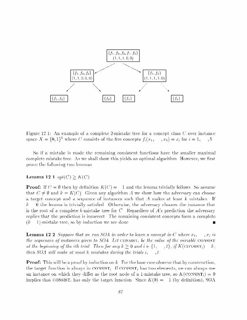
ff1; f2; f3; f4; f5g
(1; 1; 1; 0; 0)
ff1; f2; f3g
(1; 1; 0; 0; 0)
ff4; f5g
(1; 1; 1; 1; 0)
ff1; f2g ff3g ff4g ff5g
������
HHHHHj
��
@@R
��
@@R
Figure 12.1: An example of a complete 2-mistake tree for a concept class C over instancespace X = f0; 1g5 where C consists of the �ve concepts fi(x1; . . . ; x5) = xi for i = 1; . . . ; 5.
So if a mistake is made the remaining consistent functions have the smaller maximalcomplete mistake tree. As we shall show this yields an optimal algorithm. However, we �rstprove the following two lemmas.
Lemma 12.1 opt(C) � K(C).
Proof: If C = ; then by de�nition K(C) = �1 and the lemma trivially follows. So assumethat C 6= ; and k = K(C). Given any algorithm A we show how the adversary can choosea target concept and a sequence of instances such that A makes at least k mistakes. Ifk = 0 the lemma is trivially satis�ed. Otherwise, the adversary chooses the instance thatis the root of a complete k-mistake tree for C. Regardless of A's prediction the adversary
replies that the prediction is incorrect. The remaining consistent concepts form a complete(k � 1)-mistake tree, so by induction we are done.
Lemma 12.2 Suppose that we run SOA in order to learn a concept in C where x1; . . . ; xt isthe sequences of instances given to SOA. Let consisti be the value of the variable consist
at the beginning of the ith trial. Then for any k � 0 and i 2 f1; . . . ; tg, if K(consisti) = k,
then SOA will make at most k mistakes during the trials i; . . . ; t.
Proof: This will be a proof by induction on k. For the base case observe that by construction,
the target function is always in consisti. If consisti has two elements, we can always use
an instance on which they di�er as the root node of a 1-mistake tree, so K(consisti) = 0implies that consisti has only the target function. Since K(0) = �1 (by de�nition), SOA
87
cannot make any mistakes when only the target function is left. Hence the base case k = 0
is proven.
We now prove the lemma for arbitrary k > 0, assuming it holds for k � 1. If SOA makes
no mistakes during trials i; . . . ; t � 1 then the lemma is trivially true. So let j be the �rst
trial among i; . . . ; t � 1 in which a mistake is made. We now prove by contradiction that
�0(consistj,xj) and �1(consistj,xj) cannot both be complete k-mistake trees. Suppose
there are k-mistake trees for both �0(consistj,xj) and �1(consistj ,xj). Then we can com-
bine these into (k+1)-mistake tree by using xj as a root node. But by hypothesis, such a tree
cannot exist (k is the largest size of a mistake tree). Therefore one of K(�0(consistj,xj)) or
K(�1(consistj,xj)) is less than k. Since SOA always picks the larger of the two, and it made
a mistake, then K(consistj+1) will be less than k. Using induction only k� 1 mistakes will
be made from this point on. So only k mistakes can be made completing the inductive step.
Now we are ready to prove the main result of this section.
Theorem 12.3 opt(C) = MSOA(C) = K(C).
Proof: By setting i = 1 and k = K(C) in the Lemma 12.2, we get MSOA(C) � K(C).
Furthermore, by Lemma 12.1, K(C) � opt(C). Combining these two inequalities it followsthat MSOA(C) � opt(C). Finally, by de�nition, opt(C) �MSOA(C).
Let us now consider some lower bounds on opt(C). The Vapnik-Chervonenkis dimension
is useful in this respect.
Theorem 12.4 opt(C) � V CD(C).
Proof: Let fv1,. . .,vkg � X be any set shattered by C. Then clearly a complete k-mistaketree can be constructed for C, where all internal nodes at a depth i are labeled with vi+1.Apply this procedure to k = V CD(C).
We note however that this is not a tight lower bound. Let C be the a concept class of theinstance space X = f1; . . . ; 2n � 1g where C = fci : X ! f0; 1gjci(xj) = 1 if and only if j <
ig. Thus, these are concepts of \all things less than i". Clearly V CD(C) = 1 since for two
concepts ci and cj , the greater of fi; jg cannot be covered by one concept without coveringthe other. Yet, we can show that opt(C) � n by constructing a complete n-mistake tree as
follows: label the root node 2n�1. Each branch of the tree is the same type but half as big,
so by inductively constructing the binary tree, we have a complete n-mistake tree.
12.6 The Linear Threshold Algorithm: WINNOW1
In this section we describe an algorithm that e�ciently deals with a large number of irrelevant
attributes when learning in a Boolean domain. If desired this algorithm can be implementedwithin a neural network framework as a simple linear threshold function. This algorithm
is similar to the classical perceptron algorithm, except that it uses a multiplicative weight-
update scheme that permits it to perform much better than classical perceptron training
88
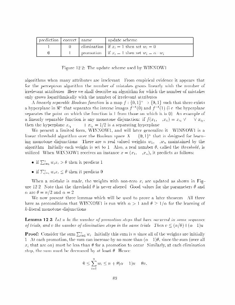
prediction correct name update scheme
1 0 elimination if xi = 1 then set wi = 0.
0 1 promotion if xi = 1 then set wi = � � wi.
Figure 12.2: The update scheme used by WINNOW1.
algorithms when many attributes are irrelevant. From empirical evidence it appears that
for the perceptron algorithm the number of mistakes grows linearly with the number of
irrelevant attributes. Here we shall describe an algorithm for which the number of mistakes
only grows logarithmically with the number of irrelevant attributes.
A linearly separable Boolean function is a map f : f0; 1gn ! f0; 1g such that there existsa hyperplane in <n that separates the inverse images f�1(0) and f�1(1) (i.e. the hyperplane
separates the point on which the function is 1 from those on which it is 0). An example ofa linearly separable function is any monotone disjunction: if f(x1,. . .,xn) = xi1 _ . . . _ xik,then the hyperplane xi1 + . . . + xik = 1=2 is a separating hyperplane.
We present a limited form, WINNOW1, and will later generalize it. WINNOW1 is a
linear threshold algorithm over the Boolean space X = f0; 1gn that is designed for learn-ing monotone disjunctions. There are n real valued weights w1,. . .,wn maintained by thealgorithm. Initially each weight is set to 1. Also, a real number �, called the threshold , isutilized. When WINNOW1 receives an instance x = (x1,. . .,xn), it predicts as follows:
� ifPn
i=1 wixi > � then it predicts 1.
� ifPn
i=1 wixi � � then it predicts 0.
When a mistake is made, the weights with non-zero xi are updated as shown in Fig-
ure 12.2. Note that the threshold � is never altered. Good values for the parameters � and� are � = n=2 and � = 2.
We now present three lemmas which will be used to prove a later theorem. All threehave as preconditions that WINNOW1 is run with � > 1 and � � 1=� for the learning of
k-literal monotone disjunctions.
Lemma 12.3 Let u be the number of promotion steps that have occurred in some sequence
of trials, and v the number of elimination steps in the same trials. Then v � (n=�)+(��1)u.
Proof: Consider the sumPn
i=1 wi. Initially this sum is n since all of the weights are initially1. At each promotion, the sum can increase by no more than (��1)�, since the sum (over all
xi that are on) must be less than � for a promotion to occur. Similarly, at each elimination
step, the sum must be decreased by at least �. Hence
0 �nXi=1
wi � n + �(�� 1)u� �v:
89
Thus
�v � n+ �(� � 1)u
giving the desired result.
Lemma 12.4 For all i, wi � �� (after any number of trials).
Proof: Since � � 1=�, for all i, initially wi � ��. We now proceed by induction on the
number of steps. Note that wi is only increased by a promotion step when xi = 1 andPni=1wixi � �. These conditions can only occur together if wi � � prior to promotion. Thus
wi � �� after the promotion step. So after any step the claim is true, hence it is always
true.
Lemma 12.5 After u promotion steps and any number of eliminations, there exists an i
such that log� wi � u=k.
Proof: Let the k-literal disjunction we are learning be of the form
f(x1; . . . ; xn) = xi1 _ . . . _ xik
Let the set R = fi1; . . . ; ikg, and consider the product P =Qj2Rwj . Since f = 0 if and only
if xj = 0 for all j 2 R, and elimination occurs when f = 0, elimination cannot a�ect theproduct P at all. Also, at each promotion step, P is increased by at least a factor of �, since
at least one of the xis was on for i 2 R. At �rst we have P = 1. After u promotions (andany number of eliminations), P � �u. Taking logs of both sides, we have
Pi2R log�wi � u.
Since jRj = k, for some i 2 R we must have that log�wi � u=k.
We are �nally ready to prove an upperbound on the number of mistakes made by WIN-NOW1 when learning a k-literal monotone disjunction.
Theorem 12.5 For the learning of k-literal monotone disjunctions, if WINNOW1 is runwith � > 1 and � � 1=�, then the total number of mistakes is at most �k(log� � + 1) + n=�.
Proof: The total number of mistakes is clearly the number of promotion steps plus thenumber of elimination steps (u+ v). Lemmas 12.4 and 12.4 yield the following bound on v:
u=k � log�wi � log� �� = log� � + 1
So
u � k(log� � + 1)
Plugging in this value of u into the inequality of Lemma 12.3, we obtain the following
bound on v:v � (n=�) + (�� 1)k(log� � + 1)
Adding the two bounds together gives the desired result.
Observe that WINNOW1 need not have prior knowledge of k although the number of
mistakes will depend on k. Littlestone's paper also discusses how to optimally choose � and� if an upperbound on k is known a priori.
Noticing that k-literal monotone disjunctions are 1-term monotone k-DNF formulas, we
state (without proof) the following lower bound on the VC dimension and thus on the numberof mistakes made in the on-line model. See Littlestone's paper for the proof.
90
Lemma 12.6 For 1 � k � n and 1 � l ��n
k
�, let C be the class of l-term monotone
k-DNF formulas. Let m be any integer with k � m � n with�m
k
�� l. Then V CD(C) �
klblog2(n=m)c.
We now apply this theorem to two special cases. If l = 1 and m = k then we get that
V CD(C) � kblog2 n=kc where C contains all conjunctions of at most k variables chosen
from n variables. Likewise, if k = 1 and m = l then V CD(C) � lblog2 nlc where C contains
all disjunctions of at most l variables chosen from n variables.
12.7 Extensions: WINNOW2
Let X = f0; 1gn be the instance space, and 0 < � � 1. We de�ne F (X; �) to be the set
of all functions X ! f0; 1g with the following property: for each f 2 F (X; �) there exist�1; . . . ; �n � 0 such that for all instances x = (x1; . . . ; xn) 2 X,
nXi=1
�ixi � 1iff(x) = 1
andnXi=1
�ixi < 1� �iff(x) = 0
That is, the inverse images of 0 and 1 are separated by at least �.An example of such a class of functions would be the r-of-k threshold functions. These
functions are de�ned by selecting k variables which are \important". Then, f(x) = 1whenever r or more of these k signi�cant variables are on. Let the selected variables bexi1; . . . ; xik.
f(x) = 1() xi1 + . . . + xik � r
Thus,f(x) = 1 () (1=r)xi1 + . . . + (1=r)xik � 1
Also,
f(x) = 0 () xi1 + . . . + xik � r � 1
Thus,f(x) = 0() (1=r)xi1 + . . . + (1=r)xik � 1 � (1=r)
Hence r-of-k threshold functions are contained in F (f0; 1gn; 1=r).We describe the algorithm WINNOW2 here. It is basically the same as WINNOW1, but
updates made in response to mistakes is slightly di�erent: instead of eliminating weights
entirely, they are divided by �. One could call this altered step a demotion. See Figure 12.3for the update scheme used by WINNOW2.
A theorem similar to the one for WINNOW1 exists to give an upper bound on the number
of mistakes that WINNOW2 will make. We state without proof the theorem here. For aproof see Littlestone's paper.
91
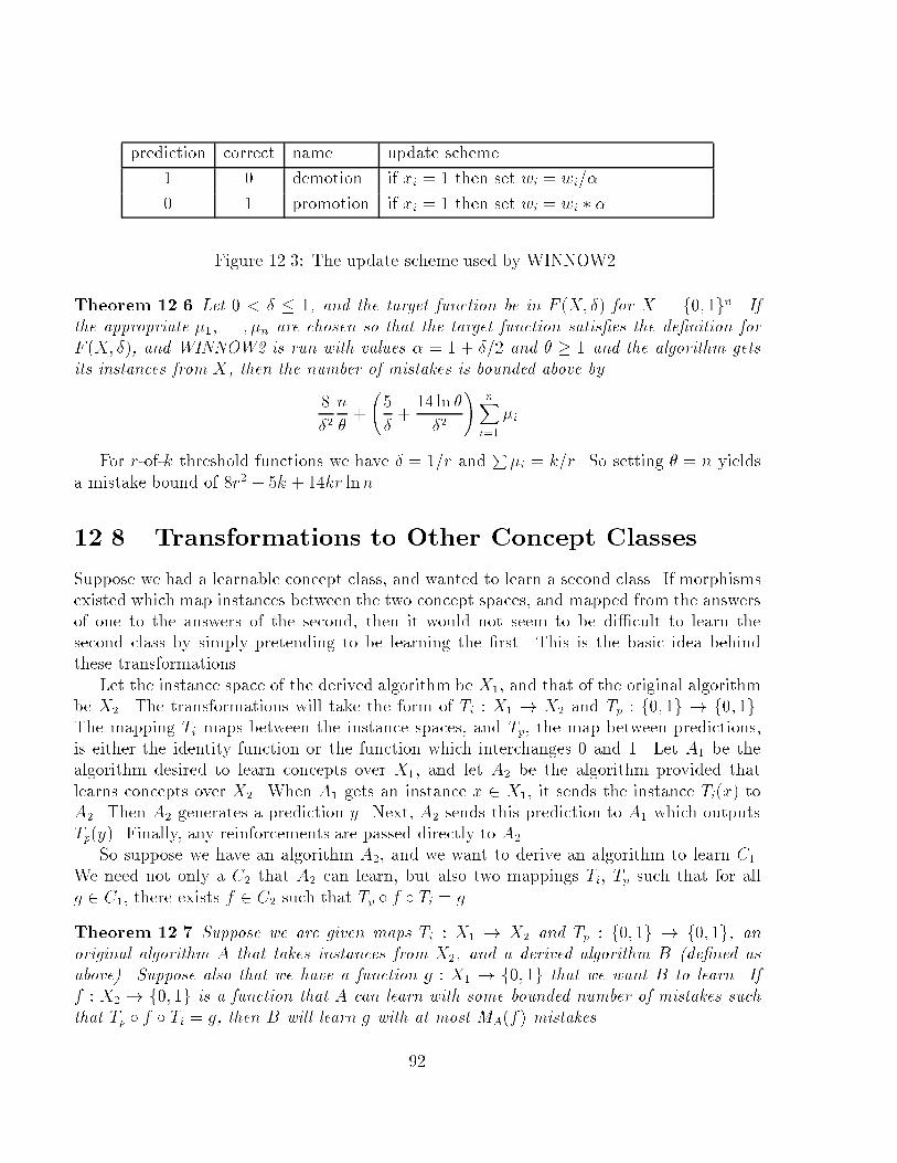
prediction correct name update scheme
1 0 demotion if xi = 1 then set wi = wi=�.
0 1 promotion if xi = 1 then set wi = wi � �.
Figure 12.3: The update scheme used by WINNOW2.
Theorem 12.6 Let 0 < � � 1, and the target function be in F (X; �) for X = f0; 1gn. If
the appropriate �1; . . . ; �n are chosen so that the target function satis�es the de�nition for
F (X; �), and WINNOW2 is run with values � = 1 + �=2 and � � 1 and the algorithm gets
its instances from X, then the number of mistakes is bounded above by
8
�2n
�+
5
�+
14 ln �
�2
!nXi=1
�i
For r-of-k threshold functions we have � = 1=r andP�i = k=r. So setting � = n yields
a mistake bound of 8r2 + 5k + 14kr lnn.
12.8 Transformations to Other Concept Classes
Suppose we had a learnable concept class, and wanted to learn a second class. If morphismsexisted which map instances between the two concept spaces, and mapped from the answersof one to the answers of the second, then it would not seem to be di�cult to learn thesecond class by simply pretending to be learning the �rst. This is the basic idea behindthese transformations.
Let the instance space of the derived algorithm be X1, and that of the original algorithmbe X2. The transformations will take the form of Ti : X1 ! X2 and Tp : f0; 1g ! f0; 1g.The mapping Ti maps between the instance spaces, and Tp, the map between predictions,
is either the identity function or the function which interchanges 0 and 1. Let A1 be thealgorithm desired to learn concepts over X1, and let A2 be the algorithm provided that
learns concepts over X2. When A1 gets an instance x 2 X1, it sends the instance Ti(x) toA2. Then A2 generates a prediction y. Next, A2 sends this prediction to A1 which outputs
Tp(y). Finally, any reinforcements are passed directly to A2.So suppose we have an algorithm A2, and we want to derive an algorithm to learn C1.
We need not only a C2 that A2 can learn, but also two mappings Ti, Tp such that for all
g 2 C1, there exists f 2 C2 such that Tp � f � Ti = g.
Theorem 12.7 Suppose we are given maps Ti : X1 ! X2 and Tp : f0; 1g ! f0; 1g, anoriginal algorithm A that takes instances from X2, and a derived algorithm B (de�ned as
above). Suppose also that we have a function g : X1 ! f0; 1g that we want B to learn. Iff : X2 ! f0; 1g is a function that A can learn with some bounded number of mistakes such
that Tp � f � Ti = g, then B will learn g with at most MA(f) mistakes.
92
Proof: This proof is trivial. Basically, B can only make a mistake when A has.
We now go through several example transformations.
Example 12.1 Arbitrary Disjunctions
We �rst consider learning arbitrary disjunctions, using WINNOW1 as A1. We can deter-
mine the correct signs (negated variable or not) for all variables by �nding a single negative
example. Predict positive until we get a negative example (one mistake at most). Let
(z1; . . . ; zn) be the negative example. All future instances are sent to WINNOW1 using
Ti(x1; . . . ; xn) = (x1 � z1; . . . ; xn � zn):
Such a mapping makes sense, since if zi is o� in the negative example, it cannot be anegated variable, and vice versa, so only the negated variables are negated by the mapping.(What is done to irrelevant variables does not matter.) Finally, let Tp be the identityfunction. It is easily shown that the conditions of Theorem 12.7 are satis�ed. So the mistakebound for learning non-monotone disjunctions with this technique is just one more than the
corresponding mistake bound for learning monotone disjunctions.
Example 12.2 Arbitrary Conjunctions
The example of arbitrary disjunctions can be extended to learning k-literal monotoneconjunctions. Let A2 be the algorithm described in the above example, let Ti = (1 �x1; . . . ; 1 � xn), and let Tp(r) = 1 � r. Again, using DeMorgan's law it is easily veri�edthat the conditions of Theorem 12.7 hold. Thus, the number of mistakes will be bounded
by 2k log2 n + 2.
Example 12.3 k-DNF for �xed k
As another example, consider learning k-DNF for a �xed k. We notice that this class is moredi�cult, since it is not a linearly separable class. Let the original algorithm be WINNOW1over k-literal disjunctions. Let n1 be the number of variables in the derived concept class,
and let n2, the number of variables over which the original algorithm is run, be set to
n2 =Pk
i=0 2i�n
i
�. Then we have that
Ti(x) = (c1(x); . . . ; cn2(x))
where x = (x1; . . . ; xn1) and the ci's range over all possible conjunctions which could beterms in a k-DNF formula. Notice that given any k-DNF we can represent it as such. If
such a g is given we can construct an f in the derived space which is a disjunction of all thevariables whose corresponding terms are in the expansion of g.
By expanding the summation for n2, we can see that n2 � (2n)k + 1. Since the original
algorithm will be learning an l-literal monotone disjunction, we will make O(l log nk) =
93
O(lk log n) mistakes. Compare this to the algorithm Valiant presented which can be forced
to make�n
k
�� l mistakes in the worst case.
By using the VC dimension, we can �nd a lower bound on the mistake bound. Taking
m = dkl1=ke, we have m
k
!�mk
kk� 1
Thus a lower bound would be given, when kl1=k � n, by:
kl
$log2
n
dkl1=ke
%
If, however, l is known, an even better bound of 4l + 2kl log2
�2nl1=k
�can be achieved.
94
CS 582T Computational Learning Theory Spring Semester, 1991
Topic 13: Learning Regular Sets
Lecturer: Sally Goldman Scribe: Ellen Witte
13.1 Introduction
In this lecture we consider the problem of learning an unknown regular set using member-
ship and equivalence queries. The material presented in this lecture comes from the paper,
\Learning Regular Sets from Queries and Counterexamples," by Dana Angluin [2]. Sincedeterministic �nite-state acceptors (dfa's) recognize the same languages as regular sets, thisis equivalent to the problem of learning an unknown dfa. We will express our hypothesis
in the form of a dfa by giving the initial state, �nal (accepting) states and transition func-tion. Our goal will be to �nd a dfa with the minimum number of states that recognizes theunknown regular set.
Gold [15] has shown that �nding a minimum dfa consistent with an arbitrary set ofpositive and negative examples is NP-hard. The learning algorithm has the advantage ofbeing able to select the examples for the membership queries, thus the set of examples usedto help construct the dfa is not arbitrary. To be certain we are not asking for too much with
membership and equivalence queries, we would like both types of queries to be computablein time polynomial in the number of states in a minimum dfa recognizing the regular setand polynomial in the length of the hypothesis dfa. The teacher has access to the minimumdfa, thus a membership query can be answered by simply tracing the dfa using the givenstring. In addition, there is a polynomial time algorithm for testing the equivalence of twodfa's which returns a counterexample if the dfa's are not equivalent.
13.2 The Learning Algorithm
In the following discussion we use the notation L� to denote the learning algorithm, U todenote the unknown regular set to be learned, and A to denote the alphabet of the regularlanguage. (The alphabet is known to the learner.)
The learning algorithm develops a hypothesis by using membership queries to determinewhether or not certain strings are in the set U . The results of these queries are stored in
an observation table maintained by the learner. Periodically the learner will construct a
hypothesis dfa from the observation table and perform an equivalence query to see if thehypothesis is correct. If the hypothesis is not correct then the counterexample will be used
to modify the observation table. Next we describe the structure of the observation table.Later we will see how the hypothesis dfa is constructed from the table.
95
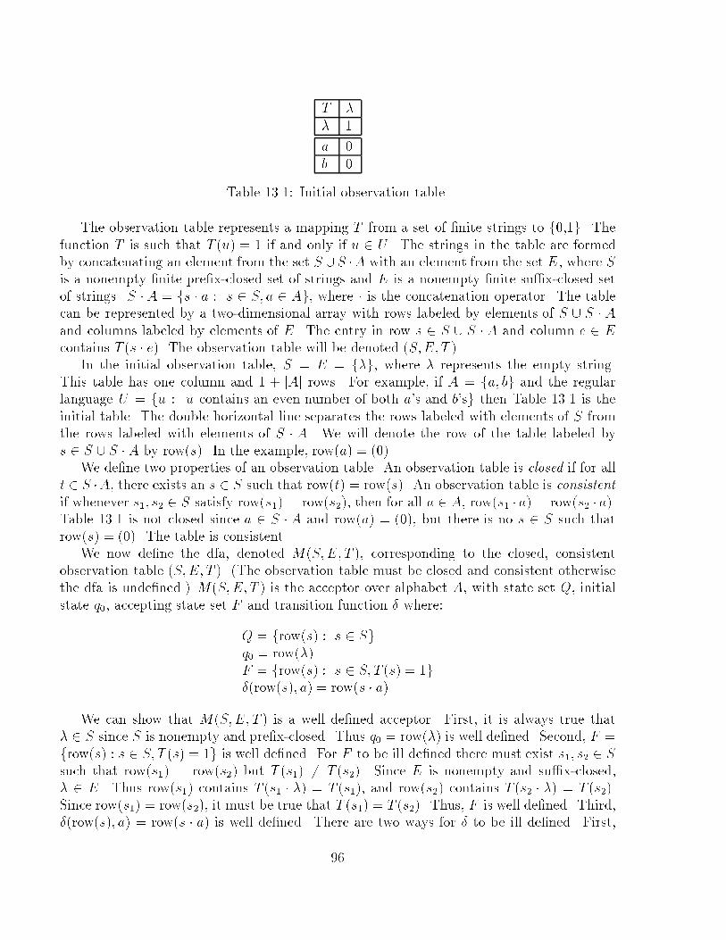
T �
� 1
a 0
b 0
Table 13.1: Initial observation table.
The observation table represents a mapping T from a set of �nite strings to f0,1g. The
function T is such that T (u) = 1 if and only if u 2 U . The strings in the table are formed
by concatenating an element from the set S [S �A with an element from the set E, where S
is a nonempty �nite pre�x-closed set of strings and E is a nonempty �nite su�x-closed set
of strings. S �A = fs � a : s 2 S; a 2 Ag, where � is the concatenation operator. The table
can be represented by a two-dimensional array with rows labeled by elements of S [ S � Aand columns labeled by elements of E. The entry in row s 2 S [ S � A and column e 2 Econtains T (s � e). The observation table will be denoted (S;E; T ).
In the initial observation table, S = E = f�g, where � represents the empty string.This table has one column and 1 + jAj rows. For example, if A = fa; bg and the regularlanguage U = fu : u contains an even number of both a's and b'sg then Table 13.1 is the
initial table. The double horizontal line separates the rows labeled with elements of S fromthe rows labeled with elements of S � A. We will denote the row of the table labeled bys 2 S [ S �A by row(s). In the example, row(a) = (0).
We de�ne two properties of an observation table. An observation table is closed if for allt 2 S �A, there exists an s 2 S such that row(t) = row(s). An observation table is consistent
if whenever s1; s2 2 S satisfy row(s1) = row(s2), then for all a 2 A, row(s1 � a) = row(s2 � a).Table 13.1 is not closed since a 2 S � A and row(a) = (0), but there is no s 2 S such thatrow(s) = (0). The table is consistent.
We now de�ne the dfa, denoted M(S;E; T ), corresponding to the closed, consistentobservation table (S;E; T ). (The observation table must be closed and consistent otherwisethe dfa is unde�ned.) M(S;E; T ) is the acceptor over alphabet A, with state set Q, initial
state q0, accepting state set F and transition function � where:
Q = frow(s) : s 2 Sgq0 = row(�)
F = frow(s) : s 2 S; T (s) = 1g�(row(s); a) = row(s � a)
We can show that M(S;E; T ) is a well de�ned acceptor. First, it is always true that� 2 S since S is nonempty and pre�x-closed. Thus q0 = row(�) is well de�ned. Second, F =
frow(s) : s 2 S; T (s) = 1g is well de�ned. For F to be ill de�ned there must exist s1; s2 2 Ssuch that row(s1) = row(s2) but T (s1) 6= T (s2). Since E is nonempty and su�x-closed,� 2 E. Thus row(s1) contains T (s1 � �) = T (s1), and row(s2) contains T (s2 � �) = T (s2).
Since row(s1) = row(s2), it must be true that T (s1) = T (s2). Thus, F is well de�ned. Third,
�(row(s); a) = row(s � a) is well de�ned. There are two ways for � to be ill de�ned. First,
96
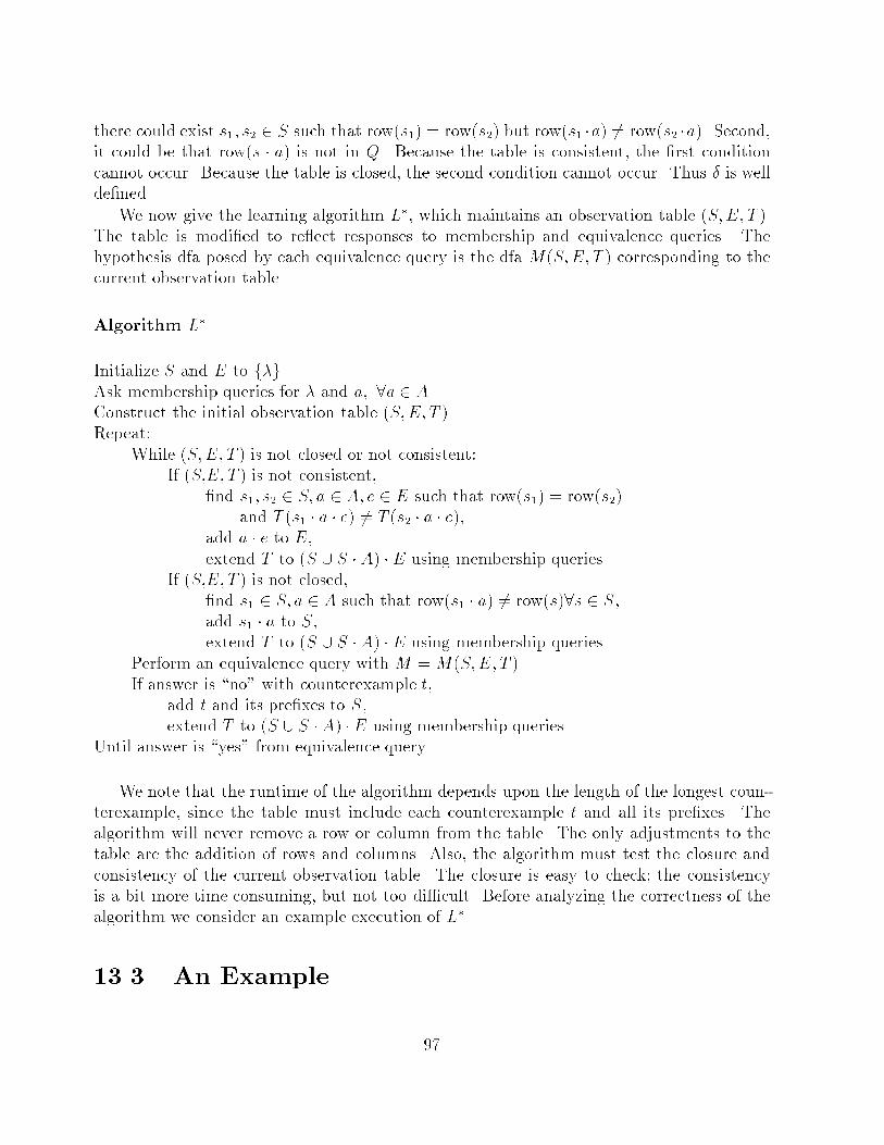
there could exist s1; s2 2 S such that row(s1) = row(s2) but row(s1 �a) 6= row(s2 �a). Second,
it could be that row(s � a) is not in Q. Because the table is consistent, the �rst condition
cannot occur. Because the table is closed, the second condition cannot occur. Thus � is well
de�ned.
We now give the learning algorithm L�, which maintains an observation table (S;E; T ).
The table is modi�ed to re ect responses to membership and equivalence queries. The
hypothesis dfa posed by each equivalence query is the dfa M(S;E; T ) corresponding to the
current observation table.
Algorithm L�
Initialize S and E to f�g.Ask membership queries for � and a; 8a 2 A.Construct the initial observation table (S;E; T ).Repeat:
While (S;E; T ) is not closed or not consistent:If (S;E; T ) is not consistent,
�nd s1; s2 2 S; a 2 A; e 2 E such that row(s1) = row(s2)and T (s1 � a � e) 6= T (s2 � a � e),
add a � e to E,
extend T to (S [ S �A) � E using membership queries.If (S;E; T ) is not closed,
�nd s1 2 S; a 2 A such that row(s1 � a) 6= row(s)8s 2 S,add s1 � a to S,extend T to (S [ S �A) � E using membership queries.
Perform an equivalence query with M = M(S;E; T ).If answer is \no" with counterexample t,
add t and its pre�xes to S,extend T to (S [ S �A) � E using membership queries.
Until answer is \yes" from equivalence query.
We note that the runtime of the algorithm depends upon the length of the longest coun-
terexample, since the table must include each counterexample t and all its pre�xes. The
algorithm will never remove a row or column from the table. The only adjustments to thetable are the addition of rows and columns. Also, the algorithm must test the closure and
consistency of the current observation table. The closure is easy to check; the consistencyis a bit more time consuming, but not too di�cult. Before analyzing the correctness of the
algorithm we consider an example execution of L�.
13.3 An Example
97
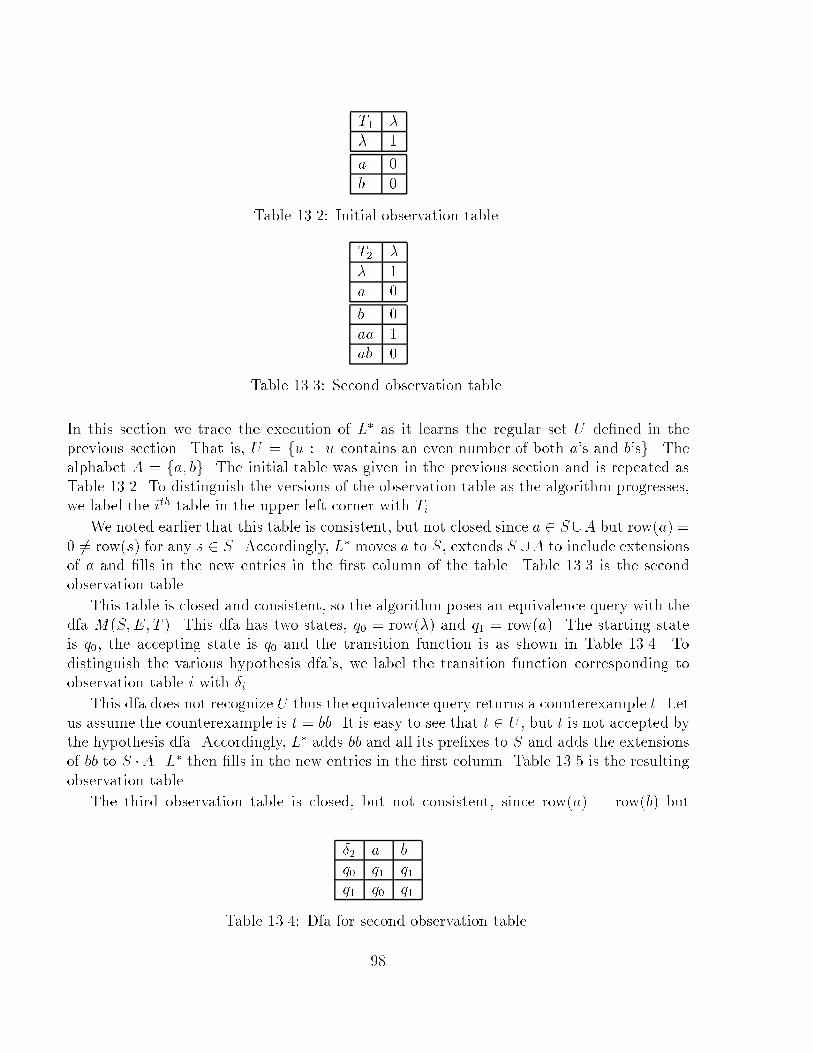
T1 �
� 1
a 0
b 0
Table 13.2: Initial observation table.
T2 �
� 1
a 0
b 0
aa 1
ab 0
Table 13.3: Second observation table.
In this section we trace the execution of L� as it learns the regular set U de�ned in theprevious section. That is, U = fu : u contains an even number of both a's and b'sg. Thealphabet A = fa; bg. The initial table was given in the previous section and is repeated asTable 13.2. To distinguish the versions of the observation table as the algorithm progresses,we label the ith table in the upper left corner with Ti.
We noted earlier that this table is consistent, but not closed since a 2 S[A but row(a) =
0 6= row(s) for any s 2 S. Accordingly, L� moves a to S, extends S [A to include extensionsof a and �lls in the new entries in the �rst column of the table. Table 13.3 is the secondobservation table.
This table is closed and consistent, so the algorithm poses an equivalence query with thedfa M(S;E; T ). This dfa has two states, q0 = row(�) and q1 = row(a). The starting stateis q0, the accepting state is q0 and the transition function is as shown in Table 13.4. To
distinguish the various hypothesis dfa's, we label the transition function corresponding toobservation table i with �i.
This dfa does not recognize U thus the equivalence query returns a counterexample t. Letus assume the counterexample is t = bb. It is easy to see that t 2 U , but t is not accepted by
the hypothesis dfa. Accordingly, L� adds bb and all its pre�xes to S and adds the extensions
of bb to S �A. L� then �lls in the new entries in the �rst column. Table 13.5 is the resulting
observation table.
The third observation table is closed, but not consistent, since row(a) = row(b) but
�2 a b
q0 q1 q1q1 q0 q1
Table 13.4: Dfa for second observation table.
98
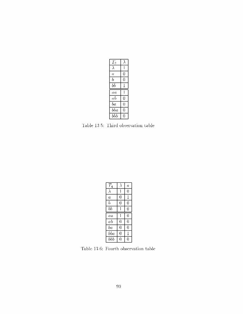
T3 �
� 1
a 0
b 0
bb 1
aa 1
ab 0
ba 0
bba 0
bbb 0
Table 13.5: Third observation table.
T4 � a
� 1 0
a 0 1
b 0 0
bb 1 0
aa 1 0
ab 0 0
ba 0 0
bba 0 1
bbb 0 0
Table 13.6: Fourth observation table.
99
�4 a b
q0 q1 q2q1 q0 q2q2 q2 q0
Table 13.7: Dfa for fourth observation table.
T5 � a
� 1 0
a 0 1
b 0 0
bb 1 0
ab 0 0
abb 0 1
aa 1 0
ba 0 0
bba 0 1
bbb 0 0
aba 0 0
abba 1 0
abbb 0 0
Table 13.8: Fifth observation table.
row(aa) 6= row(ba). The algorithm adds a to E and �lls in the values of T for the new
column. Table 13.6 is the result.
Table 13.6 is a closed, consistent observation table. The algorithm constructs the dfaM(S;E; T ), which has three states, q0 = row(�), q1 = row(a) and q2 = row(b). The startingstate is q0, the accepting state is q0 and the transition function is as shown in Table 13.7.
This dfa is not quite correct, thus the equivalence query returns a counterexample t. Let
us assume the counterexample is t = abb, which is not in U but is accepted by the dfa. Thealgorithm adds abb and all its pre�xes and extensions to the observation table and �lls in
the values of T . Table 13.8 shows the result.
Table 13.8 is closed, but not consistent since row(b) = row(ab) but row(bb) 6= row(abb).
The algorithm adds b to E and �lls in the values of T for this new column. The result is
Table 13.9.
This table is closed and consistent, so the algorithm constructs M(S;E; T ). This dfa hasfour states, q0 = row(�), q1 = row(a), q2 = row(b) and q3 = row(ab). The starting state is
q0, the accepting state is q0 and the transition function is as shown in Table 13.10.
This dfa accepts exactly the language U , thus the equivalence query returns \yes" andthe algorithm halts. This is the minimum size dfa to recognize the language consisting of all
strings with an even number of a's and an even number of b's.
100
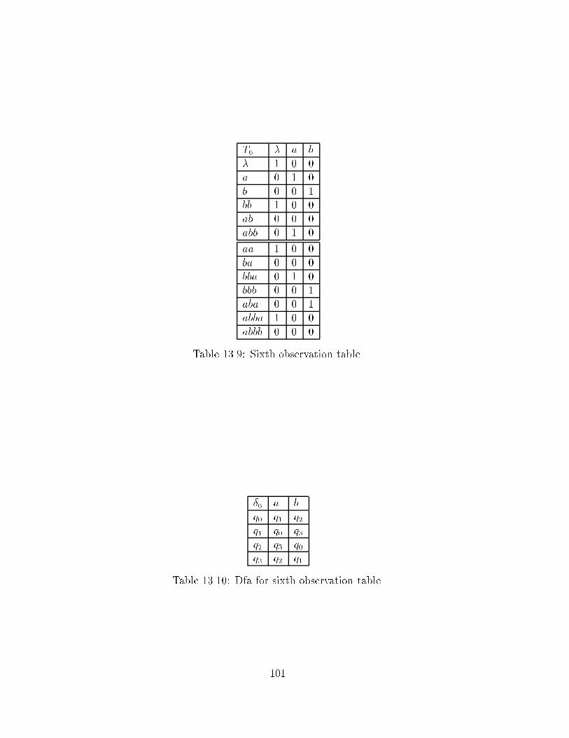
T6 � a b
� 1 0 0
a 0 1 0
b 0 0 1
bb 1 0 0
ab 0 0 0
abb 0 1 0
aa 1 0 0
ba 0 0 0
bba 0 1 0
bbb 0 0 1
aba 0 0 1
abba 1 0 0
abbb 0 0 0
Table 13.9: Sixth observation table.
�6 a b
q0 q1 q2q1 q0 q3q2 q3 q0q3 q2 q1
Table 13.10: Dfa for sixth observation table.
101
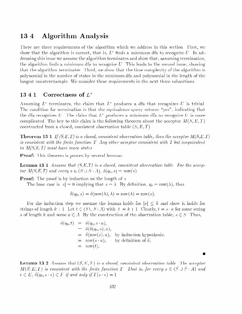
13.4 Algorithm Analysis
There are three requirements of the algorithm which we address in this section. First, we
show that the algorithm is correct, that is, L� �nds a minimum dfa to recognize U . In ad-
dressing this issue we assume the algorithm terminates and show that, assuming termination,
the algorithm �nds a minimum dfa to recognize U . This leads to the second issue, showing
that the algorithm terminates. Third, we show that the time complexity of the algorithm is
polynomial in the number of states in the minimum dfa and polynomial in the length of the
longest counterexample. We consider these requirements in the next three subsections.
13.4.1 Correctness of L�
Assuming L� terminates, the claim that L� produces a dfa that recognizes U is trivial.The condition for termination is that the equivalence query returns \yes", indicating thatthe dfa recognizes U . The claim that L� produces a minimum dfa to recognize U is more
complicated. The key to this claim is the following theorem about the acceptor M(S;E; T )constructed from a closed, consistent observation table (S;E; T ).
Theorem 13.1 If (S,E,T) is a closed, consistent observation table, then the acceptor M(S,E,T)is consistent with the �nite function T. Any other acceptor consistent with T but inequivalentto M(S,E,T) must have more states.
Proof: This theorem is proven by several lemmas.
Lemma 13.1 Assume that (S,E,T) is a closed, consistent observation table. For the accep-tor M(S,E,T) and every s 2 (S [ S �A), �(q0; s) = row(s).
Proof: The proof is by induction on the length of s.The base case is jsj = 0 implying that s = �. By de�nition, q0 = row(�), thus
�(q0; s) = �(row(�); �) = row(�) = row(s):
For the induction step we assume the lemma holds for jsj � k and show it holds forstrings of length k + 1. Let t 2 (S [ S �A) with jtj = k+ 1. Clearly, t = s � a for some strings of length k and some a 2 A. By the construction of the observation table, s 2 S. Thus,
�(q0; t) = �(q0; s � a);
= �(�(q0; s); a);
= �(row(s); a); by induction hypothesis;= row(s � a); by de�nition of �;
= row(t):
Lemma 13.2 Assume that (S;E; T ) is a closed, consistent observation table. The acceptor
M(S;E; T ) is consistent with the �nite function T . That is, for every s 2 (S [ S � A) ande 2 E, �(q0; s � e) 2 F if and only if T (s � e) = 1.
102
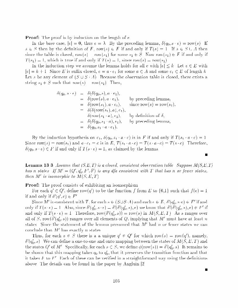
Proof: The proof is by induction on the length of e.
In the base case, jej = 0, thus e = �. By the preceding lemma, �(q0; s � e) = row(s). If
s 2 S then by the de�nition of F , row(s) 2 F if and only if T (s) = 1. If s 2 S [ A then
since the table is closed, row(s) = row(s1) for some s1 2 S. Now row(s1) 2 F if and only if
T (s1) = 1, which is true if and only if T (s) = 1, since row(s) = row(s1).
In the induction step we assume the lemma holds for all e with jej � k. Let e 2 E with
jej = k + 1. Since E is su�x closed, e = a � e1 for some a 2 A and some e1 2 E of length k.
Let s be any element of (S [ S � A). Because the observation table is closed, there exists a
string s1 2 S such that row(s) = row(s1). Then,
�(q0; s � e) = �(�(q0; s); a � e1);= �(row(s); a � e1); by preceding lemma;
= �(row(s1); a � e1); since row(s) = row(s1);
= �(�(row(s1); a); e1);= �(row(s1 � a); e1); by de�nition of �;= �(�(q0; s1 � a); e1); by preceding lemma;= �(q0; s1 � a � e1):
By the induction hypothesis on e1, �(q0; s1 � a � e) is in F if and only if T (s1 � a � e) = 1.Since row(s) = row(s1) and a � e1 = e is in E, T (s1 � a � e) = T (s � a � e) = T (s � e). Therefore,
�(q0; s � e) 2 F if and only if T (s � e) = 1, as claimed by the lemma.
Lemma 13.3 Assume that (S,E,T) is a closed, consistent observation table. Suppose M(S,E,T)has n states. If M 0 = (Q0; q00; F
0; �0) is any dfa consistent with T that has n or fewer states,then M 0 is isomorphic to M(S;E; T ).
Proof: The proof consists of exhibiting an isomorphism.For each q0 2 Q0, de�ne row(q0) to be the function f from E to f0,1g such that f(e) = 1
if and only if �0(q0; e) 2 F 0.
SinceM 0 is consistent with T , for each s 2 (S[S�A) and each e 2 E, �0(q00; s�e) 2 F0 if and
only if T (s � e) = 1. Also, since �0(q00; s � e) = �0(�0(q00; s); e) we know that �0(�0(q00; s); e) 2 F0 if
and only if T (s � e) = 1. Therefore, row(�0(q00; s)) = row(s) in M(S;E; T ). As s ranges over
all of S, row(�0(q00; s)) ranges over all elements of Q, implying that M 0 must have at least n
states. Since the statement of the lemma presumed that M 0 had n or fewer states we can
conclude that M 0 has exactly n states.Thus, for each s 2 S there is a a unique q0 2 Q0 for which row(s) = row(q0), namely,
�0(q00; s). We can de�ne a one-to-one and onto mapping between the states of M(S;E; T ) and
the states Q0 of M 0. Speci�cally, for each s 2 S, we de�ne �(row(s)) = �0(q00; s). It remains to
be shown that this mapping takes q0 to q00, that it preserves the transition function and thatit takes F to F 0. Each of these can be veri�ed in a straightforward way using the de�nitions
above. The details can be found in the paper by Angluin [2].
103

Lemma 2 and Lemma 3 together prove the two parts of Theorem 1. Namely, Lemma
2 shows that M(S;E; T ) is consistent with T and Lemma 3 shows that any dfa consistent
with T is either isomorphic to M(S;E; T ) or has more states. Thus M(S;E; T ) is a smallest
dfa consistent with T .
13.4.2 Termination of L�
In the previous subsection we ignored the question of whether or not L� will terminate and
concentrated on showing that if it terminates, the output will be correct. In this subsection
we address the issue of termination.
To see that the algorithm will terminate we need the following lemma. At �rst glance the
lemma appears similar to the last lemma of the previous section. The key di�erence is that
the following lemma does not assume that the observation table is closed and consistent. Itis important to consider this more general case because as the algorithm proceeds, there willbe times when the observation table is not closed and consistent.
Lemma 13.4 Let (S;E; T ) be an observation table. Let n denote the number of di�erent
values of row(s) for s 2 S. (Note that if (S;E; T ) is closed and consistent, then this will bethe number of states in M(S;E; T ).) Any dfa consistent with T must have at least n states.
Proof:
Let M = (Q; �; q0; F ) be a dfa consistent with T . De�ne f(s) = �(q0; s) for everys 2 S. In other words, f(s) is the �nal state of M when run with input s. Suppose s1and s2 are elements of S such that row(s1) 6= row(s2). Then there exists an e 2 E such
that T (s1 � e) 6= T (s2 � e). Since M is consistent with T , exactly one of �(q0; s1 � e) and�(q0; s2 � e) is in F . Thus, �(q0; s1 � e) and �(q0; s2 � e) must be distinct states, implying thatf(s1 � e) 6= f(s2 � e). Since there are n di�erent values of row(s), f(s) must take on at leastn distinct values. Thus M has at least n states.
Let n be the number of states in a minimum dfa MU for the unknown language U . Toprove termination we show that the number of distinct values of row(s) for s 2 S increases
monotonically up to n as L� runs.First, consider what happens when a string is added to E because the table is not
consistent. The number of distinct values of row(s) must increase by at least one. Two
previously equal values, row(s1) and row(s2), are no longer equal after E is augmented. Any
two unequal values will remain unequal.Second, consider what happens when a string s1 � a is added to S because the table is
not closed. By de�nition, row(s1 � a) di�ers from row(s) for all s 2 S. Thus the number ofdistinct values of row(s) is increased by at least one.
From these two situations we can conclude that the total number of operations of either
type over the entire run of L� is at most n � 1. (There is initially one value of row(s) andthere cannot be more than n.) Thus the algorithm will enter the while loop at most n � 1
times. This means that L� always eventually �nds a closed, consistent observation table(S;E; T ) and makes an equivalence query with M(S;E; T ).
104
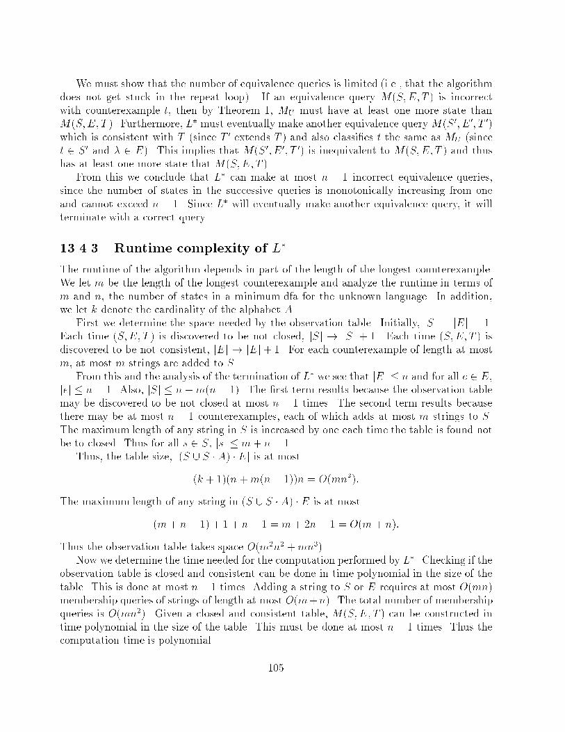
We must show that the number of equivalence queries is limited (i.e., that the algorithm
does not get stuck in the repeat loop). If an equivalence query M(S;E; T ) is incorrect
with counterexample t, then by Theorem 1, MU must have at least one more state than
M(S;E; T ). Furthermore, L� must eventually make another equivalence query M(S0; E 0; T 0)
which is consistent with T (since T 0 extends T ) and also classi�es t the same as MU (since
t 2 S0 and � 2 E). This implies that M(S0; E0; T 0) is inequivalent to M(S;E; T ) and thus
has at least one more state that M(S;E; T ).
From this we conclude that L� can make at most n � 1 incorrect equivalence queries,
since the number of states in the successive queries is monotonically increasing from one
and cannot exceed n � 1. Since L� will eventually make another equivalence query, it will
terminate with a correct query.
13.4.3 Runtime complexity of L�
The runtime of the algorithm depends in part of the length of the longest counterexample.We let m be the length of the longest counterexample and analyze the runtime in terms of
m and n, the number of states in a minimum dfa for the unknown language. In addition,we let k denote the cardinality of the alphabet A.
First we determine the space needed by the observation table. Initially, jSj = jEj = 1.Each time (S;E; T ) is discovered to be not closed, jSj ! jSj + 1. Each time (S;E; T ) isdiscovered to be not consistent, jEj ! jEj+ 1. For each counterexample of length at most
m, at most m strings are added to S.From this and the analysis of the termination of L� we see that jEj � n and for all e 2 E,
jej � n � 1. Also, jSj � n+ m(n� 1). The �rst term results because the observation tablemay be discovered to be not closed at most n � 1 times. The second term results becausethere may be at most n � 1 counterexamples, each of which adds at most m strings to S.
The maximum length of any string in S is increased by one each time the table is found notbe to closed. Thus for all s 2 S, jsj � m+ n� 1.
Thus, the table size, j(S [ S �A) � Ej is at most
(k + 1)(n +m(n� 1))n = O(mn2):
The maximum length of any string in (S [ S �A) � E is at most
(m+ n � 1) + 1 + n� 1 = m+ 2n � 1 = O(m + n):
Thus the observation table takes space O(m2n2 +mn3).
Now we determine the time needed for the computation performed by L�. Checking if the
observation table is closed and consistent can be done in time polynomial in the size of the
table. This is done at most n� 1 times. Adding a string to S or E requires at most O(mn)
membership queries of strings of length at most O(m+n). The total number of membershipqueries is O(mn2). Given a closed and consistent table, M(S;E; T ) can be constructed in
time polynomial in the size of the table. This must be done at most n� 1 times. Thus the
computation time is polynomial.
105
Finally, note that if the counterexamples are always of the minimum possible length then
m � n and all results are polynomial in n. The algorithm which tests for the equivalence of
two dfa's can identify a counterexample of minimum length. Also, the bound on the number
of membership queries was improved to O(kn2 + n logm) by Rivest and Schapire [36].
106
CS 582T Computational Learning Theory Spring Semester, 1991
Topic 14: Results on Learnability and the VC Dimension
Lecturer: Sally Goldman Scribe: Weilan Wu
14.1 Introduction
In these notes we more carefully study the relationship between the Vapnik-Chervonenkis Di-
mension and the sample complexity of PAC learning. The material presented here comes from
the paper \Results on Learnability and the Vapnik-Chervonenkis Dimension," by Nathan
Linial, Yishay Mansour, and Ronald Rivest [28].Recall in Topic 7 that we studied a result of Blumer, et al. [12] stating that a concept class
C which is non-trivial and well-behaved is PAC learnable if and only if the VC dimensionof C is �nite. Here we demonstrate that by using dynamic sampling versus static sampling
that one can PAC learn some concept classes with in�nite VC dimension. In other words,the Blumer, Ehrenfeucht, Haussler and Warmuth result assumes that the learner asks for asingle sample of a given size and must then processes these examples. If instead the learnercan divide the learning session into stages where in each stage the learner asks for someexamples and then performs some processing, then it is possible to learn any concept class
that can be written as the countable union
C = C1 [ C2 [ � � �
where each concept class Cd has VC-dimension at most d.
In these notes we shall say that a concept class C is PAC learnable if there exists a learningalgorithm that outputs a hypothesis meeting the PAC criterion. We say a concept class Cis polynomially PAC learnable if it uses time and sample complexity that are polynomial in1�
and 1�.
All previous PAC algorithms that we have studied assume a static sampling model in
which the learning algorithm must draw all examples before any computation is performed.In addition to using a static sampling model, typically PAC learning algorithms are consistent
in that the concept C they return agrees with the classi�cation of each example of the sample.
Using this notation, we will restate the (Blumer et al. [12]) result as below.
Theorem 14.1 A concept class C is PAC learnable with static sampling if and only if Chas �nite V C-dimension. Furthermore the bounds of the sample complexity are:
m(�; �) = O
1
�ln
1
�+d
�ln
1
�
!
and
m(�; �) =
1
�ln
1
�+d
�
!
107
Based on these bounds, Blumer et. al. also showed many concept classes to be polyno-
mially PAC learnable. More generally, if C is a class with �nite VC dimension and there
exists a polynomial time algorithm to �nd a concept in C that is consistent with a given
sample, then C is polynomially PAC learnable.
14.2 Dynamic Sampling
Now we consider the notion of dynamic sampling, in which the number of examples examined
increases with the complexity of target concept. It turns out that dynamic sampling does
indeed enrich the class of PAC learnable concepts, compared to static sampling. By this
method, one can establish the learnability of various concept class with an in�nite Vapnik-
Chervonenkis dimension.
When using dynamic sampling, the PAC learning algorithm alternates between drawingexamples and doing computations. A stage of the PAC learning algorithm of consists ofdrawing a set examples and performing the subsequent computations. Thus a static sampling
algorithm is equivalent to a one-stage dynamic sampling algorithm. We note that PAClearning a class with in�nite VC dimension may require an unbounded number of stages.
14.3 Learning Enumerable Concept Classes
We �rst de�ne an enumerable concept class and then prove that any such class is PAClearnable using dynamic sampling. This illustrates the power of dynamic sampling relativeto static sampling, since an enumerable class of concepts may have in�nite VC dimension.
Let C = fC1; C2; . . . ; g be a recursively enumerable concept class, such that for each Ci,membership in Ci is decidable. Note that C may have in�nite VC-dimension, for example,
let N be the set of natural numbers, and C be the set of all �nite subsets of N .Now we give the algorithm for PAC learning C.
Algorithm Enumerable-Learner
1. Let i=1.
2. Draw enough examples so that the total number mi of examples drawn so far is atleast 1
�ln 2i2
�:
3. If Ci is consistent with all examples seen so far then output Ci. Otherwise increase i
by 1 and return to step 2.
Theorem 14.2 Enumerable-Learner can PAC learn any enumerable concept class C.
Proof: Let T be the target concept. Recall the concept Ci is \� -bad" if P (T � Ci) > �.
The probability that an �- bad concept Ci is output is at most (1 � �)mi. For mi �1�
ln 2i2
�,
108
(1� �)mi < �i2
6�2
holds.
To show this, just note that
mi ln(1� �) < ��mi
Now substitute the lower bounds for mi, we get
mi ln(1 � �) < ln�
2i2< ln
�
2i2+ ln
12
�2< ln(
�
i26
�2)
therefore
(1� �)mi <�
i26
�2
Since1Xi=1
1
i2=�2
6
the probability that Enumerable-Learner outputs an �-bad concept is at most
6
�2
1Xi=1
�
i2= �:
14.4 Learning Decomposable Concept Classes
The result just described does not handle the uncountable concept classes. To learn suchclasses we introduce the notion of a decomposable concept class.
De�nition 14.1 A concept class C is decomposable if it can be written as a countable union,C = C1 _ C2 _ . . ., where each concept class Cd has VC dimension at most d.
In many cases, this decomposition can be done in such a way that Ci � Ci+1 for all
i, and those concepts in Cd � Cd�1 can naturally be said to have size d. For example, ifeach concept is represented by a binary string, we might let Cd be the set of concepts whose
binary encoding has at most d � 1 bits. If X = [0; 1] and C is �nite unions of subintervals
of X, then Cd is the set of concepts which are the union of at most d=2 subintervals of [0,1].
In other cases, the "natural" size measure might be polynomially related to di; the results
can be easily extended to these cases.Before describing the PAC learning algorithm for decomposable classes we need the fol-
lowing de�nitions.
De�nition 14.2 For target concept T 2 C, the size of the target concept T is de�ned assize(T ) = minfd j T 2 Cdg.
109
Now we want the complexity of learning algorithm to be polynomial in size(T ), as well
as 1�, 1�. Furthermore, we wish to have the PAC learning algorithm determine size(T ) itself.
De�nition 14.3 A concept is uniformly decomposable if it is decomposable and there exists
an algorithm A, which given d and a sample can produce a concept c 2 Cd consistent with
the sample or else output \none" if no such concept exists. If A runs in time polynomial in
d and the number of examples we say that C is polynomially uniformly decomposable.
Theorem 14.3 Any uniformly decomposable concept class is PAC learnable using dynamic
sampling. If C is polynomially uniformly decomposable, then the time and sample complexity
are polynomial in the size of target concept. (The sample complexity polynomial in either
case.)
Proof: First of all, we give the algorithm Uniformly-Decomposable-Learner, which can PAC
learn any uniformly decomposable concept class.
Algorithm Uniformly-Decomposable-Learner
1. Let d=1.
2. Draw enough examples so that the total number md of examples drawn so far is atleast max(4
�ln 8d2
�; 8d�
ln 13�
).
3. If there is a C 2 Cd which is consistent with all examples seen so far,then output C.
Otherwise increment d by 1 and return to step 2.
Now we prove the above algorithm will PAC learn all the uniformly decomposable conceptclasses.
The number of examples at each stage, md, is chosen by the requirement from Blumer,
et al. [12] with the probability that an �-bad concept is output is at most �4d2
. Summing up�4d2
over all d, we get that the probability of an �-bad concept to be output is at most �.
Now we show that the algorithm will halt. Since at each stage d is incremented by 1,
when d reaches size(T ) (after size(T ) steps), there is a concept in Cd (namely T ), which
is consistent with all the examples. At this point, algorithm will halt. Further more, thenumber of examples seen by the algorithm is polynomial in size(T ). For the case that theconcept classes that polynomially uniformly decomposable, the running of the algorithm is
polynomial in size(T ) as well.
As an illustration of the power of these techniques, the following classes are PAC learn-able, even though they are uncountable and have in�nite VC dimension.
Theorem 14.4 The concept class CFI , de�ned as set of �nite union of subintervals of [0,1]is PAC learnable.
110
Proof: Decompose the concept class such that each Ci includes concepts with at most i2
subintervals (only de�ned for i even). To show CFI is polynomially uniformly decomposable,
we need to exhibit an algorithm, AFI that given a sample and index d, �nds a concept in
Cd consistent with the samples (if one exists) or replies \none" (if such a concept does not
exist).
The algorithm is based upon the observation that number of alternations (switches from
\+" to \�" or \�" to \+") in the sample is at most twice number of subintervals in target.
(Technically to make this work, we have to assume that there is a \�" at the points 0 and
1. Another alternative is to look at the number of \blocks" of positive examples, where any
two blocks are separated by at least 1 negative example.)
So if number of alternatives is greater than d, AFI outputs \none", else it outputs a
concept with minimal number of subintervals that is consistent with the sample
Clearly concept with minimum number of subintervals that is consistent with an exampleis easy to �nd. Therefore we know that CFI is polynomially PAC learnable.
We also note that the concept class CPR, the set of regions in <2, de�ned by an inequalityof the form y � f(x), where f is any polynomial of �nite degree with real coe�cients, isPAC learnable.
14.5 Reducing the Number of Stages
In this section we brie y explore ways to reduce the number of stages in a PAC algorithmwhich uses dynamic sampling. Observe that in Uniformly-Decomposable-Learner the numberof stages may be as large as n = size(T ). We now show that this can be improved for theconcept class CFI .
Theorem 14.5 To PAC learn the concept class CFI the number of stages required is O(lg lg n).
Proof: In each stage update the value of d to d2 rather than d+ 1. (Note that the decom-
position of CFI is such that if i < j then Ci � Cj.)
Furthermore, it can be shown that this bound for CFI is tight.
Theorem 14.6 Any algorithm that PAC learns CFI , with respect to the uniform distributionusing a number of examples that is bounded by a polynomial in the number n of subintervals
of the target concept requires at least (log log n) stages.
See the Linial, Mansour, Rivest paper for the proof of this result. Finally, we show that
not every concept class of in�nite VC dimension requires an unbounded number of stages.
Theorem 14.7 Let CN denote the concept class of all subsets of the natural numbers. Then
CN can be PAC learned with a two-stage learning algorithm.
111
Proof: In the �rst stage we draw a sample of size (2=�) lg(2=�). Let M denote the largest
integer appearing in this sample. With probability at least 1��=2 the probability associated
with integers greater than M is at most �=2. In the second stage we consider the induced
problem of learning the restriction of the target concept to the natural numbers at most M .
This reduces the problem to one having a �nite V C-dimension (i.e.,M), which can be solved
with a static sampling algorithm with parameters �=2 and �=2.A simple generalization of this argument applies in a straightforward manner whenever
the instance space is countable.
112
CS 582T Computational Learning Theory Spring Semester, 1991
Topic 15: Learning in the Presence of Malicious Noise
Lecturer: Sally Goldman Scribe: Nilesh Jain
15.1 Introduction
Earlier in the course, we saw the di�erent types of noises (errors) that can a�ect the training
instances. The worst case is when these errors are generated by an adversary with unbounded
computational resources, and knowledge of the function being learned, the probability dis-tribution on the examples, and the internal state of the learning algorithm. The goal of theadversary is to foil the learning algorithm. This type of noise is known as malicious noise.
With a �xed probability � (0 � � < 1), the adversary gets to pick the instance and label.
After de�ning the required terms and notions, we shall obtain the upper and lower bounds
on the noise rate that can be tolerated by any learning algorithm for a speci�ed conceptclass C. Then, we will show the relationship between learning with errors and traditionalcomplexity theory. This will be done by giving approximation-preserving reductions fromstandard optimization problems to natural learning problems, and vice-versa. The resultsobtained here also apply to learning under random misclassi�cation noise covered earlier.The material presented in the lecture comes from the paper \Learning in the Presence of
Malicious Errors," by Michael Kearns and Ming Li [25]. Portions of the notes are taken fromthis paper.
15.2 De�nitions and Notation
We shall be considering the 2-button model. For a �xed target concept c 2 C, targetdistributions D+ and D�, and �xed 0 � � < 1, we de�ne two oracles with malicious errors
as follows: in oracle POS�M , with probability 1 � �, a point x 2 pos(c) is drawn according
to D+ and returned, and with probability �, an arbitrary point is returned and in oracle
NEG�M , with probability 1� �, a point x 2 neg(c) is drawn according to D� and returned,
and with probability �, an arbitrary point is returned.
EM (C), the optimal malicious error rate for a class of functions C, is the largest value
of � that can be tolerated by any learning algorithm (not necessarily polynomial time) forC. We will obtain upper bounds on this. E
pM (C) is the largest error rate tolerated by a
polynomial time learning algorithm for C. We will obtain lower bounds on this by givinge�cient learning algorithms.
A concept class C overX is distinct if there exist concepts c1; c2 2 C and points u; v; w; x 2X satisfying u 2 c1; u 62 c2; v 2 c1; v 2 c2; w 62 c1; w 2 c2, and x 62 c1; x 62 c2.
113
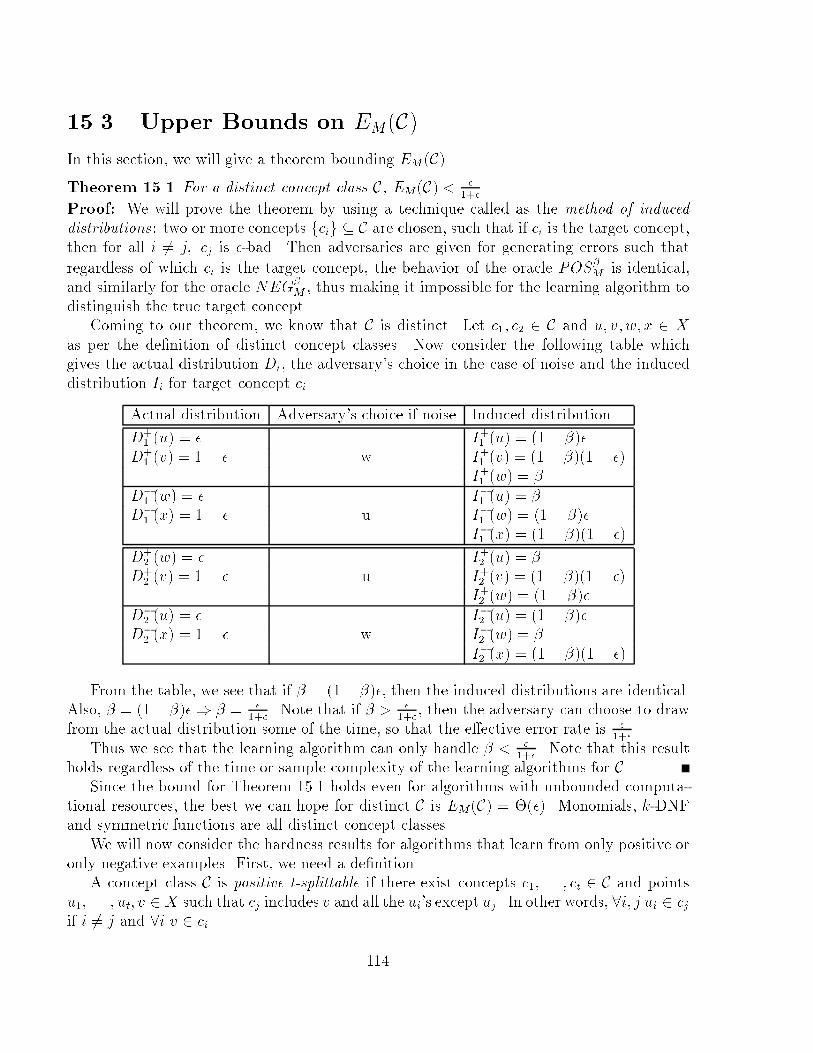
15.3 Upper Bounds on EM(C)
In this section, we will give a theorem bounding EM (C).
Theorem 15.1 For a distinct concept class C, EM(C) < �1+�
.
Proof: We will prove the theorem by using a technique called as the method of induced
distributions: two or more concepts fcig � C are chosen, such that if ci is the target concept,
then for all i 6= j; cj is �-bad. Then adversaries are given for generating errors such that
regardless of which ci is the target concept, the behavior of the oracle POS�M is identical,
and similarly for the oracle NEG�M , thus making it impossible for the learning algorithm to
distinguish the true target concept.
Coming to our theorem, we know that C is distinct. Let c1; c2 2 C and u; v; w; x 2 X
as per the de�nition of distinct concept classes. Now consider the following table which
gives the actual distribution Di, the adversary's choice in the case of noise and the induceddistribution Ii for target concept ci.
Actual distribution Adversary's choice if noise Induced distribution
D+1 (u) = � I+1 (u) = (1� �)�
D+1 (v) = 1 � � w I+1 (v) = (1 � �)(1� �)
I+1 (w) = �
D�1 (w) = � I�1 (u) = �
D�1 (x) = 1� � u I�1 (w) = (1 � �)�
I�1 (x) = (1� �)(1� �)
D+2 (w) = � I+2 (u) = �
D+2 (v) = 1 � � u I+2 (v) = (1 � �)(1� �)
I+2 (w) = (1 � �)�
D�2 (u) = � I�2 (u) = (1� �)�
D�2 (x) = 1� � w I�2 (w) = �
I�2 (x) = (1� �)(1� �)
From the table, we see that if � = (1� �)�, then the induced distributions are identical.Also, � = (1� �)�) � = �
1+�. Note that if � > �
1+�, then the adversary can choose to draw
from the actual distribution some of the time, so that the e�ective error rate is �1+�
.
Thus we see that the learning algorithm can only handle � < �1+�
. Note that this result
holds regardless of the time or sample complexity of the learning algorithms for C.Since the bound for Theorem 15.1 holds even for algorithms with unbounded computa-
tional resources, the best we can hope for distinct C is EM(C) = �(�). Monomials, k-DNF
and symmetric functions are all distinct concept classes.
We will now consider the hardness results for algorithms that learn from only positive or
only negative examples. First, we need a de�nition.
A concept class C is positive t-splittable if there exist concepts c1; . . . ; ct 2 C and pointsu1; . . . ; ut; v 2 X such that cj includes v and all the ui's except uj. In other words, 8i; j ui 2 cjif i 6= j and 8i v 2 ci.
114
As an example, monomials on n variables are positive n-splittable. Let c1 = x1; . . . ; cn =
xn and let u1 = 011 . . . 11; u2 = 101 . . . 11; . . . ; un = 111 . . . 10; v = 111 . . . 11. Also, if C is a
concept class with vcd(C) = d, then C is both positive and negative d-splittable.
Theorem 15.2 For positive t-splittable C, any algorithm calling on POS�M can tolerate an
error rate � � �t�1
regardless of time or sample complexity.
Proof: The theorem is proved using the method of induced distributions. Since C is positive
t-splittable, let c1; . . . ; ct 2 C and u1; . . . ; ut; v 2 X be as in the de�nition of positive t-
splittable. Let cj be the target concept. Consider the following actual distribution:
D+j (v) = 1 � �
D+j (ui) = �
t�18i 6= j
D�j (uj) = 1
In case of noise, the adversary chooses uj. Thus, the induced distribution is
I+j (v) = (1� �)(1� �)
I+j (ui) = (1� �)�
�t�1
�8i 6= j
I+j (uj) = �
If � = (1 � �)�
�t�1
�, then the induced distributions I+j are identical for all ui. Solving
for �, we get
� =�
t�1
1 + �t�1
=�
t� 1 + �
��
t� 1
Thus we see that the learning algorithm can only tolerate an error rate of � < �t�1
.
The above theorem leads to the following corollaries.
Corollary 15.1 A learning algorithm for monomials (using only positive or only negativeexamples) can tolerate an error rate of � < �
n�1where n is the number of variables in the
monomial.
Corollary 15.2 A learning algorithm for k-DNF (using only positive or only negative ex-amples) can tolerate an error rate of � < c0�
nkwhere c0 is a constant > 0.
Corollary 15.3 A learning algorithm for symmetric functions (using only positive or only
negative examples) can tolerate an error rate of � < �n�1
where n is the number of variablesin the symmetric functions.
115
The above corollaries agree with some earlier work by Valiant [44]. Valiant proved the
following two theorems.
Theorem 15.3 Monomials are learnable using calls to POS�M for � � c0�
nfor constant c0.
The learning algorithm for the above is slightly di�erent from the algorithm for learning
monomials in a noise-free environment. In this case, variable xi is deleted from the current
hypothesis only if xi = 0 in at least 2c0�n
of the examples seen so far.
Theorem 15.4 k-DNF is learnable using calls to NEG�M for � � c0�
nkfor constant c0.
15.4 Generalization of Occam's Razor
In the previous section, we saw the limitations on the error rate that a learning algorithmcan tolerate, even if it had unbounded computational resources. In this section, we willconcentrate on the largest error rate that a polynomial time learning algorithm can tolerate.
We will give a technique for building robust algorithms which is a generalization of Occam'sRazor.
Let A be an algorithm accessing POS�M and NEG
�M , and taking inputs � > 0; � < 1.
Suppose that for target concept c 2 C and 0 � � < �4; A makes m calls to POS�M and
receives examples u1; . . . ; um, and m calls to NEG�M and receives examples v1; . . . ; vm, and
outputs hA 2 H satisfying with probability at least 1 � �:
(i)fui : ui 62 hAg
m��
2
(ii)fvi : vi 2 hAg
m��
2Thus, with high probability, hA agrees with a fraction of at least 1 � �
2of the sample. Such
an algorithm A will be called a �-robust Occam Algorithm for C.
Theorem 15.5 Let � < �4, and let A be a �-robust Occam Algorithm for C outputting
hA 2 H. Then A is a PAC-learning algorithm for C for m = O�1�
ln 1�
+ 1�
ln jHj�.
Proof: We will show that if condition (i) holds for A, then e+(hA) < �, and similarly, of
condition (ii) holds, then e�(hA) < �.
Suppose h 2 H is �-bad, i.e. e+(h) � �. Then, the probability that h agrees with anexample x from POS
�M is at most
(1� �)(1� �) + � � 1�3�
4
for � < �4. Thus, the probability that h agrees with at least a fraction 1� �
2of the m positive
examples is
LE
�3�
4;m;
�
2m
�� e�m�=24
116
using Cherno� bounds. Thus, the probability that some �-bad h agrees with a fraction 1� �2
of the m positive examples is at most
jHje�m�=24:
We want this to be at most �2. Thus, by solving
jHje�m�=24 ��
2
for m, we get
m �24
�
�ln jHj+ ln
2
�
�
On the other hand, if c is the target concept, then the probability that c does not agreewith a fraction 1� �
2of the m positive examples is
GE
��
4;m;
�
2m
���
2
for � � �4
and m from above. Observe that m = O�1�
ln 1�
+ 1�
ln jHj�. Also, for such an m,
any hypothesis agreeing with a fraction 1 � �2
of a sample of size m from POS�M must have
e+(h) < � with high probability.The above theorem can be used to prove the correctness of the following learning algo-
rithms by Valiant [44].
Theorem 15.6 There is a polynomial time learning algorithm A for monomials which canlearn from positive examples and tolerate an error rate of �
��n
�where n is the number of
variables in the monomial.
Theorem 15.7 There is a polynomial time learning algorithm A for k-DNF which can learnfrom negative examples and tolerate an error rate of �
��nk
�where n is the number of variables
in the k-DNF formula.
15.5 Using Positive and Negative Examples to Im-
prove Learning Algorithms
In this section, we show that by using both positive and negative examples, we can improve
the noise rate that can be handled by the learning algorithm.
Theorem 15.8 Let C be a polynomial time learnable concept class in the error-free modelby algorithm A with sample complexity sA(�; �; n) and let s = sA( �
8; 12; n). Then, we can learn
C in polynomial time with an error rate of � = �min
��8; ln s
s
��.
117
Proof: Assume � < ln ss
. Run algorithm A using oracles POS�M and NEG�M with accuracy
set to �8
and con�dence set to 12. The probability that no errors occur during this run of A is
(1� �)s �
1 �
ln s
s
!s
=
0@ 1�
ln s
s
! sln s
1A
ln s
Recall that
ex = O(1 + x)
Putting x = � ln ss
, we get
e�ln ss = O
1 �
ln s
s
!
which implies
e�1 =�e�
ln ss
� sln s
= O
0@
1�ln s
s
! sln s
1A
Thus, we get
(1� �)s� O
�e� ln s
�
= O
�1
s
�
Let a successful run be one that has no errors. Using Cherno� bounds, it can be shownthat for r = O
�s ln 1
�
�, the probability of no successful runs in r tries is at most �
2.
Thus, by running algorithm A r times, we get hypotheses h1; . . . ; hr, one of which is�8-good. By doing our standard hypothesis testing, we can �nd this hypothesis. Note that if
a hypothesis is �8-good, then regardless of what the adversary does, we get an error rate of
at most (1��) �8
+� � �8
for the range of � we are assuming. Thus, we can use the standard
hypothesis testing.Earlier, we saw that polynomial time algorithms for learning monomials using only pos-
itive examples can tolerate an error rate of ���n
�. Applying the above theorem improves
this bound by a log factor as can be seen in the following corollary.
Corollary 15.4 There is a polynomial time learning algorithm A for monomials which can
learn from both positive and negative examples and tolerate an error rate of ��n
ln n�
�where
n is the number of variables in the monomial.
Also, in an earlier topic, we saw that any learning algorithm A for a concept class C must
have sample complexity
sA(�; �) =
1
�ln
1
�+d
�
!
118
where d = vcd(C). Applying Theorem 15.8, we get an algorithm for C that can tolerate a
malicious error rate of c0�ln d
�
��d
for a constant c0. Note that Corollary 15.4 follows from
this more general result since the VC dimension of monomials is �(n).
15.6 Relationship between Learning Monomials with
Errors and Set Cover
In this section, we will generalize the Set Cover problem to Partial Cover and show its
relationship to learning monomials with errors. We �rst de�ne the partial cover problem.
Problem: PC (Partial Cover)
Instance: Finite sets S1; . . . ; Sn, (without loss of generality, assume [ni=1Si = f1; . . . ;mg),positive real costs c1; . . . ; cn, and a positive fraction 0 < p � 1.Output: J 0 � f1; . . . ; ng such that j[j2J 0Sjj � pm and PCcost(J 0) =
Pj2J 0 cj is minimized.
The Partial Cover Problem is clearly NP-complete, since it contains set cover as a special
case (p = 1). We now give the greedy approximation algorithm for Partial Cover.Let J = f1; . . . ; ng and T = f1; . . . ;mg.
Algorithm G for the Partial Cover Problem:
0. Set J� = 0;m = j [j2J 0 Sjj.
1. Let q = pm � j [j2J� Sjj: 8j 62 J�, if jSjj > q, delete any jSjj � q elements from Sj.
2. If j [j2J 0 Sjj � pm then stop: J� is a partial cover. Otherwise �nd a k maximizing the
ratio jSk j
ck.
3. Add k to J�, and replace each Sj by Sj � Sk. Return to Step 1.
It can be shown that G gives a cover which is within �(logm) of the optimal. Thefollowing theorem demonstrates that an approximation algorithm for a covering problemcan be used to obtain a robust algorithm for monomials. See the Kearns and Li paper for
both of these proofs.
Theorem 15.9 There is a polynomial time learning algorithm A for monomials of length
at most l which can tolerate an error rate of c0�l
�1
log l ln n�
�where n is the number of variables
in the monomial and c0 is a positive constant.
Now we shall show that by approaching the best known upper bound of � on EM (Mn),
where Mn is the class of monomials over n variables, we are actually improving the bestknown approximation algorithms for set cover.
119
Theorem 15.10 Suppose A is a polynomial time learning algorithm for learning monomials
using monomials, and can tolerate a malicious error rate of � = �r(n)
, then there is a poly-
nomial time algorithm A0 for set cover that �nds a weighted cover with cost at most 4r(n)
times the optimal cost, where n is the number of sets.
Proof: We will give a reduction showing how algorithm A can be used as a subroutine to
obtain the desired set cover approximation algorithm by associating the weighted set covers
with monomials. Let Jopt 2 f1; . . . ; ng be an optimal cover of T = f1; . . . ;mg, and let
PCcost(Jopt) = CPCopt. Each cover fi1; . . . ; ilg is associated with monomial xi1 ^ . . . ^ xil.Let Mopt be the monomial corresponding to the optimal cover Jopt. The basic idea is for A0
to run A with Mopt as the target concept. We then force the output of algorithm A to be a
monomial with error close to Mopt. This monomial will correspond to a cover that is close
to optimal.
We will use NEG�M to force the output of A to correspond to a cover. To achieve this goal
we put a uniform distribution over the following set of m negative examples. For each i 2 T ,de�ne ~ei to be an n-bit vector whose jth bit is 0 if and only if i 2 Sj . For example, let m = 5and S1 = f1; 3; 5g, S2 = f1; 2g, S3 = f1; 4; 5g, and S4 = f1; 3g. Then ~e1 = 0000, ~e2 = 1011,~e3 = 0110, ~e4 = 1101, and ~e5 = 0101. Let E = [i2T ~ei. Observe that J 0 = fi1; . . . ; ilgis a cover of T if and only if every vector in E is a negative example of the corresponding
monomial. Thus since Jopt is a cover, Mopt is consistent with all the negative examples.Finally, we let � < 1
m. Note that 1
�is polynomial in the size of the set cover instance. Since
we force A to output a monomial consistent with the sample, A0 outputs a cover. Note thatat this point we have used the assumption that A learns monomials by monomials becausewe do not have a natural mapping between non-monomials and possible covers.
Next we use POS�M to force the cost of the cover to be low. First, without loss of
generality, we assume the costs are scaled so thatPn
i=1 ci ��
r(n)< 1. Next we de�ne the
induced distribution I+ on the positive examples. We will then show that this distribution
can be obtained. For each 1 � i � n, let ~pi be the n-bit vector that is 1 everywhere exceptin the ith position. Now I+ places a probability of ci on all ~pi, and probability 1 �
Pni=1 ci
on ~1n. The probability that a monomial xi1 ^ . . . ^ xil disagrees with a positive example isPlk=1 cik = COST(J) where J = fi1; . . . ; ilg is the corresponding cover.
Thus, the smallest possible rate of disagreements with I+ is CPCopt and is achieved by
Mopt. Since CPCopt �Pn
i=1 ci ��
r(n)= �, this distribution can be induced by a malicious
oracle.A good hypothesis output by algorithm A must have a rate of disagreement of at most
2� with Mopt on I+. One factor of � comes from the disagreement with D+, and the other
factor comes from the error � < � induced by the malicious oracle. Finally, we do not know
the actual value of CPCopt. So, we repeatedly divide � by 2 and run A with the new valueof �, but without changing I+. This forces A to output better and better monomials, untilit reaches a point where CPCopt <
�r(n)� 2CPCopt. At that point, the hypothesis output will
have error < 2� � 4r(n)�.
The only problem with this occurs when CPCopt is extremely small causing exponentialnumber of iterations of A. This can be avoided by �rst using the greedy approximation
120
algorithm G and discarding all the sets whose cost is higher than the greedy cover. This
ensures that in the new (smaller) instance, all the costs are polynomially related (within a
multiplicative logm factor), and thus we can maintain the polynomial running time.If in the above theorem, r(n) = o(log n), then A would imply a signi�cant improvement
in the existing approximation for set cover. As for our learning problem, the only other
alternative (besides improving on the best known set covering result) is to use a hypothesis
space larger than just monomials.
121

122
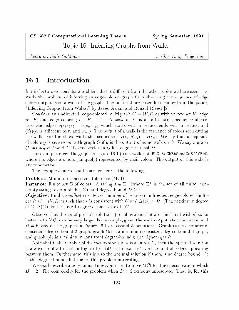
CS 582T Computational Learning Theory Spring Semester, 1991
Topic 16: Inferring Graphs from Walks
Lecturer: Sally Goldman Scribe: Andy Fingerhut
16.1 Introduction
In this lecture we consider a problem that is di�erent from the other topics we have seen|we
study the problem of inferring an edge-colored graph from observing the sequence of edge
colors output from a walk of the graph. The material presented here comes from the paper,\Inferring Graphs From Walks," by Javed Aslam and Ronald Rivest [9].
Consider an undirected, edge-colored multigraph G = (V;E; c) with vertex set V , edgeset E, and edge coloring c : E ! �. A walk on G is an alternating sequence of ver-
tices and edges v1e1v2e2 . . .vnenvn+1 which starts with a vertex, ends with a vertex, and(8i)(ei is adjacent to vi and vi+1). The output of a walk is the sequence of colors seen duringthe walk. For the above walk, this sequence is c(e1)c(e2) . . . c(en). We say that a sequenceof colors y is consistent with graph G if y is the output of some walk on G. We say a graphG has degree bound D if every vertex in G has degree at most D.
For example, given the graph in Figure 16.1 (b), a walk is AaBbCcAcCbBbCcAdCeBfAfBeC,where the edges are here (uniquely) represented by their colors. The output of this walk is
abccbbcdeffe.The key question we shall consider here is the following:
Problem: Minimum Consistent Inference (MCI)Instance: Finite set � of colors. A string s 2 �+ (where �+ is the set of all �nite, non-empty strings over alphabet �), and degree bound D � 2.Objective: Find a smallest (i.e. fewest number of vertices) undirected, edge-colored multi-
graph G = (V;E; c) such that s is consistent with G and �(G) � D. (The maximum degreeof G, �(G), is the largest degree of any vertex in G).
Observe that the set of possible solutions (i.e. all graphs that are consistent with s) to aninstance to MCI can be very large. For example, given the walk output abccbbcdeffe, andD = 6, any of the graphs in Figure 16.1 are candidate solutions. Graph (a) is a minimum
consistent degree-bound 2 graph, graph (b) is a minimum consistent degree-bound 4 graph,
and graph (d) is a minimum consistent degree-bound 6 (or higher) graph.
Note that if the number of distinct symbols in s is at most D, then the optimal solutionis always similar to that in Figure 16.1 (d), with exactly 2 vertices and all edges appearingbetween them. Furthermore, this is also the optimal solution if there is no degree bound|it
is this degree bound that makes this problem interesting.
We shall describe a polynomial time algorithm to solve MCI for the special case in which
D = 2. The complexity for the problem when D > 2 remains unresolved. That is, for this
123
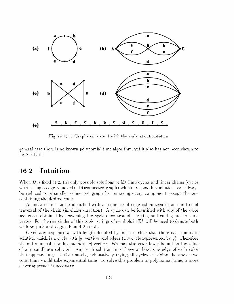
Figure 16.1: Graphs consistent with the walk abccbbcdeffe.
general case there is no known polynomial time algorithm, yet it also has not been shown tobe NP-hard.
16.2 Intuition
When D is �xed at 2, the only possible solutions to MCI are cycles and linear chains (cycleswith a single edge removed). Disconnected graphs which are possible solutions can alwaysbe reduced to a smaller connected graph by removing every component except the onecontaining the desired walk.
A linear chain can be identi�ed with a sequence of edge colors seen in an end-to-end
traversal of the chain (in either direction). A cycle can be identi�ed with any of the color
sequences obtained by traversing the cycle once around, starting and ending at the samevertex. For the remainder of this topic, strings of symbols in �+ will be used to denote bothwalk outputs and degree bound 2 graphs.
Given any sequence y, with length denoted by jyj, it is clear that there is a candidatesolution which is a cycle with jyj vertices and edges (the cycle represented by y). Therefore
the optimum solution has at most jyj vertices. We may also get a lower bound on the value
of any candidate solution. Any such solution must have at least one edge of each colorthat appears in y. Unfortunately, exhaustively trying all cycles satisfying the above two
conditions would take exponential time. To solve this problem in polynomial time, a more
clever approach is necessary.
124
Although the smallest degree 2 graph consistent with a walk is often a cycle (and certainly
can always be made into a cycle), it is useful to �rst consider the problem of �nding the
smallest chain consistent with a given walk. We can then use the ideas developed for this
simpler problem to solve the more general problem.
Consider the sequence y =baabcddccde. The smallest chain which is consistent with it
is z =abcde. In general, how can we get from y to z? Looking at the substring cddccd, we
see that it is of the form xxRx where x = cd (xR denotes the reverse of string x). Such a
substring can be thought of as a portion of the walk which traverses consecutive edges in x,
then goes back over them in reverse, and then forward again. If xxRx is replaced by x, then
that portion of the walk still starts and ends at the same vertices. Therefore, the shorter
string represents a smaller chain that is still consistent with the original walk. Furthermore,
observe that a pre�x of the string is baab. This is of the form xRx where x = ab. By
replacing this with x, the result is a shorter sequence representing a smaller chain. Theoriginal sequence is still a walk on this graph; it merely starts at a di�erent vertex. Similartransformations can be performed on a su�x.
This suggests the following approach to solving the problem of inferring a minimumlength linear chain consistent with a walk. Starting with the walk output given, applyreductions of the above forms until it is no longer possible. Now, one may (and should) askthemselves a few questions about the usefulness of this approach. Is it possible for more thanone reduction to be applicable to a sequence? If so, are all resulting strings consistent withthe original walk? Furthermore, which order of application leads to the optimal solution (i.e.
the shortest linear chain)? In other words, for a given order of application what guaranteesthat the resulting string is both consistent and optimal?
To answer the �rst question, it is possible for more than one reduction to be applicable,
as exhibited by the sequence abbbccbbbbc. Figure 16.2 shows all possible reductions ofthe form xxRx ! x that can be performed on this sequence. Since there may be morethan one reduction possible on a sequence, which one should be chosen? In the example ofFigure 16.2, it does not seem to matter which reductions are performed �rst. The eventualresult of continuing reductions until no more are possible is always abc. So in this case, the
order of reductions does not matter, and thus any applicable reduction can be applied. Ingeneral, does performing any applicable reduction lead to a consistent and optimal solution?
We shall prove that for this problem the order of reductions does not matter. Such questions
have been asked in other contexts for other kinds of reductions. See the Aslam, Rivestpaper [9] for references.
16.3 Preliminaries
Before proving that any order of reductions produces a consistent and optimal linear chain,we �rst need some de�nitions.
Let S be a set. A binary relation on S is a subset of S � S. Let ! be a binary relation
on S. If (x; y) 2!, we write x! y.Let � be the identity relation on S, � = f(x; x)jx 2 Sg. Given two binary relations!A and
125
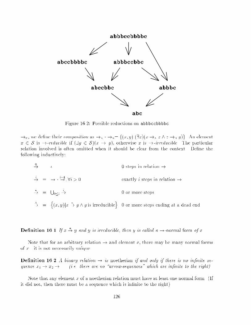
Figure 16.2: Possible reductions on abbbccbbbbc
!B, we de�ne their composition as !A � !B= f(x; y)j(9z)(x!A z ^ z !B y)g. An element
x 2 S is !-reducible if (9y 2 S)(x ! y), otherwise x is !-irreducible. The particularrelation involved is often omitted when it should be clear from the context. De�ne thefollowing inductively:
0! = � 0 steps in relation !
i! = ! �
i�1! ;8i > 0 exactly i steps in relation !
�! =
S0�i
i! 0 or more steps
^! =
n(x; y)jx
�! y ^ y is irreducible
o0 or more steps ending at a dead end
De�nition 16.1 If x�! y and y is irreducible, then y is called a !-normal form of x.
Note that for an arbitrary relation ! and element x, there may be many normal forms
of x|it is not necessarily unique.
De�nition 16.2 A binary relation ! is noetherian if and only if there is no in�nite se-
quence x1! x2! . . . (i.e. there are no \arrow-sequences" which are in�nite to the right).
Note that any element x of a noetherian relation must have at least one normal form. (Ifit did not, then there must be a sequence which is in�nite to the right).
126
De�nition 16.3 A binary relation ! is con uent if and only if (8w; x; y)(w�! x ^ w
�!
y ) (9z)(x�! z ^ y
�! z)) (i.e., for any element w, if both x and y can be reached from w,
then there is an element z which can be reached from both x and y).
We note that the con uence property is equivalent to the well known Church-Rosser
property.
De�nition 16.4 A binary relation ! is locally con uent if and only if (8w; x; y)(w !x ^w! y) (9z)(x
�! z ^ y
�! z)) (i.e., for any element w, if both x and y are immediate
successors of w, then there is an element z which can be reached from both x and y).
The following well known results (they can be found in Huet [23]) will be very useful
here.
Theorem 16.1 A noetherian relation is con uent if and only if it is locally con uent.
Theorem 16.2 If a binary relation is con uent, then the normal form of any element, if it
exists, is unique.
So, for a con uent noetherian relation, every element x has exactly one normal form.Denote this normal form by x.
De�nition 16.5 A binary relation ! is strictly decreasing if (8x; y)(x�! y ) jyj < jxj).
It should be clear that every strictly decreasing relation is noetherian.The way that all of these de�nitions and theorems are used is as follows. For a particular
problem which involves �nding a minimum consistent chain from a given type of walk, �nda relation! on strings such that y
�! z if and only if y is a walk on chain z. Prove that !
is locally con uent and strictly decreasing. The rewards for this work are (1) every string y
has a unique normal form y; (2) the smallest chain consistent with any walk y is y (to be
proven later); (3) an algorithm to �nd y can choose to perform !-reductions in any orderdesired (by con uence).
16.4 Inferring Linear Chains from End-to-end Walks
In this section, we examine the problem of inferring chains from walks. We will furtherrestrict the problem to inferring chains from end-to-end walks, in which it is known that
the walk begins at one end of the chain and stops at the other end. We later consider the
problem of inferring chains from general walks, and then the problem of inferring any degree2 graph from a general walk.
Following the outline at the end of the previous section, de�ne the relation !B on theset �+ as
!B=n
(pxxRxq; pxq)jp; q 2 �� ^ x 2 �+o:
127
It should be clear that if y!B z, then y is an end-to-end walk on z with a single \zig-zag" in
the middle. We now prove that regardless of the order in which!B is applied, the resulting
walk is consistent and that all linear chains consistent with the walk can be obtained in this
manner.
Lemma 16.1 For all y; z 2 �+, y is an end-to-end walk on chain z , y�!B z.
Proof: ()) Since y is an end-to-end walk on the chain z, there is a sequence of vertices
in the chain which can represent that walk. Such an embedding partitions y into segments
that are the portions of y seen between reversals or \folds" in the walk. For example, the
walk abccbbcd on chain abcd can be partitioned into the segments abc, cb, and bcd.
Note that the sequence of segments are alternating \right" and \left" segments, starting
and ending with a \right" segment. Therefore there must be an odd number of segments.Also, the second segment is no longer than the �rst, and the second to last segment is nolonger than the last.
By contradiction, assume that the implication ) is false. Then there is a shortestcounterexample y such that y is an end-to-end walk on some z, but y
�!B z does not hold.
Let s be a shortest segment of an embedding of y into z. There are several cases.
1. The segment s is the only segment. Then y = z and y�!B z holds trivially giving the
desired contradiction.
2. There are several segments, and s is the �rst or last segment. As noted above, we canthen select s to be either the second or second to last segment, respectively, since theyare guaranteed to be no longer than s. Thus this case can be handled using case 3below.
3. There are several segments, and s is a \middle" segment. Since s is a shortest segment,the previous segment ends with sR and the next segment begins with sR. Thus y =psRssRq!
BpsRq. There are two subcases.
(a) psRq�!B z. Then y
�!B z giving the desired contradiction.
(b) psRq�!B z does not hold. Then psRq, which is clearly also a walk on z, is a
shorter counterexample than y giving a contradiction.
(() Easily proven by induction on the number of \steps" in the relation !B between y
and z, given the observation immediately preceding the lemma.
It should be clear that !B is strictly decreasing. Every !B-reduction removes at least
two symbols from a string. Thus to prove that !B is con uent we need just show that it islocally con uent.
Lemma 16.2 The relation !B is locally con uent.
128
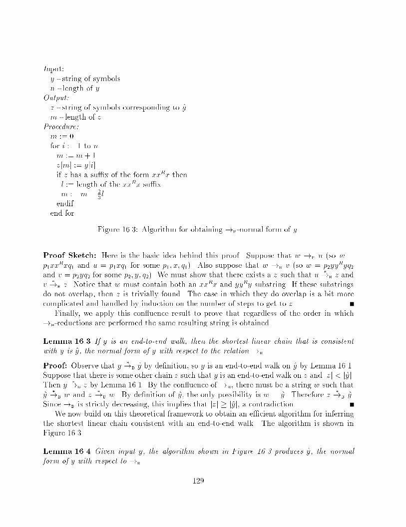
Input:
y - string of symbols
n - length of y
Output:
z - string of symbols corresponding to y
m - length of z
Procedure:
m := 0
for i := 1 to n
m := m+ 1
z[m] := y[i]
if z has a su�x of the form xxRx thenl := length of the xxRx su�xm := m� 2
3l
endifend for
Figure 16.3: Algorithm for obtaining !B-normal form of y.
Proof Sketch: Here is the basic idea behind this proof. Suppose that w !B u (so w =
p1xxRxq1 and u = p1xq1 for some p1; x; q1). Also suppose that w !B v (so w = p2yy
Ryq2and v = p2yq2 for some p2; y; q2). We must show that there exists a z such that u
�!B z and
v�!B z. Notice that w must contain both an xxRx and yyRy substring. If these substrings
do not overlap, then z is trivially found. The case in which they do overlap is a bit morecomplicated and handled by induction on the number of steps to get to z.
Finally, we apply this con uence result to prove that regardless of the order in which!B-reductions are performed the same resulting string is obtained.
Lemma 16.3 If y is an end-to-end walk, then the shortest linear chain that is consistentwith y is y, the normal form of y with respect to the relation !B.
Proof: Observe that y�!B y by de�nition, so y is an end-to-end walk on y by Lemma 16.1.
Suppose that there is some other chain z such that y is an end-to-end walk on z and jzj < jyj.Then y
�!B z by Lemma 16.1. By the con uence of !B, there must be a string w such that
y�!B w and z
�!B w. By de�nition of y, the only possibility is w = y. Therefore z
�!B y.
Since!B is strictly decreasing, this implies that jzj � jyj, a contradiction.
We now build on this theoretical framework to obtain an e�cient algorithm for inferring
the shortest linear chain consistent with an end-to-end walk. The algorithm is shown inFigure 16.3.
Lemma 16.4 Given input y, the algorithm shown in Figure 16.3 produces y, the normal
form of y with respect to !B.
129
Proof: Let zi be the value of z after the ith iteration of the for loop has completed. Clearly
y�!B z holds. Now we show that zi is !B-irreducible for all i by induction. The basis that
z1 is irreducible is obvious; it consists of only a single symbol. Now for all i > 1, we need to
show that zi�1 is irreducible implies that zi is irreducible. There are two cases.
1. A su�x of the form xxRx was found. In this case, zi is a proper pre�x of zi�1.
Therefore, if zi�1 is irreducible (i.e., contains no substrings of the form xxRx), then ziis irreducible.
2. No su�x of the form xxRx was found. In this case, zi is zi�1 plus a single symbol
appended to the end. Suppose zi is reducible. Then it must contain a substring of the
form xxRx. There are two subcases.
(a) The substring ends at the last symbol of zi. This cannot be the case, however,since such a su�x was not found by the algorithm.
(b) The substring ends before the last symbol of zi. This is also impossible, for thenzi�1 would be reducible.
We conclude that zi is irreducible.If the search for the su�x is done in an obvious, exhaustive manner, then it requires
O(i2) time for a string of length i. The worst case behavior of the algorithm occurs whenthe input string y is irreducible. It then requires O(n3) time.
16.5 Inferring Linear Chains from General Walks
Before returning to the problem of inferring a linear chain from a walk, we �rst consider theproblem of inferring a linear chain from a general walk (as opposed to an end-to-end walk).
A walk an a linear chain z is a sequence of colors corresponding to the edges traversed insome walk on z that begins a some vertex vi and at some point passes through both theleftmost and rightmost vertices of the chain.
Observe that embedded in the general walk of the chain there must be an end-to-endwalk. The approach used here is just an extension of the approach seen in the last section.
However, now we must have special reductions to handle the head and the tail of the walk.Following the de�nition of !B, we de�ne the following relation !H on the set �+ as
!H=n
(xRxq; xq)jq 2 �� ^ x 2 �+o:
Likewise we de�ne the relation !T on the set �+ as
!T=n
(pxxR; px)jp 2 �� ^ x 2 �+o:
Finally, we de�ne
!HBT=!B
[!H
[!T :
130
Then proceeding in a very similar fashion as in the last section it can be shown that
the binary relation !HBT is con uent. This property can be used to prove the following key
theorem.
Theorem 16.3 If y is a walk, then the shortest linear chain that can produce y is y, the
normal form of y with respect to the relation !HBT.
See the Aslam, Rivest paper [9] for the details of these proofs.
To further simplify the algorithm it would be nice if we could perform the three type of
reductions one at a time. We now prove that this approach can be applied.
Lemma 16.5 If w^!B x
^!H y
^!T z, then z is the normal form of w with respect to the
relation !HBT.
Proof: Clearly, we have that w�!B x
�!H y
�!T z ) w
�!HBT z. Thus we need just show
that z is irreducible under !HBT. Clearly z is irreducible under !T. Also z is a pre�x ofy by the de�nition of !T. Suppose that z is not irreducible under !H, but then y is notirreducible under !H which contradicts the de�nition of
^!H. Furthermore, note that z is
a substring of x by the de�nitions of !H and !T. Suppose z is not irreducible under !B.
Then x is not irreducible under !B contradicting the de�nition of^!B. Thus z is irreducible
under !B, !H, and !T, and hence irreducible under !HBT.So putting these ideas all together, to obtain an algorithm for inferring a linear chain
from a general walk w we can just perform the following steps:
1. x normal-form of w with respect to !B
2. y normal-form of x with respect to !H
3. z normal-form of y with respect to !T
It then follows from the above results that z is the normal form of w with respect to !HBT.All that remains is to give an algorithm to �nd the normal form of a string with respectto !H and !T. See Figure 16.4 for an algorithm to �nd the normal form of a string with
respect to !T. Clearly a similar algorithm can be given to �nd the normal form of a stringwith respect to!H. The proof of correctness for the algorithm given in Figure 16.4 is similar
(but easier) than the proof of Lemma 16.4 and is thus omitted here.Finally we analyze the running time of this algorithm for inferring a linear chain from
a general walk. We have already seen that the �rst step can be performed in O(n3) time.
Now we just need to analyze the algorithm given in Figure 16.4. If the input is irreduciblethen O(n2) time is spend trying to �nd a su�x of the form xxR. On the other hand, if the
input is not irreducible O(i2) time is spent �nding each xxR su�x of length 2i or verifyingone does not exist. Thus we get the recurrence
T (n) = maxifT (n� i) +O(i2)g = O(n2):
Thus the overall running time is O(n3).
131
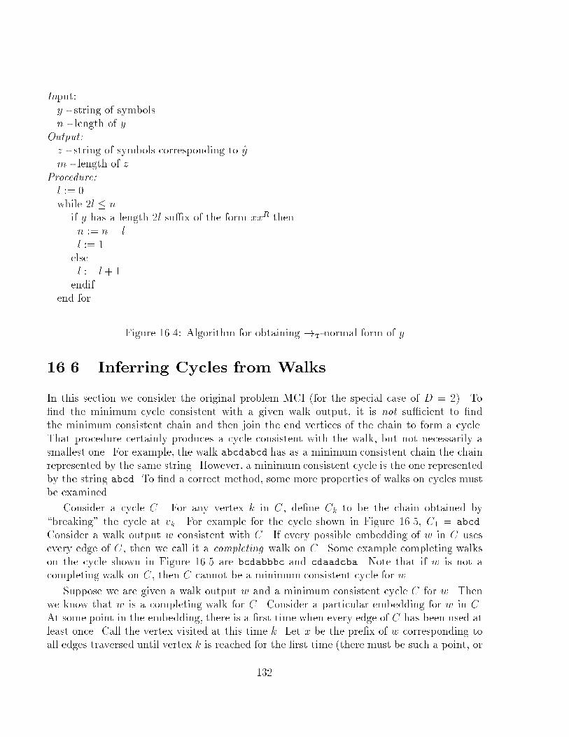
Input:
y - string of symbols
n - length of y
Output:
z - string of symbols corresponding to y
m - length of z
Procedure:
l := 0
while 2l � n
if y has a length 2l su�x of the form xxR then
n := n� ll := 1
elsel := l+ 1
endifend for
Figure 16.4: Algorithm for obtaining !T-normal form of y
16.6 Inferring Cycles from Walks
In this section we consider the original problem MCI (for the special case of D = 2). To�nd the minimum cycle consistent with a given walk output, it is not su�cient to �ndthe minimum consistent chain and then join the end vertices of the chain to form a cycle.
That procedure certainly produces a cycle consistent with the walk, but not necessarily asmallest one. For example, the walk abcdabcd has as a minimum consistent chain the chainrepresented by the same string. However, a minimum consistent cycle is the one representedby the string abcd. To �nd a correct method, some more properties of walks on cycles must
be examined.
Consider a cycle C. For any vertex k in C, de�ne Ck to be the chain obtained by
\breaking" the cycle at vk. For example for the cycle shown in Figure 16.5, C1 = abcd.Consider a walk output w consistent with C. If every possible embedding of w in C uses
every edge of C, then we call it a completing walk on C. Some example completing walks
on the cycle shown in Figure 16.5 are bcdabbbc and cdaadcba. Note that if w is not acompleting walk on C, then C cannot be a minimum consistent cycle for w.
Suppose we are given a walk output w and a minimum consistent cycle C for w. Then
we know that w is a completing walk for C. Consider a particular embedding for w in C.At some point in the embedding, there is a �rst time when every edge of C has been used at
least once. Call the vertex visited at this time k. Let x be the pre�x of w corresponding to
all edges traversed until vertex k is reached for the �rst time (there must be such a point, or
132
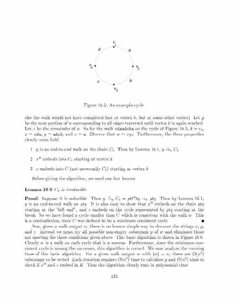
a
bc
d
v4
1v
3v
2v
Figure 16.5: An example cycle.
else the walk would not have completed �rst at vertex k, but at some other vertex). Let ybe the next portion of w corresponding to all edges traversed until vertex k is again reached.Let z be the remainder of w. So for the walk cdaadcba on the cycle of Figure 16.5, k = v2,x = cda, y = adcb, and z = a. Observe that w = xyz. Furthermore, the three propertiesclearly must hold.
1. y is an end-to-end walk on the chain Ck. Thus by Lemma 16.1, y�!B Ck.
2. xR embeds into Ck starting at vertex k.
3. z embeds into C (not necessarily Ck) starting at vertex k.
Before giving the algorithm, we need one last lemma.
Lemma 16.6 Ck is irreducible.
Proof: Suppose it is reducible. Then y�!B Ck = pttRtq !B ptq. Then by Lemma 16.1,
y is an end-to-end walk on ptq. It is also easy to show that xR embeds on the chain ptq
starting at the \left end", and z embeds on the cycle represented by ptq starting at thebreak. So we have found a cycle smaller than C which is consistent with the walk w. This
is a contradiction, since C was de�ned to be a minimum consistent cycle.
Now, given a walk output w, there is no known simple way to discover the strings x, y,and z. Instead we must try all possible non-empty substrings y of w and eliminate those
not meeting the three conditions given above. This basic algorithm is shown in Figure 16.6.
Clearly w is a walk on each cycle that is a success. Furthermore, since the minimum con-
sistent cycle is among the successes, this algorithm is correct. We now analyze the running
time of this basic algorithm. For a given walk output w with jwj = n, there are O(n2)substrings to be tested. Each iteration requires O(n3) time to calculate y and O(n2) time to
check if xR and z embed in K. Thus the algorithm clearly runs in polynomial time.
133
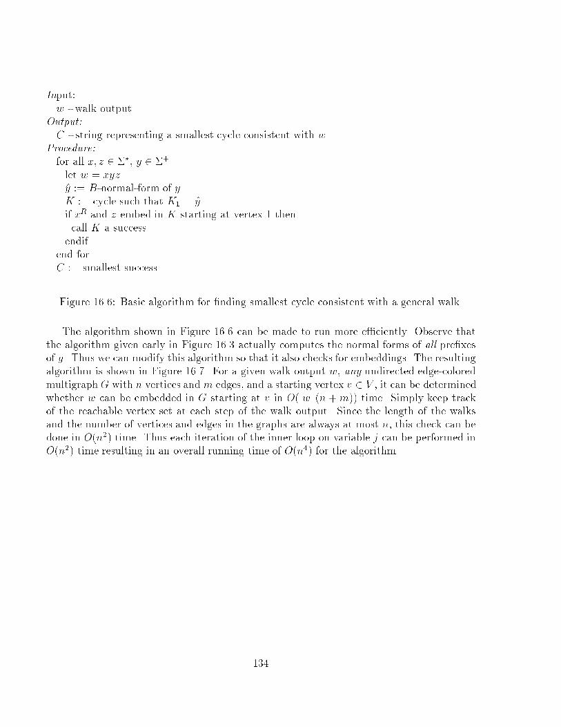
Input:
w - walk output
Output:
C - string representing a smallest cycle consistent with w
Procedure:
for all x; z 2 ��, y 2 �+
let w = xyz
y := B-normal-form of y
K := cycle such that K1 = y
if xR and z embed in K starting at vertex 1 then
call K a success
endifend forC := smallest success
Figure 16.6: Basic algorithm for �nding smallest cycle consistent with a general walk.
The algorithm shown in Figure 16.6 can be made to run more e�ciently. Observe thatthe algorithm given early in Figure 16.3 actually computes the normal forms of all pre�xesof y. Thus we can modify this algorithm so that it also checks for embeddings. The resultingalgorithm is shown in Figure 16.7. For a given walk output w, any undirected edge-colored
multigraphG with n vertices and m edges, and a starting vertex v 2 V , it can be determinedwhether w can be embedded in G starting at v in O(jwj (n + m)) time. Simply keep trackof the reachable vertex set at each step of the walk output. Since the length of the walksand the number of vertices and edges in the graphs are always at most n, this check can bedone in O(n2) time. Thus each iteration of the inner loop on variable j can be performed inO(n2) time resulting in an overall running time of O(n4) for the algorithm.
134
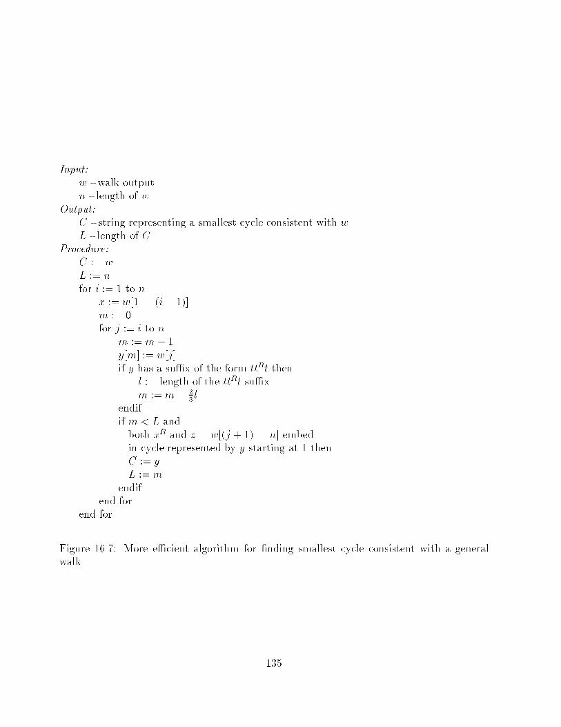
Input:
w - walk output
n - length of w
Output:
C - string representing a smallest cycle consistent with w
L - length of C
Procedure:C := w
L := n
for i := 1 to nx := w[1 . . . (i� 1)]m := 0for j := i to n
m := m+ 1
y[m] := w[j]if y has a su�x of the form ttRt then
l := length of the ttRt su�xm := m� 2
3l
endif
if m < L andboth xR and z = w[(j + 1) . . .n] embedin cycle represented by y starting at 1 thenC := y
L := m
endif
end forend for
Figure 16.7: More e�cient algorithm for �nding smallest cycle consistent with a general
walk.
135

136
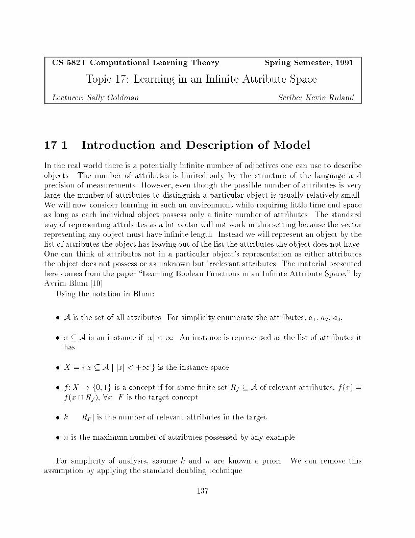
CS 582T Computational Learning Theory Spring Semester, 1991
Topic 17: Learning in an In�nite Attribute Space
Lecturer: Sally Goldman Scribe: Kevin Ruland
17.1 Introduction and Description of Model
In the real world there is a potentially in�nite number of adjectives one can use to describe
objects. The number of attributes is limited only by the structure of the language and
precision of measurements. However, even though the possible number of attributes is verylarge the number of attributes to distinguish a particular object is usually relatively small.We will now consider learning in such an environment while requiring little time and spaceas long as each individual object possess only a �nite number of attributes. The standard
way of representing attributes as a bit vector will not work in this setting because the vectorrepresenting any object must have in�nite length. Instead we will represent an object by thelist of attributes the object has leaving out of the list the attributes the object does not have.One can think of attributes not in a particular object's representation as either attributesthe object does not possess or as unknown but irrelevant attributes. The material presented
here comes from the paper \Learning Boolean Functions in an In�nite Attribute Space," byAvrim Blum [10].
Using the notation in Blum:
� A is the set of all attributes. For simplicity enumerate the attributes, a1, a2, a3,...
� x � A is an instance if jxj <1. An instance is represented as the list of attributes it
has.
� X = fx � A j jxj < +1g is the instance space.
� f :X ! f0; 1g is a concept if for some �nite set Rf � A of relevant attributes, f(x) =f(x \Rf ), 8x. F is the target concept.
� k = jRF j is the number of relevant attributes in the target.
� n is the maximum number of attributes possessed by any example.
For simplicity of analysis, assume k and n are known a priori. We can remove this
assumption by applying the standard doubling technique.
137
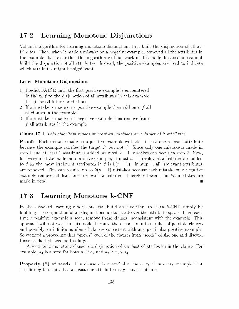
17.2 Learning Monotone Disjunctions
Valiant's algorithm for learning monotone disjunctions �rst built the disjunction of all at-
tributes. Then, when it made a mistake on a negative example, removed all the attributes in
the example. It is clear that this algorithm will not work in this model because one cannot
build the disjunction of all attributes. Instead, the positive examples are used to indicate
which attributes might be signi�cant.
Learn-Monotone Disjunctions
1. Predict FALSE until the �rst positive example is encountered.
Initialize f to the disjunction of all attributes in this example.
Use f for all future predictions.
2. If a mistake is made on a positive example then add onto f allattributes in the example.
3. If a mistake is made on a negative example then remove from
f all attributes in the example.
Claim 17.1 This algorithm makes at most kn mistakes on a target of k attributes.
Proof: Each mistake made on a positive example will add at least one relevant attributebecause the example satis�es the target F but not f . Since only one mistake is made instep 1 and at least 1 attribute is added, at most k � 1 mistakes can occur in step 2. Now,for every mistake made on a positive example, at most n� 1 irrelevant attributes are addedto f so the most irrelevant attributes in f is k(n � 1). In step 3, all irrelevant attributes
are removed. This can require up to k(n� 1) mistakes because each mistake on a negativeexample removes at least one irrelevant attributes. Therefore fewer than kn mistakes aremade in total.
17.3 Learning Monotone k-CNF
In the standard learning model, one can build an algorithm to learn k-CNF simply bybuilding the conjunction of all disjunctions up to size k over the attribute space. Then each
time a positive example is seen, remove those clauses inconsistent with the example. This
approach will not work in this model because there is an in�nite number of possible clausesand possibly an in�nite number of clauses consistent with any particular positive example.
So we need a procedure that \grows" each of the clauses from \seeds" of size one and discardthose seeds that become too large.
A seed for a monotone clause is a disjunction of a subset of attributes in the clause. Forexample, a4 is a seed for both a1 _ a4 and a2 _ a3 _ a4.
Property (*) of seeds If a clause c is a seed of a clause cF then every example that
satis�es cF but not c has at least one attribute in cF that is not in c.
138
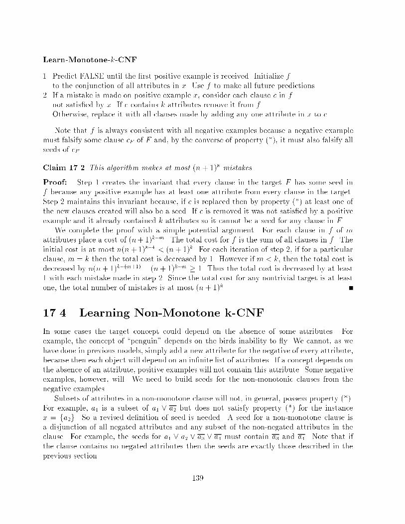
Learn-Monotone-k-CNF
1. Predict FALSE until the �rst positive example is received. Initialize f
to the conjunction of all attributes in x. Use f to make all future predictions
2. If a mistake is made on positive example x, consider each clause c in f
not satis�ed by x. If c contains k attributes remove it from f .
Otherwise, replace it with all clauses made by adding any one attribute in x to c.
Note that f is always consistent with all negative examples because a negative example
must falsify some clause cF of F and, by the converse of property (*), it must also falsify all
seeds of cF .
Claim 17.2 This algorithm makes at most (n+ 1)k mistakes.
Proof: Step 1 creates the invariant that every clause in the target F has some seed inf because any positive example has at least one attribute from every clause in the target.
Step 2 maintains this invariant because, if c is replaced then by property (*) at least one ofthe new clauses created will also be a seed. If c is removed it was not satis�ed by a positiveexample and it already contained k attributes so it cannot be a seed for any clause in F .
We complete the proof with a simple potential argument. For each clause in f of mattributes place a cost of (n+ 1)k�m. The total cost for f is the sum of all clauses in f . The
initial cost is at most n(n+ 1)k�1 < (n+ 1)k. For each iteration of step 2, if for a particularclause, m = k then the total cost is decreased by 1. However if m < k, then the total cost isdecreased by n(n+ 1)k�(m+1) � (n+ 1)k�m � 1. Thus the total cost is decreased by at least1 with each mistake made in step 2. Since the total cost for any nontrivial target is at leastone, the total number of mistakes is at most (n+ 1)k.
17.4 Learning Non-Monotone k-CNF
In some cases the target concept could depend on the absence of some attributes. Forexample, the concept of \penguin" depends on the birds inability to y. We cannot, as we
have done in previous models, simply add a new attribute for the negative of every attribute,because then each object will depend on an in�nite list of attributes. If a concept depends on
the absence of an attribute, positive examples will not contain this attribute. Some negative
examples, however, will. We need to build seeds for the non-monotonic clauses from thenegative examples.
Subsets of attributes in a non-monotone clause will not, in general, possess property (*).For example, a1 is a subset of a1 _ a2 but does not satisfy property (*) for the instance
x = fa2g. So a revised de�nition of seed is needed. A seed for a non-monotone clause is
a disjunction of all negated attributes and any subset of the non-negated attributes in theclause. For example, the seeds for a1 _ a2 _ a3 _ a4 must contain a3 and a4. Note that if
the clause contains no negated attributes then the seeds are exactly those described in the
previous section.
139
Learn-Non-Monotone-k-CNF
1. Predict FALSE until the �rst positive example is received. Initialize f
to the conjunction of all attributes in x. Use f to make all future predictions.
2. If a mistake made on positive example x, consider each clause c in f
not satis�ed by x. If c contains k attributes remove it from f .
Otherwise, replace it with all clauses made by adding any one attribute in x to c.
3. If a mistake is made on a negative example x, then for each subset
fai1; ai2; . . . ; airg � x, (r � k) add to f the clause (ai1 _ ai2 _ � � � _ air).
Claim 17.3 This procedure makes at most (tk + 1)(n + 1)k mistakes on a k-CNF formula
of t clauses.
Proof Sketch: Similar to the previous proof, step 2 maintains the invariant that once aclause in F has a seed in f it will continue to. Step 3 adds to f a seed for some clause thatpreviously had no seed. So the algorithm makes at most t mistakes on negative examples.
Each mistake on a negative example adds to f at most�n
m
�clauses of m literals for all
m � k. Using the same potential as before, each mistake on a negative example adds a total
cost of at mostkX
m=1
n
m
!(n+ 1)k�m �
kXm=1
(n+ 1)k � k(n+ 1)k:
Since at most t mistakes are made on negative examples the total cost of f will increase byat most tk(n + 1)k for all negative examples. Finally since the initial cost is (n + 1)k andeach positive example reduces the cost by at least one, the total number of mistakes made
is at most (tk + 1)(n+ 1)k.
17.5 Generalized Halving Algorithm
Blum generalizes the halving algorithm of Littlestone to the in�nite attribute model. He
concludes that any concept class in the in�nite-attribute model is learnable in polynomial
number of mistakes if k is �nite. This result ignores possible run time constraints.
De�nition 17.1 For some f 2 C, let fS(x) = f(x \ S).
De�nition 17.2 Given S = fai1; ai2; . . . ; aimg � A let C(k; S) = f fS j f 2 C; jRf j � k g.
So jC(k; S)j is the number of functions in C on at most k relative attributes that di�erover examples whose attributes come from S.
140
Sequential Halving Algorithm(C,k)
1. S fg2. H C(k; S), T fg3. On input x predict according to majority vote on functions in H. If the
prediction is incorrect, remove from H those functions that are incorrect
and let T T [ x. Continue until H is empty.
4. If H is empty, Let S S [ T and go to step 2.
Theorem 17.1 This algorithm makes at most O(k2 lg(knjC(k)j)) mistakes.
Previous knowledge of k can be removed by the standard doubling technique.
17.6 Other Topics
Blum also describes how to combine the ideas of Littlestone's WINNOW1 with this newmodel. This new algorithm makes at most O(k lg n) mistakes on any disjunction of k literals.Although we refer to reader to Blum's paper for the algorithm achieving the O(k lgn) mistakebound, we brie y describe a simple idea to obtain an O(k2 log(kn)) mistake bound. Beginwith a small set of attributes S, say those appearing in the �rst positive example. Next
run WINNOW1 using only the attributes in S. (Note that WINNOW1 must be modi�ed tohandle the concepts \true" and \false".) If more than k log(jSj) mistakes are made then someexample on which a mistake was made has some relevant attribute that was ignored. Finally,just add the at most nk log(jSj) attributes ignored and repeat. This result is particularlyuseful if the target depends on a small number of relevant attributes, each example is fairly
large, and the attribute set is enormous. He extends this idea to learning any k-DNF formulaon t terms with at most O(tk2 log(t+ n)) mistakes.
Finally, Blum also describes how any algorithm that learns in a �nite attribute spaceusing membership queries can be modi�ed to learn in the new model with few additionalmistakes and a small time penalty.
141

142
CS 582T Computational Learning Theory Spring Semester, 1991
Topic 18: The Weighted Majority Algorithm
Lecturer: Sally Goldman Scribe: Marc Wallace
18.1 Introduction
In these notes we study the construction of a prediction algorithm in a situation in which
a learner faces a sequence of trials, with a prediction to be made in each, and the goal of
the learner is to make few mistakes. In particular, consider the case in which the learner
has reason to believe that one of some pool of known algorithms will perform well, butthe learner does not know which one. A simple and e�ective method, based on weightedvoting, is introduced for constructing a compound algorithm in such a circumstance. Thisalgorithm is shown to be robust with respect to errors in the data. We then discuss other
situations in which such a compound algorithm can be applied. The material presented herecomes from the paper \The Weighted Majority Algorithm," by Nick Littlestone and ManfredWarmuth [30].
Before describing the weighted majority algorithm in detail we brie y discuss some learn-ing problems in which the above scenario applies. The �rst case is one that we have seenbefore. Suppose one knows that the correct prediction comes from some target concept se-
lected from some known concept class, then one can apply the weighted majority algorithmwhere each concept in the class is one of the algorithms in the pool. As we shall see forsuch situations, the weighted majority algorithm is just the natural generalization of thehalving algorithm. Another situation in which the weighted majority algorithm can be usedin the situation in which one has a set of algorithms for making predictions, one of which
will work well on a given data set. However, it may be that the best prediction algorithmto use depends on the data set and thus it is not known a priori which algorithm to use.Finally, as we shall discuss in more detail below the weighted majority algorithm can oftenbe applied to help in situations in which the prediction algorithm has a parameter that must
be selected and the best choice for the parameter depends on the target. In such cases one
can build the pool of algorithms by choosing various values for the parameter.The basic idea behind the weighted majority algorithm is to give each algorithm in the
pool the input instance, get all the predictions, combine these into one prediction, and then ifwrong pass that data along to the algorithms in the pool. Observe that the halving algorithm
could be considered as a weak master algorithm by simply taking the majority prediction and
throwing out all bad predictors at each mistake. Unfortunately this algorithm is not robustagainst noise. If one algorithm is perfect, but that source is noisy, then the main algorithm
will reject it and may never converge to one solution (it will run out of algorithms).We de�ne the number of anomalies in a sequence of trials as the least number of inconsis-
tent trials of any algorithm in the pool. Notice if there are any anomalies, then the halving
143
algorithm will fail to converge by eliminating all functions.
18.2 Weighted Majority Algorithm
In this section we introduce the weighted majority algorithm.
Weighted Majority Algorithm (WM)
Initially assign non-negative weights (say 1) to each algorithm in the pool
To make a prediction for an instance:
Let q0 be the total weight of algs that predict 0
Let q1 be the total weight of algs that predict 1
Predict 0 i� q0 � q1If a mistake is made, multiply the weights of the algorithms agreeingwith the incorrect prediction by some �xed non-negative � < 1.
Notice that using � = 0 would yield the halving algorithm. However, it is more interesting
to consider what happens as � ! 1. Suppose the pool is called F , and a given sequence oftrials has m anomalies with respect to F . Then
# mistakes � c(log jF j+m)
where c is some constant dependent on �.In general the maximum number of mistakes will be:
� O(log jF j+m) if one algorithm in F makes at most m mistakes.
� O(log(jF j=k) +m) if each of a set of k algorithms in F makes at most m mistakes.
� O(log(jF j=k) + (m=k)) if the total number of mistakes of a set of k algorithms in F isat most m mistakes.
As an application of WM (weighted majority), we return to the use of WINNOW1 tolearn r-of-k threshold functions. Normally the mistake bound is O(kn log n). However, if the
learner has prior knowledge of a close upper bound for r, the mistake bound can be reducedto br = O(kr log n) by carefully selecting the parameters for WINNOW1. Let Ar denote
the algorithm WINNOW1 with a guess of r. Now any sequence that cannot be representedby an r0-of-k function for r0 � r will fail phenomenally, and make far too many mistakes.However, we can apply WM to the set of algorithms fA2ig for all i satisfying 2i � n. Then
the number of mistakes will be O(log log n+ br) = O(kr log n).Now clearly if the size of our algorithm pool is not polynomial the weighted majority
algorithm is not computationally feasible. Still, many reasonable pools of algorithms will
be of polynomial size, or can be reduced to such without a dramatic increase in the averagenumber of mistakes.
144
18.3 Analysis of Weighted Majority Algorithm
Let A = fA1; . . . ; AjAjg be the pool of algorithms, and wi the weight of Ai. The basic
structure of the proofs that follow will be: First, show that after each trial, if a mistake
occurs then the sum of the weights is decreases by at least a factor of u for some u < 1.
Second, let Winit be the total initial weight and Wfin be a lower bound for the total �nal
weights; then Winitum �Wfin, where m is the number of mistakes. This implies that
m �log Winit
Wfin
log 1u
:
We now prove a general theorem bounding the number of mistakes made by the weighted
majority algorithm. We can then apply to obtain the three results given above.
Theorem 18.1 Let S be a sequence of instances and mi the number of mistakes made byAi on S. Let m be the number of mistakes made by WM on S when applied to the pool A.Then
m �log Winit
Wfin
log 21+�
where Wfin =Pn
i=1 wi�mi.
Notice that if the initial weights are all 1, we have
m �log jAjPn
i=1�mi
log 21+�
Proof: We notice that the weights are updated only when their algorithm makes a mistake;and since Ai can make only mi mistakes, we must have wifinal � wiinit�
mi. Furthermore, atthe end the total current weight must be greater than or equal to Wfin.
Now, during each trial, let q0 + q1 be the current total weight, where q0 and q1 are asde�ned in the de�nition of WM. Suppose we have a trial in which a mistake was made.Without loss of generality we assume the prediction was zero. Then the total weight afterthe trial will be:
�q0 + q1 � �q0 + q1 +1 � �
2(q0 � q1) =
1 + �
2(q0 + q1)
If no mistake is made then the weights remain the same, of course. So we have u = 1+�2< 1.
Finally, since we know Winitum � Wfin we take logs of both sides and get
m �log Winit
Wfin
log 21+�
Now we provide some (more useful) corollaries. Assume � > 0 and all initial weights areone. Let jAj = n.
145
Corollary 18.1 Assume there is a subpool of A (of size k) such that each algorithm in it
makes no more than m mistakes on a set of instances S. Then WM applied to A makes no
more thanlog n
k+m log 1
�
log 21+�
mistakes on S.
Proof: Winit = n and Wfin � k�m. Apply the theorem.The theorem and the corollary give us the �rst two relations stated above concerning the
order of the mistake bounds: O(log jF j+m) if one algorithm in F makes at most m mistakes,
and O(log(jF j=k) +m) if each of a set of k algorithms in F makes at most m mistakes. The
next corollary will yield the third relation. However, before proving this corollary we review
some basic de�nitions and lemmas.
De�nition 18.1 A function f : R! R is concave (respectively convex) over an interval Dof R if for all x 2 D, f 00(x) � 0 (f 00(x) � 0).
The following to standard lemmas [20, 32] are often useful.
Lemma 18.1 Let f be a function from R to R that is concave over some interval D of R.Let q be a natural number, and let x1; x2; . . . ; xq 2 D. Then
qXi=1
xi � S )qXi=1
f(xi) � qf(S=q):
Lemma 18.2 Let f be a function from R to R that is convex over some interval D of R.Let q be a natural number, and let x1; x2; . . . ; xq 2 D. Then
qXi=1
xi � S )qXi=1
f(xi) � qf(S=q):
We are now ready to prove the corollary.
Corollary 18.2 Assume there is a subpool of A (of size k) such that all algorithms (together)
make no more than m mistakes on a set of instances S. Then WM applied to A makes no
more thanlog n
k+ m
klog 1
�
log 21+�
mistakes on S.
Proof: Without loss of generality we can assume the �rst k algorithms of A are the subpool
in question. ThenPk
i=1mi � m. Since the sum of the �nal weights is greater than the sum
of k of the �nal weights (or equal), we have
wfin �kXi=1
wifin �kXi=1
�mi
146
Finally, from Lemma 18.1 it follows that
kXi=1
�mi � k�mk
As a �nal note, if � = 0 and m = 0 the number of mistakes made will be no more than
log2nk.
18.4 Variations on Weighted Majority
In this section we demonstrate the generality of the weighted majority algorithm by dis-
cussing some useful learning situation in which it can be applied.
18.4.1 Shifting Target
We modify WM so that it can recover more easily if the target is changed. For example,
suppose a particular subset of algorithms predicts well in the beginning, but after someperiod of time some other set of algorithms has the best performance (and the initial setmay yield terribly wrong predictions). We want the overall performance to remain good.
For simplicity of notation and mathematics, assume that the subpools which do well
(either initially or after a while) are all of size one: it is not too di�cult to generalize butthe basic ideas can easily be lost in the dredge of notation.
Our new algorithm will be called WML. WML has two basic parameters, � and , with0 < � < 1 and 0 � < 1=2. Each algorithm in A has a non-negative weight associated with
it. Everything is basically the same as WM except for the updating: whenever WM wouldmultiply a weight by �, WML will multiply by � if and only if the weight is larger than =jAj times the total weight of all algorithms in A.
The idea, therefore, is to follow the same updating scheme, unless a weight is already
extremely low. If it is then it is probably negligible, so do not bother updating it. This
allows us to take a previously poorly performing algorithm (which has just started predictingextremely well) and put lots of weight on it, since its weight has not been allowed droppedtoo low.
Now suppose that some algorithm makes m1 mistakes in the �rst segment of some se-
quence of instances, another makes m2 mistakes in the next segment, and so on. Of course,WML does not know when the segments start and �nish. Still, the number of mistakes will
be no greater than
c(S log jAj+sXi=1
mi)
where S is the number of segments there are and c is some constant.
This mistake bound makes sense, since the S log jAj part is reallyPS
i=1 log jAj. Whenthere is a change between segments, the WML will make some constant times log jAjmistakes
147
while the weights are updated so that the (currently) accurate algorithm receives the majority
of the weight. The other mi is from the accurate algorithms themselves, as according to the
bounds for WM.
18.4.2 Selection from an In�nite Pool
Suppose we have a (countably) in�nite pool of algorithms from which to choose. Clearly we
cannot ask for input from all of them. But by using ever increasing sets of the algorithms
one can approximate the standard WM model, with only an additional term of order log i
where it is the ith algorithm which predicts well.
Previously (in homework 3, problem 1) we saw that one could apply the halving algorithm
to such an in�nite set, and achieve a mistake bound of order log i. Since the WM is merely
an extension of the halving algorithm, it is possible to construct a variant of the WMalgorithm which increases its pool over time, in which the number of mistakes is bounded byc(log i +mi), where the constant c depends not only on the initial parameters, but on howbig the initial set of algorithms grows.
18.4.3 Pool of Functions
We now consider the application of WM to a pool of Boolean functions on some domain.This is a true generalization of the halving algorithm. Now, suppose there is a function
consistent with the sequence of trials. We wish to obtain better bounds for the number ofmistakes on this function, at the possible expense of greater numbers of mistakes on theother functions. Hence, the following theorem:
Theorem 18.2 Let f1; . . . ; fn be a pool of functions, and m1; . . . ;mn be integers such thatPni=1 2�mi < 2. If WM is applied to the pool with initial weights wj = 2mi and � = 0, and
if the sequence of trials is consistent with some fi, then WM will make no more than mi
mistakes.
Proof: Recall from the discussion of WM that for m the number of mistakes, we have
m �log Winit
Wfin
log 21+�
where Wfin =Pn
i=1 wi�mi, and mi is the number of mistakes made by the ith algorithm on
a given sequence.
For � = 0 the denominator drops out. Now, Winit =Pn
i=1 2�mi < 2. And since fi makes
no mistakes at all, Wfin � initial weight of fi = 2�mi . Thus the number of mistakes m is nomore than:
m � logWinit � logWfin � log 2� log 2�mi = 1 +mi
which yields the desired result.
148
18.4.4 Randomized Responses
Notice that we can consider WM to be a deterministic algorithm which predicts 1 wheneverq1
q0+q1� 1
2.
Consider a randomized version in which 1 is predicted with probability q1q0+q1
. This
algorithm may make more initial mistakes when the probability is near 1=2, but it can be
shown that we can update the weights so that the rate of mistakes (in the long run) can be
made arbitrarily close to the rate of mistakes of the best prediction algorithm in the pool.
This would yield an improvement of a factor of two over the limiting bounds for the learning
rate of the deterministic version of WM.
149

150
CS 582T Computational Learning Theory Spring Semester, 1991
Topic 19: Implementing the Halving Algorithm
Lecturer: Sally Goldman
In this lecture we will demonstrate how approximate counting schemes can be used to
implement a randomized version of the halving algorithm. We will apply this technique to
the problem of learning a total order in the mistake bound learning model. The material
presented in this lecture comes from the paper, \Learning Binary Relations and Total Or-
ders," by Sally Goldman, Ronald Rivest, and Robert Schapire [16]. These scribe notes are
an abbreviated version of Chapter 4 of Goldman's thesis [18].
We formalize the problem of learning a total order as follows. The instance space Xn =f1; . . . ; ng�f1; . . . ; ng. An instance (i; j) in Xn is in the target concept if and only if objecti precedes object j in the target total order.
If computation time is not a concern, then the halving algorithm makes only O(n lg n)mistakes, since there are n! possible target concepts. However, we are interested in e�cient
algorithms and thus our goal is to design an e�cient version of the halving algorithm. Inthe next section we discuss the relation between the halving algorithm and approximatecounting. Then we show how to use an approximate counting scheme to e�ciently implementa randomized version of the approximate halving algorithm, and apply this result to theproblem of learning a total order on a set of n elements.
19.1 The Halving Algorithm and Approximate Count-
ing
In this section we �rst review the halving algorithm (mostly to give the notation we shall use)
and then discuss approximate counting schemes. Let V denote the set of concepts in Cn thatare consistent with the feedback from all previous queries. Given an instance x in Xn, for
each concept in V the halving algorithm computes the prediction of that concept for x and
predicts according to the majority. Finally, all concepts in V that are inconsistent with thecorrect classi�cation are deleted. We now de�ne an approximate halving algorithm to be the
following generalization of the halving algorithm. Given instance x in Xn an approximatehalving algorithm predicts in agreement with at least 'jVj of the concepts in V for some
constant 0 < ' � 1=2.
Theorem 19.1 The approximate halving algorithm makes at most log(1�')�1 jCnj mistakes
for learning Cn.
Proof: Each time a mistake is made, the number of concepts that remain in V are reduced
by a factor of at least 1 � '. Thus after at most log(1�')�1 jCnj mistakes there is only oneconsistent concept left in Cn.
151
When given an instance x 2 Xn, one way to predict as dictated by the halving algorithm
is to count the number of concepts in V for which x is negative and for which x is positive
and then predict with the majority. As we shall see, by extending this idea we can implement
the approximate halving algorithm using an approximate counting scheme.
We now introduce the notion of an approximate counting scheme for counting the number
of elements in a �nite set S. Let x be a description of a set Sx in some natural encoding.
An exact counting scheme on input x outputs jSxj with probability 1. Such a scheme is
polynomial if it runs in time polynomial in jxj. Sometimes exact counting can be done in
polynomial time; however, many counting problems are #P-complete and thus assumed to
be intractable. (For a discussion of the class #P see Valiant [42].) For many #P-complete
problems good approximations are possible. A randomized approximation scheme, R, for a
counting problem satis�es the following condition for all �; � > 0:
Pr
"jSxj
(1 + �)� R(x; �; �) � jSxj(1 + �)
#� 1� �
where R(x; �; �) is R's estimate on input x; �; and �. In other words, with high probability,R estimates jSxj within a factor of 1 + �. Such a scheme is fully polynomial if it runs in timepolynomial in jxj; 1
�; and lg 1
�. For further discussion see Sinclair [39].
We now review work on counting the number of linear extensions of a partial order.
That is, given a partial order on a set of n elements, the goal is to compute the number oftotal orders that are linear extensions of the given partial order. We discuss the relationshipbetween this problem and that of computing the volume of a convex polyhedron. Given aconvex set S and an element a of <n, a weak separation oracle
1. Asserts that a 2 S, or
2. Asserts that a 62 S and supplies a reason why. In particular for closed convex sets in<n, if a 62 S then there exists a hyperplane separating a from S. So if a 62 S, the oracleresponds with such a separating hyperplane as the reason why a 62 S.
We now discuss how to reduce the problem of counting the number of extensions of a partialorder on n elements to that of computing the volume of a convex n-dimensional polyhedrongiven by a separation oracle. The polyhedron built in the reduction will be a subset of the
[0; 1]n (i.e. the unit hypercube in <n) where each dimension corresponds to one of the n
elements. Observe that any inequality xi > xj de�nes a halfspace in [0; 1]n. Let �(t) denote
the polyhedron obtained by taking the intersection of the halfspaces given by the inequalitiesof the partial order t. (See Figure 19.1 for an example with n = 3.) For any pair of totalorders t1 and t2, the polyhedra �(t1) and �(t2) are simplices that only intersect in a face
(zero volume): a pair of elements say xi and xj that are ordered di�erently in t1 and t2 (such
a pair must exist) de�ne a hyperplane xi = xj that separates �(t1) and �(t2). Let Tn bethe set of all n! total orders on n elements. Then
[0; 1]n =[t2Tn
�(t): (19:1)
152
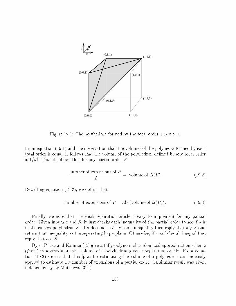
(0,0,0)
(0,0,1)
(0,1,1)
(0,1,0)
(1,0,0)
(1,1,0)
(1,1,1)
(1,0,1)
xyz
Figure 19.1: The polyhedron formed by the total order z > y > x.
From equation (19.1) and the observation that the volumes of the polyhedra formed by eachtotal order is equal, it follows that the volume of the polyhedron de�ned by any total orderis 1=n!. Thus it follows that for any partial order P
number of extensions of P
n!= volume of �(P ): (19:2)
Rewriting equation (19.2), we obtain that
number of extensions of P = n! � (volume of �(P )) : (19:3)
Finally, we note that the weak separation oracle is easy to implement for any partial
order. Given inputs a and S, it just checks each inequality of the partial order to see if a isin the convex polyhedron S. If a does not satisfy some inequality then reply that a 62 S and
return that inequality as the separating hyperplane. Otherwise, if a satis�es all inequalities,reply that a 2 S.
Dyer, Frieze and Kannan [13] give a fully-polynomial randomized approximation scheme
(fpras) to approximate the volume of a polyhedron given a separation oracle. From equa-
tion (19.3) we see that this fpras for estimating the volume of a polyhedron can be easilyapplied to estimate the number of extensions of a partial order. (A similar result was given
independently by Matthews [31].)
153
19.2 Learning a Total Order
In this section we show how to use a fpras to implement a randomized version of the ap-
proximate halving algorithm, and apply this result for the problem of learning a total order
on a set of n elements.
We �rst prove an (n lg n) lower bound on the number of mistakes made by any learning
algorithm. We use the following result of Kahn and Saks [24]: Given any partial order P
that is not a total order there exists an incomparable pair of elements xi,xj such that
3
11�
number of extensions of P with xi � xjnumber of extensions of P
�8
11:
So the adversary can always pick a pair of elements so that regardless of the learner's pre-
diction, the adversary can force a mistake while only eliminating a constant fraction of the
remaining total orders.Finally, we present a polynomial prediction algorithm making n lg n+ (lg e) lg n mistakes
with very high probability. We �rst show how to use an exact counting algorithm R, for
counting the number of concepts in Cn consistent with a given set of examples, to implementthe halving algorithm.
Lemma 19.1 Given a polynomial-time algorithm R to exactly count the number of concepts
in C consistent with a given set E of examples, one can e�ciently implement the halvingalgorithm for C.
Proof: We show how to use R to e�ciently make the predictions required by the halving
algorithm. To make a prediction for an instance x in Xn the following procedure is used:Construct E� fromE by appending x as a negative example to E. Use the counting algorithmR to count the number of concepts C� 2 V that are consistent with E�. Next construct E+
from E by appending x as a positive example to E. As before, use R to count the numberof concepts C+ 2 V that are consistent with E+. Finally if jC�j � jC+j then predict that x
is a negative example; otherwise predict that x is a positive example.
Clearly a prediction is made in polynomial time, since it just requires calling R twice. Itis also clear that each prediction is made according to the majority of concepts in V.
We modify this basic technique to use a fpras instead of the exact counting algorithmto obtain an e�cient implementation of a randomized version of the approximate halving
algorithm.
Theorem 19.2 Let R be a fpras for counting the number of concepts in Cn consistent witha given set E of examples. If jXnj is polynomial in n, one can produce a prediction algorithm
that for any � > 0 runs in time polynomial in n and lg 1�and makes at most lg jCnj
�1 + lg e
n
�mistakes with probability at least 1� �.
Proof: The prediction algorithm implements the procedure described in Lemma 19.1 with
the exact counting algorithm replaced by the fpras R(n; 1n; �2jXnj
). Consider the prediction
154
for an instance x 2 Xn. Let V be the set of concepts that are consistent with all previous
instances. Let r+ (respectively r�) be the number of concepts in V for which x is a positive
(negative) instance. Let r+ (respectively r�) be the estimate output by R for r+ (r�). Since
R is a fpras, with probability at least 1� �jXnj
r�
1 + �� r� � (1 + �)r� and
r+
1 + �� r+ � (1 + �)r+
where � = 1=n. Without loss of generality, assume that the algorithm predicts that x is a
negative instance, and thus r� � r+. Combining the above inequalities and the observation
that r� + r+ = jVj, we obtain that r� � jVj
1+(1+�)2.
We de�ne an appropriate prediction to be a prediction that agrees with at least jVj
1+(1+�)2
of the concepts in V. To analyze the mistake bound for this algorithm, suppose that each
prediction is appropriate. For a single prediction to be appropriate, both calls to the fpras Rmust output a count that is within a factor of 1+� of the true count. So any given predictionis appropriate with probability at least 1� �
jXnj, and thus the probability that all predictions
are appropriate is at least
1 � jXnj
�
jXnj
!= 1 � �:
Clearly if all predictions are appropriate then the above procedure is in fact an implemen-
tation of the approximate halving algorithm with ' = 11+(1+�)2
and thus by Theorem 19.1 at
most log(1�')�1 jCnj mistakes are made. Substituting � with its value of 1n
and simplifyingthe expression we obtain that with probability at least 1 � �,
# mistakes �lg jCnj
lg 11�'
=lg jCnj
lg�1 + n2
n2+2n+1
� : (19:4)
Since n2
n2+2n+1� 1� 2
n,
1
lg�1 + n2
n2+2n+1
� �1
lg�1 + 1 � 2
n
�
=1
1 + lg�1 � 1
n
�
= 1 �lg�1 � 1
n
�1 + lg
�1 � 1
n
�
We now derive two inequalities which we use to �nish up the analysis. Since for all x,ex � 1 + x, by letting x = �1=n, taking logarithms of both sides and then adding 1 to each
side, we obtain that
1 + lg
�1 �
1
n
�� 1 �
lg e
n:
155
Next be letting x = 1=(n � 1) in ex � 1 + x and raising both sides to the power of n� 1 we
get that:
e ��
1 +1
n� 1
�n�1=
�n
n� 1
�n�1:
Taking the logarithm of both sides and simplifying yields that
lg
�1�
1
n
��� lg e
n � 1:
We now apply the inequalities lg�1� 1
n
�� � lg e
n�1and 1 + lg
�1 � 1
n
�� 1� lg e
nto get that
lg�1 � 1
n
�1 + lg
�1� 1
n
� �� lg en�1
1� lg en
=� lg e
n� 1� n�1n
lg e
�� lg e
n
Finally, applying these inequalities to equation (19.4) yields that
# mistakes �lg jCnj
lg�1 + n2
n2+2n+1
� � lg jCnj
1 +
lg e
n
!:
Note that we could modify the above proof by not requiring that all predictions beappropriate. In particular if we allow predictions not to be appropriate then we get amistake bound of lg jCnj
�1 + lg e
n
�+ .
We now apply this result to obtain the main result of this section. Namely, we describea randomized polynomial prediction algorithm for learning a total order in the case that the
adversary selects the query sequence.
Theorem 19.3 There exists a prediction algorithm A for learning total orders such that oninput � (for all � > 0), and for any query sequence provided by the adversary, A runs in
time polynomial in n and lg 1�and makes at most n lg n+ (lg e) lg n mistakes with probability
at least 1 � �.
Proof Sketch: We apply the results of Theorem 19.2 using the fpras for counting the number
of extensions of a partial order given independently by Dyer, Frieze and Kannan [13], andby Matthews [31]. We know that with probability at least 1 � �, the number of mistakes is
at most lg jCnj�1 + lg e
n
�. Since jCnj = n! the desired result is obtained.
We note that the probability that A makes more than n lg n + (lg e) lg n mistakes does
not depend on the query sequence selected by the adversary. The probability is taken over
the coin ips of the randomized approximation scheme.
156
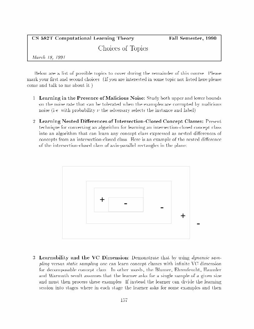
CS 582T Computational Learning Theory Fall Semester, 1990
Choices of TopicsMarch 18, 1991
Below are a list of possible topics to cover during the remainder of this course. Please
mark your �rst and second choices. (If you are interested in some topic not listed here please
come and talk to me about it.)
1. Learning in the Presence of Malicious Noise: Study both upper and lower bounds
on the noise rate that can be tolerated when the examples are corrupted by malicious
noise (i.e. with probability � the adversary selects the instance and label).
2. Learning Nested Di�erences of Intersection-Closed Concept Classes: Presenttechnique for converting an algorithm for learning an intersection-closed concept class
into an algorithm that can learn any concept class expressed as nested di�erences ofconcepts from an intersection-closed class. Here is an example of the nested di�erenceof the intersection-closed class of axis-parallel rectangles in the plane:
+
-+
- -
3. Learnability and the VC Dimension: Demonstrate that by using dynamic sam-
pling versus static sampling one can learn concept classes with in�nite VC dimensionfor decomposable concept class. In other words, the Blumer, Ehrenfeucht, Haussler
and Warmuth result assumes that the learner asks for a single sample of a given size
and must then process these examples. If instead the learner can divide the learningsession into stages where in each stage the learner asks for some examples and then
157
performs some processing, then it is possible to learn any concept class that can be
written as the countable union
C = C1 [ C2 [ � � �
where each concept class Cd has VC dimension at most d.
4. On the Sample Complexity of Weak Learning: Study the sample complex-
ity needed to weakly learn. Although Schapire has shown that any concept weakly
learnable is also strongly learnable, his work does not address the number of examples
needed to weakly learn. It is shown to be important to distinguish between those learn-
ing algorithms that output deterministic hypothesis and those that output randomized
hypothesis.
5. Learning DFA With Membership and Equivalence Queries: Present an al-
gorithm that can learn any DFA with membership and equivalence queries in timepolynomial in the number of states in the minimum DFA and the length of the longestcounterexample.
6. Learning Read-Once Formulas with Membership and Equivalence Queries:Present an algorithm that can learn any read-once formula in time polynomial in the
number of variables and the length of the formula. Also an algorithm to learn anymonotone read-once formula using only membership queries is presented.
7. Separating the PAC and Mistake-Bound Model over the Boolean Domain:Over the domain f0; 1gn it is known that if the learner is allowed unlimited computa-tional resources then any concept class learning in one of these two models is learnable
in the other. In addition, any polynomial-time learning algorithm for a concept classin the mistake-bound model can be transformed into one that learns the class in thePAC model. Here it is shown that if one-way functions exists then the converse doesnot hold. Namely, a concept class over f0; 1gn is given that is not learnable in themistake-bound model but is learnable in the PAC model. Furthermore, the concept
class remains hard to learn in the mistake-bound model even if the learner is allowed
a polynomial number of membership queries.
8. Using Approximate Counting Schemes to E�ciently Implement a Random-
ized Version of the Halving Algorithm: Study a technique to e�ciently implementthe halving algorithm given an appropriate approximate counting scheme. In partic-
ular, it is shown how a scheme to approximate the number of extensions of a partial
order can be used to learn the concept class of total orders under the mistake boundmodel (with adversary presentation) making only O(n lg n) mistakes.
9. The Weighted Majority Algorithm: Study construction of a prediction algorithm
in a situation in which a learner faces a sequence of trials, with a prediction to be made
in each, and the goal of the learner is to make few mistakes. In particular, consider
158
the case in which the learner has reason to believe that one of some pool of known
algorithms will perform well, but the learner does not know which one. A simple and
e�ective method, based on weighted voting, is introduced for constructing a compound
algorithm in such a circumstance. This algorithm is shown to be robust with respect
to errors in the data.
10. Learning Boolean Functions in an In�nite Attribute Space: Consider a model
for learning Boolean functions in domains described by a potentially in�nite number
of attributes. (The learner is just shown the attributes which are true and must run in
time polynomial in the number of attributes revealed.) It is shown that many of the
basic Boolean functions learnable in the standard model such as k-CNF and k-DNF
are still learnable in the new model, though by more complicated algorithms.
11. Training a 3-Node Neural Network is NP-Complete: It is shown that given asimple 2-layer 3-node, n-input neural network whose nodes compute linear thresholdfunctions of their inputs, that it is NP-complete to decide whether there exist linear
threshold functions for the three nodes of this network so that it will produce outputconsistent with a given set of training examples. The proof involves translating thelearning problem into a geometrical setting. An equivalent statement of the result isthat it is NP-complete to decide whether two sets of Boolean vectors in n-dimensionalspace can be separated by two hyperplanes so that some quadrant contains all theelements of one set and none of the other.
12. Inferring Graphs from Walks: Consider the problem of inferring an undirected,degree-bounded, edge-colored graph from the sequence of edge colors seen in a walk of
that graph. This problem can be viewed as reconstructing the structure of a Markovchain from its output. A polynomial-time algorithm for the inference of underlyinggraphs of degree-bound 2 is presented.
159

160
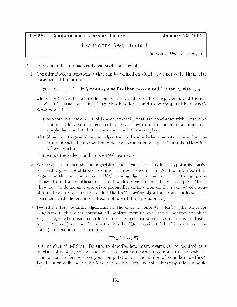
CS 582T Computational Learning Theory January 25, 1991
Homework Assignment 1Solutions Due: February 8
Please write up all solutions clearly, concisely, and legibly.
1. Consider Boolean functions f that can by de�ned on f0; 1gn by a nested if{then{else
statement of the form:
f(x1; x2; . . . ; xn) = if l1 then c1 elseif l2 then c2 � � � elseif lk then ck else ck+1
where the lj's are literals (either one of the variables or their negations), and the cj's
are either T (true) or F (false). (Such a function is said to be computed by a simpledecision list .)
(a) Suppose you have a set of labeled examples that are consistent with a functioncomputed by a simple decision list. Show how to �nd in polynomial time somesimple decision list that is consistent with the examples.
(b) Show how to generalize your algorithm to handle k-decision lists, where the con-dition in each if statement may be the conjunction of up to k literals. (Here k isa �xed constant.)
(c) Argue the k-decision lists are PAC learnable.
2. We have seen in class that an algorithm that is capable of �nding a hypothesis consis-tent with a given set of labeled examples can be turned into a PAC learning algorithm.Argue that the converse is true: a PAC learning algorithm can be used (with high prob-ability) to �nd a hypothesis consistent with a given set of labeled examples. (Hint:Show how to de�ne an appropriate probability distribution on the given set of exam-
ples, and how to set � and �, so that the PAC learning algorithm returns a hypothesisconsistent with the given set of examples, with high probability.)
3. Describe a PAC learning algorithm for the class of concepts k-RS(n) (the RS is for\ring-sum"); this class contains all boolean formula over the n boolean variables
fx1; . . . ; xng, where each such formula is the exclusive-or of a set of terms, and eachterm is the conjunction of at most k literals. (Once again, think of k as a �xed con-
stant.) For example, the formula
x1x3x5 � x2 � x4
is a member of 3-RS(5). Be sure to describe how many examples are required as a
function of n, k, �, and �, and how the learning algorithm computes its hypothesis.
(Hints: For the former, base your computation on the number of formula in k-RS(n).For the later, de�ne a variable for each possible term, and solve linear equations modulo
2.)
161
4. Consider the class of concepts de�ned on the interval on the interval (0; 1) where each
concept is of the form (0; r] for some real r 2 (0; 1). For the concept (0; r], all real
numbers x, 0 < x � r, are positive instances while all real numbers y, r < y < 1, are
negative instances. There is one such concept for each real number r 2 f0; 1g.
(a) Show that this concept class is PAC learnable under the assumption that the ex-
amples are drawn uniformly from the range (0; 1). Specify the number of examples
needed as a function of � and �, and explain how you construct your hypothesis
from the given data.
(b) Show that this concept class is PAC learnable when the examples are drawn
according to some unknown distribution. Specify the number of examples needed
as a function of � and �, and explain how you construct your hypothesis from the
given data.
5. Let y be a Bernoulli random variable that is 1 with probability p. Our goal is tocompute a good estimate for p from observing a set of independent draws of y. Let pbe an estimate of p obtained from m independent trials. That is p is just:
(number of trials in which y = 1) / (total number of trials)
How large must m be so that Pr[jp� pj � ] � �. That is we want our estimate for pto be within of the true value for p with probability at least 1� �.
162
CS 582T Computational Learning Theory February 20, 1991
Homework Assignment 2Solutions Due: March 6
Please write up all solutions clearly, concisely, and legibly.
1. We return to the class of concepts de�ned on the interval (0; 1) where each concept is
of the form (0; r] for some real r 2 (0; 1). Suppose that the source of labeled examples
is subject to random misclassi�cation noise of a rate � < 1=4. Give a PAC learning
algorithm for this problem. Be sure to specify how many examples are needed as a
function of � and � (and � if you wish).
2. If C1 and C2 are concept classes, and c1 2 C1 and c2 2 C2, then c1 _ c2 is the concept
whose positive examples are exactly the set c1 [ c2. Note that c1 _ c2 may not be anelement of either C1 or C2. We can then de�ne the concept class C1 _ C2 = fc1 _ c2 :c1 2 C1; c2 2 C2g. The de�nition for the class C1 ^ C2 is analogous.
(a) Prove that if C1 is PAC learnable, and C2 is PAC learnable from negative exam-ples, then C1 _ C2 is PAC learnable.
(b) Prove that if C1 is PAC learnable from positive examples and C2 is PAC learnablefrom positive examples then C1 ^ C2 is PAC learnable from positive examples.
3. Let C, C1, C2 be concept classes of �nite VC-dimension over instance space X.
(a) De�ne C = fX � c : c 2 Cg. What is V CD(C) in terms of V CD(C)?
(b) For concept class C, let V CD(C) = d and let S be any set of m distinct instances.
Prove that j�C(S)j � �d(m) =Pd
i=0
�m
i
�. (Recall that �C(S) includes all distinct
ways that C can classify the S instances.)
Hint: Use induction on m and d. (Think about m = d as the base case for anygiven d.) Also, it may be useful to show that �d(m) = �d(m� 1) + �d�1(m� 1).
(c) For concept classes C1, C2, prove that V CD(C1[C2) � V CD(C1)+V CD(C2)+1.
Also provide an example to demonstrate that this result is the best possible suchresult.
4. Show how to exactly identify any unknown read-once-DNF formula using a polyno-
mial number of equivalence and membership queries. In a read-once formula each
variable occurs at most once. (The one instance of a variable may be either negated
or unnegated|so a read-once formula need not be a monotone formula.) The numberof queries should be polynomial in the number of terms and variables in the unknown
formula.
163
Big Hint: Prove as a lemma that if f is the unknown read-once-DNF formula over the
variables X1; . . . ;Xn, and x = (x1; . . . ; xn) and y = (y1; . . . ; yn) are two assignments to
these variables such that x and y agree in all but one variable assignment, yet f(x) = 1
and f(y) = 0, then S(x) is a term of f , where S(x) is the conjunction of the literals in
the set
fXi : f(x� i) = 0 and xi = 1g [nXi : f(x� i) = 0 and xi = 0
o
where x�i is the assignment x with the ith variable ipped. (For example 00110�3 =
00010.)
extra credit:
Let C be a concept class of �nite VC-dimension over instance space X. Let
C(k) = f[ki=1ci : ci 2 Cg:
Prove that V CD(C(k)) = O(k ln(k) �V CD(C)). (Note the same result holds for k-wayintersection.)
164
CS 582T Computational Learning Theory March 27, 1991
Homework Assignment 3Solutions Due: April 9
Please write up all solutions clearly, concisely, and legibly.
1. Suppose that f1; f2; . . . is an enumeration of some set of computable total 0-1-valued
functions. More precisely, this enumeration is computed by some program M ; the
output of M on input i is a program Pi that computes fi.
Show how to learn an unknown function f , which is guaranteed to be one of the fi's,
in the mistake-bound model described in the Littlestone paper in such a way that you
make only O(lg t) mistakes, where t is the least index such that f = ft.
2. In this problem we considered a simple case of learning with queries where the feedback
can be erroneous. The learner and adversary agree on a number n, and then theadversary thinks of a number between 1 and n, inclusive. The learner must �nd outwhich number the adversary has selected by asking questions of the form, \Is yournumber less than t?" for various t. A binary-search approach allows you to ask atmost lg n questions before �nding the number.
To make this an interesting problem, suppose that the adversary is allowed to incor-rectly respond to at most one question. How many questions must the learner nowask? (A bound of 3 lg n is easy: the learner can just ask each question three times and
take the majority vote of the adversary's responses.) Give a learning algorithm thatuses a number of queries of the form lg n+ f(n) where f(n) = o(lg n), that is, f growsasymptotically more slowly than the logarithm function.
3. Argue that functions representable as 1-decision lists are threshold functions. That is,given any 1-decision list f(x1; x2; . . . ; xn) = if l1 then c1 elseif l2 then c2 � � � elseiflk then ck else ck+1, show how to construct a threshold function equivalent to thisdecision list. One way to achieve this goal is to do the following:
(a) Show that, without loss of generality, you can assume that ck = 1 and ck+1 = 0.
(b) Suppose that the threshold circuit not only has access to the xi for all i, but alsohas access to the negated variables xi for all i. (We will remove this additional in-
formation in the next step.) Given this assumption, describe a threshold functionequivalent to f .
(c) Now modify the previous part so that the threshold function does not have accessto the negated variables.
Observe that now we can use Littlestone's Winnow2 combined with the transformationdescribed in Example 6 from Littlestone's paper (pg. 312) to learn 1-decision lists in
the mistake-bound model.
165
4. In this problem we consider r-of-k threshold functions. (Recall that for this concept
class, X = f0; 1gn. For a chosen set of k (k � n) relevant variables and a given number
r (1 � r � k), an r-of-k threshold function is 1 if and only if at least r of the k relevant
variables are 1.
Assuming that both r and k are unknown to the learner, show that the class of r-
of-k threshold functions can be learned in the mistake-bound model using the halving
algorithm. What mistake bound do you obtain? How does this compare to the mistake
bound obtained by Winnow2? (That is, does one algorithm always perform better than
the other algorithm? If not, state under what conditions each algorithm is best.)
166
Bibliography
[1] Dana Angluin. Learning k-term DNF formulas using queries and counterexamples. Tech-
nical Report YALEU/DCS/RR-559, Yale University Department of Computer Science,
1987.
[2] Dana Angluin. Learning regular sets from queries and counterexamples. Informationand Computation, 75:87{106, November 1987.
[3] Dana Angluin. Queries and concept learning. Machine Learning, 2(4):319{342, 1988.
[4] Dana Angluin. Equivalence queries and approximate �ngerprints. In Proceedings of theSecond Annual Workshop on Computational Learning Theory, pages 134{145, August1989.
[5] Dana Angluin, Michael Frazier, and Leonard Pitt. Learning conjunctions of horn clauses.In Proceedings of the Thirty First Annual Symposium on Foundations of ComputerScience, pages 186{192, October 1990.
[6] Dana Angluin, Lisa Hellerstein, and Marek Karpinski. Learning read-once formulaswith queries. Technical Report UCB/CSD 89/528, University of California BerkeleyComputer Science Division, 1989.
[7] Dana Angluin and Philip Laird. Learning from noisy examples. Machine Learning,2(4):343{370, 1988.
[8] Dana Angluin and Leslie G. Valiant. Fast probabilistic algorithms for hamiltonian
circuits and matchings. Journal of Computer and System Sciences, 18(2):155{193, April1979.
[9] Javed A. Aslam and Ronald L. Rivest. Inferring graphs from walks. In Proceedings ofthe Third Annual Workshop on Computational Learning Theory, pages 359{370, 1990.
[10] Avrim Blum. Learning boolean functions in an in�nite attribute space. In Proceedings
of the Twenty Second Annual ACM Symposium on Theory of Computing, pages 64{72,May 1990.
[11] Anselm Blumer, Andrzej Ehrenfeucht, David Haussler, and Manfred K. Warmuth. Oc-
cam's razor. Information Processing Letters, 24:377{380, April 1987.
167
[12] Anselm Blumer, Andrzej Ehrenfeucht, David Haussler, and Manfred K. Warmuth.
Learnability and the Vapnik-Chervonenkis dimension. Journal of the Association for
Computing Machinery, 36(4):929{965, October 1989.
[13] M. Dyer, A. Frieze, and R. Kannan. A random polynomial time algorithm for estimating
the volumes of convex bodies. In Proceedings of the 21st Annual ACM Symposium on
Theory of Computing, pages 375{381, May 1989.
[14] Michael R. Garey and David S. Johnson. Computers and Intractability: A Guide to the
Theory of NP-Completeness. W. H. Freeman, San Francisco, 1979.
[15] E. Mark Gold. Complexity of automaton identi�cation from given data. Information
and Control, 37:302{320, 1978.
[16] Sally A. Goldman, Ronald L. Rivest, and Robert E. Schapire. Learning binary relations
and total orders. In Proceedings of the Thirtieth Annual Symposium on Foundations ofComputer Science, pages 46{51, October 1989.
[17] Sally A. Goldman and Robert H. Sloan. The di�culty of random attribute noise. Tech-nical Report WUCS{91{29, Washington University, Department of Computer Science,
June 1991.
[18] Sally Ann Goldman. Learning Binary Relations, Total Orders, and Read-once Formulas.PhD thesis, MIT Dept. of Electrical Engineering and Computer Science, July 1990.
[19] Oded Goldreich, Sha� Goldwasser, and Silvio Micali. How to construct random func-
tions. Journal of the ACM, 33(4):792{807, 1986.
[20] G.H. Hardy, J.E. Littlewood, and G. P�olya. Inequalities. Cambridge University Press,Cambridge, 1959.
[21] David Haussler, Michael Kearns, Nick Littlestone, and Manfred K. Warmuth. Equiva-lence of models for polynomial learnability. Information and Computation. To appear. Apreliminary version is available in Proceedings of the 1988 Workshop on Computational
Learning Theory, pages 42{55, 1988.
[22] Wassily Hoe�ding. Probability inequalities for sums of bounded random variables. Jour-
nal of the American Statistical Association, 58(301):13{30, March 1963.
[23] G�erard Huet. Con uent reductions: Abstract properties and applications to term rewrit-ting systems. In Proceedings of the 18th Annual Symposium on Foundations of Computer
Science, pages 30{45, 1977.
[24] Je� Kahn and Michael Saks. Balancing poset extensions. Order 1, pages 113{126, 1984.
[25] Michael Kearns and Ming Li. Learning in the presence of malicious errors. In Proceedings
of the Twentieth Annual ACM Symposium on Theory of Computing, May 1988.
168
[26] Michael Kearns and Leslie Valiant. Cryptographic limitations on learning Boolean for-
mulae and �nite automata. In Proceedings of the Twenty-First Annual ACM Symposium
on Theory of Computing, pages 433{444, May 1989.
[27] Michael J. Kearns. The Computational Complexity of Machine Learning. MIT Press,
Cambridge, Massachusetts, 1990.
[28] Nathan Linial, Yishay Mansour, and Ronald L. Rivest. Results on learnability and the
Vapnik-Chervonenkis dimension. In Proceedings of the Twenty-Ninth Annual Sympo-
sium on Foundations of Computer Science, pages 120{129, October 1988.
[29] Nick Littlestone. Learning when irrelevant attributes abound: A new linear-threshold
algorithm. Machine Learning, 2:285{318, 1988.
[30] Nick Littlestone and Manfred K. Warmuth. The weighted majority algorithm. In
Proceedings of the Thirtieth Annual Symposium on Foundations of Computer Science,pages 256{261, October 1989.
[31] Peter Matthews. Generating a random linear extension of a partial order. Unpublishedmanuscript, 1989.
[32] D.S. Mitrinovi�c. Analytic Inequalities. Springer-Verlag, New York, 1970.
[33] Leonard Pitt and Leslie G. Valiant. Computational limitations on learning from exam-ples. Journal of the Association for Computing Machinery, 35(4):965{984, 1988.
[34] Leonard Pitt and Manfred Warmuth. Reductions among prediction problems: On thedi�culty of predicting automata (extended abstract). In 3rd IEEE Conference on Struc-ture in Complexity Theory, pages 60{69, June 1988.
[35] Ronald L. Rivest. Learning decision lists. Machine Learning, 2(3):229{246, 1987.
[36] Ronald L. Rivest and Robert E. Schapire. Inference of �nite automata using homingsequences. In Proceedings of the Twenty-First Annual ACM Symposium on Theory ofComputing, pages 411{420, May 1989.
[37] Robert E. Schapire. The strength of weak learnability. Machine Learning, 1990. Special
issue for COLT 89, to appear. A preliminary version is available in Proceedings of the
Thirtieth Annual Symposium on Foundations of Computer Science, pages 28{33,1989.
[38] George Shackelford and Dennis Volper. Learning k-DNF with noise in the attributes.In First Workshop on Computatinal Learning Theory, pages 97{103, Cambridge, Mass.
August 1988. Morgan Kaufmann.
[39] Alistair Sinclair. Randomised Algorithms for Counting and Generating Combinatorial
Structures. PhD thesis, University of Edinburgh, Department of Computer Science,November 1988.
169
[40] Robert H. Sloan. Some notes on Cherno� bounds. (Unpublished), 1987.
[41] Robert H. Sloan. Types of noise in data for concept learning. In First Workshop on
Computational Learning Theory, pages 91{96. Morgan Kaufmann, 1988.
[42] Leslie Valiant. The complexity of computing the permanent. Theoretical Computer
Science, 8:198{201, 1979.
[43] Leslie Valiant. A theory of the learnable. Communications of the ACM, 27(11):1134{
1142, November 1984.
[44] Leslie Valiant. Learning disjunctions of conjunctions. In Proceedings of Ninth Interna-
tional Joint Conference on Arti�cial Intelleigence, 1985.
170