linear difference equations - weill cornell...

Quantitative Understanding in Biology Module III: Linear Difference Equations Lecture I: Introduction to Linear Difference Equations

Introductory Remarks This section of the course introduces dynamic systems; i.e., those that evolve over time. Although

dynamic systems are typically modeled using differential equations, there are other means of modeling

them. While we will spend a good deal of time working with differential equations in the next section,

we’ll begin by considering a close cousin of the differential equation: the difference equation. We will

note here that when we solve differential equations numerically using a computer, we often really solve

their difference equation counterparts. So having some facility with difference equations is important

even if you think of your dynamic models in terms of differential equations.

We’ll also spend some time in this section talking about techniques for developing and expressing

models. While there is often more art than science involved, there are some good practices that we will

share.

This section of the course will also begin to emphasize matrix formulations of models and linear algebra.

We will begin our exploration of these topics with two examples; one from molecular evolution and one

from population dynamics.

An Molecular Evolution Example (Mathematical Models in Biology; Allman and Rhodes)

A fundamental part of molecular evolution is the study of mutations of DNA sequences. As you know, a

DNA molecule is a sequence made up from four nucleic acids: adenine, guanine, cytosine, and thymine.

Adenine and guanine are chemically similar and are called purines; cytosine and thymine are also similar

and are called pyrimidines.

Some simple mutations that a DNA sequence can undergo include deletions, insertions, and single

nucleotide substitutions. DNA can also undergo bulk mutations such as the inversion (reversal) or

duplication of a stretch of DNA. In fact, even entire genome duplications have occurred.

For our current purposes, however, we will consider only single nucleotide substitutions, and focus on

the estimation of mutation rates. Within this family of mutations, substitutions that involve swapping a

Linear Difference Equations

© Copyright 2008, 2012 – J Banfelder, Weill Cornell Medical College

purine with a pyrimidine are called transversions. Transitions are substitutions that leave the class of

nucleotide unchanged.

Consider the ancestral sequence, S0, an intermediate sequence S1, and a descendant S2.

S0: ACCTGCGCTA S1: ACGTGCACTA S2: ACGTGCGCTA

Seeing all three sequences, we count three mutation events. However, if we did not have knowledge of

the intermediate sequence, we would only observe one mutation event, and might naïvely

underestimate the mutation rate. This error arises from the back-mutation at the seventh position in the

sequence. To understand how back-mutations can affect estimates of mutation rates, we’ll build and

explore a simple model of nucleotide substitution.

Imagine that at a single position in the genome we begin with a cytosine nucleotide at time t=0. After

some discrete time period t=1, and there is a probability that the nucleotide will change. In our simplest

model, we will assume that all possible substitutions (transitions and transversions) are equally likely.

We will denote the probability of each possible mutation as α. We then have

P1(A) = α P1(G) = α P1(C) = 1-3α P1(T) = α

Note that our initial condition can also be expressed in terms of probabilities.

P0(A) = 0 P0(G) = 0 P0(C) = 1 P0(T) = 0

After a second time step, our system evolves again. The probability of observing a C at this position is

now

P2(C) = P1(A)∙α + P1(G)∙α + P1(C)∙(1-3α) + P1(T)∙α = 3∙α2 + (1-3α)2

The probability of observing an A at this position is

P2(A) = P1(A)∙(1-3α) + P1(G)∙α + P1(C)∙α + P1(T)∙α = α∙(1-3α) + α∙α + ∙(1-3α)∙α + α∙α =2∙α∙(1-3α) + 2∙α2

The probability for G and T will be same, so we have



P2(A) = 2∙α∙(1-3α) + 2∙α2

P2(G) = 2∙α∙(1-3α) + 2∙α2

P2(C) = 3∙α2 + (1-3α)2

P2(T) = 2∙α∙(1-3α) + 2∙α2

We could carry on this way with t=3, 4, 5… There would be a fair amount of algebra (although we could

probably simplify things along the way). An alternative is to formulate our problem in terms of matrices

and linear algebra. The motivation for doing this is not simply to save on tedium (although that would

probably be reason enough). More importantly, since there is an enormous body of theory already

developed around matrices and linear algebra, if we can cast our problem in this context, we inherit an

enormous body on knowledge and tools for free.

We’ll begin by defining a vector to hold the state variables of our system. The state variables in a model

hold all of the information you need to fully specify the dynamic state of the system. In other words,

anything that might change over time is considered a state variable. For our first pass at this, we would

define our vector of state variables as

(

)

Note that technically we only need three of these values to fully specify the dynamic state of our

system. There is an implied constitutive equation Pi(A) + Pi(G) + Pi(C) + Pi(T) = 1, and a three element

vector would be sufficient. You have probably seen this line of reasoning before in your thermodynamics

classes. You only need to specify two state variables (say, temperature and pressure) of a pure

substance; everything else (enthalpy, density, etc.) can be computed from the equations of state for

that substance. Admittedly, those equations are a good deal more complex, but the idea is the same.

We’ll have more to say about this concept later.

We can also define a state transition matrix, M, as

(

)

The system under investigation then works out quite cleanly. We can write…

si+1 = M∙si

…or, even more generally…

sn = Mn∙s0



A quick review of matrix multiplication In the above discussion, we made use of some prior knowledge you may have had regarding matrix

multiplication. Here we’ll review…

If you have two matrices, A and B, you can multiply them if the number of columns in A is equal to the

number of rows in B. The resultant product will have the same number of rows as A and the same

number of columns as B. In other words

Am×k ∙ Bk×n = Cm×n

This implies one very important property of matrix multiplication: the order of the terms matters. We

say that matrix multiplication is not commutative. In the above example, B∙A would not necessarily even

be defined. Even if it were (in which case m=n), the product would not necessarily be the same. In fact, if

m=n≠k, then the products would not be the same size. For this reason, you’ll often hear phrases as

‘multiply B on the left by A’.

In general, if we have two compatible matrices Am×k and Bk×n, matrix multiplication is defined as follows:

Cm×n = Am×k ∙ Bk×n

∑

It is helpful to visualize this. Each element in the resultant product matrix C is a sum of products. You

take elements in a row of the first matrix and multiply them by the corresponding elements in a column

of the second matrix. Then sum the products.

(

)

(

)

(

)



While matrix multiplication is not commutative, it is associative. This means that the order of operations

(within a string of multiplications) does not matter. In other words, you can prove (A∙B)∙C = A∙(B∙C). This

implies that we can simply write A∙B∙C, and one can perform the operations in any arbitrary order.

A vector can be thought of as a special case of a matrix that happens to have one column. Often, you’ll

see vectors written lengthwise to save space; for example, we could have written our definition of the

state variable vector like so:

si = ( Pi(A) Pi(G) Pi(C) Pi(T) )

However, for purposes of multiplication, the vector should be thought of as a column vector.

The transpose of a matrix is written as At. All that this means is that we swap rows with columns. So if

Bnxm = (Amxn)t, then bi,j = aj,i. The transpose of a column vector is a row vector, which is just a 1xm matrix.

Example: If v and w are vectors, what are the dimensions of vt ∙ w, and when is it defined?

( )

Note that the vectors need to be the same length for this computation to be defined. The result is a

scalar value. Note that in the case of vectors, we could also just write v∙w, which is the scalar product (or

dot product) of the two vectors. The result is the same.

Example: If v and w are vectors, what are the dimensions of v ∙ wt, and when is it defined?

( ) (

)

Here we get something reminiscent of a multiplication table. Note that the vectors do not need to be

the same length. The table will have as many rows as the length of the first vector, and as many columns

as the length of the second.

Example: Consider a matrix, M, that holds observed (x,y) data from an experiment, augmented with a

column of ones. Compute Mt∙M.

(

)

(

)(

) (

)



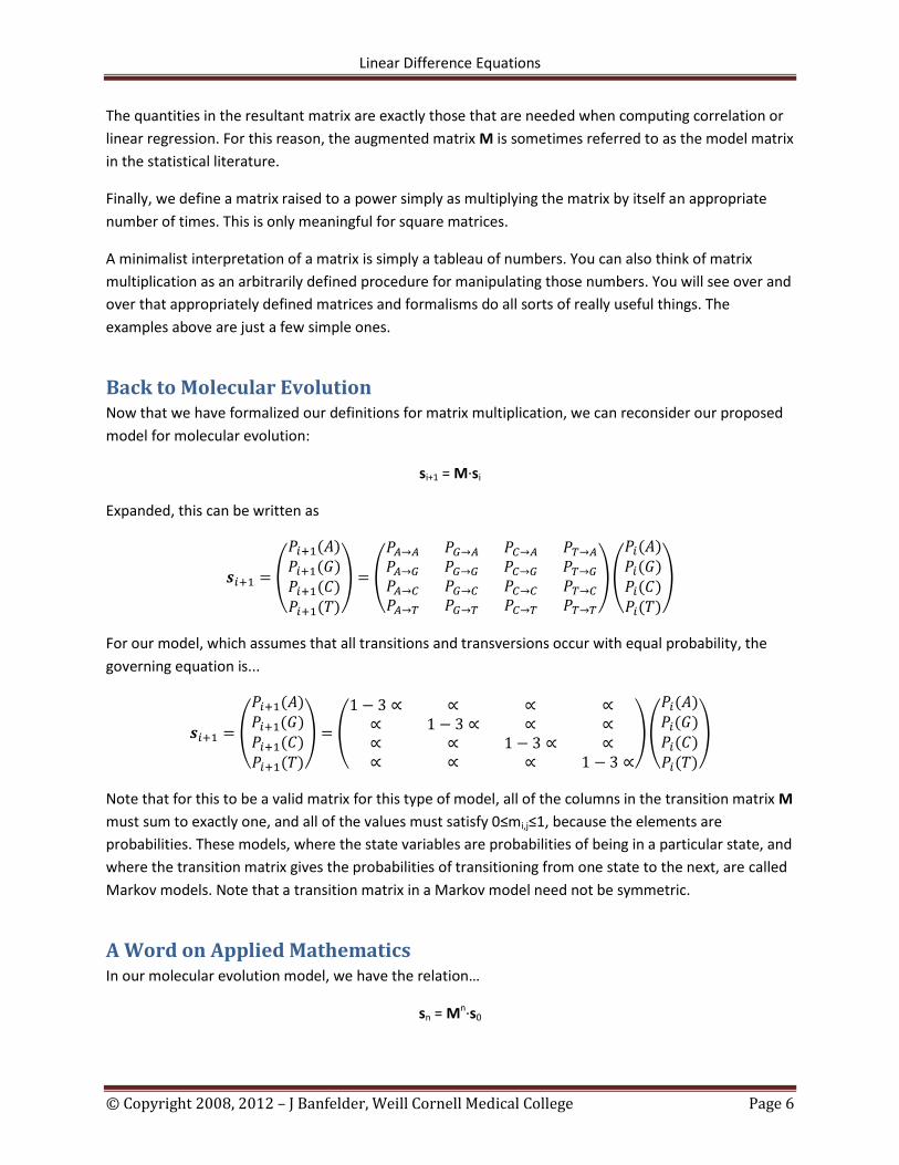
The quantities in the resultant matrix are exactly those that are needed when computing correlation or

linear regression. For this reason, the augmented matrix M is sometimes referred to as the model matrix

in the statistical literature.

Finally, we define a matrix raised to a power simply as multiplying the matrix by itself an appropriate

number of times. This is only meaningful for square matrices.

A minimalist interpretation of a matrix is simply a tableau of numbers. You can also think of matrix

multiplication as an arbitrarily defined procedure for manipulating those numbers. You will see over and

over that appropriately defined matrices and formalisms do all sorts of really useful things. The

examples above are just a few simple ones.

Back to Molecular Evolution Now that we have formalized our definitions for matrix multiplication, we can reconsider our proposed

model for molecular evolution:

si+1 = M∙si

Expanded, this can be written as

(

) (

)(

)

For our model, which assumes that all transitions and transversions occur with equal probability, the

governing equation is...

(

) (

)(

)

Note that for this to be a valid matrix for this type of model, all of the columns in the transition matrix M

must sum to exactly one, and all of the values must satisfy 0≤mi,j≤1, because the elements are

probabilities. These models, where the state variables are probabilities of being in a particular state, and

where the transition matrix gives the probabilities of transitioning from one state to the next, are called

Markov models. Note that a transition matrix in a Markov model need not be symmetric.

A Word on Applied Mathematics In our molecular evolution model, we have the relation…

sn = Mn∙s0



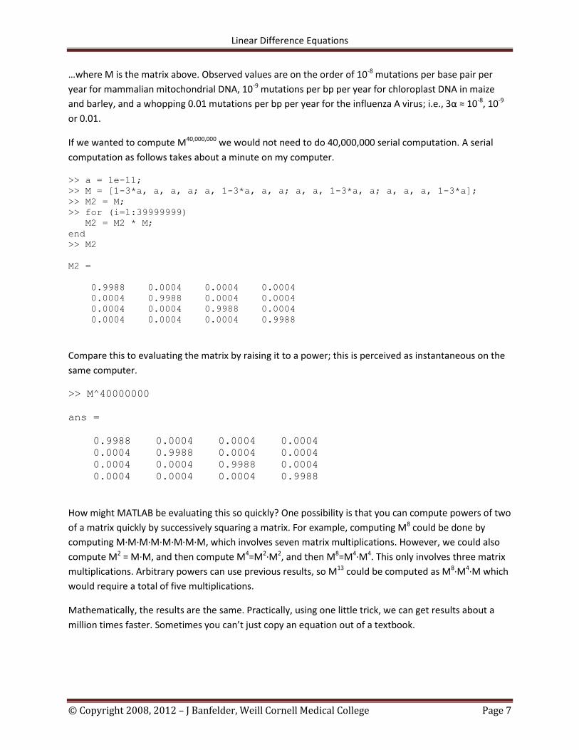
…where M is the matrix above. Observed values are on the order of 10-8 mutations per base pair per

year for mammalian mitochondrial DNA, 10-9 mutations per bp per year for chloroplast DNA in maize

and barley, and a whopping 0.01 mutations per bp per year for the influenza A virus; i.e., 3α ≈ 10-8, 10-9

or 0.01.

If we wanted to compute M40,000,000 we would not need to do 40,000,000 serial computation. A serial

computation as follows takes about a minute on my computer.

>> a = 1e-11;

>> M = [1-3*a, a, a, a; a, 1-3*a, a, a; a, a, 1-3*a, a; a, a, a, 1-3*a];

>> M2 = M;

>> for (i=1:39999999)

M2 = M2 * M;

end

>> M2

M2 =

0.9988 0.0004 0.0004 0.0004

0.0004 0.9988 0.0004 0.0004

0.0004 0.0004 0.9988 0.0004

0.0004 0.0004 0.0004 0.9988

Compare this to evaluating the matrix by raising it to a power; this is perceived as instantaneous on the

same computer.

>> M^40000000

ans =

0.9988 0.0004 0.0004 0.0004

0.0004 0.9988 0.0004 0.0004

0.0004 0.0004 0.9988 0.0004

0.0004 0.0004 0.0004 0.9988

How might MATLAB be evaluating this so quickly? One possibility is that you can compute powers of two

of a matrix quickly by successively squaring a matrix. For example, computing M8 could be done by

computing M∙M∙M∙M∙M∙M∙M∙M, which involves seven matrix multiplications. However, we could also

compute M2 = M∙M, and then compute M4=M2∙M2, and then M8=M4∙M4. This only involves three matrix

multiplications. Arbitrary powers can use previous results, so M13 could be computed as M8∙M4∙M which

would require a total of five multiplications.

Mathematically, the results are the same. Practically, using one little trick, we can get results about a

million times faster. Sometimes you can’t just copy an equation out of a textbook.



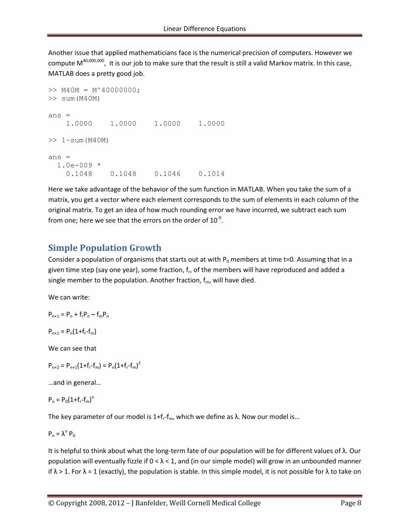
Another issue that applied mathematicians face is the numerical precision of computers. However we

compute M40,000,000, it is our job to make sure that the result is still a valid Markov matrix. In this case,

MATLAB does a pretty good job.

>> M40M = M^40000000;

>> sum(M40M)

ans =

1.0000 1.0000 1.0000 1.0000

>> 1-sum(M40M)

ans =

1.0e-009 *

0.1048 0.1048 0.1046 0.1014

Here we take advantage of the behavior of the sum function in MATLAB. When you take the sum of a

matrix, you get a vector where each element corresponds to the sum of elements in each column of the

original matrix. To get an idea of how much rounding error we have incurred, we subtract each sum

from one; here we see that the errors on the order of 10-9.

Simple Population Growth Consider a population of organisms that starts out at with P0 members at time t=0. Assuming that in a

given time step (say one year), some fraction, fr, of the members will have reproduced and added a

single member to the population. Another fraction, fm, will have died.

We can write:

Pn+1 = Pn + frPn – fmPn

Pn+1 = Pn(1+fr-fm)

We can see that

Pn+2 = Pn+1(1+fr-fm) = Pn(1+fr-fm)2

…and in general…

Pn = P0(1+fr-fm)n

The key parameter of our model is 1+fr-fm, which we define as λ. Now our model is…

Pn = λn P0

It is helpful to think about what the long-term fate of our population will be for different values of λ. Our

population will eventually fizzle if 0 < λ < 1, and (in our simple model) will grow in an unbounded manner

if λ > 1. For λ = 1 (exactly), the population is stable. In this simple model, it is not possible for λ to take on



negative values, since its definition will not admit the possibility. Mathematically, we would expect to

see oscillations between positive and negative population values; oscillations are OK, but a negative

population doesn’t make sense. We’ll get back to this point in a while.

The exponential growth we see here is a critical result, and understanding how this growth behaves for

different values of λ can’t be overemphasized.

(Slightly) More Complex Population Growth (Mathematical Model in Biology, Edelstein-Keshet)

Let us consider a slightly more complex example of population growth. We’ll develop a model for the

population of annual plants.

In our model, annual plants produce γ seeds per plant in the fall of each year. Seeds remain in the

ground for up to two years. Some fraction of one-year-old seeds, α, germinate during the spring. Some

fraction of two-year-old seeds, β, germinate during the spring. All plants die during the winter.

We’ll begin by defining three state variables:

Pn The number of plants that germinate from seeds during year n

S1n The number of one year old seeds in the ground at the beginning of the spring of year n

S2n The number of two-year-old seeds in the ground at the beginning of the spring of year n

It is always a very good idea to write down precise definitions of your model variables.

Our model, translated from words into equations, tells us that

Pn = α∙S1n + β∙S2n S1n+1 = γ∙Pn S2n+1 = (1-α)∙S1n

Since we like to write future variables in terms of present variables, we will write…

Pn+1 = α∙S1n+1 + β∙S2n+1

…and then substitute our ‘definitions’ of S1 and S2…

Pn+1 = α∙γ∙Pn + β∙(1-α)∙S1n

So it turns out that we can track the evolution of our system only by keeping track of P and S1.

Pn+1 = α∙γ∙Pn + β∙(1-α)∙S1n S1n+1 = γ∙Pn We have reduced our model to a system of linear difference equations. This begs for a matrix representation. In fact, we can write…



(

) (

) (

)

We can use this formulation to predict how the model will evolve over time by raising the matrix to any given power. Ideally, it would be nice to be able to treat the system analytically, and see if we can’t learn anything about the trends in behavior of the system, much as we did in the simple growth model.

Introduction to Eigenvalues We would like to formulate a solution of an arbitrary 2x2 system of linear difference equations. Our

arbitrary system is…

xn+1 = a11 ∙ xn + a12 ∙ yn yn+1 = a21 ∙ xn + a22 ∙ yn

We can turn this into a single equation that incorporates two time steps…

xn+2 = a11 ∙ xn+1 + a12 ∙ yn+1

= a11 ∙ xn+1 + a12 ∙ (a21 ∙ xn + a22 ∙ yn)

= a11 ∙ xn+1 + a12 ∙ a21 ∙ xn + a22 ∙ a12 ∙ yn

= a11 ∙ xn+1 + a12 ∙ a21 ∙ xn + a22 ∙ (xn+1 – a11 ∙ xn)

or

xn+2 – (a11 + a22)xn+1 + (a22 ∙ a11 – a12 ∙ a21)xn = 0

We saw that for a 1x1 system, the solution is xn = x0∙λn. We can try this solution in our case here…

x0∙λn+2 – (a11 + a22) x0∙λ

n+1 + (a22 ∙ a11 – a12 ∙ a21) x0∙λn = 0

Cancelling out a factor of x0∙λ, we get…

λ2 – (a11 + a22) λ + (a22 ∙ a11 – a12 ∙ a21) = 0

…which is a quadratic equation. If we define b = (a11 + a22), and c=(a22 ∙ a11 – a12 ∙ a21), we have

√

So there are two possible values for λ. For now, we’ll consider only the case of two distinct real values

for λ. Other cases (repeated and complex roots) will be considered later.

Since our original system of equations is linear, the principle of superposition applies. This means that

any linear combination of solutions to our system will also be a solution to our system. So our general

solution is…

xn = A1 ∙ λ1n + A2 ∙ λ2

n



As this solution is only a guess, you can go back and substitute this result into the original equation and

prove that it works.

Had we chosen to eliminate x instead of y, our solution would have been…

yn = B1 ∙ λ1n + B2 ∙ λ2

n

The A and B constants are different, but the values of the λs are the same. You can see this in the

definitions for b and c; they are symmetric (substitute aij with aji, and you get the same values of b and c,

and thus the same λ).

The values of λ are called the eigenvalues of the matrix. You can learn an incredible amount about the

long-term behavior of the system simply by knowing the eigenvalues and inspecting these equations.

xn = A1 ∙ λ1n + A2 ∙ λ2

n yn = B1 ∙ λ1

n + B2 ∙ λ2n

Firstly, the eigenvalue with the larger absolute value will dominate the long-term behavior of the

system. For arbitrarily large n, the terms with the smaller eigenvalues will be negligible compared to

those with the larger. Some cases arise:

λ > 1 System grows exponentially

λ = 1 System reaches an equilibrium

0 < λ < 1 System decays

-1 < λ < 0 System decays in an oscillatory manner

λ = -1 System reaches a stationary oscillation

λ < -1 System grows exponentially in an oscillatory manner

All of this applies to larger systems as well. A system with four state variables (such as in our molecular

evolution example), will have four eigenvalues. Its long-term behavior will be governed by the largest.

Eigenvalues for large systems (i.e., large matrices) are usually determined by a computer.

Back to Plants and Seeds Back to our plant example, let us suppose that each plant produces 25 seeds. Let us also suppose that

7% of one-year-old seeds germinate, and that 5% of two-year-old seeds germinate. We can compute the

eigenvalues of this system:

>> alpha=0.07; beta=0.05; gamma=25; M = [alpha * gamma, beta*(1-

alpha); gamma, 0]; eig(M)

ans =

2.2636

-0.5136



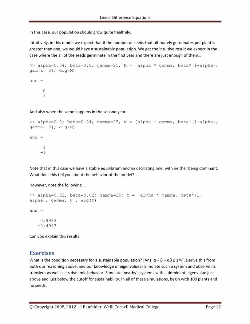
In this case, our population should grow quite healthily.

Intuitively, in this model we expect that if the number of seeds that ultimately germinates per plant is

greater than one, we would have a sustainable population. We get the intuitive result we expect in the

case where the all of the seeds germinate in the first year and there are just enough of them…

>> alpha=0.04; beta=0.0; gamma=25; M = [alpha * gamma, beta*(1-alpha);

gamma, 0]; eig(M)

ans =

0

1

And also when the same happens in the second year…

>> alpha=0.0; beta=0.04; gamma=25; M = [alpha * gamma, beta*(1-alpha);

gamma, 0]; eig(M)

ans =

1

-1

Note that in this case we have a stable equilibrium and an oscillating one, with neither being dominant.

What does this tell you about the behavior of the model?

However, note the following…

>> alpha=0.02; beta=0.02; gamma=25; M = [alpha * gamma, beta*(1-

alpha); gamma, 0]; eig(M)

ans =

0.9933

-0.4933

Can you explain this result?

Exercises What is the condition necessary for a sustainable population? [Ans: α + β – αβ ≥ 1/γ]. Derive this from

both our reasoning above, and our knowledge of eigenvalues? Simulate such a system and observe its

transient as well as its dynamic behavior. Simulate ‘nearby’; systems with a dominant eigenvalue just

above and just below the cutoff for sustainability. In all of these simulations, begin with 100 plants and

no seeds.



>> alpha = 0.02; beta=0.02; gamma=25;

>> M = [alpha * gamma, beta*(1-alpha); gamma, 0];

>> x = [100, 0];

>> for(i=1:30)

x(i+1,:) = M * x(i,:)';

end

>> x

x =

1.0e+003 *

0.1000 0

0.0500 2.5000

0.0740 1.2500

0.0615 1.8500

0.0670 1.5375

0.0636 1.6752

0.0647 1.5910

0.0635 1.6164

0.0634 1.5878

0.0628 1.5859

0.0625 1.5710

0.0620 1.5626

0.0616 1.5511

0.0612 1.5412

0.0608 1.5306

0.0604 1.5205

0.0600 1.5103

0.0596 1.5002

0.0592 1.4901

0.0588 1.4801

0.0584 1.4702

0.0580 1.4604

0.0576 1.4506

0.0572 1.4409

0.0569 1.4312

0.0565 1.4216

0.0561 1.4121

0.0557 1.4027

0.0554 1.3933

0.0550 1.3839

0.0546 1.3747

>> plot(x(:,1))

Other interesting parameter values to plot are

>> alpha=0.00; beta=0.035; gamma=25;

>> alpha=0.001; beta=0.035; gamma=25;



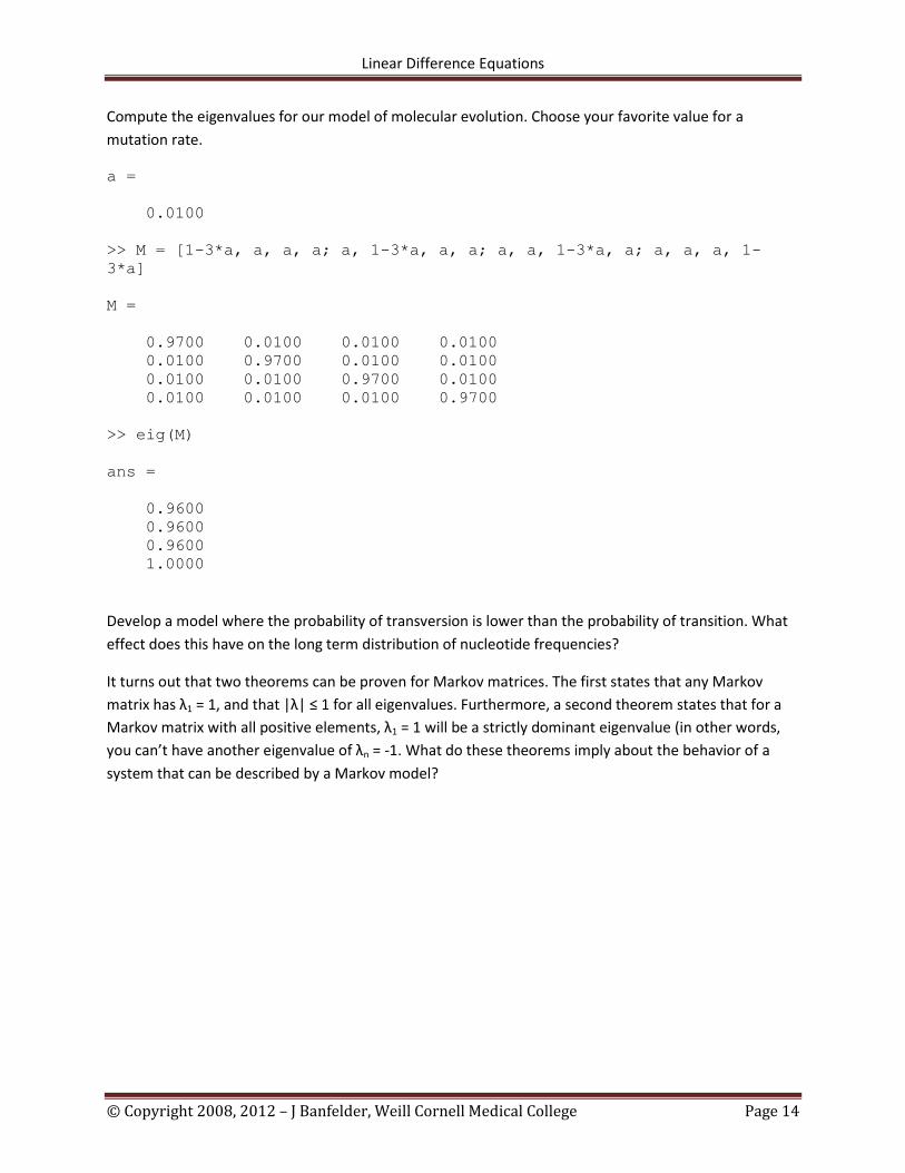
Compute the eigenvalues for our model of molecular evolution. Choose your favorite value for a

mutation rate.

a =

0.0100

>> M = [1-3*a, a, a, a; a, 1-3*a, a, a; a, a, 1-3*a, a; a, a, a, 1-

3*a]

M =

0.9700 0.0100 0.0100 0.0100

0.0100 0.9700 0.0100 0.0100

0.0100 0.0100 0.9700 0.0100

0.0100 0.0100 0.0100 0.9700

>> eig(M)

ans =

0.9600

0.9600

0.9600

1.0000

Develop a model where the probability of transversion is lower than the probability of transition. What

effect does this have on the long term distribution of nucleotide frequencies?

It turns out that two theorems can be proven for Markov matrices. The first states that any Markov

matrix has λ1 = 1, and that |λ| ≤ 1 for all eigenvalues. Furthermore, a second theorem states that for a

Markov matrix with all positive elements, λ1 = 1 will be a strictly dominant eigenvalue (in other words,

you can’t have another eigenvalue of λn = -1. What do these theorems imply about the behavior of a

system that can be described by a Markov model?

linear difference equations - weill cornell...

Documents