journal of difference equations and applications

This article was downloaded by:[Seno, Hiromi]On: 15 November 2007Access Details: [subscription number 785185050]Publisher: Taylor & FrancisInforma Ltd Registered in England and Wales Registered Number: 1072954Registered office: Mortimer House, 37-41 Mortimer Street, London W1T 3JH, UK

Journal of Difference Equations andApplicationsPublication details, including instructions for authors and subscription information:http://www.informaworld.com/smpp/title~content=t713640037

A discrete prey-predator model preserving the dynamicsof a structurally unstable Lotka-Volterra modelHiromi Seno aa Department of Mathematical and Life Sciences, Graduate School of Science,Hiroshima University, Higashi-Hiroshima, Japan

First Published on: 09 October 2007To cite this Article: Seno, Hiromi (2007) 'A discrete prey-predator model preservingthe dynamics of a structurally unstable Lotka-Volterra model', Journal of DifferenceEquations and Applications, 13:12, 1155 - 1170To link to this article: DOI: 10.1080/10236190701464996

URL: http://dx.doi.org/10.1080/10236190701464996

PLEASE SCROLL DOWN FOR ARTICLE

Full terms and conditions of use: http://www.informaworld.com/terms-and-conditions-of-access.pdf

This article maybe used for research, teaching and private study purposes. Any substantial or systematic reproduction,re-distribution, re-selling, loan or sub-licensing, systematic supply or distribution in any form to anyone is expresslyforbidden.

The publisher does not give any warranty express or implied or make any representation that the contents will becomplete or accurate or up to date. The accuracy of any instructions, formulae and drug doses should beindependently verified with primary sources. The publisher shall not be liable for any loss, actions, claims, proceedings,demand or costs or damages whatsoever or howsoever caused arising directly or indirectly in connection with orarising out of the use of this material.

http://www.informaworld.com/smpp/title~content=t713640037

http://dx.doi.org/10.1080/10236190701464996

http://www.informaworld.com/terms-and-conditions-of-access.pdf

Dow

nloa

ded

By:

[Sen

o, H

irom

i] A

t: 01

:24

15 N

ovem

ber 2

007

A discrete prey–predator model preservingthe dynamics of a structurally unstable

Lotka–Volterra model

HIROMI SENO*

Department of Mathematical and Life Sciences, Graduate School of Science, Hiroshima University,Higashi-Hiroshima 739-8526, Japan

(Received 13 July 2006; revised 19 February 2007; in final form 18 May 2007)

Leslie’s method to construct a discrete two dimensional dynamical system dynamically consistent withthe Lotka–Volterra type of competing two species ordinary differential equations is applied in a newlyextended manner for the Lotka–Volterra prey–predator system which is structurally unstable. We showthat, independently of the time step size, the derived discrete prey–predator system is dynamicallyconsistent with the continuous counterpart, keeping the nature of neutrally stable periodic orbit. Further,we show that the extended method to construct the discrete prey–predator system can provide adynamically consistent model also for the logistic Lotka–Volterra one.

Keywords: Lotka–Volterra system; Prey–predator model; Dynamically consistent; Neutrally stable;Population dynamics

1. Introduction

At the end of 1950s, Leslie, who is well-known from his pioneer works of the matrix model

for the structured population [3,4], constructed and numerically analyzed a kind of discrete

two-dimensional dynamical system derived from the familiar Lotka–Volterra type of

competing two species ordinary differential equations (ODE) [5–7]:

dN1ðtÞdt

¼ {r1 2 b11N1ðtÞ2 b12N2ðtÞ}N1ðtÞ;

dN2ðtÞdt

¼ {r2 2 b21N1ðtÞ2 b22N2ðtÞ}N2ðtÞ;

8<: ð1Þ

where Ni(t) (i ¼ 1, 2) is the population size of species-i. Parameters ri, bij (i, j ¼ 1, 2) are all

positive. ri (i ¼ 1, 2) is the intrinsic growth rate of species i, bii (i ¼ 1, 2) the intra-specific

density effect of species i, and bij (i, j ¼ 1, 2; i – j) the inter-specific density effect, that is,

the competition effect from species j to species i. For the ODE system (1), Leslie [5]

considered the following discrete two dimensional system:

N1ðt þ hÞ ¼ 11þf1ðhÞ{b11N1ðtÞþb12N2ðtÞ}

er1hN1ðtÞ;

N2ðt þ hÞ ¼ 11þf2ðhÞ{b21N1ðtÞþb22N2ðtÞ}

er2hN2ðtÞ;

8<: ð2Þ

Journal of Difference Equations and Applications

ISSN 1023-6198 print/ISSN 1563-5120 online q 2007 Taylor & Francis

http://www.tandf.co.uk/journals

DOI: 10.1080/10236190701464996

*Tel./Fax: þ 81-82-424-7394. Email: [email protected]

Journal of Difference Equations and Applications,

Vol. 13, No. 12, December 2007, 1155–1170

Dow

nloa

ded

By:

[Sen

o, H

irom

i] A

t: 01

:24

15 N

ovem

ber 2

007

where

fiðhÞ ¼erih 2 1

riði ¼ 1; 2Þ;

and h is the size of time step.

Surprisingly, his discrete system (2) qualitatively conserves the characteristics of the

solution of the original ODE system (1) even with sufficiently large time step size h, that is,

(2) is a dynamically consistent discrete system for the ODE system (1) [2,8–10,12,13].

Therefore, Leslie’s idea to construct the difference equations from the ODEs might serve as

an alternative and satisfactory numerical scheme for numerical investigation about nonlinear

ODE system.

Different from the usual discretization scheme for ODE (for instance, by Euler method),

Leslie’s idea to derive (2) from (1) is specific and intuitive since it significantly depends on

the idea of mathematical modelling concerning to the original ODE system. His idea is

originally inspired by the relationship between the logistic equation and its exactly

corresponding difference equation. For the logistic equation with positive coefficient b of

intra-specific density effect on the per capita growth rate:

dNðtÞ

dt¼ {r 2 bNðtÞ}NðtÞ; ð3Þ

we can easily obtain the following exact solution with the initial population size N(0):

NðtÞ ¼1

1þ fðtÞbNð0ÞNð0Þert; ð4Þ

where f(t) ¼ (ert 2 1)/r. Making use of the exact solution (4), we can immediately obtain

the corresponding exact discrete model with an arbitrary time step size h as follows (k ¼ 0, 1,

2, . . . ):

Nkþ1 ¼erhNk

1þ fðhÞbNk

ð5Þ

with N0 ¼ N(0). This is a discrete model sometimes called “Verhulst model” or “ Beverton–

Holt model”. Independently of the sign of r, the exact discrete model (5) can exactly trace the

solution (4) with same parameter values, for any time step size h.

Seno [14] has investigated the Leslie’s idea from the viewpoint of the dynamical

consistency with respect to the general single-species model given by the following ODE and

the counterpart difference equation:

dNðtÞ

dt¼ {r 2 QðNðtÞÞ}NðtÞ; Nkþ1 ¼

erhNk

1þ fðhÞQðNkÞ; ð6Þ

where the parameter r is positive, and the function Q is assumed to be non-negative and

sufficiently smooth. It was shown that, independently of the time step size h, the qualitative

behavior around trivial equilibria is consistent between them, and, if

0 ,d½logQðNÞ�

d½logN�

��N¼N *

# 1; ð7Þ

so is that around the non-trivial equilibrium.

H. Seno1156

Dow

nloa

ded

By:

[Sen

o, H

irom

i] A

t: 01

:24

15 N

ovem

ber 2

007

Although Leslie’s idea was inspired by the idea of mathematical modelling concerning to

the original ODE system, the derived discrete system could provide a possibly appropriate

form as a mathematical model for a generational variation of interacting populations. Except

for few models including well-known Nicholson–Bailey model [11], it have attracted little

mathematical attention what mathematical description would be appropriate to describe a

density effect or an intra/inter-specific reaction in a time step (generation) specified in the

discrete model. Especially with respect to the multi species system, the relationship between

the ODE model and the discrete model has been considered much little.

In this paper, in contrast to previous researches about such discrete systems dynamically

consistent with the continuous counterpart from the viewpoint of some nonstandard

discretization method (for example, [2,8–10,12,13]), we consider an extension of Leslie’s

idea for the Lotka–Volterra prey–predator model, and present a new discrete prey–predator

system dynamically consistent with the original ODE model, even when the original one is

structurally unstable.

2. From ODE to time-discrete model

The following Lotka–Volterra prey–predator model is well-known from its structurally

unstable nature (e.g. see [1]):

dHðtÞdt

¼ rHðtÞ2 bHðtÞPðtÞ;

dPðtÞdt

¼ cbHðtÞPðtÞ2 dPðtÞ;

8<: ð8Þ

where H(t) and P(t) are respectively population sizes of prey and predator. r is the intrinsic

(malthusian) growth rate of prey, d the natural death rate of predator. b is the predation

coefficient, c the energy conversion rate from the predation to the predator’s reproduction.

From (8), we can easily find that the following function of populations H and P, which

value is kept constant independently of time [1]:

VðH;PÞ ¼ cbH 2 d logH þ bP2 r logP: ð9Þ

The constant value is determined by the initial state (H(0), P(0)). Indeed, the ODE system

(8) has the infinite number of periodic orbits depending on the initial state, and each periodic

orbit in the phase space is given by V(H, P) ¼ V(H(0), P(0)) (figure 1).

Now, we present the following discrete system dynamically consistent with the original

ODE system (8) as we will show in the subsequent analysis:

Hkþ1 ¼erhHk

1þfH ðhÞbPk;

Pk ¼edhPkþ1

1þfPðhÞcbHkþ1;

8><>: ð10Þ

where

fHðhÞ ¼erh 2 1

r; fPðhÞ ¼

edh 2 1

d

and h is the time step size.

Dynamically consistent discrete prey–predator model 1157

Dow

nloa

ded

By:

[Sen

o, H

irom

i] A

t: 01

:24

15 N

ovem

ber 2

007

The first equation for the prey in (10) is built along the method of Leslie [5–7]. In contrast,

the second equation for the predator in (10) is built with our method newly extended from the

Leslie’s idea: The equation for the predator in the ODE system (8) can be written as follows:

dPðtÞ

d½2t�¼ dPðtÞ2 cbHðtÞPðtÞ:

The form in the right side of this equation corresponds to that in the right side of the

equation for the prey in (8), and is adoptable for the Leslie’s method of building

the corresponding discrete equation, except for the variables H and P of 2 t instead of t.

Since the use of 2 t indicates the temporal inversion as t increases, we put the temporal

relation inverse as shown by the second equation in (10), applying the Leslie’s method to

build the corresponding discrete equation. Similarly as in Leslie’s case, this extension of the

method to build a discrete equation corresponding to an ODE is still intuitive. However, it

surprisingly works well as we will show in the following analysis.

Now the system (10) can be rewritten as follows:

Hkþ1 ¼ erhHk{12PhðPkÞ};

Pkþ1 ¼ e2dh Pk þ c fPðhÞfH ðhÞ

erhHkPhðPkÞn o

;

8<: ð11Þ

where

PhðPkÞ ¼fHðhÞbPk

1þ fHðhÞbPk

: ð12Þ

We can easily find that the discrete system (11) converges to the ODE system (8) as h ! 0.

We can regard (11) as the discrete prey–predator system characterized by the predation

probability Ph per prey in the time interval h, given by (12), and the corresponding energy

conversion rate from the predation to the predator’s reproduction, given by cfP(h)/fH(h).

SincefH(h)/h ! 1 as h ! 0,Ph(Pk)/h converges to bPk. Therefore, the predation probability

Ph given by (12) can be regarded as providing the predation effect appropriately corresponding

Figure 1. Numerically obtained trajectories in the phase plane (H, P) for the ODE system (8) and the discretesystem (11). Trajectories from some different initial points (white circles) are drawn. Dashed thin curves are for (8)and the darker thick plots for (11). (a) h ¼ 0.5 to the 1500th step and (b) h ¼ 20.0 to the 3000th step. r ¼ 1.0;b ¼ 1.0; c ¼ 0.01; d ¼ 0.1.

H. Seno1158

Dow

nloa

ded

By:

[Sen

o, H

irom

i] A

t: 01

:24

15 N

ovem

ber 2

007

to the predation term in the ODE system (8). The energy conversion rate in the discrete model

(11) converges to c as h ! 0, which exactly corresponds to that in the ODE model (8), too.

These features of the discrete model (11) are very interesting from the viewpoint of

mathematical modelling for the time-discrete variation of population size. The predation

probability Ph is a rational function of bP, which is monotonically increasing in terms of bP

with the upper bound 1. Hence the ratio of predated prey population is not proportional to the

predator population size in the time-discrete model. In contrast, in the ODE model (8),

the momental predation rate is proportional to the predator population size at each moment,

because of the mass-action type of predation term. In fact, such mass-action type of predation

term in the ODEmodel does not mean the linear relationship of the decrease of prey population

size due to the predation. It results in a non-linear characteristics of the decrease of prey

population size. In our derivation of a dynamically consistent discrete prey–predator model,

we can regard that such non-linearity of the decrease of prey population size due to the

predation would be reflected to the form of a rational function for the predation probabilityPh.

2.1 Existence and stability of equilibria

It is easily shown that the systems of (8) and (11) have the common equilibria: (0, 0) and

(d/a, r/b). No other equilibrium exists. As for the trivial equilibrium (0, 0), the eigenvalues

for (8) are r and2d while erh and e2dh for (11). Therefore, for both systems of (8) and (11),

the equilibrium (0, 0) is unstable as a saddle point, independently of the time step size h.

As for the non-trivial equilibrium (d/a, r/b), the eigenvalues for (8) is given by ^iffiffiffiffiffird

p.

So the equilibrium (d/a, r/b) has the neutral stability for (8). In comparison, the eigenvalue l

for the equilibrium (d/a, r/b) of (11) is given by the roots of the following characteristic

equation:

l2 2 ð1þ e2rh þ e2dh 2 e2rhe2dhÞlþ 1 ¼ 0: ð13Þ

Since the discriminant for this equation is given by

2ð1 2 e2rhÞð1 2 e2dhÞð3 þ e2rh þ e2dh 2 e2rhe2dhÞ , 0;

the eigenvalues are always complex. Further from the characteristic equation (13), we can

easily find that the absolute value of the eigenvalue is 1. The unity of the absolute value of the

eigenvalue means that the stability of the equilibrium (d/a, r/b) of (11) is neutral as that of

(8), again independently of the time step size h.

As indicated by the numerical calculation of trajectories in the phase plane (H, P) in

figure 1, the sequence of points given by (11) is on a closed curve determined by the initial

point in the phase plane. This can be regarded as a nature dynamically consistent with the

original ODE system (8) which has the periodic orbit V(H, P) ¼ V(H(0), P(0)) defined by (9).

On the other hand, from a mathematical viewpoint, the discrete system (11) shows a sort of

chaotic variation. Although figure 2 might be quasi-periodic, it does not, because the

trajectory in the phase plane appears dense on a closed curve as shown in figure 1. However,

the numerically estimated Lyapnov exponent results in nearly zero instead of positive.

2.2 Numerical estimation of the difference from the ODE counterpart

In this section, we numerically investigate the quantitative difference between the behaviors

of the discrete system (11) and the ODE one (8). Although we have seen the qualitative


Dow

nloa

ded

By:

[Sen

o, H

irom

i] A

t: 01

:24

15 N

ovem

ber 2

007

correspondence between them in the previous section, the quantitative difference between

them could be relevant, for instance, as a nonstandard discretization method for the ODE

system (8).

As seen in figure 2, the variation of population sizes for (8) and (11) is quantitatively

different from each other in terms of their values at each moment, whereas the qualitative

nature is consistent as shown in the previous section. In fact, as shown in figure 3, the

distance between points of (8) and (11) in the phase plane (H, P) appears oscillatory.

Numerical results imply that the actual velocity of moving on a closed curve in the phase

plane is different about these two systems even with the same parameter values. We can see

that the velocity is higher for the discrete system (11) than for the ODE system (8).

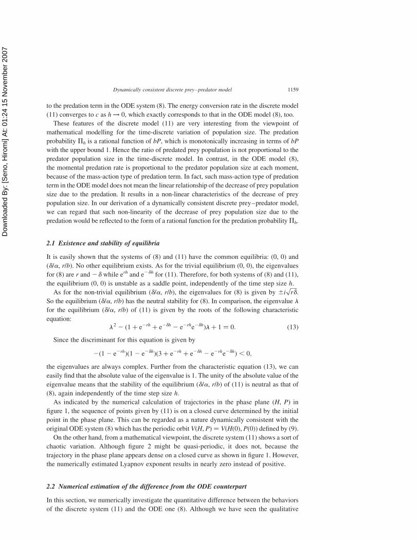
To investigate numerically the h-dependence of the difference in terms of the distance

between points of (8) and (11) in the phase plane (H, P), we consider the following time-

averaged difference of the distance:

Figure 3. Numerically obtained variation of the distance between points of (8) and (11) in the phase plane (H, P).(a) h ¼ 0.1 and (b) h ¼ 0.5. Commonly, r ¼ 1.0; b ¼ 1.0; c ¼ 0.01; d ¼ 0.1; H(0) ¼ H0 ¼ 10.0; P(0) ¼ P0 ¼ 0.5.

Figure 2. Numerically obtained variation of H and P to the 300th step. Thick curve is for the ODE system (8), andthe thin with black plots is for the discrete system (11). r ¼ 1.0; b ¼ 1.0; c ¼ 0.01; d ¼ 0.1; h ¼ 0.5;H(0) ¼ H0 ¼ 10.0; P(0) ¼ P0 ¼ 0.6.

H. Seno1160

Dow

nloa

ded

By:

[Sen

o, H

irom

i] A

t: 01

:24

15 N

ovem

ber 2

007

Ed ¼ limn!1

1

n

Xnk¼1

ffiffiffiffiffiffiffiffiffiffiffiffiffiffiffiffiffiffiffiffiffiffiffiffiffiffiffiffiffiffiffiffiffiffiffiffiffiffiffiffiffiffiffiffiffiffiffiffiffiffiffiffiffiffiffiffiffiffiffiffiffiffiffiffi{Hk 2 HðkhÞ}2 þ {Pk 2 PðkhÞ}2

q: ð14Þ

Numerically estimated value of Ed is shown in figure 5. Our numerical calculations

indicate that the value of Ed tends to increase in terms of h. This means that the trajectory of

the discrete system (11) becomes quantitatively more different from the trajectory of the

ODE system (8) with the same initial state. This can be seen also in figure 2. It is natural that

the value Ed also depends on the initial state (H0, P0). Besides, since each trajectory is on a

closed curve, the averaged difference Ed is bounded.

As another comparison between them, we investigate the temporal variation in the value of

the function V(H, P) defined by (9), since it temporally keeps a constant value V(H(0), P(0))

determined by the initial state in case of the ODE system (8). As shown in figure 4, its

variation is oscillatory for the discrete system (11), too, and however has relatively small

values in its temporal variation. As we can see in figure 1(a), the closed curve on which the

trajectory of the discrete system (11) for a small h (even though still relatively large from the

viewpoint of numerical calculation approximating the ODE system (8)) has a little difference

from that of the ODE system (8), while the difference becomes greater as the time step size h

gets larger.

To investigate numerically the h-dependence of the difference of the value of V(H, P) for

the discrete system (11), we consider the following time-averaged difference of the value of

V(H, P):

EV ¼ limn!1

1

VðH0;P0Þ

ffiffiffiffiffiffiffiffiffiffiffiffiffiffiffiffiffiffiffiffiffiffiffiffiffiffiffiffiffiffiffiffiffiffiffiffiffiffiffiffiffiffiffiffiffiffiffiffiffiffiffiffiffiffiffiffiffiffiffiffiffiffi1

n

Xnk¼1

{VðHk;PkÞ2 VðH0;P0Þ}2

s: ð15Þ

Numerically estimated value of EV is shown in figure 5. Our numerical calculations

indicate that the value of EV is monotonically increasing in terms of h. This means that the

closed curve on which the trajectory of the discrete system (11) is located is more different

from the closed orbit of the ODE system (8) with the same initial state as the time step size h

gets larger. This can be seen also in figure 1. It is natural that the value EV also depends on

the initial state (H0,P0). Besides, since each trajectory is on a closed curve, the averaged

difference EV is bounded.

Figure 4. Numerically obtained variation of the difference of the value of function V(H, P), defined by (9), for thediscrete system (11). The value of {V(Hk, Pk) 2 V(H0, P0)}/V(H0 P0) is plotted. (a) h ¼ 0.1 to the 2500th step and(b) h ¼ 0.5 to the 500th step. Commonly, r ¼ 1.0; b ¼ 1.0; c ¼ 0.01; d ¼ 0.1; H0 ¼ 10.0; P0 ¼ 0.5.


Dow

nloa

ded

By:

[Sen

o, H

irom

i] A

t: 01

:24

15 N

ovem

ber 2

007

2.3 General form of the discrete 1 prey-1 predator model

From the discrete system (11), we can derive the following general form of the discrete 1

prey-1 predator model:

Xkþ1 ¼ R Xk 2XkYk

1þYk

� �;

Ykþ1 ¼ DYk þXkYk

1þYk:

8><>: ð16Þ

Parameters R and D are positive with D , 1. This system can be derived from (11) with

the following transformation of variables and parameters: Xk ¼ cbfP(h)erhHk;

Xkþ1 ¼ cbfP(h)erhHkþ1; Yk ¼ fH(h)bPk; Ykþ1 ¼ fH(h)bPkþ1; R ¼ erh; D ¼ e2dh.

Although these parameters are not independent of each other in terms of h, we here

consider more generally the case when these parameters R and D are independent.

The confinement of D , 1 is a modelling requirement. As a dynamics of

predator population growth, the predator population can grow only with the predation.

If D . 1, Yk ! 1 as k ! 1 even without the prey, since Ykþ1 . Yk for any k.

Now the parameter D means the natural death rate for the predator, so that we assume

hereafter that D , 1.

The system (16) has only two equilibria: (0, 0) and (R(1 2 D), R 2 1). The non-trivial

POSITIVE equilibrium (R(1 2 D), R 2 1) exists if and only if D , 1 and R . 1. If

R , 1 and D , 1, the trivial equilibrium (0, 0) is locally stable. As in case of the discrete

system (11), even in this general case of (16), the stability of the non-trivial

positive equilibrium is neutral whenever it exists. Numerical calculations show that the

trajectory for (16) is always on a closed curve, as in case of (11), independently of

parameter values. Therefore, the general form of discrete population dynamics given

by (16) can be regarded as dynamically consistent with the Lotka–Volterra prey–predator

system (8).

Consequently, we can regard the model of the prey–predator population dynamics given

by (16) as a time-discrete version corresponding to the Lotka–Volterra prey–predator model

(8). Further, we could regard the prey–predator reaction term given by a rational function in

(16) as a temporally integrated (over the period of the discrete time step) mass-action type of

prey–predator reaction, because of the correspondence with the mass-action term in the

ODE model (8).

Figure 5. Numerically obtained h-dependence of the averaged difference Ed and EV , respectively, defined by (14)and (15), between the ODE system (8) and the discrete one (11), according to the trajectory in the phase plane (H, P).r ¼ 1.0; b ¼ 1.0; c ¼ 0.01; d ¼ 0.1; H0 ¼ 10.0; P0 ¼ 0.5.

H. Seno1162

Dow

nloa

ded

By:

[Sen

o, H

irom

i] A

t: 01

:24

15 N

ovem

ber 2

007

3. Application for a more general structurally unstable system of prey–predator type

In this section, we consider a family of general prey–predator ODE system given by

dXðtÞdt

¼ rXðtÞ2 f ðYðtÞÞXðtÞ

dYðtÞdt

¼ gðXðtÞÞYðtÞ2 dYðtÞ;

8<: ð17Þ

where functions f and g are assumed to be sufficiently smooth and satisfy that f(x) $ 0 and

g(x) $ 0 for any x . 0 with f(0) ¼ g(0) ¼ 0.

Our method to construct the corresponding discrete system gives the following:

Xkþ1 ¼erhXk

1þfH ðhÞ f ðYkÞ;

Yk ¼edhYkþ1

1þfPðhÞgðXkþ1Þ;

8><>:

that is,

Xkþ1 ¼ erhXk{12PhðYkÞ};

Ykþ1 ¼ e2dh{Yk þ fPðhÞgðXkþ1ÞYk};

(ð18Þ

where

PhðYkÞ ¼fHðhÞ f ðYkÞ

1þ fHðhÞ f ðYkÞ:


It can be easily seen that the ODE prey–predator system (17) and the discrete system (18)

have the following common equilibria and do not have any other: (0, 0) and (X *, Y *), where

the coexistent equilibrium (X *, Y *) can exist if and only if the following equations have

positive roots:

f ðY *Þ ¼ r;

gðX *Þ ¼ d:

(

As for the trivial equilibrium (0, 0), the eigenvalues for (17) are r and 2d while erh and

e2dh for (18). Therefore, for both systems of (17) and (18), the equilibrium (0, 0) is unstable

as a saddle point, independently of the time step size h.

Next, let us consider the case when a non-trivial equilibrium (X *, Y *) exists. In this case,

the eigenvalues for the ODE system (17) are given by ^ffiffiffiffiffiffiffiffiffiffiffiffiffiffiffiffiffiffiffiffiffiffiffiffiffiffiffiffiffiffiffiffiffiffiffiffiffiffiffiffiffi2f 0ðY *Þg 0ðX *ÞX *Y *

p. Therefore,

for the ODE system (17), the coexistent equilibrium (X *, Y *) is unstable if f 0(Y *)g 0(X *) , 0

as a saddle, while neutrally stable with purely imaginary eigenvalues if f 0(Y *)g 0(X *) . 0.

As for the discrete system (18), the eigenvalue l for the coexistent equilibrium (X *, Y *) is

given by the root of the following characteristic equation:

l2 2 ð22 ABÞlþ 1 ¼ ðl2 1Þ2 2 ABl ¼ 0;


Dow

nloa

ded

By:

[Sen

o, H

irom

i] A

t: 01

:24

15 N

ovem

ber 2

007

where

A ¼ e2rhfHðhÞf0ðY *ÞX *; B ¼ e2dhfPðhÞg

0ðX *ÞY *:

From the above characteristic equation, we can find that the coexistent

equilibrium (X *, Y *) of the discrete system (18) is unstable if f 0(Y *)g 0(X *) , 0 as

a saddle with positive eigenvalues, one of which is less than 1 and the other more than 1.

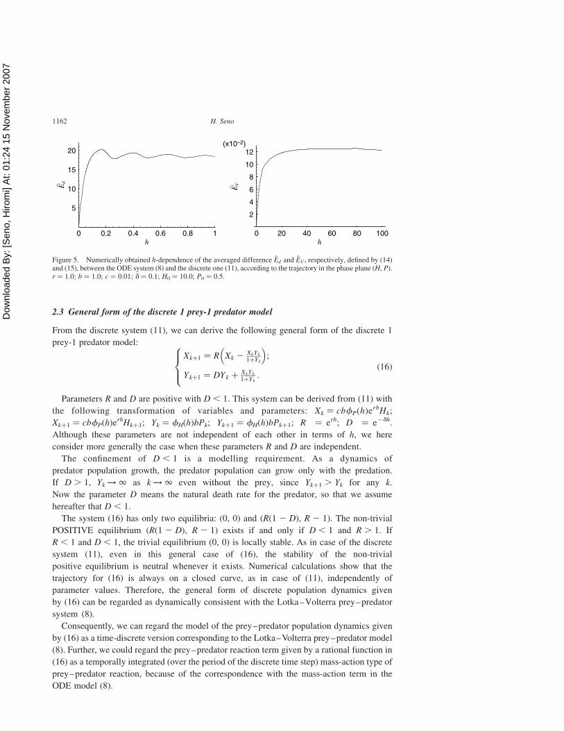
When f 0(Y *)g 0(X *) . 0, if

f 0ðY *Þg 0ðX *ÞX *Y * , CðhÞ ¼4eðrþdÞh

fHðhÞfPðhÞ; ð19Þ

the eigenvalues are complex with the absolute value 1, so that the equilibrium is neutrally

stable. In contrast, when f 0(Y *)g 0(X *) . 0, if f 0(Y *)g 0(X *)X *Y * . C(h), the eigenvalues

are negative, one of which is less than 21 and the other more than 21, so that it is a saddle

again. In this case, the dynamical consistency breaks down between (17) and (18). Since

C(h) is monotonically decreasing in terms of h and limh!0

CðhÞ ¼ 1, this inconsistency cannot

occur for sufficiently small time step size h but can do for relatively large time step size h,

depending on the characteristics of functions f and g. For example, the following f and g give

an example for such a case of the dynamical consistency breaking down (figure 6):

f ð yÞ ¼ 5y; gðxÞ ¼x12

1þ x 12: ð20Þ

In this case, the discrete system (18) shows a chaotic oscillation for sufficiently large time

step size h.

Figure 6. Numerically obtained trajectories in the phase plane (H, P) for the ODE system (17) and the discrete one(18) with (20). Uniquely determined coexistent equilibrium is indicated by a black point. The thin curve is for (17)and the darker plots to the ten thousandth step for (18). (a) h ¼ 0.5, (b) h ¼ 1.0, (c) h ¼ 2.0, (d) h ¼ 2.5, (e) h ¼ 2.65and (f) h ¼ 5.0. Commonly, r ¼ 1.0; d ¼ 0.5; H0 ¼ 0.99; P0 ¼ 0.25.

H. Seno1164

Dow

nloa

ded

By:

[Sen

o, H

irom

i] A

t: 01

:24

15 N

ovem

ber 2

007

Since C(h) further satisfies that limh!1

CðhÞ ¼ rd, if f 0(Y *)g 0(X *)X *Y * # rd ¼ f(Y *)g(X *),

that is, if

d½log f ðyÞ�

d½log y�

��y¼Y *

d½log gðxÞ�

d½log x�

��x¼X *

# 1; ð21Þ

then the condition (19) is always satisfied so that the coexistent equilibrium (X *, Y *) is

neutrally stable, independently of the time step size h, when f 0(Y *)g 0(X *) . 0. The condition

(21) appears the extension of the corresponding (7) for the one-dimensional case (6)

discussed by Seno [14]. Lastly, if the condition (21) is satisfied for every equilibrium, then

the discrete system (18) is dynamically consistent with the ODE system (17) according to the

existence and the local stability of equilibria, independently of the time step size.

4. Application for the Lotka–Volterra prey–predator system with logistically growing

prey

In this section, as a natural extended ODE model from (8), we consider the following ODE

system with logistically growing prey:

dHðtÞdt

¼ {r 2 bHðtÞ}HðtÞ2 bHðtÞPðtÞ;

dPðtÞdt

¼ cbHðtÞPðtÞ2 dPðtÞ:

8<: ð22Þ

Analogously to the discrete system (10), we now present the following discrete system as a

corresponding discrete model:

Hkþ1 ¼erhHk

1þfH ðhÞ{bHkþbPk};

Pk ¼edhPkþ1

1þfPðhÞcbHkþ1;

8><>:

that is,

Hkþ1 ¼ erhHk{12 GhðHk;PkÞ2PhðHk;PkÞ};

Pkþ1 ¼ e2dh Pk þ c fPðhÞfH ðhÞ

erhHk�PhðHk;PkÞn o

;

8<: ð23Þ

where

GhðHk;PkÞ ¼fHðhÞbHk

1þ fHðhÞbHk þ fHðhÞbPk

; ð24Þ

PhðHk;PkÞ ¼fHðhÞbPk

1þ fHðhÞbHk þ fHðhÞbPk

: ð25Þ

From the obtained form of the discrete system (23), we can see that the function Gh

represents the contribution of the logistic density effect on the prey population growth in the

period h, and the function Ph does that of the predation. Differently from the predation

probability (12) in the previous discrete model (11), the functionPh of (25) depends also on the

prey population size Hk. We can consider that this would be an effect of the logistic density

effect on the predation efficiency since the reduction of prey density is reflected to the net


Dow

nloa

ded

By:

[Sen

o, H

irom

i] A

t: 01

:24

15 N

ovem

ber 2

007

growth rate through the density effect while the predation to reduce the prey density depends

on the prey density itself. Simultaneously the density effect function Gh of (24) depends on the

predator population size. This can be regarded as to reflect the effect of predation which

decreases the prey density and then reduces the density effect in the period h.


It can be easily seen that the ODE system (22) and the discrete system (23) have the

following common three equilibria: (0, 0), (r/b, 0), and (d/(cb), (rcb 2 bd)/(cb 2)).

The extinction equilibrium (0, 0) is unstable as a saddle point for both systems because the

eigenvalues are r and2d for theODEsystem (22)while erh and e2dh for the discrete system (23).

As for the predator extinction equlibrium (r/b, 0), the eigenvalues are r and rcb/(b) 2 d

for the ODE system (22) while e2rh and

ð1 2 e2dhÞrcb

bdþ e2dh

for the discrete system (23). In both cases, we find that the equilibrium is a locally stable node

if bd/rcb . 1. If bd/rcb , 1, it is a saddle in both cases. Hence, also as for the stability of the

predator extinction equlibrium (r/b, 0), the discrete system (23) is dynamically consistent

with the ODE system (22).

As for the coexistent equilibrium (d/(cb), (rcb 2 bd)/(cb 2)), we consider its stability

under the following condition for its positiveness: bd/rcb , 1. If this positiveness condition

is satisfied, the predator extinction equilibrium (r/b, 0) is always unstable, that is, if the

coexistent equilibrium exists, the predator extinction equilibrium is not feasible.

The eigenvalue l of the coexistent equilibrium for the ODE system (22) is given by the

following characteristic equation:

l2 þbd

cblþ rd 12

bd

rcb

� �¼ 0:

We can easily find that the coexistent equilibrium (d/(cb), (rcb 2 bd)/(cb 2)) for the ODE

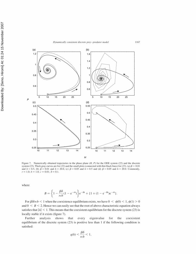
system (22) is locally stable whenever it exists (figure 7). Further, from the above

characteristic equation, we find that, if

bd

rcb,

2

1 þffiffiffiffiffiffiffiffiffiffiffiffiffiffiffiffi1 þ r=d

p ;

the coexistent equilibrium (d/(cb), (rcb 2 bd)/(cb 2)) is a stable focus (figure 7(a),(b)), while,

if

2

1 þffiffiffiffiffiffiffiffiffiffiffiffiffiffiffiffi1 þ r=d

p #bd

rcb, 1;

it is a stable node (figure 7(c),(d)).

In contrast, the eigenvelue l of the coexistent equilibrium for the discrete system (23) is

given by the following characteristic equation:

cðlÞ ¼ l2 2 Blþ 12bd

rcbð12 e2rhÞ ¼ 0;

H. Seno1166

Dow

nloa

ded

By:

[Sen

o, H

irom

i] A

t: 01

:24

15 N

ovem

ber 2

007

where

B ¼ 12bd

rcbð12 e2rhÞ

� �e2dh þ {1þ ð12 e2dhÞe2rh}:

For bd/rcb , 1 when the coexistence equilibrium exists, we have 0 , c(0) , 1, c(1) . 0

and 0 , B , 2. Hence we can easily see that the root of above characteristic equation always

satisfies that jlj , 1. This means that the coexistent equilibrium for the discrete system (23) is

locally stable if it exists (figure 7).

Further analysis shows that every eigenvalue for the coexistent

equilibrium of the discrete system (23) is positive less than 1 if the following condition is

satisfied:

qðhÞ ,bd

rcb, 1;

Figure 7. Numerically obtained trajectories in the phase plane (H, P) for the ODE system (22) and the discretesystem (23). Thick gray curves are for (22) and the small plots (connected with thin black lines) for (23). (a) b ¼ 0.01and h ¼ 0.5, (b) b ¼ 0.01 and h ¼ 20.0, (c) b ¼ 0.05 and h ¼ 0.5 and (d) b ¼ 0.05 and h ¼ 20.0. Commonly,r ¼ 1.0; b ¼ 1.0; c ¼ 0.01; d ¼ 0.1.


Dow

nloa

ded

By:

[Sen

o, H

irom

i] A

t: 01

:24

15 N

ovem

ber 2

007

where

qðhÞ ¼ 1212 e2rhffiffiffiffiffiffiffiffiffiffiffiffiffiffiffiffiffiffi

12 e2dhp

þffiffiffiffiffiffiffiffiffiffiffiffiffiffiffiffiffiffiffiffiffiffiffiffi12 e2ðrþdÞh

pn o2:

In this case, the coexistence equilibrium of the discrete system (23) is a stable node.

If bd/rcb , q(h), every eigenvalue is complex with its absolute value less than 1, so that the

coexistence equilibrium of the discrete system (23) is a stable focus. We can easily find that

qðhÞ! 2=ð1 þffiffiffiffiffiffiffiffiffiffiffiffiffiffiffiffiffi1 þ r=d

pÞ as h ! 0, and q(h) ! 3/4 as h ! 1.

From these results, although the dynamical behaviors of the ODE system (22) and the

discrete one (23) are mostly consistent, the subtle nature of the bifurcation with respect to

the stability of coexistent equilibrium is affected by the value of time step size h (figures 7(d)

and 8). However, since q(h) has a finite limit of the value 3/4 as shown in the above,

surprisingly the difference of the bifurcation boundary is bounded for any time step size h

(figure 8). In this sense, the dynamical consistency between the ODE system (22) and the

discrete one (23) would be regarded as rather robust against the time step size h.

5. Conclusion and future directions

Our method to construct a discrete prey–predator system from the ODE model successfully

provides a dynamically consistent model which could have a structure explicitly translatable

in ecological meanings from the viewpoint of mathematical modelling. Although our method

is somehow intuitive as Leslie’s, the mathematical formulas in the constructed model would

be appropriate expression of the intra/inter-specific density effect on the population

Figure 8. A numerical example of the h-dependence of the bifurcation between the stable node and the stable focusaccording to the coexistent equilibrium of (22) and (23). Region (F, F) indicates that both the ODE and the discretesystems show the stable focus, and (N, F) does that the ODE system shows the stable node while the discrete onedoes the stable focus. The other symbols are similarly defined. (a) b ¼ 0.3, (b) b ¼ 0.5, (c) b ¼ 0.6 and (d) b ¼ 1.0.Commonly r ¼ 1.0.

H. Seno1168

Dow

nloa

ded

By:

[Sen

o, H

irom

i] A

t: 01

:24

15 N

ovem

ber 2

007

dynamics in a discrete time step. For further example, some numerical and mathematical

analyses show that our method would be valid also for the Kermack–McKendrick SIR

model, which we did not describe in this paper.

In history, lots of ODE models have been successful to explain or describe biological

phenomena even when those phenomena are fundamentally composed of time-discrete or

temporally discontinuous events. Generally we could have any data in a discrete time step or

analyze only such a sequence of data. In these reasons, some successful ODE models would be

expected to provide some informations useful to find an appropriate structure of time-discrete

model which explains or describes the biological phenomena. Especially in the theory of

population dynamics, the essential structure of any mathematical model depends on the

expression of intra/inter-specific interaction. Hence it is very important how the density effect

is involved in the model. However, we have had little knowledge or discussion about the

appropriate formulas of some density effect in the discrete model, although some discrete

models derived from the ODE counterpart model with a discretization method have been

successful. We expect that our result would be helpful to develop some theory or discussion

about this subject.

As another aspect, since our method to construct a discrete system from the ODE

counterpart is newly discussed here, it would be helpful for some discussion about some

nonstandard discretization method which could provide a discrete system robustly

dynamically consistent with the original ODE system. Recently some works have been done

on the nonstandard discretization of the Lotka–Volterra prey–predator model that can

preserve the unstable structure of the original ODE system [2,8–10,12,13]. Those works

have focused the algorithmic way of the dynamically consistent discretization for the ODE

system with the polynomial (especially mass-action) type of reaction terms. Roeger [13]

discussed the generalization of the dynamically consistent discretization originally proposed

by Mickens [9] for the Lotka–Volterra system, though there was no discussion about the

meanings or the perspectives as the discrete model of population dynamics with some

specific density effect. In her paper, the discrete prey–predator system corresponding to ours,

(11) with (12), appears as a specific case, although there was a difference about the

contribution of the time step size h in the discrete system. Moreover her and the other

previous works did not mention the idea and the intuitive way of discretization by Leslie and

Gower [5–7], and independently discussed the dynamically consistent discretization.

Since the aim of this paper is to discuss the structure of a discrete model corresponding to

the Lotka–Volterra prey–predator model, we do not discuss in this paper any more the

further generalization of our method to construct a discrete system. It is very interesting to

extend our method, for instance, to a multi species (more than one prey or predator) system or

to a more general family of 1 prey-1 predator system. It is one of the next steps of our work.

References

[1] Britton, N.F., 2003, Essential Mathematical Biology (London: Springer-Verlag).[2] Cushing, J.M., Levarge, S., Chitnis, N. and Henson, S.M., 2004, Some discrete competition models and the

competitive exclusion principle. Journal of Difference Equations and Applications, 10, 1139–1151.[3] Leslie, P.H., 1945, On the use of matrices in certain population mathematics. Biometrika, 33, 183–212.[4] Leslie, P.H., 1948, Some further notes on the use of matrices in population mathematics. Biometrika,

35, 213–245.[5] Leslie, P.H., 1958, A stochastic model for studying the properties of certain biological systems by numerical

methods. Biometrika, 45, 16–31.


Dow

nloa

ded

By:

[Sen

o, H

irom

i] A

t: 01

:24

15 N

ovem

ber 2

007

[6] Leslie, P.H. and Gower, J.C., 1958, The properties of a stochastic model for two competing species. Biometrika,45, 316–330.

[7] Leslie, P.H. and Gower, J.C., 1960, The properties of a stochastic model for tthe prey–predator type ofinteraction between two species. Biometrika, 47, 219–234.

[8] Liu, P. and Elaydi, S.N., 2001, Discrete competitive and cooperative models of Lotka–Volterra type. Ecology,54, 384–391.

[9] Mickens, R.E., 2003, A nonstandard finite-difference scheme for the Lotka–Volterra system. AppliedNumerical Mathematics, 45, 309–314.

[10] Mounim, A.S. and de Dormale, B., 2004, A note on Mickens’s finite-difference scheme for the Lotka–Volterrasystem. Applied Numerical Mathematics, 51, 341–344.

[11] Nicholson, A.J. and Bailey, V.A., 1935, The balance of animal populations. Part I. Proceedings of theZoological Society of London, 1935(3), 551–598.

[12] Roeger, L.-I.W., 2005, A nonstandard discretization method for Lotka–Volterra models that preserves periodicsolutions. Journal of Difference Equations and Applications, 11, 721–733.

[13] Roeger, L.-I.W., 2006, Nonstandard finite-difference schemes for the Lotka–Volterra systems: generalizationof Mickens’s method. Journal of Difference Equations and Applications, 12, 937–948.

[14] Seno, H., 2003, Some time-discrete models derived from ODE for single-species population dynamics: Leslie’sidea revisited. Scientiae Mathematicae Japonicae, 58, 389–398.

H. Seno1170

journal of difference equations and applications

Documents