limitations in direct and indirect methods for solving ...apstrakt: fokus ovog članka je na...

Industrija, Vol.44, No.4, 2016 19

Kruna Ratković1 JEL: C61, O41

DOI: 10.5937/industrija44-10874 UDC: 330.35/.36]:519.8

Original Scientific Paper

Limitations in Direct and Indirect Methods for Solving Optimal Control Problems in

Growth Theory

Article history:

Received: 5 May 2016 Sent for revision: 30 June 2016 Received in revised form: 29 August 2016 Accepted: 7 September 2016 Available online:30 December 2016

Abstract: The focus of this paper is on a comprehensive analysis of different

methods and mathematical techniques used for solving optimal control

problems (OCP) in growth theory. Most important methods for solving

dynamic non-linear infinite-horizon growth models using optimal control theory

are presented and a critical view of the limitations of different methods is

given. The main problem is to determine the optimal rate of growth over time

in a way that maximizes the welfare function over an infinite horizon. The

welfare function depends on capital-labor ratio, the state variable, and the per-

capita consumption, the control variable. Numerical methods for solving OCP

are divided into two classes: direct and indirect approach. How the indirect

approach can be used is given in the example of the neo-classical growth

model. In order to present the indirect and the direct approach simultaneously,

two endogenous growth models, one written by Romer and another by Lucas

and Uzawa, are studied. Advantages and efficiency of these different

approaches will be discussed. Although the indirect methods for solving OCP

are still the most expanded in growth theory, it will be seen that using direct

methods can also be very efficient and help to overcome problems that can

occur by using the indirect approach.

Key words: optimal control, direct and indirect methods, growth theory.

1 University of Donja Gorica, Faculty of Applied Sciences, Montenegro,

[email protected]

mailto:[email protected]

Ratković K.: Limitations in Direct and Indirect Methods for Solving Optimal Control…

20 Industrija, Vol.44, No.4, 2016

Ograničenja u primeni direktnih i indirektnih metoda za

rešavanje problema optimalne kontrole u teoriji rasta

Apstrakt: Fokus ovog članka je na detaljnoj i sveobuhvatnoj analizi glavnih metoda i matematičkih tehnika koje se koriste za rešavanje problema optimalne kontrole u teoriji rasta. Dat je pregled najvažnijih metoda za rešavanje dinamičkih nelinearnih modela rasta koristeći optimalnu kontrolu, kao i kritički osvrt na njihova ograničenja. Osnovni problem koji treba rešiti ovim pristupom je određivanje optimalne stope rasta tokom vremena na način koji maksimizira funkciju blagostanja u beskonačnom vremenskom periodu. Funkcija blagostanja zavisi od koeficijenta kapitalne opremljenosti rada (promjenljive stanja) i od potrošnje po glavi stanovnika (kontrolne promjenljive). Numeričke metode za rešavanje problema optimalne kontrole su podeljene u dve klase: direktni i indirektni pristup. Na primjeru neoklasičnog modela rasta dat je prikaz indirektnog pristupa. Kako bi se predstavio istovremeno indirektni i direktni pristup, u radu će biti data i primena ovih metoda kod dva endogena modela: Romerov i Lucas-Uzawa model. Biće date prednosti i efikasnost jedne metode u odnosu na drugu. Iako se indirektne metode za rešavanje problema optimalne kontrole u ovoj oblasti i dalje najviše upotrebljavaju u praksi, biće viđeno da primjena direktnih metoda može biti vrlo efikasna i korisna u prevazilaženju problema koji se mogu javiti kod indirektnog pristupa.

Ključne reči: optimalna kontrola, direktne i indirektne metode, teorija rasta

1. Introduction

Optimal control theory, as an extension of the calculus of variations,

represents a modern approach to dynamic optimization. Because of the

complexity of most applications, optimal control problems are most often

solved numerically. Numerical methods for solving optimal control problems

date back to the 1950s and the work of Bellman (1957). Since the complexity

and variety of applications has increased over the last decades, the

complexity of methods in optimal control increased as well, such that optimal

control theory has become a discipline that is important to many branches of

economics. Its principal applications in economics are in financial economics,

dynamic macroeconomic theory and resource economics. In particular,

optimal control theory has been applied in growth theory since the article of

Arrow (1968) and later in both exogenous and endogenous growth models

such as Ramsey (1928), Solow (1956), Uzawa (1965), Lucas (1988) and



Romer (1994). Optimal control techniques and the economic interpretation

have been discussed by authors such as Arrow and Kurz (1970), Aghion and

Howitt (1998), Barro and Sala-i-Martin (2003), Cass (1965), Chiang (1992),

Dixit (1990), Dorfman (1969), Intrilligator (1971), Kamien and Schwartz

(1991), Koopmans (1963) and others. Since the same principles are applied

to the new growth models as to the neoclassical growth model, there is a

great literature as an introduction to optimal control techniques (cf. Acemoglu

(2007), Aseev (2009)).

The study of these dynamic growth models follows a usual procedure, which

is to apply Pontryagin's Maximum Principle and to obtain the necessary

optimality conditions, together with the transversality condition. If the initial

values for the state variables are defined, it will give us a complete description

of the system, enough to explain the economy around its steady state. This

formulation gives rise to a system of nonlinear differential equations

describing the economy. Nonlinearity usually arises from the diminishing

marginal utility of consumption and from the diminishing marginal productivity

of the factors of production, but can also be the result of incorporating R&D

(Williams and Jones, 1995) or government spending (Barro, 1990).

Nonlinearity in the production and utility functions and saddle path stability,

can influence the analysis of the transitional dynamics after a structural

change or a policy shock, as (Atolia, Chatterjee, & Turnovsky, 2008) point out.

One way to overcome this problem would be to linearize the dynamic system

around its (post-shock) steady state and then to study this linearized, hence

simplified, version of the dynamic system as an analogue to the original

nonlinear one. But linearization can potentially be fallacious as Wolman and

Couper (2003) noticed. Nevertheless, linearization is still the principal method

used in the growth literature. Consequently, there were some numerical

methods that tried to overcome this problem of linearization such as the

projection method (Judd, 1992), the discretization method (Mercenier &

Michel, 1994), the shooting method (Judd, 1998), the time elimination method

(Mulligan & Sala-i Martin, 1991), the backward integration procedure (Brunner

& Strulik, 2002) and the relaxation procedure (Trimborn, Koch, & Steger,

2004).

All of these numerical methods, together with the linearization, rely on indirect

methods to solve the OCP of the growth model. According to Betts (2001),

indirect methods can sometimes be difficult to apply and the necessary

optimality conditions might be hard to determine explicitly. Economic models



are usually formulated with this in mind and sometimes simplicity is imposed

onto them so that an analytical solution can be found, which is not always the

case.

As opposed to indirect methods, the direct methods solve the OCP in a way

that the OCP is first discretized and then optimized. More precisely, the direct

approach uses the following procedure: the first step is to transcribe the

infinite horizon problem into a finite dimensional problem, the second is to

prove that this nonlinear programming problem (NLP) is equivalent

representation of the original and finally an advanced NLP solver will be used

to find the optimal trajectories.

Hypothesis that will be verified in this paper is the following: indirect methods

for solving OCP provide better insight into the core of the optimization process

in the theory of economic growth, but are sometimes very difficult to solve.

The following will be verified as well: direct methods seem to be more

efficient, but the process of discretization (transcription of the infinite horizon

problem into a finite dimensional problem) of the OCP into a NLP, can be

quite artificial and sometimes hard to prove.

The plan will be as follows. Section 2 gives a brief introduction on optimal

control theory. The study of the neoclassical growth model (with and without

technological progress) using the indirect approach will be surveyed in

Section 3. Section 4 deals with the endogenous growth model by Romer but

still using the indirect approach. The final section is devoted to the direct

approach, which first discretizes and then optimizes the OCP. This method is

used for the endogenous growth model by Lucas and Uzawa. The focus of

this survey is on the main methods and mathematical techniques used for

solving OCP in growth theory and not to give an extensive list to relevant work

in the open literature.

2. On optimal control

Optimal control theory is a modern approach to dynamic optimization, with the

initial work of Lev Pontryagin and his collaborators (Pontryagin, Boltyanskii,

Gamkrelidze, & Mishchenko, 1962) as well as Richard Bellman (Bellman,

1957). In optimal control theory the aim is to find the optimal path for control

variables without being constrained to interior solutions, even if it still relies on

differentiability of functions that enter in the problem. The approach differs

from calculus of variations in the fact that it uses control variables to optimize



the functional, and not state variables. Once the optimal path or value of the

control variables is found, the solution to the state variables, or the optimal

paths for the state variables are derived. There is a large choice in the

literature on optimal control theory (Kirk (2004), Sethi and Thomson (2003),

Bryson and Ho (1975)).

In order to solve optimal control problems, numerical methods that are used

are divided into two major classes: direct and indirect methods (cf. Rao

(2009), Sargent (2000)). In an indirect method, the calculus of variations is

used to determine the first-order optimality conditions of the optimal control

problem. Unlike ordinary calculus (where the objective is to determine points

that optimize a function), the calculus of variations is the subject of

determining functions that optimize a function of a function (also known as

functional optimization). Applying the calculus of variations to the OCP leads

to the first-order necessary conditions for the original optimal control problem.

This approach will lead to a two-point (or even multiple-point) boundary value

problem. Then, this problem will be solved in order to determine possible

optimal trajectories and examine each of them to see if it is a local minimum,

maximum, or a saddle point. From the locally optimizing solutions, the

particular trajectory with the lowest cost is chosen. In a direct method, the

state and/or control of the optimal control problem will be discretized in some

manner in order to rewrite the problem to a nonlinear optimization problem or

nonlinear programming problem (NLP). The NLP is then solved using well

known optimization techniques (cf. (Gill, Murray, & Saunders, 2005), (Gill,

Murray, Saunders & Wong, 2015), Betts (2001)).

Direct and indirect methods come from two different philosophies. On the one

hand, the indirect approach solves the problem indirectly by converting the

optimal control problem to a boundary value problem. Therefore, the optimal

solution is indeed the solution of a system of differential equations that

satisfies endpoint and/or interior point conditions. On the other hand, in the

direct approach the optimal solution is found by rewriting an infinite

optimization problem to a finite optimization problem. Even though these two

approaches seem unrelated, they have much more in common. In particular,

in recent years, researchers have discovered that the optimality conditions

from many direct methods have a well-defined meaningful relationship.

Therefore, it seems that these two classes of methods are merging as time

goes by (cf. von Stryk & Bulirsch (1992)).



The study of dynamic growth models generally follows the indirect approach,

which consists in applying Pontryagin's Maximum Principle or the dynamic

programming2, in order to obtain the first order necessary optimality

conditions, together with the transversality condition. The Pontryagin's

maximum principle and dynamic programming can be seen as equivalently

alternative methods. Generally, Pontryagin's maximum principle will be used

in continuous time and when there is no uncertainty and dynamic

programming in discrete time and when there is uncertainty. Although it

seems that the study of growth models in continuous time mainly uses

Pontryagin's Maximum Principle, the dynamic programming approach could

be used as well (cf. (Stokey, Lucas & Prescott, 1989), (Ljungqvist & Sargent,

2012)), such as for example, Fabbri and Gozzi (2008) apply for the

endogenous growth model with vintage capital. Dynamic optimization

techniques in growth models together with numerical methods are studied by

authors such as Sanderson, Tarasyev & Usova (2011), Tarasyev & Watanabe

(2001), Kryazhimskii & Watanabe (2004).

3. Neoclassical growth model

The description of the economic model relies on David Cass (Cass, 1965).

The economy evolves over time through the interaction of the households and

firms constituting it. There is a single produced commodity (𝑌), which can be

consumed or accumulated as capital (𝐾). The households interact with

producers and engage in an intertemporal allocation exercise. It is assumed

that there is a single aggregative or representative household and a single

representative business firm in the economy. The household increases in size

over time and its rate of growth is given by

𝐿(𝑡) = 𝐿0𝑒𝑛𝑡 (1)

where 𝑛 is the exponential growth rate of the household size over time and

𝐿(𝑡) is the size of the household at 𝑡. In what follows, 𝐿(𝑡) will be referred to

as population at 𝑡. The household decides about an optimal consumption path

2 The departure point of dynamic programming method is the idea of embedding a

given OCP into a family of optimal control problems, with the consequence that in solving the given problem, we are actually solving the entire family of problems. The core of dynamic programming is the Bellman's principle of optimality and Hamilton-Jacobi-Bellman (HJB) equation. This equation represents a necessary condition for the OCP and it is in general a partial differential equation.



𝐶(𝑡), 𝑡 ∈ [0, + ∞), where 𝐶(𝑡) is the aggregate consumption enjoyed by 𝐿(𝑡).

Optimality of the path is judged with reference to an intertemporal welfare or

utility function of the form

𝑈 = ∫ 𝑢(𝑐)𝐿(𝑡)𝑒−𝜌𝑡𝑑𝑡 =+∞

0

∫ 𝑢(𝑐)𝐿0(𝑡)𝑒−(𝜌−𝑛)𝑡𝑑𝑡

+∞

0

= 𝐿0(𝑡)∫ 𝑢(𝑐)𝑒−(𝜌−𝑛)𝑡𝑑𝑡+∞

0

which is a weighted sum of instantaneous utilities derived from 𝑐, the per-

capita consumption 𝐶/𝐿 at 𝑡. The weights reflect two facts. First, 𝑒𝑛𝑡 shows

that utilities from per-capita consumption receive exponentially higher weights

with time to take account of the fact that the household size increases at the

rate 𝑛. Secondly, 𝜌 > 0 stands for the rate of time preference of the

representative household. Utilities further down in time are valued less than

utilities enjoyed earlier on. This leads to an exponentially decaying weight

𝑒−𝜌𝑡 with the passage of time. Generally, 𝜌 will be referred as the discount

rate. In order to assume convergence, it will be assumed that 𝜌 − 𝑛 >0. This

is equivalent to suppose having one positive discount rate 𝑟, with 𝑟 = 𝜌 − 𝑛. If

𝐿0 = 1, then the functional will reduce to

𝑈 = ∫ 𝑢(𝑐)𝑒−𝑟𝑡𝑑𝑡 𝑤𝑖𝑡ℎ 𝑟 > 0+∞

0

The social utility index function will be assumed to satisfy the following

𝑢′(𝑐) > 0 𝑢′′(𝑐) < 0

lim𝑐→0

𝑢′(𝑐) = ∞ lim𝑐→∞

𝑢′(𝑐) = 0

In other words, utility is a strictly concave function of 𝑐, the marginal utility is

unboundedly high for small values of 𝑐, while it is as close to zero as possible

for large 𝑐. A representative firm has access to a technology for producing 𝑌.

This is represented by an aggregate production function

𝑌(𝑡) = 𝐹(𝐾(𝑡), 𝐿(𝑡)) (2)

where 𝑌(𝑡) stands for the flow of output at 𝑡 and 𝐾(𝑡) and 𝐿(𝑡) for the flows of

capital and labor services entering the production process at 𝑡. Note that the



use of the same notations for capital stock and services as well as for

population size and labour services implies that the stock-flow ratios for both

factors are assumed to be constant (normalized to unity). It will be assumed

that function 𝐹(𝐾, 𝐿) is positively homogenous of degree 1 i.e. 𝐹(𝛼𝐾, 𝛼𝐿) =

𝛼𝐹(𝐾, 𝐿), for any 𝛼, 𝐾, 𝐿 > 0. This implies that, at any unit of time, the

production volume is proportional to the factors of production available at this

moment. Such production function can be rewritten in per-capita terms and

we can define 𝑦 = 𝑌 𝐿⁄ to be the average product of labor and 𝑘 = 𝐾 𝐿⁄ to be

the capital-labor ratio. The production function can also be expressed by

𝑦 = 𝜙(𝑘) 𝑤𝑖𝑡ℎ 𝜙′(𝑘) > 0 𝑎𝑛𝑑 𝜙′′(𝑘) < 0 𝑓𝑜𝑟 𝑎𝑙𝑙 𝑘 > 0

It is assumed that lim𝑘→0 𝜙′(𝑘) = ∞ and lim𝑘→∞ 𝜙

′(𝑘) = 0. These conditions

are called Inada conditions3 and they ensure the existence of interior

equilibrium. Indeed, they imply that the first units of capital and labor are

highly productive and that when capital or labor are sufficiently big, their

marginal products are close to zero.

The total output 𝑌 is allocated either to consumption 𝐶 or gross investment 𝐼

i.e. 𝑌 = 𝐶 + 𝐼. Therefore, net investment �̇� can be expressed as

�̇� = 𝑌 − 𝐶 − 𝛿𝐾

where 𝛿 is the depreciation rate. Dividing this equation by 𝐿:

�̇�

𝐿= 𝑦 − 𝑐 − 𝛿𝑘 = 𝜙(𝑘) − 𝑐 − 𝛿𝐾 (3)

Since

�̇� ≝𝑑𝐾

𝑑𝑡= 𝑘

𝑑𝐿

𝑑𝑡+ 𝐿

𝑑𝐾

𝑑𝑡

= 𝑘𝑛𝐿 + 𝐿�̇� = 𝐿(𝑘𝑛 + �̇�) 𝑤𝑖𝑡ℎ 𝑛 =𝑑𝐿

𝑑𝑡×1

𝐿

3 More precisely, Inada conditions require that the first partial derivatives of the

production function 𝐹(𝐾, 𝐿) with respect to the variables 𝐾 (resp. 𝐿) are positive and

the second partial derivatives negative. Moreover, limit of the partial derivative of 𝐹(𝐾, 𝐿), as 𝐾 (resp. 𝐿) approaches ∞, is 0, and as 𝐾 (resp. 𝐿) approaches 0, is ∞ (cf.

(Inada, 1963)).



Therefore, equation (3) becomes

�̇� = 𝜙(𝑘) − 𝑐 − (𝑛 + 𝛿)𝑘 (4)

This equation which includes only per-capita variables, describes how the

capital-labor ratio varies over time. It is the fundamental differential equation

of neoclassical growth theory. The OCP is given as follows:

𝑀𝑎𝑥𝑖𝑚𝑖𝑧𝑒 𝑈 = ∫ 𝑢(𝑐(𝑡))𝑒−𝑟𝑡𝑑𝑡+∞

0

𝑠𝑢𝑏𝑗𝑒𝑐𝑡 𝑡𝑜 �̇� = 𝜙(𝑘)− 𝑐− (𝑛 + 𝛿)𝑘

𝑘(0) = 𝑘0

𝑎𝑛𝑑 0 ≤ 𝑐(𝑡) ≤ 𝜙(𝑘(𝑡)) (5)

where 𝑘 is the state variable and 𝑐 the control variable.

3.1 The maximum principle

The Hamiltonian for this problem is

𝐻 = 𝑢(𝑐)𝑒−𝑟𝑡 + 𝜆[𝜙(𝑘)− 𝑐 − (𝑛+ 𝛿)𝑘] (6)

and it is not linear in 𝑐. The function 𝐻 and the two additive components

𝑢(𝑐)𝑒−𝑟𝑡 and 𝜆[𝜙(𝑘)− 𝑐 − (𝑛+ 𝛿)𝑘] are represented in the following figure:



The maximum of 𝐻 corresponds to the value of 𝑐 inside the control region

[0, 𝜙(𝑘)]. By the necessary condition for the existence of a maximum

𝜕𝐻

𝜕𝑐= 𝑢′(𝑐)𝑒−𝑟𝑡 − 𝜆 = 0 (7)

the following is obtained 𝑢′(𝑐) = 𝜆𝑒𝑟𝑡. The last equation states that optimally,

the marginal utility of per-capita consumption should be equal to the shadow

price of capital multiplied by the exponential term 𝑒𝑟𝑡. The second partials

𝜕2𝐻

𝜕𝑐2= 𝑢′′(𝑐)𝑒−𝑟𝑡 < 0

since it is assumed that 𝑢′′(𝑐) < 0 and the function 𝐻 is indeed maximized.

The maximum principle demands two equations of motion:

�̇� = −𝜕𝐻

𝜕𝑘= − 𝜆(𝜙′(𝑘) − (𝑛 + 𝛿)) (8)

�̇� =𝜕𝐻

𝜕𝜆= 𝜙(𝑘) − 𝑐 − (𝑛 + 𝛿)𝑘 (9)

The first equation is a differential equation, and the second retrieves the

constraint for the problem of optimal growth. The three equations (7), (8) and

(9) should allow us to solve for the three variables 𝑐, 𝜆 and 𝑘. Without given



expressions of the functions 𝑢(𝑐) and 𝜙(𝑘), only qualitative analysis of the

model can be done.

Since the maximum principle demands the differentiation of 𝐻 and the

discount factor further adds complexity to the derivatives, it is useful to define

a new Hamiltonian without the discount factor. First, a new Lagrange

multiplier 𝑚 = 𝜆𝑒𝑟𝑡 can be defined. The new Hamiltonian 𝐻𝑐 = 𝐻𝑒𝑟𝑡, called

the current-value Hamiltonian is:

𝐻𝑐 = 𝑢(𝑐) + 𝑚[𝜙(𝑘)− 𝑐− (𝑛 + 𝛿)𝑘] (10)

In this case, the maximum principle demands that

𝜕𝐻𝑐

𝜕𝑐= 𝑢′(𝑐) − 𝑚 = 0 (11)

The function 𝐻𝑐 is indeed maximized since the second partials 𝜕2𝐻𝑐 𝜕𝑐2⁄ =

𝑢′′(𝑐) < 0. The equations of motion for the state variable 𝑘 and the current-

value multiplier 𝑚 are:

�̇� =𝜕𝐻𝑐

𝜕𝑚= 𝜙(𝑘) − 𝑐 − (𝑛 + 𝛿)𝑘 (12)

�̇� = −𝜕𝐻𝑐

𝜕𝑘+ 𝑟𝑚 = −𝑚[𝜙′(𝑘) − (𝑛 + 𝛿 + 𝑟)] (13)

3.2 Phase diagram analysis

A phase diagram analysis can be undertaken for the current-value maximum conditions (11), (12) and (13). The normal phase diagram should be in the 𝑘𝑚 space, since the two equations of motion are in variables 𝑘 and 𝑚. In order to

construct such a diagram, the variable 𝑐 should first be eliminated. But, since

the condition (11) contains a function 𝑢′(𝑐) of 𝑐, it becomes easier to eliminate the variable 𝑚 and to construct the phase diagram in 𝑘𝑐 space. First,

condition (11) is differentiated, with respect to 𝑡: �̇� = 𝑢′′(𝑐)�̇�. By rearranging condition (13), it becomes

�̇� = −𝑢′(𝑐)

𝑢′′(𝑐)[𝜙′(𝑘) − (𝑛 + 𝛿 + 𝑟)] (14)

which is a differential equation in the variable 𝑐. Therefore, this gives us the following system of differential equations:

�̇� = 𝜙(𝑘) − 𝑐 − (𝑛 + 𝛿)𝑘



�̇� = −𝑢′(𝑐)

𝑢′′(𝑐)[𝜙′(𝑘) − (𝑛 + 𝛿 + 𝑟)] (15)

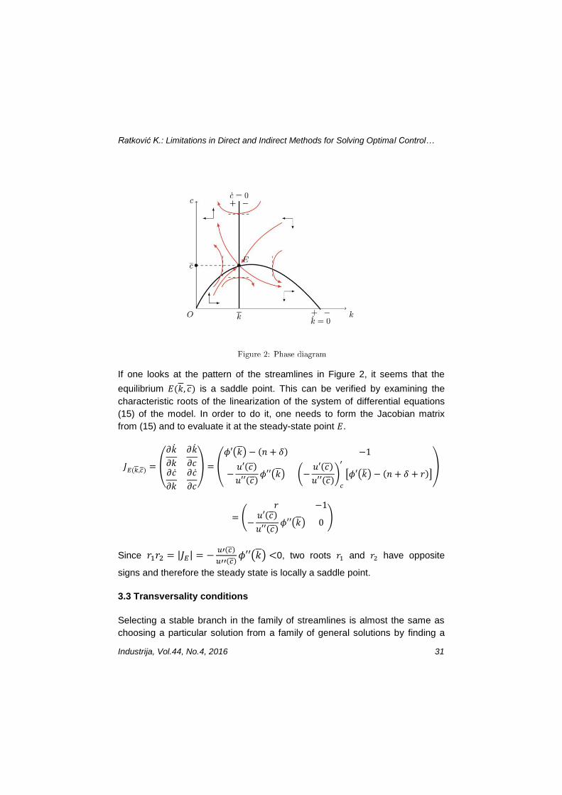
To construct the phase diagram, the curves �̇� = 0 and �̇� = 0 need to be plotted. Therefore, two equations are obtained:

𝑐 = 𝜙(𝑘) − (𝑛 + 𝛿)𝑘

𝜙′(𝑘) = 𝑛+ 𝛿+ 𝑟

The first curve is the difference between the curve of the function 𝜙(𝑘) and

the upward-sloping line (𝑛 + 𝛿)𝑘. The second curve requires that the slope of

the function 𝜙(𝑘) takes the value 𝑛 + 𝛿 + 𝑟. Since the function 𝜙(𝑘) is

monotonic and increasing, there is only one point in which this condition is

satisfied. Hence, the second curve must be plotted as a vertical straight line,

with horizontal intercept �̅�. The intersection of the two curves determines the

steady-state values of 𝑘 and 𝑐. These values, denoted by 𝑘 and 𝑐 are known

in literature as the modified-golden-rule values of capital-labor ratio and per-

capita consumption.



If one looks at the pattern of the streamlines in Figure 2, it seems that the

equilibrium 𝐸(𝑘, 𝑐) is a saddle point. This can be verified by examining the

characteristic roots of the linearization of the system of differential equations

(15) of the model. In order to do it, one needs to form the Jacobian matrix

from (15) and to evaluate it at the steady-state point 𝐸.

𝐽𝐸(𝑘,𝑐) =

(

𝜕�̇�

𝜕𝑘

𝜕�̇�

𝜕𝑐𝜕�̇�

𝜕𝑘

𝜕�̇�

𝜕𝑐)

= (

𝜙′(𝑘) − (𝑛 + 𝛿) −1

−𝑢′(𝑐)

𝑢′′(𝑐)𝜙′′(𝑘) (−

𝑢′(𝑐)

𝑢′′(𝑐))𝑐

′

[𝜙′(�̅�) − (𝑛 + 𝛿 + 𝑟)])

= (

𝑟 −1

−𝑢′(𝑐)

𝑢′′(𝑐)𝜙′′(𝑘) 0

)

Since 𝑟1𝑟2 = |𝐽𝐸| = −𝑢′(𝑐)

𝑢′′(𝑐)𝜙′′(𝑘) <0, two roots 𝑟1 and 𝑟2 have opposite

signs and therefore the steady state is locally a saddle point.

3.3 Transversality conditions

Selecting a stable branch in the family of streamlines is almost the same as

choosing a particular solution from a family of general solutions by finding a



particular constant. In order to do it, one will use the boundary conditions that

can be: either a specific initial 𝑐0 such that (𝑘0, 𝑐0 ) is on the stable branch or

an appropriate transversality condition. Since one has general functions and

therefore does not have quantitative solutions of differential equations, it is not

possible to describe a transversality condition. However, the phase-diagram

analysis can be used in order to verify that the steady-state solution satisfies

the expected transversality conditions. First transversality condition that the

steady-state solution is expected to satisfy is

lim𝑡→∞ 𝜆 = 0 (16)

Indeed, the solution path for 𝜆 is 𝜆∗ = 𝑢′(𝑐)𝑒−𝑟𝑡. It is clear that lim𝑡→∞ 𝑒−𝑟𝑡 =

0. On the other hand lim𝑡→∞ 𝑢′(𝑐) is finite, since it was assumed earlier that

lim𝑐→0 𝑢′(𝑐) = ∞ and in this case 𝑐∗ doos not tend to zero when 𝑡 → ∞.

Another transversality condition in the solution is

lim𝑡→∞ 𝐻 = 0 (17)

One knows from (6) that the solution path for 𝐻 is

𝐻∗ = 𝑢(𝑐∗)𝑒−𝑟𝑡 + 𝜆∗[𝜙(𝑘∗) − 𝑐∗ − (𝑛 + 𝛿)𝑘∗]

By (16), lim𝑡→∞ 𝜆∗ = 0 and lim𝑡→∞ 𝑢(𝑐

∗)𝑒−𝑟𝑡 = 0, since lim𝑡→∞ 𝑢(𝑐∗) is finite

and lim𝑡→∞ 𝑒−𝑟𝑡 = 0. The expression in the brackets 𝜙(𝑘∗)− 𝑐∗ − (𝑛 + 𝛿)𝑘∗

is exactly �̇� which is equal to zero in the steady state. Therefore, this

transversality condition is also satisfied.

3.4 Exogenous growth model with technological progress

The neoclassical growth model that has been discussed in the previous

section provides a steady state in which per-capita consumption 𝑐, stays

constant at 𝑐̅, with no further improvement in the average standard of living,

which comes from the static nature of the production function 𝑌 = 𝐹(𝐾, 𝐿).

Once technological progress is allowed, one can easily remove the cap on

per-capita consumption. There are three types of ``neutral’’ technological

progresses (the term neutral is because it leaves a certain economic variable

unaffected under certain condition): Hicks-neutral, Harrod-neutral and Solow-

neutral. The production function with Harrod-neutral technological progress is



𝑌 = 𝐹(𝐾, 𝐴(𝑡)𝐿) (18)

where 𝐹 is linearly homogenous in 𝐾 and 𝐴(𝑡)𝐿. Harrod-neutral technological

progress leaves the output-capital ratio (𝑌 𝐾⁄ ) unchanged at the same MPPK

(marginal product of capital). In exogenous growth models, Harrod neutrality

is frequently assumed since it is perfectly consistent with the notion of a

steady state. If we define efficiency labor 𝜂 = 𝐴𝐿, then the production

function (18) becomes

𝑌 = 𝐹(𝐾, 𝜂 ) (19)

If one now consider efficiency labor 𝜂 to be the relevant labor-input variable,

then (19) can be seen as a static production function. Using the homogeneity,

one can rewrite:

𝑦𝜂 = 𝜙(𝑘𝜂) 𝑤ℎ𝑒𝑟𝑒 𝑦𝜂 =𝑌

𝜂 𝑎𝑛𝑑 𝑘𝜂 =

𝐾

𝜂

This function is analogue to the production function 𝑦 = 𝜙(𝑘) in the neoclassical growth model. Following the same steps as at the beginning of this section, while maintaining all the assumptions on 𝜙, one can find the equation of motion for the new state variable 𝑘𝜂.

One obtains

𝑘𝜂̇ = 𝜙(𝑘𝜂)− 𝑐𝜂 − (𝑎 + 𝑛+ 𝛿)𝑘𝜂 (20)

𝑤ℎ𝑒𝑟𝑒 𝑐𝜂 =𝐶

𝜂, 𝑎 =

�̇�

𝐴 𝑎𝑛𝑑 𝑛 =

�̇�

𝐿 (21)

Hence, one has the following OCP:

𝑀𝑎𝑥𝑖𝑚𝑖𝑧𝑒 𝑈 = ∫ 𝑢 (𝑐𝜂(𝑡)) 𝑒−𝑟𝑡𝑑𝑡

+∞

0

𝑠𝑢𝑏𝑗𝑒𝑐𝑡 𝑡𝑜 𝑘�̇� = 𝜙(𝑘𝜂)− 𝑐𝜂 − (𝑎 + 𝑛+ 𝛿)𝑘𝜂

𝑘𝜂(0) = 𝑘𝜂0

𝑎𝑛𝑑 0 ≤ 𝑐𝜂 ≤ 𝜙(𝑘𝜂) (22)

The current-value Hamiltonian in the new problem is



𝐻𝑐′ = 𝑢(𝑐𝜂) + 𝑚′[𝜙(𝑘𝜂)− 𝑐𝜂 − (𝑎 + 𝑛+ 𝛿)𝑘𝜂] (23)

where 𝑚′ is the new current-value costate variable. By analogy, the maximum principle demands for the following conditions:

𝑚′ = 𝑢′(𝑐𝜂) (24)

𝑘𝜂̇ = 𝜙(𝑘𝜂)− 𝑐𝜂 − (𝑎 + 𝑛 + 𝛿)𝑘𝜂 (25)

𝑚′̇ = −𝑚′[𝜙′(𝑘𝜂)− (𝑎 + 𝑛+ 𝛿+ 𝑟)] (26)

By eliminating the variable 𝑚′, the following system of differential equations is obtained:

𝑘�̇� = 𝜙(𝑘𝜂)− 𝑐𝜂 − (𝑎 + 𝑛+ 𝛿)𝑘𝜂

𝑐�̇� = −𝑢′(𝑐𝜂)

𝑢′′(𝑐𝜂)[𝜙′(𝑘𝜂)− (𝑎 + 𝑛+ 𝛿+ 𝑟)]

The new phase diagram is constructed:

𝑘𝜂̇ = 0 ⇔ 𝑐𝜂 = 𝜙(𝑘𝜂)− (𝑎 + 𝑛+ 𝛿)𝑘𝜂

𝑐�̇� = 0 ⇔ 𝜙′(𝑘𝜂) =𝑎+ 𝑛+ 𝛿+ 𝑟

The new phase diagram is qualitatively the same as the one in the neoclassical growth model. However, there is one major difference which concerns the new steady state. Before, the per-capita consumption 𝑐 = 𝐶 𝐿⁄

was constant in a steady state. Now, one has that 𝑐𝜂 = 𝐶 𝜂⁄ = 𝐶 𝐴𝐿⁄ is

constant. Therefore, per-capita consumption 𝑐 = 𝑐𝜂𝐴 will rise over time, as

long as 𝐴 increases as a result of technological progress.

4. Endogenous growth model by Romer: indirect approach

Even though the exogenous technological progress remains quite simple, it

does not explain the origin of progress. In order to do it, it is necessary to

endogenize the technological progress. Endogenous growth models were

conceived as an attempt to overcome this theoretical nuance and to give a

consistent report to what causes economies to keep on growing (Romer

(1990), Lucas (1988), Uzawa (1965), Jones and Manuelli (1990)).



Knowledge in the Romer model (Romer, 1990), can be classified into two

components: human capital and technology. Human capital is person-specific

and it is a ``rival good˝ in the sense that its use by one firm excludes its use

by another. Technology is available to the public and it is a ``nonrival good˝ in

the sense that its use by one firm does not limit its use by others. Human

capital and technology are created by conscious action. In order to reduce the

number of state variables, human capital is assumed to be fixed and

inelastically supplied. Human capital will be denoted by 𝑆, and by 𝑆0 its fixed

total. Since 𝑆 can be used for the production of the final good 𝑌 or for the

improvement of technology 𝐴, one has:

𝑆0 = 𝑆𝑌 + 𝑆𝐴

On the other hand, technology 𝐴 is not fixed and can be created by engaging

human capital 𝑆𝐴 in research and applying the existing technology 𝐴:

�̇� = 𝜎𝑆𝐴𝐴 (27)

where 𝜎 denotes the research success parameter. One sees that �̇� 𝐴⁄ =

𝜎𝑆𝐴 > 0 if 𝜎 and 𝑆𝐴 are positive. Therefore, technology can grow without

bound. In the production of the final good 𝑌 variables 𝐿 and 𝐾 are inputs with

human capital 𝑆𝑌 and technology 𝐴. The production function is assumed to be

of Cobb-Douglas type:

𝑌 = 𝑆𝑦𝛼𝐿0𝛽𝐴�̅�1−𝛼−𝛽 (28)

where 𝐿0 denotes fixed and inelastically supplied amount of ordinary labor

and 𝑥 is the common level of use of ``design˝. Since the amount of capital

actually used will be

𝐾 = 𝛾𝐴�̅�

Therefore, the equation (28) becomes:

𝑌 = 𝑆𝑦𝛼𝐿0𝛽𝐴 (

𝐾

𝛾𝐴)1−𝛼−𝛽

= (𝑆𝑦𝐴)𝛼(𝐿0𝐴)

𝛽𝐾1−𝛼−𝛽𝛾𝛼+𝛽−1 (29)



One can see from the last expression that technology can be considered as

human capital increasing (𝑆𝑦𝐴) and as labor-increasing (𝐿0𝐴), but it is

detached from 𝐾. It is in a certain way endogenously characterized by Harrod-

neutrality.

Since the net investment is just the output that is not consumed, by

substituting:

�̇� = 𝑌 − 𝐶

= 𝛾𝛼+𝛽−1𝐴𝛼+𝛽(𝑆0 − 𝑆𝐴)𝛼𝐿0

𝛽𝐾1−𝛼−𝛽 − 𝐶 (30)

One can now consider an OCP with two state variables 𝐴 and 𝐾, and two

control variables 𝐶 and 𝑆𝐴, while the equations of motion are (27) and (30).

Assuming the constant elasticity of substitution (CES) utility function:

𝑢(𝐶) =𝐶1−𝜃

1 − 𝜃𝑤𝑖𝑡ℎ 0 < 𝜃 < 1

the following OCP can be defined:

𝑀𝑎𝑥𝑖𝑚𝑖𝑧𝑒 ∫𝐶1−𝜃

1 − 𝜃𝑒−𝜌𝑡𝑑𝑡

+∞

0

𝑠𝑢𝑏𝑗𝑒𝑐𝑡 𝑡𝑜 �̇� = 𝜎𝑆𝐴𝐴

�̇� = 𝛾𝛼+𝛽−1𝐴𝛼+𝛽(𝑆0 − 𝑆𝐴)𝛼𝐿0

𝛽𝐾1−𝛼−𝛽 − 𝐶

𝑎𝑛𝑑 𝐴(0) = 𝐴0 𝐾(0) = 𝐾0 (31)

In order to simplify the expression (30), one defines ∆= 𝛾𝛼+𝛽−1𝐴𝛼+𝛽(𝑆0 −

𝑆𝐴)𝛼𝐿0

𝛽𝐾1−𝛼−𝛽. Then the current-value Hamiltonian is

𝐻𝑐 =𝐶1−𝜃

1−𝜃+ 𝜆𝐴(𝜎𝑆𝐴𝐴)+ 𝜆𝐾(∆ − 𝐶) (32)

where 𝜆𝐴 and 𝜆𝐾 denote the shadow prices of 𝐴 and 𝐾, respectively. By the

necessary condition for the existence of a maximum

𝜕𝐻𝑐

𝜕𝐶= 𝐶−𝜃 − 𝜆𝐾 = 0 ⇔ 𝜆𝐾 = 𝐶

−𝜃 (33)



𝜕𝐻𝑐

𝜕𝑆𝐴= 𝜆𝐴𝜎𝐴 − 𝜆𝐾𝛼(𝑆0 − 𝑆𝐴)

−1∆= 0 ⇔ ∆=𝜆𝐴𝜎𝐴

𝜆𝐾𝛼(𝑆0 − 𝑆𝐴) (34)

The maximum principle demands in addition to the two equations of motion �̇�

and �̇�, two equations of motion for the costate variables:

𝜆𝐴̇ = −𝜕𝐻𝑐𝜕𝐴

+ 𝜌𝜆𝐴 = −𝜆𝐴𝜎𝑆𝐴 − 𝜆𝐾(𝛼 + 𝛽)𝐴−1∆ + 𝜌𝜆𝐴

𝜆�̇� = −𝜕𝐻𝑐

𝜕𝐾+ 𝜌𝜆𝐾 = −𝜆𝐾(1 − 𝛼 − 𝛽)𝐾

−1∆ + 𝜌𝜆𝐾 (35)

Having four differential equations, it is not possible to construct a phase

diagram and it is difficult to solve the system explicitly. However, some

questions can be answered in the steady state. Variables 𝑌, 𝐾, 𝐴 and 𝐶 grow

at the same rate. Therefore, by (27), one has:

�̇�

𝐴=�̇�

𝑌=�̇�

𝐾=�̇�

𝐶= 𝜎𝑆𝐴 (36)

Since the growth rate should be expressed only in terms of parameters, it is

necessary to find the expression for 𝑆𝐴. Indeed, the expressions for �̇�𝐴 𝜆𝐴⁄ and

�̇�𝐾 𝜆𝐾⁄ can be found from (35) and then use the fact that in the steady

state: �̇�𝐴 𝜆𝐴⁄ = �̇�𝐾 𝜆𝐾⁄ . Therefore, 𝑆𝐴 reaches in the steady state the constant

value:

𝑆𝐴 =𝜎(𝛼+𝛽)𝑆0−𝛼𝜌

𝜎(𝛼𝜃+𝛽) (37)

The growth rate is

�̇�

𝐴=�̇�

𝑌=�̇�

𝐾=�̇�

𝐶=𝜎(𝛼+𝛽)𝑆0−𝛼𝜌

𝛼𝜃+𝛽 (38)

The expression (38) tells us how the various parameters affect the growth

rate. One can see that the research success parameter 𝜎 and the human

capital 𝑆0 have a positive effect on the growth rate, and that the discount rate

𝜌 has the negative effect.



5. Endogenous growth model by Lucas and Uzawa: direct

approach

The Uzawa-Lucas model introduces human capital ℎ, as another productive

input of the economy that is produced by a different technology than that of

physical capital 𝐾. Also, labor 𝐿 can either be employed in final output

production, 𝜇, with the rest 1 − 𝜇 that is dedicated to formal education. This

model exposes steady-state growth, in the sense that consumption and

capital (physical and human) is unbounded. The introduction of human capital

and specialized labor adds another state and control variable respectively to

the system, and adds complexity as well. In fact, the transition process of this

model is still vague, since the indirect methods for solving the underlying OCP

give origin to rigid ordinary differential equations, which gives an extra

difficulty, as Trimborn et al. (2004) noticed. This model uses the framework

specified in Section 3. Households try to maximize their utility by consuming

according to a standard CES function 𝑢(𝐶). One has the following production

function:

𝑌 = 𝐴𝐾𝛼(𝑢ℎ𝐿)1−𝛼 (39)

Physical capital 𝐾 and human capital ℎ follow the laws of motion:

�̇� = 𝑌 − 𝐶 − 𝛿𝐾 (40)

ℎ̇ = 𝐵(1 − 𝑢)ℎ − 𝛿ℎℎ (41)

where 𝐵 is a constant reflecting productivity of quality adjusted effort in

education and 𝛿ℎ (0 ≤ 𝛿ℎ < 𝐵) is the depreciation rate of human capital,

which is set 𝛿ℎ = 0.

Using per-capita variables 𝑘, 𝑦 and 𝑐 and without population growth (𝑛 = 0),

the following OCP can be defined:

𝑀𝑎𝑥𝑖𝑚𝑖𝑧𝑒 ∫𝐶1−𝜃


+∞

0

𝑠𝑢𝑏𝑗𝑒𝑐𝑡 𝑡𝑜 �̇� = 𝐴𝐾𝛼(𝑢ℎ)1−𝛼 − c − δk

ℎ̇ = 𝐵(1 − 𝑢)ℎ



𝑎𝑛𝑑 𝑘(0) = 𝑘0 ℎ(0) = ℎ0 (42)

The outline that will be presented results from the work of Fontes (2001) and

follows the approach used by Lopes et al. (2013). The first step is to

transcribe the infinite horizon problem into a finite dimensional problem. The

second is to prove that this nonlinear programming problem (NLP) is

equivalent to the original one. Finally, an advanced NLP solver could be used

in order to find the optimal trajectories. As opposed to indirect methods, the

OCP is first discretized and then optimized.

The first step is to present the following theorem that enables us to discretize

the infinite horizon problem.

Theorem 1. (Lopes et al., 2013)

Consider the following generic optimal control problem:

𝑃∞: 𝑀𝑖𝑛𝑖𝑚𝑖𝑧𝑒 ∫ 𝐿(𝑥(𝑡), 𝑢(𝑡))𝑑𝑡+∞

0

𝑠𝑢𝑏𝑗𝑒𝑐𝑡 𝑡𝑜 �̇� = 𝑓(𝑥, 𝑢)

𝑥(0) = 𝑥0

𝑎𝑛𝑑 𝑥(𝑡) ∈ 𝛤(𝑡) 𝑢(𝑡) ∈ 𝛺(𝑡) (43)

where we assume that there is a finite solution. Furthermore, we assume that

after some time 𝑇, the state is within some invariant set 𝑆 ( 𝑖. 𝑒. 𝑥(𝑡) ∈ 𝑆, 𝑆 ⊂

𝛤(𝑡), ∀𝑡 ≥ 𝑇) for which the problem still has a finite solution.

Then there exists a terminal cost function W, such that the optimal control

problem is equivalent to the finite horizon problem:

𝑃𝑇: 𝑀𝑖𝑛𝑖𝑚𝑖𝑧𝑒 ∫ 𝐿(𝑥(𝑡), 𝑢(𝑡))𝑑𝑡 +𝑊(𝑥(𝑡))𝑇

0

𝑠𝑢𝑏𝑗𝑒𝑐𝑡 𝑡𝑜 �̇� = 𝑓(𝑥, 𝑢)

𝑥(0) = 𝑥0

𝑎𝑛𝑑 𝑥(𝑡) ∈ 𝛤(𝑡) 𝑢(𝑡) ∈ 𝛺(𝑡) 𝑥(𝑇) ∈ 𝑆 (44)



Proof. Consider problem 𝑃∞ with 𝛤(𝑡) = 𝑆 for all 𝑡 ≥ 𝑇. Then the value for 𝑃∞

is

𝑉(0, 𝑥0) = 𝑚𝑖𝑛 {∫ 𝐿(𝑥, 𝑢(𝑡))𝑑𝑡 + 𝑉(𝑡, 𝑥(𝑡))𝑇

0

}

Now, one can define

𝑊(𝑥(𝑡)) = 𝑉(𝑇, 𝑥(𝑇)) = min𝑥∈𝑆

{∫ 𝐿(𝑥, 𝑢)𝑑𝑡+∞

𝑇

}

and discretize 𝑃∞ into 𝑃𝑇.

Theorem 1 can be applied only when the set 𝑆 is such that the

characterization of the solution to the problem is possible

𝑊(𝑥(𝑡)) = min𝑥∈𝑆

{∫ 𝐿(𝑥(𝑡), 𝑢(𝑡))𝑑𝑡+∞

𝑇

}

and therefore 𝑊(𝑥) can explicitly be computed for any 𝑥 ∈ 𝑆.

The following procedure is applied:

1. Transcription of the infinite-horizon problem into an equivalent finite-horizon

problem by applying Theorem 1;

2. Adding the necessary boundary conditions that ensure that the set 𝑆 is

invariant (and so 𝑊(𝑥) exists for any 𝑥 ∈ 𝑆);

3. Using a NLP solver to determine the trajectories of the control and state

variables.

It is known that in balanced growth we have:

𝑐̇

𝑐=�̇�

𝑦=�̇�

𝑘=ℎ̇

ℎ= 𝛾 (45)

If one defines

𝑤 =𝑘

ℎ 𝑎𝑛𝑑 𝜒 =

𝑐

𝑘



and it is known that in the steady state, for 𝑡 ≥ 𝑇, one has �̇� = 0 and �̇� = 0

(Barro et al., 2003). Define the control functions

𝑐(𝑡) = 𝜒𝑘(𝑡) 𝑎𝑛𝑑 𝑘(𝑡) = 𝑤ℎ(𝑡) (46)

such that 𝜒 and 𝑤 are equal to a given positive constant.

One has

�̇�

𝑘= 𝐴𝑘𝛼−1(𝑢ℎ)1−𝛼 − 𝜒 − δ = (

𝑢ℎ

𝐴𝑘)1−𝛼

− 𝜒 − δ = (𝑢

𝐴𝑤)1−𝛼

− 𝜒 − δ

but also

�̇�

𝑘=𝑤ℎ̇

𝑤ℎ= 𝐵(1 − 𝑢) = 𝛾

Therefore, equation (46) is obtained with 𝑢(𝑡) = 𝑢 constant and one has:

(𝑢

𝐴𝑤)1−𝛼

− 𝜒 − δ = B(1 − 𝑢)

Moreover, one has

�̇�

𝑐=�̇�

𝑘=ℎ̇

ℎ= 𝐵(1 − 𝑢)

which implies that �̇� = 𝛾𝑐 in a balanced growth path. At the time 𝑡 = 𝑇

consumption 𝑐 will continue to grow at rate 𝛾

𝑐(𝑡) = 𝑐(𝑇)𝑒𝛾(𝑡−𝑇), 𝑡 ∈ [𝑇, +∞)

which enables us to compute 𝑊. Utility will be bounded as 𝜌 > 𝛾(1 − 𝜃) so

that 𝑈(∙,∞) = 0. Then the boundary cost is given by

𝑊 = −∫(𝑐(𝑇)𝑒𝛾(𝑡−𝑇))

1−𝜃


+∞

𝑇

Finding the integral

𝑊 = −𝑒𝛾(1−𝜃)−𝜌

𝜌−𝛾(1−𝜃) ∙ (𝑐(𝑇)𝑒−𝛾𝑇)

1−𝜃

1−𝜃 (47)



The boundary condition will be

𝑆 = {(𝑘, ℎ) ∈ 𝑅2 ∶ �̇�

𝑘=ℎ̇

ℎ= 0} 𝑠. 𝑡. 𝑘(𝑇), ℎ(𝑇) ∈ 𝑆 (48)

The system defined by (42) together with the boundary cost 𝑊 (47) and the

boundary condition 𝑆 (48) can now be solved numerically using a NLP solver.

Lopes et al. (2013) use the software ICLOCS that solves OCP with general

path and boundary constraints and free or fixed final time (actually this

software uses another software called IPOPT to solve the transformed NLP

problem).

More generally, there are numerous and powerful softwares (NLP solvers)

that are used to find numerical solutions of OCP. Some of them can be

named: SNOPT, ICLOCS, DIRCOL, SOCS, OTIS, GESOP/ASTOS, DITAN

and PyGMO/PyKEP.

These numerical results should be evaluated in order to measure the

accuracy of numerical methods. There are different studies of this procedure

of evaluation (Aruoba et al. (2006), Ambler and Pelgrin (2006) and Heer and

Maubner (2008)).

It is important to notice, that using the direct approach, optimal trajectories can be determined numerically and without demanding the linearization of the differential equations. This can avoid some problems that can occur by a change of base or any other manipulation. It also allows the study of the transition process when it is not necessary for the system to depart from a steady state or to be at a steady state. Furthermore, it is a powerful tool to study some complex phenomena like anticipated or multiple, sequential shocks. Mainly, to study such shocks using indirect methods, authors like Trimborn (2007) suggest a reformulation of the optimization problem, which

consists in decomposing the functional form of the objective function from 𝑓(1) to 𝑓(2) and the state equations from 𝑔(1) to 𝑔(2) at time �̃� when shock occurs. The necessary optimality conditions would have to be augmented with the conditions derived from the interior boundary condition. Moreover, the adjoint variable functions introduced by the Maximum Principle have to satisfy the condition of continuity, also known as the Weierstrass-Erdmann corner condition. Using the direct approach, it is not required to reformulate the model. Indeed, one does not need to determine or even know any necessary optimality conditions, which can be particularly useful for problems whose adjoint functions are hard to find.



Conclusion

The indirect and direct methods for solving OCP can be used in both,

exogenous and endogenous models of growth. The indirect methods for

solving OCP provide better insight into the core of the optimization process in

the theory of economic growth, but are sometimes very difficult to solve. In

particular, the linearization of the dynamic system of differential equations can

become very difficult. As a result, simplicity of the model is often required, so

that the analytical solutions could be found. On the other side, direct methods

seem to be faster and more efficient, even if they do not follow the logical,

standard procedure of optimization. Moreover, they allow the study of the

transitional dynamics of models that are not at their steady-state, and also to

study expected and unexpected shocks. However, the process of

discretization (transcription of the infinite horizon problem into a finite

dimensional problem) of the OCP into a NLP, can become quite artificial and

sometimes hard to prove. In general, the choice of a method for solving OCP

will mainly depend on two major points: the importance of the insight of the

optimization process and the complexity of the given OCP.

References

Acemoglu, D. (2007). Introduction to modern economic growth (Levine's Bibliography).

UCLA Department of Economics. Aghion, P., & Howitt, P. (1998). Endogenous growth theories. Cambridge, MA: MIT

Press. Arrow, K.J. (1968). Applications of control theory to economic growth. (pp. 85-119).

Providence: American Mathematical Society. Arrow, K.J., & Kurz, M. (1970). Public investment, the rate of return and optimal fiscal

policy. Baltimore - London: Johns Hopkins Press. Aseev, S. (2009). Infinite-horizon optimal control with applications in growth theory.

lecture notes. Atolia, M., Chatterjee, S., & Turnovsky, S.J. (2008). How Misleading is Linearization?,

Evaluating the Dynamics of the Neoclassical Growth Model. Florida: Department of Economics, State University. Working Papers.

Barro, R.J., & Sala-i, M.X. (2003). Economic Growth, 2nd ed. The MIT Press. Vol. 1. Bellman, R. (1957). Dynamic programming, 1st ed. Princeton, NJ, USA: Princeton

University Press. Betts, J.T. (2001). Practical methods for optimal control using nonlinear programming.

Philadelphia: SIAM Press - Princeton University Press.



Brunner, M., & Strulik, H. (2002). Solution of perfect foresight saddlepoint problems: A simple method and applications. Journal of Economic Dynamics and Control, 26(5), 737-753.

Cass, D. (1965). Optimum growth in an aggregative model of capital accumulation. Review of Economic Studies, 32(3), 233-240.

Chiang, A.C. (1992). Elements of dynamic optimization. New York: McGraw-Hill.. Dixit, A.K. (1990). Optimization in Economic Theory. Oxford University Press. Dorfman, R. (1969). An Economic Interpretation of Optimal Control Theory. American

Economic Review, 59(5), 817-831. Fabbri, G., & Gozzi, F. (2008). Solving optimal growth models with vintage capital: The

dynamic programming approach. Journal of Economic Theory, 143(1), 331-373. Fontes, F. (2001). A general framework to design stabilizing nonlinear model predictive

controllers. Systems & Control Letters, Gill, P.E., Murray, W., & Saunders, M.A. (2005). SNOPT: An SQP algorithm for large-

scale constrained optimization. SIAM Rev., 47, 99-131. Gill, P.E., Murray, W., Saunders, M.A., & Wong, E. (2015). User's guide for SNOPT 7.

5: Software for large-scale nonlinear programming. Center for Computational Mathematics Report, 15-3, CCoM, La Jolla, CA: Department of Mathematics, University of California, San Diego.

Inada, K.I. (1963). On a two-sector model of economic growth: Comments and a generalization. Review of Economic Studies, 30(2), 119-127.

Intriligator, M.D. (1971). Mathematical optimization and economic theory. Englewood Clis, N. J.: Prentice Hall..

Judd, K.L. (1992). Projection methods for solving aggregate growth models. Journal of Economic Theory, 58(2), 410-452.

Judd, K.L. (1998). Numerical Methods in Economics. The MIT Press. Vol. 1. Kamien, M.I., & Schwartz, N.L. (1991). Dynamic Optimization: The Calculus of

Variations and Optimal Control in Economics and Management, 2nd ed. Elsevier

Science. Koopmans, T. (1963). On the concept of optimal economic growth. Cowles Foundation

Discussion Papers, 163, Cowles Foundation for Research in Economics, Yale University.

Ljungqvist, L., & Sargent, T.J. (2012). Recursive Macroeconomic Theory, 3rd ed. The MIT Press. Vol. 1.

Lopes, M.A., Fontes, F.A.C.C., & Fontes, D.A.C.C. (2013). Optimal Control of Infinite-Horizon Growth Models-A direct approach. FEP Working Papers, Universidade do Porto, Faculdade de Economia do Porto.

Lucas, R.J. (1988). On the mechanics of economic development. Journal of Monetary Economics, 22(1), 3-42.

Mercenier, J., & Michel, P. (1994). Discrete-Time Finite Horizon Appromixation of Infinite Horizon Optimization Problems with Steady-State Invariance. Econometrica, 62(3), 635-656.

Mulligan, C.B., & Sala-i Martin, X. (1991). A Note on the Time-Elimination Method For Solving Recursive Dynamic Economic Models. NBER Technical Working Papers, 0116, National Bureau of Economic Research, Inc..

Pontryagin, L.S., Boltyanskii, V.G., Gamkrelidze, R.V., & Mishchenko, E.F. (1962). The mathematical theory of optimal processes. New York: Interscience.

Ramsey, F. (1928). A mathematical theory of saving. Economic Journal, 38, 543-559.



Rao, A.V. (2009). A survey of numerical methods for optimal control. Advances in the Astronautical Sciences, 135(1), 497-528.

Romer, P.M. (1990). Endogenous Technological Change. Journal of Political Economy, 98(5), 71-102.

Romer, P.M. (1994). The origins of endogenous growth. The Journal of Economic Perspectives, 8(1), 3-22.

Sargent, R. (2000). Optimal control. Journal of Computational and Applied Mathematics, 124(12), 361-371.

Solow, R. (1956). A contribution to the theory of economic growth. The Quarterly Journal of Economics, 70(1), 65-94.

Stokey, N., Lucas, R.E., & Prescott, E.C. (1989). Recursive methods in economic dynamics. Cambridge, Mass: Harvard University Press.

Trimborn, T., Koch, K.J., & Steger, T.M. (2004). Multi-dimensional transitional dynamics: A simple numerical procedure. CER-ETH Economics working paper series,

Uzawa, H. (1965). Optimum technical change in an aggregative model of economic growth. International Economic Review, 6(1), 18-31.

von Stryk, O., & Bulirsch, R. (1992). Direct and indirect methods for trajectory optimization. Ann. Oper. Res., 37(1-4), 357-373.

Wolman, A.L., & Couper, E.A. (2003). Potential consequences of linear approximation in economics. Economic Quarterly, 51-67.

limitations in direct and indirect methods for solving ...apstrakt: fokus ovog članka je na...

Documents