limit theorems for persistence diagrams

The Annals of Applied Probability2018, Vol. 28, No. 5, 2740–2780https://doi.org/10.1214/17-AAP1371© Institute of Mathematical Statistics, 2018

LIMIT THEOREMS FOR PERSISTENCE DIAGRAMS1

BY YASUAKI HIRAOKA∗, TOMOYUKI SHIRAI†,2 AND KHANH DUY TRINH†,3

Tohoku University∗ and Kyushu University†

The persistent homology of a stationary point process on RN is studiedin this paper. As a generalization of continuum percolation theory, we studyhigher dimensional topological features of the point process such as loops,cavities, etc. in a multiscale way. The key ingredient is the persistence dia-gram, which is an expression of the persistent homology. We prove the stronglaw of large numbers for persistence diagrams as the window size tends to in-finity and give a sufficient condition for the support of the limiting persistencediagram to coincide with the geometrically realizable region. We also discussa central limit theorem for persistent Betti numbers.

1. Introduction.

1.1. Background. The prototype of this work dates back to the random geo-metric graphs. In those original settings, a set V of points is randomly scattered ina space according to some probability distribution, and a graph with the verticesV is constructed by assigning edges whose distances are less than a certain thresh-old value r ≥ 0. Then some characteristic features in the graph such as connectedcomponents and loops are broadly and thoroughly studied (see, e.g., [30]). Further-more, the random geometric graphs provide mathematical models for applicationssuch as mobile wireless networks [25, 27], epidemics [34], and so on.

Recently, the concept of random topology has emerged and rapidly grown asa higher dimensional generalization of random graphs [3, 23]. One of the simplemodels studied in random topology is a simplicial complex, which is given by acollection of subsets closed under inclusion. Obviously, a graph is regarded as aone-dimensional simplicial complex consisting of singletons as vertices and dou-bletons as edges.

In geometric settings, a simplicial complex is built over randomly distributedpoints in a space by a certain rule respecting the nearness of multiple points, likerandom geometric graphs. Two standard simplicial complex models constructed

Received December 2016; revised August 2017.1Supported in part by JST CREST Mathematics (15656429).2Supported in part by JSPS Grant-in-Aid (JP26610025, JP26287019, JP16H06338).3Supported in part by JSPS Grant-in-Aid for Young Scientists (B) (JP16K17616).MSC2010 subject classifications. Primary 60K35, 60B10; secondary 55N20.Key words and phrases. Point process, persistence diagram, persistent Betti number, random

topology.

2740

http://www.imstat.org/aap/

https://doi.org/10.1214/17-AAP1371

http://www.imstat.org

http://www.ams.org/mathscinet/msc/msc2010.html

LIMIT THEOREMS FOR PERSISTENCE DIAGRAMS 2741

from the points are Cech complexes and Rips complexes, which are also deter-mined by a threshold value r measuring the nearness of points. Then, in such anextended geometric object, it is natural to study higher dimensional topologicalfeatures such as cavities (2 dim.) and more general q-dimensional holes, beyondconnected components (0 dim.) and loops (1 dim.).

In algebraic topology, q-dimensional holes are usually characterized by usingthe so-called homology. Here, the qth homology of a simplicial complex is givenby a vector space and its dimension is called the Betti number which counts thenumber of q-dimensional holes. Hence, in the setting of random simplicial com-plexes, the Betti numbers become random variables through a random point con-figuration, and studying the asymptotic behaviors of the randomized Betti numbersis a significant problem for understanding global topological structures embeddedin the random simplicial complexes (e.g., [22, 29, 37–39]).

On the other hand, another type of generalizations has been recently attract-ing much attention in applied topology. In that setting, we are interested in howpersistent the holes are for changing the threshold parameter r ∈ R. Namely, wedeal with one parameter filtration of simplicial complexes obtained by increas-ing the parameter r and characterize robust or noisy holes in that filtration. Thepersistent homology [10, 40] is a tool invented for this purpose, and especially,its expression called persistence diagram is now applied to a wide variety of ap-plied areas (see, e.g., [4, 11, 16, 28, 35]). From this point of view, there have beensome works on a functional of persistence diagram, called lifetime sum or totalpersistence, for random complexes (that are not geometric in the sense above)such as Linial–Meshulam processes and random cubical complexes (e.g., [17–19]).

Therefore, it is natural to further extend the results on random geometric sim-plicial complexes to this generality, and the purpose of this paper is to show sev-eral of these extensions. In particular, we are interested in asymptotic behaviorsof persistence diagrams themselves defined on stationary point processes. Thesesubjects are mathematically meaningful in their own right, but are also interest-ing for practical applications. For example, the paper [16] studies topological andgeometric structures of atomic configurations in glass materials by comparing per-sistence diagrams with those of disordered states. By regarding atomic configu-rations in disordered states as random point processes, further understanding ofthose persistence diagrams will be useful for characterizing geometry and topol-ogy of glass materials, which is one of the important research topics in currentphysics.

1.2. Prior work. Let � be a stationary point process on RN with all finitemoments, that is,

(1.1) E[�(A)k

]< ∞ for all bounded Borel sets A and any k = 1,2, . . . .

2742 Y. HIRAOKA, T. SHIRAI AND K. D. TRINH

Here, �(A) denotes the number of points in A. For simplicity, we always assumethat � is simple, that is,

P(�({x})≤ 1 for every x ∈ RN )= 1.

We denote by ��Lthe restriction of � on �L = [−L

2 , L2 )N .

Let C(��L, r) be the Cech complex built over the points ��L

with parameterr > 0 (see Section 2.1 for the definition). The 0th Betti number β0(C(��L

, r)) forPoisson point processes, which is closely related to the binomial processes, hasbeen studied in an extensive literature (cf. [30]) from various points of view suchas the geometric percolation theory and computational geometry. Recently, thelimiting behaviors of higher Betti numbers βq(C(��L

, r)) (q = 1,2, . . . ,N − 1)over general stationary point processes have also been widely investigated [38,39]. Among them, we here restate the most related results.

THEOREM 1.1 ([39], Lemma 3.3 and Theorem 3.5). Assume that � is a sta-tionary point process on RN having all finite moments. Then, for each 0 ≤ q ≤N − 1, there exists a constant βr

q ≥ 0 such that

E[βq(C(��L, r))]

LN→ βr

q as L → ∞.

In addition, if � is ergodic, then

βq(C(��L, r))

LN→ βr

q almost surely as L → ∞.

THEOREM 1.2 ([39], Theorem 4.7). Assume that � is a homogeneous Poissonpoint process on RN with unit intensity. Then, for each 0 ≤ q ≤ N − 1, there existsa constant σ 2

r > 0 such that

βq(C(��L, r)) −E[βq(C(��L

, r))]LN/2

d→ N(0, σ 2

r

)as L → ∞.

Here, N (μ,σ 2) denotes the normal distribution with mean μ and variance σ 2,

andd→ denotes the convergence in distribution of random variables.

The purpose of this paper is to extend Theorem 1.1 to the setting on persistencediagrams and Theorem 1.2 to persistent Betti numbers.

1.3. Main results. In this paper, we study the following simplicial complexmodel for the point process � which is a generalization of the Cech complex andthe Rips complex.

Let F (RN) be the collection of all finite (nonempty) subsets in RN . We canidentify F (RN) with the set

⊔∞k=1(R

N)k/ ∼, where ∼ is the equivalence rela-tion induced by permutations of coordinates. For a function f on F (RN), there


exists a permutation invariant function fk on (RN)k for each k ≥ 1 such thatf ({x1, . . . , xk}) = fk(x1, . . . , xk). We say that f is measurable if so is fk on (RN)k

for each k ≥ 1.Let κ : F (RN) → [0,∞] be a measurable function satisfying:

(K1) 0 ≤ κ(σ ) ≤ κ(τ), if σ is a subset of τ ;(K2) κ is translation invariant, that is, κ(σ + x) = κ(σ ) for any x ∈ RN , where

σ + x := {y + x : y ∈ σ };(K3) there is an increasing function ρ : [0,∞] → [0,∞] with ρ(t) < ∞ for

t < ∞ such that

‖x − y‖ ≤ ρ(κ({x, y})),

where ‖x‖ denotes the Euclidean norm in RN .

Without loss of generality, we can assume κ({x}) = 0 because of the translationinvariance.

Given such a function κ , we construct a filtration K() = {K(, t) : 0 ≤ t <

∞} of simplicial complexes from a finite point configuration ∈ F (RN) by

K(, t) = {σ ⊂ : κ(σ ) ≤ t

},(1.2)

that is, κ(σ ) is the birth time of a simplex σ in the filtration K(). Although we donot explicitly show the dependence on κ in the notation K() because the functionκ is fixed in the paper, we here call it the κ-filtration over .

EXAMPLE 1.3. Two important examples of κ which we have in mind are

κC

({x0, x1, . . . , xq})= infw∈RN

max0≤i≤q

‖xi − w‖,(1.3)

κR

({x0, x1, . . . , xq})= max0≤i<j≤q

‖xi − xj‖2

,(1.4)

which define the Cech filtration C(�) = {C(�, t)}t≥0 and the Rips filtrationR(�) = {R(�, t)}t≥0, respectively. Both κ’s satisfy Assumption (K3) withρ(t) = 2t . See also Section 2.1 for these filtrations.

For Theorem 1.9 below, we also remark that both κC and κR are 1-Lipshitzcontinuous on F (RN) with respect to the Hausdorff distance dH . See AppendixC for the definition of dH .

For the filtration K(), we denote its qth persistence diagram by

Dq() = {(bi, di) ∈ : i = 1, . . . , nq

},

which is given by a multiset on = {(x, y) ∈ R2 : 0 ≤ x < y ≤ ∞} determined

from the unique decomposition of the persistent homology (see (2.2) for the def-inition). The pair (bi, di) indicates the persistence of the ith homology class, that


is, it appears at bi and disappears at di , and di = ∞ means that the ith homologyclass persists forever.

In this paper, we deal with the persistence diagram Dq() as the counting mea-sure

ξq() = ∑(bi ,di )∈Dq()

δ(bi ,di ),

rather than as a multiset, where δ(x,y) is the Dirac measure at (x, y) ∈ R2.

For each L > 0, we define a random filtration built over the points ��Land de-

note it by K(��L) = {K(��L

, t)}t≥0. We write ξq,L for the point process ξq(��L)

and E[ξq,L] for its mean measure (see Section 3 for the precise definition of meanmeasure).

EXAMPLE 1.4. The top three panels in Figure 1 show point processes withnegative (Ginibre), zero (Poisson) and positive (Poisson cluster) correlations, re-spectively (see [2] for more examples and correlation properties of point processesincluding the above). All point processes consist of 1,000,000 points with the den-sity 1/2π , and only restricted areas of them are visualized. The bottom shows thecorresponding normalized persistence diagrams ξ1,L/L2 of the Cech filtrations ap-plied to the above, respectively.

FIG. 1. Top: Point processes with negative (Ginibre), zero (Poisson), and positive (Poisson clus-ter) correlations. In these three point processes, the number of points and the density are set to be1,000,000 and 1/2π , respectively. Bottom: The normalized persistence diagrams ξ1,L/L2 of theabove.


One of the main results in this paper is as follows.

THEOREM 1.5. Assume that � is a stationary point process on RN having allfinite moments. Then, for each q ≥ 0, there exists a unique Radon measure νq on such that

(1.5)1

LNE[ξq,L] v→ νq as L → ∞.

Here,v→ denotes the vague convergence of measures on . In addition, if � is

ergodic, then almost surely,

(1.6)1

LNξq,L

v→ νq as L → ∞.

We call the limiting Radon measure νq the qth persistence diagram of a station-ary ergodic point process �. In nonergodic case, by using the ergodic decomposi-tion (cf. [14]), the right-hand side in (1.6) is replaced by the random measure νq,ω

which is measurable with respect to the translation invariant σ -field I defined inSection 3.

REMARK 1.6. The set is topologically the same as the triangle{(x, y) ∈ R2 : 0 ≤ x < y ≤ 1

}with open boundary ∂ = {(x, x) ∈ R2 : 0 ≤ x ≤ 1}. Although we do not con-sider the mass on ∂, intuitively speaking, the (virtual) mass on ∂ comes fromconfigurations of special forms such as three vertices of a right triangle. With thevague convergence, we do not see the mass escaping towards the boundary ∂ inthe limit L → ∞. In applications, the mass appearing near the boundary is con-sidered to be fragile under perturbation while the one away from the boundary isconsidered to be robust.

The limiting measure νq may be trivial. Indeed, for Cech complexes, νq = 0 forq ≥ N . This is just because there is no configuration in RN that realizes the qthhomology class for q ≥ N . In order to characterize the support of νq , we introducethe notion of realizability of a point in a persistence diagram.

DEFINITION 1.7. We say that a point (b, d) ∈ is realizable by ∈ F (RN)

in the qth persistent homology if (b, d) is contained in the qth persistence diagramof the κ-filtration over , that is, ξq()({(b, d)}) ≥ 1. If such exists for (b, d),we call (b, d) a realizable point. We denote by Rq = Rq(κ) the set of all realizablepoints in the qth persistent homology of the κ-filtration.


EXAMPLE 1.8. For α > 0 and σ ∈ F (RN), we define ασ ∈ F (RN) by ασ ={αx ∈ RN : x ∈ σ }. It is easy to see that if κ is homogeneous in the sense thatκ(ασ) = ακ(σ ) for every α > 0 and σ ∈ F (RN), then Rq(κ) forms a cone in .Since both κC and κR given in Example 1.3 are homogeneous, we can see thatRq(κC) and Rq(κR) are cones for every q ≥ 0. In particular, for Cech complexes,we have

Rq(κC) =

⎧⎪⎪⎨⎪⎪⎩{0} × (0,∞] if q = 0,{(b, d) : 0 < b < d < ∞}

if q = 1,2, . . . ,N − 1,

∅ if q = N,N + 1, . . . .

(1.7)

The sketch of the proof is given at the end of Section 2.2.

It is clear that suppνq ⊂ Rq(κ). Indeed, if x /∈ Rq(κ), there exists ε > 0 suchthat ξq,L(Bε(x)) = 0, where Bε(x) is the open ε-neighborhood of x. It followsfrom the vague convergence (1.5) that νq(Bε(x)) = 0. Therefore, x /∈ suppνq . InTheorem 4.7, we give sufficient conditions for a point in Rq(κ) to be in the supportof νq . The following result, as a consequence of that general theorem, states thatsuppνq coincides with Rq(κ) under conditions that κ is Lipschitz continuous andall local densities of the point process � are almost surely positive with respect tothe Lebesgue measures.

THEOREM 1.9. Let � be a stationary point process on RN and � its prob-ability distribution. Assume that for every compact set � ⊂ RN , the restriction�|� on � is absolutely continuous with respect to �|� and the Radon–Nikodymdensity d�|�/d�|� is strictly positive �|�-almost surely, where � is the distri-bution of a homogeneous Poisson point process on RN . In addition, assume thatκ on F (RN) is Lipschitz continuous with respect to the Hausdorff distance. Thensuppνq = Rq(κ) for every q ≥ 0.

EXAMPLE 1.10. All finite configurations are allowed to appear in a point pro-cess if the positivity assumption in Theorem 1.9 holds. There are many “natural”stationary point processes satisfying the assumption. Homogeneous Poisson pointprocesses, a certain class of Gibbs point processes, Ginibre point processes andthe zeros of the Gaussian entire function X(z) =∑∞

n=0(n!)−1/2anzn with {an}n≥0

being i.i.d. complex standard Gaussian random variables, etc. are such exam-ples. Thus if κ is Lipschitz continuous with respect to the Hausdorff distance,then suppνq = Rq(κ) for such point processes. In particular, for Cech filtrations,suppνq = for q = 1, . . . ,N − 1 and suppν0 = {0} × (0,∞]. On the other hand,the shifted lattice considered in Example 4.3 does not satisfy the assumption andsuppνq for the Cech filtration turns out to be a singleton in .

See Example 4.9 for more explanation about positivity. One can also refer to [7]and references therein for Gibbs point processes and other concrete examples.


For the proof of Theorem 1.5, we exploit a general theory of Radon measuresfor the vague convergence (cf. [1, 24]). In particular, we show that the convergenceof the values of measures on the class {Ar,s = [0, r] × (s,∞] : 0 ≤ r ≤ s < ∞} isenough to ensure the vague convergence of random measures in Theorem 1.5. Thevalue of ξq,L on Ar,s is nothing but the persistent Betti number

βr,sq

(K(��L

))= ξq,L

([0, r] × (s,∞])= ∣∣{(bi, di) : 0 ≤ bi ≤ r ≤ s < di

}∣∣.Here, |A| denotes the cardinality of a finite set A. Later, |A| is also used to denotethe Lebesgue measure of a set A ∈ RN . The meaning is clear from the context.Hence Theorem 1.5 follows from the following strong law of large numbers forpersistent Betti numbers.

THEOREM 1.11. Assume that � is a stationary point process having all finitemoments. Then, for any 0 ≤ r ≤ s < ∞ and q ≥ 0, there exists a constant βr,s

q suchthat

E[βr,sq (K(��L

))]LN

→ βr,sq as L → ∞.


βr,sq (K(��L

))

LN→ βr,s

q almost surely as L → ∞.

Note that, for r = s, the persistent Betti number becomes the usual Betti number,that is, βr,r

q (K(��L)) = βq(K(��L

, r)). Hence, this result is a generalization ofLemma 3.3 and Theorem 3.5 in [39]. The positivity of the limiting persistent Bettinumber βr,s

q is related to the previous problem of characterizing the support of νq .

In particular, βr,sq ≥ νq([0, r) × (s,∞]) > 0, if suppνq touches [0, r) × (s,∞].

Note also that when q = 0, all the measures ξ0,L are supported on {0} × (0,∞]and β

r,s0 (K(��L

)) = β0(K(��L, s)) just counts the number of connected compo-

nents in the geometric graph G(��L, s) = (V ,E), where

V = ��L, E = {

(x, y) ∈ V × V : κ(x, y) ≤ s}.

In this case, the limiting measure ν0 is also supported on (0,∞] with the followingexplicit formula:

ν0((s,∞])= λE0[hs

(0,� ∪ {0})],

where λ is the intensity of �, E0 is the reduced Palm measure at 0, and hs(x,�)

is the reciprocal of the size of the connected components containing x in G(�, s).Refer to Section 13.7 in [30] for more about the law of large numbers as well

as the central limit theorem for β0 of the Cech or Rips complex built over Poissonpoint processes and binomial point processes.

For Poisson point processes, we also generalize the central limit theorem in [39]for Betti numbers to persistent Betti numbers as follows.


THEOREM 1.12. Let � be a homogeneous Poisson point process on RN withunit intensity. Then for any 0 ≤ r ≤ s < ∞ and q ≥ 0, there exists a constantσ 2

r,s = σ 2r,s(q) such that

βr,sq (K(��L

)) −E[βr,sq (K(��L

))]LN/2

d→ N(0, σ 2

r,s

)as L → ∞.

We remark that the proof of the central limit theorem for (usual) Betti numbersin [39] uses the Mayer–Vietoris exact sequence to estimate the effect of one pointadding on the Betti number. However, in the setting of persistent homology, al-though we can obtain the Mayer–Vietoris exact sequence for each parameter r , wedo not have the exactness property with regard to the parameter change. Hence, thesame technique may not be applicable to the case of persistent Betti numbers. In-stead, we give an alternative (and elementary) proof for the generalization. Remarkalso that by establishing the strong stabilization, the central limit theorem for Bettinumbers of Cech complexes built over binomial point processes is also establishedin [39]. In this case, the positivity of the limiting variance is also proved under acertain condition on radius parameter r . The positivity problem for the limitingvariance is left open in case of persistent Betti numbers of general κ-complexesbuilt over homogeneous Poisson point processes.

The organization of this paper is given as follows. Necessary concepts and prop-erties of persistent homology and random measures are explained in Section 2 andSection 3, respectively. Theorem 4.7 which characterizes the support of limitingpersistence diagrams is stated and proved in Section 4.3. The proofs of Theo-rems 1.5, 1.9, 1.11 and 1.12 are given in Sections 4.2, 4.3, 4.1 and 5 in order.In Section 6, we summarize the conclusions of the paper and show some futureworks.

2. Geometric models and persistent homology. In this section, we assumefundamental properties about simplicial complexes and their homology. For de-tails, the reader may refer to Appendix B or [9, 15].

2.1. Geometric models for point processes. Let κ : F (RN) → [0,∞] be afunction satisfying the three conditions explained in Section 1, where F (RN) isthe collection of all finite subsets in RN . For such a function κ , the κ-filtrationK(�) = {K(�, t)}t≥0 can be defined in the same way as in (1.2) for an infinitepoint configuration (or a point process) � ⊂ RN as well as for a finite one.

We remark that all vertices (i.e., 0-simplices) exist at t = 0. Also, all simplicesin K(�, t) possessing a point x must lie in the ball Bρ(t)(x) since {x, x1, . . . , xq} ∈K(�, t) with Assumption (K3) implies that ‖x−xi‖ ≤ ρ(κ(x, xi)) ≤ ρ(t) for all i.Here, Br (x) = {y ∈ RN : ‖y − x‖ ≤ r} is the closure of Br(x) which denotes theopen ball of radius r centered at x. Hence, for each parameter t , the presence ofsimplices containing x is localized in Bρ(t)(x).


This geometric model includes some of the standard models studied in randomtopology. For instance, the Cech complex C(�, t) is a simplicial complex with thevertex set � and, for each parameter t , it is defined by

σ = {x0, . . . , xq} ∈ C(�, t) ⇐⇒q⋂

i=0

Bt (xi) �= ∅

for q-simplices. Similarly, the Rips complex R(�, t) with a parameter t is definedby

σ = {x0, . . . , xq} ∈ R(�, t) ⇐⇒ Bt (xi) ∩ Bt (xj ) �=∅ for 0 ≤ i < j ≤ q.

It is clear that these geometric models are generated by the functions given inExample 1.3. We note that R(�, t/2) ⊂ C(�, t) ⊂ R(�, t) since κR ≤ κC ≤ 2κR .

2.2. Persistent homology. Let K = {Kr : r ≥ 0} be a (right continuous) fil-tration of simplicial complexes, that is, Kr ⊂ Ks for r ≤ s and Kr = ⋂

r<s Ks .In this paper, the homology Hq(K) of a simplicial complex K is defined onan arbitrary field F. For r ≤ s, we denote the linear map on homologies in-duced from the inclusion Kr ↪→ Ks by ιsr : Hq(Kr) → Hq(Ks). The qth persis-tent homology Hq(K) = (Hq(Kr), ι

sr ) of K is defined by the family of homologies

{Hq(Kr) : r ≥ 0} and the induced linear maps ιsr for all r ≤ s.A homological critical value of Hq(K) is a number r > 0 such that the linear

map ιr+εr−ε : Hq(Kr−ε) → Hq(Kr+ε) is not isomorphic for any sufficiently small

ε > 0. The persistent homology Hq(K) is said to be tame if dimHq(Kr) < ∞ forany r ≥ 0 and the number of homological critical values is finite. A tame persistenthomology Hq(K) has a nice decomposition property.

THEOREM 2.1 ([40]). Assume that Hq(K) is a tame persistent homology.Then there uniquely exist indices p ∈ Z≥0 and bi, di ∈ R≥0 = R≥0 � {∞} withbi < di , i = 1,2, . . . , p, such that the following isomorphism holds:

Hq(K) �p⊕

i=1

I (bi, di).(2.1)

Here, I (bi, di) = (Ur, fsr ) consists of a family of vector spaces

Ur ={

F, bi ≤ r < di,

0 otherwise,

and the identity map f sr = idF for bi ≤ r ≤ s < di .

Each summand I (bi, di) in (2.1) is called a generator of the persistent homol-ogy and (bi, di) is called its birth-death pair. From the unique decomposition in

Theorem 2.1, we define the qth persistence diagram as a multiset in R2≥0,

Dq(K) = {(bi, di) ∈ R

2≥0 : i = 1, . . . , p

}.(2.2)


By denoting the multiplicity of the point (b, d) in (2.2) by mb,d ∈ N0 ={0,1,2, . . . }, we can also express the decomposition (2.1) as

Hq(K) � ⊕(b,d)

I (b, d)mb,d .

Later, we identify a persistence diagram Dq(K) as an integer-valued Radon mea-sure ξ =∑

(b,d) mb,dδ(b,d) rather than as a multiset.Intuitively speaking, the persistent homology Hq(K) characterizes topological

features (components, rings, cavities, etc.) in K in a multiscale way, and indeed,the interval decompositions (2.1) provide this viewpoint. Namely, each intervalI (b, d) means that a topological feature appears at the scale r = b, persists forb ≤ r < d , and disappears at r = d . Then the persistence diagram Dq(K) is widelyused for a compact visualization of this multiscale characterization.

Although our target object K(�) is built over infinite points, all persistent ho-mologies studied in this paper are defined on the geometric models with finitepoints. Hence, the persistent homology becomes tame, and the persistence dia-grams are well defined.

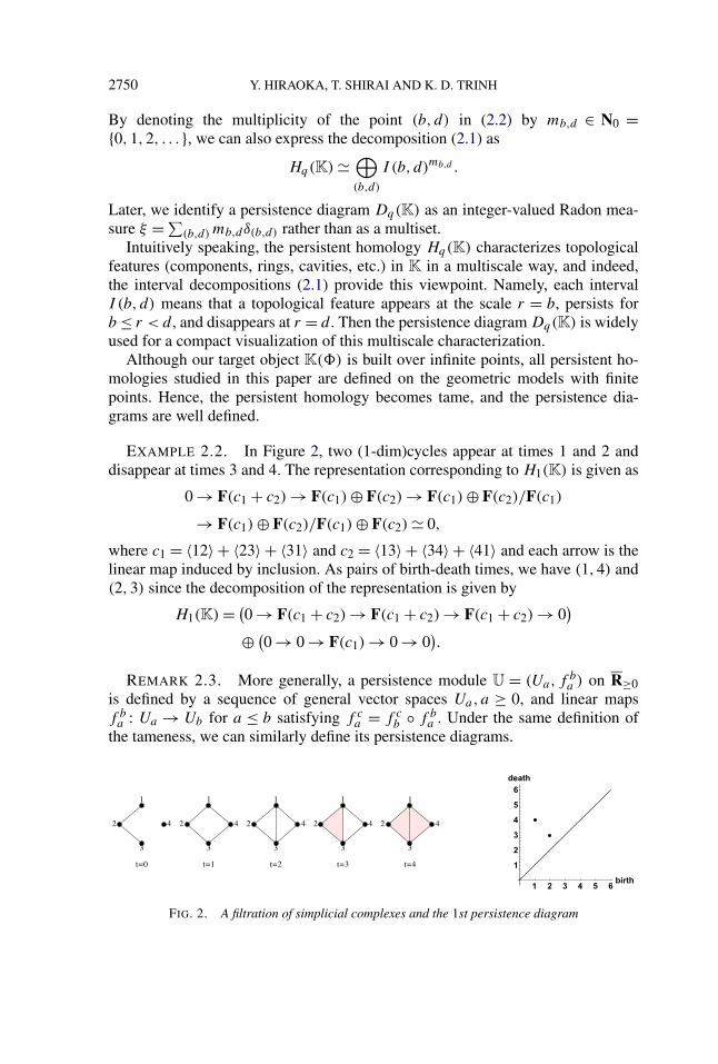
EXAMPLE 2.2. In Figure 2, two (1-dim)cycles appear at times 1 and 2 anddisappear at times 3 and 4. The representation corresponding to H1(K) is given as

0 → F(c1 + c2) → F(c1) ⊕ F(c2) → F(c1) ⊕ F(c2)/F(c1)

→ F(c1) ⊕ F(c2)/F(c1) ⊕ F(c2) � 0,

where c1 = 〈12〉 + 〈23〉 + 〈31〉 and c2 = 〈13〉 + 〈34〉 + 〈41〉 and each arrow is thelinear map induced by inclusion. As pairs of birth-death times, we have (1,4) and(2,3) since the decomposition of the representation is given by

H1(K) = (0 → F(c1 + c2) → F(c1 + c2) → F(c1 + c2) → 0

)⊕ (

0 → 0 → F(c1) → 0 → 0).

REMARK 2.3. More generally, a persistence module U = (Ua, fba ) on R≥0

is defined by a sequence of general vector spaces Ua,a ≥ 0, and linear mapsf b

a : Ua → Ub for a ≤ b satisfying f ca = f c

b ◦ f ba . Under the same definition of

the tameness, we can similarly define its persistence diagrams.

FIG. 2. A filtration of simplicial complexes and the 1st persistence diagram


REMARK 2.4. There is another definition of persistent homology as gradedmodules over a monoid ring for the continuous parameter (resp., a polynomialring for the discrete parameter); see, for example, [18].

REMARK 2.5. The persistent homology Hq(K) defined over the whole � isnot tame in general while Hq(KL) defined over a restriction ��L

is tame. Theo-rem 1.5 informally says that

1

LNHq(KL)

�→ Hq(K) =∫ ⊕

I (x, y)νq(dx dy),

where KL = {K(��L, t)}t≥0, and

∫⊕ denotes the direct integral of interval repre-

sentations (cf. [33]).

REMARK 2.6. In our paper, we use the persistence diagram for represent-ing topological information obtained from filtrations. People sometimes use theso-called barcode representation in which each persistence interval I (b, d) is rep-resented as a barcode [b, d] (cf. [38]). We consider the marginal measure of per-sistence diagram on death times (also on birth times), that is, the induced mea-sure ξ (death) obtained from a measure ξ on by the projection � (x, y) �→y ∈ (0,∞]. The marginal measure ξ

(death)q,L of a persistence diagram ξq,L induces

a (scaled) right-continuous step function fq,L(t) = L−Nξ(death)q,L ([0, t]), which cor-

responds to the one obtained by simulation in [38]. The function fq,L(t) is alsoexpected to converge to a limit fq,∞(t) as L → ∞, however, it does not necessar-

ily coincide with fq(t) := ν(death)q ([0, t]) because of the mass escaping to ∂.

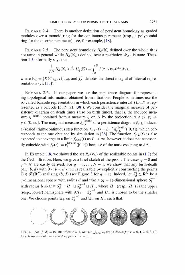
In Example 1.8, we showed the set Rq(κC) of the realizable points in (1.7) forthe Cech filtration. Here, we give a brief sketch of the proof. The cases q = 0 andq ≥ N are easily derived. For q = 1, . . . ,N − 1, we show that any birth-deathpair (b, d) with 0 < b < d < ∞ is realizable by explicitly constructing the points ∈ F (RN) realizing (b, d) (see Figure 3 for q = 1). Indeed, let S

qd ⊂ RN be a

q-dimensional sphere with radius d and take a (q − 1)-dimensional sphere Sq−1b

with radius b so that Sqd = H+ � S

q−1b � H−, where H+ (resp., H−) is the upper

(resp., lower) hemisphere with ∂H± = Sq−1b and H+ is chosen to be the smaller

one. We choose points + on Sq−1b and − on H− such that:

FIG. 3. For (b, d) = (5,10) when q = 1, the set⋃

x∈ Br (x) is drawn for r = 0,1,2,5,8,10.A cycle appears at r = 5 and disappears at r = 10.


(i)⋃

x∈− Br (x) covers H− earlier than r = b;

(ii)⋃

x∈+ Bb(x) covers Sq−1b and is contractive;

(iii)⋃

x∈ Br(x) provides the generator of q-dimensional homology homeo-morphic to S

qd , where = + � −.

Then the birth-death pair of the generator⋃

x∈ Br(x) is exactly (b, d).

2.3. Persistent Betti numbers. For a filtration K, the (r, s)-persistent Bettinumber [10] is defined by

βr,sq (K) = dim

Zq(Kr)

Zq(Kr) ∩ Bq(Ks)(r ≤ s),(2.3)

where Zq(Kr) and Bq(Kr) are the qth cycle group and boundary group, respec-tively. We remark that this is equal to the rank of ιsr : Hq(Kr) → Hq(Ks), because

im ιsr �Zq(Kr)

Bq(Kr)

Zq(Kr)∩Bq(Ks)

Bq(Kr)

� Zq(Kr)

Zq(Kr) ∩ Bq(Ks).

Thus, from the decomposition of the persistent homology, we have

βr,sq (K) = ∑

b≤r,d>s

mb,d .

This means that the (r, s)-persistent Betti number βr,sq (K) counts the number of

birth-death pairs in the persistence diagram Dq(K) located in the gray region ofFigure 4.

LEMMA 2.7. Let U = (Ua, fba ) be a persistence module on R≥0 and let V =

(Va, gba) be its truncation on the interval [r, s], meaning that

Va =

⎧⎪⎪⎨⎪⎪⎩Ur, a ≤ r,

Ua, r ≤ a ≤ s,

Us, a ≥ s,

gba =

⎧⎪⎪⎪⎪⎨⎪⎪⎪⎪⎩f b

a , r ≤ a ≤ b ≤ s,

f sa , r ≤ a ≤ s ≤ b,

f br , a ≤ r ≤ b ≤ s,

f sr , a ≤ r ≤ s ≤ b.

(2.4)

FIG. 4. βr,sq (K) counts the number of generators in the gray region.


For interval decompositions U � ⊕I (b, d)mb,d and V� ⊕I (b, d)nb,d , let

βr,s(U) = ∑b≤r,d>s

mb,d, β0,∞(V) = n0,∞.

Then βr,s(U) = β0,∞(V).

PROOF. This is because βr,s(U) = rankf sr = β0,∞(V). �

Here, we recall the following basic facts in linear algebra for later use.

LEMMA 2.8. Let A, B , U , V be subspaces of a vector space satisfying A ⊂ U

and B ⊂ V . Then

dimU ∩ V

A ∩ B≤ dim

U

A+ dim

V

B.

PROOF. It follows from the formulas dim(U ∩ V ) + dim(U + V ) = dimU +dimV and dim(U/A) = dimU − dimA. �

LEMMA 2.9. Let D = [AB] be a matrix composed by submatrices A and B .Let � be the number of columns in B . Then

rankD ≤ rankA + �, dim kerD ≤ dim kerA + �.

PROOF. Let B = [b1 · · ·b�], where bi is the ith column vector of B , and setD(i) = [Ab1 · · ·bi]. Then, for each i, we have

rankD(i) ≤ rankD(i−1) + 1, dim kerD(i) ≤ dim kerD(i−1) + 1.

Hence, in total, we have the desired inequalities. �

Now, we show a basic estimate on the persistent Betti number for nested filtra-tions K ⊂ K. First, we note the following property.

LEMMA 2.10. Let K be a filtration. For a fixed a > 0, let K = {Kt : t ≥ 0} bea filtration given by

Kt ={Kt, t < a,

Kt ∪ σ, t ≥ a,

where σ is a new simplex added on Ka . Then βr,sq (K) = βr,s

q (K) for dimσ �=q, q + 1. For dimσ = q, q + 1,

∣∣βr,sq (K) − βr,s

q (K)∣∣≤ {

0, Kr = Kr and Ks = Ks,

1 otherwise.


PROOF. We first note that

βr,sq (K) − βr,s

q (K) = dimZq(Kr) − dimZq(Kr) ∩ Bq(Ks)

− (dimZq(Kr) − dimZq(Kr) ∩ Bq(Ks)

)= dim

Zq(Kr)

Zq(Kr)− dim

Zq(Kr) ∩ Bq(Ks)

Zq(Kr) ∩ Bq(Ks).

Hence, the statement is trivial for dimσ �= q, q + 1. Furthermore, when Kr = Kr

and Ks = Ks , we also have βr,sq (K) = βr,s

q (K).Let dimσ = q . Then it follows from Lemma 2.9 that

dimZq(Kr)

Zq(Kr)= dimZq(Kr) − dimZq(Kr) = 0 or 1,

dimBq(Ks)

Bq(Ks)= 0.

Also, from Lemma 2.8, we have

0 ≤ dimZq(Kr) ∩ Bq(Ks)

Zq(Kr) ∩ Bq(Ks)≤ dim

Zq(Kr)

Zq(Kr)+ dim

Bq(Ks)

Bq(Ks)≤ dim

Zq(Kr)

Zq(Kr).

Therefore, |βr,sq (K) − βr,s

q (K)| ≤ 1. The statement for dimσ = q + 1 is similarlyproved. �

LEMMA 2.11. Let K = {Kt }t≥0 and K = {Kt }t≥0 be filtrations with Kt ⊂ Kt

for t ≥ 0. Then∣∣βr,sq (K) − βr,s

q (K)∣∣≤ ∑

j=q,q+1

(|Ks,j \ Ks,j | +∣∣{σ ∈ Ks,j \ Kr,j : tσ ≤ r}∣∣),

where Kt,j (or Kt,j ) is the set of j -simplices in Kt (or Kt ), and tσ (or tσ ) is thebirth time of σ in the filtration K (or K).

PROOF. We first decompose Ks \ Kr = Y � Y c by

Y = (Ks \ Ks) � {σ ∈ Ks \ Kr : tσ ≤ r}, Y c = {σ ∈ Ks \ Kr : r < tσ ≤ tσ }.We use the same notation Yj for the set of j -simplices in Y . For the simplices inKs \ Kr = {σi}Li=1, we assign their indices so that the birth times are in increas-ing order tσ1 ≤ · · · ≤ tσL

and Kr ∪ {σ1, . . . , σ�} becomes a simplicial complex foreach �. We note that tσ ≤ tσ . Furthermore, it suffices to consider the truncations ofK and K on [r, s] from Lemma 2.7.


Now, we inductively construct a sequence of filtrations K = K0 ⊂ K

1 ⊂ · · · ⊂K

L = K. The filtration Ki = {Ki

t : t ≥ 0} is given by adding a simplex σi to Ki−1

at tσi, that is,

Kit =

{Ki−1

t , t < tσi,

Ki−1t ∪ {σi}, t ≥ tσi

.

Then it follows from Lemma 2.10 that |βr,sq (Ki ) − βr,s

q (Ki−1)| ≤ 1 for σi ∈ Y ,since Ki

r �= Ki−1r or Ki

s �= Ki−1s holds. On the other hand, Lemma 2.10 implies

βr,sq (Ki) = βr,s

q (Ki−1) for σ ∈ Y c. Therefore,

∣∣βr,sq (K) − βr,s

q (K)∣∣≤ L∑

i=1

∣∣βr,sq

(K

i)− βr,sq

(K

i−1)∣∣≤ |Yq | + |Yq+1|,

which completes the proof of Lemma 2.11. �

REMARK 2.12. Let �,� ∈ F (RN) with � ⊂ �, and tσ and tσ be the birthtimes of the simplex σ in the κ-filtrations K(�) and K(�), respectively. Thenit is obvious that tσ = tσ if σ ⊂ � ⊂ �. Hence, for the estimate |βr,s

q (K(�)) −βr,s

q (K(�))|, the second term obtained in Lemma 2.11 does not appear under thissetting.

3. General theory of random measures. In this section, we give a brief ac-count of random measures (cf. [24]) and prove Proposition 3.4 which provides asufficient condition for the law of large numbers for random measures to hold. Thenotion of convergence-determining class for vague convergence plays an importantrole in Proposition 3.4. We discuss it separately in Appendix A.

Let S be a locally compact Hausdorff space with countable basis and S be theBorel σ -algebra on S. It is well known that S is a Polish space, that is, a completeseparable metrizable space. If needed, we take a metric ρ which makes S completeand separable. We denote by B(S) the ring of all relatively compact sets in S .A measure μ on (S,S) is said to be a Radon measure if μ(B) < ∞ for everyB ∈ B(S). Let M(S) be the set of all Radon measures on (S,S) and M(S) bethe σ -algebra generated by the mappings M(S) � μ �→ μ(B) ∈ [0,∞) for everyB ∈ B(S).

We say that a sequence {μn}n≥1 ⊂ M(S) converges to μ ∈ M(S) vaguely (orin the vague topology) if 〈μn,f 〉 → 〈μ,f 〉 for every continuous function f withcompact support, where 〈μ,f 〉 = ∫

S f (x) dμ(x). In this case, we write μnv→ μ.

The space M(S) equipped with the vague topology again becomes a Polish spaceand its Borel σ -algebra coincides with M(S).

We denote by N(S) the subset in M(S) of all integer-valued Radon measureson S. Each element in N(S) can be expressed as a sum of delta measures, that is,


μ = ∑i δxi

∈ N(S). We note that the set N(S) is a closed subset of M(S) in thevague topology.

An M(S)-valued [resp., N(S)-valued] random variable ξ = ξω on a probabil-ity space (�,F,P) is called a random measure (resp., point process) on S. Ifλ1(A) := E[ξ(A)] < ∞ for all A ∈ B(S), then λ1 defines a Radon measure andis referred to as the mean measure, or the intensity measure of ξ . Sometimes wedenote it by E[ξ ].

In this paper, two kinds of point processes will appear. One is point processes

on RN as spatial point data and the other is point processes on = {(x, y) ∈ R2 :

0 ≤ x < y ≤ ∞} as persistence diagrams. The former will be denoted by the uppercase letters like � and the latter by the lower case letters like ξ .

The point process � on RN is called stationary, if the distribution P�−1 isinvariant under translations, that is, P�−1

x = P�−1 for any x ∈ RN , where �x isthe translated point process defined by �x(B) = �(B − x) for B ∈ B(RN). ForA ⊂ M(RN), let Ax = {μx : μ ∈ A} be a set of translated measures defined byμx(B) = μ(B − x). Given a point process �, let I be the translation invariantσ -field in N(RN), that is, the class of subsets I ⊂ N(RN) satisfying

P�−1((I \ Ix) ∪ (Ix \ I ))= 0

for all x ∈ RN . Then � is called ergodic if I is trivial, that is, for every I ∈ I ,P�−1(I ) ∈ {0,1}.

From now on and until the end of this section, we fix a space S and write Band M for B(S) and M(S), respectively. For a subset A ⊂ S, we denote by ∂A

and A◦ the boundary and interior of A, respectively. For a measure μ ∈ M, letBμ := {B ∈ B : μ(∂B) = 0} be the class of relatively compact continuity sets ofμ.

LEMMA 3.1 ([24], 15.7.2). Let μ,μ1,μ2, . . . ∈ M. Then the following state-ments are equivalent:

(i) μnv→ μ;

(ii) μn(B) → μ(B) for all B ∈ Bμ;(iii) lim supn→∞ μn(F ) ≤ μ(F) and lim infn→∞ μn(G) ≥ μ(G) for all closed

F ∈ B and open G ∈ B.

LEMMA 3.2 ([24], 15.7.5). A subset C in M is relatively compact in the vaguetopology iff

supμ∈C

μ(B) < ∞ for every B ∈ B.

A class A ⊂ B is called a convergence-determining class (for vague conver-gence) if for every μ ∈ M and every sequence {μn} ⊂M, the condition

μn(A) → μ(A) for all A ∈ A ∩ Bμ


implies the vague convergence μnv→ μ. A class Aμ ⊂ Bμ is called a convergence-

determining class for μ if for any sequence {μn} ⊂M, the condition

μn(A) → μ(A) as n → ∞ for all A ∈ Aμ,

implies that μnv→ μ. By definition, a class A is a convergence-determining class

if and only if for any μ ∈ M, Aμ = A ∩ Bμ is a convergence-determining classfor μ.

We say that a class C has the finite covering property if any subset B ∈ B canbe covered by a finite union of C -sets.

LEMMA 3.3. Let A be a convergence-determining class with finite coveringproperty. Let {μn} be a sequence of measures in M. If μn(A) converges to a finitelimit for any A ∈ A , then there exists a measure μ to which the sequence {μn}converges vaguely.

PROOF. For any relatively compact set B ∈ B, we can find a finite cover{Ai}mi=1 ⊂ A of B so that

lim supn→∞

μn(B) ≤ lim supn→∞

μn

(m⋃

i=1

Ai

)≤ lim

n→∞m∑

i=1

μn(Ai) < ∞.

Therefore, the sequence {μn}n≥1 is relatively compact by Lemma 3.2, and hence,there is a subsequence {μnk

} and μ ∈ M such that μnk

v→ μ, that is, μnk(A) →

μ(A) for every A ∈ Bμ. This together with the assumption implies that μn(A) →μ(A) for every A ∈ A ∩ Bμ. Consequently, μn converges to μ vaguely from thedefinition of convergence-determining class. The proof is complete. �

PROPOSITION 3.4. Let A be a convergence-determining class with finite cov-ering property and the property that for every μ ∈ M, it contains a countableconvergence-determining class for μ. Let {ξn} be a sequence of random measureson S, that is, a sequence of M-valued random variables. Assume that:

(i) E[ξn] ∈ M for all n, and that(ii) for every A ∈ A , there exists cA ∈ [0,∞) such that E[ξn(A)] → cA as

n → ∞.

Then there exists a unique measure μ ∈ M such that the mean measure E[ξn]converges vaguely to μ and μ(A) = cA for A ∈ A ∩ Bμ.

Assume further that for every A ∈ A ,

ξn(A) → cA almost surely as n → ∞.

Then {ξn} converges vaguely to μ almost surely.


PROOF. By Lemma 3.3, there exists a unique measure μ such that E[ξn] con-verges vaguely to μ as n → ∞, and hence μ(A) = cA for A ∈ A ∩ Bμ.

Now let Aμ ⊂ A be a countable convergence-determining class for μ. Thenalmost surely

ξn(A) → μ(A) as n → ∞, for all A ∈ Aμ,

which implies that the sequence {ξn} converges vaguely to μ almost surely. Theproof is complete. �

4. Convergence of persistence diagrams.

4.1. Proof of Theorem 1.11. Let � be a stationary point process on RN havingall finite moments. Let Fq(�A, r) be the number of q-simplices in K(�A, r) andFq(�, r;A) be the number of q-simplices in K(�, r) with at least one vertex inA ⊂ RN . Recall that every q-simplex in K(�, r) containing x must lie in theclosed ball Bρ(r)(x). Therefore, similar to [39], Lemma 3.1, there exists a constantCq,r such that

E[Fq(�A, r)

]≤ E[Fq(�, r;A)

]≤ Cq,r |A|for all bounded Borel sets A, where |A| is the Lebesgue measure of A.

We divide �mM into mN rectangles that are congruent to �M and write asfollows:

�mM =mN⊔i=1

(�M + ci),

where ci is the center of the ith rectangle. We compare K(��mM) with a smaller

filtration K◦(��mM

) :=⊔mN

i=1 K(��M+ci).

Let ψ(L) = E[βr,sq (K(��L

))] for r ≤ s. By Lemma 2.11, we have

(4.1)∣∣βr,s

q

(K(��mM

))− βr,s

q

(K

◦(��mM))∣∣≤ q+1∑

j=q

mN∑i=1

Fj (�(∂�M)(ρ(s))+ci, s).

Here, for A ⊂ RN , we write A(t) = {x ∈ RN : infy∈A ‖x − y‖ ≤ t}. SinceE[Fj (�(∂�M)(ρ(s))+ci

, s)] = O(|(∂�M)(ρ(s)) + ci |) = O(MN−1) as M → ∞, wehave

(4.2)ψ(mM)

(mM)N= ψ(M)

MN+ O

(M−1).

Moreover, for L > L′,

∣∣βr,sq

(K(��L

))− βr,s

q

(K(��L′ )

)∣∣≤ q+1∑j=q

Fj (��L, s;�L \ �L′)


and

E[Fj (��L

, s;�L \ �L′)]= O

(|�L \ �L′ |)= O((

L − L′)LN−1).Then, for fixed M > 0, taking m ∈N such that mM ≤ L < (m + 1)M , we see that

(4.3)ψ(L)

LN= ψ(mM)

(mM)N+ O

(ML−1).

It follows from (4.2) and (4.3) that {L−Nψ(L)}L≥1 is a Cauchy sequence by takingsufficient large M first and then L, which completes the first part of the proof.

Let us assume now that � is ergodic. Since the arguments are similar to thosein the proof of Theorem 3.5 in [39], we only sketch main ideas. By the multidi-mensional ergodic theorem, we see that almost surely as m → ∞,

1

mNβr,s

q

(K

◦(��mM))= 1

mN

mN∑i=1

βr,sq

(K(��M+ci

))→ E

[βr,s

q

(K(��M

))]

,

and for j = q, q + 1,

1

mN

mN∑i=1

Fj (�(∂�M)(ρ(s))+ci, s) → E

[Fj (�(∂�M)(ρ(s)) , s)

]= O(MN−1).

Remark here that the above equations hold for all except a countable set of M (cf.[32], Theorem 1). Therefore, it follows from (4.1) that

lim supm→∞

±1

(mM)Nβr,s

q

(K(��mM

))≤ ±1

MNE[βr,s

q

(K(��M

))]+ O

(M−1).

The rest of the proof is similar to the last step in the first part by noting thatthe following laws of large numbers for Fj (��L

, s), j = q, q + 1, hold (cf. [39],Lemma 3.2),

Fj (��L, s)

Lj→ Fj (s) almost surely as L → ∞.

This completes the second part of the proof. �

COROLLARY 4.1. Let � be a stationary point process on RN having allfinite moments, and ξq,L be the point process on corresponding to the qthpersistence diagram for K(��L

). Then, for every rectangle of the form R =(r1, r2] × (s1, s2], [0, r1] × (s1, s2] ⊂ , there exists a constant CR ∈ [0,∞) suchthat

1

LNE[ξq,L(R)

]→ CR as L → ∞.


1

LNξq,L(R) → CR almost surely as L → ∞.


PROOF. It is a direct consequence of Theorem 1.11 because for R = (r1, r2]×(s1, s2],

ξq,L(R) = βr2,s1q

(K(��L

))− βr2,s2

q

(K(��L

))

+ βr1,s2q

(K(��L

))− βr1,s1

q

(K(��L

)),

and for R = [0, r1] × (s1, s2],ξq,L(R) = βr1,s1

q

(K(��L

))− βr1,s2

q

(K(��L

)). �

4.2. Proof of Theorem 1.5. Let S = = {(x, y) ∈ R2 : 0 ≤ x < y ≤ ∞}. Set

A = {(r1, r2] × (s1, s2], [0, r1] × (s1, s2] ⊂ : 0 ≤ r1 < r2 ≤ s1 < s2 ≤ ∞}

.

We will show in Corollary A.3 that A is a convergence-determining class whichsatisfies the condition in Proposition 3.4. Theorem 1.5 then follows from Proposi-tion 3.4 and Corollary 4.1. �

DEFINITION 4.2. We call the limiting Radon measure νq ∈ M() in The-orem 1.5 the qth persistence diagram for a stationary ergodic point process �

on RN .

EXAMPLE 4.3. Let � be a randomly shifted ZN -lattice with intensity 1,that is, � = ZN + U , where U is a uniform random variable on the unit cube[0,1]N . Then � is a stationary ergodic point process in RN . We compute thelimiting persistence diagram νq of the Cech filtration C(�) = {C(�, r)}r≥0 forq = 1,2, . . . ,N − 1.

For this purpose, we introduce a filtration C(L) = {C(L, r)}r≥0 of cubical com-plexes by

C(L, r) =

⎧⎪⎪⎨⎪⎪⎩CL(L, q),

√q

2≤ r <

√q + 1

2,

CL(L,N), r ≥√

N

2,

where CL(L,N) is the cubical complex consisting of all the elementary cubesin [0,L] × · · · × [0,L] ⊂ RN , and CL(L, q) is the q-dimensional skeleton ofCL(L,N). Here, a cube Q = I1 × · · · × IN ⊂ RN consisting of Ik = [a, a] orIk = [a, a + 1] for some a ∈ Z is called an elementary cube [21]. From the station-arity of � and the homotopy equivalence between C(L, r) and C(ZN ∩[0,L]N, r),it suffices to compute the persistence diagram by using the filtration C(L). We alsonote that (

√q/2,

√q + 1/2) is the only birth-death pair for the qth persistence di-

agram. Therefore, all we need to verify is the multiplicity of that pair with respectto L.


The Euler–Poincaré formula for X = CL(L, q) is given by

q∑k=0

(−1)k|Xk| =q∑

k=0

(−1)kβk(X).(4.4)

The number |Xk| of k-cells in X is given by (see, e.g., [17])

|Xk| =N∑

p=k

(p

k

)Sp(L),

where Sp(x1, . . . , xN) is the elementary symmetric polynomial of degree p andSp(L) is an abbreviation for Sp(L, . . . ,L). On the other hand, since X is homotopyequivalent to a wedge sum of q-spheres, we have β0 = 1 and βk = 0 for k =1, . . . , q − 1. Then it follows from (4.4) that

βq(X) =q∑

k=0

(−1)k+qN∑

p=k

(p

k

)Sp(L) + (−1)q+1,

and hence

βq(X)

LN=

q∑k=0

(−1)k+q

(N

k

)+ O

(L−1)=

(N − 1

q

)+ O

(L−1).

Therefore, the limiting persistence diagram is given by

νq =(N − 1

q

)δ(

√q/2,

√q+1/2).

4.3. The support of νq . In this section, we give some sufficient conditionsboth on κ and � to ensure the positivity of the limiting measure νq . We use thefollowing stability result on persistence diagrams of κ-filtrations (cf. [6, 8]). Here,the qth persistence diagram of the κ-filtration on ∈ F (RN) is simply denotedby Dq().

LEMMA 4.4. Assume that κ is Lipschitz continuous with respect to the Haus-dorff distance, that is, there exists a constant cκ such that∣∣κ(σ ) − κ

(σ ′)∣∣≤ cκdH

(σ,σ ′)

for σ,σ ′ ∈ F (RN). Then, for ,′ ∈ F (RN),

dB

(Dq(),Dq

(′))≤ cκdH

(,′).

Here, dB and dH denote the bottleneck distance and the Hausdorff distance, re-spectively.


See Appendix C for the detail, where we recall definitions of dB and dH andgive a proof of a generalization of this lemma.

Next, we introduce the notion of marker which is a finite point configuration forfinding a specified point in .

DEFINITION 4.5. Let � be a bounded Borel set in RN and (b, d) ∈ . We saythat ∈ F (RN) is a (b, d)-marker in � for the qth persistent homology (PHq ) if(i) ⊂ � and (ii) for any � ∈ F (RN)

(4.5) ξq(��c � )({

(b, d)})≥ ξq(��c)

({(b, d)

})+ 1.

Here, �c denotes the complement of � in RN . For a subset A ⊂ , we also say

that is an A-marker in � if there exists (b, d) ∈ A such that is a (b, d)-markerin �.

EXAMPLE 4.6. (i) Assume that a point (b, d) ∈ is realizable by ∈F (RN). Then there exists M0 > 0 such that is a (b, d)-marker in �M for anyM ≥ M0 because is enough isolated from �c

M for sufficiently large M .(ii) We note that (1/2,

√2/2) ∈ is realized in PH1 by{

(0,0), (1,0), (0,1), (1,1)} ∈ F

(R2)

in the Cech or Rips filtration. It is easy to see that for each c ∈ �1, M =∑x∈Z2∩�M

δx+c is a (1/2,√

2/2)-marker in �M for any sufficiently large M , forexample, M = 3.

THEOREM 4.7. Let

Aq,ε,(b,d) :=∞⋃

M=1

{��M

is a Bε

((b, d)

)-marker in �M for PHq

}and

Sq,ε := {(b, d) ∈ : P(Aq,ε,(b,d)) > 0

}, Sq := ⋂

ε>0

Sq,ε.

Then, Sq ⊂ suppνq .

Before proving Theorem 4.7, we give a lower bound for νq .

LEMMA 4.8. For a closed set A ⊂ ,

(4.6) νq(A) ≥ 1

MNP(��M

is an A-marker in �M for PHq).


PROOF. Let � be a bounded Borel set in RN and (b, d) ∈ . If one could finddisjoint subsets �(1), . . . ,�(k) ⊂ � such that ��(i) is a (b, d)-marker in �(i) foreach i, then

(4.7) ξq(��)({b, d})≥ k.

Indeed, by using (4.5) successively, we have

ξq(��)({

(b, d)})≥ ξq(��\⋃k

j=1 �(j))({

(b, d)})+ k ≥ k.

For L > M > 0 and m = �L/M�, we claim that

(4.8) ξq(��L)(A) ≥

mN∑i=1

1{��M+ciis an A-marker in �M + ci for PHq },

where ci ∈ �L, i = 1,2, . . . ,mN are chosen so that �L ⊃ ⊔mN

i=1(�M + ci).If the right-hand side of (4.8) is equal to k, we have disjoint subsets Ij ⊂{c1, c2, . . . , cmN }, j = 1,2, . . . , J with

∑Jj=1 |Ij | = k such that for every j =

1,2, . . . , J , ��M+c is a (bj , dj )-marker in �M + c for PHq for any c ∈ Ij . Here,(bj , dj ) ∈ A,j = 1,2, . . . , J are all distinct. From (4.7), we have

ξq(��L)(A) ≥

J∑j=1

ξq(��L)({

(bj , dj )})≥

J∑j=1

|Ij | = k,

which implies (4.8).For a closed set A ⊂ , from (4.8), we obtain

νq(A) ≥ lim supL→∞

1

LNE[ξq(��L

)](A)

≥ lim supL→∞

1

LN

mN∑i=1

P(��M+ciis an A-marker in �M + ci for PHq)

= 1

MNP(��M

is an A-marker in �M for PHq).

This completes the proof. �

PROOF OF THEOREM 4.7. If (b, d) ∈ Sq , then for every ε > 0, there existsM = Mε ∈ N such that

P(��M

is a Bε

((b, d)


)> 0.

From (4.6), we see that νq(Bε((b, d))) > 0 for any ε > 0, which implies (b, d) ∈suppνq . Therefore, Sq ⊂ suppνq . �


For a bounded set � ⊂ RN , the restriction N(�) of N(RN) on � can be iden-tified with

⋃∞k=0 �k/ ∼, where ∼ is the equivalence relation induced by permuta-

tions on coordinates. Let � be the probability distribution of homogeneous Pois-son point process with unit intensity. It is clear that the local densities, which aresometimes called Janossy densities, of the restriction of � on � are given by

�|�(dx1 . . . dxn) ={e−|�| dx1 dx2 · · ·dxk on �k,

e−|�| on �0 = {∅}.In other words, for a bounded measurable (local) function f : N(�) → R,

E�[f ] =∞∑

n=0

1

n!∫�n

f (x1, . . . , xn)�|�(dx1 · · ·dxn).

For a probability measure � on N(RN), if �|� is absolutely continuous withrespect to �|� for a bounded set �, then �|� is absolutely continuous with respectto the Lebesgue measure on each �k for every k; thus the Radon–Nikodym densityd�|�/d�|� is defined a.e. on �k for every k.

PROOF OF THEOREM 1.9. Assume that (b, d) ∈ Rq and it is realizable by{y1, . . . , ym}. From continuity of persistence diagram in Lemma 4.4, for anyε > 0 there exists δ > 0 such that ξq({z1, . . . , zm})(Bε({(b, d)})) ≥ 1 for any(z1, . . . , zm) ∈ Bδ(y1) × · · · × Bδ(ym) and the balls {Bδ(yi)}mi=1 are disjoint. FromExample 4.6(i), there exists M ∈ N such that any {z1, . . . , zm} is a Bε((b, d))-marker in �M . Hence, we see that

P(��M

is a Bε

((b, d)


)≥ �|�M

(m⋂

i=1

{�(Bδ(yi) = 1

)}∩{�

(�M

∖ m⋃i=1

Bδ(yi)

)= 0

})

= e−|�M |∫Bδ(y1)×···×Bδ(ym)

f�M(z1, . . . , zm) dz1 · · · dzm

> 0,

where f�M= d�|�M

/d�|�M. Hence, Rq ⊂ Sq ⊂ suppνq by Theorem 4.7. Since

suppνq ⊂ Rq as mentioned after Example 1.8, we conclude that suppνq = Rq .�

Point processes are often specified by the local conditional distributions givena configuration outside, that is, there exists a measurable function q� : N(�) ×N(�c), called a specification, for each bounded Borel set � ∈ B(RN) such thatfor every bounded measurable function f on N(RN)

E�[f |F�c ](ξ) =∞∑

k=0

1

k!∫�k

f (x ∪ ξ�c)q�(x, ξ�c) dx �-a.e.ξ ,


where F�c is the σ -field generated by the mappings ξ �→ �ξ(A),A ∈ B(�c) andx ∪ ξ�c denotes δx1 + · · · + δxk

+ ξ�c if x = (x1, x2, . . . , xk). In this case, the localdensity of � is given by

(4.9)d�|�d�|� (x) = e|�| ·E�

[q�(x, ξ�c)

]for x ∈

∞⋃k=0

�k.

EXAMPLE 4.9. (1) The DLR equations due to Dobrushin–Lanford–Ruelleprovide local conditional distributions of a Gibbs point process. In this formal-ism, a measurable function U� : N(�) × N(�c) → (−∞,∞] is understood asthe conditional energy of particles given a configuration outside of �, if it satisfies

q�(x, ξ�c) = Z�(ξ)−1e−U�(x,ξ�c ),

where

Z�(ξ) =∞∑

k=0

1

k!∫�k

e−U�(x,ξ�c ) dx.

If there exists B ≥ 0 such that −Bk ≤ U(x, ξ�c) < ∞ for any k ≥ 1, x ∈ �k and�-a.e. ξ , then it is easy to see that the local density satisfies the positivity conditionin Theorem 1.9. If U is of hard-core type, that is, U(x, ξ�c) = ∞ for all x in someopen set almost surely, then the positivity condition fails.

(2) For the Ginibre point process and the zeros of the Gaussian entire functiongiven in Example 1.10, Ghosh-Peres [13] showed that both processes exhibit theso-called “rigidity” meaning that for a bounded Borel set � there exists a nonneg-ative integer N(ξ�c) ∈ {0,1,2, . . . } which is measurable with respect to F�c suchthat q(·, ξ�c) is supported on �N(ξ�c ). Roughly speaking, the number of pointsinside � is determined from a given configuration outside of �. Ghosh [12], more-over, showed that there exist positive constants m(ξ�c) and M(ξ�c) such that al-most surely

m(ξ�c)∣∣(x)

∣∣2 ≤ q�(x, ξ�c) ≤ M(ξ�c)∣∣(x)

∣∣2 for a.e. x ∈ �N(ξ�c ),

where (x) =∏1≤i<j≤k(xj − xi) is the Vandermonde determinant. From this in-

equality and (4.9), we have, for any k ≥ 0,d�|�d�|� (x) ≥ e|�|

E�

[m(ξ�c);N(ξ�c) = k

] · ∣∣(x)∣∣2 for x ∈ �k.

Since �(ξ(�) = k) > 0 and m(ξ�c) is positive, the left-hand side is positive almosteverywhere on

⋃∞k=0 �k .

We remark that the Ginibre point process is an important example of determi-nantal point processes. Determinantal (resp., permanental) point processes pro-vides an important class of point processes that are negatively (resp., positively)correlated (cf. [20, 36]). In both cases, the local density can be expressed in termsof the so-called correlation kernel so that for a given kernel one can basically checkwhether the positivity condition is satisfied or not.


5. Central limit theorem for persistent Betti numbers. In this section, let� = P be a homogeneous Poisson point process with unit intensity, and we proveTheorem 1.12. The idea is to apply a result in [31] which shows a central limittheorem for a certain class of functionals defined on Poisson point processes.

We here summarize necessary properties for functionals to achieve the centrallimit theorem. First of all, let us consider a sequence {Wn} of Borel subsets in RN

satisfying the following conditions:

(A1) |Wn| = n for all n ∈ N;(A2)

⋃n≥1

⋂m≥n Wm = RN ;

(A3) limn→∞ |(∂Wn)(r)|/n = 0 for all r > 0;

(A4) there exists a constant γ > 0 such that diam(Wn) ≤ γ nγ .

Given such a sequence, let W = W({Wn}) be the collection of all subsets A in RN

of the form A = Wn + x for some Wn in the sequence and some point x ∈ RN .Let H be a real-valued functional defined on F (RN). The functional H is said

to be translation invariant if it satisfies H(X + y) = H(X ) for any X ∈ F (RN)

and y ∈ RN . Let D0 be the add one cost function

D0H(X ) = H(X ∪ {0})− H(X ), X ∈ F

(RN ),

which is the increment in H caused by inserting a point at the origin. The func-tional H is weakly stabilizing on W if there exists a random variable D(∞) suchthat D0H(PAn)

a.s.−→ D(∞) as n → ∞ for any sequence {An ∈ W}n≥1 tending toRN . The Poisson bounded moment condition on W is given by

sup0∈A∈W

E[(

D0H(PA))4]

< ∞.

Then we restate Theorem 3.1 in [31] in the following form.

LEMMA 5.1 ([31], Theorem 3.1). Let H be a real-valued functional definedon F (RN). Assume that H is translation invariant and weakly stabilizing on W ,and satisfies the Poisson bounded moment condition. Then there exists a constantσ 2 ∈ [0,∞) such that n−1 Var[H(PWn)] → σ 2 and

H(PWn) −E[H(PWn)]n1/2

d→ N(0, σ 2) as n → ∞.

By using Lemma 5.1, we prove the following theorem.

THEOREM 5.2. Let � = P be a homogeneous Poisson point process withunit intensity. Assume that the sequence {Wn} satisfies (A1)–(A4). Then for any0 ≤ r ≤ s < ∞,

βr,sq (K(PWn)) −E[βr,s

q (K(PWn))]n1/2

d→ N(0, σ 2

r,s

)as n → ∞.


In particular, Theorem 1.12 is derived from this theorem by taking Wn = �Ln

with Ln = n1/N .For the proof of Theorem 5.2, the essential part is to show the weak stabilization

of the persistent Betti number βr,sq (K(·)) as a functional on F (RN), on which we

focus below.We remark that, for almost surely, the Poisson point process P consists of infi-

nite points in RN which do not have accumulation points. In view of this property,we first show a stabilization of persistent Betti numbers in the following determin-istic setting.

LEMMA 5.3. Let P be a set of points in RN without accumulation points.Then, for each fixed r ≤ s, there exist constants D∞ and R > 0 such that

D0βr,sq

(K(PBa(0))

)= D∞for all a ≥ R.

PROOF. Let P ′ = P ∪ {0}. Let Kr,a = K(PBa(0), r) be the simplicial complexdefined on PBa(0) with parameter r , and similarly let K ′

r,a = K(P ′Ba(0)

, r).

From the definition (2.3), D0βr,sq (K(PBa(0))) can be expressed as

D0βr,sq

(K(PBa(0))

)= dim

Zq(K′r,a)

Zq(K ′r,a) ∩ Bq(K ′

s,a)− dim

Zq(Kr,a)

Zq(Kr,a) ∩ Bq(Ks,a)

= (dimZq

(K ′

r,a

)− dimZq(Kr,a))

− (dimZq

(K ′

r,a

)∩ Bq

(K ′

s,a

)− dimZq(Kr,a) ∩ Bq(Ks,a)).

Hence, it suffices to show the stabilization with respect to a for dimZq(Kr,a) anddim(Zq(Kr,a) ∩ Bq(Ks,a)) separately.

Let us study dimZq(Kr,a). Since the dimension takes nonnegative integer val-ues, we show the bounded and the nondecreasing properties. First of all, note thatKr,a ⊂ K ′

r,a , and hence Zq(Kr,a) ⊂ Zq(K′r,a). Let us express K ′

r,a as a disjointunion K ′

r,a = Kr,a � K0r,a , where K0

r,a is the set of simplices having the point 0,and let K0

r,a,q = {σ ∈ (K ′r,a)q : 0 ∈ σ }.

Let ∂q,a and ∂ ′q,a be the qth boundary maps on Kr,a and K ′

r,a , respectively. Thenwe can obtain the following block matrix form

∂ ′q,a =

[M1,ρ 0M2,ρ ∂q,a

],(5.1)

where the first columns and rows are arranged by the simplices in K0r,a,q and

K0r,a,q−1, and the second columns and rows correspond to the simplices in Kr,a .


Recall that any simplex σ ∈ K(P, r) containing the point 0 is included inBρ(r)(0). Hence, the set K0

r,a,q becomes independent of a for a ≥ ρ(r), whichwe denote by K0

r,∗,q . From this observation and Lemma 2.9 applied to the matrixform (5.1), we have

dimZq

(K ′

r,a

)− dimZq(Kr,a) ≤ ∣∣K0r,a,q

∣∣= ∣∣K0r,∗,q

∣∣,which gives the boundedness.

In order to show the nondecreasing property, let us consider a homomorphismdefined by

f : Zq(K′r,a1

)

Zq(Kr,a1)� [c] �−→ [c] ∈ Zq(K

′r,a2

)

Zq(Kr,a2)

for a1 ≤ a2. This map is well defined because Zq(Kr,a1) ⊂ Zq(Kr,a2) andZq(K

′r,a1

) ⊂ Zq(K′r,a2

) hold. Suppose that f [c] = 0. Then the cycle c ∈ Zq(K′r,a1

)

is in Zq(Kr,a2). It means that the q-simplices consisting of c do not contain thepoint 0, and hence c ∈ Zq(Kr,a1). This shows that the map f is injective. Fromthis observation, we have the inequality

dimZq

(K ′

r,a1

)/Zq(Kr,a1) ≤ dimZq

(K ′

r,a2

)/Zq(Kr,a2),

which leads to the desired nondecreasing property. This completes the proof of thestabilization of dimZq(Kr,a).

Let us study the stabilization of dim(Zq(Kr,a) ∩ Bq(Ks,a)). The strategy is ba-sically the same as above. It follows from Lemma 2.8 that

dimZq(K

′r,a) ∩ Bq(K ′

s,a)

Zq(Kr,a) ∩ Bq(Ks,a)≤ dim

Zq(K′r,a)

Zq(Kr,a)+ dim

Bq(K ′s,a)

Bq(Ks,a).

Then, from the same reasoning used in dimZq(Kr,a), we have the stabilization|K0

s,a,q+1| = |K0s,∗,q+1| for large a. Hence, we have the boundedness

dimZq

(K ′

r,a

)∩ Bq

(K ′

s,a

)− dimZq(Kr,a) ∩ Bq(Ks,a) ≤ ∣∣K0r,∗,q

∣∣+ ∣∣K0s,∗,q+1

∣∣.Similarly, for sufficiently large a1 ≤ a2, we can show the injectivity of the map

f : Zq(K′r,a1

) ∩ Bq(K ′s,a1

)

Zq(Kr,a1) ∩ Bq(Ks,a1)−→ Zq(K

′r,a2

) ∩ Bq(K ′s,a2

)

Zq(Kr,a2) ∩ Bq(Ks,a2), f [c] = [c],

from which the nondecreasing property follows. This completes the proof of thelemma. �

PROPOSITION 5.4. The functional βr,sq (K(·)) is weakly stabilizing.

PROOF. Let R > 0 be chosen as in Lemma 5.3 and let {An ∈ W}n≥1 be asequence tending to RN . Then there exists n0 ∈ N such that BR(0) ⊂ An for alln ≥ n0.


For n ≥ n0, let us set Lr,n = K(PAn, r). Then, since An is bounded, there existsa > R such that

BR(0) ⊂ An ⊂ Ba(0).

Then, as in the same way used for showing the injectivity in the proof ofLemma 5.3, we can show

Zq(K′r,R)

Zq(Kr,R)⊂ Zq(L

′r,n)

Zq(Lr,n)⊂ Zq(K

′r,a)

Zq(Kr,a),

where Kr,a = K(PBa(0), r) as before. Since the dimensions of Zq(K′r,R)/Zq(Kr,R)

and Zq(K′r,a)/Zq(Kr,a) are equal, for all n ≥ n0

dimZq

(K ′

r,R

)− dimZq(Kr,R) = dimZq

(L′

r,n

)− dimZq(Lr,n).

We can also show that dimZq(L′r,n) ∩ Bq(L

′s,n) − dimZq(Lr,n) ∩ Bq(Ls,n) is in-

variant for n ≥ n0 in a similar manner. This completes the proof. �

PROOF OF THEOREM 5.2. For fixed r ≤ s, we regard the persistent Betti num-ber βr,s

q (K(·)) as a functional on F (RN), and check the three conditions stated inLemma 5.1. First, the translation invariance is obvious, because κ is translationinvariant. Next, let us consider the Poisson bounded moment condition on W . Wenote the following estimate:∣∣D0β

r,sq

(K(PA)

)∣∣= ∣∣βr,sq

(K(PA ∪ {0}))− βr,s

q

(K(PA)

)∣∣≤ ∑

j=q,q+1

∣∣Kj

(PA ∪ {0}, s) \ Kj(PA, s)

∣∣≤ ∑

j=q,q+1

Fj (PBρ(s)(0), s).

Here, the second inequality follows from Lemma 2.11. Then the fourth momentis uniformly bounded because of the finiteness of moments of the Poisson pointprocess on Bρ(s)(0). We showed the weak stabilization in Proposition 5.4. Theproof of Theorem 5.2 is now complete. �

6. Conclusions. In this paper, we studied a convergence of persistence dia-grams and persistent Betti numbers for stationary point processes, and a centrallimit theorem of persistent Betti numbers for homogeneous Poisson point process.Several important problems are still yet to be solved:

1. We showed the existence of limiting persistence diagram for simplicialcomplexes built over stationary ergodic point processes. Such convergence resultscan be expected for more general random simplicial/cell complexes studied in [17,18]. It would also be important to investigate the rate of convergence from thestatistical and computational point of view.


2. Attractiveness/repulsiveness of point processes are reflected on persistencediagrams (see Figure 1). For example, the mass of the limiting persistence diagramνq for negatively correlated point process seems to become more concentrated thanthat for positively correlated point process.

3. The moments of the limiting persistence diagram,∫ |y − x|nνq(dx dy),

should be studied. Other properties of limiting persistence diagrams such as conti-nuity, absolute continuity/singularity, comparison, etc. should also be investigatedthoroughly for practical purposes (cf. [16, 26]).

4. The central limit theorem for persistent Betti numbers (even for usual Bettinumbers) is only proved for Poisson point processes. It could be extended to moregeneral stationary point processes. We also expect that a scaled persistence dia-gram converges to a Gaussian field on .

APPENDIX A: CONVERGENCE-DETERMINING CLASS FOR VAGUECONVERGENCE

We provide a sufficient condition for a class of B-sets to be a convergencedetermining class for vague convergence. We use the same notation as in Section 3.Assume that a class A ⊂ B is closed under finite intersections. Let us define

R(A ) ={⋃

finite

Ai : Ai ∈ A

}.

Then R(A ) is closed under both finite intersections and finite unions. Further-more, if μn(A) → μ(A) for all A ∈ A , then so does for all A ∈ R(A ), because

μ

(m⋃

i=1

Ai

)=∑

i

μ(Ai) −∑i �=j

μ(Ai ∩ Aj) + · · · + (−1)m−1μ

(m⋂

i=1

Ai

).

LEMMA A.1. Assume that a class A is closed under finite intersections, andthat:

(i) each open set G ∈ B is a countable union of R(A )-sets, and(ii) each closed set F ∈ B is a countable intersection of R(A )-sets.

If μn(A) → μ(A) for all A ∈ A , then μn converges vaguely to μ. In particular,the class A is a convergence-determining class for μ provided that A ⊂ Bμ.

PROOF. Let G ∈ B be an open set. By assumption, there are sets Ai ∈ R(A )

such that

G =∞⋃i=1

Ai.


Given ε > 0, choose an m such that

μ

(m⋃

i=1

Ai

)> μ(G) − ε.

Then we have

μ(G) − ε < μ

(m⋃

i=1

Ai

)= lim

n→∞μn

(m⋃

i=1

Ai

)≤ lim inf

n→∞ μn(G).

Since ε is arbitrary, we get

μ(G) ≤ lim infn→∞ μn(G).

Now for a closed set F ∈ B, take Ai ∈ R(A ) such that

F =∞⋂i=1

Ai.

Since Ai ∈ B, for given ε > 0, we can choose m large enough such that

μ(F) + ε > μ

(m⋂

i=1

Ai

).

Then it follows from⋂m

i=1 Ai ∈ R(A ) that

μ(F) + ε > μ

(m⋂

i=1

Ai

)= lim

n→∞μn

(m⋂

i=1

Ai

)≥ lim sup

n→∞μn(F ).

Letting ε → 0, we get

μ(F) ≥ lim supn→∞

μn(F ).

Therefore, the conclusion follows from Lemma 3.1. �

For given A , let Ax,ε be the class of A -sets satisfying x ∈ A◦ ⊂ A ⊂ Bε(x),where A◦ is the interior of A. Let ∂Ax,ε be the class of their boundaries, that is,∂Ax,ε = {∂A : A ∈ Ax,ε}.

The following theorem gives a sufficient condition for a class A to be aconvergence-determining class for vague convergence of Radon measures (seeTheorem 2.4 in [1] for an analogous result on weak convergence of probabilitymeasures).

THEOREM A.2. Suppose that A is closed under finite intersections and, foreach x ∈ S and ε > 0, ∂Ax,ε contains either ∅ or uncountably many disjoint sets.Then A is a convergence-determining class. Moreover, for any measure μ ∈ M,A contains a countable convergence-determining class for μ.


PROOF. Fix an arbitrary μ ∈ M, and let Aμ = A ∩ Bμ be the class of μ-continuity sets in A . Since

∂(A ∩ B) ⊂ (∂A) ∪ (∂B),

Aμ is again closed under finite intersections.Let G ∈ B be an open set. For x ∈ G, choose ε > 0 such that Bε(x) ⊂ G. By the

assumption, if ∂Ax,ε does not contain ∅, then it must contain uncountably manydisjoint sets. Hence, in either case, ∂Ax,ε contains a set ∂Ax of μ-measure 0, orAx ∈ Aμ. Therefore, G can be written as

G = ⋃x∈G

A◦x = ⋃

x∈G

Ax.

Since S is a separable metric space, there is a countable subcollection {A◦xi

} of{A◦

x : x ∈ G} which covers G, namely,

G =∞⋃i=1

A◦xi

.

Let {Gi}∞i=1 be a countable basis of S. For each i, we have just shown that thereare countable sets {Ai,j }∞j=1 ⊂ Aμ such that

Gi =∞⋃

j=1

A◦i,j =

∞⋃j=1

Ai,j .

Set

A ′μ =

{⋂finite

Ai,j

}.

Then A ′μ ⊂ Aμ is countable and closed under finite intersections. The remaining

task is to show that A ′μ satisfies the two conditions in Lemma A.1. The condition

for open sets is clear from the construction of A ′μ.

Next, let F ∈ B be a closed (thus compact) set. For each ε > 0, let

F (ε) ={x ∈ S : d(x,F ) = inf

y∈Fρ(x, y) ≤ ε

}.

Then F = ⋂∞p=1 F

( 1p). We claim that, for each ε > 0, there exist m = m(ε) and a

collection of sets {Ck}mk=1 ⊂ A ′μ such that

F ⊂m⋃

k=1

Ck ⊂ F (ε).

Indeed, for each x ∈ F , there is a pair (ix, jx) such that x ∈ A◦ix ,jx

⊂ Aix,jx ⊂Gix ⊂ Bε(x). Let Cx = Aix,jx . Then

F ⊂ ⋃x∈F

C◦x .


Since F is compact, there is a finite collection {C◦xk

}mk=1 such that

F ⊂m⋃

k=1

C◦xk

.

Finally, note that C◦xk

⊂ Cxk⊂ F (ε), we have

F ⊂m⋃

k=1

Cxk⊂ F (ε).

Therefore, the condition for closed sets in Lemma A.1 is satisfied, which completesthe proof of Theorem A.2. �

COROLLARY A.3. The class

A = {(r1, r2] × (s1, s2], [0, r2] × (s1, s2] ⊂ : 0 ≤ r1 ≤ r2 ≤ s1 ≤ s2 ≤ ∞}

satisfies the conditions of Proposition 3.4, namely, for any measure μ, it containsa countable convergence determining class for μ.

PROOF. It suffices to check the conditions in Theorem A.2. It is clear that Ais closed under finite intersection and ∂Ax,ε contains uncountably many disjointsets for any x ∈ and ε > 0. �

APPENDIX B: SIMPLICIAL COMPLEX AND HOMOLOGY

B.1. Simplicial complex. We first introduce a combinatorial object calledsimplicial complex. Let P = {1, . . . , n} be a finite set (not necessary to be pointsin a metric space). A simplicial complex with the vertex set P is defined by acollection K of nonempty subsets in P satisfying the following properties:

(i) {i} ∈ K for i = 1, . . . , n, and(ii) if σ ∈ K and ∅ �= τ ⊂ σ , then τ ∈ K .

Each subset σ with q + 1 vertices is called a q-simplex. We denote the set of q-simplices by Kq . A subcollection T ⊂ K which also becomes a simplicial complexis called a subcomplex of K .

EXAMPLE B.1. Figure 5 shows two polyhedra of simplicial complexes:

K = {{1}, {2}, {3}, {1,2}, {1,3}, {2,3}, {1,2,3}},T = {{1}, {2}, {3}, {1,2}, {1,3}, {2,3}}.


FIG. 5. The polyhedra of the simplicial complexes K (left) and T (right).

B.2. Homology. The procedure to define homology is summarized as fol-lows:

1. Given a simplicial complex K , build a chain complex C∗(K). This is analgebraization of K characterizing the boundary.

2. Define homology by quotienting out certain subspaces in C∗(K) charac-terized by the boundary.

We begin with the procedure 1 by assigning orientations on simplices. When wedeal with a q-simplex σ = {i0, . . . , iq} as an ordered set, there are (q + 1)! order-ings on σ . For q > 0, we define an equivalence relation ij0, . . . , ijq ∼ i�0, . . . , i�q

on two orderings of σ such that they are mapped to each other by even permu-tations. By definition, two equivalence classes exist, and each of them is calledan oriented simplex. An oriented simplex is denoted by 〈ij0, . . . , ijq 〉, and itsopposite orientation is expressed by adding the minus −〈ij0, . . . , ijq 〉. We write〈σ 〉 = 〈ij0, . . . , ijq 〉 for the equivalence class including ij0 < · · · < ijq . For q = 0,we suppose that we have only one orientation for each vertex.

Let F be a field. We construct a F-vector space Cq(K) as

Cq(K) = SpanF{〈σ 〉 | σ ∈ Kq

}for Kq �= ∅ and Cq(K) = 0 for Kq = ∅. Here, SpanF(A) for a set A is avector space over F such that the elements of A formally form a basis of thevector space. Furthermore, we define a linear map called the boundary map∂q : Cq(K) → Cq−1(K) by the linear extension of

∂q〈i0, . . . , iq〉 =q∑

�=0

(−1)�〈i0, . . . , i�, . . . , iq〉,(B.1)

where i� means the removal of the vertex i�. We can regard the linear map ∂q

as algebraically capturing the (q − 1)-dimensional boundary of a q-dimensionalobject.

For example, the image of the 2-simplex 〈σ 〉 = 〈1,2,3〉 is given by ∂2〈σ 〉 =〈2,3〉 − 〈1,3〉 + 〈1,2〉, which is the boundary of σ (see Figure 5).

In practice, by arranging some orderings of the oriented q- and (q − 1)-simplices, we can represent the boundary map as a matrix

Mq = (Mσ,τ )σ∈Kq−1,τ∈Kq


with the entry Mσ,τ = 0,±1 given by the coefficient in (B.1). For the simplicialcomplex K in Example B.1, the matrix representations M1 and M2 of the boundarymaps are given by

M2 =⎡⎣ 1

1−1

⎤⎦ , M1 =⎡⎣−1 0 −1

1 −1 00 1 1

⎤⎦ .(B.2)

Here, the 1-simplices (resp. 0-simplices) are ordered by 〈1,2〉, 〈2,3〉, 〈1,3〉 (resp.,〈1〉, 〈2〉, 〈3〉).

We call a sequence of the vector spaces and linear maps

· · · �� Cq+1(K)∂q+1

�� Cq(K)∂q

�� Cq−1(K) �� · · ·the chain complex C∗(K) of K . As an easy exercise, we can show ∂q ◦ ∂q+1 = 0for every q . Hence, the subspaces Zq(K) = ker∂q and Bq(K) = im∂q+1 satisfyBq(K) ⊂ Zq(K). Then the qth (simplicial) homology is defined by taking the quo-tient space

Hq(K) = Zq(K)/Bq(K).

Intuitively, the dimension of Hq(K) counts the number of q-dimensional holes inK and each generator of the vector space Hq(K) corresponds to these holes. Weremark that the homology as a vector space is independent of the orientations ofsimplices.

For a subcomplex T of K , the inclusion map ι : T ↪→ K naturally induces alinear map in homology ιq : Hq(T ) → Hq(K). Namely, an element [c] ∈ Hq(T )

is mapped to [c] ∈ Hq(K), where the equivalence class [c] is taken in each vectorspace.

For example, the simplicial complex K in Example B.1 has

Z1(K) = SpanF[1 1 −1 ]T = B1(K)

from (B.2). Hence, H1(K) = 0, meaning that there are no 1-dimensional hole(ring) in K . On the other hand, since Z1(T ) = Z1(K) and B1(T ) = 0, we haveH1(T ) � F, meaning that T consists of one ring. Hence, the induced linear mapι1 : H1(T ) → H1(K) means that the ring in T disappears in K under T ↪→ K .

APPENDIX C: CONTINUITY OF PERSISTENCE DIAGRAMS OFκ-COMPLEXES

We give a stability result for persistence diagrams of κ-filtrations which extendsthe stability result obtained in [6]. The notation used here follows the paper [6].We first recall the definition of the Hausdorff distance and the bottleneck distance.The Hausdorff distance dH on F (RN) for σ,σ ′ ∈ F (RN) is given by

dH

(σ,σ ′)= max

{maxx∈σ

infx′∈σ ′

∥∥x − x′∥∥, maxx′∈σ ′ inf

x∈σ

∥∥x − x′∥∥}.


We define the �∞-metric on by d∞((b1, d1), (b2, d2)) = max(|b1 − b2|, |d1 −d2|), where ∞ − ∞ = 0. For (b, d) ∈ , we define d∞((b, d), ∂) = (d − b)/2.For finite multisets X and Y in , a partial matching between X and Y is a sub-set M ⊂ X × Y such that for every x ∈ X there is at most one y ∈ Y such that(x, y) ∈ M and for every y ∈ Y there is at most one x ∈ X such that (x, y) ∈ M .An x ∈ X (resp., y ∈ Y ) is unmatched if there is no y ∈ Y (resp., x ∈ X) such that(x, y) ∈ M . We say that a partial matching M is δ-matching if d∞(x, y) ≤ δ forevery (x, y) ∈ M , d∞(x, ∂) ≤ δ if x ∈ X is unmatched, and d∞(y, ∂) ≤ δ ify ∈ Y is unmatched.

The bottleneck distance is defined as follows:

dB(X,Y ) := inf{δ > 0 : there exists a δ-matching between X and Y }.For ,′ ∈ F (RN) and κ, κ ′ : F (RN) → [0,∞], we define two complexes

Kκ() = {Kκ(, t)

}t≥0, Kκ ′

(′)= {

Kκ ′(′, t

)}t≥0.

Let C be a correspondence between and ′, that is, C ⊂ × ′ such thatp1(C) = and p2(C) = ′, where pi is the projection onto the ith coordinate fori = 1,2. We define the transpose CT of C, which is also a correspondence, by

CT := {(x′, x

) ∈ ′ × : (x, x′) ∈ C}.

A correspondence C defines a map from F () to F (′) as

C(σ) = {x′ ∈ ′ : (x, x′) ∈ C,x ∈ σ

}.

The distortion of C is defined as

dis(C) := max{

supσ⊂

∣∣κ(σ ) − κ ′(C(σ))∣∣, sup

σ ′⊂′

∣∣κ(CT (σ ′))− κ ′(σ ′)∣∣}.LEMMA C.1. If dis(C) ≤ ε, then Hq(Kκ()) and Hq(Kκ ′(′)) are ε-

interleaving.

PROOF. Assume that σ ∈ Kκ(, t) and κ(σ ) ≤ t . Then it follows from|κ(σ ) − κ ′(C(σ))| ≤ ε that

κ ′(σ ′)≤ κ ′(C(σ))≤ κ(σ ) + ε ≤ t + ε for any σ ′ ⊂ C(σ),

which implies σ ′ ∈ Kκ ′(′, t + ε), and hence C is ε-simplicial from Kκ() toKκ ′(′). Symmetrically, CT is also ε-simplicial. Therefore, the conclusion followsfrom Proposition 4.2 in [6]. �

Let us define

(C.1) S((κ,),

(κ ′,′)) := sup

σ⊂,σ ′⊂′dH (σ,σ ′)≤dH (,′)

∣∣κ(σ ) − κ ′(σ ′)∣∣.We remark that S((κ,), (κ ′,′)) = ‖κ − κ ′‖∞ if = ′.


LEMMA C.2. Let C denote the correspondence defined by C = {(x, x′) ∈ ×′ : ‖x − x′‖ ≤ dH (,′)}. Then

dis(C) ≤ S((κ,),

(κ ′,′)).

PROOF. We easily see that

supσ⊂

dH

(σ,C(σ)

)≤ dH

(,′) and sup

σ ′⊂′dH

(CT (σ ′), σ ′)≤ dH

(,′),

which implies the assertion. �

For Dq(κ,) = Dq(Kκ()) and Dq(κ ′,′) = Dq(Kκ ′(′)), we obtain the fol-lowing continuity result.

THEOREM C.3.

(C.2) dB

(Dq(κ,),Dq

(κ ′,′))≤ S

((κ,),

(κ ′,′)).

PROOF. It follows from Lemma C.2 and Lemma C.1 that Hq(Kκ()) andHq(Kκ ′(′)) are S((κ,), (κ ′,′))-interleaving. Therefore, we obtain (C.2) from[5]. �

COROLLARY C.4. Suppose that κ is Lipschitz continuous with respect to dH ,that is, there exists a constant γ > 0 such that∣∣κ(σ ) − κ

(σ ′)∣∣≤ γ dH

(σ,σ ′) for σ,σ ′ ∈ F

(RN

).

Then

(C.3) dB

(Dq(κ,),Dq

(κ,′))≤ γ dH

(,′).

PROOF. From the assumption and (C.1), we see that

S((κ,),

(κ,′))≤ γ dH

(,′).

Therefore, (C.3) follows. �

Acknowledgment. The authors would like to thank Shu Kanazawa, IppeiObayashi and Kenkichi Tsunoda for useful discussions. The authors would alsolike to thank the associate editor and the referee for many valuable commentswhich really help to improve this paper.


REFERENCES

[1] BILLINGSLEY, P. (1999). Convergence of Probability Measures, 2nd ed. Wiley Series in Prob-ability and Statistics: Probability and Statistics. Wiley, New York. MR1700749

[2] BŁASZCZYSZYN, B. and YOGESHWARAN, D. (2015). Clustering comparison of point pro-cesses, with applications to random geometric models. In Stochastic Geometry, Spa-tial Statistics and Random Fields. Lecture Notes in Math. 2120 31–71. Springer, Cham.MR3330572

[3] BOBROWSKI, O. and KAHLE, M. (2014). Topology of random simplicial complexes: A survey.Topology in Statistical Inference, the Proceedings of Symposia in Applied Mathematics.To appear. Available at arXiv:1409.4734.

[4] CARLSSON, G. (2009). Topology and data. Bull. Amer. Math. Soc. (N.S.) 46 255–308.MR2476414

[5] CHAZAL, F., DE SILVA, V., GLISSE, M. and OUDOT, S. (2016). The Structure and Stabilityof Persistence Modules. SpringerBriefs in Mathematics. Springer, Cham. MR3524869

[6] CHAZAL, F., DE SILVA, V. and OUDOT, S. (2014). Persistence stability for geometric com-plexes. Geom. Dedicata 173 193–214. MR3275299

[7] CHIU, S. N., STOYAN, D., KENDALL, W. S. and MECKE, J. (2013). Stochastic Geometryand Its Applications, 3rd ed. Wiley Series in Probability and Statistics. Wiley, Chichester.MR3236788

[8] COHEN-STEINER, D., EDELSBRUNNER, H. and HARER, J. (2007). Stability of persistencediagrams. Discrete Comput. Geom. 37 103–120. MR2279866

[9] EDELSBRUNNER, H. and HARER, J. L. (2010). Computational Topology. Amer. Math. Soc.,Providence, RI. MR2572029

[10] EDELSBRUNNER, H., LETSCHER, D. and ZOMORODIAN, A. (2002). Topological persistenceand simplification. Discrete Comput. Geom. 28 511–533. MR1949898

[11] GAMEIRO, M., HIRAOKA, Y., IZUMI, S., KRAMAR, M., MISCHAIKOW, K. and NANDA, V.(2015). A topological measurement of protein compressibility. Jpn. J. Ind. Appl. Math.32 1–17. MR3318898

[12] GHOSH, S. (2012). Rigidity and Tolerance in Gaussian zeroes and Ginibre eigenvalues: Quan-titative estimates. Preprint. Available at arXiv:1211.3506.

[13] GHOSH, S. and PERES, Y. (2017). Rigidity and tolerance in point processes: Gaussian zerosand Ginibre eigenvalues. Duke Math. J. 166 1789–1858. MR3679882

[14] GRESCHONIG, G. and SCHMIDT, K. (2000). Ergodic decomposition of quasi-invariant proba-bility measures. Colloq. Math. 84/85 495–514. MR1784210

[15] HATCHER, A. (2002). Algebraic Topology. Cambridge Univ. Press, Cambridge. MR1867354[16] HIRAOKA, Y., NAKAMURA, T., HIRATA, A., ESCOLAR, E. G., MATSUE, K. and NISHIURA,

Y. (2016). Hierarchical structures of amorphous solids characterized by persistent homol-ogy. Proc. Natl. Acad. Sci. USA 113 7035–7040.

[17] HIRAOKA, Y. and SHIRAI, T. (2016). Tutte polynomials and random-cluster models inBernoulli cell complexes. In Stochastic Analysis on Large Scale Interacting Sys-tems. RIMS Kôkyûroku Bessatsu, B59 289–304. Res. Inst. Math. Sci. (RIMS), Kyoto.MR3675939

[18] HIRAOKA, Y. and SHIRAI, T. (2017). Minimum spanning acycle and lifetime of persistenthomology in the Linial–Meshulam process. Random Structures Algorithms 51 315–340.MR3683365

[19] HIRAOKA, Y. and TSUNODA, K. (2016). Limit theorems for random cubical homology.Preprint. Available at arXiv:1612.08485.

[20] HOUGH, J. B., KRISHNAPUR, M., PERES, Y. and VIRÁG, B. (2009). Zeros of Gaussian An-alytic Functions and Determinantal Point Processes. University Lecture Series 51. Amer.Math. Soc., Providence, RI. MR2552864

http://www.ams.org/mathscinet-getitem?mr=1700749


http://arxiv.org/abs/arXiv:1409.4734


















[21] KACZYNSKI, T., MISCHAIKOW, K. and MROZEK, M. (2004). Computational Homology. Ap-plied Mathematical Sciences 157. Springer, New York. MR2028588

[22] KAHLE, M. (2011). Random geometric complexes. Discrete Comput. Geom. 45 553–573.MR2770552

[23] KAHLE, M. (2014). Topology of random simplicial complexes: A survey. In Algebraic Topol-ogy: Applications and New Directions. Contemp. Math. 620 201–221. Amer. Math. Soc.,Providence, RI. MR3290093

[24] KALLENBERG, O. (1986). Random Measures, 4th ed. Akademie-Verlag, Berlin. MR0854102[25] KARAMCHANDANI, N., MANJUNATH, D., YOGESHWARAN, D. and IYER, S. K. (2006).

Evolving random geometric graph models for mobile wireless networks. In 2006 4th In-ternational Symposium on Modeling and Optimization in Mobile, Ad Hoc and WirelessNetworks 1–7. IEEE.

[26] KUSANO, G., FUKUMIZU, K. and HIRAOKA, Y. (2016). Persistence weighted Gaussian kernelfor topological data analysis. In Proceedings of the 33rd International Conference onMachine Learning 2004–2013.

[27] MIYOSHI, N. and SHIRAI, T. (2014). A cellular network model with Ginibre configured basestations. Adv. in Appl. Probab. 46 832–845. MR3254344

[28] NAKAMURA, T., HIRAOKA, Y., HIRATA, A., ESCOLAR, E. G. and NISHIURA, Y. (2015). Per-sistent homology and many-body atomic structure for medium-range order in the glass.Nanotechnol. 26 304001.

[29] OWADA, T. and ADLER, R. J. (2017). Limit theorems for point processes under geomet-ric constraints (and topological crackle). Ann. Probab. 45 2004–2055. DOI:10.1214/16-AOP1106. MR3650420

[30] PENROSE, M. (2003). Random Geometric Graphs. Oxford Studies in Probability 5. OxfordUniv. Press, Oxford. MR1986198

[31] PENROSE, M. D. and YUKICH, J. E. (2001). Central limit theorems for some graphs in com-putational geometry. Ann. Appl. Probab. 11 1005–1041. MR1878288

[32] PUGH, C. and SHUB, M. (1971). Ergodic elements of ergodic actions. Compos. Math. 23 115–122. MR0283174

[33] REED, M. and SIMON, B. (1978). Methods of Modern Mathematical Physics. IV. Analysis ofOperators. Academic Press, New York. MR0493421

[34] RILEY, S., EAMES, K., ISHAM, V., MOLLISON, D. and TRAPMAN, P. (2015). Five challengesfor spatial epidemic models. Epidemics 10 68–71.

[35] SAADATFAR, M., TAKEUCHI, H., ROBINS, V., FRANCOIS, N. and HIRAOKA, Y. (2017). Poreconfiguration landscape of granular crystallization. Nat. Commun. 8 15082.

[36] SHIRAI, T. and TAKAHASHI, Y. (2003). Random point fields associated with certain Fredholmdeterminants. I. Fermion, Poisson and boson point processes. J. Funct. Anal. 205 414–463. DOI:10.1016/S0022-1236(03)00171-X. MR2018415

[37] TRINH, K. D. (2017). A remark on the convergence of Betti numbers in the thermodynamicregime. Pac. J. Math. Ind. 9 Art. 4, 7. DOI:10.1186/s40736-017-0029-0. MR3620264

[38] YOGESHWARAN, D. and ADLER, R. J. (2015). On the topology of random complexes builtover stationary point processes. Ann. Appl. Probab. 25 3338–3380. MR3404638

[39] YOGESHWARAN, D., SUBAG, E. and ADLER, R. J. (2017). Random geometric complexes inthe thermodynamic regime. Probab. Theory Related Fields 167 107–142. MR3602843

[40] ZOMORODIAN, A. and CARLSSON, G. (2005). Computing persistent homology. DiscreteComput. Geom. 33 249–274. MR2121296






https://doi.org/10.1214/16-AOP1106






https://doi.org/10.1016/S0022-1236(03)00171-X


https://doi.org/10.1186/s40736-017-0029-0





https://doi.org/10.1214/16-AOP1106


Y. HIRAOKA

ADVANCED INSTITUTE FOR MATERIALS RESEARCH

TOHOKU UNIVERSITY

2-1-1, KATAHIRA, AOBA-KU

SENDAI, 980-8577JAPAN

E-MAIL: [email protected]

T. SHIRAI

K. D. TRINH

INSTITUTE OF MATHEMATICS FOR INDUSTRY

KYUSHU UNIVERSITY

744, MOTOOKA, NISHI-KU

FUKUOKA, 819-0395JAPAN

E-MAIL: [email protected]@imi.kyushu-u.ac.jp

mailto:[email protected]



limit theorems for persistence diagrams

Documents