confidence sets for persistence diagrams · confidence sets for persistence diagrams by brittany...

arX

iv:1

303.

7117

v3 [

mat

h.ST

] 2

0 N

ov 2

014

The Annals of Statistics

2014, Vol. 42, No. 6, 2301–2339DOI: 10.1214/14-AOS1252c© Institute of Mathematical Statistics, 2014

CONFIDENCE SETS FOR PERSISTENCE DIAGRAMS

By Brittany Terese Fasy*,1, Fabrizio Lecci†,2,Alessandro Rinaldo†,2, Larry Wasserman†,3,Sivaraman Balakrishnan† and Aarti Singh†

Tulane University* and Carnegie Mellon University†

Persistent homology is a method for probing topological proper-ties of point clouds and functions. The method involves tracking thebirth and death of topological features (2000) as one varies a tuningparameter. Features with short lifetimes are informally considered tobe “topological noise,” and those with a long lifetime are consideredto be “topological signal.” In this paper, we bring some statisticalideas to persistent homology. In particular, we derive confidence setsthat allow us to separate topological signal from topological noise.

1. Introduction. Topological data analysis (TDA) refers to a collectionof methods for finding topological structure in data [Carlsson (2009), Edels-brunner and Harer (2010)]. TDA has been used in protein analysis, imageprocessing, text analysis, astronomy, chemistry and computer vision, as wellas in other fields.

One approach to TDA is persistent homology, a branch of computationaltopology that leads to a plot called a persistence diagram. This diagram canbe thought of as a summary statistic, capturing multi-scale topological fea-tures. This paper studies the statistical properties of persistent homology.Homology detects the connected components, tunnels, voids, etc., of a topo-logical space M. Persistent homology measures these features by assigninga birth and a death value to each feature. For example, suppose we sam-ple Sn = X1, . . . ,Xn from an unknown distribution P . We are interestedin estimating the homology of the support of P . One method for doing sowould be to take the union of the set of balls centered at the points in Sn

as we do in the supplementary material [Fasy et al. (2014)]; however, to do

Received March 2013; revised June 2014.1Supported in part by NSF Grant CCF-1065106.2Supported in part by NSF CAREER Grant DMS-11-49677.3Supported in part by Air Force Grant FA95500910373, NSF Grant DMS-08-06009.AMS 2000 subject classifications. Primary 62G05, 62G20; secondary 62H12.Key words and phrases. Persistent homology, topology, density estimation.

This is an electronic reprint of the original article published by theInstitute of Mathematical Statistics in The Annals of Statistics,2014, Vol. 42, No. 6, 2301–2339. This reprint differs from the original inpagination and typographic detail.

1

http://arxiv.org/abs/1303.7117v3

http://www.imstat.org/aos/

http://dx.doi.org/10.1214/14-AOS1252

http://www.imstat.org

http://www.ams.org/msc/

http://www.imstat.org

http://www.imstat.org/aos/

http://dx.doi.org/10.1214/14-AOS1252

2 B. T. FASY ET AL.

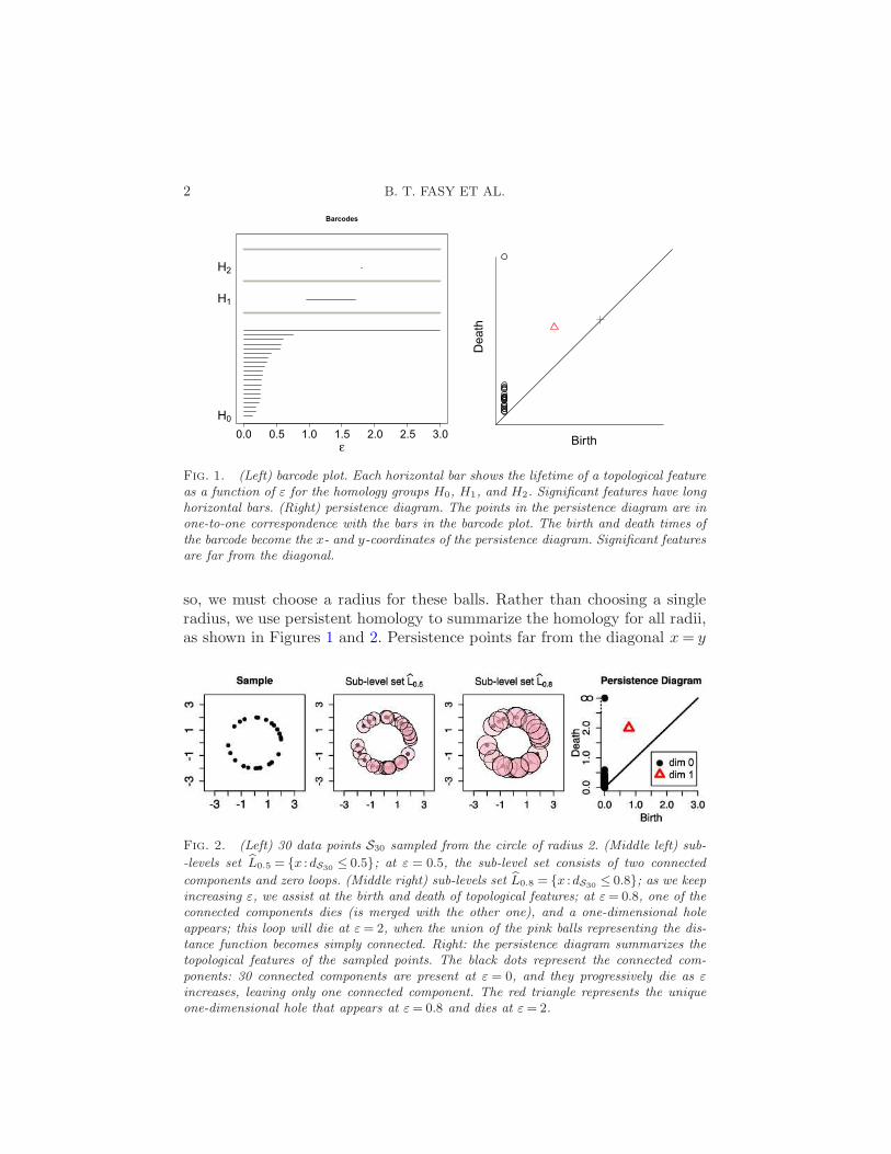
Fig. 1. (Left) barcode plot. Each horizontal bar shows the lifetime of a topological featureas a function of ε for the homology groups H0, H1, and H2. Significant features have longhorizontal bars. (Right) persistence diagram. The points in the persistence diagram are inone-to-one correspondence with the bars in the barcode plot. The birth and death times ofthe barcode become the x- and y-coordinates of the persistence diagram. Significant featuresare far from the diagonal.

so, we must choose a radius for these balls. Rather than choosing a singleradius, we use persistent homology to summarize the homology for all radii,as shown in Figures 1 and 2. Persistence points far from the diagonal x= y

Fig. 2. (Left) 30 data points S30 sampled from the circle of radius 2. (Middle left) sub-

-levels set L0.5 = x :dS30≤ 0.5; at ε = 0.5, the sub-level set consists of two connected

components and zero loops. (Middle right) sub-levels set L0.8 = x :dS30≤ 0.8; as we keep

increasing ε, we assist at the birth and death of topological features; at ε= 0.8, one of theconnected components dies (is merged with the other one), and a one-dimensional holeappears; this loop will die at ε= 2, when the union of the pink balls representing the dis-tance function becomes simply connected. Right: the persistence diagram summarizes thetopological features of the sampled points. The black dots represent the connected com-ponents: 30 connected components are present at ε = 0, and they progressively die as ε

increases, leaving only one connected component. The red triangle represents the uniqueone-dimensional hole that appears at ε= 0.8 and dies at ε= 2.

INFERENCE FOR HOMOLOGY 3

represent topological features common to a long interval of radii. We definepersistent homology precisely in Section 2.

One of the key challenges in persistent homology is to find a way toseparate the noise from the signal in the persistence diagram, and this papersuggests several statistical methods for doing so. In particular, we provide aconfidence set for the persistence diagram P corresponding to the distancefunction to a topological space M using a sample from a distribution Psupported on M. The confidence set has the form C = Q :W∞(P ,Q)≤ cn,where Q varies over the set of all persistence diagrams, P is an estimate

of the persistence diagram constructed from the sample, W∞ is a metricon the space of persistence diagrams, called the bottleneck distance, andcn is an appropriate, data-dependent quantity. In addition, we study theupper level sets of density functions by computing confidence sets for theirpersistence diagrams.

Goals. There are two main goals in this paper. The first is to introducepersistent homology to statisticians. The second is to derive confidence setsfor certain key quantities in persistent homology. In particular, we derive asimple method for separating topological noise from topological signal. Themethod has a simple visualization: we only need to add a band around thediagonal of the persistence diagram. Points in the band are consistent withbeing noise. We focus on simple, synthetic examples in this paper as proofof concept.

Related work. Some key references in computational topology are [Bu-benik and Kim (2007), Carlsson (2009), Ghrist (2008), Carlsson and Zomoro-dian (2009), Edelsbrunner and Harer (2008), Chazal and Oudot (2008),Chazal et al. (2011)]. An Introduction to homology can be found in Hatcher(2002). The probabilistic basis for random persistence diagrams is studiedin Mileyko, Mukherjee and Harer (2011) and Turner et al. (2014). Otherrelevant probabilistic results can be found in Kahle (2009, 2011), Penrose(2003), Kahle and Meckes (2013). Some statistical results for homology andpersistent homology include Bubenik et al. (2010), Blumberg et al. (2012),Balakrishnan et al. (2011), Joshi et al. (2011), Bendich, Mukherjee andWang (2010), Chazal et al. (2010), Bendich, Galkovskyi and Harer (2011),Niyogi, Smale and Weinberger (2008, 2011). The latter paper considers achallenging example which involves a set of the form in Figure 8 (top left),which we consider later in the paper. Heo, Gamble and Kim (2012) containsa detailed analysis of data on a medical procedure for upper jaw expansionthat uses persistent homology as part of a nonlinear dimension reduction ofthe data. Chazal et al. (2013b) is closely related to this paper; they find con-vergence rates for persistence diagrams computed from data sampled from a

4 B. T. FASY ET AL.

distribution on a metric space. As the authors point out, finding confidenceintervals that follow from their methods is a challenging problem becausetheir probability inequalities involve unknown constants. Restricting our at-tention to manifolds embedded in R

D, we are able to provide several methodsto compute confidence sets for persistence diagrams.

Outline. We define persistent homology formally in Section 2 and provideadditional details in the supplementary material [Fasy et al. (2014)]. Thestatistical model is defined in Section 3. Several methods for constructingconfidence intervals are presented in Section 4. Section 5 illustrates the ideaswith a few numerical experiments. Proofs are contained in Section 6. Finally,Section 7 contains concluding remarks.

Notation. We write an bn if there exists c > 0 such that an ≤ cbn forall large n. We write an ≍ bn if an bn and bn an. For any x∈R

D and anyr ≥ 0, B(x, r) denotes the D-dimensional ball of radius r > 0 centered at x.For any closed set A⊂R

D, we define the (Euclidean) distance function

dA(x) = infy∈A

‖y − x‖2.(1)

In addition, for any ε≥ 0, the Minkowski sum is defined as

A⊕ ε=⋃

x∈AB(x, ε) = x :dA(x)≤ ε.(2)

The reach of A—denoted by reach(A)—is the largest ε≥ 0 such that eachpoint in A⊕ ε has a unique projection onto A [Federer (1959)]. If f is a real-valued function, we define the upper level set x :f(x)≥ t, the lower levelset x :f(x)≤ t and the level set x :f(x) = t. If A is measurable, we writeP (A) for the probability of A. For more general events A, P(A) denotes theprobability of A on an appropriate probability space. In particular, if A isan event in the n-fold probability space under random sampling, then P(A)means probability under the product measure P × · · · × P . In some places,we use symbols like c, c1,C, . . . , as generic positive constants. Finally, if twosets A and B are homotopic, we write A∼=B.

2. Brief introduction to persistent homology. In this section, we pro-vide a brief overview of persistent homology. In the supplementary material[Fasy et al. (2014)], we provide a more details on relevant concepts fromcomputational topology; however, for a more complete coverage of persis-tent homology, we refer the reader to Edelsbrunner and Harer (2010).

Given a real-valued function f , persistent homology describes how thetopology of the lower level sets f−1(−∞, t] change as t increases from −∞ to∞. In particular, persistent homology describes f with a multiset of points


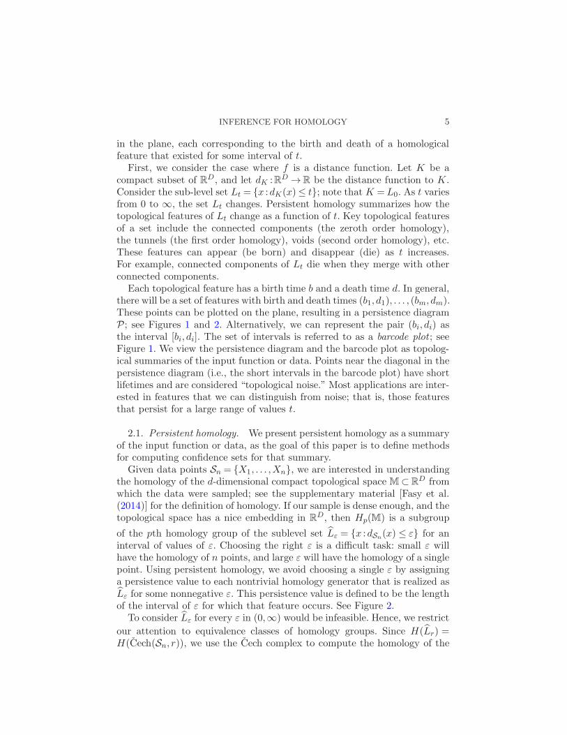
in the plane, each corresponding to the birth and death of a homologicalfeature that existed for some interval of t.

First, we consider the case where f is a distance function. Let K be acompact subset of RD, and let dK :RD →R be the distance function to K.Consider the sub-level set Lt = x :dK(x)≤ t; note that K =L0. As t variesfrom 0 to ∞, the set Lt changes. Persistent homology summarizes how thetopological features of Lt change as a function of t. Key topological featuresof a set include the connected components (the zeroth order homology),the tunnels (the first order homology), voids (second order homology), etc.These features can appear (be born) and disappear (die) as t increases.For example, connected components of Lt die when they merge with otherconnected components.

Each topological feature has a birth time b and a death time d. In general,there will be a set of features with birth and death times (b1, d1), . . . , (bm, dm).These points can be plotted on the plane, resulting in a persistence diagramP ; see Figures 1 and 2. Alternatively, we can represent the pair (bi, di) asthe interval [bi, di]. The set of intervals is referred to as a barcode plot ; seeFigure 1. We view the persistence diagram and the barcode plot as topolog-ical summaries of the input function or data. Points near the diagonal in thepersistence diagram (i.e., the short intervals in the barcode plot) have shortlifetimes and are considered “topological noise.” Most applications are inter-ested in features that we can distinguish from noise; that is, those featuresthat persist for a large range of values t.

2.1. Persistent homology. We present persistent homology as a summaryof the input function or data, as the goal of this paper is to define methodsfor computing confidence sets for that summary.

Given data points Sn = X1, . . . ,Xn, we are interested in understandingthe homology of the d-dimensional compact topological space M⊂R

D fromwhich the data were sampled; see the supplementary material [Fasy et al.(2014)] for the definition of homology. If our sample is dense enough, and thetopological space has a nice embedding in R

D, then Hp(M) is a subgroup

of the pth homology group of the sublevel set Lε = x :dSn(x) ≤ ε for aninterval of values of ε. Choosing the right ε is a difficult task: small ε willhave the homology of n points, and large ε will have the homology of a singlepoint. Using persistent homology, we avoid choosing a single ε by assigninga persistence value to each nontrivial homology generator that is realized asLε for some nonnegative ε. This persistence value is defined to be the lengthof the interval of ε for which that feature occurs. See Figure 2.

To consider Lε for every ε in (0,∞) would be infeasible. Hence, we restrict

our attention to equivalence classes of homology groups. Since H(Lr) =H(Cech(Sn, r)), we use the Cech complex to compute the homology of the

6 B. T. FASY ET AL.

lower level sets; see the supplementary material [Fasy et al. (2014)] for thedefinition of a Cech complex. Let r1, . . . , rk be the set of radii such that thecomplexes Cech(Sn, ri) and Cech(Sn, ri− ε) are not identical for sufficientlysmall ε. Letting K0 =∅, Kk+1 be the maximal simplicial complex defined

on Sn, and Ki = Cech(Sn, (ri + ri−1)/2), the sequence of complexes is theCech filtration of dSn . For all s < t, there is a natural inclusion is,t :Ks →Kt

that induces a group homomorphism i∗s,t :Hp(Ks)→Hp(Kt). Thus we havethe following sequence of homology groups:

Hp(|K0|)→Hp(|K1|)→ · · · →Hp(|Kn|).(3)

We say that a homology class [α] represented by a p-cycle α is born at Ks if[α] is not supported in Kr for any r < s, but is nontrivial in Hp(|Ks|). Theclass [α] born at Ks dies going into Kt if t is the smallest index such thatthe class [α] is supported in the image of i∗s−1,t. The birth at s and death att of [α] is recorded as the point (s, t) in the pth persistence diagram Pp(dSn),which we now formally define.

Definition 1 (Persistence diagram). Given a function f :X → R, de-fined for a triangulable subspace of RD, the pth persistence diagram Pp(f)

is the multiset of points in the extended plane R2, where R=R∪−∞,+∞,

such that the each point (s, t) in the diagram represents a distinct topolog-ical feature that existed in Hp(f

−1((−∞, r])) for r ∈ [s, t). The persistencebarcode is a multiset of intervals that encodes the same information as thepersistence diagram by representing the point (s, t) as the interval [s, t].

In sum, the zero-dimensional diagram P0(f) records the birth and deathof components of the lower level sets; more generally, the p-dimensionaldiagram Pp(f) records the p-dimensional holes of the lower level sets. We letP(f) be the overlay of all persistence diagrams for f ; see Figures 2 and 3, forexamples, of persistent homology of one-dimensional and two-dimensionaldistance functions.

In the supplementary material [Fasy et al. (2014)], we see that the homol-ogy of a lower level set is equivalent to a Cech complex and can be estimatedby a Vietoris–Rips complex. Therefore, in Section 5, we use the Vietoris–Rips filtration to compute the confidence sets for persistence diagrams ofdistance functions.

2.2. Stability. We say that the persistence diagram is stable if a smallchange in the input function produces a small change in the persistencediagram. There are many variants of the stability result for persistencediagrams, as we may define different ways of measuring distance betweenfunctions or distance between persistence diagrams. We are interested in us-ing the L∞-distance between functions and the bottleneck distance between


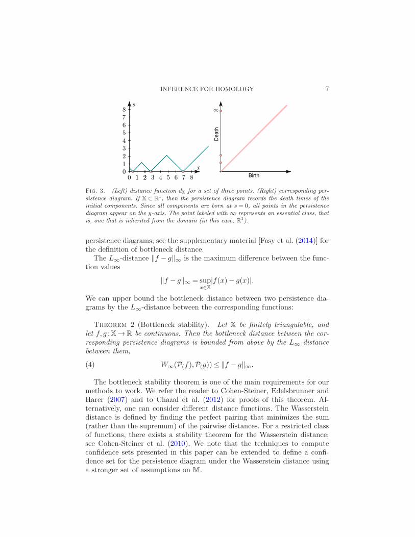
Fig. 3. (Left) distance function dX for a set of three points. (Right) corresponding per-sistence diagram. If X ⊂ R

1, then the persistence diagram records the death times of theinitial components. Since all components are born at s = 0, all points in the persistencediagram appear on the y-axis. The point labeled with ∞ represents an essential class, thatis, one that is inherited from the domain (in this case, R1).

persistence diagrams; see the supplementary material [Fasy et al. (2014)] forthe definition of bottleneck distance.

The L∞-distance ‖f − g‖∞ is the maximum difference between the func-tion values

‖f − g‖∞ = supx∈X

|f(x)− g(x)|.

We can upper bound the bottleneck distance between two persistence dia-grams by the L∞-distance between the corresponding functions:

Theorem 2 (Bottleneck stability). Let X be finitely triangulable, andlet f, g :X→R be continuous. Then the bottleneck distance between the cor-responding persistence diagrams is bounded from above by the L∞-distancebetween them,

W∞(P(f),P(g))≤ ‖f − g‖∞.(4)

The bottleneck stability theorem is one of the main requirements for ourmethods to work. We refer the reader to Cohen-Steiner, Edelsbrunner andHarer (2007) and to Chazal et al. (2012) for proofs of this theorem. Al-ternatively, one can consider different distance functions. The Wassersteindistance is defined by finding the perfect pairing that minimizes the sum(rather than the supremum) of the pairwise distances. For a restricted classof functions, there exists a stability theorem for the Wasserstein distance;see Cohen-Steiner et al. (2010). We note that the techniques to computeconfidence sets presented in this paper can be extended to define a confi-dence set for the persistence diagram under the Wasserstein distance usinga stronger set of assumptions on M.

8 B. T. FASY ET AL.

2.3. Hausdorff distance. Let A,B be compact subsets of RD. One wayto measure the distance between these sets is to take the Hausdorff distance,denoted by H(A,B), which is the maximum Euclidean distance from a pointin one set to the closest point in the other set,

H(A,B) = maxmaxx∈A

miny∈B

‖x− y‖,maxx∈B

miny∈A

‖x− y‖

= infǫ :A⊂B ⊕ ǫ and B ⊂A⊕ ǫ.The stability result Theorem 2 is key. Let M be a d-manifold embedded

in a compact subset X of RD. If S is any subset of M, PS is the persistencediagram based on the lower level sets x :dS(x)≤ t, and P is the persistencediagram based on the lower level sets x :dM(x)≤ t, then, by Theorem 2,

W∞(PS ,P)≤ ‖dS − dM‖∞ =H(S,M).(5)

We bound H(S,M) to obtain a bound on W∞(PS ,P). In particular, weobtain a confidence set for W∞(PS ,P) by deriving a confidence set forH(S,M). Thus the stability theorem reduces the problem of inferring per-sistent homology to the problem of inferring Hausdorff distance. Indeed,much of this paper is devoted to the latter problem. We would like to pointout that the Hausdorff distance plays an important role in many statisticalproblems. Examples include Cuevas (2009), Cuevas, Febrero and Fraiman(2001), Cuevas and Fraiman (1997, 1998), Cuevas, Fraiman and Pateiro-Lopez (2012), Cuevas and Rodrıguez-Casal (2004), Mammen and Tsybakov(1995). Our methods could potentially be useful for these problems as well.

3. Statistical model. As mentioned above, we want to estimate the ho-mology of a set M. We do not observe M directly; rather, we observe asample Sn = X1, . . . ,Xn from a distribution P that is concentrated onor near M ⊂ R

D. For example, suppose M is a circle. Then the homologyof the data set Sn is not equal to the homology of M; however, the setLε = x :dSn(x) ≤ ε =

⋃ni=1B(Xi, ε), where B(x, ε) denotes the Euclidean

ball of radius ε centered at x, captures the homology of M for an interval ofvalues ε. Figure 2 shows Lε for increasing values of ε.

Let X1, . . . ,Xni.i.d.∼ P where Xi ∈ R

D. Let M denote the d-dimensionalsupport of P . Let us define the following quantities:

ρ(x, t) =P (B(x, t/2))

td, ρ(t) = inf

x∈Mρ(x, t).(6)

We assume that ρ(x, t) is a continuous function of t, and we define

ρ(x,↓ 0) = limt→0

ρ(x, t), ρ= limt→0

ρ(t).(7)

Note that if P has continuous density p with respect to the uniformmeasure onM, then ρ∝ infx∈M p(x). Until Section 4.4, we make the followingassumptions:


Assumption A1. M is d-dimensional compact manifold (with no bound-ary), embedded in R

D and reach(M)> 0. (The definition of reach was givenin Section 1.)

Assumption A2. For each x ∈M, ρ(x, t) is a bounded continuous func-tion of t, differentiable for t ∈ (0, t0) and right differentiable at zero. More-over, ∂ρ(x, t)/∂t exists and is bounded away from zero and infinity for t inan open neighborhood of zero. Also, for some t0 > 0 and some C1 and C2,we have

supx

sup0≤t≤t0

∣∣∣∣∂ρ(x, t)

∂t

∣∣∣∣≤C1 <∞ and sup0≤t≤t0

|ρ′(t)| ≤C2 <∞.(8)

Remarks. The reach of M does not appear explicitly in the results asthe dependence is implicit and does not affect the rates in the asymptotics.Note that if P has a density p with respect to the Hausdorff measure on M,then Assumption A2 is satisfied as long as p is smooth and bounded awayfrom zero. Assumption A1 guarantees that as ε→ 0, the covering numberN(ε) satisfies N(ε) ≍ (1/ε)d . However, the conditions are likely strongerthan needed. For example, it suffices that M be compact and d-rectifiable.See, for example, Mattila (1995) and Ambrosio, Fusco and Pallara (2000).

Recall that the distance function is dM(x) = infy∈M ‖x − y‖, and let Pbe the persistence diagram defined by the lower level sets x :dM(x) ≤ ε.Our target of inference is P . Let P denote the persistence diagram of thex :dSn(x)≤ ε where Sn = X1, . . . ,Xn. We regard P as an estimate of P .

Our main goal is to find a confidence interval for W∞(P, P) as this impliesa confidence set for the persistence diagram.

Until Section 4.4, we assume that the dimension of M is known and thatthe support of the distribution is M which is sometimes referred to as thenoiseless case. These assumptions may seem unrealistic to statisticians butare, in fact, common in computational geometry. In Section 4.4, we weakenthe assumptions. Specifically, we allow outliers, which means there may bepoints not on M. Bendich, Galkovskyi and Harer (2011) show that methodsbased on the Cech complex perform poorly when there are outliers. Instead,we estimate the persistent homology of the upper level sets of the densityfunction. We shall see that the methods in Section 4.4 are quite robust.

4. Confidence sets. Given α ∈ (0,1), we will find cn ≡ cn(X1, . . . ,Xn)such that

lim supn→∞

P(W∞(P ,P)> cn)≤ α.(9)

10 B. T. FASY ET AL.

It then follows that Cn = [0, cn] is an asymptotic 1−α confidence set for the

bottleneck distance W∞(P ,P), that is,

lim infn→∞

P(W∞(P ,P) ∈ [0, cn])≥ 1−α.(10)

Recall that, from Theorem 2 and the fact that ‖dM− dSn‖∞ =H(Sn,M),we have

W∞(P ,P)≤H(Sn,M),(11)

where Sn = X1, . . . ,Xn is the sample and H is the Hausdorff distance.Hence it suffices to find cn such that

lim supn→∞

P(H(Sn,M)> cn)≤ α.(12)

The confidence set Cn is a subset of all persistence diagrams whose dis-tance to P is at most cn,

Cn = P :W∞(P , P)≤ cn.

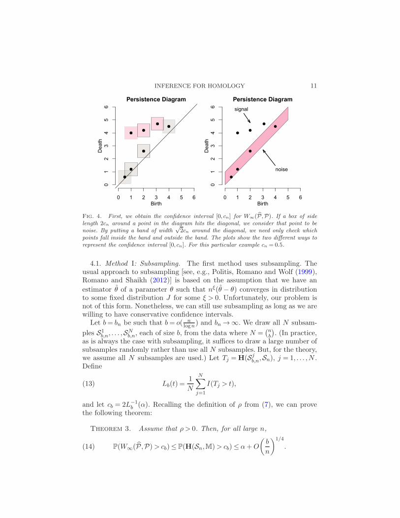
We can visualize Cn by centering a box of side length 2cn at each point p onthe persistence diagram. The point p is considered indistinguishable fromnoise if the corresponding box, formally defined as q ∈ R

2 :d∞(p, q)≤ cn,intersects the diagonal. Alternatively, we can visualize the confidence set byadding a band of width

√2cn around the diagonal of the persistence diagram

P . The interpretation is this: points in the band are not significantly differ-ent from noise. Points above the band can be interpreted as representing asignificant topological feature. That is, if the confidence set for a point onthe diagram hits the diagonal, then we cannot rule out that the lifetime ofthat feature is 0, and we consider it to be noise. (This is like saying thatif a confidence interval for a treatment effect includes 0, then the effect isnot distinguishable form “no effect.”) This leads to the diagrams shown inFigure 4.

Remark. This simple dichotomy of “signal” and “noise” is not the onlyway to quantify the uncertainty in the persistence diagram. Indeed, somepoints near the diagonal may represent interesting structure. One can imag-ine endowing each point in the diagram with a confidence set, possibly ofdifferent sizes and shapes. But for the purposes of this paper, we focus onthe simple method described above.

The first three methods that we present are based on the persistencediagram constructed from the Cech complex. The fourth method takes adifferent approach completely and is based on density estimation. We definethe methods in this section; we illustrate them in Section 5.


Fig. 4. First, we obtain the confidence interval [0, cn] for W∞(P ,P). If a box of sidelength 2cn around a point in the diagram hits the diagonal, we consider that point to benoise. By putting a band of width

√2cn around the diagonal, we need only check which

points fall inside the band and outside the band. The plots show the two different ways torepresent the confidence interval [0, cn]. For this particular example cn = 0.5.

4.1. Method I: Subsampling. The first method uses subsampling. Theusual approach to subsampling [see, e.g., Politis, Romano and Wolf (1999),Romano and Shaikh (2012)] is based on the assumption that we have an

estimator θ of a parameter θ such that nξ(θ − θ) converges in distributionto some fixed distribution J for some ξ > 0. Unfortunately, our problem isnot of this form. Nonetheless, we can still use subsampling as long as we arewilling to have conservative confidence intervals.

Let b= bn be such that b= o( nlogn) and bn →∞. We draw all N subsam-

ples S1b,n, . . . ,SN

b,n, each of size b, from the data where N =(nb

). (In practice,

as is always the case with subsampling, it suffices to draw a large number ofsubsamples randomly rather than use all N subsamples. But, for the theory,we assume all N subsamples are used.) Let Tj =H(Sj

b,n,Sn), j = 1, . . . ,N .Define

Lb(t) =1

N

N∑

j=1

I(Tj > t),(13)

and let cb = 2L−1b (α). Recalling the definition of ρ from (7), we can prove

the following theorem:

Theorem 3. Assume that ρ > 0. Then, for all large n,

P(W∞(P ,P)> cb)≤ P(H(Sn,M)> cb)≤ α+O

(b

n

)1/4

.(14)


4.2. Method II: Concentration of measure. The following lemma is sim-ilar to theorems in Devroye and Wise (1980), Cuevas, Febrero and Fraiman(2001) and Niyogi, Smale and Weinberger (2008).

Lemma 4. For all t > 0,

P(W∞(P ,P)> t)≤ P(H(Sn,M)> t)≤ 2d

ρ(t/2)tdexp(−nρ(t)td),(15)

where ρ(t) is defined in (6). If, in addition, t <minρ/(2C2), t0, then

P(H(Sn,M)> t)≤ 2d+1

tdρexp

(−n

ρtd

2

).(16)

Hence if tn(α)<minρ/(2C2), t0 is the solution to the equation

2d+1

tdnρexp

(−n

ρtdn2

)= α,(17)

then

P(W∞(P ,P)> tn(α))≤ P(H(Sn,M)> tn(α))≤ α.

Remarks. From the previous lemma, it follows that, setting tn =(4ρ

lognn )1/d,

P(H(Sn,M)> tn)≤2d−1

n logn,

for all n large enough. The right-hand side of (15) is known as the Lam-bert function [Lambert (1758)]. Equation (17) does not admit a closed formsolution, but can be solved numerically.

To use the lemma, we need to estimate ρ. Let Pn be the empirical measureinduced by the sample Sn, given by

Pn(A) =1

n

n∑

i=1

IA(Xi),

for any measurable Borel set A ⊂ RD. Let rn be a positive small number

and consider the plug-in estimator of ρ,

ρn =mini

Pn(B(Xi, rn/2))

rdn.(18)

Our next result shows that, under our assumptions and provided that thesequence rn vanishes at an appropriate rate as n→∞, ρn is a consistentestimator of ρ.


Theorem 5. Let rn ≍ (logn/n)1/(d+2). Then

ρn − ρ=OP (rn).

Remark. We have assumed that d is known. It is also possible to esti-mate d, although we do not pursue that extension here.

We now need to use ρn to estimate tn(α) as follows. Assume that n iseven, and split the data randomly into two halves, Sn = S1,n ⊔S2,n. Let ρ1,nbe the plug-in estimator of ρ computed from S1,n, and define t1,n to solvethe equation

2d+1

tdρ1,nexp

(−ntdρ1,n

2

)= α.(19)

Theorem 6. Let P2 be the persistence diagram for the distance functionto S2,n, then

P(W∞(P2,P)> t1,n)≤ P(H(S2,n,M)> t1,n)(20)

≤ α+O

(logn

n

)1/(2+d)

,

where the probability P is with respect to both the joint distribution of theentire sample and the randomness induced by the sample splitting.

In practice, we have found that solving (19) for tn without splitting thedata also works well although we do not have a formal proof. Another wayto define tn which is simpler but more conservative, is to define

tn =

(2

nρnlog

(n

α

))1/d

.(21)

Then tn = un(1 +O(ρn − ρ)) where un = ( ρnρn

log(nα ))1/d, and so

P(H(Sn,M)> tn) = P(H(Sn,M)> un) +O

(logn

n

)1/(2+d)

≤ α+O

(logn

n

)1/(2+d)

.

4.3. Method III: The method of shells. The dependence of the previousmethod on the parameter ρ makes the method very fragile. If the densityis low in even a small region, then the method above is a disaster. Here


we develop a sharper bound based on shells of the form x :γj < ρ(x,↓ 0)<γj+1 where we recall from (6) and (7) that

ρ(x,↓ 0) = limt→0

ρ(x, t) = limt→0

P (B(x, t/2))

td.

Let G(v) = P (ρ(X,↓ 0)≤ v), and let g(v) =G′(v).

Theorem 7. Suppose that g is bounded and has a uniformly bounded,continuous derivative. Then for any t≤ ρ/(2C1),

P(W∞(P ,P)> t)≤ P (H(Sn,M)> t)(22)

≤ 2d+1

td

∫ ∞

ρ

g(v)

ve−nvtd/2 dv.

Let K be a smooth, symmetric kernel satisfying the conditions in Gineand Guillou (2002) (which includes all the commonly used kernels), and let

g(v) =1

n

n∑

i=1

1

bK

(v− Vi

b

),(23)

where b > 0, Vi = ρ(Xi, rn), and

ρ(x, rn) =Pn(B(x, rn/2))

rdn.

Theorem 8. Let rn = ( lognn )1/(d+2).

(1) We have that

supv|g(v)− g(v)|=OP

(b2 +

√logn

nb+

rnb2

).

Hence if we choose b≡ bn ≍ r1/4n , then

supv|g(v)− g(v)|=OP

(logn

n

)1/(2(d+2))

.

(2) Suppose that n is even and that ρ > 0. Assume that g is strictlypositive over its support [ρ,B]. Randomly split the data into two halves:Sn = (S1,n,S2,n). Let g1,n and ρ1,n be estimators of g and ρ, respectively,computed from the first half of the data, and define t1,n to be the solution ofthe equation

2d+1

td1,n

∫ ∞

ρn

g(v)

ve−nvtd/2 dv = α.(24)


Then

P(W∞(P2,P)> t1,n)≤ P(H(S2,n,M)> t1,n)≤ α+O(rn),(25)

where P2 is the persistence diagram associated to S2,n and the probabilityP is with respect to both the joint distribution of the entire sample and therandomness induced by the sample splitting.

4.4. Method IV: Density estimation. In this section, we take a com-pletely different approach. We use the data to construct a smooth densityestimator, and then we find the persistence diagram defined by a filtrationof the upper level sets of the density estimator; see Figure 5. A differentapproach to smoothing based on diffusion distances is discussed in Bendich,Galkovskyi and Harer (2011).

Again, let X1, . . . ,Xn be a sample from P . Define

ph(x) =

∫

M

1

hDK

(‖x− u‖2h

)dP (u).(26)

Then ph is the density of the probability measure Ph which is the convolution

Ph = P ⋆Kh where Kh(A) = h−DK(h−1A) and K(A) =

∫AK(t)dt. That is,

Ph is a smoothed version of P . Our target of inference in this section is Ph,the persistence diagram of the upper level sets of ph. The standard estimatorfor ph is the kernel density estimator

ph(x) =1

n

n∑

i=1

1

hDK

(‖x−Xi‖2h

).(27)

It is easy to see that E(ph(x)) = ph(x). Let us now explain why Ph is ofinterest.

Fig. 5. We plot the persistence diagram corresponding to the upper level set filtrationof the function f(x). For consistency, we swap the birth and death axes so all persistencepoints appear above the line y = x. The point born first does not die, but for convenience wemark it’s death at f(x) = 0. This is analogous to the point marked with ∞ in our previousdiagrams.


First, the upper level sets of a density are of intrinsic interest in statisticsin machine learning. The connected components of the upper level sets areoften used for clustering. The homology of these upper level sets providesfurther structural information about the density.

Second, under appropriate conditions, the upper level sets of ph may carrytopological information about a set of interest M. To see this, first supposethat M is a smooth, compact d-manifold, and suppose that P is supportedon M. Let p be the density of P with respect to Hausdorff measure on M.In the special case where P is the uniform distribution, every upper levelset p > t of p is identical to M for t > 0 and small enough.

Thus if P is the persistence diagram defined by the upper level setsx :p(x)> t of p, and Q is the persistence diagram of the distance functiondM, then the points of Q are in one-to-one correspondence with the gener-ators of H(M), and the points with higher persistence in P are also in 1–1correspondence with the generators of H(M). For example, suppose that Mis a circle in the plane with radius τ . Then Q has two points: one at (0,∞)representing a single connected component, and one at (0, τ) representing thesingle cycle. P also has two points: both at (0,1/2πτ) where 1/2πτ is simplythe maximum of the density over the circle. In sum, these two persistencediagrams contain the same information; furthermore, x :p(x)> t ∼=M forall 0< t < 1/2πτ .

If P is not uniform but has a smooth density p, bounded away from 0, thenthere is an interval [a,A] such that x :p(x)> t ∼=M (i.e., is homotopic) fora≤ t≤A. Of course, one can create examples where no level sets are equalto M, but it seems unlikely that any method can recover the homology ofM in those cases.

Next, suppose there is noise; that is, we observe Y1, . . . , Yn, where Yi =Xi + σεi and ε1, . . . , εn ∼ Φ. We assume that X1, . . . ,Xn ∼ Q where Q issupported on M. Note that X1, . . . ,Xn are unobserved. Here, Φ is the noisedistribution and σ is the noise level. The distribution P of Yi has density

p(y) =

∫

M

φσ(y − u)dQ(u),(28)

where φ is the density of εi and φσ(z) = σ−Dφ(y/σ). In this case, no levelset Lt = y :p(y) > t will equal M. But as long as φ is smooth and σ issmall, there will be a range of values a≤ t≤A such that Lt

∼=M.The estimator ph(x) is consistent for p if p is continuous, as long as we

let the bandwidth h = hn change with n in such a way that hn → 0 andnhn → ∞ as n → ∞. However, for exploring topology, we need not let htend to 0. Indeed, more precise topological inference is obtained by using abandwidth h > 0. Keeping h positive smooths the density, but the level setscan still retain the correct topological information.


We would also like to point out that the quantities Ph and Ph are morerobust and much better behaved statistically than the Cech complex of theraw data. In the language of computational topology, Ph can be considereda topological simplification of P . Ph may omit subtle details that are presentin P but is much more stable. For these reasons, we now focus on estimatingPh.

Recall that, from the stability theorem,

W∞(Ph,Ph)≤ ‖ph − ph‖∞.(29)

Hence it suffices to find cn such that

lim supn→∞

P(‖ph − ph‖∞ > cn)≤ α.(30)

Finite sample band. Suppose that the support of P is contained in X =[−C,C]D. Let p be the density of P . Let K be a kernel with the sameassumptions as above, and choose a bandwidth h. Let

ph(x) =1

n

n∑

i=1

1

hDK

(‖x−Xi‖2h

)

be the kernel density estimator, and let

ph(x) =1

hD

∫

XK

(‖x− u‖2h

)dP (u)

be the mean of ph.

Lemma 9. Assume that supxK(x) =K(0) and that K is L-Lipschitz,that is, |K(x)−K(y)| ≤L‖x− y‖2. Then

P(‖ph − ph‖∞ > δ)≤ 2

(4CL

√D

δhD+1

)D

exp

(−nδ2h2D

2K2(0)

).(31)

Remark. The proof of the above lemma uses Hoeffding’s inequality.A sharper result can be obtained by using Bernstein’s inequality; however,this introduces extra constants that need to be estimated.

We can use the above lemma to approximate the persistence diagram for

ph, denoted by Ph, with the diagram for ph, denoted by Ph:

Corollary 10. Let δn solve

2

(4CL

√D

δnhD+1

)D

exp

(−nδ2nh

2D

2K2(0)

)= α.(32)

Then

supP∈Q

P(W∞(Ph,Ph)> δn)≤ supP∈Q

P(‖ph − ph‖∞ > δn)≤ α,(33)

where Q is the set of all probability measures supported on X .


Now we consider a different finite sample band. Computationally, thepersistent homology of the upper level sets of ph is actually based on apiecewise linear approximation to ph. We choose a finite grid G⊂ R

D and

form a triangulation over the grid. Define p†h as follows. For x ∈G, let p†h(x) =

ph(x). For x /∈G, define p†h(x) by linear interpolation over the triangulation.

Let p†h(x) = E(p†h(x)). The real object of interest is the persistence diagram

P†h of the upper level set filtration of p†h(x). We approximate this diagram

with the persistence diagram P†h of the upper level set filtration of p†h(x).

As before,

W∞(P†h,P

†h)≤ ‖p†h − p†h‖∞.

But due to the piecewise linear nature of these functions, we have that

‖p†h − p†h‖∞ ≤maxx∈G

|p†h(x)− p†h(x)|.

Lemma 11. Let N = |G| be the size of the grid. Then

P(‖p†h − p†h‖∞ > δ)≤ 2N exp

(−2nδ2h2D

K2(0)

).(34)

Hence, if

δn =

(K(0)

h

)D√

1

2nlog

(2N

α

),(35)

then

P(‖p†h − p†h‖∞ > δn)≤ α.(36)

This band can be substantially tighter as long we do not use a grid that istoo fine. In a sense, we are rewarded for acknowledging that our topologicalinferences take place at some finite resolution.

Asymptotic confidence band. A tighter—albeit only asymptotic—boundcan be obtained using large sample theory. The simplest approach is thebootstrap.

Let X∗1 , . . . ,X

∗n be a sample from the empirical distribution Pn, and let

p∗h denote the density estimator constructed from X∗1 , . . . ,X

∗n. Define the

random measure

Jn(t) = P(√nhD‖p∗h − ph‖∞ > t|X1, . . . ,Xn)(37)

and the bootstrap quantile Zα = inft :Jn(t)≤ α.


Theorem 12. As n→∞,

P

(W∞(Ph,Ph)>

Zα√nhD

)≤ P(

√nhD‖ph − ph‖∞ >Zα) = α+O

(√1

n

).

The proof follows from standard results; see, for example, Chazal et al.(2013a). As usual, we approximate Zα by Monte Carlo. Let T =

√nhD‖ph−

p∗h‖∞ be from a bootstrap sample. Repeat bootstrap B times yielding valuesT1, . . . , TB . Let

Zα = inf

z :

1

B

B∑

j=1

I(Tj > z)≤ α

.

We can ignore the error due to the fact that B is finite since this error canbe made as small as we like.

Remark. We have emphasized fixed h asymptotics since, for topologicalinference, it is not necessary to let h→ 0 as n→∞. However, it is possibleto let h→ 0 if one wants. Suppose h≡ hn and h→ 0 as n→∞. We requirethat nhD/ logn→∞ as n→∞. As before, let Zα be the bootstrap quantile.It follows from Theorem 3.4 of Neumann (1998), that

P

(W∞(Ph,Ph)>

Zα√nhD

)≤ P(

√nhD‖ph − ph‖∞ >Zα)

(38)

= α+

(logn

nhD

)(4+D)/(2(2+D))

.

Outliers. Now we explain why the density-based method is very in-sensitive to outliers. Let P = πU + (1− π)Q where Q is supported on M,π > 0 is a small positive constant and U is a smooth distribution supportedon R

D. Apart from a rescaling, the bottleneck distance between PP and PQ

is at most π. The kernel estimator is still a consistent estimator of p, andhence the persistence diagram is barely affected by outliers. In fact, in theexamples in Bendich, Galkovskyi and Harer (2011), there are only a fewoutliers which formally corresponds to letting π = πn → 0 as n→∞. In thiscase, the density method is very robust. We show this in more detail in theexperiments section.

5. Experiments. As is common in the literature on computational topol-ogy, we focus on a few simple, synthetic examples. For each of them wecompute the Rips persistence diagram and the density persistence diagramintroduced in Section 4.4. We use a Gaussian kernel with bandwidth h= 0.3.This will serve to illustrate the different methods for the construction of con-fidence bands for the persistence diagrams.


Fig. 6. Uniform distribution over the unit Circle. (Top left) sample Sn. (Top right) cor-responding persistence diagram. The black circles indicate the life span of connected com-ponents, and the red triangles indicate the life span of 1-dimensional holes. (Bottom left)kernel density estimator. (Bottom right) density persistence diagram. For more details seeExample 13.

Example 13. Figure 6 shows the methods described in the previous sec-tions applied to a sample from the uniform distribution over the unit circle(n = 500). In the top right plot the different 95% confidence bands for thepersistence diagram are computed using methods I (subsampling) and II(concentration of measure). Note that the uniform distribution does notsatisfy the assumptions for the method of shells. The subsampling methodand the concentration method both correctly show one significant connectedcomponent and one significant loop. In the bottom right plot the finite sam-ple density estimation method and the bootstrap method are applied to thedensity persistence diagram. The first method does not have sufficient powerto detect the topological features. However, the bootstrap density estimationmethod does find that one connected component and one loop are significant.


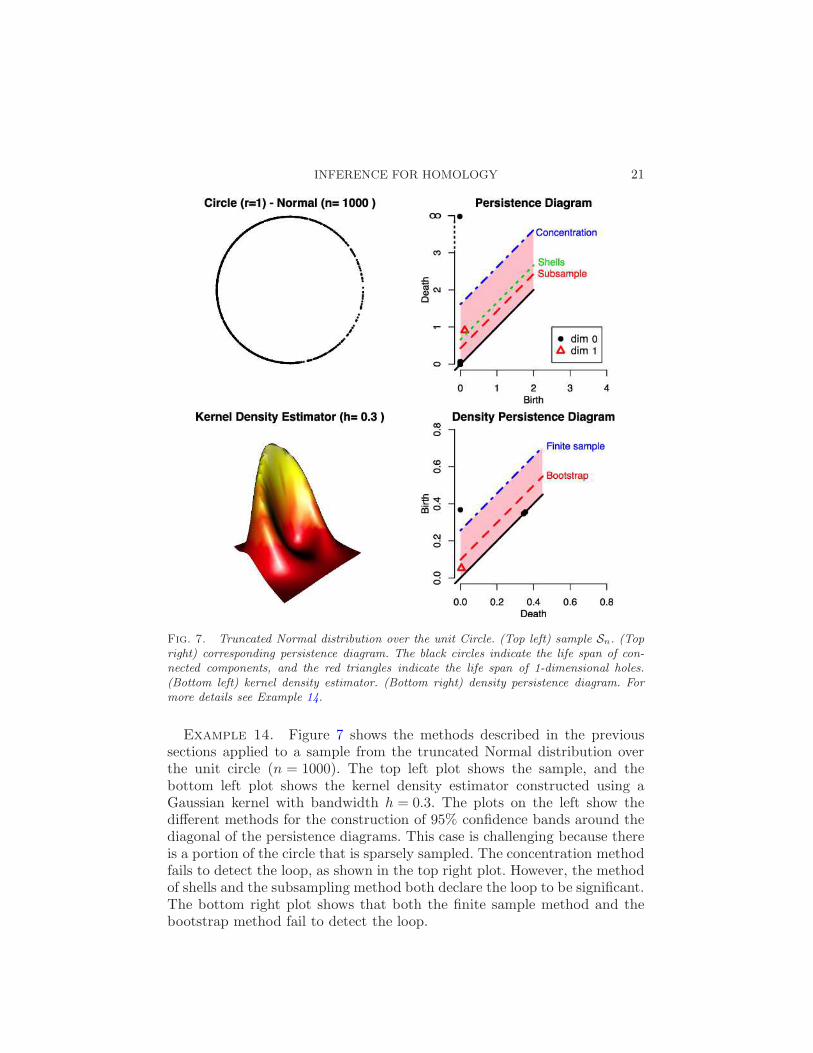
Fig. 7. Truncated Normal distribution over the unit Circle. (Top left) sample Sn. (Topright) corresponding persistence diagram. The black circles indicate the life span of con-nected components, and the red triangles indicate the life span of 1-dimensional holes.(Bottom left) kernel density estimator. (Bottom right) density persistence diagram. Formore details see Example 14.

Example 14. Figure 7 shows the methods described in the previoussections applied to a sample from the truncated Normal distribution overthe unit circle (n = 1000). The top left plot shows the sample, and thebottom left plot shows the kernel density estimator constructed using aGaussian kernel with bandwidth h = 0.3. The plots on the left show thedifferent methods for the construction of 95% confidence bands around thediagonal of the persistence diagrams. This case is challenging because thereis a portion of the circle that is sparsely sampled. The concentration methodfails to detect the loop, as shown in the top right plot. However, the methodof shells and the subsampling method both declare the loop to be significant.The bottom right plot shows that both the finite sample method and thebootstrap method fail to detect the loop.


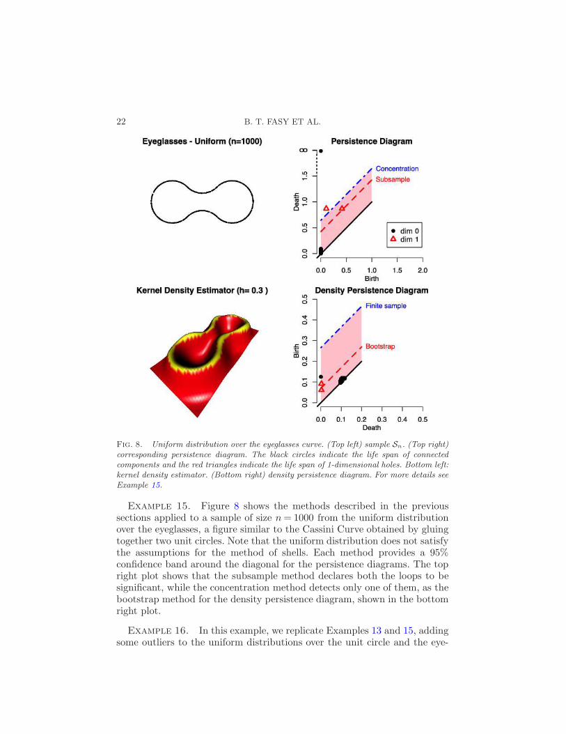
Fig. 8. Uniform distribution over the eyeglasses curve. (Top left) sample Sn. (Top right)corresponding persistence diagram. The black circles indicate the life span of connectedcomponents and the red triangles indicate the life span of 1-dimensional holes. Bottom left:kernel density estimator. (Bottom right) density persistence diagram. For more details seeExample 15.

Example 15. Figure 8 shows the methods described in the previoussections applied to a sample of size n= 1000 from the uniform distributionover the eyeglasses, a figure similar to the Cassini Curve obtained by gluingtogether two unit circles. Note that the uniform distribution does not satisfythe assumptions for the method of shells. Each method provides a 95%confidence band around the diagonal for the persistence diagrams. The topright plot shows that the subsample method declares both the loops to besignificant, while the concentration method detects only one of them, as thebootstrap method for the density persistence diagram, shown in the bottomright plot.

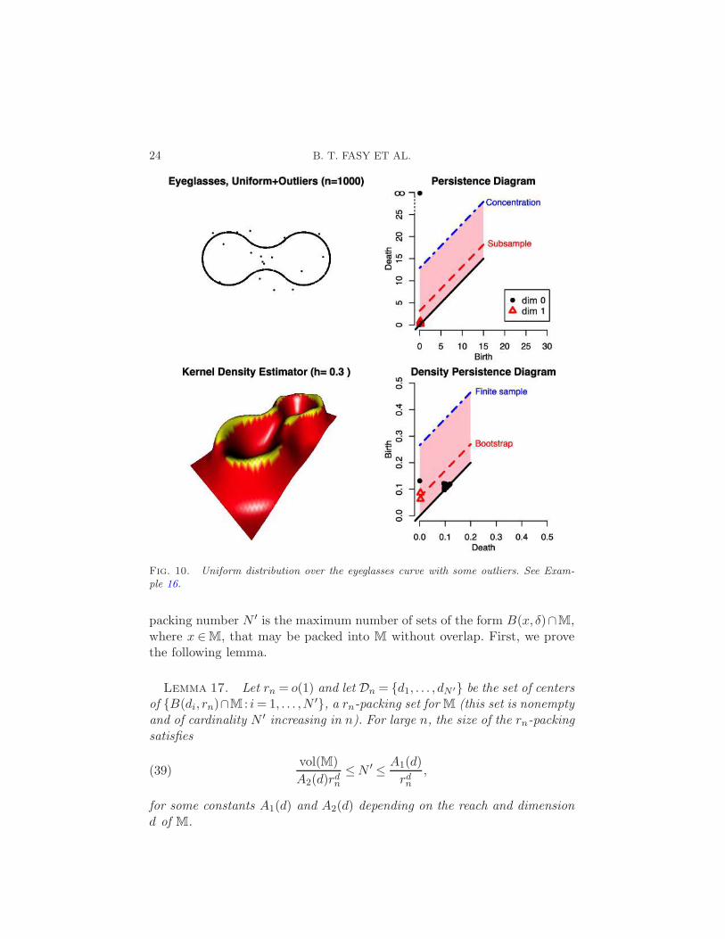
Example 16. In this example, we replicate Examples 13 and 15, addingsome outliers to the uniform distributions over the unit circle and the eye-


Fig. 9. Uniform distribution over the unit Circle with some outliers. See Example 16.

glasses. Figures 9 and 10 show the persistence diagrams with different meth-ods for the construction of 95% confidence bands. Much of the literature oncomputational topology focuses on methods that use the distance functionto the data. As we see here, and as discussed in Bendich, Galkovskyi andHarer (2011), such methods are quite fragile. A few outliers are sufficientto drastically change the persistence diagram and force the concentrationmethod and the subsample method to declare the topological features tobe not significant. On the other hand the density-based methods are veryinsensitive to the presence of outliers, as shown in the bottom right plots ofthe two figures.

6. Proofs. In this section, we provide proofs of the theorems and lemmasfound in Section 3.

Recall that the δ-covering number N of a manifold M is the smallestnumber of Euclidean balls of radius δ required to cover the set. The δ-


Fig. 10. Uniform distribution over the eyeglasses curve with some outliers. See Exam-ple 16.

packing number N ′ is the maximum number of sets of the form B(x, δ)∩M,where x ∈M, that may be packed into M without overlap. First, we provethe following lemma.

Lemma 17. Let rn = o(1) and let Dn = d1, . . . , dN ′ be the set of centersof B(di, rn)∩M : i= 1, . . . ,N ′, a rn-packing set for M (this set is nonemptyand of cardinality N ′ increasing in n). For large n, the size of the rn-packingsatisfies

vol(M)

A2(d)rdn≤N ′ ≤ A1(d)

rdn,(39)

for some constants A1(d) and A2(d) depending on the reach and dimensiond of M.


Proof. From the proof of Lemma 4 we know that

N ′ ≤ A1(d)

rdn,(40)

where A1(d) is a constant depending on the dimension of the manifold.A similar lower bound for N ′ can be obtained. Let N be the size of a2rn-covering set for M, formed by Euclidean balls B(ci,2rn) with centersC = c1, . . . , cN. By Lemma 5.2 in Niyogi, Smale and Weinberger (2008)and a simple volume argument we have

N ′ ≥N ≥ vol(M)

maxi=1,...,N vol(B(ci,2rn)∩M).(41)

For large n, by Corollary 1.3 in Chazal (2013),

maxi=1,...,N

vol(B(ci,2rn)∩M)≤A2(d)rdn,(42)

where A2(d) is a constant depending on the dimension of the manifold.Combining (40), (41) and (42) we obtain (39).

Proof of Theorem 3. We begin the proof by showing that thereexists an event of probability approaching one (as n→∞) such that, overthis event, for any subsample Sb,n of the data Sn of size b,

H(Sn,M)≤H(Sb,n,Sn).(43)

Toward this end, let tn = (4ρlognn )1/d, and define the event An = H(Sn,M)<

tn. Then, by the remark following Lemma 4, P(Acn)≤ 2d−1

n logn , for all n large

enough. Next, let Dn = d1, . . . , dN ′ be the set of centers of B(di,2tn) ∩M : i= 1, . . . ,N ′, a 2tn-packing set for M. By Lemma 17, the size of Dn isof order t−d

n =Θ( nlogn).

We can now show (43). Suppose An holds and, arguing by contradiction,also that H(Sb,n,Sn)<H(Sn,M). Then

H(Sb,n,Dn)≤H(Sb,n,Sn) +H(Sn,Dn)<H(Sn,M) +H(Sn,D)

≤ 2H(Sn,M)(44)

≤ 2tn.

Because of our assumption on b and of (39), bN ′ → 0 as n→∞, which implies

that a (1 − o(1)) fraction of the balls B(dj ,2tn), j = 1, . . . ,N ′ containsno points from Sb,n. So H(Sb,n,D) > 2tn, which, in light of (44), yields acontradiction. Thus, on An, (43) holds, for any subsample Sb,n of size b, asclaimed.


Next, let Sjb,n, j = 1, . . . ,N be an enumeration of all possible subsamples

of Sn of size b, where N =(nb

), and define

Lb(t) =1

N

N∑

j=1

I(H(Sjb,n,M)> t).

Using (43) we obtain that, on the event An,

H(Sjb ,M)≤H(Sj

b ,Sn) +H(Sn,M)≤ 2H(Sjb ,Sn),

and therefore, H(Sjb ,Sn)≥H(Sj

b ,M)/2, simultaneously over all j = 1, . . . ,N .Thus, on that event

Lb(t)≤ Lb(t/2) for all t > 0,(45)

where Lb is defined in (13). Thus, letting 1An = 1An(Sn) be the indicatorfunction of the event An, we obtain the bound

Lb(cb) = Lb(cb)(1An + 1Acn)≤Lb(cb/2) + 1Ac

n≤ α+ 1Ac

n,

where the first inequality is due to (45) and the second inequality to the factthat Lb(cb/2) = α, by definition of cb. Taking expectations, we obtain that

E(Lb(cb))≤ α+ P(Acn) = α+O

(1

n logn

).(46)

Next, define

Jb(t) = P(H(Sb,M)> t), t > 0,

where we recall that Sb is an i.i.d. sample of size b. Then Lemma A.2 inRomano and Shaikh (2012) yields that, for any ǫ > 0,

P

(supt>0

|Lb(t)− Jb(t)|> ǫ)≤ 1

ǫ

√2π

kn,(47)

where kn = ⌊nb ⌋. Let Bn be the event that

supt>0

|Lb(t)− Jb(t)| ≤√2π

k1/4n

and 1Bn = 1Bn(Sn) be its indicator function. Then

E

(supt>0

|Lb(t)− Jb(t)|1Bn

)≤

√2π

k1/4n

,

and, using (47) and the fact that supt |Lb(t)− Jb(t)| ≤ 1 almost everywhere,

E

(supt>0

|Lb(t)− Jb(t)|1Bcn

)≤ P(Bc

n)≤1

k1/4n

.


Thus

E

(supt>0

|Lb(t)− Jb(t)|)=O

(1

k1/4n

)=O

(b

n

)1/4

.(48)

We can now prove the claim of the theorem. First notice that the followingbounds hold:

P(H(Sn,M)> cb)≤ P(H(Sb,M)> cb)

= Jb(cb)

≤ Lb(cb) + supt>0

|Lb(t)− Jb(t)|.

Now take expectations on both sides, and use (46) and (48) to obtain that

P(H(Sn,M)> cb)≤O

(b

n

)1/4

+O

(1

n logn

)=O

(b

n

)1/4

,

as claimed.

Proof of Lemma 4. Let C = c1, . . . , cN be the set of centers of Eu-clidean balls B1, . . . ,BN, forming a minimal t/2-covering set for M, fort/2< diam(M). Then H(C,M)≤ t/2 and

P(H(Sn,M)> t)≤ P(H(Sn,C) +H(C,M)> t)

≤ P(H(Sn,C)> t/2)

= P(Bj ∩ Sn =∅ for some j)

≤∑

j

P (Bj ∩ Sn =∅)

=∑

j

[1− P (Bj)]n

≤N [1− ρ(t)td]n

≤N exp(−nρ(t)td),

where the second-to-last inequality follows from the fact that minj P (Bj)≥ρ(t)td by definition of ρ(t) and the last inequality from the fact that ρ(t)td ≤1. Next, let D = d1, . . . , dN ′ be the set of centers of B′

1∩M, . . . ,B′N ′ ∩M,

a maximal t/4-packing set for M. Then N ≤N ′ [see, e.g., Lemma 5.2, Niyogi,Smale and Weinberger (2008), for a proof of this standard fact], and bydefinition, the balls B′

j ∩M, j = 1, . . . ,N ′ are disjoint. Therefore,

1 = P (M)≥N ′∑

j=1

P (B′j ∩M) =

N ′∑

j=1

P (B′j)≥N ′ρ(t/2)

td

2d,


where we have used again the fact that minj P (B′j)≥ ρ(t/2) t

d

2d. We conclude

that N ≤N ′ ≤ (2d)/(ρ(t/2)td). Hence

P(H(Sn,M)> t)≤ 2d

ρ(t/2)tdexp(−nρ(t)td).

Now suppose that t <minρ/(2C2), t0 (C2 and t0 are defined in Assump-tion A2). Then, since we assume that ρ(t) is differentiable on [0, t0] withderivative bounded in absolute value by C2, there exists a 0 ≤ t ≤ t suchthat

ρ(t) = ρ+ tρ′(t)≥ ρ−C2t≥ρ

2.

Similarly, under the same conditions on t, we have that ρ(t/2) ≥ ρ2 . The

result follows.

Proof of Theorem 5. Let

ρ(x, t) =Pn(B(x, t/2))

td.

Note that

supx∈M

P (B(x, rn/2))≤Crdn(49)

for some C > 0, since ρ(x, t) is bounded by Assumption A2. Let rn =

( lognn )1/(d+2) , and consider all n large enough so that

ρ

2(logn)d/(d+2) > 1 and n2/(d+2) − 2

d+ 2logn> 0.(50)

Let E1,n be the event that the sample Sn forms an rn-cover for M. Then, byLemma 4 and since P(Ec

1,n) = P(H(Sn,M)≤ rn), we have

P(Ec1,n)≤

2d+1

ρ

(n

logn

)d/(d+2)

exp

−ρ

2n

(logn

n

)d/(d+2)

≤ 2d+1

ρnd/(d+2) exp

−(ρ

2(logn)d/(d+2)

)n2/(d+2)

≤ 2d+1

ρnd/(d+2) exp−n2/(d+2)

≤ 2d+1

ρexp

−n2/(d+2) +

d

d+2logn

≤ 2d+1

ρ

1

n,


where the third and last inequalities hold since n is assumed large enoughto satisfy (50).

Let C3 =maxC1,C2 where C1 and C2 are defined in Assumption A2.Let

ǫn =

√C

2 logn

(n− 1)rdn

with C =max4C3,2(C+1/3), for some C satisfying (49). Assume furtherthat n is large enough so that, in addition to (50), ǫn < 1. With this choiceof ǫn, define the event

E2,n =

max

i=1,...,n

∣∣∣∣Pi,n−1(B(Xi, rn/2))

rdn− P (B(Xi, rn/2))

rdn

∣∣∣∣≤ c∗ǫn

,

where Pi,n−1 is the empirical measure corresponding to the data points Sn \Xi, and c∗ is a positive number satisfying

c∗ǫnrdn −

1

n≥ ǫnr

dn

for all n large enough (which exists by our choice of ǫn and rn). We will showthat P(E2,n)≥ 1− 2

n . To this end, let Pi denote the probability induced by

Sn \ Xi (which, by independence is also the conditional probability of Sn

given Xi) and Pi be the marginal probability induced by Xi, for i= 1, . . . , n.Then

P(Ec2,n)≤

n∑

i=1

P

(∣∣∣∣Pn(B(Xi, rn/2))

rdn− P (B(Xi, rn/2))

rdn

∣∣∣∣> c∗ǫn

)

≤n∑

i=1

P

(|Pi,n−1(B(Xi, rn/2))−P (B(Xi, rn/2))|> c∗ǫnr

dn −

1

n

)

(51)

≤n∑

i=1

P(|Pi,n−1(B(Xi, rn/2))−P (B(Xi, rn/2))|> ǫnrdn)

=

n∑

i=1

Ei[Pi(|Pi,n−1(B(Xi, rn/2))− P (B(Xi, rn/2))|> ǫnr

dn)],

where the first inequality follows from the union bound, the second fromthe fact that |Pn(B(Xi, rn/2)) − Pi,n−1(B(Xi, rn/2))| ≤ 1

n for all i (almost

everywhere with respect to the join distribution of the sample) and the thirdinequality from the definition of c∗.

By Bernstein’s inequality, for any i= 1, . . . , n,

Pi(|Pi,n−1(B(Xi, rn/2))−P (B(Xi, rn/2))|> ǫnr

dn)


≤ 2exp

−1

2

(n− 1)ǫ2nr2dn

Crdn + 1/3rdnǫn

≤ 2exp

−1

2

(n− 1)ǫ2nrdn

(C +1/3)

≤ 2

n2,

where in the first inequality we have used the fact that P (B(x, rn/2))(1 −P (B(x, rn/2)))≤Crdn. Therefore, from (51),

P(Ec2,n)≤

2

n.

Let j = argmini ρ(Xi, rn) and k = argmini ρ(Xi, rn). Suppose E2,n holdsand, arguing by contradiction, that

|ρ(Xj , rn)− ρ(Xk, rn)|= |ρn − ρ(Xk, rn)|> c∗ǫn.(52)

Since E2,n holds, we have |ρ(Xj , rn) − ρ(Xj , rn)| ≤ c∗ǫn and |ρ(Xk, rn) −ρ(Xk, rn)| ≤ c∗ǫn. This implies that if ρ(Xj , rn)< ρ(Xk, rn), then ρ(Xj , rn)<ρ(Xk, rn), while if ρ(Xj , rn) > ρ(Xk, rn), then ρ(Xk, rn) < ρ(Xj , rn), whichis a contradiction.

Therefore, with probability P(E1,n ∩ E2,n) ≥ 1 − (2d+1/ρ)+2n , the sample

points Sn forms an rn-covering of M and∣∣∣ρn −min

iρ(Xi, rn)

∣∣∣≤ c∗ǫn.

Since the sample Sn is a covering of M,∣∣∣min

iρ(Xi, rn)− inf

x∈Mρ(x, rn)

∣∣∣≤maxi

supx∈B(Xi,rn)

|ρ(x, rn)− ρ(Xi, rn)|.(53)

Because ρ(x, t) has a bounded continuous derivative in t uniformly over x,we have, if rn < t0,

supx∈B(Xi,rn)

|ρ(x, rn)− ρ(Xi, rn)| ≤C3rn,

almost surely. Furthermore, since ρ(t) is right-differentiable at zero,

|ρ(rn)− ρ| ≤C3rn,

for all rn < t0. Combining the last two observations with (53) and using thetriangle inequality, we conclude that

|ρn − ρ| ≤ c∗ǫn + 2C3rn,


with probability at least 1− (2d+1/ρ)+2n , for all n large enough. Because our

choice of rn satisfies the equation ǫn = Θ(√

lognnrdn

), the terms on the right-

hand side of the last display are balanced, so that

|ρn − ρ| ≤C4

(logn

n

)1/(d+2)

,

for some C4 > 0.

Proof of Theorem 6. Let P1 denote the unconditional probabilitymeasure induced by the first random half S1,n of the sample, P2 the con-ditional probability measure induced by the second half of the sample S2,n

given the outcome of the data splitting and the values of the first sample, andP1,2 the probability measure induced by the whole sample and the randomsplitting. Then

P(H(S2,n,M)> t1,n) = P1,2(H(S2,n,M)> t1,n) = E1(P2(H(S2,n,M)> t1,n)),

where E1 denotes the expectation corresponding to P1. By Theorem 5,there exist constants C and C ′ such that the event An that |ρ1,n − ρ| ≤C( lognn )1/(d+2) has P1-probability no smaller than 1− C′

n , for n large enough.Then

E1(P2(H(S2,n,M)> t1,n))(54)

≤ E1(P2(H(S2,n,M)> t1,n);An) + P1(Acn),

where, for a random variable X with expectation EX and an event E measur-able with respect to X , we write E[X;E ] for the expectation of X restrictedto the sample points in E .

Define F (t, ρ) = 2d+1

tdρe−((ρn)/2)td . Then, by Lemma 4,

P2(H(S2,n,M)> t1,n)≤ F (t1,n, ρ).

The rest of the proof is devoted to showing that, on An, F (t1,n, ρ) ≤ α+

O((logn/2)1/(d+2)). To simplify the derivation, we will write O(Rn) to in-dicate a term that is in absolute value of order O((logn/n)1/(d+2)), wherethe exact value of the constant may change from line to line. Accordingly,on the event An and for n large enough, ρ1,n − ρ=O(Rn). Since ρ > 0 byassumption, this implies that, on the same event and for n large,

ρ1,nρ

= 1+O(Rn) andρ

ρ1,n= 1+O(Rn).


Now, on An and for all n large enough,

F (t1,n, ρ) =2d+1

td1,nρexp

(−ntd1,nρ

2

)

=

(ρ1,nρ

)2d+1

td1,nρ1,nexp

(−ntd1,nρ1,n(ρ/ρ1,n)

2

)

= (1+O(Rn))F (t1,n, ρ1,n) exp

(−ntd1,nρ1,nO(Rn)

2

)(55)

= α(1 +O(Rn))

[exp

(−ntd1,nρ1,n

2

)]O(Rn)

= α(1 +O(Rn))

[α

2td1,nρ1,n

]O(Rn)

,

where the last two identities follow from the fact that

F (t1,n, ρ1,n) = α(56)

for all n.Next, let t∗n = ( 2

αρlognn )1/d. We then claim that, for all n large enough and

on the event An, t1,n ≤ t∗n. In fact, using similar arguments,

F (t∗n, ρ1,n) = F (t∗n, ρ)(1 +O(Rn)) exp(−nt∗nO(Rn))→ 0 as n→∞,

since O(Rn) = o(1) and, by Lemma 4, F (t∗n, ρ)→ 0 and n→∞.By (56), it then follows that, for all n large enough, F (t1,n, ρ1,n) >

F (t∗n, ρ1,n). Because F (t, ρ) is decreasing in t for each ρ, the claim is proved.Thus, substituting t1,n with t∗n in equation (55) yields

F (t1,n, ρ)≤ F (t∗n, ρ)

≤ α(1 +O(Rn))

[α

2(t∗n)

dρ1,n

]O(Rn)

= α(1 +O(Rn))

[α

2(t∗n)

dρ(1 +O(Rn))

]O(Rn)

= α(1 +O(Rn))

[logn

n+ o(1)

]O(Rn)

= α(1 +O(Rn))(1 + o(1))

= α+O(Rn),


as n→∞, where we have written as o(1) all terms that are lower order thanO(Rn). The second-to-last step follows from the limit

limn→∞

(logn

n

)O(Rn)

= limn→∞

exp

log

(logn

n

)C

(logn

n

)1/(d+2)

= exp

limn→∞

log

(logn

n

)C

(logn

n

)1/(d+2)= 1,

for some constant C.Therefore, on the event An and for all n large enough,

P2(H(S2,n,M)> t1,n)≤ α+O(Rn).

Since P1(An) =O(Rn) [in fact, it is of lower order than O(Rn)], the resultfollows from (54).

Proof of Theorem 7. Let B = supx∈M ρ(x,↓ 0). Fix some δ ∈ (0,B−ρ). Choose equally spaced values ρ ≡ γ1 < γ2 < · · · < γm < γm+1 ≡ B suchthat δ ≥ γj+1−γj. Let Ωj = x :γj ≤ ρ(x,↓ 0)< γj+1, and define h(Sn,Ωj) =supy∈Ωj

minx∈Sn ‖x − y‖2 for j = 1, . . . ,m. Now H(Sn,M) = h(Sn,M) ≤maxj h(Sn,Ωj), and so

P(H(Sn,M)> t)≤ P

(max

jh(Sn,Ωj)> t

)≤

m∑

j=1

P(h(Sn,Ωj)> t).

Let Cj = cj1, . . . , cjNj be the set of centers of B(cj1, t/2), . . . ,B(cjNj

, t/2),a t/2-covering set for Ωj , for j = 1, . . . ,m. Let Bjk = B(cjk, t/2), for k =1, . . . ,Nj . Then, for all j and for t <minγj/(2C1), t0 (C1 and t0 are de-fined in Assumption A2), there is 0≤ t≤ t such that

P (Bjk)

td= ρ(cjk, t)≥ ρ(cjk,↓ 0) + tρ′(cjk(t))≥ ρ(cjk,↓ 0)−C1t≥

γj2

and

P(h(Sn,Ωj)> t)≤ P(h(Sn,Cj) + h(Cj ,Ωj)> t)

≤ P(h(Sn,Cj)> t/2)

≤ P(Bjk ∩ Sn =∅ for some k)

≤Nj∑

k=1

P(Bjk ∩ Sn =∅)

≤Nj∑

k=1

[1− P (Bjk)]n ≤

Nj∑

k=1

[1− td

γj2

]n

=Nj

[1− td

γj2

]n≤Nj exp

(−nγjt

d

2

).


Following the strategy in the proof of Lemma 4,

P (Ωj)≥∑

k

P (Bjk)≥Njtd γj2d+1

,

so that Nj ≤ 2d+1P (Ωj)/(γjtd). Therefore, for t <minρ/(2C1), t0,

P(H(Sn,M)> t) ≤ 2d+1

td

m∑

j=1

P (Ωj)

γjexp

(−nγjt

d

2

)

=2d+1

td

m∑

j=1

G(γj + δ)−G(γj)

δ

δ

γjexp

(−nγjt

d

2

)

→ 2d+1

td

∫ B

ρ

g(v)

vexp

(−nvtd

2

)dv

as δ→ 0.

Proof of Theorem 8. Let

g∗(v) =1

n

n∑

i=1

1

bK

(v−Wi

b

),(57)

where Wi = ρ(Xi,↓ 0). Thensupv|g(v)− g(v)| ≤ sup

v|g(v)− g∗(v)|+ sup

v|g∗(v)− g(v)|.

By standard asymptotics for kernel estimators,

supv|g(v)− g∗(v)| ≤C1b

2 +OP

(√logn

nb

).

Next, note that∣∣∣∣K

(v−Wi

b

)−K

(v− Vi

b

)∣∣∣∣≤C|Wi − Vi|

b rn

b(58)

from Theorem 5. Hence,

|g∗(v)− g(v)| rnb2

.

Statement (1) follows.To show the second statement, we will use the same notation and a similar

strategy as in the proof of Theorem 6. Thus

P(H(S2,n,M)> t1,n) = P1,2(H(S2,n,M)> t1,n)

= E1(P2(H(S2,n,M)> t1,n)).


Let An be the event defined in the proof of Theorem 6 and Bn the eventthat supv |g(v)− g(v)| ≤ rn. Then P1(An ∩Bn)≥ 1−O(1/n). Now,

E1(P2(H(S2,n,M)> t1,n))

≤ E1(P2(H(S2,n,M)> t1,n);An ∩ Bn) + P1((An ∩Bn)c).

By Theorem 7, conditionally on S1,n and the randomness of the data split-ting,

P2(H(S2,n,M)> t1,n)≤2d+1

td1,n

∫ ∞

ρ

g(v)

ve−nv(td1,n/2) dv.(59)

We will show next that, on the event An ∩ Bn, the right-hand side of theprevious equation is bounded by α+O(rn) as n→∞. The second claim ofthe theorem will then follow. Throughout the proof, we will assume that theevent An ∩ Bn holds.

Recall that t1,n solves the equation

2d+1

td1,n

∫ ∞

ρ

g(v)

ve−nv(td1,n/2) dv = α(60)

(and this solution exists for all large n). By assumption, g(v) is uniformlybounded away from 0. Hence g(v)/g(v) = 1+O(rn) and so

2d+1

td1,n

∫ ∞

ρ

g(v)

ve−nv(td1,n/2) dv

=2d+1

td1,n

∫ B

ρn

g(v)

ve−nv(td1,n/2) dv+ zn

= (1 +O(rn))2d+1

td1,n

∫ B

ρn

g(v)

ve−nv(td1,n/2) dv+ zn

= α(1 +O(rn)) +O(ρn − ρ) + zn

= α+O(rn) + zn,

where

zn =2d+1

td1,n

∫ ρn

ρ

g(v)

ve−nv(td1,n/2) dv.

Now t1,n ≥ c1(logn/n)1/d ≡ un for some c > 0, for all large n since otherwise

the left-hand side of (60) would go to zero, and (60) would not be satisfied.So, for some positive c2, c3,

zn ≤ 2d+1

udn

∫ ρn

ρ

g(v)

ρe−nρ(ud

n/2) dv ≤ |ρn − ρ| c2nc3

=O(|ρn − ρ|).


Proof of Lemma 9. First we show that

|ph(x)− ph(y)| ≤L

hD+1‖x− y‖2.

This follows from the definition of ph,

|ph(x)− ph(y)|

=

∣∣∣∣1

hD

∫

XK

(‖x− u‖h

)dP (u)− 1

hD

∫

XK

(‖y − u‖h

)dP (u)

∣∣∣∣

≤ 1

hD

∫

X

∣∣∣∣K(‖x− u‖

h

)−K

(‖y − u‖h

)∣∣∣∣dP (u)

≤ 1

hD

∫

XL

∣∣∣∣‖x− u‖

h− ‖y − u‖

h

∣∣∣∣dP (u)

≤ L

hD‖x− y‖

h=

L

hD+1‖x− y‖.

By a similar argument,

|ph(x)− ph(y)| ≤L

hD+1‖x− y‖.

Divide X into a grid based on cubes A1, . . . ,AN with length of size ε. Notethat N ≍ (C/ε)D . Each cube Aj has diameter

√Dε. Let cj be the center of

Aj . Now

‖ph − ph‖∞ = supx|ph(x)− ph(x)|=max

jsupx∈Aj

|ph(x)− ph(x)|

≤(max

j|ph(cj)− ph(cj)|

)+2v,

where v = Lε√D

2hD+1 . We have that

P(‖ph − ph‖∞ > δ)≤ P

(max

j|ph(cj)− ph(cj)|> δ − 2v

)

≤∑

j

P(|ph(cj)− ph(cj)|> δ − 2v).

Let ε= δhD+1

2L√D. Then 2v = δ/2, and so

P(‖ph − ph‖∞ > δ)≤∑

j

P

(|ph(cj)− ph(cj)|>

δ

2

).

Note that ph(x) is an average of quantities bounded between zero andK(0)/(nhD). Hence, by Hoeffding’s inequality,

P

(|ph(cj)− ph(cj)|>

δ

2

)≤ 2exp

(−nδ2h2D

2K2(0)

).


Therefore, summing over j, we conclude

P(‖ph − ph‖∞ > δ)≤ 2N exp

(−nδ2h2D

2K2(0)

)

= 2

(C

ε

)D

exp

(−nδ2h2D

2K2(0)

)

= 2

(4CL

√D

δhD+1

)D

exp

(−nδ2h2D

2K2(0)

).

7. Conclusion. We have presented several methods for separating noisefrom signal in persistent homology. The first three methods are based on thedistance function to the data. The last uses density estimation. There is auseful analogy here: methods that use the distance function to the data arelike statistical methods that use the empirical distribution function. Methodsthat use density estimation use smoothing. The advantage of the former isthat it is more directly connected to the raw data. The advantage of thelatter is that it is less fragile; that is, it is more robust to noise and outliers.

We conclude by mentioning some open questions that we plan to addressin future work:

(1) We focus on assessing the uncertainty of persistence diagrams. Simi-lar ideas can be applied to assess uncertainty in barcode plots. This requiresassessing uncertainty at different scales ε. This suggests examining the vari-ability of H(Sε, Sε) at different values of ε. From Molchanov (1998), we havethat

√nεDH(Sε, Sε) inf

x∈∂Sε

∣∣∣∣G(x)

L(x)

∣∣∣∣,(61)

where G is a Gaussian process,

L(x) =d

dtinfpε(y)− pε(x) :‖x− y‖ ≤ t

∣∣∣t=0

(62)

and pǫ(x) is the mean of the kernel estimator using a spherical kernel withbandwidth ε. The limiting distribution it is not helpful for inference becauseit would be very difficult to estimate L(x). We are investigating practical

methods for constructing confidence intervals on H(Sε, Sε) and using thisto assess uncertainty of the barcodes.

(2) Confidence intervals provide protection against type I errors, that is,false detections. It is also important to investigate the power of the methodsto detect real topological features. Similarly, we would like to quantify theminimax bounds for persistent homology.

(3) In the density estimation method, we use a fixed bandwidth. Spatiallyadaptive bandwidths might be useful for more refined inferences.


(4) It is also of interest to construct confidence intervals for other topo-logical parameters such as the degree p total persistence defined by

θ = 2∑

d(x,Diag)p,

where the sum is over the points in P whose distance from the diagonal isgreater than some threshold, and Diag denotes the diagonal.

(5) Our experiments are meant to be a proof of concept. Detailed simu-

lation studies are needed to see under which conditions the various methodswork well.

(6) The subsampling method is very conservative due to the fact that b=o(n). Essentially, there is a bias of orderH(Sb,M)−H(Sn,M). We conjecture

that it is possible to adjust for this bias.(7) The optimal bandwidth for the density estimation method is an open

question. The usual theory is based on L2 loss which is not necessarilyappropriate for topological estimation.

Acknowledgments. The authors would like to thank the anonymous re-

viewers for their suggestions and feedback, as well as Frederic Chazal andPeter Landweber for their comments.

SUPPLEMENTARY MATERIAL

Supplement to “Confidence sets for persistence diagrams”

(DOI: 10.1214/14-AOS1252SUPP; .pdf). In the supplementary material wegive a brief introduction to persistence homology and provide additional

details about homology, simplicial complexes and stability of persistencediagrams.

REFERENCES

Ambrosio, L., Fusco, N. and Pallara, D. (2000). Functions of Bounded Variation and

Free Discontinuity Problems. Oxford Mathematical Monographs. Clarendon Press, NewYork. MR1857292

Balakrishnan, S., Rinaldo, A., Sheehy, D., Singh, A. and Wasserman, L. (2011).Minimax rates for homology inference. Preprint. Available at arXiv:1112.5627.

Bendich, P., Galkovskyi, T. and Harer, J. (2011). Improving homology estimateswith random walks. Inverse Problems 27 124002. MR2854318

Bendich, P., Mukherjee, S. and Wang, B. (2010). Towards stratification learningthrough homology inference. Preprint. Available at arXiv:1008.3572.

Blumberg, A. J.,Gal, I., Mandell, M. A. and Pancia, M. (2012). Persistent homologyfor metric measure spaces, and robust statistics for hypothesis testing and confidence

intervals. Preprint. Available at arXiv:1206.4581.

http://dx.doi.org/10.1214/14-AOS1252SUPP

http://www.ams.org/mathscinet-getitem?mr=1857292

http://arxiv.org/abs/arXiv:1112.5627





Bubenik, P. and Kim, P. T. (2007). A statistical approach to persistent homology. Ho-mology, Homotopy Appl. 9 337–362. MR2366953

Bubenik, P., Carlsson, G., Kim, P. T. and Luo, Z.-M. (2010). Statistical topologyvia Morse theory persistence and nonparametric estimation. In Algebraic Methods inStatistics and Probability II. Contemp. Math. 516 75–92. Amer. Math. Soc., Providence,

RI. MR2730741Carlsson, G. (2009). Topology and data. Bull. Amer. Math. Soc. (N.S.) 46 255–308.

MR2476414Carlsson, G. and Zomorodian, A. (2009). The theory of multidimensional persistence.

Discrete Comput. Geom. 42 71–93. MR2506738

Chazal, F. (2013). An upper bound for the volume of geodesic balls in submanifolds ofEuclidean spaces. Technical report, INRIA.

Chazal, F. and Oudot, S. Y. (2008). Towards persistence-based reconstruction inEuclidean spaces. In Computational Geometry (SCG’08) 232–241. ACM, New York.MR2504289

Chazal, F., Cohen-Steiner, D., Merigot, Q. et al. (2010). Geometric inference formeasures based on distance functions. INRIA RR–6930.

Chazal, F., Oudot, S., Skraba, P. and Guibas, L. J. (2011). Persistence-based clus-tering in Riemannian manifolds. In Computational Geometry (SCG’11) 97–106. ACM,New York. MR2919600

Chazal, F., de Silva, V., Glisse, M. and Oudot, S. (2012). The structure and stabilityof persistence modules. Preprint. Available at arXiv:1207.3674.

Chazal, F., Fasy, B. T., Lecci, F., Rinaldo, A., Singh, A. and Wasserman, L.

(2013a). On the bootstrap for persistence diagrams and landscapes. Preprint. Availableat arXiv:1311.0376.

Chazal, F., Glisse, M., Labruere, C. and Michel, B. (2013b). Optimal rates of con-vergence for persistence diagrams in topological data analysis. Preprint. Available at

arXiv:1305.6239.Cohen-Steiner, D., Edelsbrunner, H. and Harer, J. (2007). Stability of persistence

diagrams. Discrete Comput. Geom. 37 103–120. MR2279866

Cohen-Steiner, D., Edelsbrunner, H., Harer, J. and Mileyko, Y. (2010). Lipschitzfunctions have Lp-stable persistence. Found. Comput. Math. 10 127–139. MR2594441

Cuevas, A. (2009). Set estimation: Another bridge between statistics and geometry. Bol.Estad. Investig. Oper. 25 71–85. MR2750781

Cuevas, A., Febrero, M. and Fraiman, R. (2001). Cluster analysis: A further approach

based on density estimation. Comput. Statist. Data Anal. 36 441–459. MR1855727Cuevas, A. and Fraiman, R. (1997). A plug-in approach to support estimation. Ann.

Statist. 25 2300–2312. MR1604449Cuevas, A. and Fraiman, R. (1998). On visual distances in density estimation: The

Hausdorff choice. Statist. Probab. Lett. 40 333–341. MR1664548

Cuevas, A., Fraiman, R. and Pateiro-Lopez, B. (2012). On statistical properties ofsets fulfilling rolling-type conditions. Adv. in Appl. Probab. 44 311–329. MR2977397

Cuevas, A. and Rodrıguez-Casal, A. (2004). On boundary estimation. Adv. in Appl.Probab. 36 340–354. MR2058139

Devroye, L. and Wise, G. L. (1980). Detection of abnormal behavior via nonparametric

estimation of the support. SIAM J. Appl. Math. 38 480–488. MR0579432Edelsbrunner, H. and Harer, J. (2008). Persistent homology—a survey. In Surveys

on Discrete and Computational Geometry. Contemp. Math. 453 257–282. Amer. Math.Soc., Providence, RI. MR2405684





















Edelsbrunner, H. and Harer, J. L. (2010). Computational Topology: An Introduction.Amer. Math. Soc., Providence, RI. MR2572029

Fasy, B. T., Lecci, F., Rinaldo, A., Wasserman, L., Balakrishnan, S. andSingh, A. (2014). Supplement to “Confidence sets for persistence diagrams.”DOI:10.1214/14-AOS1252SUPP.

Federer, H. (1959). Curvature measures. Trans. Amer. Math. Soc. 93 418–491.MR0110078

Ghrist, R. (2008). Barcodes: The persistent topology of data. Bull. Amer. Math. Soc.(N.S.) 45 61–75. MR2358377

Gine, E. and Guillou, A. (2002). Rates of strong uniform consistency for multivari-

ate kernel density estimators. Ann. Inst. Henri Poincare Probab. Stat. 38 907–921.MR1955344

Hatcher, A. (2002). Algebraic Topology. Cambridge Univ. Press, Cambridge. MR1867354Heo, G., Gamble, J. and Kim, P. T. (2012). Topological analysis of variance and the

maxillary complex. J. Amer. Statist. Assoc. 107 477–492. MR2980059

Joshi, S., Kommaraju, R. V., Phillips, J. M. and Venkatasubramanian, S. (2011).Comparing distributions and shapes using the kernel distance. In Computational Ge-

ometry (SCG’11) 47–56. ACM, New York. MR2919594Kahle, M. (2009). Topology of random clique complexes. Discrete Math. 309 1658–1671.

MR2510573

Kahle, M. (2011). Random geometric complexes. Discrete Comput. Geom. 45 553–573.MR2770552

Kahle, M. and Meckes, E. (2013). Limit theorems for Betti numbers of random simpli-cial complexes. Homology, Homotopy Appl. 15 343–374. MR3079211

Lambert, J. H. (1758). Observationes variae in mathesin puram. Acta Helveticae Physico-

mathematico-anatomico-botanico-medica III 128–168.Mammen, E. and Tsybakov, A. B. (1995). Asymptotical minimax recovery of sets with

smooth boundaries. Ann. Statist. 23 502–524. MR1332579Mattila, P. (1995). Geometry of Sets and Measures in Euclidean Spaces: Fractals and

Rectifiability. Cambridge Studies in Advanced Mathematics 44. Cambridge Univ. Press,

Cambridge. MR1333890Mileyko, Y., Mukherjee, S. and Harer, J. (2011). Probability measures on the space

of persistence diagrams. Inverse Problems 27 124007, 22. MR2854323Molchanov, I. S. (1998). A limit theorem for solutions of inequalities. Scand. J. Stat.

25 235–242. MR1614288

Neumann, M. H. (1998). Strong approximation of density estimators from weakly depen-dent observations by density estimators from independent observations. Ann. Statist.

26 2014–2048. MR1673288Niyogi, P., Smale, S. and Weinberger, S. (2008). Finding the homology of submani-

folds with high confidence from random samples. Discrete Comput. Geom. 39 419–441.

MR2383768Niyogi, P., Smale, S. and Weinberger, S. (2011). A topological view of unsupervised

learning from noisy data. SIAM J. Comput. 40 646–663. MR2810909Penrose, M. (2003). Random Geometric Graphs. Oxford Studies in Probability 5. Oxford

Univ. Press, Oxford. MR1986198

Politis, D. N., Romano, J. P. and Wolf, M. (1999). Subsampling. Springer, New York.MR1707286

Romano, J. P. and Shaikh, A. M. (2012). On the uniform asymptotic validity of sub-sampling and the bootstrap. Ann. Statist. 40 2798–2822. MR3097960


http://dx.doi.org/10.1214/14-AOS1252SUPP





















Turner, K., Mileyko, Y., Mukherjee, S. and Harer, J. (2014). Frechet Means forDistributions of Persistence Diagrams. Discrete Comput. Geom. 52 44–70. MR3231030

B. T. Fasy

Computer Science Department

Tulane University

New Orleans, Louisiana 70118

USA

E-mail: [email protected]

F. Lecci

A. Rinaldo

L. Wasserman

Department of Statistics

Carnegie Mellon University

Pittsburgh, Pennsylvania 15213

USA

E-mail: [email protected]@[email protected]

S. Balakrishnan

A. Singh

Computer Science Department

Carnegie Mellon University

Pittsburgh, Pennsylvania 15213

USA

E-mail: [email protected]@cs.cmu.edu


mailto:[email protected]






confidence sets for persistence diagrams · confidence sets for persistence diagrams by brittany...

Documents