limit cycle walking, running, and skipping of the effect of high-speed telescopic-legs’ actuation....

Japan Advanced Institute of Science and Technology

JAIST Repositoryhttps://dspace.jaist.ac.jp/

TitleLimit cycle walking, running, and skipping of

telescopic-legged rimless wheel

Author(s) Asano, Fumihiko; Suguro, Masashi

Citation Robotica, 30(06): 989-1003

Issue Date 2011-11-29

Type Journal Article

Text version publisher

URL http://hdl.handle.net/10119/10845

Rights

Copyright (C) 2011 Cambridge University Press.

Fumihiko Asano and Masashi Suguro, Robotica,

30(06), 2011, 989-1003.

http://dx.doi.org/10.1017/S0263574711001226

Description

Roboticahttp://journals.cambridge.org/ROB

Additional services for Robotica:

Email alerts: Click hereSubscriptions: Click hereCommercial reprints: Click hereTerms of use : Click here

Limit cycle walking, running, and skipping of telescopiclegged rimless wheel

Fumihiko Asano and Masashi Suguro

Robotica / Volume 30 / Issue 06 / October 2012, pp 989 1003DOI: 10.1017/S0263574711001226, Published online:

Link to this article: http://journals.cambridge.org/abstract_S0263574711001226

How to cite this article:Fumihiko Asano and Masashi Suguro (2012). Limit cycle walking, running, and skipping of telescopiclegged rimless wheel. Robotica,30, pp 9891003 doi:10.1017/S0263574711001226

Request Permissions : Click here

Downloaded from http://journals.cambridge.org/ROB, IP address: 150.65.7.77 on 29 Aug 2012

Robotica (2012) volume 30, pp. 989–1003. © Cambridge University Press 2011doi:10.1017/S0263574711001226

Limit cycle walking, running, and skipping of telescopic-leggedrimless wheelFumihiko Asano∗ and Masashi SuguroSchool of Information Science, Japan Advanced Institute of Science and Technology, 1-1 Asahidai, Nomi,Ishikawa 923-1292, Japan

(Accepted October 27, 2011. First published online: November 29, 2011)

SUMMARYThis paper investigates the efficiency and properties of limitcycle walking, running, and skipping of a planar, active,telescopic-legged rimless wheel. First, we develop the robotequations of motion and design an output following controlfor the telescopic-legs’ action. We then numerically showthat a stable walking gait can be generated by asymmetrizingthe impact posture. Second, we numerically show that astable running gait can be generated by employing a simplefeedback control of the control period, and compare theproperties of the generated running gait with those of thewalking gait. Furthermore, we find out another underlyinggait called skipping that emerges as an extension of thewalking gait. Through numerical analysis, we show that thegenerated skipping gaits are inherently stable and are lessefficient than the other two gaits.

KEYWORDS: Gait generation; Limit cycle walking;Running; Skipping; Telescopic-legged rimless wheel.

1. IntroductionLegged robots based on passive dynamics are called “limit-cycle walkers” and are believed to be the leading candidatefor achieving natural, efficient, and human-like leggedlocomotion robots. Stable gaits of limit-cycle walkers aregenerated as a limit cycle including a state jump caused bythe collision of the stance-leg exchange. It is well knownthat limit-cycle walkers including passive-dynamic bipeds1

can easily generate stable gaits by setting suitable systemparameters and initial conditions. This is because the walkinggaits are inherently stable. The underlying self-stabilizationprinciple is, however, still unclear and is expected to bemathematically proved.

Robotic dynamic running is also one of the most activetopics in the field of the limit-cycle walkers. Limit-cyclerunning is necessary for expanding the potentiality ofefficient legged locomotion that adopts various unknownenvironments while changing the gait patterns. Unlike thewalking gaits, however, the running gaits include flightphases in the limit cycle, and generating stable running gaitsis thus more difficult due to the highly dynamic motion.

In human walking, the change rate of metabolic energycost radically changes to decrease when exceeding the

* Corresponding author. E-mail: [email protected]

highest walking speed; this is produced by changing thegait from walking to running.2 It is believed that, in high-speed locomotion, humans prefer running to walking forenergy saving. Ponies also change their gait from walkingto trotting or to galloping as the moving speed increases.At every transition point, the change rate of metabolic costdramatically decreases. Our study on limit-cycle runnersis motivated by the desire to achieve more efficient andmore high-speed legged locomotion, and by the policythat changing to running is more natural than maintaininginefficient high-speed walking.

Robotic dynamic runners usually utilize the complianceof the lower limb.3–5 Unlike previous studies, however,the authors consider a robotic runner without having legcompliance; the robot achieves active dynamic running onlyby the effect of high-speed telescopic-legs’ actuation. Usingthis model, we try to generate high-speed running gaits thatemerge as a natural extension of the walking gait.

Several methods for generating level gaits of limit-cyclewalkers have been proposed and have successfully beenapplied.9 It has already been shown theoretically and experi-mentally that achieving efficient level walking is not difficultif negative actuator work can be avoided. We have also pro-posed a novel method for generating high-speed level gaitsof limit-cycle walkers utilizing the telescopic-legs’ action.6, 7

The primary purpose of this approach is to make overcomingthe potential barrier at midstance easy by tilting the robot’simpact posture forward. The robot lengthens the stance legwhile shortening the swing leg during the stance phase forcreating the next impact posture, and the mechanical energyis accordingly restored. This approach is very useful forgenerating high-speed level gaits of the telescopic-leggedrimless wheels as well as bipedal walkers.8 The groundreaction force, however, often becomes negative in return forthe high-speed stance-leg extension.6 The robot would jumpor should change motion to the running gait in this case.

In this paper, we deal with the model of a telescopic-leggedrimless wheel that consists of eight identical telescopiclegs for analysis. We first describe the robot equations ofmotion and outline the walking gait generation based onasymmetrization of the impact posture. Next, we numericallyshow that a stable running gait can be generated by shorteningthe control period for the telescopic-legs’ action, that thegenerated gait is inherently unstable, and that a feedbackcontrol is thus necessary for stabilization. Although there aremany criteria for the evaluation of a running gait, we evaluate

990 Limit cycle walking, running and skipping of telescopic-legged rimless wheel

Fig. 1. Model of telescopic-legged rimless wheel.

it in terms of the walking speed and specific resistance, andcompare the efficiency with that of the walking gait. Thenumerical analysis also shows that there is a gap between thestable domain of the walking gait and that of the runninggait. We then investigate the potentiality of another typeof locomotion in the gap aiming at the skipping which isknown as a style of gait movement involving a combinationof walking and jumping. The properties and mechanisms ofskipping have been studied in various fields.10, 11 However,there are almost no studies on skipping in the field of robotics.We then numerically show that a stable skipping gait emergesby shortening the control period of the telescopic-legs’action, and compare the properties of the generated skippinggait with those of the other two gaits. Throughout the gaitanalysis, we classify the three gaits from the efficiency andinherent stability points of view.

This paper is organized as follows. In Section 2, weintroduce the model of a planar telescopic-legged rimlesswheel and design an output following control for thetelescopic-legs’ action. Generating a level walking gait isalso described in this section. In Section 3, we numericallyshow that a stable running gait can be generated by employinga simple feedback control of the desired settling time, andcompare the properties of the generated running gait withthose of the walking gait. In Section 4, we numericallyshow that an inherently stable skipping gait can be generatedwithout any additional control laws, and compare theproperties of the generated skipping gait with those of theother two gaits. Section 5 concludes this paper and describesfuture research directions.

2. Modeling and ControlThis section describes motion equations of the robot focusingon the phase sequence in the typical running gait becausethe walking motion can be easily derived from the runningmotion only by loss of the flight phase. Equations of theskipping gait are described in Section 4. At the end of thissection, a typical walking gait is generated using the derivedequations.

2.1. Robot model and its equations of motionThis paper deals with a planar telescopic-legged rimlesswheel as shown in Fig. 1. This robot consists of eight

identical telescopic legs whose mass is m [kg], and has a“hip” mass of mH [kg] at the central position. Every leg hasa control force for the telescopic-leg’s actuation. We assume,however, that only two control forces: u1 of the stance-legand u2 of the previous one, are available, and that other sixlegs are mechanically locked. Let q ∈ R

5 be the generalizedcoordinate vector defined as

qT = [x z θ L1 L2]. (1)

Here, (x, z) is the tip position of the stance leg, θ rad is theangular position of the stance leg with respect to vertical, andL1 [m] and L2 [m] are the lengths of the stance and previous-stance legs. We conduct precise numerical simulations bytaking the contracting motion of the previous stance-leg intoaccount. This robot can generate a stable and high-speedwalking gait on level ground only by extending the stance legduring stance phases while contracting the previous stance-leg.7 The primary purpose of this approach is to asymmetrizethe impact posture to make overcoming the potential barrierat midstance easy. The mechanical energy is consequentlyrestored. This approach is also effective in the bipedal case.8

We assume the following conditions.

� The collision of the next stance-leg with the ground isinelastic.

� The contact point of the stance leg with the ground doesnot slip or bounce during stance phases.

� The control of the telescopic legs is completed before nextcollisions. (Settling-time condition)

� The leg lengths except those of the stance and previous-stance legs are maintained the shortest length, Ls [m].

2.1.1. Stance phase. The robot’s dynamic equation duringstance phases becomes

M(q)q + h(q, q) = Su + JT λ, (2)

where λ ∈ R2 is the Lagrange undetermined multiplier

vector, and Su ∈ R5 is the control input vector which is

detailed as

Su =

⎡⎢⎢⎢⎣

0 00 00 01 00 1

⎤⎥⎥⎥⎦

[u1

u2

]. (3)

The velocity conditions of the tip position of the stance legare given by x = 0, z = 0, and these are then summarized as

J q = 02×1, J :=[

1 0 0 0 00 1 0 0 0

]. (4)

We can solve Eqs. (2) and (4) for λ as

λ = −( J M(q)−1 JT )−1 J M(q)−1(Su − h(q, q)). (5)

The first element of λ ∈ R2 represents the horizontal ground

reaction force and the second the vertical ground reactionforce. We can detect the instant of take-off by observing the

Limit cycle walking, running and skipping of telescopic-legged rimless wheel 991

Fig. 2. Configuration at impact.

sign of the second element; the robot starts jumping whenthe value becomes zero.

2.1.2. Flight phase. During flight phases, the holonomicconstraint force becomes zero and the dynamic equationbecomes the same as Eq. (2) where λ = 02×1.

2.1.3. Collision phase. As previously mentioned, weassumed that the control of the telescopic legs is completedbefore next collision, and that the next stance-leg length iskept Ls [m]. Figure 2 shows the configuration at impact. Thestance leg is on the ground in the walking or skipping gaitsas shown in this figure, whereas it is floating in the air inthe running gait. The inelastic collision with the ground ismodeled as

M(θ−)q+ = M(θ−)q− − J I (θ−)T λI , (6)

J I (θ−)q+ = 04×1. (7)

In the following, the detail of J I (θ−) ∈ R4×5 is described.

As shown in Fig. 2, (x+, z+) is the tip position of the stanceleg just after impact and its time derivatives must be zero.The velocity constraint conditions are then specified as

d

dt(x− + Le sin θ− + Ls sin(α − θ−)) = 0, (8)

d

dt(z− + Le cos θ− − Ls cos(α − θ−)) = 0, (9)

where Le [m] is the desired terminal length and Le > Ls .These equations are arranged as

x+ + Leθ+

cos θ− − Lsθ+

cos(α − θ−) = 0, (10)

z+ − Leθ+

sin θ− − Lsθ+

sin(α − θ−) = 0. (11)

Here, note that x+ �= ddt

(x+) = 0 and z+ �= ddt

(z+) = 0because (x, z) is not updated. x+ in Eq. (10) and z+ in Eq. (11)are the tip velocities just after impact of the previous stanceleg. These are reset to zero after q+ is derived. We alsoassume that the prismatic joints are mechanically locked at

impact, i.e.,

L+1 = 0, (12)

L+2 = 0. (13)

J I (θ−) is then formulated by summarizing the fourconditions in Eqs. (10)–(13) as

J I (θ−) =

⎡⎢⎢⎢⎣

1 0 Le cos θ− − Ls cos(α − θ−) 0 0

0 1 −Le sin θ− − Ls sin(α − θ−) 0 0

0 0 0 1 0

0 0 0 0 1

⎤⎥⎥⎥⎦.

(14)

By solving Eqs. (6) and (7) for q+, we get

q+ = (I5 − M(θ−)−1 J I (θ−)T ( J I (θ−)M(θ−)−1

J I (θ−)T )−1 J I (θ−))q−. (15)

Here, we must replace the first and the second elementsof q+ with zeros because x+ and z+ are the tip velocitiesof the previous stance leg and are not zeros as previouslymentioned. Accordingly, the positional vector just afterimpact, q+, must be reset to

q+ =

⎡⎢⎢⎢⎣

00

θ− − α

Ls

Le

⎤⎥⎥⎥⎦ . (16)

2.2. Output following control for telescopic-leg motionWe choose L1 and L2 as the control outputs of the system.These can be written as

y :=[L1

L2

]= ST q. (17)

The second-order derivative of y with respect to timebecomes

y = ST M(q)−1(Su − h(q, q) − JT λ), (18)

where λ is of Eq. (5) or 02×1. During stance phases, bysubstituting Eq. (5) into Eq. (18) and arranging it, we obtain

y = ST M(q)−1Y (q) (Su − h(q, q)) , (19)

Y (q) := I5 − JT ( J M(q)−1 JT )−1 J M(q)−1. (20)

Then, we can consider the following control input forachieving y → yd(t):

u = A(q)−1(v + B(q, q)), (21)

v = yd(t) + KD( yd(t) − y) + KP ( yd(t) − y,) (22)

where KP ∈ R2×2 and KD ∈ R

2×2 are the PD-gain matricesand are positive diagonal matrices. A(q) ∈ R

2×2 and


B(q, q) ∈ R2 are defined as

A(q) := ST M(q)−1Y (q)S, (23)

B(q, q) := ST M(q)−1Y (q)h(q, q). (24)

During flight phases, we can formulate the control input asthe above equations by replacing matrix Y (q) with I5.

2.3. Desired-time trajectoryHere, we define the basic parameters, terms, and theirnotations used for specifying the output following control.

Definition 1 Let t [s] be the time parameter. This is reset atevery instant of the stance-leg exchange and is nonnegative.

Definition 2 Time interval T [s], which is the steady valueof the interval from the instant of one stance-leg exchange tothe next, is called the “step period.”

Definition 3 The robot starts locomotion from an initialcondition at 0 s; this is defined as the 0th collision. The nextcollision for stance-leg exchange is the 1st collision, and themotion between the 0th and 1st collisions is called the “1ststep.” The subsequent collisions and steps are contextuallycounted.

Definition 4 Let Tset [s] be the desired settling time foroutput following control of the two legs. We assume thatT ≥ Tset holds in a steady gait. This is called the “settling-time condition.”

The desired-time trajectories for smooth telescopic-legs’motion can be formulated as 5-order functions of time asfollows:

L1d(t) ={a5t

5 + a4t4 + a3t

3 + a0, (0 ≤ t < Tset),Le, (t ≥ Tset),

(25)

L2d(t) = Ls + Le − L1d(t). (26)

The boundary conditions are given by L1d(0+) = Ls ,L1d(0+) = 0, L1d(0+) = 0, L1d(Tset) = Le, L1d(Tset) = 0,and L1d(Tset) = 0. The coefficients a5, a4, a3 and a0 are thendetermined as

a5 = 6(Le − Ls)

T 5set

, a4 = −15(Le − Ls)

T 4set

,

a3 = 10(Le − Ls)

T 3set

, a0 = Ls.

2.4. Walking gait generationSince the detailed analysis of the walking gait has alreadybeen reported in refs. [6–8], here we’d like to simply observethe typical motion.

Figure 3 shows the simulation results of a steady walkinggait, where Tset = 0.40 s. Here, (a) shows the lengths of thetelescopic legs, (b) the angular position, and (c) the verticalground reaction force. The physical and control parameterswere chosen as listed in Table I. The leg mass, m, waschosen sufficiently smaller than the hip mass, mH , so that thecontracting motion of the previous stance leg does not affectthe motion. Figure 4 shows the stick diagram for the three

Table I. Parameter settings.

mH 10.0 kgm 0.10 kga 0.30 mLs 1.00 mLe 1.15 m

α π/4 radKD 100I2

KP 2500I2

steady steps, and we can confirm that the impact posture issuccessfully tilted forward by the control. Figure 3(b) showsthat the angular position just after impact, θ+, is negative andthe potential barrier thus remains. As discussed in ref. [8],the potential barrier is necessary for controlling the excessiveforward acceleration and functions as a brake. Figure 3(c)shows that there exist indifferentiable points during stancephases. This instant is equal to Tset [s], and the robot beginsto fall down as a 1-DOF rigid body.

The authors investigated the properties of the generatedwalking gait and the effects of forefeet on the efficiency indetail. Here are the main results reported in refs. [6–8].� The gait efficiency is monotonically improved as the

impact posture is more asymmetrized.� The problems are that the vertical ground reaction force

becomes negative or the robot begins to jump, and that thetime margin of the control period reaches the limit as thewalking speed increases.

� The geometric effect of the attached forefeet significantlypromotes asymmetrizing the impact posture, and theefficiency of the generated walking gait is dramaticallyimproved. Also, the effect monotonically increases as thefoot length increases.

� A biped robot with telescopic legs can also generate high-speed level gaits by asymmetrizing the impact posture.Adding elastic elements to the ankle joints for the purposeof braking is effective for increasing the time margin ofthe control period. The zero moment point often reachesto the tiptoe in return for the braking, and a tiptoe motion(forefoot weight-bearing) would emerge.

3. Running Gait Generation

3.1. Intuitive feedback control laws for stabilization3.1.1. Control of desired settling time. We first try togenerate a stable running gait. Since there are many controlparameters, we chose and fixed the main parameters as listedin Table I. We then adjust the desired settling time, Tset.

As described later, it is impossible to generate a stablerunning gait only by adjusting Tset because the motion isinherently unstable. We then propose a heuristic control ofthe desired settling time for stabilization. Let i ≥ 0 be thestep number, and consider the following control:

Tset[i + 1] = T ∗set − ζ (T [i] − T ∗), (27)

where i ≥ 1, ζ > 0 is the feedback gain, and T ∗set [s] and T ∗

[s] are the target values of Tset and T . This control is based onthe tendency that the step period increases from T ∗ if Tset >

T ∗set and decreases from T ∗ if Tset < T ∗

set. Although Tset[i]and T [i] do not converge to their target values, this controlis very effective for stabilization to a 1-period running gait.


0.98

1

1.02

1.04

1.06

1.08

1.1

1.12

1.14

1.16

0 0.5 1 1.5 2

Tel

esco

pic-

leg

leng

th [m

]

Time [s]

L1

L2

(a) Telescopic-leg length

-0.3

-0.2

-0.1

0

0.1

0.2

0.3

0.4

0.5

0.6

0 0.5 1 1.5 2

Aug

ular

pos

ition

[rad

]

Time [s]

(b) Angular position

20

40

60

80

100

120

140

160

0 0.5 1 1.5 2

Ver

tical

gro

und

reac

tion

forc

e [N

]

Time [s]

(c) Vertical ground reaction force

Fig. 3. Simulation results of steady walking. (a) Telescopic-leg length; (b) angular position; (c) vertical ground reaction force.

Fig. 4. Stick diagram for steady walking gait.


0.175 0.18

0.185 0.19

0.195 0.2

0.205 0.21

0.215 0.22

0.225

0 5 10 15 20 25 30

Des

ired

settl

ing

time

[s]

Step number

(a) Desired settling time

0.27 0.28 0.29 0.3

0.31 0.32 0.33 0.34 0.35 0.36 0.37

0 5 10 15 20 25 30

Ste

p pe

riod

[s]

Step number

With control

Without control

(b) Step period

2.6

2.7

2.8

2.9

3

3.1

3.2

0 5 10 15 20 25 30

Mov

ing

spee

d [m

/s]

Step number

With control

Without control

(c) Moving speed

Fig. 5. Convergence of gait descriptors. (a) Desired settling time; (b) Step period; (c) Moving speed.

The desired trajectories are accordingly updated as fol-lows. Let aji (j = 0, 3, 4, 5) be the coefficient of the desiredtrajectory for L1d(t) corresponding to aj in Eq. (25), and theyare recalculated at ith impact of the stance-leg exchange as

a5i = 6(Le − Ls)

Tset[i]5, a4i = −15(Le − Ls)

Tset[i]4,

a3i = 10(Le − Ls)

Tset[i]3, a0i = Ls.

The desired trajectories for the ith step are accordinglydetermined as follows:

L(i)1d(t) =

{a5i t

5 + a4i t4 + a3i t

3 + a0i , (0 ≤ t < Tset[i]),

Le, (t ≥ Tset[i]),

(28)

L(i)2d(t) = Ls + Le − L

(i)1d(t). (29)

Figure 5 plots the evolutions of (a) the desired settling time,(b) the step period, and (c) the running speed with respectto the step number. Again, the basic parameters were chosenas listed in Table I, and the parameters for adjustment of Tset

were chosen as ζ = 0.50, T ∗ = 0.320 s and T ∗set = 0.20 s.

The initial value of Tset was also chosen as Tset[0] = 0.20 s.From the results, we can see that, although the convergenceperformance is not good, a stable gait is successfullygenerated in the case with the proposed feedback control. Itshould also be noted that, as described later, the running speedis more than twice the walking speed. In the case without thefeedback control, although the motion is close to the limitcycle, the motion slowly diverges due to the instability aspect.

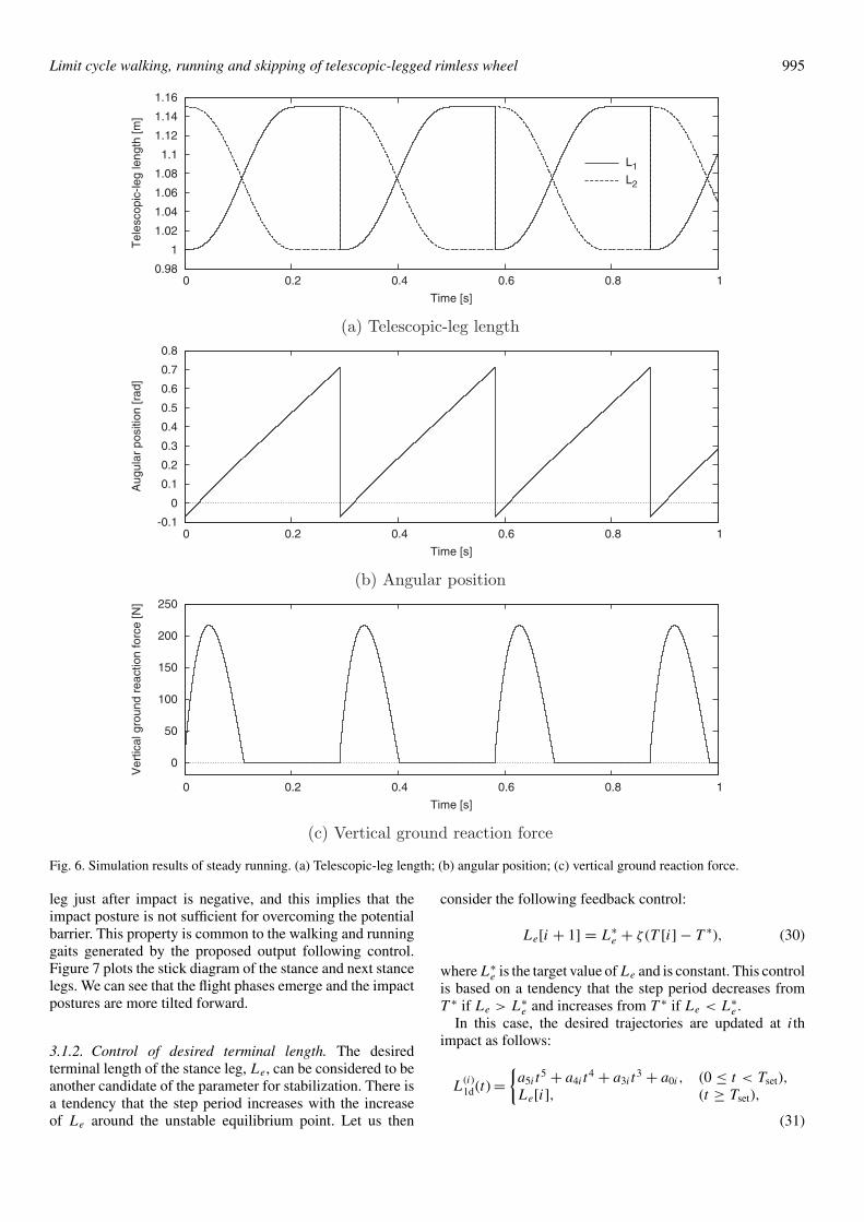
Figure 6 shows the simulation results of the steady runninggait following the above simulation. Here, (a) is the lengths ofthe telescopic legs, (b) the angular position of the stance leg,and (c) the vertical reaction force. We can see that L1 (L2)is successfully controlled from Ls (Le) to Le (Ls) during thestance and flight phases. The angular position of the stance


0.98

1

1.02

1.04

1.06

1.08

1.1

1.12

1.14

1.16

0 0.2 0.4 0.6 0.8 1

Tel

esco

pic-

leg

leng

th [m

]

Time [s]

L1

L2


-0.1

0

0.1

0.2

0.3

0.4

0.5

0.6

0.7

0.8

0 0.2 0.4 0.6 0.8 1

Aug

ular

pos

ition

[rad

]

Time [s]


0

50

100

150

200

250

0 0.2 0.4 0.6 0.8 1

Ver

tical

gro

und

reac

tion

forc

e [N

]

Time [s]


Fig. 6. Simulation results of steady running. (a) Telescopic-leg length; (b) angular position; (c) vertical ground reaction force.

leg just after impact is negative, and this implies that theimpact posture is not sufficient for overcoming the potentialbarrier. This property is common to the walking and runninggaits generated by the proposed output following control.Figure 7 plots the stick diagram of the stance and next stancelegs. We can see that the flight phases emerge and the impactpostures are more tilted forward.

3.1.2. Control of desired terminal length. The desiredterminal length of the stance leg, Le, can be considered to beanother candidate of the parameter for stabilization. There isa tendency that the step period increases with the increaseof Le around the unstable equilibrium point. Let us then

consider the following feedback control:

Le[i + 1] = L∗e + ζ (T [i] − T ∗), (30)

where L∗e is the target value of Le and is constant. This control

is based on a tendency that the step period decreases fromT ∗ if Le > L∗

e and increases from T ∗ if Le < L∗e .

In this case, the desired trajectories are updated at ithimpact as follows:

L(i)1d(t) =

{a5i t

5 + a4i t4 + a3i t

3 + a0i , (0 ≤ t < Tset),Le[i], (t ≥ Tset),

(31)


Fig. 7. Stick diagram for steady running gait.

L(i)2d(t) =

{Ls + Le[i − 1] − L

(i−1)1d (t), (0 ≤ t < Tset),

Ls, (t ≥ Tset).

(32)

Here, note that L2(0+) = Le[i − 1] and it is then smoothlycontrolled to Ls . The coefficients for the 5-order time-dependent function: a5, a4, a3, and a0, are accordinglyupdated at every instant of the stance-leg exchange asfollows:

a5i = 6(Le[i] − Ls)

T 5set

, a4i = −15(Le[i] − Ls)

T 4set

,

a3i = 10(Le[i] − Ls)

T 3set

, a0i = Ls.

Figure 8 plots the evolutions of (a) the desired terminallength, (b) the step period, and (c) the running speed withrespect to the step number. Again, the basic parameters werechosen as listed in Table I except Le. The parameters foradjustment of Le were chosen as ζ = 0.35, Tset = 0.20 s,T ∗ = 0.340 s, and L∗

e = 1.15 s. The initial value of Le wasalso chosen as Le[0] = 1.15 s. We can see that the generatedgait converges to a stable 1-period limit cycle while updatingLe.

This approach has also been shown to be effective. In thefollowing, however, we’d like to use the feedback controlof Tset only for stabilization to systematically evaluate theproperties of the walking, running, and skipping gaits underthe same rolling radius.

3.2. Efficiency analysis3.2.1. Walking speed and specific resistance. We analyzethe efficiency of the generated running gait by changing thetarget step period, T ∗. In this case, the desired settling time,Tset, cannot be systematically changed. Figure 9 plots themoving speed as a function of Tset. Since the leg mass issufficiently small compared to the hip mass, the movingspeed was approximately calculated by dividing the traveldistance of the central position of the body frame, i.e., theposition of mH , by the step period. We can see that the speedof the generated gaits is very fast and almost monotonicallyincreases with the increase of Tset. As seen from the enlargedview, however, the moving speed is not uniquely determined

with respect to Tset. This suggests that two different gaits canbe generated in accordance with the system parameters.

The energy efficiency of limit-cycle runners can beevaluated in terms of specific resistance (SR) which is definedas

SR := p

Mgv, (33)

where M := mH + 8m [kg] is the robot’s total mass and p

[J/s] is the average input power which is defined as

p := 1

T

∫ Tset

0+(|L1u1| + |L2u2|) dt. (34)

Here, SR expresses the consumed energy per unit mass andper unit length traveled, and is a dimensionless quantity. Thesmaller its value, the better the energy efficiency. Note thatthe real robot consumes energy not only by actuating thetelescopic legs but also by maintaining the lengths of theother six legs during motion. We assumed that the other sixlegs are mechanically locked and they do not need any energysupply.

Figure 10 plots the moving speed versus the SR. We can seethat there are one-to-one relationships between the movingspeed and specific resistance. It should be noted that thefaster the moving speed, the better the energy efficiency.This implies that the change in the consumed energy is muchflatter than that in the moving speed.

3.2.2. Walking versus running. Here, we compare theproperties of the generated running gait with those of thewalking gait. Figure 11 plots the moving speeds asthe functions of Tset. We also generated the walking gaitsby using the same model and parameters by changing Tset.The result strongly supports that the running gaits achievemuch faster than the walking gaits. The moving speed in therunning gait is very sensitive to Tset, whereas there is littlechange in the walking gait although the range of Tset is wide.

Figure 12 shows the comparison of the SR. In virtualgravity approaches, the minimum SR yields tan φ [-], whereφ rad is the virtual slope. As one of the authors showedin ref. [12], a compass-like biped robot with semicircularfeet achieves highly efficient limit-cycle walking with anSR of 0.01 [-] where φ = 0.01 rad. Compared with this, wemust conclude that the generated walking gaits are highly


1.142

1.144

1.146

1.148

1.15

1.152

1.154

1.156

0 5 10 15 20 25 30

Des

ired

term

inal

leng

th [m

]

Step number

(a) Desired terminal length

0.27 0.28 0.29 0.3

0.31 0.32 0.33 0.34 0.35 0.36

0 5 10 15 20 25 30

Ste

p pe

riod

[s]

Step number

With control

Without control

(b) Step period

2.6

2.7

2.8

2.9

3

3.1

3.2

0 5 10 15 20 25 30

Mov

ing

spee

d [m

/s]

Step number

With control

Without control

(c) Moving speed

Fig. 8. Convergence of gait descriptors. (a) Desired terminal length; (b) step period; (c) moving speed.

inefficient. In addition, the SR in the running gait is verysensitive to Tset, whereas there is little change in the walkinggait. It should be noted that the energy efficiency in therunning gait can be improved much better than that in thewalking gait by suitably choosing Tset.

Note that there is a gap between the running domainand the walking one. There is a potentiality, however, thatdifferent gaits would emerge in the blank area by modifyingthe condition for detection of collision in the numericalsimulator. Let us investigate this in the next section.

4. Skipping Gait Generation

4.1. AssumptionsThis section investigates the potentiality and properties oflimit-cycle skipping by using the same robot model andcontrol law.

Skipping gaits involve another collision of the stance legwith the ground at the middle of the stance phase, whichis then divided into the following five phases, as shown inFig. 13.

(1) Stance phase IThe robot equations of motion during this phase are thesame as those of the walking gait: Eqs. (2) and (4).

(2) Flight phaseAs described in Section 2.1.2, the robot begins to flightwhen the vertical ground reaction force achieves zerofrom positive. The robot equation of motion during thisphase is the same as Eq. (2), where λ = 02×1.

(3) Collision phase IThe first collision of the stance leg with the groundoccurs when z = 0. The conditions for the velocityconstraint at this phase are given by x+ = 0 and z+ = 0.We should note, however, that the stance leg will beginto shrink due to the impact force if this collision occurs


2.3

2.4

2.5

2.6

2.7

2.8

2.9

3

3.1

3.2

0.18 0.185 0.19 0.195 0.2 0.205 0.21 0.215

Mov

ing

spee

d [m

/s]

Tset [s]

3.02

3.04

3.06

3.08

3.1

3.12

3.14

3.16

3.18

0.2146 0.2147 0.2148 0.2149 0.215 3.02

3.04

3.06

3.08

3.1

3.12

3.14

3.16

3.18

0.2146 0.2147 0.2148 0.2149 0.215

Fig. 9. Moving speed as a function of Tset.

in the middle of the output following control. We thenderive the inelastic collision models depending on thesettling-time condition.The inelastic collision in this case is modeled as

M(qs)q+s = M(qs)q

−s − JT

s λs, (35)

where J s is the Jacobian matrix derived depending onthe settling-time condition. The size of J s is not unique.Let Ts [s] be the time of this collision. We assume thatthe telescopic legs are mechanically locked in the caseof Ts ≥ Tset, i.e., the settling-time condition is met. The

conditions of L+1 = 0 and L+

2 = 0 are then added, andJ s in Eq. (35) becomes

J s =

⎡⎢⎣

1 0 0 0 00 1 0 0 00 0 0 1 00 0 0 0 1

⎤⎥⎦ , (36)

which should satisfy

J s q+s = 04×1. (37)

0.11

0.12

0.13

0.14

0.15

0.16

0.17

0.18

0.19

2.3 2.4 2.5 2.6 2.7 2.8 2.9 3 3.1 3.2

Spe

cific

res

ista

nce

[-]

Moving speed [s]

Fig. 10. Moving speed versus specific resistance.


1.4

1.6

1.8

2

2.2

2.4

2.6

2.8

3

3.2

0.15 0.2 0.25 0.3 0.35 0.4 0.45 0.5 0.55 0.6

Mov

ing

spee

d [m

/s]

Tset [s]

Walking

Running

Fig. 11. Comparison of moving speeds as functions of Tset.

0.11

0.12

0.13

0.14

0.15

0.16

0.17

0.18

0.19

0.15 0.2 0.25 0.3 0.35 0.4 0.45 0.5 0.55 0.6

Spe

cific

res

ista

nce

[-]

Tset [s]

Walking

Running

Fig. 12. Comparison of specific resistances as functions of Tset.

Fig. 13. Phase sequence in skipping gait.


0.98

1

1.02

1.04

1.06

1.08

1.1

1.12

1.14

1.16

0 0.5 1 1.5 2

Tel

esco

pic-

leg

leng

th [m

]

Time [s]

L1

L2


-0.3

-0.2

-0.1

0

0.1

0.2

0.3

0.4

0.5

0.6

0 0.5 1 1.5 2

Aug

ular

pos

ition

[rad

]

Time [s]


0

50

100

150

200

250

0 0.5 1 1.5 2

Ver

tical

gro

und

reac

tion

forc

e [N

]

Time [s]


Fig. 14. Simulation results of skipping. (a) Telescopic-leg length; (b) angular position; (c) vertical ground reaction force.

Fig. 15. Stick diagram for steady skipping gait.


0.98

1

1.02

1.04

1.06

1.08

1.1

1.12

1.14

1.16

0 0.5 1 1.5 2

Tel

esco

pic-

leg

leng

th [m

]

Time [s]

L1

L2


1.1494

1.1496

1.1498

1.15

1.1502

0 0.5 1 1.5 2

Tel

esco

pic-

leg

leng

th [m

]

Time [s]

(b) Magnified view of (a)

0

50

100

150

200

0 0.5 1 1.5 2

Ver

tical

gro

und

reac

tion

forc

e [N

]

Time [s]


Fig. 16. Simulation results of skipping. (a) Telescopic-leg length; (b) magnified view of (a); (c) vertical ground reaction force.

Whereas in the case of Ts < Tset, we assume that thetelescopic legs keep driving and are not mechanicallylocked. J s in Eq. (35) then becomes

J s =[

1 0 0 0 00 1 0 0 0

], (38)

which should satisfy

J s q+s = 02×1. (39)

By the effect of the output following control, however,the lengths of the telescopic legs are controlled to Le

and Ls again for a short time.

(4) Stance phase IIAll equations are the same as those of stance phase I.

(5) Collision phase II (Stance-leg exchange)The second collision occurs when the next stance leghits the ground. All equations for the inelastic collisionmodel are the same as those of the walking gait inSection 2.1.3: Eqs. (6) and (7).

4.2. Typical gaitWe first try to generate a stable skipping gait. Unlike running,a skipping gait emerges only by conducting the outputfollowing control with a suitable settling of Tset. Figure 14shows the simulation results of the steady skipping gaitwhere Tset = 0.25 s. Here, (a) represents the lengths of the


1.2

1.4

1.6

1.8

2

2.2

2.4

2.6

2.8

3

0.1 0.15 0.2 0.25 0.3 0.35 0.4 0.45 0.5

Mov

ing

spee

d [m

/s]

Tset [s]

Walking

Running

Skipping (locked)

Skipping (unlocked)

1.41

1.42

1.43

1.44

1.45

1.46

1.47

1.48

0.24 0.26 0.28 0.3 0.32 0.34 0.36 0.38

Fig. 17. Moving speeds as function of Tset.

telescopic-legs, (b) the angular position, and (c) the verticalground reaction force. Figure 15 shows the stick diagramfor the three steady steps. Again, the physical parameterswere chosen as the same as those in the previous sections. Inthis case, the first collision of the stance leg with the ground(collision phase I) occurs more than 0.20 s after the stance-leg exchange (collision phase II). Therefore, the telescopiclegs are mechanically locked and the robot lands on theground as a 1-DOF rigid body. We can see that a skippinggait is successfully generated in accordance with the phasesequence of Fig. 13.

Figure 16 shows the simulation results of the steadyskipping gait where Tset = 0.31 s. Here, (a) represents thelengths of the telescopic legs, (b) the magnified view of L1

in (a), and (c) the vertical ground reaction force. In this case,the first collision of the stance leg occurs in the middle ofthe output following control, i.e. Ts < Tset, and the telescopiclegs are thus unlocked at the instant. From (b), we can seethat the stance leg immediately begins to start shrinking justafter impact but it returns to Le = 1.15 m before the nextimpact. Although we omit the details, the previous stance legalso a bit overshoots the nominal length, Ls = 1.0 m, due tothe effect of the impact force but it returns to Ls soon. (c)also shows that the time change of vertical ground reactionforce is similar to that of Fig. 14 (c) but it is affected by thecontrol force of the stance leg, u1, for pushing back just afterthe first collision.

4.3. Efficiency analysisWe evaluate the gait efficiency in terms of the walking speedand SR. Figure 17 plots the moving speeds of the three dif-ferent gaits as functions of Tset. We can see that the skippinggaits emerge as an extension of the walking gaits, and that themoving speed monotonically decreases with the decrease ofTset. In addition, the skipping gaits unlocked at the collisionphase I emerge near the boundary with the walking gait.

Figure 18 plots the SR of the three different gaits asfunctions of Tset. We can see that the SR in the walkingand skipping gaits monotonically increases with the decreaseof Tset and worsens more rapidly after the gait transition.From the magnified view, we can also see that the increasingtendency of the SR with respect to the decrease of Tset in theunlocked case is more rapid than that in the locked case. Thisis caused by the additional control force needed for extendingthe stance leg after shrinking due to the first collision.

We must conclude that the efficiency of the skipping gaitsis the worst. Homogeneity of the walking and skipping gaits,however, creates an understanding that the stable domain oflimit-cycle walking is dramatically extended by consideringthe condition of limit-cycle skipping.

Note that the range of Tset (stable domain) of the skippinggait overlaps with that of the running gait. Note also that, aspreviously described, the stable running gaits could not begenerated without the feedback control of Tset. These implythat the running gait is different in properties from the othertwo gaits. Two factors make the difference. One is the initialangular velocity. A skipping gait can also be generated withthe feedback control of Tset if the robot starts from a slowerangular velocity. If we set the initial angular velocity to asufficiently fast one, the gait converges to a stable runninggait of the same Tset. The other is the inherent stability.Limit cycle gaits that are inherently stable naturally emergeunder the suitable parameter settings, whereas those that areinherently unstable need specialized control techniques forstabilization. If the three different gaits can be dealt withfrom a unified standpoint, the design of a controller foradaptation to diverse situations would be formulated. Moreinvestigations are necessary.

5. Conclusion and Future WorkIn this paper, we investigated the properties of the walking,running, and skipping gaits of the telescopic-legged rimless


0.1

0.15

0.2

0.25

0.3

0.35

0.4

0.1 0.15 0.2 0.25 0.3 0.35 0.4 0.45 0.5

Spe

cific

res

ista

nce

[-]

Tset [s]

Walking

Running

Skipping (locked)

Skipping (unlocked)

0.145

0.15

0.155

0.16

0.165

0.17

0.175

0.18

0.24 0.26 0.28 0.3 0.32 0.34 0.36 0.38

Fig. 18. Specific resistances as function of Tset.

wheel. It was shown that the proposed method based onrobot’s forward-tilting impact posture can also be used forgenerating the other two gaits only by adjustment of thedesired settling time. Through the detailed gait analysis,we have learned two important features. One is that thegenerated walking and skipping gaits are inherently stablebut the running gait is unstable only with the output followingcontrol. The other is that, by considering skipping, the stabledomain of the walking gait is dramatically extended but thegait efficiency grows worse in terms of the moving speed andSR.

It would be expected that more various and adaptive gaitsare generated by applying a unified controller taking thethree gaits’ properties into account. For this achievement, itis necessary to deeply understand the difference in stabilitybetween the running gait and the other two gaits. Improveddesign of limit-cycle runners is also left as an importantsubject to be investigated. There is a probability of makingthe running gait inherently stable and more energy-efficientby appropriately modifying the robot’s body shape andmechanisms. Incorporating springs is a solution candidatefor improving the energy-efficiency. Equivalent control lawsusing passive compliance mechanisms and the effect on thegait properties should also be investigated in the future.

References1. T. McGeer, “Passive dynamic walking,” Int. J. Robot. Res. 9(2),

62–82 (Apr. 1990).2. R. M. Alexander, Principles of Animal Locomotion (Princeton

University Press, Princeton, NJ, USA, 2003).

3. T. McGeer, “Passive bipedal running,” Proc. R. Soc. Lond. Ser.B, Biol. Sci. 240(1297), 107–134 (May 1990).

4. M. Ahmadi and M. Buehler, “Stable control of a simulatedone-legged running robot with hip and leg compliance,” IEEETrans. Robot. Autom. 13(1), 96–104 (Feb. 1997).

5. F. Iida, J. Rummel and A. Seyfarth, “Bipedal Walking andRunning with Compliant Legs,” Proceedings of the IEEEInternational Conference on Robotics and Automation (Apr.2007) pp. 3970–3975.

6. F. Asano, “Dynamic Gait Generation of Telescopic-LeggedRimless Wheel Based on Asymmetric Impact Posture,”Proceedings of the 9th IEEE-RAS International Conferenceon Humanoid Robots, Paris, France (Dec. 2009) pp. 68–73.

7. F. Asano and M. Suguro, “High-Speed Dynamic GaitGeneration Based on Forward Tilting Impact Posture UsingTelescopic Legs and Forefeet,” Proceedings of the 13thInternational Conference on Climbing and Walking Robotsand the Support Technologies for Mobile Machines (CLAWAR2010), Nagoya, Japan (Sep. 2010) pp. 729–736.

8. F. Asano, “High-Speed Biped Gait Generation Based onAsymmetrization of Impact Posture Using Telescopic Legs,”Proceedings of the IEEE/RSJ International Conference onIntelligent Robots and Systems, Taipei, Taiwan (Oct. 2010)pp. 4477–4482.

9. S. Collins, A. Ruina, R. Tedrake and M. Wisse, “Efficientbipedal robots based on passive-dynamic walkers,” Science307(5712), 1082–1085 (Feb. 2005).

10. C. T. Farley, “Locomotion: Just skip it,” Nature 394, 721–723(Aug. 1998).

11. A. E. Minetti, “The biomechanics of skipping gaits: A thirdlocomotion paradigm?,” Proc. R. Soc. Lond. Ser. B, Biol. Sci.,265(1402), 1227–1235 (Jul. 1998).

12. F. Asano and Z.-W. Luo, “On Energy-Efficient and High-Speed Dynamic Biped Locomotion with Semicircular Feet,”Proceedings of the IEEE/RSJ International Conference onIntelligent Robots and Systems, Beijing, China (Oct. 2006)pp. 5901–5906.

limit cycle walking, running, and skipping of the effect of high-speed telescopic-legs’ actuation....

Documents