s

over 500potsshape, butenly, grow

during the6.8 daysntirerger thanrees withjets have

t violate theardthe Greatprobable

ing spots,RS over its

Icarus 172 (2004) 9–23www.elsevier.com/locate/icaru

Life cycles of spots on Jupiter from Cassini images

Liming Li a,∗, Andrew P. Ingersolla, Ashwin R. Vasavadab, Carolyn C. Porcoc,Anthony D. Del Geniod, Shawn P. Ewalde

a Division of Geological and Planetary Sciences, MS 150-21, California Institute of Technology, Pasadena, CA 91125, USAb Department of Earth and Space Sciences, University of California Los Angeles, Los Angeles, CA 90095, USA

c Southwest Research Institute, Boulder, CO 80302, USAd NASA Goddard Institute for Space Studies, Broadway, New York, NY 10025, USA

e Division of Geological and Planetary Sciences, California Institute of Technology, Pasadena, CA 91125, USA

Received 12 February 2003; revised 24 September 2003

Available online 20 December 2003

Abstract

Using the sequence of 70-day continuum-band (751 nm) images from the Cassini Imaging Science System (ISS), we recordcompact oval spots and study their relation to the large-scale motions. The∼ 100 spots whose vorticity could be measured—the large sin most cases—were all anticyclonic. We exclude cyclonic features (chaotic regions) because they do not have a compact ovalwe do record their interactions with spots. We distinguish probable convective storms from other spots because they appear suddrapidly, and are much brighter than their surroundings. The distribution of lifetimes for spots that appeared and disappeared70-day period follows a decaying exponential with time constant (mean lifetime) of 3.5 days for probable convective storms and 1for all other spots. Extrapolating the exponential beyond 70 days seriously underestimates the number of spots that existed for the e70-day period. This and other evidences (size, shape, distribution in latitude) suggest that these long-lived spots with lifetime la70 days are from a separate population. The zonal wind profile obtained manually by tracking individual features (this study) agthat obtained automatically by correlating brightness variations in narrow latitude bands (Porco et al., 2003). Some westwarddeveloped more curvature and some have developed less curvature since Voyager times, but the number of westward jets thabarotropic stability criterion is about the same.In the northern hemisphere the number of spots is greatest at the latitudes of the westwjets, which are the most unstable regions according to the barotropic stability criterion. During the 70-day observation periodRed Spot (GRS) absorbed nine westward-moving spots that originated in the South Equatorial Belt (SEB), where most of theconvective storms originate. Although the probable convective storms do not directly transform themselves into westward-movtheir common origin in the SEB suggests that moist convection and the westward jet compose a system that has maintained the Glong lifetime. 2003 Elsevier Inc. All rights reserved.

Keywords: Atmospheres, dynamics; Jupiter, atmosphere; Meteorology

al-ave

gs.izeor

ure9;

,

re-the

intsrbedandcessith

1. Introduction

Jupiter’s atmosphere is full of spots—compact, ovshaped cloud features whose appearance, at some wlengths at least, is different from that of their surroundinThis contrast may reflect differences in composition or sof the cloud particles, differences in optical thicknessaltitude of the cloud, or differences in small-scale textof the cloud (Smith et al., 1979; Ingersoll et al., 197

* Corresponding author.E-mail address: liming@gps.caltech.edu (L. Li).

0019-1035/$ – see front matter 2003 Elsevier Inc. All rights reserved.doi:10.1016/j.icarus.2003.10.015

-

Mitchell et al., 1979). Some spots have lightning in themas revealed in night side images(Little et al., 1999; Gieraschet al., 2000).

Spots form in a variety of ways(Mac Low and Ingersoll,1986). Some gather contrast slowly in an otherwise featuless region; some develop coherence and emerge fromturbulent flow; and others appear suddenly as bright poand grow by expansion. Likewise, some spots are absoby the turbulent flow; some are destroyed by mergers;others simply fade away. “Life cycles” refers to appearanand disappearances, mutual interactions, and interactionwith the zonal jets. Comparing the observed life cycles w

10 L. Li et al. / Icarus 172 (2004) 9–23

;ng

1 toingters

,ingthe

-

i.e.,timeedo20 htsling

with

ageion.ALges

legle,Thelin-

sionnm

-day

selfennsis-ver

ererarets a

the

–

ing

ot’s

Weestm apotsre,therightholesorbs

and

y-engen-

nst to

tchinctex-

cultR is

-rm

ysribelike

and

sar-

t thevor-size.ally

mi-hole

pear-nce

y-s in a

and

those produced in numerical models (e.g.,Ingersoll andCuong, 1981; Williams and Yamagata,1984; Marcus, 1988Dowling and Ingersoll, 1989) leads to a better understandiof the dynamics of Jupiter’s atmosphere.

Our study uses data spanning 70 days (OctoberDecember 9, 2000) of observation by the Cassini ImagScience System (ISS) in a filter centered at 751 nanomeThe only other comparable study(Mac Low and Ingersoll1986)used 58 days of observation by the Voyager imagsystem in the violet filter. In both cases the resolution ofraw images ranged from∼ 500 km/pixel at the beginningof the sequence to∼ 100 km/pixel at the end. Voyager imaged the disk of the planet every 1/5 of a jovian rotationand covered the entire planet once per jovian rotation,once every 10 h. The mosaics became a movie withstep∼ 10 h and duration∼ 58 Earth days. Cassini operatin much the same way, except it often skipped a rotation sthat the time step was sometimes 10 h and sometimesMorales-Juberias et al. (2002), hereinafter MJ, studied spousing HST data over a 6-year period. The temporal sampis less dense than ours, but we will compare our resultstheirs wherever possible.

Each Cassini image was navigated by fitting (in the implane) the observed planetary limb to its predicted locatRadiometric calibration was performed using the CISSCsoftware developed by the Cassini ISS Team. The imafor each rotation were projected into a simple cylindricamap spanning 360 of longitude. Illumination effects werremoved by dividing by the cosine of the incidence anand regions shared by multiple images were averaged.final maps were converted to 8-bit images using the sameear stretch for all maps and are stored without compresTo date, these steps have been performed for the 751filter only, although raw images spanning the same 70period exist for several other filters.

Each Cassini mosaic is 3600× 1801 pixels and span360 of longitude and 180 of latitude. Therefore each pixspans 0.1 of longitude and 0.1 of latitude. The scale o0.1/pixel, or ∼ 125 km/pixel at the equator, was chossuch that all the 70-day images could be mapped cotently without loss of information. The spatial areas owhich spots are measured include all 360 in longitude and80 S to 80 N in latitude. The gases in Jupiter’s troposphare transparent in the 751-nm band, so these near-infcontinuum band images can capture a multitude of spodifferent altitudes in the troposphere of Jupiter.

We use the term “spot” to describe a structure havingfollowing four characteristics:

(1) compact oval shape,(2) appearance in at least three successive images (life

history at least 40 h),(3) a marked brightness difference from the surround

clouds,(4) diameter at least 700 km during some part of the sp

life.

.

.

.

dt

According to this definition, we record over 500 spots.observe the sign of the vorticity for about 100 of the largspots, whose rotation direction can be determined fromovie made from these images, and find that all these sare anticyclonic (clockwise in the northern hemisphecounterclockwise in the southern hemisphere). Among517 compact spots we record, 306 compact spots are band 211 compact spots are dark. The dark spots may bein the clouds or they may be dark cloud material that absthe light at 751 nm. Other studies(Banfield et al., 1998)sug-gest that bright and dark contrast originates at∼ 0.7 bar. Weuse planetographic latitudes, system III west longitudes,positive zonal winds in the eastward direction.Mac Lowand Ingersoll (1986)recorded over 100 spots in the Voager mosaics. Their study focused on interactions betwespots. Our study is larger (500 vs 100 spots) and moreeral; it includes appearances, disappearances, distribution oflifetimes, size distribution, mutual interactions, interactiowith the Great Red Spot (GRS), distribution with respeclatitude, and motion relative to the zonal jets.

We use the term chaotic region (CR) to define a paof rapidly changing, amorphous features. CR’s are distfrom compact spots, and are not included in our studycept as they interact with spots. In many cases it is diffito define the boundaries of a CR, and in some cases a Csimply a cyclonic band circling the entire planet.Smith et al.(1979) called these patches “disturbed regions.”Ingersollet al. (1979) and Mitchell et al. (1979)used the term “turbulent, folded-filament regions.” They also used the te“oblong cyclones,” since the vorticity of the CR’s is alwacyclonic. These authors used the term “wakelike” to descthe CR’s to the west of the large ovals. The largest wakeregion is the South Equatorial Belt (SEB) to the westslightly equatorward of the Great Red Spot (GRS).Youssefand Marcus (2003)point out that a row of cyclonic CR’alternating with a row of anticyclonic ovals resembles a Kman vortex street. With a numerical model they show tharelative positions of the vortices are stable. In a classictex street the cyclones and anticyclones have the sameOn Jupiter the east–west dimension of the CR’s is usugreater than that of the associated ovals.

2. Appearances and disappearances

Figure 1 shows that the number of appearancesnus disappearances oscillates around zero. Over the wperiod the numbers of appearances (393) and disapances (356) are basically in balance, and their differe(393− 356= 37) is not statistically significant. The null hpothesis is that both appearances and disappearance70-day period have a mean of 374.5 = (393+ 356)/2. Thestandard deviation of each is 374.51/2 = 19.4. The standarddeviation of their difference is(2 × 374.5)1/2 = 27.4. Theactual difference is 37, which is 1.35 standard deviationsnot statistically significant.

Life cycles of spots on Jupiter 11

minus

Fig. 1. The numbers of appearances and disappearances of spots every 60 hduring the 70-day period. The figure also shows the value of appearancedisappearance during the period.

s,ncesour

deateddedof

r ofitaryrancear-did

theba

e-

tur-

pid

es 2in-besave0;

ata.

ec-00

on-

blyr fil-nds.erethe

aindses).

s wed wetself.e inp-

tec-(31

Mac Low and Ingersoll (1986)observed 23 merger23 other kinds of disappearances, and 19 appeararoughly an order of magnitude fewer events than instudy. These authors noted that the number of spotsstroyed was a factor of 2 greater than the number creduring the 58-day observation period, and recommenfurther study of the budget. However, the main goaltheir paper was to study the time-dependent behaviointeracting spots. The appearance of a spot is a solevent. The fact that they observed less than one appeaper day whereas we observed more than four appances per day suggests that Mac Low and Ingersollnot record most of those events. In the long run,appearance and disappearance of spots should be inance.

We divide appearances into three types:

(1) development of contrast inan otherwise featureless rgion,

(2) development of a coherent structure in an otherwisebulent region,

(3) sudden appearance of a bright point followed by raexpansion in size.

Type 1 usually takes place outside the CR’s, whereas typand 3 usually take place in the CR’s. Type 2 oftenvolves ejection of the spot from a CR. Type 3 descrithe rapidly growing, easily identified features that often hlightning in them(Little et al., 1999; Gierasch et al., 200Ingersoll et al., 2000). Porco et al. (2003)referred to theseas “convective storms” in their analysis of the Cassini d

,

-

e

l-

However, neitherPorco et al. (2003)nor we observed thlightning directly, so we will call them “probable convetive storms.” The resolution in our images ranges from 1to 500 km, which is enough to resolve the probable cvective storms in the SEB (10 S–16 S) and the NEB(10 N–15 N). Compared withPorco et al. (2003)we didnot find many convective storms at other latitudes, probabecause we used just the 751 nm filter and they used otheters including those in the strong and weak methane baConvective storms are important for the jovian atmosphbecause they can transport much of the heat flux fromdeeper troposphere(Gierasch et al., 2000).

Figure 2adisplays an example of a spot developing inrelatively calm area (type 1). This is the most frequent kof appearance among the three types (221 out of 393 caThe gradual appearance of the spot inFig. 2ais not due to thechange in resolution, because in the first two subimagecan see that the embryo did not have elliptical shape ancan see much smaller scale features than the embryo iFigure 2bshows a spot that emerged from the turbulenca CR (type 2). This is the next most frequent kind of apearance (141 out of 393).Figure 3ashows a very brighspot that grows rapidly (type 3), and is probably a convtive storm. This is the least frequent kind of appearanceout of 393 cases).

We also divide disappearances into three types:

(1) disappearance due to merging,(2) destruction by the turbulence, usually in a CR,(3) gradual fading.

12 L. Li et al. / Icarus 172 (2004) 9–23

osuchis

Fig. 2. (a) Large spot developing slowly outside of a CR. In this figure and all other figures like it (Figs. 2b, 3a, 3b, 4a, and 4b), time increases from top tbottom. Note that the time step between neighboring subimages ofFig. 2ais 10 days, so the spot is developing very slowly. The time step for all otherfigures (Figs. 2b, 3a, 3b, 4a, and 4b) is 20 h. The range for every frame ofFig. 2ais (12 N–23 N, 350–17). The time of the first subimage (the top one)Oct 5, 2000. The large spot covers the center of the 17 N westward jet. (b) Spot coming from a CR. The range for every frame is (42 N–54 N, 230–267).The time of the first subimage is Nov 5, 2000. The spot sits in an anticyclonic band.

oferp-

ous,

g-

t therea

Weasseringrging

bu-s fornces

of

anyindisap-

cat-tersivedy pe-andhites.i-nt

tsived

Figure 3bshows a merger between two spots. This typedisappearance is different from destruction by turbulenc(Fig. 4a) because it results in a recognizable spot. Absotion by turbulence results in more turbulence—amorphrapidly changing patterns that have no definite spots.MacLow and Ingersoll (1986)were especially interested in merers because the solitary wave model(Maxworthy et al.,1978)predicted that when one spot overtakes another asame latitude they would pass through each other, wheother models(Ingersoll and Cuong,1981; Williams and Ya-magata, 1984)predicted that the two spots would merge.record 119 mergers and 7 near misses—where spots paround each other—out of the total 126 interactions duthe 70-day period. Our result seems to support these memodels.

Figure 4ashows a small spot that is destroyed by turlence inside a CR. This kind of disappearance accountmore than one-fourth of the total number of disappeara(90 out of 356). CR’s are not only an important sourcespots but also an important sink of spots.Figure 4bshows

s

d

a spot that fades away. It disappears without undergoinginteraction with other spots or CR’s. The number of this kof disappearance is largest among the three types of dpearance (147 out of 356 cases).

3. Dimensions

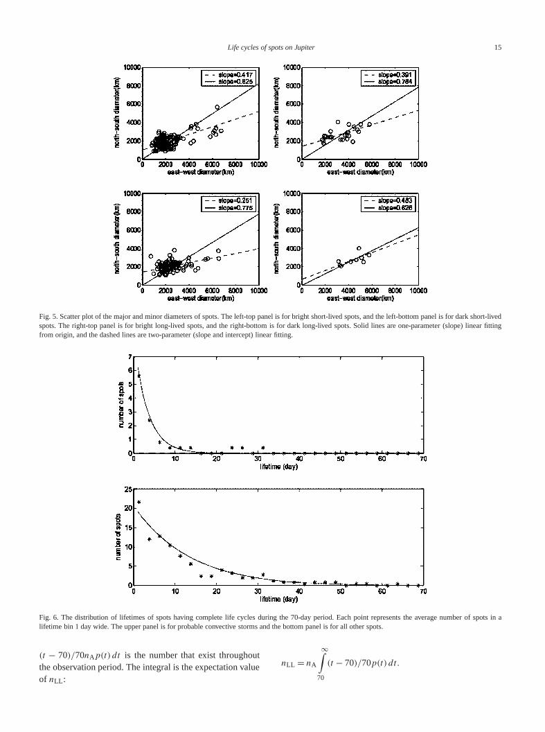
In Fig. 5we record the sizes of all spots and give a ster plot of north–south (NS) and east–west (EW) diamebased on the brightness and lifetime. In our study, long-lspots are those that existed throughout the entire 70-dariod, and short-lived spots are those that both appeareddisappeared during the 70-day period. The GRS and woval at−33 are not included in the list of long-lived spotFigure 5offers two different linear fits between the two dameters by assuming that theuncertainties of measuremein major and minor diameters are the same(Meyer, 1986).The fitting lines from the origin indicate that long-lived spoand dark spots have smaller NS/EW ratios than short-l

Life cycles of spots on Jupiter 13

s

Fig. 3. (a) A fast-developing spot in a CR, probably a convective storm. The range for every frame is (9 N–17 N, 8–30). The time of the first subimage iOct 29, 2000. The spot sits in a cyclonic band. (b) Two spots merging with each other. The range for every frame is (38 N–45 N, 280–295). The time ofthe first subimage is Nov 13, 2000. The two spots sit in an anticyclonic band.

dif-ving

di-em.

thef thewithin-ase

of,toryam

-ithusg a

s

spots and bright spots. The two-parameter fit presents aferent result because it is more sensitive to spots haextreme low and high ratios than the fit from the origin.

Figure 5shows that all the long-lived spots have majorameters greater than∼ 2000 km. The short-lived spots havmajor diameters ranging from below 1000 to over 6000 kThere is no correlation between lifetime and size forshort-lived spots, and we cannot measure the lifetimes olong-lived spots. Our results are generally in agreementFigs. 4 and 6of MJ, although our study has a smaller mimum spot size (700 vs 1500 km) and a shorter time bthan theirs.

4. Distribution of lifetimes

The time between the appearance and disappearancea spot is its lifetime.Figure 6is a histogram of lifetimesconstructed using those spots having a complete life hisduring Cassini’s 70-day observation window. The histogrhas a bias, which is correctable: A spot with lifetimet < 70days must appear in the initial (70− t ) days of the observation window to be included in the histogram. Spots wlifetimest > 70 days are not included in the histogram. Thif nA is the average number of spots that appear durin70 day window andp(t) dt is the fraction whose lifetime

14 L. Li et al. / Icarus 172 (2004) 9–23

hec

0.

Fig. 4. (a) A small spot destroyed by aCR. The range for every frame is (46 N–57 N, 90–117). The time of the first subimage is Nov 25, 2000. Tspot sits in an anticyclonic band and meets the left side of a turbulent structure in the CR. (b) A spot that lost contrast and faded away. Sometimes thisaseresembles that inFig. 4a, absorption by turbulence. The range for every frame is (42 N–48 N, 310–324). The time of the first subimage is Nov 18, 200The spot covers the center of the 45 N eastward jet.

r in

thee ex

d-

righes

owslifeof

that

n

nd

ehepot

s ifn a

are in the range(t, t + dt), then(70− t)/70nAp(t) dt is thenumber in this lifetime range that appear and disappeathe window. This is the histogram displayed inFig. 6.

In Fig. 6, the fitted curves show(70− t)/70nAp(t) dt ,where dt = 1 day andp(t) = (1/τ)exp(−t/τ ). For thevalue ofnA we average the number of appearances andnumber of disappearances, since the two are the samcept for statistical fluctuations. This givesnA = 29.5 for theupper panel andnA = 345 for the lower panel. The one ajustable parameter isτ , and the fitting yieldsτ = 3.5 daysfor the probable convective storms andτ = 16.8 days for allother spots. We separated the latter (other spots) into a bgroup and a dark group, and fit the distribution of lifetimfor the two groups separately (not shown). The fitting shthat the time constant of bright spots having a completehistory (τ = 14 days) is smaller than the time constantdark spots having a complete life history (τ = 21 days).

-

t

The expectation value for the total number of spotsappear and disappear in the window is

nAD = nA

70∫

0

(70− t)/70p(t) dt.

The expected numbernAO of spots that only appear ithe window and disappear later isnA − nAD. The expectednumbernDO of spots that only disappear in the window aappear earlier is alsonA − nAD. Actual numbers will be dif-ferent because of statistical fluctuations.

Information about lifetimet > 70 days is contained in thnumbernLL of long-lived spots that existed throughout tobservation period. To be included in this number, a swith lifetime t must appear no more than(t − 70) days be-fore the start of the Cassini observation window. ThunAp(t) dt is the average number of spots appearing i70 day window with lifetimes in the range(t, t + dt), then

Life cycles of spots on Jupiter 15

ts

Fig. 5. Scatter plot of the major and minor diameters of spots. The left-top panel is for bright short-lived spots, and the left-bottom panel is for darkshort-livedspots. The right-top panel is for bright long-lived spots, and the right-bottom is for dark long-lived spots. Solid lines are one-parameter (slope) linear fittingfrom origin, and the dashed lines are two-parameter (slope and intercept) linear fitting.

Fig. 6. The distribution of lifetimes of spots having complete life cycles during the 70-day period. Each point represents the average number of spoin alifetime bin 1 day wide. The upper panel is for probable convective storms and the bottom panel is for all other spots.

utalue

(t − 70)/70nAp(t) dt is the number that exist throughothe observation period. The integral is the expectation vof nLL :

nLL = nA

∞∫

70

(t − 70)/70p(t) dt.

16 L. Li et al. / Icarus 172 (2004) 9–23

2728

339

luessfit to

ee-

istebertire. Evtheome

areedandassin

neST98;

-oudmi-

t theare

forol-es,eedcanotionctionratocor-60wesbe-rrors

, andion

od istruc-

60 hthis

esslue

heinsta-city

iffer-

ts.at

ment

odhe

toro-

dataan

s.

ardilityoreata

n-

r,r

dite-calain

-jets

Table 1Number of appearances and disappearances

nLL nAO nDO nAD

Probable convective storms (expected) 0 2 2Probable convective storms (observed) 0 3 0

All other compact spots (expected) 1 82 82 26All other compact spots (observed) 35 123 89 2

nLL = long-lived spots, lifetime> 70-days.nAO = appear only, disappear later.nDO = disappear only, appeared earlier.nAD = appear and disappear in the 70-day period.

In Table 1we compare the observed and expected vaof nLL , nAO, nDO, andnAD for probable convective stormand for all other spots. The expected values use the bestthe histogram inFig. 6, with τ = 3.5 days for the probablconvective storms andτ = 16.8 days for all other spots. Thnumber of appearances isnAO +nAD, and the number of disappearances isnDO + nAD. Except fornLL , the differencesbetween the observed and expected numbers are conswith statistical fluctuations. However, the expected numof nonconvective (other) spots that survive for the en70-day period is 1, whereas the observed number is 35idently there are more spots with long lifetimes thanexponential distribution would suggest. There is even sevidence that the spots with lifetimes longer than 70 daysfrom a different population: As shown below, the long-livspots have different distributions with respect to latitudesize than the spots that appear and disappear in the Cobservation window.

5. Relation to zonal winds

Much work on zonal winds of Jupiter has been dobased on the data sets of Voyager, Galileo, and H(Ingersoll et al., 1981; Limaye, 1986; Vasavada et al., 19Garcia-Melendo and Sanchez-Lavega, 2001). These studies support the idea that the zonal wind profile at the cllevel has remained basically unaltered in spite of somenor variations in jet shape and speed. This implies thaglobal circulation of Jupiter is stable even though thereturbulence and convection in the atmosphere.

Feature tracking and correlation are two methodsmeasuring the wind velocity on Jupiter. By manually flowing the target clouds in images taken at different timthe feature tracking method can determine the wind spat the latitudes where these target clouds sit, if cloudsbe regarded as passive tracers of atmospheric mass mFor this method, the change of feature shape, the interabetween these clouds and their environment, and opejudgment will cause some errors. On the other hand, therelation method takes a narrow latitude band spanning 3in longitude as the target and determines its mean east–movement by finding the largest correlation coefficienttween two images taken at different times. Systematic e

nt

-

i

.

r

t

caused by changes of the clouds, wave-like phenomenalarge vortices (GRS, for example) will affect the correlatmethod(Garcia-Melendo and Sanchez-Lavega, 2001). Bothmethods are sensitive to spots, but the correlation methalso sensitive to amorphous features and large-scale stures that a human operator might ignore.

In our study, we record the position of each spot everyand compute a velocity based on its displacement over60 h time interval. If the spot changes latitude by lthan 1, and if it changes velocity from the average vafor its complete life history by less than 10 m s−1, then wewill use the spot as a record for the wind velocity of tlatitude in which it sits. In addition, for these latitudeswhich there are few spots we use other features havingble nonoval shape as tracking targets to get the wind velofor these latitudes. Then we average these records in dent 1 bins to get the wind velocity for latitudes from 78 Sto 83 N. This was impossible for some latitudes (77 N,25 N, 21 N, 16 N, 10 N, 2 N–5 N, 1 S, 14 S, 26 S,30 S, 37 S, 44 S, 54 S, 61 S, 63 S, 67 S–70 Sand 77 S) where we could not find good tracking targeWe use interpolation to get the values of wind velocitythese latitudes.

Figure 7 shows that the wind profile obtained froCassini by the feature tracking method is in good agreemwith the wind profile obtained by the correlation meth(Porco et al., 2003). The correlation coefficient between ttwo profiles from 78 S to 83 N is 0.9257.Porco et al.(2003)study changes in the jets from the Voyager timethe Cassini time. Further study of the changes of wind pfiles requires a detailed discussion of the accuracy offrom different sources (Voyager, HST and Cassini) anderror analysis of velocity measurement in all these studieSuch an effort is beyond the scope of this study.

Using the data of Voyager, Ingersoll et al. (1979, 1981)andLimaye (1986)discussed the curvature of the westwjets and the jets’ stability according to the barotropic stabcriterion. In this paper, we repeat this work based on mdata including Voyager, HST and Cassini. The Voyager d(Limaye, 1986)were taken in 1979. The HST data(Garcia-Melendo and Sanchez-Lavega, 2001)were taken from 1995to 2000. The Cassini data were taken in 2000.

The barotropic stability criterion says that a two-dimesional (barotropic) flow is stable whenβ − uyy > 0 at alllatitudes. Hereβ = df/dy = 2Ω cosφ/RJ is the planetaryvorticity gradient,f = 2Ω sinφ is the Coriolis parameteφ is planetographic latitude,Ω andRJ are Jupiter’s angularate of rotation and planetary radius, respectively;u is themean zonal wind,y is the northward coordinate, anduyy isthe curvature of the jets. Sinceβ is positive everywhere anuyy is positive at the latitudes of the westward jets, the crrion is most likely to be violated at these latitudes. Vertistructure in the flow can alter its stability, but it is uncertand we do not discuss it here.

Figure 8shows parabolas with curvatureβ that are centered on the westward jets. The figure shows that some

Life cycles of spots on Jupiter 17

cm

000)ssinisured

Fig. 7. The zonal wind profile obtainedfrom Cassini by two different methods—feature tracking and correlation. Both wind profiles use planetographilatitudes. In the left panel, each point is a single feature, and the solid line is the average of the points in a 1 bin. In the right panel, the two lines are frofeature tracking in this study and correlation method fromPorco et al. (2003).

Fig. 8. Curvatured2u/dy2 of the zonal velocity profile compared toβ. From left to right the data are from Voyager (1979), HST (1995–2000), Cassini (2feature tracking, and Cassini correlation. The parabolic curves are defined byd2u/dy2 = β, and are centered on the westward jet maxima. For the Cafeature tracking profile, each point is an average of features in a 1 latitude bin. For the other profiles the resolution is 2–3 times better. Where the meaprofile lies inside the parabola, the flow violates the barotropic stability criterion.

18 L. Li et al. / Icarus 172 (2004) 9–23

ssjeter

ing

menkingrelaardisand

i-weshowistrits areyuld

mi-ot a

te-and

Whites

snicatest-seri-ablethe

-

the(seetedJeen) vse istwo

tomhe

less

eirdata

developed more curvature thanβ and others developed lecurvature thanβ during the 21 years 1979–2000. Theat 39 N had uyy > β during HST time and less at othtimes. The jet at 31 N had uyy > β during Voyager timeand less at other times. The jet at 17 N had uyy > β dur-ing Voyager times and less at other times. The jet at 20 Shaduyy > β during HST and Cassini times and less durVoyager times. The jet at 32 S haduyy > β during Voy-ager time and less at other times. The general agreebetween HST and Cassini and between the feature tracand correlation methods suggests that the differencestive toβ are significant. In general, the number of westwjets that clearly violate the barotropic stability criterionabout the same during Cassini time as during VoyagerHST times.

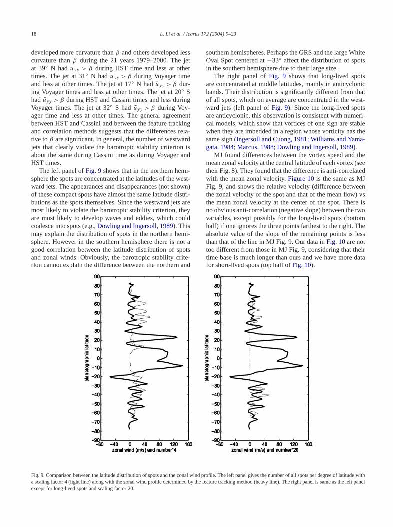
The left panel ofFig. 9 shows that in the northern hemsphere the spots are concentrated at the latitudes of theward jets. The appearances and disappearances (not sof these compact spots have almost the same latitude dbutions as the spots themselves. Since the westward jemost likely to violate the barotropic stability criterion, thare most likely to develop waves and eddies, which cocoalesce into spots (e.g.,Dowling and Ingersoll, 1989). Thismay explain the distribution of spots in the northern hesphere. However in the southern hemisphere there is ngood correlation between the latitude distribution of spotsand zonal winds. Obviously, the barotropic stability cririon cannot explain the difference between the northern

t

-

t-n)-e

southern hemispheres. Perhaps the GRS and the largeOval Spot centered at−33 affect the distribution of spotin the southern hemisphere due to their large size.

The right panel ofFig. 9 shows that long-lived spotare concentrated at middle latitudes, mainly in anticyclobands. Their distribution is significantly different from thof all spots, which on average are concentrated in the wward jets (left panel ofFig. 9). Since the long-lived spotare anticyclonic, this observation is consistent with numcal models, which show that vortices of one sign are stwhen they are imbedded in a region whose vorticity hassame sign(Ingersoll and Cuong,1981; Williams and Yamagata, 1984; Marcus, 1988; Dowling and Ingersoll, 1989).

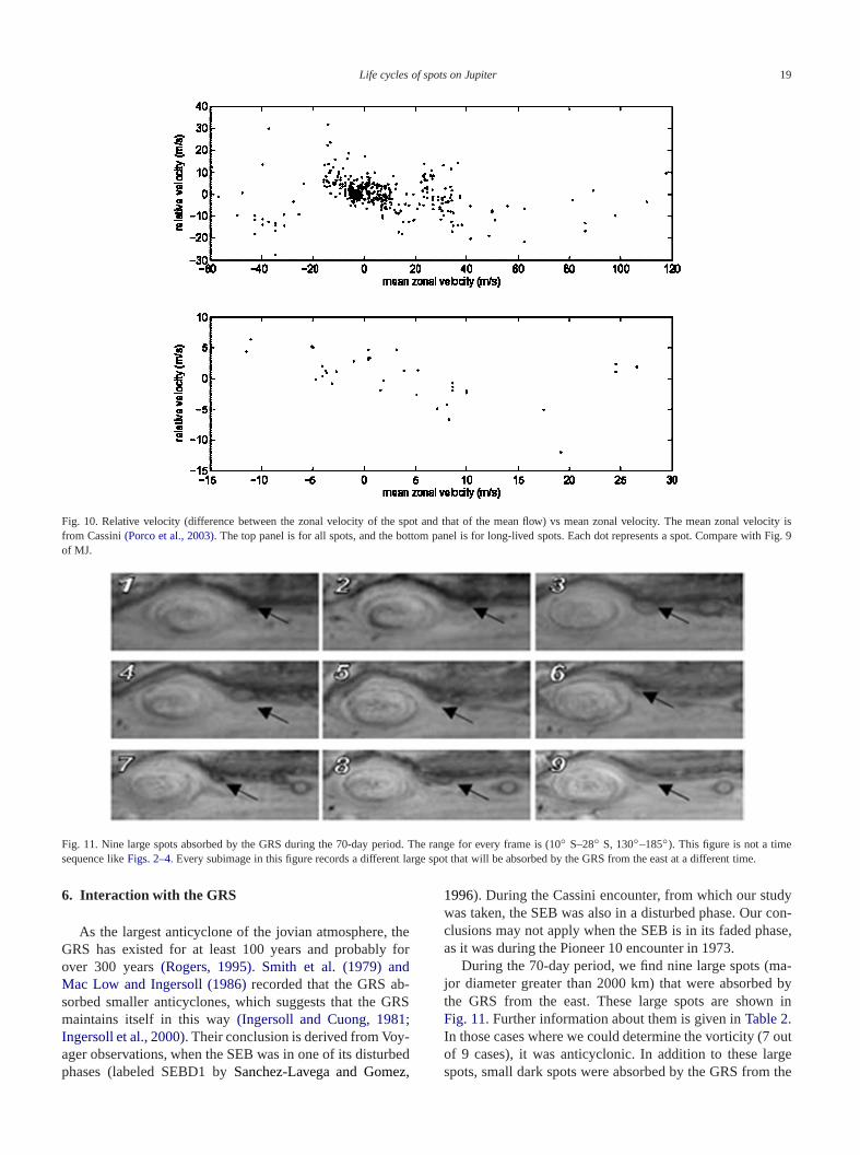
MJ found differences between the vortex speed andmean zonal velocity at the central latitude of each vortextheir Fig. 8). They found that the difference is anti-correlawith the mean zonal velocity.Figure 10is the same as MFig. 9, and shows the relative velocity (difference betwthe zonal velocity of the spot and that of the mean flowthe mean zonal velocity at the center of the spot. Therno obvious anti-correlation (negative slope) between thevariables, except possibly for the long-lived spots (bothalf) if one ignores the three points farthest to the right. Tabsolute value of the slope of the remaining points isthan that of the line in MJ Fig. 9. Our data inFig. 10are nottoo different from those in MJ Fig. 9, considering that thtime base is much longer than ours and we have morefor short-lived spots (top half ofFig. 10).

Fig. 9. Comparison between the latitude distribution of spots and the zonal wind profile. The left panel gives the number of all spots per degree of latitude witha scaling factor 4 (light line) along with the zonal wind profile determined by the feature tracking method (heavy line). The right panel is same as the left panelexcept for long-lived spots and scaling factor 20.

Life cycles of spots on Jupiter 19

ity iig. 9

e.

Fig. 10. Relative velocity (difference between the zonal velocity of the spotand that of the mean flow) vs mean zonal velocity. The mean zonal velocsfrom Cassini(Porco et al., 2003). The top panel is for all spots, and the bottom panel is for long-lived spots. Each dot represents a spot. Compare with Fof MJ.

Fig. 11. Nine large spots absorbed by the GRS during the 70-day period. The range for every frame is (10 S–28 S, 130–185). This figure is not a timesequence likeFigs. 2–4. Every subimage in this figure records a different large spot that will be absorbed by the GRS from the east at a different tim

thefor

-RS

;-rbedz,

dycon-se,

a-d byn in

outrge

the

6. Interaction with the GRS

As the largest anticyclone of the jovian atmosphere,GRS has existed for at least 100 years and probablyover 300 years(Rogers, 1995). Smith et al. (1979) andMac Low and Ingersoll (1986)recorded that the GRS absorbed smaller anticyclones, which suggests that the Gmaintains itself in this way(Ingersoll and Cuong, 1981Ingersoll et al., 2000). Their conclusion is derived from Voyager observations, when the SEB was in one of its distuphases (labeled SEBD1 bySanchez-Lavega and Gome

1996). During the Cassini encounter, from which our stuwas taken, the SEB was also in a disturbed phase. Ourclusions may not apply when the SEB is in its faded phaas it was during the Pioneer 10 encounter in 1973.

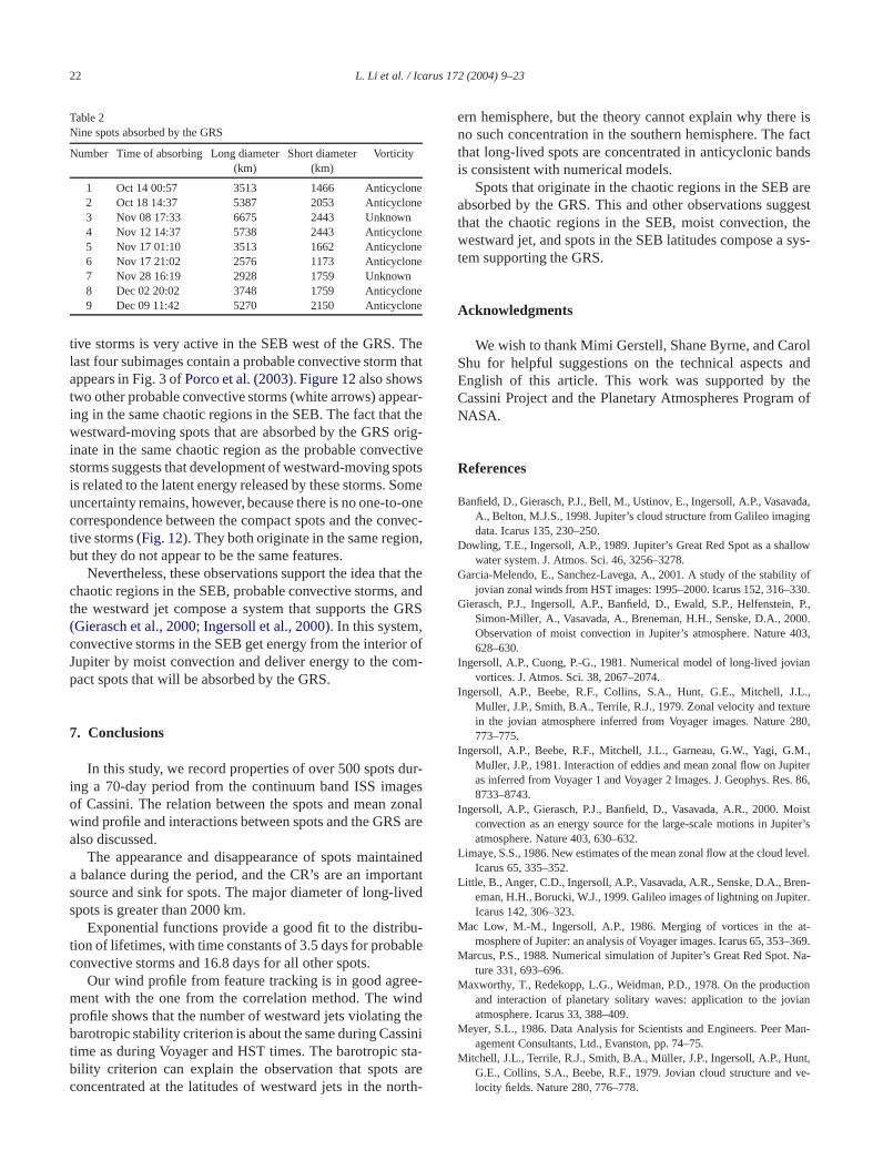
During the 70-day period, we find nine large spots (mjor diameter greater than 2000 km) that were absorbethe GRS from the east. These large spots are showFig. 11. Further information about them is given inTable 2.In those cases where we could determine the vorticity (7of 9 cases), it was anticyclonic. In addition to these laspots, small dark spots were absorbed by the GRS from

20 L. Li et al. / Icarus 172 (2004) 9–23

les ofrighrms

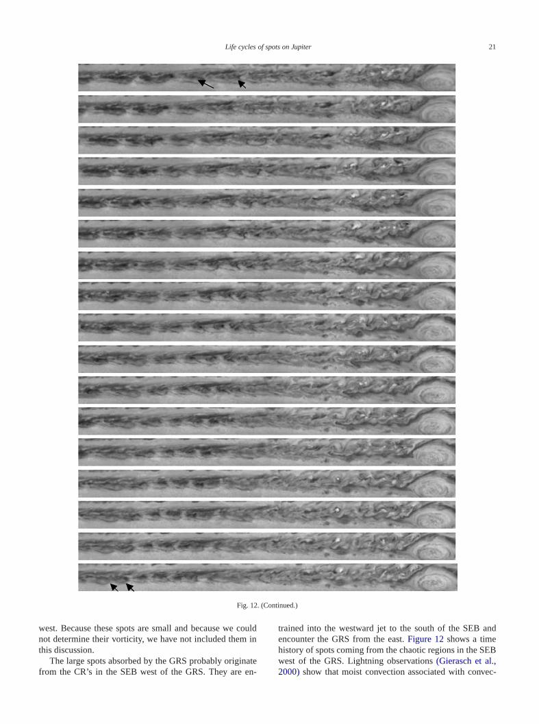
Fig. 12. Spots originating from the chaotic regions in the SEB west of the GRS. The range for every frame is (10 S–24 S, 320–190). Time increasesdown page 1 and then down page 2. The time of the first subimage is Nov10, 2000. The time between two neighboring subimages is 20 h. Two exampcompact spots originating from the SEB and being absorbed finally by the GRS are shown with dark arrows. Tracing these spots from lower left to uppert(backwards in time), we find that all of them come from the chaotic regions inthe SEB west of the GRS. In addition, two bright probable convective stoare shown with white arrows.

Life cycles of spots on Jupiter 21

Fig. 12. (Continued.)

couin

nateen-

and

EB,ec-

west. Because these spots are small and because wenot determine their vorticity, we have not included themthis discussion.

The large spots absorbed by the GRS probably origifrom the CR’s in the SEB west of the GRS. They are

ldtrained into the westward jet to the south of the SEBencounter the GRS from the east.Figure 12shows a timehistory of spots coming from the chaotic regions in the Swest of the GRS. Lightning observations(Gierasch et al.2000)show that moist convection associated with conv

22 L. Li et al. / Icarus 172 (2004) 9–23

ee

eee

ee

hetha

ear-t theorig-ctivepotsom-onnven,

at thandGRS,r ofom-

ur-gesonaare

ainertantved

u-ble

e-indthesinista-arerth-

re isfactnds

aregestthesys-

rolandhem of

ada,g

llow

ty of330., P.,00.403,

ian

.L.,ure280,

M.,piters. 86,

oistiter’s

level.

ren-iter.

t-9.

. Na-

tionian

n-

nt,ve-

Table 2Nine spots absorbed by the GRS

Number Time of absorbing Long diameter Short diameter Vorticity(km) (km)

1 Oct 14 00:57 3513 1466 Anticyclon2 Oct 18 14:37 5387 2053 Anticyclon3 Nov 08 17:33 6675 2443 Unknown4 Nov 12 14:37 5738 2443 Anticyclon5 Nov 17 01:10 3513 1662 Anticyclon6 Nov 17 21:02 2576 1173 Anticyclon7 Nov 28 16:19 2928 1759 Unknown8 Dec 02 20:02 3748 1759 Anticyclon9 Dec 09 11:42 5270 2150 Anticyclon

tive storms is very active in the SEB west of the GRS. Tlast four subimages contain a probable convective stormappears in Fig. 3 ofPorco et al. (2003). Figure 12also showstwo other probable convective storms (white arrows) apping in the same chaotic regions in the SEB. The fact thawestward-moving spots that are absorbed by the GRSinate in the same chaotic region as the probable convestorms suggests that development of westward-moving sis related to the latent energy released by these storms. Suncertainty remains, however, because there is no one-tocorrespondence between the compact spots and the cotive storms (Fig. 12). They both originate in the same regiobut they do not appear to be the same features.

Nevertheless, these observations support the idea thchaotic regions in the SEB, probable convective storms,the westward jet compose a system that supports the(Gierasch et al., 2000; Ingersoll et al., 2000). In this systemconvective storms in the SEB get energy from the interioJupiter by moist convection and deliver energy to the cpact spots that will be absorbed by the GRS.

7. Conclusions

In this study, we record properties of over 500 spots ding a 70-day period from the continuum band ISS imaof Cassini. The relation between the spots and mean zwind profile and interactions between spots and the GRSalso discussed.

The appearance and disappearance of spots mainta balance during the period, and the CR’s are an imposource and sink for spots. The major diameter of long-lispots is greater than 2000 km.

Exponential functions provide a good fit to the distribtion of lifetimes, with time constants of 3.5 days for probaconvective storms and 16.8 days for all other spots.

Our wind profile from feature tracking is in good agrement with the one from the correlation method. The wprofile shows that the number of westward jets violatingbarotropic stability criterion is about the same during Castime as during Voyager and HST times. The barotropicbility criterion can explain the observation that spotsconcentrated at the latitudes of westward jets in the no

t

eec-

e

l

d

ern hemisphere, but the theory cannot explain why theno such concentration in the southern hemisphere. Thethat long-lived spots are concentrated in anticyclonic bais consistent with numerical models.

Spots that originate in the chaotic regions in the SEBabsorbed by the GRS. This and other observations sugthat the chaotic regions in the SEB, moist convection,westward jet, and spots in the SEB latitudes compose atem supporting the GRS.

Acknowledgments

We wish to thank Mimi Gerstell, Shane Byrne, and CaShu for helpful suggestions on the technical aspectsEnglish of this article. This work was supported by tCassini Project and the Planetary Atmospheres PrograNASA.

References

Banfield, D., Gierasch, P.J., Bell, M., Ustinov, E., Ingersoll, A.P., VasavA., Belton, M.J.S., 1998. Jupiter’s cloud structure from Galileo imagindata. Icarus 135, 230–250.

Dowling, T.E., Ingersoll, A.P., 1989. Jupiter’s Great Red Spot as a shawater system. J. Atmos. Sci. 46, 3256–3278.

Garcia-Melendo, E., Sanchez-Lavega, A., 2001. A study of the stabilijovian zonal winds from HST images: 1995–2000. Icarus 152, 316–

Gierasch, P.J., Ingersoll, A.P., Banfield, D., Ewald, S.P., HelfensteinSimon-Miller, A., Vasavada, A., Breneman, H.H., Senske, D.A., 20Observation of moist convection in Jupiter’s atmosphere. Nature628–630.

Ingersoll, A.P., Cuong, P.-G., 1981. Numerical model of long-lived jovvortices. J. Atmos. Sci. 38, 2067–2074.

Ingersoll, A.P., Beebe, R.F., Collins, S.A., Hunt, G.E., Mitchell, JMuller, J.P., Smith, B.A., Terrile, R.J., 1979. Zonal velocity and textin the jovian atmosphere inferred from Voyager images. Nature773–775.

Ingersoll, A.P., Beebe, R.F., Mitchell, J.L., Garneau, G.W., Yagi, G.Muller, J.P., 1981. Interaction of eddies and mean zonal flow on Juas inferred from Voyager 1 and Voyager 2 Images. J. Geophys. Re8733–8743.

Ingersoll, A.P., Gierasch, P.J., Banfield, D., Vasavada, A.R., 2000. Mconvection as an energy source for the large-scale motions in Jupatmosphere. Nature 403, 630–632.

Limaye, S.S., 1986. New estimates of the mean zonal flow at the cloudIcarus 65, 335–352.

Little, B., Anger, C.D., Ingersoll, A.P., Vasavada, A.R., Senske, D.A., Beman, H.H., Borucki, W.J., 1999. Galileo images of lightning on JupIcarus 142, 306–323.

Mac Low, M.-M., Ingersoll, A.P., 1986. Merging of vortices in the amosphere of Jupiter: an analysisof Voyager images. Icarus 65, 353–36

Marcus, P.S., 1988. Numerical simulation of Jupiter’s Great Red Spotture 331, 693–696.

Maxworthy, T., Redekopp, L.G., Weidman, P.D., 1978. On the producand interaction of planetary solitary waves: application to the jovatmosphere. Icarus 33, 388–409.

Meyer, S.L., 1986. Data Analysis for Scientists and Engineers. Peer Maagement Consultants, Ltd., Evanston, pp. 74–75.

Mitchell, J.L., Terrile, R.J., Smith, B.A., Müller, J.P., Ingersoll, A.P., HuG.E., Collins, S.A., Beebe, R.F., 1979. Jovian cloud structure andlocity fields. Nature 280, 776–778.

Life cycles of spots on Jupiter 23

2002ear

,

-

lt of

A.,.E.,ebe,

gs,oy-

Bel-.,lileon,

soli-

rom

Morales-Juberias, R., Sanchez-Lavega, A., Lecacheux, J., Colas, F.,A comparative study of jovian anticyclone properties from a six-y(1994–2000) survey. Icarus 157, 76–90.

Porco, C.C., 23 colleagues, 2003. Cassini imaging of Jupiter’s atmospheresatellites, and rings. Science 299, 1541–1547.

Rogers, J.H., 1995. The Giant Planet Jupiter. Cambridge Univ. Press, Cambridge, UK.

Sanchez-Lavega, A., Gomez, J.M., 1996. The South Equatorial BeJupiter. I. Its life cycle. Icarus 121, 1–17.

Smith, B.A., Soderblom, L.A., Johnson, T.V., Ingersoll, A.P., Collins, S.Shoemaker, E.M., Hunt, G.E., Masursky, H., Carr, M.H., Davies, MCook II, A.F., Boyce, J., Danielson, G.E., Owen, T., Sagan, C., Be

. R.F., Veverka, J., Strom, R.G., McCauley, J.F., Morrison, D., BrigG.A., Suomi, V.E., 1979. The Jupiter system through the eyes of Vager 1. Science 204, 951–972.

Vasavada, A.R., Ingersoll, A.P., Banfield, D., Bell, M., Gierasch, P.J.,ton, M.J.S., Orton, G.S., Klaasen, K.P., De Jong, E., Breneman, H.HJones, T.J., Kaufman, J.M., Magee, K.P., Senske, D.A., 1998. Gaimaging of Jupiter’s atmosphere: the Great Red Spot, equatorial regioand White Ovals. Icarus 135, 265–275.

Williams, G.P., Yamagata, T., 1984. Geostrophic regimes, intermediatetary vortices and jovian eddies. J. Atmos. Sci. 41, 453–478.

Youssef, A., Marcus, P.S., 2003. The dynamics of jovian white ovals fformation to merger. Icarus 162, 74–93.