Life-cycle effects of age at school start∗

Peter Fredriksson Björn Öckert

Abstract

In Sweden, children typically start compulsory school the year they turn 7. Individuals

born around the new year have about the same date of birth but enter school at different

ages. We exploit this source of exogenous variation to identify effects of age at school

entry on educational attainment and long-run labor market outcomes. Using data for the

entire native population born 1935-55, we find that school entry age raises educational

attainment. We show that the comprehensive school reform (which postponed tracking

until age 16) reduced the effect of school starting age on educational attainment. We also

trace the effects of school starting age on prime-age earnings, employment, and wages.

On average, school starting age only affects the allocation of labor supply over the life-

cycle; prime-age earnings is unaffected, and there is a negative effect on discounted

life-time earnings. But for individuals with low-educated parents, and to some extent

women, we find that prime-age earnings increase in response to age at school start.

JEL-codes: I21, I28, J24, C31Keywords: School starting age, educational attainment, life-time earnings, regression discon-tinuity

1 Introduction

There is an extensive literature on the relationship between age at school start and in-schoolperformance. The results typically indicate that older school starters do better in school.∗This version: March 2013. Fredriksson is affiliated with Stockholm University, the Institute for Evaluation

of Labour Market and Education Policy (IFAU), IZA, and the Uppsala Center for Labor Studies (UCLS). Öckertis affiliated with IFAU, Uppsala University, and UCLS. We thank Olof Åslund, Torsten Persson, Steve Pischke,Roope Uusitalo, two anonymous referees, as well as seminar and conference participants at IUI, SOFI, IFAU,FIEF, NTNU, IIES, the Universities of Copenhagen, Göteborg, Helsinki, Montreal, Växjö, EALE/SOLE, theCEPR conference on "Education and Inequality", and the first EEEPE workshop for valuable comments. Fi-nancial support from the Marcus and Amalia Wallenberg foundation and Handelsbanken is gratefully acknowl-edged.

1

But these results are hard to interpret since older school starters are also older when schoolperformance is measured. In contrast to much of the literature, this paper focuses on thelong-run effects of school entry age.

More precisely, we ask the question: How does school starting age affect educationalattainment and long-run labor market outcomes? To answer this question we exploit ex-ogenous variation in school starting age due to month of birth and the school entry cut-offdate (the 1st of January). This implies a regression-discontinuity design which we apply tounique Swedish administrative data. The data pertain to the entire native Swedish populationborn between 1935 and 1955. The data set includes earnings information spanning the entirecareer of these cohorts as well as educational attainment at age 40-50.

Swedish data are particularly apt for examining the issues addressed in this paper. Oneadvantage is that the compulsory schooling law requires individuals to complete a minimumnumber of years of education, independently of when they start. Moreover, grade retentionor advancement is rarely practiced in Sweden. These two features facilitate the identificationof the school starting age effect, since the effect is not contaminated by the variation in yearsof compulsory schooling. Things are different in, e.g., the U.S. context, where the schoolleaving age legislation implies that season of birth has an impact on years of compulsoryschooling (Angrist and Krueger 1991).

Another advantage is that we have information on earnings from 1960 until 2009. Thus,we can analyze earnings outcomes throughout the career for most cohorts. Previous analysesof school entry age on earnings have either used data for a single point in time for severalcohorts (Fredriksson and Öckert 2005 and Dobkin and Ferreira 2010) or panel data coveringthe ages 24-35 (Black et al. 2011). Relative to Black et al. (2011) our value added is that weextend the analysis beyond age 35. In particular, we estimate the effect of school entry ageon prime-age (25-54) earnings for all cohorts. Moreover, some cohorts are observed beyondthe nominal retirement age (65) and we calculate the effect on actual life-time earnings. Theanalysis of earnings outcomes throughout the career is the first major value added of thepaper.

A final advantage or our data is that they span cohorts who attended school in differentsystems. The older cohorts went to school in a selective system with early tracking; theyounger cohorts attended a comprehensive system where students were held together. Thiscompulsory school reform was phased in in different parts of the country (Meghir and Palme2005; Holmlund 2007). This setting lends itself to a differences-in-differences analysis whichcompares the effect of school starting age on educational attainment across school systemsholding cohort constant. This is the second major value added of our paper. Our evidence on

2

this point should be more credible than the evidence reported in Bedard and Dhuey (2006)who compared age effects across countries while children are still in school.1

Throughout the paper we focus on long-run outcomes. We thus circumvent the fundamen-tal identification problem which occurs when children are still in school. With informationon adult outcomes, observed at a given time-point, it is possible to hold age at observationconstant and still identify school starting age via the discontinuity around the school entrycut-off.2

Our paper is related to an extensive literature. The vast majority of studies examine in-school outcomes (see Stipek 2002 for a survey). For reasons explained above it is hard tointerpret the results in this literature as the effect of school starting age.3 There is a morerecent economics literature on how season of birth and school starting age affect long-runoutcomes. The first paper in this vein is Angrist and Krueger (1992) who examined howseason of birth affects educational attainment. The paper most similar to ours is the recentanalysis by Black et al. (2011). They conclude that the long-run effects on education andearnings are modest.

While we credibly estimate the long-run impacts of school entry age, we have less tooffer on the precise mechanism. When it comes to the relationship between age at schoolstart and skill acquisition, the literature has emphasized two kinds of mechanisms: one due toabsolute maturity – learning in a school environment is more/less effective at certain ages –and another due to relative maturity – being the oldest in class gives an early advantage whichmay persist in the longer run.4 The variation we are using captures both of these mechanismsand we cannot separate them. Note that, even if only relative maturity at school start isrelevant, it is likely that the effects will persist for some time. In systems where children aretracked early on it is more likely that early advantages will persist; see Bedard and Dhuey(2006). Since we do not disentangle relative and absolute school starting age effects, our

1Also, see Muhlenweg and Puhani (2010) for suggestive evidence on the impact of tracking on school entryage effects.

2Having said this, we recognize that age at crucial stages of selection may still be important for long-runoutcomes. We attribute such effects to school starting age since if children had not started school at differentages, age at the crucial stage of selection would not have varied.

3There are some recent attempts to separate school starting age from age at test. These attempts typicallyrely on functional form assumptions to separate age at observation from age at school start. Two examples areDatar (2006) and Elder and Lubotsky (2009).

4Absolute maturity include: theories of "critical periods" where the brain is especially sensitive to specificexperiences (Shonkoff and Phillips 2000); and theories emphasizing that young children lack the maturity tolearn complicated things in a school environment. Relative maturity include: a theory based on peer quality,where younger children may benefit from being surrounded by older and more able peers; and evidence frompsychology where older children respond to early encouragement by pushing to perform even better in thefuture.

3

evidence do not speak to the wider policy question of whether school start should be pushedearlier or later.

Our empirical strategy mimics the following decision problem. Consider a parent whosechild is born in December. The parent may opt for the normal school start, in which case thechild will be the youngest in class, or it may hold back the child a year. If the child is heldback, it will have an initial advantage which may result in higher attainment in the longerrun. But holding back the child a year, implies forgone earnings for given age. These initiallosses should be traded off with the potential for subsequent earnings gains in the future. Inour empirical work, we estimate the effects of school starting age on the age-earnings profileand thus provide a sense of the magnitudes of initial losses and subsequent gains (if any).

We find that starting school at older age raises educational attainment. The school start-ing age effects are more pronounced in the school system featuring earlier tracking. Onaverage, school entry age mainly affect the timing of labor supply over the life-cycle; prime-age earnings is unaffected, and there is a negative effect on discounted life-time earnings.For individuals with low-educated parents and, to some extent, women, we document a pos-itive effect on prime-age earnings. These effects are mostly driven by higher probability ofworking among those who start school at older age.

2 Compulsory schooling in Sweden

Compulsory school starts the year the children turns 7 which implies a school entry cut-off date on the 1st of January. Most parents adhere to the rule; moreover, retention andadvancement is rarely practiced in Sweden. Data for the 1960s (relevant for the cohorts bornin the 1950s) suggest that half of those finishing late (only 3.6 % of the population) wereretained during compulsory school.

The cohorts we are studying (the cohorts born 1935-55) were exposed to two differentschool systems. The older cohorts (basically those born 1935-1945) lived under a ratherselective system. In this system, 7 or 8 years of schooling were mandatory, local authori-ties determined the curriculum, and strict ability tracking was implemented in grade 5 or 7.Children in different tracks went to different schools; children in the lower tracks had scantopportunities to pursue further education.

In 1950, the parliament decided to introduce a 9-year "comprehensive school" graduallyacross the country. Whether a municipality (or city community) should implement the reformwas determined by the National Board of Education, after an application by the municipality

4

(or the city community).5 The reform abolished strict tracking and featured a nationally de-termined curriculum. There was still some tracking in lower secondary school. Importantly,however, students in different tracks attended the same school. Moreover, choosing the lowertrack did not imply that further educational opportunities were closed. The gradual introduc-tion of the comprehensive school mainly affected the cohorts born between 1945 and 1955(Holmlund 2007). In the 1945 cohort, 2% attended the new comprehensive school; in the1955 cohort this share had increased to 98%.

The older cohorts in our data were also exposed to some reform. In particular, compulsoryschool could be extended from 7 to 8 years on the decision of the local authorities. This is areform within the same basic structure of the school system, and hence not as radical as thecomprehensive school reform.

The time-period we study is a period where pre-school education was not available. In1950, the number of child-care slots could accommodate 1.4% of the population aged 1-5. The time-period features a substantial rise in educational attainment. The probability ofhaving at least 2 years of college education increased from 9% (cohort born 1935) to 17%(1955 cohort).

3 Empirical strategy

For an individual i, in cohort c, the outcome equation of interest is

yic = αc +βSSAic + f kc (Mic)+ εic, (1)

where SSA denotes age at school start, M month of birth, and the outcomes considered arelong-run educational and labor market outcomes. αc denotes a cohort fixed effect, where wedefine a cohort as running from July to June rather than over year of birth. The school entrycut-off is thus in the middle of a cohort defined in this way. f k

c (Mic) denotes a polynomialcontrol function (of order k) in the “assignment variable” (month of birth) which is interactedwith the cut-off and (potentially) by cohort. Month of birth is normalized to zero around theschool entry cut-off and thus Mic = {−5.5, ...,5.5}.

Since individuals may be selected on (projected) academic ability when starting school,SSA is potentially endogenous. We instrument it using the school entry cut-off. Define thetreatment indicator A f ter as

A f teric = I(Mic > 0) (2)

5City communities are parts of municipalities in the big-cities.

5

Since M is normalized to zero at the cut-off, A f ter = 1 for individuals born January to Juneand 0 otherwise. The first stage equation thus is

SSAic = δc + γA f teric +gkc(Mic)+νic (3)

and the reduced formyic = θc +λA f teric +hk

c(Mic)+µic (4)

In equations (3)-(4): δc, and θc are cohort fixed effects; and gkc(Mic) and hk

c(Mic) are controlfunctions defined in the same way as f k

c (Mic). The control functions take care of any smoothunderlying relationship between month of birth and the outcome of interest. Within cohort,the control functions also hold age at observation constant. Identification is achieved by thediscrete jump in school starting age at the cut-off. In particular, children born on each side ofthe new year have about the same date of birth but differ in their school starting age by almosta year. Since the rule is not completely binding, this is a fuzzy Regression Discontinuity (RD)design.

The assignment variable is discrete; thus, we have to rely on a parametric control function.In these situations, Lee and Card (2008) recommend clustering the standard errors on thediscrete values of the assignment variable. We follow their recommendation.

Another complication is that we do not observe SSA and the outcomes in the same dataset. This is thus an example of two-sample instrumental variables (Angrist and Krueger1992). Inoue and Solon (2010) note that the best way to deal with this issue is to view it as agenerated regressors problem and use the method proposed by Murphy and Topel (1985) tocorrect the standard errors. We follow this approach.

The validity of the instrument can be examined in a number of ways. The most straightfor-ward way is to examine whether predetermined characteristics are related to the instrument.But we also check whether the distribution of births around the discontinuity is smooth (seeMcCrary 2008). In section 5 and in the Appendix we discuss various tests of instrumentvalidity.

The two-stage least squares strategy relies on the assumption that there are no otherchanges around the cut-off that affects outcomes. A source of concern is that educationalreforms typically pertain to year of birth rather than our July/June definition of cohorts. Theeducational reforms, described in Section 2, added 1-2 years of compulsory education. Thisis a potential problem since it may mechanically raise educational attainment among thoseborn after the cut-off during the reform year.

6

Reform status varies by place of residence and year of birth. Hence we can constructindicators for whether a given individual was subjected to reform. Since place of residencemay be endogenous to the reform, we assign reform status on the basis of parish of birth andyear of birth. This strategy allows us to address the potential problem caused by the reformsit two ways: first, we hold reform status and birth parish constant, thus controlling for anymechanical effect affecting our key estimate; second, we exclude years when a particularparish reformed. As it turns out it does not matter which approach we use, so the first strategyis our main strategy.

4 Data

The data mainly come from administrative records. The administrative data originate fromStatistics Sweden and cover the entire population born in Sweden 1935-55.6 To these datawe have matched information on annual earnings, educational attainment, and wages, as wellas information on education and employment for the biological parents. Information on yearand month of birth originate from birth records and do not suffer from measurement error.All wage and earnings data are in SEK 2009 values.

The earnings data are available 1960-66, 1968, 1970-71, 1973, 1975-76, 1979-80, 1982,1985-2009. Between 1960 and 1966 the earnings data are available for a 10% sample (in-dividuals born on the 5th, 15th, and 25th of each month). From 1968 and onwards they areavailable for the entire population. These data span the entire labor market careers of mostcohorts. Individuals in the oldest cohort are observed when they are aged 25-74; individualsin the youngest cohort are observed when they are aged 16-54.

The wage data are available during 1985-2009 and stem from the so-called Wage reg-ister. Monthly wages are measured in full-time equivalents and thus analogous to hourlywages; they are collected for those who are employed on a particular day of measurement(in September-November). Using the mapping between wages and earnings for cells definedby the interactions between gender, age, and education we construct indicators of whetherindividuals are (full-time) employed; the Appendix describes this procedure more fully.

Information on educational attainment is available from the Censuses conducted in 1960,1970 and 1990, and from the Educational register from 1985 and onwards. As the generalrule we use information when the individuals are aged 45. For the individuals under study,we mainly use the information between 1985 and 2000 and for the parents we use the 1960

6We exclude all immigrants since they lack reliable information on date of birth, school starting age, andyears of schooling.

7

or 1970 censuses. A small fraction of the sample (2.96%) have missing information on eitherthe mother or the father; for these individuals we have no information on the education of theparent. We translate educational attainment to years of schooling using information on thetypical years of schooling associated with a given attainment level.

School starting age is not reported in our main data set. Instead we use data from “Evalua-tion Through Follow-up” (ETF), a project run by the Department of Education at the Univer-sity of Göteborg (see Härnquist 2000). These data, inter alia, contain information for a 10%sample of the cohort born 1948 (individuals born on the 5th, 15th, and 25th of each month).We estimate the relation between school starting age and birth month in the ETF-data andthen predict school starting stage for all cohorts in the main data set.

5 Validity of the instrument

A threat to the validity of the RD design is if (certain) parents systematically time their birthswith respect to the cut-off. Figures 1 and 2 present two pieces of evidence demonstratingthat there is no evidence of such behavior. Figure 1 shows that there is no suspect jumpin the number of births around the discontinuity. Figure 2 shows that parental educationis balanced at the cutoff; the estimated discontinuity is 0.013 years with a standard error of0.014. Moreover, in the Appendix we show that these conclusions hold up when we use morefinely grained birth information, which is not available in the main data.

Table 1 presents further evidence by examining whether gender, parental education, andparental employment are balanced around the cut-off.7 To facilitate readability all estimatedcoefficients (and standard errors) are multiplied by 100.8

Column (1) presents the results of regressing the instrument on parental education andgender. In column (2) we add parental employment to the regression. By conditioning onparental employment we loose an additional 12% of the sample, which is why we presenttwo sets of regression results.9 Column (3) adds the educational reform controls.

The p-values, reported in the second row from the end, range from 0.533 to 0.760. Thus,we do not reject the hypotheses that the covariates are unrelated to the instrument. Column (4)

7All these characteristics are highly relevant for all outcomes. For instance, mother’s who have an additionalyear of education have children who on average have 0.23 additional years of education (t-ratio: 63.6).

8The estimate on Female in the first row of column 1 thus says that the probability of being born after thecutoff is 0.005 percentage points higher for females than for males.

9Information on parental employment comes from the censuses in 1960 and 1965. In the strict sense, it is notpre-determined with respect to child birth. We think this is a minor problem. Nevertheless, this is an additionalreason for presenting separate regressions.

8

Figure 1. Distribution of births by birth month

Note: The figure shows the distribution of births by birth month among natives who are born between July 1935and June 1955

Figure 2. Parental education by month of birth

Notes: Parental years of schooling is defined as the maximum of the education of the father or the mother. Dis-continuity at cut-off: 0.013 (standard error: 0.014). The solid line depicts the school entry cut-off. Regressionlines are 2nd order polynomials fitted separately to the individual data on each side of the cut-off. We controlfor cohort and educational reform (see section 2).

9

Table 1. Balancing of covariates

Dependent variable: After cut-off p-value of(Coefficient/SE:s mult. by 100) bivariate correlation(1) (2) (3) (4)

Female 0.005 0.012 0.012 0.614(0.021) (0.024) (0.024)

Mother’s education 0.012 0.013 0.016 0.211(0.008) (0.009) (0.010)

Father’s education -0.002 -0.002 -0.002 0.670(0.005) (0.005) (0.007)

Mother employed – -0.007 -0.012 0.856(0.029) (0.030)

Father employed – 0.016 0.019 0.763(0.065) (0.065)

Educational reform controls√ √

Month of birth controls2nd order

√ √ √ √

Interacted w. cutoff√ √ √ √

p-value of F-test 0.533 0.760 0.651 –# individuals 1,978,242 1,733,070 1,732,987 1,732,987

Notes: Coefficients and standard errors are multiplied by 100 to facilitate readability. The regressions are basedon individuals born July 1935 to June 1955. They include (20) cohort fixed effects where a cohort includeindividuals born July/June. The educational reform controls are dummies for the two reforms described insection 2 and birth parish FE:s. Results in column (4) come from separate regressions of the covariate, reportedin each row, on the instrument. Standard errors, shown in parentheses, allow for clustering (240 clusters) on thediscrete values of the assignment variable.

10

adds more evidence on this point by examining the bivariate relation between each individualcharacteristic and the instrument. Each row in column (4) reports the p-value of a t-testobtained by regressing the characteristic in question on the instrument. Again, we do notreject the hypothesis that each individual characteristic is unrelated to the instrument.

The regression results are based on controlling for a 2nd order polynomial in birth monthinteracted with the cut-off.10 A specification with a first order polynomial (interacted withthe cut-off) is inferior to the specification with the 2nd order polynomial. With a linearinteracted control function we reject the hypothesis of no relation between the instrumentand the covariates. Adding higher-order polynomials do not change the results. Addinginteractions between cohort and the 2nd order (interacted) polynomial do not change theresults either. We therefore conclude that baseline covariates are unrelated to the instrument,given that we control sufficiently flexibly for month of birth.

Figure 3 illustrates the relation between age at school start and birth month in the ETF-data. There is a substantial jump in school starting age around the cut-off. Individuals bornjust after the school entry cut-off, start when they are 0.86 years older than those born justbefore the cut-off (the t-ratio is 49.2).

The reason for the strong relationship between SSA is that it was relatively uncommonto start school early or late, even for those born around the cut-off. On average only 2.0%of the individuals started early while 3.3% started late. Even though early starts were morecommon among individuals born in January (7%), and late starts more common among thoseborn in December (8%), the overwhelming majority of the individuals born around the cutoffstart at the normal time.

Figure 4 shows the probability of starting early and late by birth month and gender. Itis more likely that boys start late. The probability that a boy born in December starts late is9.1%; the corresponding number for girls is 5.6%. This gender difference arguably reflectsless maturity among boys around school start. If this is the correct interpretation, one wouldexpect the probability of starting early to be lower among boys. However, there is no suchpattern in the data. In fact, the probability that boys born in January start early is 6.8%; thecorresponding number for girls is 6.7%. A similar pattern is true for February (boys 5.4%;girls 5.1%). But March is more in line with expectation, i.e., lower for boys (2.3%) than forgirls (3.6%). The probability of starting early among boys born just after the cut-off appearsto be too high, both relative to boys born slightly later (i.e. March-June) and relative togirls born just after the cut-off. Parents (and, perhaps, school teachers) appear to be overly

10Table 2 below examines the sensitivity of the results to the specification of the control function.

11

Figure 3. School starting age and birth month

Notes: The figure is based on individuals born 1948 who are included in the ETF-data (those born on the 5th,15th, and 15th each month). Discontinuity at threshold: 0.86 (standard error: 0.02). Regression lines are 2ndorder polynomials fitted separately to the individual data on each side of the cut-off. The solid vertical linedepicts the school entry cut-off. Those just to the left of the threshold are born in December 1948 and those justto the right of the threshold are born in January 1948. In constructing this figure we have assumed that there isno underlying trend in SSA.

optimistic about the school performance of boys born just after the cut-off.This reasoning suggest that we would ideally like to allow for differential effects of start-

ing early and late. Unfortunately, we cannot do this since we only have one cut-off. Ourinstrumental variables results thus reflect the combined effect of starting early or late.

6 Descriptive analysis

We illustrate the gist of our results by a set of graphs. In these graphs we relate the outcomesto the school entry law and month of birth. Figure 5 presents the aggregate picture by showinghow education and earnings at various ages are related to month of birth. The top-left graphpertains to years of schooling; the top-right graph to earnings at age 18; the bottom-left graphto earnings at age 35; and the bottom-right graph to earnings at age 62. We measure age-specific earnings relative to average prime-age earnings (age 25-54) per cohort. Notice thatthis is just a normalization to facilitate interpretation.

Figure 5 shows that individuals born just after the school-entry cut-off have (significantly)higher educational attainment. The jump at the cut-off amounts to an increase in years of

12

Figure 4. Early and late school starts by birth month and gender

Notes: The graphs are based on individuals born 1948 who are included in the ETF-data (those born on the 5th,15th, and 15th each month). The solid vertical lines depict the school entry cut-off. Those just to the left of thisthreshold are born in December 1948; those just to the right of the threshold are born in January 1948.

schooling of 0.14 years.Remaining three figures show earnings effects at various stages of the life-cycle. The top-

right graph illustrates that individuals born just after the cut-off have lower earnings at age 18.Individuals born just after the cut-off enter the labor market almost a full year later and havemore education. Both of these factors imply less experience for given age, which contributesto lower earnings early on in the career. Earnings at age 35, on the other hand, is unrelated tothe expected school starting age; see the bottom-left graph. The earnings premium associatedwith the increase in education seems to be balanced by the loss of experience associated withstarting school at an older age. The bottom-right graph shows that earnings close to retirementis higher for those born just after the cut-off; the increase amounts to 4% of average prime-ageearnings.

Hidden in the averages shown in Figure 5 there is substantial heterogeneity. Figure 6 andFigure 7 examine heterogeneous effects on education and prime-age earnings respectively.

Figure 6 shows the relationship between educational attainment and month of birth forvarious groups. The top panel presents this relationship separately by gender. Being bornjust after the cut-off has a bigger effect on education for women than for men: the jump at thecut-off corresponds to 0.16 years of schooling for females and 0.11 years for males. Malesborn in January and February do not gain as much by being born after the cut-off as theirfemale counterparts. We think the explanation for this fact lies in the behavior illustrated inFigure 4 where it seems that parents are overly optimistic about the school performance ofboys born in January and February. To the extent that parents err in their judgment, boys

13

Figu

re5.

Edu

catio

nan

dag

e-sp

ecifi

cea

rnin

gsby

mon

thof

birt

h

Not

es:

The

top-

left

grap

hsh

ows

year

sof

educ

atio

nby

birt

hm

onth

.D

isco

ntin

uity

atcu

t-of

f:0.

137

(sta

ndar

der

ror:

0.01

8).

The

top-

righ

tgra

phpe

rtai

nsto

earn

ings

atag

e18

.D

isco

ntin

uity

atcu

t-of

f:-0

.040

(sta

ndar

der

ror:

0.00

4).

The

botto

m-l

eftg

raph

pert

ains

toea

rnin

gsat

age

35.

Dis

cont

inui

tyat

cut-

off:

-0.0

01(s

tand

ard

erro

r:0.

003)

.T

hebo

ttom

-rig

htgr

aph

pert

ains

toea

rnin

gsat

age

62.

Dis

cont

inui

tyat

cut-

off:

0.04

2(s

tand

ard

erro

r:0.

008)

.T

heso

lidve

rtic

allin

esde

pict

the

scho

olen

try

cut-

off.

Reg

ress

ion

lines

are

2nd

orde

rpo

lyno

mia

lsfit

ted

sepa

rate

lyto

the

indi

vidu

alda

taon

each

side

ofth

ecu

t-of

f.E

stim

ates

atag

e18

are

wei

ghte

dto

adju

stfo

ra

low

ersa

mpl

ing

prob

abili

tydu

ring

1960

-66.

Age

-spe

cific

earn

ings

isde

fined

rela

tive

topr

ime-

age

earn

ings

perc

ohor

t.T

hefig

ures

are

base

don

coho

rts

born

July

1935

toJu

ne19

55.W

eco

ntro

lfor

coho

rtan

ded

ucat

iona

lref

orm

(see

sect

ion

2)th

roug

hout

.

14

who start early are particularly hurt by being the youngest in class. The manifestation of thisis that January and February born men have lower attainment than we would expect, bothrelative to females and relative to men born March to June.

The lower panel presents the relationship between years of schooling and month of birthby the education of their parents. Individuals born to low-educated parents (both parentshave at most 7 years of education) and just after the cut-off have an additional 0.18 years ofeducation relative to those born just before the cut-off. For individuals with high-educatedparents (at least one parent have more than 7 years of education), the jump at the cut-offcorresponds to 0.12 years of schooling. Again, there seems to be something particular goingon among individuals born in January and February to high-educated parents. We thinkthe likely explanation is the same as for the gender difference. The probability of startinglate is roughly the same for children born in December across family background (8.3%for individuals with low-educated parents; 7.0% for individuals with high-educated parents).However, the probability of starting early for individuals born in January to high-educatedparents is substantially higher (7.6%) than among individuals born in January to low-educatedparents (4.6%). It seems that highly educated parents tend to overestimate the performanceof their January and February born children, which may have negative consequences for theireducational outcomes.

Figure 5 showed that school starting age mainly affects the allocation of life-time laborsupply for the average worker: on average, earnings during prime-age is unaffected by theschool entry cut-off. Again, there is substantial heterogeneity hidden in the average; seeFigure 7. And, qualitatively, the difference across groups line-up well with the differentialimpact on education across groups.

The top-left graph shows that women who are born just after the school entry cut-off havehigher earnings at age 35. The effect amounts to 1.1% of prime-age earnings (with a standarderror of 0.4%). The top-right graph shows the corresponding relationship for men. For men,being born after the school entry cut-off implies a loss of 0.6% (standard error 0.3%). Forindividuals with low-educated parents, the effect of being born just after the school entrycut-off is positive and amounting to 1.0% (standard error 0.5%), while there is no effect forindividuals with high-educated parents (the estimate is -0.4% with a standard error of 0.3).

For men and those with high-educated parents, the underlying relationship between birthmonth and outcomes to the right of the discontinuity suggests that the impact on education iskey to understand the effect on earnings at age 35. The downward jump at the discontinuityfor men, in particular, is accounted for by a loss of a year of potential experience for thoseborn just after the cut-off. In general, a year of experience has a bigger effect on the earnings

15

Figu

re6.

Edu

catio

nby

mon

thof

birt

h,he

tero

gene

ous

effe

cts

Not

es:

The

top-

left

grap

hsh

ows

educ

atio

nby

birt

hm

onth

for

wom

en;

disc

ontin

uity

atcu

t-of

f:0.

162

(s.e

.:0.

019)

.T

heto

p-ri

ghtg

raph

pert

ains

tom

en;

disc

ontin

uity

atcu

t-of

f:0.

112

(s.e

.:0.

024)

.T

hebo

ttom

-lef

tgra

phpe

rtai

nsto

indi

vidu

als

with

low

-edu

cate

dpa

rent

s(d

isco

ntin

uity

atcu

t-of

f:0.

181

(s.e

.:0.

022)

)and

the

botto

m-r

ight

grap

hto

indi

vidu

als

with

high

-edu

cate

dpa

rent

s(d

isco

ntin

uity

atcu

t-of

f:0.

121

(s.e

.:0.

020)

).T

heso

lidve

rtic

allin

esde

pict

the

scho

olen

try

cut-

off.

Reg

ress

ion

lines

are

2nd

orde

rpol

ynom

ials

fitte

dse

para

tely

toth

ein

divi

dual

data

onea

chsi

deof

the

cut-

off.

The

resu

ltsar

eba

sed

onco

hort

sbo

rnJu

ly19

35to

June

1955

.We

cont

rolf

orco

hort

and

educ

atio

nalr

efor

m(s

eese

ctio

n2)

thro

ugho

ut.

16

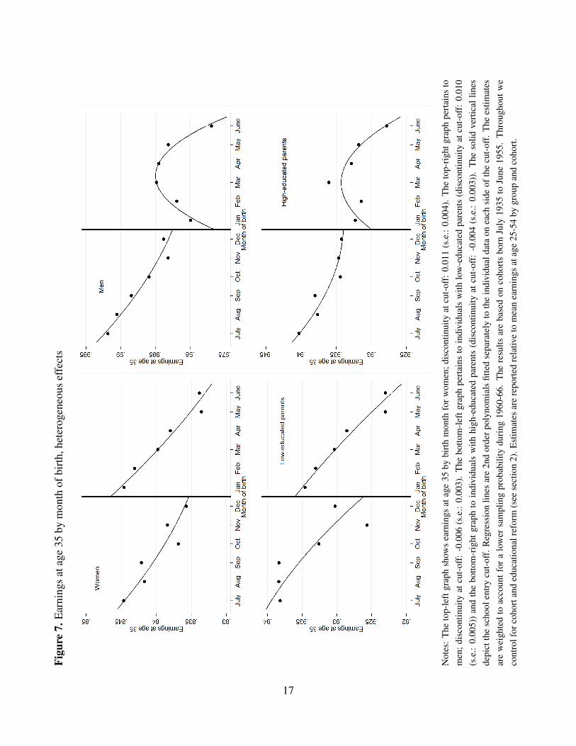
Figu

re7.

Ear

ning

sat

age

35by

mon

thof

birt

h,he

tero

gene

ous

effe

cts

Not

es:

The

top-

left

grap

hsh

ows

earn

ings

atag

e35

bybi

rth

mon

thfo

rw

omen

;dis

cont

inui

tyat

cut-

off:

0.01

1(s

.e.:

0.00

4).

The

top-

righ

tgra

phpe

rtai

nsto

men

;dis

cont

inui

tyat

cut-

off:

-0.0

06(s

.e.:

0.00

3).

The

botto

m-l

eftg

raph

pert

ains

toin

divi

dual

sw

ithlo

w-e

duca

ted

pare

nts

(dis

cont

inui

tyat

cut-

off:

0.01

0(s

.e.:

0.00

5))

and

the

botto

m-r

ight

grap

hto

indi

vidu

als

with

high

-edu

cate

dpa

rent

s(d

isco

ntin

uity

atcu

t-of

f:-0

.004

(s.e

.:0.

003)

).T

heso

lidve

rtic

allin

esde

pict

the

scho

olen

try

cut-

off.

Reg

ress

ion

lines

are

2nd

orde

rpol

ynom

ials

fitte

dse

para

tely

toth

ein

divi

dual

data

onea

chsi

deof

the

cut-

off.

The

estim

ates

are

wei

ghte

dto

acco

untf

ora

low

ersa

mpl

ing

prob

abili

tydu

ring

1960

-66.

The

resu

ltsar

eba

sed

onco

hort

sbo

rnJu

ly19

35to

June

1955

.T

hrou

ghou

twe

cont

rolf

orco

hort

and

educ

atio

nalr

efor

m(s

eese

ctio

n2)

.Est

imat

esar

ere

port

edre

lativ

eto

mea

nea

rnin

gsat

age

25-5

4by

grou

pan

dco

hort

.

17

of men than on the earnings of women.In Section 8 we probe deeper into the earnings results, by, inter alia, investigating whether

the positive effects for women and those with low-educated parents are due to improvedemployment prospects or wage increases.

7 The effect of SSA on educational attainment

This section presents a collection of evidence on the importance of age at school start forschooling. Section 7.1 contains specification analyses; Section 7.2 reports results by gen-der, parental education, and cohort; Section 7.3 examines whether the comprehensive schoolreform reduced the importance of initial advantage by postponing tracking.

7.1 Specification analysis

Here we present reduced form evidence on the importance of month of birth for educationalattainment. The main question is how flexibly we need to control for the underlying relation-ship between birth month and education in order to obtain reliable estimates. Table 2 presentsthe results.

Column (1) shows the results of a baseline specification including a 2nd order polyno-mial in birth month (interacted with the cut-off): being born after the cut-off increases yearsof schooling by 0.137 years.11 Column (2) interact these controls with cohort; this only im-proves precision but has no effect on the point estimate. Columns (3) and (4) shows the resultsof altering the window width.12 Column (3) is based on individuals born November-February(i.e., ±2 from the cut-off). The estimate is slightly higher than in the baseline specificationin column (1). Column (4) extends the window to include individuals born in October andMarch as well. The estimate is identical to the one shown in column (1). In column (5) weadd baseline covariates (gender, parental education, and parental employment). Accordingto Table 1 this addition should not affect the estimates and it does not. In column (6), weexclude the cohort and birth parish “cells” that were subjected to the two education reformsdescribed in Section 2; this restriction has no implications for the estimates.

It is with the specification in column (1) that we proceed. Other conceivable specificationsdo not deliver appreciably different results.

11A specification with a third order polynomial, interacted with cut-off, delivers slightly higher reduced-formestimates. But given Figure 5 (see top-left) we see no reason to allow for such flexibility.

12A specification including only individuals born December-January does not pass a balancing test and there-fore we do not show it.

18

Table 2. Effects of being born after cut-off on education and SSA, specification analysis

(1) (2) (3) (4) (5) (6)A. Dependent variable: Years of schooling (Reduced Form)

After cut-off 0.137** 0.138** 0.151** 0.135** 0.138** 0.131**(0.018) (0.013) (0.020) (0.031) (0.016) (0.016)

B. Dependent variable: SSA (1st stage)

After cut-off 0.858** 0.858** 0.905** 0.929** 0.856** 0.871**(0.018) (0.018) (0.028) (0.038) (0.020) (0.025)

Month of birth controls1st order

√

2nd order√ √ √ √ √

Interacted w. cutoff√ √ √ √ √ √

Interacted w. cohort√

Window width ±6 ±6 ±2 ±3 ±6 ±6With covariates

√

Without reform years√

# individuals (RF) 2,037,166 2,037,166 628,789 978,975 1,732,987 1,513,723# individuals (1st stage) 11,229 11,229 3,552 5,456 10,126 5,741

Notes: The regressions in panel A are based on individuals born July 1935 to June 1955 and include cohortfixed effects. The regressions in panel B are based on a 10% sample born 1948. Throughout we control foreducational reform (see section 2). For years of schooling, standard errors (shown in parentheses) allow forclustering on the discrete values of the assignment variable. For school starting age, standard errors are robust,since clustered standard errors are unreliable with few clusters (the robust standard errors are at least twice aslarge as the clustered ones); see Angrist and Pischke (2008). **/* = significant at the 5/10 percent level.

19

Table 3. IV estimates of SSA on educational attainment

All By gender By parental edFemales Males Low High

(1) (2) (3) (4) (5)

SSA 0.159** 0.181** 0.134** 0.217** 0.141**(0.021) (0.021) (0.029) (0.027) (0.024)

# individuals 2,037,166 993,443 1,043,723 566,035 1,412,096Notes: The regressions are based on individuals born July 1935 to June 1955. All regressions include cohortfixed effects and control for educational reform (see section 2), as well as a second order polynomial in birthmonth which is interacted with cut-off. After cutoff (=1 if individuals are born January-June) is used to in-strument SSA. Individuals with low-educated parents are defined as having mothers and fathers with at most 7years of education. Standard errors, shown in parentheses, allow for clustering on the discrete values of the as-signment variable and are corrected for the two-sample nature of our IV approach; see Inoue and Solon (2010).**/* = significant at the 5/10 percent level.

7.2 Main results

Table 3 reports instrumental variables (IV) estimates of the effects of School Starting Age(SSA) on educational attainment.

Column (1) reproduces the baseline estimate implied by column (1) in Table 2. The effectof starting school when you are one year older is to increase educational attainment by 0.159years. This estimate can be compared to the OLS estimate using only the cohort born 1948.The OLS estimate is -0.329 (standard error: 0.073) and thus severely downward biased.13

Column (2) and (3) present separate estimates by gender. Females are affected to a greaterextent than males. Columns (4) and (5) produce separate estimates by parental education.Those with low-educated parents are affected by SSA to a greater extent that those withhigh-educated parents.

How do these results compare to those in the previous literature? The most obvious pointof comparison is the paper by Black et al. (2011) which is based on data for Norway. Theystudy cohorts born 1962-70 and find no effects on educational attainment on average and thatyears of schooling increases by 0.038 years among women. Their estimates are an order ofmagnitude lower than the ones we present in Table 3. We think a contributing reason is thatthey study cohorts observed after the Norwegian version of the comprehensive school reform.The Norwegian reform was modeled after the Swedish one, but was implemented a few years

13We exclude the control function in month of birth to identify SSA in the OLS regression.

20

after the Swedish reform. In the next section we present evidence that the comprehensiveschool reform reduced the importance of SSA.

Another point of comparison is Dobkin and Ferreira (2010). They find that individualsborn before the cut-off have more education, a result that runs opposite to the evidence pre-sented in Table 3. But this result should not be interpreted as the effect of school starting age.The U.S. compulsory schooling laws imply that older school starters have fewer years ofcompulsory schooling (see Angrist and Krueger 1991). Therefore, the results in Dobkin andFerreira (2010) reflect the combined effect of school entry and school leaving age legislation.

There are a few other papers available in the literature which document results that aremore in line with ours. Plug (2001) and Fertig and Kluve (2005) both find that SSA has apositive effect on educational attainment.

7.3 Does the selectivity of the school system affect the importance of SSA?

The comprehensive school reform started with the cohort born 1942 and was implementedgradually across the country. The dashed line in Figure 8 shows the share of each cohortthat was born in parishes unaffected by the reform. To begin with, the reform was rolled-outrather slowly. But after the slow start, there was a fairly rapid expansion. By the cohort born1955, 98% of the cohort grew up in a parish that had implemented the reform.

Along with the expansion of the reform, Figure 8 presents separate estimates for the birthcohorts that were potentially affected by the reform; see the solid line. There is a substantialdecline in the SSA effect starting with the cohorts born in the late 1940s. From then on, theSSA effect declines along with the rapid expansion of the comprehensive school reform. It istempting to conjecture that the decline is due to the comprehensive school reform.

The purpose of this subsection is to add more substance to this conjecture. We proceedas follows. First, we estimate our main equation separately by reform regime, i.e.,

yRicp = λRSSAicp +bk

R(Micp)+θRc +θ

Rp +µ

Ricp (5)

where c denotes cohort, p parish, R = 0,1 indicates whether a particular parish has reformedor not, and bk(·) a kth order polynomial in birth month. Let Ricp = 0,1 indicate whetheran individual was born in a parish that implemented the reform for cohort c. The pooledregression corresponding to equation (5) is

yicp = κ [Ricp×SSAicp]+λ0SSAicp +bk0(Micp)+bk

1(Micp)+θcR +θpR +µicp (6)

21

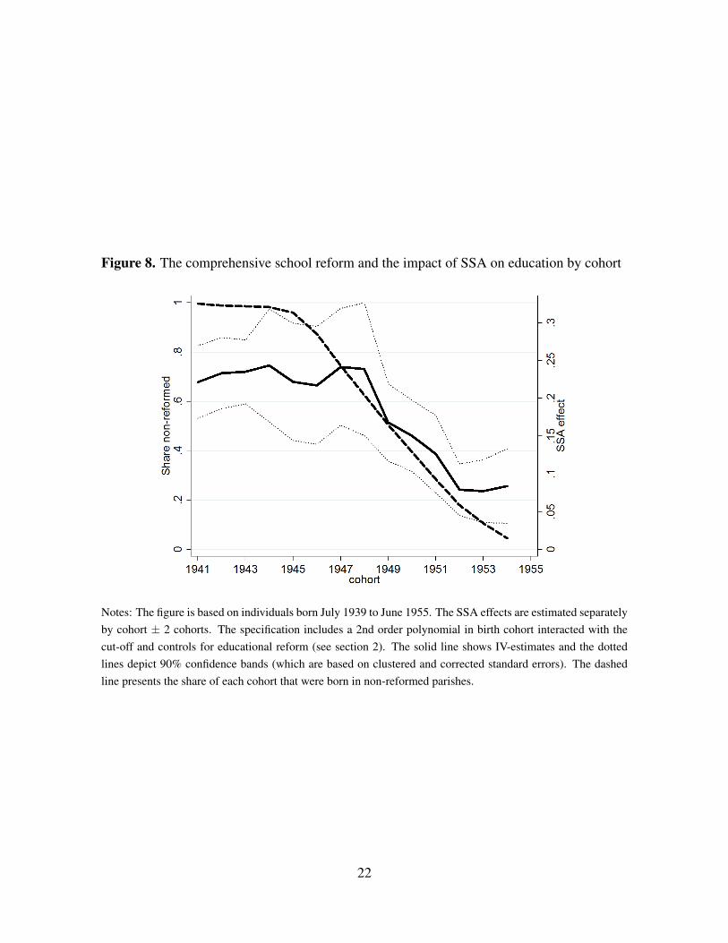
Figure 8. The comprehensive school reform and the impact of SSA on education by cohort

Notes: The figure is based on individuals born July 1939 to June 1955. The SSA effects are estimated separatelyby cohort ± 2 cohorts. The specification includes a 2nd order polynomial in birth cohort interacted with thecut-off and controls for educational reform (see section 2). The solid line shows IV-estimates and the dottedlines depict 90% confidence bands (which are based on clustered and corrected standard errors). The dashedline presents the share of each cohort that were born in non-reformed parishes.

22

where θcR denotes fixed effects that allow the cohort effects to vary by reform and θpR do thesame thing for the parish fixed effects. Notice that the main effect of the reform is swampedby these fixed effects. In equation (6), κ is the coefficient of interest.

An advantage of pooling the regressions is that we can be more flexible in specifying therelationship between birth month and years of schooling than in equation (6). In particularwe can introduce fixed effects for the interaction between cohort and being born after thecut-off as well as fixed effects for cohort by parish. The cohort by parish fixed effects takecare of any trends in educational attainment that vary across parishes (and the main effect ofthe reform). The cohort by cut-off fixed effects take care of any changes in the relationshipbetween education and birth month over cohorts (and the main effect of being born after thecut-off). With the inclusion of these fixed effects, the main effects of the reform and SSA arenot identified, but the coefficient of the interaction term, κ , still is.

Notice that the reform indicator varies by calendar year while our definition of a cohortis from July to June. To ensure that this does not have a mechanical effect on the relationshipbetween being born after the school entry cut-off and educational attainment, we excludethe reform year.14 Moreover, since there is some uncertainty in the timing of the reform wealso exclude the year preceding and following the reform. Notice, finally, that we assignindividuals to reform status on the basis of parish of birth.15

Table 4 shows the results. Since the reform started with individuals born 1942, we excludeindividuals born prior to this year. We also exclude individuals who were born in parishesthat introduced the reform after 1953 since these do not contribute to identification (giventhat we exclude the reform year and the preceding year).16

The first two columns show estimates by reform regime. The reform implies that schoolentry age has a smaller impact on educational attainment as conjectured above. Column (3)shows that the difference between the two estimates is statistically significant and that thedrop in educational attainment amounts to 0.099 years. Column (4) shows the most elaboratespecification which includes fixed effects for cohort by birth month and cohort by parish.Again, SSA has a lower effect on educational attainment in reformed parishes: the estimateon the interaction term is -0.098, with a standard error of 0.046.

14For a reform year, individuals born after the cut-off, who start school at the normal time, automatically getextra schooling relative to those born just before the cut-off.

15The Appendix describes how we assign reform status to individuals.16We could of course include individuals born prior to 1942 in the comparison group. We prefer the current

approach since, a priori, we think the “common trends” assumption is more palatable with fewer years of pre-reform data. Nevertheless, our conclusions do not depend on the sample restriction. With all birth cohorts, theestimate on the interaction term is -0.107 (standard error: 0.037) in a specification corresponding to column (4)in Table 4.

23

Tabl

e4.

The

com

puls

ory

scho

olre

form

and

the

impa

ctof

SSA

oned

ucat

iona

latta

inm

ent

All

By

gend

erB

ypa

rent

aled

R=

1R=

0Fe

mal

esM

ales

Low

Hig

h(1

)(2

)(3

)(4

)(5

)(6

)(7

)(8

)SS

A0.

112*

*0.

212*

*0.

212*

*–

0.24

2**

0.17

6**

0.25

8**

0.19

5**

(0.0

30)

(0.0

42)

(0.0

42)

(0.0

46)

(0.0

59)

(0.0

43)

(0.0

46)

SSA×

refo

rm-0

.099

*-0

.098

**-0

.094

-0.1

00-0

.122

*-0

.096

*(0

.051

)(0

.046

)(0

.057

)(0

.073

)(0

.063

)(0

.058

)C

ohor

tFE

:s√

√

Pari

shFE

:s√

√

Coh

ort×

refo

rmFE

:s√

√√

√√

Pari

sh×

refo

rmFE

:s√

√√

√√

Coh

ort×

(Aft

ercu

t-of

f)FE

:s√

Coh

ort×

pari

shFE

:s√

#in

divi

dual

s35

7,59

865

0,48

71,

008,

085

1,00

8,08

549

0,45

851

7,62

730

7,58

568

1,77

2N

otes

:T

here

gres

sion

sar

eba

sed

onin

divi

dual

sbo

rnaf

ter

1942

who

wer

ebo

rnin

mun

icip

aliti

esth

atin

trod

uced

the

refo

rmpr

ior

to19

54.

All

regr

essi

ons

incl

ude

a2n

dor

derp

olyn

omia

lin

birt

hm

onth

whi

chis

inte

ract

edw

ithth

ecu

t-of

f(it

isno

tide

ntifi

edin

col.

(4)h

owev

er).

The

regr

essi

ons

inco

lum

n(3

)-(8

)in

clud

ea

seco

ndor

der

poly

nom

iali

nbi

rth

mon

thw

hich

isin

tera

cted

with

cut-

off

and

refo

rm.

Indi

vidu

als

with

low

-edu

cate

dpa

rent

sar

ede

fined

asha

ving

mot

hers

and

fath

ers

with

atm

ost7

year

sof

educ

atio

n.St

anda

rder

rors

,sho

wn

inpa

rent

hese

s,al

low

for

clus

teri

ngon

the

disc

rete

valu

esof

the

assi

gnm

ent

vari

able

and

are

corr

ecte

dfo

rthe

two

sam

ple

natu

reof

ourI

Vst

rate

gy;s

eeIn

oue

and

Solo

n(2

010)

.**/

*=

sign

ifica

ntat

the

5/10

perc

entl

evel

.

24

Since the specifications in columns (3) and (4) yield identical results, we proceed with thesimpler specification in column (3). Columns (5)-(8) present separate estimates by gender andparental education. The comprehensive school reform did not affect the relationship betweenSSA and educational attainment differently across groups.

The estimates shown in Table 4 have reduced-form interpretations, since exposure to thereform depends on the parish of residence at the time when the reform was implemented. Tothe extent that individuals change reform status by moving parish, our estimates are lowerbounds on the true treatment effects. Unfortunately we do not have the data do assign aparish of residence to all individuals at age 10 (or age 13). However, the evidence reportedin Meghir and Palme (2005) suggests that the problem is minor. They find that only 9.9%changed reform status by moving. Estimates of the treatment effects can thus be obtained bydividing the reduced form estimates by 0.901 (the fraction that did not change reform status).Interpreted literally, this means that the reform reduced the impact of school starting age oneducational attainment by 0.11 years.

Table 4 shows that initial differences, caused by variation in school starting age, are morelikely to persist in school systems where students are tracked early on. We view this evidenceas substantially more credible than the evidence reported Bedard and Dhuey (2006) whocompared age effects across countries while children are still in school.

8 The effect of SSA on life-time earnings, employment, and wages

The variation in school starting age affects many margins influencing the final earnings out-come. Most obviously, it has an effect on educational attainment. Perhaps as obviously,children who start school one year later enter the labor market one year later, conditional onage and schooling (and thus have less experience throughout the career). In addition, expe-rience is lower because late school starters have more schooling. Finally, their may be otherachievement differences by age at school start conditional on years of compulsory schooling.

This section documents the effects of school starting age on life-time earnings, wages,and employment. Section 8.1 illustrates the effects on the age-earnings profiles. Section 8.2considers the effects on earnings, employment and wages during prime-age. Section 8.3,finally, examines whether the present value of earnings is affected by SSA. Throughout, wefocus on the total effect of school starting age on earnings (without controlling for experienceand schooling). This parameter captures individual benefits and costs of alternative schoolstarting ages.

25

8.1 Effects of school starting age on the age-earnings profile

We present the broad picture in Figure 9. The evidence shown in the figure comes fromestimating equation (1) separately by age using instrumental variables. Earnings at each ageincludes zero-earners and is measured relative to (cohort- and group-specific) mean earningsduring prime-age (age 25-54). The top-left graph shows the effects of SSA on the age-earnings profile, averaged over all individuals. The top-right graph pertains to individualswith low-educated parents; the bottom-left graph to women; and the bottom-right graph tomen.17

Overall, the results are very much in line with the results in Figures 5 and 7. The top-left graph shows the effects of school starting age on the age-earnings profile. On average,there are initial earnings losses due to later labor market entry and consequent loss of experi-ence. But after age 55, until the nominal retirement age, school starting age has positive andsubstantial effects on earnings.18

The positive effects after age 55 are driven by positive employment responses towardsthe end of working life. In other words, school starting age delays retirement. Notice thateligibility for old-age retirement is determined by your birthday. Individuals become eligiblewhen they turn 61. The normal retirement age, prior to the pension reform in the late 1990s,was the 65th birthday. After the pension reform, the statutory retirement age is 67. The focalpoint in retirement behavior is thus the birthday.19

On average, SSA only affects the allocation of labor supply over the life-cycle; there areno effects during prime-age.20 However, the top-right graph shows that the SSA effects aredecidedly more positive for those with low-educated parents than for the remainder of thepopulation. Similarly, the bottom panel illustrates that the effects tend to be more positivefor women than for men.21 As noted earlier, it is for women and individuals with low-educated parents that we find the most positive effect on educational attainment (see Table 3).

17Since individuals with high-educated parents comprise almost three quarters of the sample, the overallshape of the graph for this (omitted) group is similar to the graph for all individuals.

18The exact magnitude of the initial losses and later gains should be interpreted with some care, since wedo not observe all cohorts at all ages. While all cohorts are observed in the age interval 25-55, we primarilyobserve the younger cohorts in the lower age-range and the older cohorts in the upper age-range. Since the SSAeffects on education varies over cohorts, the exact magnitudes at the lower and upper ends of the age-intervalshould be interpreted somewhat carefully. Having said this, we also note that the qualitative nature of the resultsremains for all cohort.

19According to data from LINDA (see Edin and Fredriksson 2000), 75% of individuals born 1915-34 retiredon their birthday.

20Below we show that, on average, there are no wage effects of SSA during prime-age.21The erratic pattern around age 20 for men has to do with military service. Older male school starters enter

the military at an older age. Therefore earnings rebound and then drop around age 20.

26

Figu

re9.

IVes

timat

esof

SSA

onag

e-ea

rnin

gspr

ofile

Not

es:T

heto

p-le

ftgr

aph

show

sSS

Aef

fect

sfo

rall

indi

vidu

als.

The

top-

righ

tgra

phpe

rtai

nsin

divi

dual

sw

ithlo

w-e

duca

ted

pare

nts,

the

botto

m-l

eftg

raph

tow

omen

and

the

botto

m-r

ight

tom

en.

The

regr

essi

ons

are

estim

ated

sepa

rate

lyby

age,

and

alle

stim

ates

are

base

don

coho

rts

born

July

1935

toJu

ne19

55.

Thr

ough

outw

eco

ntro

lfor

coho

rtfix

edef

fect

s,ed

ucat

iona

lref

orm

(see

sect

ion

2),a

nda

2nd

orde

rpo

lyno

mia

lin

birt

hm

onth

whi

chis

inte

ract

edw

ithth

esc

hool

-ent

rycu

t-of

f.E

stim

ates

are

wei

ghte

dto

acco

untf

ora

low

ersa

mpl

ing

prob

abili

tydu

ring

1960

-66.

Tosm

ooth

the

estim

ates

the

depe

nden

tvar

iabl

eis

mea

nea

rnin

gsby

age±

1;th

eA

ppen

dix

expa

nds

onth

ispr

oced

ure.

Das

hed

lines

are

90%

confi

denc

eba

nds

(bas

edon

clus

tere

dan

dco

rrec

ted

stan

dard

erro

rs).

Age

-spe

cific

earn

ings

ism

easu

red

rela

tive

toav

erag

e(c

ohor

t-an

dgr

oup-

spec

ific)

earn

ings

whe

nin

divi

dual

sar

eag

ed25

-54.

27

Individuals with low-educated parents and women are also most likely to be on the extensiveemployment margin.

In comparison to Black et al. (2011) the SSA effects shown in Figure 9 are more sub-stantive. Black et al. (2011) follow individuals when they are aged 24-35. They find initialearnings losses, but by age 30 they have disappeared for both men and women.22 They alsodo a back-of-the envelope calculation assuming that there are no effects beyond age 35. Theyconclude from this exercise that the effects on the present value of life-time earnings is neg-ative. Judging from Figure 9 it is questionable whether this assumption is valid. Overall, wesee no effect at age 35; yet, we observe positive effects of SSA from age 55 until retirement.We return to the effect of SSA on the present value of life-time earnings in Section 8.3.

8.2 Effects of school starting age on earnings, employment and wages during prime-age

This section probes deeper into the effects of school starting age during prime-age. In partic-ular, we examine whether the earnings effects are due to employment or wage responses toschool starting age.

Table 5 reports the results. The different rows display results for various outcomes. Thedifferent columns present results for all (column (1)), as well as by gender (columns (2) and(3)) and by parental education (columns (4) and (5)). Earnings estimates are reported relativeto mean earnings. All estimates are multiplied by 100 to improve readability. Earnings andemployment outcomes are thus reported in terms of percentage points and log wage outcomesin terms of percent.

The first row shows the results for earnings when individuals are prime-aged (25-54).We include years when individuals have no earnings; the estimates are thus not plagued byselection bias and potentially capture both labor supply and wage responses to variations inschool entry age. The second row shows the effects on average employment during prime-age. The remaining two rows show the employment and wage effects when individuals areaged 41-45. We focus on these particular ages since they are in the midst of prime age andsince we lack information on wages prior to 1985. The employment effects are reportedin order to assess whether the wage estimates are plagued by selection bias. If there aresignificant effects on the probability of being full-time employed, the wage effects should beinterpreted with some care.

22It is a bit surprising that the effects in Black et al. (2011) have disappeared by age 30. Figure A1 in theAppendix shows the age premium for men on the Swedish labor market. The wage loss associated with a lossof experience by 1 year is around 2% when individuals are age 32.

28

Table 5. IV estimates of SSA on earnings, employment, and wages

Outcome All By gender By parental ed.(units) Females Males Low High

Age (1) (2) (3) (4) (5)

Earnings 25-54 -0.212 0.992** -0.891** 1.205** -0.719*(ppt.) (0.327) (0.435) (0.386) (0.577) (0.374)

Employment 25-54 0.330** 0.677** -0.039 0.696** 0.232(ppt.) (0.122) (0.178) (0.143) (0.217) (0.148)

Full-time employment 41-45 0.273 0.733** -0.127 0.715** 0.110(ppt.) (0.190) (0.274) (0.182) (0.351) (0.230)

ln(wage) 41-45 -0.274 0.137 -0.810** 0.052 -0.467(percent) (0.253) (0.224) (0.356) (0.334) (0.293)

Notes: To improve readability coefficients and standard error are multiplied by 100. The regressions are basedon individual panel data over the indicated age intervals. The effects of SSA are restricted to be the same acrossages and thus have the interpretation as the average effects over the indicated age intervals. The regressionsinclude individuals born July 1935 to June 1955. Earnings effects are defined relative to the cohort- and group-specific mean. Employment is coded one if annual earnings exceed average earnings for individuals with wagesbelow the 5th percentile. Full-time employment is coded one if annual earnings exceeds minimum full-timeearnings. These earnings cut-offs are defined separately by gender, education, age, and time; see Appendix formore details. ln(wage) is the log of wages. After cutoff (=1 if individuals are born January-June) is used toinstrument SSA. All regressions include cohort fixed effect, a 2nd order polynomial interacted with the cut-off,and control for educational reform (see Section 2). Estimates are weighted to account for a lower samplingprobability during 1960-66. Individuals with low-educated parents are defined as having mothers and fatherswith at most 7 years of education. Standard errors, shown in parentheses, allow for clustering on the discretevalues of the assignment variable and are corrected for the two-sample nature of our IV approach; see Inoueand Solon (2010). **/* = significant at the 5/10 percent level.

29

The first column shows that higher school starting age increases employment duringprime-age by 0.3 percentage points on average. Nevertheless, there is no significant effect onearnings, presumably because forgone experience implies wage losses early on in the career.

Columns (2) and (3) show that the differential effects of SSA on educational attainmentacross gender spill over onto labor market outcomes. For women, we observe a positive effecton employment of 0.8 percentage points and no counteracting wage effect. For men, there isno effect on employment and a negative wage effect of 0.8 percent.

It is a bit surprising to see that the wage effects of starting school a year later persistwhen individuals are aged 41-45. The initial loss of experience seems to have very persistenteffects. In fact, the negative wage impact for men does not disappear until individuals areaged 50. Figure A1 in the Appendix, which shows the age premium for men, corroboratesthis finding. The age premium for men is 1% when individuals are aged 43; it stays positiveuntil individuals are 55 years-of-age. It is not until age 55 that the initial loss of experienceis irrelevant.

A related question is whether the increase in educational attainment (in response to higherSSA) leaves a traceable impact on wages. In comparison to the U.S., returns to skills inSweden are low. OLS estimates of the returns to education typically hover around 4 to 5percent; see Leuven et al. (2004) for instance. When the increase in educational attainmentis only relevant, this suggests a wage impact for men in the order of 0.5%. At the returnsto education typically found on the Swedish labor market, it will thus be hard to detect aneffect of SSA on wages. In our view, it is more likely that the effects can be found along theextensive margin for groups that tend to be marginal.

Columns (4) and (5) present separate estimates with respect to parental education. Indi-viduals whose parents are low-educated seem to gain from starting school at an older age,while the opposite is true for individuals with well-educated parents. Again, the differentialeffects on educational attainment map onto labor market outcomes; see Table 3. Moreover,the increase in education primarily leads to a response along the extensive margin for individ-uals with less educated parents. For this group of individuals, an increase in school startingage by 1 year raises average employment by 0.7 percentage points.

The overall message delivered by Table 5 is that school starting age has positive effectson the extensive margin for groups that tend to be marginal. For core workers, there is noemployment response and sometimes a negative wage impact stemming from the initial lossof experience. Consistent with this, Figure 9 shows that we find positive effects close toretirement, i.e., at a point in the life-cycle where labor supply is highly elastic for all workers.

The regression results in Table 5 pools together all cohorts. Over cohorts (time), the

30

female participation rate increased substantially. Table A1 shows that the employment rateof females aged 30-34 increased from 54% in the cohorts born 1935-45 to 81% in the cohortsborn 1945-55. This increase is most likely tied to a series of reforms implemented in the1960s and 1970s. For instance, there was a move from household to individual taxation,child-care was built up, and a parental leave system was introduced. Females in the youngercohorts should arguably be considered core workers.

Now if females, to some extent, moved from being marginal to core workers and if schoolstarting age primarily operates along the extensive employment margin, we should expectsmaller effects of SSA on prime-age earnings over cohorts. Auxiliary regressions (not shown)suggest a decline in the effect of SSA on prime-age earnings for females over cohorts. Wedo not observe a corresponding decline for individuals with low-educated parents, a groupthat is likely to have been marginal throughout the time-period spanned by these data. Thissuggests that labor market attachment is also important for the effect of SSA on prime-ageearnings.

8.3 Effects of school starting age on present value of earnings

The gains and losses of school starting age occur at various stages of the life-cycle (see Figure9). The natural way of trading off initial losses with subsequent gains is to estimate the effecton the present value of earnings. This is the purpose of this section.

To conduct the analysis we must handle the fact that all cohorts are not observed through-out their careers. For the oldest cohorts, we miss the young ages and thus underrepresent thecost of entering school later; for the younger cohort, we miss the ages close to retirement and,therefore, the gains of starting later. We deal with this problem by placing additional weighton the cohorts observed during the ages that are missing for some cohorts.

The results from this exercise should be interpreted a bit carefully since Figure 8 showsthat the effects of SSA vary somewhat across cohorts. Note, though, that we have also usedonly the cohorts that we we observe throughout the labor market career (those born July 1943to June 1945) and do not get appreciably different results.

Table 6 reports the results. We take the entire earnings stream from age 18 to 64 intoaccount and discount to present value at age 18. Across rows we present the results foralternative discount rates. The estimates are multiplied by 100 and reported relative to thepresent value of cohort-specific prime-age earnings.

The first row of Table 6 summarizes Figure 9. There is no effect on average. The pos-itive effects for women and individuals with low-educated parents during prime-age are not

31

Table 6. Effect of SSA on present value of earnings

All By gender By parental edFemales Males Low High

Discount rate (1) (2) (3) (4) (5)

r = 0.00 -0.513 0.614 -1.197** 0.720 -0.941**(0.380) (0.535) (0.438) (0.647) (0.413)

r = 0.02 -0.864** 0.163 -1.480** 0.219 -1.240**(0.343) (0.496) (0.381) (0.586) (0.372)

r = 0.05 -1.440** -0.572 -1.955** -0.610 -1.725**(0.359) (0.525) (0.386) (0.600) (0.391)

Notes: Estimates are multiplied by 100 to improve readability. The regressions are based on individuals bornJuly 1935 to June 1955. The present values are normalized by the cohort-specific discounted value of prime-ageearnings. All regressions include cohort fixed effect, control for educational reform (see section 2), as well as asecond order polynomial in birth month which is interacted with cut-off. After cutoff (=1 if individuals are bornJanuary-June) is used to instrument SSA. Estimates are weighted to account for a lower sampling probabilityduring 1960-66. Moreover, we weight the data to account for the fact that some cohorts are not observed duringall ages. Individuals with low-educated parents are defined as having mothers and fathers with at most 7 years ofeducation. Standard errors, shown in parentheses, are clustered on the discrete values of the assignment variableand corrected for the two-sample nature of our IV approach; see Inoue and Solon (2010). **/* = significant atthe 5/10 percent level.

32

sufficiently large to render the estimates statistically significant. For men and those withhigh-educated parents, there are (statistically) significant losses amounting to 1.2 and 0.9percentage points respectively.

The second row shows the results when we discount the earnings stream at a realistic rate(2%). The effect of SSA on discounted life-time earnings is -0.9% of prime-age earnings forthe average workers. With heavier discounting (5%) we get uniformly lower estimates; seethird row.

According to Table 6, there is no group where school entry age has a significant increasein discounted life-time earnings. Initial losses outweigh subsequent gains. With realistic dis-count rates, the loss amounts to 0.9 percent of discounted prime-age earnings for the averageworker.

9 Conclusion

We study the long-run impact of school starting age among the cohorts born 1935-55. Higherschool starting age implies an initial advantage which increases educational attainment inthe long run. On average, an increase in school starting age by one year raises educationalattainment by 0.16 years. The effects on educational attainment are more substantive than theeffects found in a comparable study for Norway (see Black et al. 2011).

We show that the comprehensive school reform (which postponed tracking until age 16)reduced the effect of school starting age on educational attainment. Postponing tracking toan older age thus reduces the importance of having an initial advantage. This is the first paperthat documents such effects in a convincing fashion.

A further value added of our study is that we trace the effects of entry age on prime-ageearnings, employment, and wages for any given cohort. Overall, school starting age onlyaffects the allocation of labor supply over the life-cycle. There are initial losses due to laterentry into the labor market, but also later gains since those who start at an older age retire later.For individuals with low-educated parents, and to some extent women, we find increases inprime-age earnings in response to school starting age. Our favored interpretation is that therise in educational attainment, caused by school starting age, primarily affects individualswho are likely to be on the extensive margin.

The impact of school entry age on employment and earnings around retirement impliesthat studies which do not observe outcomes throughout the career are potentially misleadingin terms of the life-time earnings impact. Despite higher earnings around retirement, how-ever, there is no group where we find that school starting age causes statistically significant

33

increases in discounted life-time earnings. On average, discounted life-time earnings fall by0.9 percent (relative to discounted prime-age earnings) in response to later school start (at adiscount rate of 2%).

In summary, we think there are two general lessons from our analysis. First, our evidenceshows that initial advantages are exacerbated by early tracking. Countries wishing to reducethe importance of initial advantage may consider postponing tracking. Second, any labormarket effects of school starting age likely operate along the extensive employment marginand are, therefore, more important for marginal groups. In our view, it is unlikely that schoolstarting age leaves traceable wage impacts for core groups on the labor market.

34

References

Angrist, J.D. and Krueger, A.B. (1991). ‘Does compulsory school attendance affect schoolingand earnings?’, Quarterly Journal of Economics, vol. 106, pp. 979–1014.

Angrist, J.D. and Krueger, A.B. (1992). ‘The effect of age at school entry on educationalattainment: An application of instrumental variables with moments from two samples’,Journal of the American Statistical Association, vol. 87, pp. 328–336.

Angrist, J.D. and Pischke, J.S. (2008). Mostly Harmless Econometrics, Princeton UniversityPress.

Bedard, K. and Dhuey, E. (2006). ‘The persistence of early childhood maturity: Internationalevidence of long-run age effects’, Quarterly Journal of Economics, vol. 121, pp. 1437–1472.

Black, S.E., Devereux, P.J. and Salvanes, K.G. (2011). ‘Too young to leave the nest? theeffects of school starting age’, Review of Economics and Statistics, vol. 93, pp. 455–467.

Datar, A. (2006). ‘Does delaying kindergarten entrance give children a head start?’, Eco-

nomics of Education Review, vol. 25, pp. 43–62.

Dobkin, C. and Ferreira, F. (2010). ‘Do school entry laws affect educational attainment andlabor market outcomes?’, Economics of Education Review, vol. 29, pp. 40–54.

Edin, P.A. and Fredriksson, P. (2000). ‘Linda – longitudinal individual data for sweden’,Department of Economics, Uppsala University.

Elder, T.E. and Lubotsky, D.H. (2009). ‘Kindergarten entrance age and children’s achieve-ment: Impacts of state policies, family background, and peers’, Journal of Human Re-

sources, vol. 44, pp. 641–683.

Fertig, M. and Kluve, J. (2005). ‘The effect of age at school entry on educational attainmentin germany’, IZA.

Fredriksson, P. and Öckert, B. (2005). ‘Is early learning really more productive? the effect ofthe school starting age on school and labor market performance’, IZA.

Holmlund, H. (2007). ‘A researchers guide to the swedish compulsory school reform’, SOFI,Stockholm University.

35

Härnquist, K. (2000). ‘Evaluation through follow-up’, in (C. Jansson, ed.), Seven Swedish

Longitudinal Studies in the Behavioral Sciences, Forskningsrådsnämnden, Stockholm.

Inoue, A. and Solon, G. (2010). ‘Two-sample instrumental variables estimators’, Review of

Economics and Statistics, vol. 92, pp. 557–561.

Lee, D.S. and Card, D. (2008). ‘Regression discontinuity inference with specification error’,Journal of Econometrics, vol. 142, pp. 655–674.

Leuven, E., Oosterbeek, H. and van Ophem, H. (2004). ‘Explaining international differencesin male wage inequality by differences in demand and supply of skill’, Economic Journal,vol. 144, pp. 478–498.

McCrary, J. (2008). ‘Manipulation of the running variable in the regression discontinuitydesign: A density test’, Journal of Econometrics, vol. 142, pp. 698–714.

Meghir, C. and Palme, M. (2005). ‘Educational reform, ability and parental background’,American Economic Review, vol. 95, pp. 414–424.

Muhlenweg, A.M. and Puhani, P.A. (2010). ‘The evolution of the school-entry age effect ina school tracking system’, Journal of Human Resources, vol. 45(2), pp. 407–438.

Murphy, K.M. and Topel, R.H. (1985). ‘Estimation and inference in two-step econometricmodels’, Journal of Business and Economic Statistics, vol. 3, pp. 370–379.

Plug, E. (2001). ‘Season of birth, schooling and earnings’, Journal of Economic Psychology,vol. 22, pp. 641–660.

J. P. Shonkoff and D. A. Phillips, eds. (2000). From Neurons to Neighborhoods: The Science

of Early Childhood Development, National Academy Press.

Stipek, D. (2002). ‘At what age should children enter kindergarten? a question for policymakers and parents’, Social Policy Report, vol. 16, pp. 3–16.

36

AppendixDescriptive statistics

Earnings and employment Table A1 reports descriptive statistics on earnings, full-time em-ployment, and employment by cohort, gender, parental education, and age.

Age premium for men Figure A1 shows non-parametric estimates of the age-wage premiumfor men. The estimates are derived by comparing the log wages of two adjacent cohorts foreach age while holding time constant. When individuals are 43 years-of-age, there is a onepercent effect of age on wages. After 54 years-of-age, the age premium turns negative.

Figure A1: Age premium for men, 1935-55 cohorts

Notes: The graph on the left shows estimates of the age premium. The graph on the right cumulates theseestimates using the mean log wage at age 31 as the starting point. The estimates are based on wage dataavailable from 1985-2009, and the cohorts born July 1935 to June 1955. Identification of the full age range is tosome extent achieved by pooling cohorts. For someone born 1935 we observe wages from age 50 and onwards.For someone born 1955 we observe wages from age 30 to 54. Estimates are obtained by comparing to adjacentcohorts by age while holding time constant (time fixed effects). Dashed lines are 90% confidence bands (basedon clustered standard errors).

37

Tabl

eA

1:M

eans

ofea

rnin

gsan

dem

ploy

men

tC

ohor

tsbo

rn19

35-4

5C

ohor

tsbo

rn19

45-5

5A

llG

ende

rPa

rent

aled

.A

llG

ende

rPa

rent

aled

.M

ales

Fem

ales

Low

Hig

hM

ales

Fem

ales

Low

Hig

hA

ge(1

)(2

)(3

)(4

)(5

)(6

)(7

)(8

)(9

)(1

0)E

arni

ngs

20-2

40.

425

0.42

00.

433

0.47

50.

409

0.45

90.

443

0.48

40.

526

0.42

6(0

.333

)(0

.272

)(0

.372

)(0

.328

)(0

.331

)(0

.317

)(0

.277

)(0

.354

)(0

.322

)(0

.313

)30

-34

0.88

00.

968

0.67

60.

872

0.88

10.

852

0.89

40.

782

0.86

10.

848

(0.6

76)

(0.4

58)

(0.6

84)

(0.6

16)

(0.6

85)

(0.4

75)

(0.3

66)

(0.4

85)

(0.4

61)

(0.4

79)

40-4

41.

101

1.07

51.

161

1.09

41.

101

1.05

01.

040

1.06

71.

044

1.05

2(0

.706

)(0

.574

)(0

.702

)(0

.620

)(0

.718

)(0

.631

)(0

.591

)(0

.566

)(0

.570

)(0

.653

)50

-54

1.18

51.

089

1.39

41.

169

1.18

61.

275

1.22

81.

354

1.24

81.

288

(0.8

01)

(0.7

12)

(0.8

10)

(0.7

41)

(0.8

08)

(0.9

44)

(0.9

32)

(0.8

33)

(0.8

24)

(0.9

87)

60-6

40.

930

0.84

81.

113

0.93

70.

928

1.18

61.

121

1.30

31.

160

1.19

7(1

.006

)(0

.934

)(1

.042

)(0

.890

)(1

.025

)(1

.070

)(1

.020

)(1

.042

)(0

.966

)(1

.106

)Fu

ll-tim

eem

ploy

men

t20

-24

0.24

60.

408

0.07

50.

267

0.23

90.

369

0.49

50.

236

0.41

00.

345

(0.3

44)

(0.3

75)

(0.1

95)

(0.3

54)

(0.3

40)

(0.3

88)

(0.3

91)

(0.3

37)

(0.3

95)

(0.3

82)

30-3

40.

596

0.88

00.

290

0.57

70.

604

0.71

30.

923

0.49

40.

685

0.72

8(0

.439

)(0

.232

)(0

.401

)(0

.440

)(0

.438

)(0

.404

)(0

.214

)(0

.438

)(0

.415

)(0

.397

)40

-44

0.76

70.

940

0.58

80.

762

0.77

10.

825

0.90

20.

746

0.81

80.

830

(0.3

92)

(0.2

12)

(0.4

50)

(0.3

94)

(0.3

90)

(0.3

42)

(0.2

61)

(0.3

94)

(0.3

47)

(0.3

39)

50-5

40.

753

0.86

90.

634

0.73

50.

759

0.80

60.

859

0.75

10.

800

0.81

0(0

.402

)(0

.304

)(0

.451

)(0

.410

)(0

.398

)(0

.369

)(0

.320

)(0

.405

)(0

.373

)(0

.366

)60

-64

0.56

40.

657

0.47

10.

559

0.56

70.

684

0.75

50.

612

0.67

10.

691

(0.4

56)

(0.4

33)

(0.4

60)

(0.4

57)

(0.4

56)

(0.4

33)

(0.3

96)

(0.4

56)

(0.4

38)

(0.4

30)

Em

ploy

men

t20

-24

0.69

00.

788

0.58

50.

727

0.67

80.

718

0.77

70.

656

0.76

80.

691

(0.3

74)

(0.3

20)

(0.3

98)

(0.3

60)

(0.3

78)

(0.3

59)

(0.3

32)

(0.3

75)

(0.3

35)

(0.3

68)

30-3

40.

720

0.88

90.

538

0.71

60.

724

0.87

20.

935

0.80

70.

861

0.87

9(0

.382

)(0

.221

)(0

.432

)(0

.380

)(0

.382

)(0

.286

)(0

.198

)(0

.344

)(0

.294

)(0

.281

)40

-44

0.90

00.

943

0.85

60.

906

0.90

10.

896

0.90

40.

888

0.90

10.

894

(0.2

69)

(0.2

07)

(0.3

15)

(0.2

60)

(0.2

68)

(0.2

71)

(0.2

58)

(0.2

83)

(0.2

63)

(0.2

74)

50-5

40.

870

0.88

90.

852

0.86

50.

873

0.86

40.

874

0.85

50.

868

0.86

3(0

.308

)(0

.282

)(0

.331

)(0

.312

)(0

.305

)(0

.319

)(0

.306

)(0

.330

)(0

.314

)(0

.321

)60

-64

0.68

30.

703

0.66

30.

684

0.68

50.

770

0.78

90.

750

0.76

70.

772

(0.4

27)

(0.4

16)

(0.4

36)

(0.4

26)

(0.4

26)

(0.3

93)

(0.3

77)

(0.4

08)

(0.3

95)

(0.3

91)

Not

es:T

hesa

mpl

ein

cols

(1)-

(5)i

nclu

des

indi

vidu

als

born

July

1935

toJu

ne19

45an

dth

esa

mpl

ein

cols

(6)-

(10)

indi

vidu

als

born

July

1945

toJu

ne19

55.

Ear

ning

sis

defin

edre

lativ

eto

the

coho

rt-s

peci

ficm

ean

whe

nin

divi

dual

sar

eag

ed25

-55.

Full-

time

empl

oym

enti

sco

ded

one

ifan

nual

earn

ings

exce

eds

min

imum

full-

time

earn

ings

;se

eA

ppen

dix

for

mor

ede

tails

.D

etai

lson

the

cons

truc

tion

ofth

eem

ploy

men

tind

icat

orar

eal

soav

aila

ble

inth

eA

ppen

dix.

Num

bers

repo

rted

inth

eta

ble

are

aver

ages

over

the

indi

cate

dag

es.S

tand

ard

devi

atio

nsin

pare

nthe

ses.

38

Construction of key variables

Employment indicators We construct the employment indicators by the mapping from thecross-sectional distribution of wages and earnings in 2009. We divide the data into “cells”on the basis of gender (2 categories), education (5 categories), and age (9 categories); thecombination of these categories yield 90 cells. For each cell, we calculate a “minimumwage”, i.e. the wage on the 1st percentile, and a “low wage”, the wage at the 5th percentile.Wages are reported as monthly full-time equivalent wages.

To construct the full-time employment indicator we take the minimum wage times 12to correspond to minimum annual earnings. Then, for each cell, we calculate the earningspercentile corresponding to this minimum annual earnings threshold. Finally, for each year ofobservation and each cell, we define everyone earning above the minimum earnings percentileas full-time employed.

To construct the employment indicator, we calculate average earnings for everyone withwages below the 5th percentile. Then, for each cell, we calculate the earnings percentilecorresponding to this annual employment threshold. Finally, for each year of observation andeach cell, we define everyone earning above this threshold percentile as employed.

Age-specific earnings Earnings data are available for 1960-66, 1968, 1970-71, 1973, 1975-76, 1979-80, 1982, 1985-2009. Take someone born in 1940 for instance. For this individual,earnings are observed at age 20-26, 28, 30-31, 33, 35-36, 39-40, 42, and 45-69. For anindividual born 1945, earnings are available at age 16-21, 23, 25-26, 28, 30-31, 34-35, 37,40-64. This implies that the amount of earnings information varies somewhat over cohortsand that the earnings data do not represent the true relative size of cohorts at a given age.Since there are cohort effects (see Figure 8), we would like the earnings data to represent therelative size of cohorts in the population.

In general we calculate age-specific earnings as a moving average of earnings for a partic-ular age ±1. For an age where there is no information, we use the preceding and subsequentage to fill in the blank. We only fill in blanks if there is information for a preceding andsubsequent year. In a few instances we use information that is more distant than age ±1. Forexample, an individual born in 1940 has no earnings information at age 37. For this individ-ual we calculate earnings at age 37 as a weighted average of earnings at age 36 and earningsat age 39, where earnings at age 39 receive lower weight since it is more distant than earningsat age 36. Using this approach we obtain earnings data for each age between the ages 21-68for the individual born 1940 and between the age 17-63 for the individual born 1945.

39

This approach smooths the estimates somewhat and ensures that each cohort gets theweight it should have if earnings information was available for the entire 1960-2009 period.Notice, however, that we do not (artificially) improve the precision of the estimates (sincestandard errors are clustered on the discrete values of the assignment variable). Also, theeffects on the age-earnings profile have a very similar flavor if we treat the data as a standardunbalanced panel.

Assigning reform status We follow Holmlund (2007) in assigning reform status to individ-uals. The principal input into this calculation is the population census from 1970. In thecensus we whether individuals have 7, 8, 9, or more than 9 years of education. We dropeveryone with more than 9 years of schooling. Now, 7 years of schooling correspond to oldcompulsory school, 8 years of schooling correspond to “extended compulsory school”, and 9years of schooling to the comprehensive school. We define two dummy variables associatedwith 8 and 9 years of schooling and then collapse the data by birth parish and year of birth.Whenever the mean of any of these two dummy variables exceed 0.5, we code the parish ashaving implemented the reform in question from this point and onwards.

Cohort weighting in the analysis the present value of earnings

Because of the availability of earnings data, all cohorts are not observed throughout theircareers. For the oldest cohorts, we miss the young ages and thus underrepresent the costof entering school later; for the younger cohort, we miss the ages close to retirement and,therefore, the gains of starting later. To deal with this problem we place additional weight onthe cohorts observed during the ages that are missing for some cohorts.

To be concrete, consider earnings at age 18. Earnings at age 18 is observed starting withthe 1943 cohort.23 Therefore, we observe earnings at this age for 12 of the 20 cohorts. Toadequately represent earnings at age 18 in the present value calculation, we place the weight20/12 on earnings observations at age 18. Analogously, earnings at age 19 is available startingwith the 1942 cohort, and thus observed for 13 of the 20 cohorts. Earnings observations atage 19 thus receive the weight 20/13. At the other end of the age spectrum, earnings at age 55is unobserved for 1 cohort (the 1954 cohort). Earnings observations at age 55 thus receive theweight 20/19. In general we weight earnings at a particular age with #cohorts/(#non-missingcohorts at that age).

23Remember that we construct age-specific earnings by averaging earnings over three ages (age±1). There-fore we loose the first and the last observation for each cohort.

40

Figure A2. Number of births (left) and parental education (right) by day of birth (5, 15, 25)

Note: The graph on the left shows the distribution of births by birthday (5, 15, 25) among native men who areborn between July 1935 and June 1940. The graph on the right shows parental years of schooling by birthday(5, 15, 25) for the same population. Parental education is defined as the maximum of the education of the fatherand the mother. Discontinuity at cut-off (left): 0.00013 (standard error: 0.00081). Discontinuity at cut-off(right): 0.0298 (standard error: 0.0631). The solid vertical line depicts the school-entry cut-off. Regressionlines are 2nd order polynomials fitted separately to the data on both sides of the cut-off. Throughout we controlfor cohort. In the figure on the right we control for educational reform (see section 2) as well. Controlling foreducational reform is not necessary (without the controls the discontinuity estimate is 0.0137 (standard error:0.0579)) but consistent with our baseline specification.

Further evidence on the validity of the RD-design

Our main data only contains information on birth month. However, the earnings data during1960-66 include information on birthday for those born on the 5th, 15th, or the 25th. Indi-viduals are included in the earnings data if they have ever worked during 1960-66. For menborn between July 1935 and June 1940, 99.2-99.7% of the target population are included inthe earnings data. For men in later cohorts and women, coverage is substantially lower. Here,we present additional evidence on the validity of the RD-design using these data focusing onmen born 1935-40. Since gender is random, the focus on men should be inconsequential.

Figure A2 presents the evidence. The left-hand panel (number of births) is analogousto Figure 1 and the right-hand panel (parental schooling) is analogous to Figure 2. Bothpanels show that there is no shift around the discontinuity when we use the more detailedinformation on day of birth. We have also run the McCrary (2008) test on the data shown tothe left. The estimated shift in the log of the density is 0.0108 with a standard error of 0.0451(the estimate was obtained using a bandwidth of 1 and a smoothing parameter of 3).

41