lidar and camera detection fusion in a real-time
TRANSCRIPT

Article
LiDAR and Camera Detection Fusion in a Real-TimeIndustrial Multi-Sensor Collision Avoidance System
Pan Wei * ID , Lucas Cagle, Tasmia Reza, John Ball ID and James Gafford
Center for Advanced Vehicular Systems (CAVS), Mississippi State University, Mississippi State, MS 39759, USA;[email protected] (L.C.); [email protected] (T.R.); [email protected] (J.B.); [email protected] (J.G.)* Correspondence: [email protected]; Tel.: +1-662-312-1916
Received: 14 May 2018; Accepted: 26 May 2018; Published: 30 May 2018�����������������
Abstract: Collision avoidance is a critical task in many applications, such as ADAS (advanceddriver-assistance systems), industrial automation and robotics. In an industrial automationsetting, certain areas should be off limits to an automated vehicle for protection of people andhigh-valued assets. These areas can be quarantined by mapping (e.g., GPS) or via beacons thatdelineate a no-entry area. We propose a delineation method where the industrial vehicle utilizesa LiDAR (Light Detection and Ranging) and a single color camera to detect passive beacons andmodel-predictive control to stop the vehicle from entering a restricted space. The beacons are standardorange traffic cones with a highly reflective vertical pole attached. The LiDAR can readily detect thesebeacons, but suffers from false positives due to other reflective surfaces such as worker safety vests.Herein, we put forth a method for reducing false positive detection from the LiDAR by projecting thebeacons in the camera imagery via a deep learning method and validating the detection using a neuralnetwork-learned projection from the camera to the LiDAR space. Experimental data collected atMississippi State University’s Center for Advanced Vehicular Systems (CAVS) shows the effectivenessof the proposed system in keeping the true detection while mitigating false positives.
Keywords: multi-sensor; fusion; deep learning; LiDAR; camera; ADAS
1. Introduction
Collision avoidance systems are important for protecting people’s lives and preventingproperty damage. Herein, we present a real-time industrial collision avoidance sensor system, which isdesigned to not run into obstacles or people and to protect high-valued equipment. The system utilizesa scanning LiDAR and a single RGB camera. A passive beacon is utilized to mark off quarantinedareas where the industrial vehicle is not allowed to enter, thus preventing collisions with high-valuedequipment. A front-guard processing mode prevents collisions with objects directly in front ofthe vehicle.
To provide a robust system, we utilize a Quanergy eight-beam LiDAR and a single RGB camera.The LiDAR is an active sensor, which can work regardless of the natural illumination. It can accuratelylocalize objects via their 3D reflections. However, the LiDAR is monochromatic and cannot differentiateobjects based on color. Furthermore, for objects that are far away, the LiDAR may only have one totwo beams intersecting the object, making reliable detection problematic. Unlike LiDAR, RGB camerascan make detection decisions based on texture, shape and color. An RGB stereo camera can be used todetect objects and to estimate 3D positions. However, stereo cameras require extensive processing andoften have difficulty estimating depth when objects lack textural cues. On the other hand, a single RGBcamera can be used to accurately localize objects in the image itself (e.g., determine bounding boxesand classify objects). However, the resulting localization projected into 3D space is poor compared tothe LiDAR. Furthermore, the camera will degrade in foggy or rainy environments, whereas the LiDAR
Electronics 2018, 7, 84; doi:10.3390/electronics7060084 www.mdpi.com/journal/electronics
Electronics 2018, 7, 84 2 of 32
can still operate effectively. Herein, we utilize both the LiDAR and the RGB camera to accurately detect(e.g., identify) and localize objects. The focus of this paper is the fusion method, and we also highlightthe LiDAR detection since it is not as straightforward as the camera-based detection. The contributionsof this paper are:
• We propose a fast and efficient method that learns the projection from the camera space to theLiDAR space and provides camera outputs in the form of LiDAR detection (distance and angle).
• We propose a multi-sensor detection system that fuses both the camera and LiDAR detections toobtain more accurate and robust beacon detections.
• The proposed solution has been implemented using a single Jetson TX2 board (dual CPUs anda GPU) board to run the sensor processing and a second TX2 for the model predictive control(MPC) system. The sensor processing runs in real time (5 Hz).
• The proposed fusion system has been built, integrated and tested using static and dynamicscenarios in a relevant environment. Experimental results are presented to show the fusion efficacy.
This paper is organized as follows: Section 2 introduces LiDAR detection, camera detectionand the fusion of LiDAR and camera. Section 3 discusses the proposed fusion system, and Section 4gives an experimental example showing how fusion and the system work. In Section 5, we comparethe results with and without fusion. Finally, Section 6 contains conclusions and future work.
2. Background
2.1. Camera Detection
Object detection from camera imagery involves both classification and localization of each objectin which we have interest. We do not know ahead of time how many objects we expect to find in eachimage, which means that there is a varying number of outputs for every input image. We also do notknow where these objects may appear in the image, or what their sizes might be. As a result, the objectdetection problem becomes quite challenging.
With the rise of deep learning (DL), object detection methods using DL [1–6] have surpassedmany traditional methods [7,8] in both accuracy and speed. Based on the DL detection methods,there are also systems [9–11] improving the detection results in a computationally-intelligent way.Broadly speaking, there are two approaches for image object detection using DL. One approach isbased on region proposals. Faster R-CNN [3] is one example. This method first runs the entire inputimage through some convolutional layers to obtain a feature map. Then, there is a separate regionproposal network, which uses these convolutional features to propose possible regions for detection.Last, the rest of the network gives classification to these proposed regions. As there are two parts in thenetwork, one for predicting the bounding box and the other for classification, this kind of architecturemay significantly slow down the processing speed. Another type of approach uses one network forboth predicting potential regions and for label classification. One example is you only look once(YOLO) [1,2]. Given an input image, YOLO first divides the image into coarse grids. For each grid,there is a set of base bounding boxes. For each base bounding box, YOLO predicts offsets off thetrue location, a confidence score and classification scores if it thinks that there is an object in that gridlocation. YOLO is fast, but sometimes can fail to detect small objects in the image.
2.2. LiDAR Detection
For LiDAR detection, the difficult part is classifying points based only on a sparse 3D point cloud.One approach [12] uses eigen-feature analysis of weighted covariance matrices with a support vectormachine (SVM) classifier. However, this method is targeted at dense airborne LiDAR point clouds.In another method [13], the feature vectors are classified for each candidate object with respect toa training set of manually-labeled object locations. With its rising popularity, DL has also been used for3D object classification. Most DL-based 3D object classification problems involve two steps: deciding
Electronics 2018, 7, 84 3 of 32
a data representation to be used for the 3D object and training a convolutional neural network (CNN)on that representation of the object. VoxNet [14] is a 3D CNN architecture for efficient and accurateobject detection from LiDAR and RGBD point clouds. An example of DL for volumetric shapes is thePrinceton ModelNet dataset [15], which has proposed a volumetric representation of the 3D model anda 3D volumetric CNN for classification. However, these solutions also depend on a high density (highbeam count) LiDAR, so they would not be suitable for a system with an eight-beam Quanergy M8.
2.3. Camera and LiDAR Detection Fusion
Different sensors for object detection have their advantages and disadvantages. Sensor fusionintegrates different sensors for more accurate and robust detection. For instance, in object detection,cameras can provide rich texture-based and color-based information, which LiDAR generally lacks.On the other hand, LiDAR can work in low visibility, such as at night or in moderate fog or rain.Furthermore, for the detection of the object position relative to the sensor, the LiDAR can providea much more accurate spatial coordinate estimation compared to a camera. As both camera and LiDARhave their advantages and disadvantages, when fusing them together, the ideal algorithm should fullyutilize their advantages and eliminate their disadvantages.
One approach for camera and LiDAR fusion uses extrinsic calibration. Some works on thisapproach [16–18] use various checkerboard patterns or look for corresponding points or edges in boththe LiDAR and camera imagery. Other works on this approach [19–23] look for corresponding points oredges in both the LiDAR and camera imagery in order to perform extrinsic calibration. However, for themajority of works on this approach, the LiDARs they use have either 32 or 64 beams, which providerelatively high vertical spatial resolution, but are prohibitively expensive. Another example is [24],which estimates transformation matrices between the LiDAR and the camera. Other similar examplesinclude [25,26]. However, these works are only suitable for modeling of indoor and short-rangeenvironments. Another approach uses a similarity measure. One example is [27], which automaticallyregisters LiDAR and optical images. This approach also uses dense LiDAR measurements. A thirdkind of approach uses stereo cameras and LiDAR for fusion. One example is [28], which fuses sparse3D LiDAR and dense stereo image point clouds. However, the matching of corresponding points instereo images is computationally complex and may not work well if there is little texture in the images.Both of these approaches require dense point clouds and would not be effective with the smallerLiDARs such as the Quanergy M8. Comparing with previous approaches, the proposed approach inthis paper is unique in two aspects: (1) a single camera and relatively inexpensive eight-beam LiDARare used for an outdoor collision avoidance system; and (2) the proposed system is a real-time system.
2.4. Fuzzy Logic
When Zadeh invented the term “fuzzy” to describe the ambiguities in the world, he developeda language to describe his ideas. One of the important terms in the “fuzzy” approach is the fuzzy set,which is defined as a class of objects with a continuum of grades of membership [29]. The relationbetween a linguistic variable and the fuzzy set is described as “a linguistic variable can be interpretedusing fuzzy sets” in [30]. This statement basically means a fuzzy set is the mathematical representationof linguistic variables. An example of a fuzzy set is “a class of tall students”. It is often denoted asA∼ or sometimes A. The membership function assigns to each object a grade of membership ranging
between zero and one [29].Fuzzy logic is also proposed in [29] by Zadeh. Instead of giving either true or false conclusions,
fuzzy logic uses degrees of truth. The process of fuzzy logic includes three steps. First, input is fuzzifiedinto the fuzzy membership function. Then, IF-THEN rules are applied to produce the fuzzy outputfunction. Last, the fuzzy output function is de-fuzzified to get specific output values. Thus, fuzzy logiccan be used to reason with inputs that have uncertainty.
Zhao et al. [31] applied fuzzy logic to fuse Velodyne 64-beam LiDAR and camera data.They utilized LiDAR processing to classify objects and then fused the classifications based on the

Electronics 2018, 7, 84 4 of 32
bounding box size (tiny, small, middle or large), the image classification result, the spatial and temporalcontext of the bounding box and the LiDAR height. Their system classified outputs as greenery, middleor obstacle. Again, the use of a Velodyne 64-beam LiDAR is prohibitively expensive for our application.
Fuzzy logic provides a mathematically well-founded mechanism for fusion with semanticmeaning, such as “the LiDAR detects an object with high confidence”. This semantic statementcan be quantified mathematically by the fuzzy function. The fuzzy logic system can then be usedto fuse the fuzzified inputs, using the rules of fuzzy logic. Herein, we apply fuzzy logic to combineconfidence scores from the camera and the LiDAR to obtain a detection score for the final fusion result.
3. Proposed System
3.1. Overview
The proposed system architecture block diagram is shown in Figure 1. In the figure, the cameraand LiDAR are exteroceptive sensors, and their outputs go to the signal processing boxes. The LiDARsignal processing is discussed in Section 3.6, and the camera signal processing is discussed in Section 3.4.The LiDAR detects beacons and rejects other objects. The LiDAR signal processing output gives beaconlocations as a distance in meters (in front of the industrial vehicle), the azimuth angle in degreesand a discriminant value, which is used to discriminate beacons from non-beacons. The camera reportsdetections as relative bounding box locations in the image, as well as the confidence of the detectionand classification. The LiDAR and camera information is fused to create more robust detections.The fusion is discussed in Section 3.7.1. Figure 2 shows one application of using this system forcollision avoidance. In this figure, the green area in the middle is quarantined and designated asa non-entry area for industrial vehicles.
Figure 1. Collision avoidance system block diagram. IMU = inertial measurement unit.GPU = graphics processing unit. CPU = central processing unit. SVM = support vector machine.CNN = convolutional neural network. Figure best viewed in color.

Electronics 2018, 7, 84 5 of 32
Figure 2. Using passive beacons to delineate a no-entry area.
As shown in Figure 1, the vehicle also has proprioceptive sensors, including wheel speed,steering angle, throttle position, engine control unit (ECU), two brake pressure sensors and an inertialmeasurement unit (IMU). These sensors allow the vehicle actuation and feedback control system tointerpret the output of the system model MPC system and send commands to the ECU to controlthrottle and breaking.
The MPC and vehicle actuation systems are critical to controlling the industrial vehicle, but are notthe focus of this paper. These systems model the vehicle dynamics and system kinematics and internallymaintain a virtual barrier around the detected objects. MPC by definition is a model-basedapproach, which incorporates a predictive control methodology to approximate optimal system control.Control solutions are determined through the evaluation of a utility function comparing computationsof a branching network of future outcomes based on observations of the present environment [32–34].The implemented MPC algorithm, to which this work is applied, predicts collision paths for the vehiclesystem with detected objects, such as passive beacons. Vehicle speed control solutions are computedfor successive future time steps up to the prediction horizon. A utility function determines optimalcontrol solutions from an array of possible future control solutions. Optimal control solutions aredefined in this application as solutions that allow for the operation of the vehicle at a maximumpossible speed defined as the speed limit, which ensures the vehicle is operating within the controllimitations of the brake actuation subsystem such that a breach of a virtual boundary around detectedobjects may be prevented. In the implemented system, the prediction horizon may exceed 5 s. At themaximum possible vehicle speed, this horizon is consistent with the detection horizon of the sensornetwork. The development of the system model is partially described in [35,36].
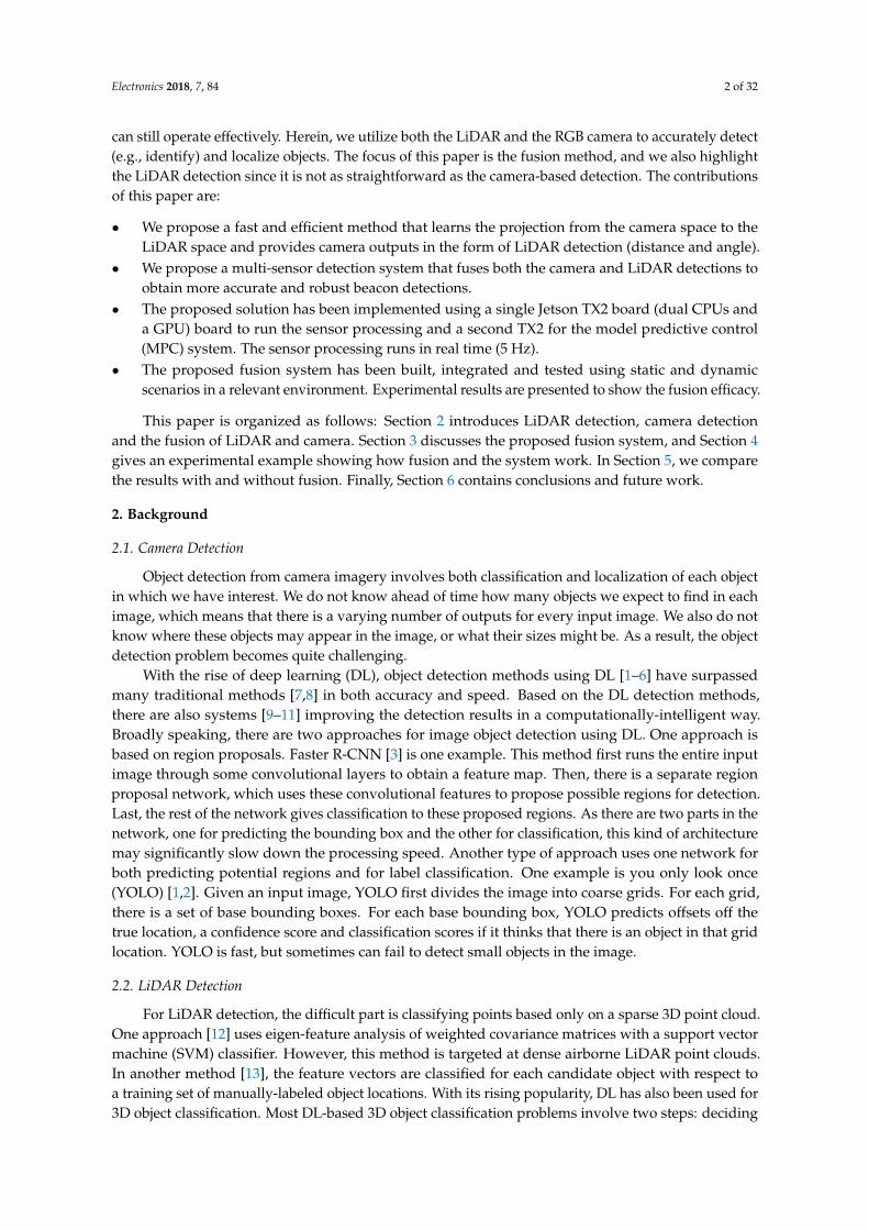
The proposed fusion system is shown in Figure 3. In this system, we first obtain images from thecamera, then through the camera object detection system, we estimate the bounding box coordinatesof beacons together with the confidence scores for each bounding box. Next, the detection boundingbox from the single camera is mapped through a neural network (NN) into a distance and angleestimate, in order to be able to fuse that information with the distance and angle estimates of theLiDAR processing.
On the other side, we have point cloud information from the LiDAR, then through LiDAR dataprocessing, we estimate the distance and angle information of the detected beacons by the LiDAR.Through the LiDAR processing, we also obtain a pseudo-confidence score. With the LiDAR detectionresults in the form of distance and angle from both the camera and LiDAR, we fuse them together to
Electronics 2018, 7, 84 6 of 32
obtain a final distance, angle and confidence score for each detection. We give more details about thisin Section 3.8.
In our application, the maximum speed of the vehicle is about 5 m per second. In order to haveenough reaction time for collision avoidance, the detection frequency needs to be 5 Hz or above.We accomplish this requirement for sensor processing on one NVIDIA Jetson TX2 and use another TX2for the MPC controller. More details are given in Section 3.2.
Figure 3. Proposed fusion system high-level block diagram.
3.2. Real-Time Implementation
To achieve the desired 5-Hz update rate for real-time performance, multiple compromises weremade to improve software speed enough to meet the requirements. Notably, a naive approachfor removal of ground points from the LiDAR point cloud was used instead of a more complex,and accurate, method. Furthermore, a linear SVM, with a limited feature set, was used as opposed toa kernel SVM or other non-linear methods. The specifics of these methods are covered in Section 3.6.
To manage intra-process communication between sensor drivers and signal processing functions,the Robot Operating System (ROS) was used [37]. ROS provides already-implemented sensor driversfor extracting point cloud and image data from the LiDAR and camera, respectively. Additionally,ROS abstracts and simplifies intra-process data transfer by using virtualized Transmission ControlProtocol (TCP) connections between the individual ROS processes, called nodes. As a consequenceof this method, multiple excess memory copies must be made, which begin to degrade performancewith large objects like LiDAR point clouds. To ameliorate this effect, ROS Nodelets [38] were usedfor appropriate LiDAR processes. Nodelets builds on ROS Nodes to provide a seamless interfacefor pooling multiple ROS processes into a single, multi-threaded process. This enables efficientzero-copy data transfers between signal processing steps for the high bandwidth LiDAR computations.This proved essential due to the limited resources of the TX2, with central processing unit (CPU)utilization averaging at over 95% even after Nodelets optimization.
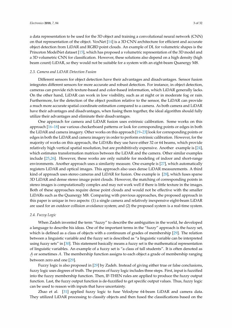
In Figure 4, the high-level flowchart of the relevant ROS nodes can be seen along with theirexecution location on the Jetson TX2’s hardware. The NVIDIA Jetson TX2 has a 256 CUDA (ComputeUnified Device Architecture) core GPU, a Dual CPU, 8 GB of memory and supports various interfacesincluding Ethernet [39]. As the most computationally-intensive operation, the camera CNN has theentire graphical processing unit (GPU) allocated to it. The sensor drivers, signal processing and fusionnodes are then relegated to the CPU. Due to the high core utilization from the LiDAR, care has to betaken that enough CPU resources are allocated to feed images to the GPU or significant throttling ofthe CNN can occur.
Electronics 2018, 7, 84 7 of 32
Figure 4. ROS dataflow on Jetson TX2.
3.3. Beacon
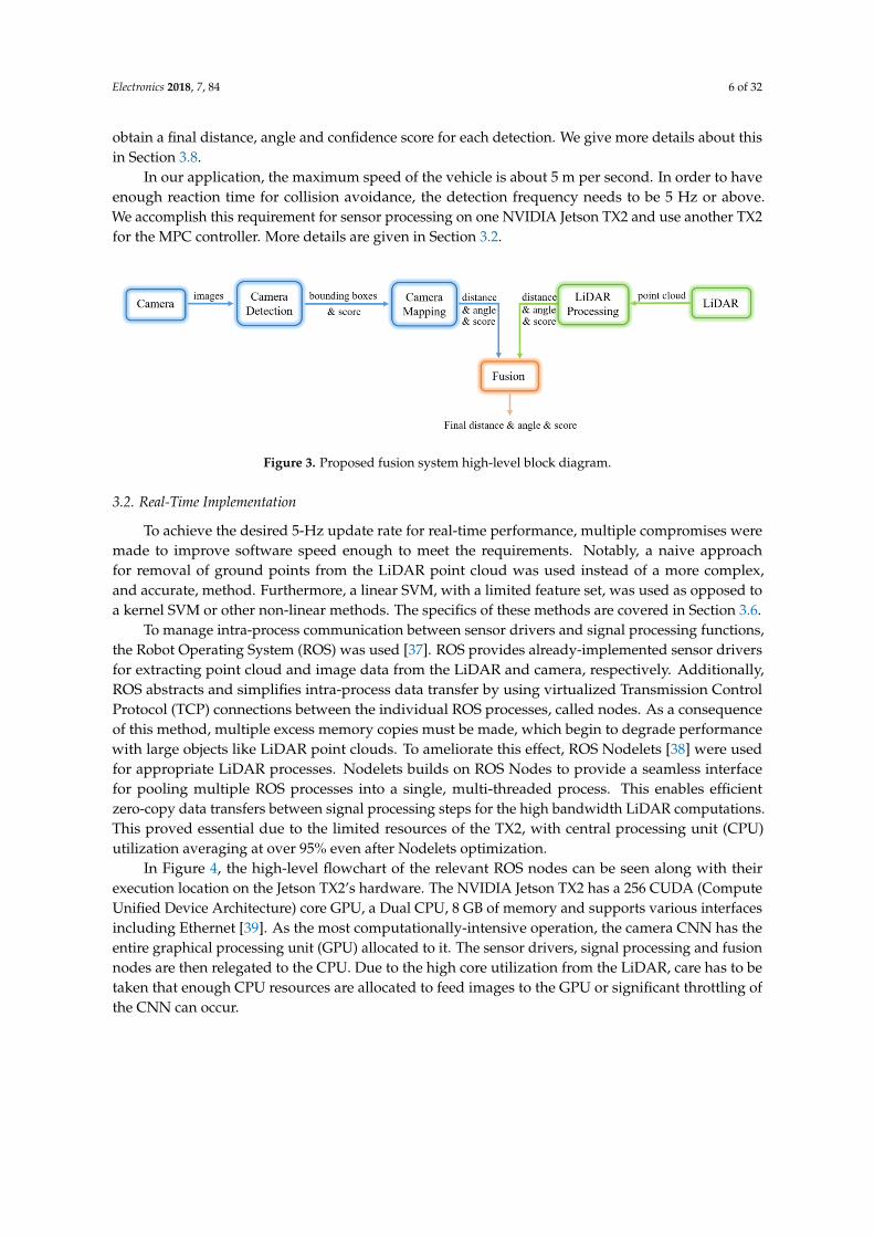
The beacon is constructed of a high-visibility 28” orange traffic cone with a 2” diameterhighly-reflective pole extending two meters vertically. A beacon is shown in Figure 5. The beaconpresents as a series of high intensity values in a LiDAR scan and thus provides a high signal levelcompared to most background objects. A beacon delineates an area in the industrial complex that isoff limits to the vehicle, usually to protect high-valued assets.
Figure 5. Beacon.
3.4. Camera Detection
Herein, we apply a deep-learning model called YOLO [1,2] to detect objects present in the singlecamera image. YOLO outperforms most other deep learning methods in speed, which is crucialfor our application. YOLO achieves such speed by combining both region and class predictioninto one network, unlike region-based methods [3,5,40], which have a separate network for regionproposals.
A large training dataset of beacon images presented in Section 4 was collected on different days,different times of day and weather conditions (e.g., full sun, overcast, etc.) and was hand-labeled by

Electronics 2018, 7, 84 8 of 32
our team members. Figure 6 shows how we draw bounding boxes and assign labels on an imagefrom the camera.
Figure 6. Labeling for camera detection.
The dataset we collected covers the camera’s full field of view (FOV) (−20◦ to 20◦ azimuth)and detection range (5 to 40 m) (FLIR Chameleon3 USB camera with Fujinon 6-mm lens). It reliablyrepresents the detection accuracy from different angles and distances. Figure 7 shows the markingson the ground that help us to locate the beacon at different angles and distances. These tests wereperformed early in the project to allow us to estimate the LiDAR detection accuracies.
(a) (b)
Figure 7. (a) Markings on the ground. (b) View from the camera. Markings on the ground covering thefull FOV and detection range of the camera.
All of the beacons have a highly consistent construction, with near-identical size,shape and coloring. These characteristics allow the detection algorithm to reliably recognize beaconsat a range of up to 40 m under a variety of lighting conditions. Figure 8 shows one example of thecamera detection of beacons.

Electronics 2018, 7, 84 9 of 32
Figure 8. Camera detection example. Best viewed in color.
3.5. LiDAR Front Guard
The LiDAR detection mode is designed to detect beacons. However, other objects can be in thedirect or near-direct path of the industrial vehicle. A front guard system is implemented with theLiDAR. Since many objects lack any bright points, thus being missed by the LiDAR beacon detection,we also employed a front-guard system, which clusters points in a rectangular area above the grounddirectly in front of the industrial vehicle. The front guard is then used to keep the vehicle from strikingobstacles or people. After ground point removal, any remaining points within a rectangular solidregion directly in front of the vehicle will be detected and reported to the control system.
3.6. LiDAR Beacon Detection
This section discusses the LiDAR’s beacon detection system.
3.6.1. Overview
The LiDAR data we collect are in the form of a three-dimensional (3D) and 360 degree field-of-view(FOV) point cloud, which consists of x, y, z coordinates, along with intensity and beam number(sometimes called ring number). The coordinates x, y and z represent the position of each point relativeto the origin centered within the LiDAR. Intensity represents the strength of returns and is an integerfor this model of LiDAR. Highly reflective objects such as metal or retro-reflective tape will have higherintensity values. The beam number represents in which beam the returned point is located. The LiDARwe use transmits eight beams. The beam numbers are shown in Figure 9. Assuming the LiDAR ismounted level to the ground, then Beam 7 is the top beam and is aimed upward approximately 3◦.Beam 6 points horizontally. The beams are spaced approximately 3◦ apart. Figure 10 shows one scanof the LiDAR point cloud. In this figure, the ground points are shown with black points. The beaconpresents as a series of closely-spaced points in the horizontal direction, as shown in the square.
General object detection in LiDAR is a difficult and unsolved problem in the computer visioncommunity. Objects appear at different scales based on their distance to the LiDAR, and they can beviewed from any angle. However, in our case, we are really only interested in detecting the beacons,which all have the same geometries. In our application, the industrial vehicle can only go so fast, so thatwe only need to detect beacons about 20 m away or closer. The beacons are designed to have verybright returns. However, other objects can also have bright returns in the scene, such as people wearingsafety vests with retro-reflective tape, or other industrial vehicles. Herein, we propose a system thatfirst identifies clusters of points in the scene that present with bright returns. Next, a linear SVMclassifier is used to differentiate the beacon clusters from non-beacon clusters.

Electronics 2018, 7, 84 10 of 32
Figure 9. LiDAR beam spacing visualization and beam numbering. The LiDAR is the small black boxon the left. Beam 6 is the horizontal beam (assuming the LiDAR is level).
Figure 10. Detection via LiDAR.
The LiDAR detection system works by utilizing intensity-based and density-based clustering(a modified DBSCAN algorithm) on the LiDAR point cloud. The system then examines all pointsnear the cluster centroid by extracting features and using a linear SVM to discriminate beacons fromnon-beacons. Details of these algorithm are discussed in the subsections below.
3.6.2. LiDAR Clustering
A modified DBSCAN clustering algorithm [41], which clusters based on point cloud density, aswell as intensity is used to cluster the bright points, as shown in Algorithm 1. The cluster parameter ε
was empirically determined to be 0.5 m based on the size of the beacon. Values much larger couldgroup two nearby beacons (or a beacon and another nearby object) together into one cluster, and wewanted to keep them as separate clusters.
In Equation (1), the distances are estimated using Euclidean distances with only the x(front-to-back) and y (left-to-right) coordinates. Effectively, this algorithm clusters bright LiDARpoints by projecting them down onto the x-y plane. Alternately, all three coordinates, x, y, zcould be used, but the features don not require this because they will be able to separate tall andshort objects. This approach is also more computationally efficient than using all three coordinates inthe clustering algorithm.

Electronics 2018, 7, 84 11 of 32
Algorithm 1: LiDAR bright pixel clustering.
Input: LiDAR point cloud P = {xj, yj, zj, ij, rj} with NP points.Input: High-intensity threshold: TH .Input: Cluster distance threshold: ε (meters).Input: Ground Z threshold: TG (meters).
Output: Cluster number for each bright point in the point cloud.
Remove non-return points:for each point in the point cloud do
Remove all non-return points (NaN’s) from the the point cloud.
Remove ground points:for each point in the modified point cloud do
Remove all points with Z-values below TG from the point cloud.
Remove non-bright points:for each point in the modified point cloud do
Remove all points with intensity values below TH from the point cloud.
Cluster bright points:Assign all points to Cluster 0.Set cl ← 0.for each point Pj in the modified point cloud do
if The point does not belong to a cluster thenAdd point to clusterIncrement the number of clusters: cl ← cl + 1.Assign Pj to cluster cl.Set the centroid of cluster cl to Pj.Scan through all remaining points and re-cluster if necessary.for each point Pm with j < m ≤ NP do
if Distance from point Pm to the centroid of cluster cl has distance < ε thenAdd Pm to cluster cl.Recalculate the centroid of cluster cl.
3.6.3. LiDAR Feature Extraction
To extract the features, the ground points must be removed before feature processing occurs,or else false alarms can occur. Since this industrial application has a smooth, flat area for the ground,we employ a simple vertical threshold to remove ground points. If this system were to be generalizedto areas with more varying ground conditions, ground estimation methods such as those in [42–47]could be utilized. However, for this particular application, this was not necessary.
Next, the point intensities are compared to an empirically-determined threshold. The beaconis designed so that it provides bright returns to the LiDAR via the retro-reflective vertical pole.This works well, but there are also other objects in the scene that can have high returns, such asother industrial vehicles with retro-reflective markings or workers wearing safety vests withretro-reflective stripes. In order to classify objects as beacons and non-beacons, hand-crafted featuresare utilized (these are discussed below). After ground-removal and thresholding the intensity points,we are left with a set of bright points. A second set of intensity points is also analyzed, which consistsof all of the non-ground points (e.g., the point cloud after ground removal). The points in the brightpoint cloud are clustered. Beacons appear as tall, thin objects, whereas all other objects are either not as

Electronics 2018, 7, 84 12 of 32
tall, or wider. We extract features around the cluster center in a small rectangular volume centered ateach object’s centroid. We also extract features using a larger rectangular volume also centered aroundthe objects centroid. Features include counting the number of bright points in each region, determiningthe x, y and z extents of the points in each region, etc. Beacons mainly have larger values in the smallerregion, while other objects have values in the larger regions.
The two regions are shown in Figure 11. The idea of using an inner and an outer analysis regionis that a beacon will mostly have bright points located in the inner analysis region, while other objects,such as humans, other industrial vehicles, etc., will extend into the outer regions. Equations (1) and (2)define whether a LiDAR point pj with coordinates
(xj, yj, zj
)is in the inner region or outer region,
respectively, where the object’s centroid has coordinates (xC, yC, zC). Reference Figure 11 fora top-down illustration of the inner and outer regions.
Figure 11 shows an example beacon return with the analysis windows superimposed. Both theinner and outer analysis regions have x and y coordinates centered at the centroid location. The inneranalysis region has a depth (x coordinate) of 0.5 m and a width (y coordinate) of 0.5 m, and the heightincludes all points with z coordinate values of −1.18 m and above. The outer region extends 2.0 min both x and y directions and has the same height restriction as the inner region. These values weredetermined based on the dimensions of the beacon and based on the LiDAR height. The parameters∆xI , ∆yI and zMIN define the inner region relative to the centroid coordinates. Similarly, the parameters∆xO, ∆yO and zMIN define the outer region relative to the centroid coordinates. A point is in the innerregion if: (
xC −∆xI
2
)≤ xj ≤
(xC +
∆xI2
)and(
yC −∆yI
2
)≤ yj ≤
(yC +
∆yI2
)and
zMIN ≥ zj,
(1)
and a point is in the outer region if:(xC −
∆xO2
)≤ xj ≤
(xC +
∆xO2
)and(
yC −∆yO
2
)≤ yj ≤
(yC +
∆yO2
)and
zMIN ≥ zj.
(2)
In order to be robust, we also extract features on the intensity returns. A linear SVM was trainedon a large number of beacon and non-beacon objects, and each feature was sorted based on its abilityto distinguish beacons from non-beacons. In general, there is a marked increase in performance, thenthe curve levels out. It was found that ten features were required to achieve very high detection ratesand low false alarms. These ten features were utilized in real time, and the system operates in real timeat the frame rate of the LiDAR, 5 Hz. The system was validated by first running on another large testset independent of the training set, with excellent performance as a result as presented in Section 3.6.4.Then, extensive field tests were used to further validate the results as presented in Section 4.
After detection, objects are then classified as beacons or non-beacons. These are appended totwo separate lists and reported by their distance in meters from the front of the industrial vehicle,their azimuth angle in degrees and their discriminate value. Through extensive experimentation,we can reliably see beacons in the LiDAR’s FOV from 3 to 20 m.
LiDAR feature extraction follows the overall algorithm shown in Algorithm 2. The input is theLiDAR point cloud P = {xj, yj, zj, ij, rj}, where j is the index variable for the j-th point, and x, y, z, iand r refer to the x point in meters, the y point in meters, the z point in meters, the intensity and thebeam number, respectively, for the j-th point. Note that all coordinates are relative to the center of the

Electronics 2018, 7, 84 13 of 32
LiDAR at point (0, 0, 0). The x coordinate is positive in front of the LiDAR, and negative behind. The ycoordinate is positive to the left of the LiDAR and negative to the right. The z coordinate is positiveabove the LiDAR and negative below.
Figure 11. LiDAR detection regions (inner and outer) visualized from a top-down view.
Algorithm 2: LiDAR high-level feature extraction preprocessing.
Input: LiDAR point cloud P = {xj, yj, zj, ij, rj}.Input: Low-intensity threshold: TL.Input: High-intensity threshold: TH .Input: Ground Z threshold: TG (meters).
Output: Feature vector f.
Remove non-return points:for each point in the point cloud do
Remove all non-return points (NaN’s) from the point cloud.
Remove ground points:for each point in the modified point cloud do
Remove all points with Z-values below TG from the point cloud.
Create threshold point clouds:Set PHT = ∅.Set PLT = ∅.for each point Pj in the modified point cloud do
if Point Pj has intensity ≥ TH thenAdd Pj to PHT .
if Point Pj has intensity ≥ TL thenAdd Pj to PLT .
Extract features:Extract features f using Algorithm 3.

Electronics 2018, 7, 84 14 of 32
In order to extract features for objects, any points that did not provide a return to the LiDARare removed. These points will present as NaN’s (not a number) in the LiDAR point cloud.Next, the estimated ground points are removed. The non-ground points are divided into twodata subsets: The high-threshold (HT) data and the low-threshold (LT) data. The HT data pointsonly contain high-intensity returns, while the LT data contain points greater than or equal to thelow-intensity threshold. Both data subsets do not contain any ground points. The high-intensitythreshold was set to 15 and the low-intensity threshold to zero. These threshold values weredetermined experimentally based on the examination of multiple beacon returns at various distances.
Algorithm 3: LiDAR feature extraction.
Input: LiDAR high-intensity point cloud PHT = {xj, yj, zj, ij, rj}.Input: LiDAR low-intensity point cloud PLT = {xj, yj, zj, ij, rj}.Input: Inner region x-extent: ∆xI (meters).Input: Inner region y-extent: ∆yI (meters).Input: Outer region x-extent: ∆xO (meters).Input: Outer region y-extent: ∆yO (meters).Input: LiDAR height above ground: ZL = 1.4 (meters).
Output: Feature vector f.
Cluster the high-intensity point cloud:for each point in p in the high-intensity point cloud do
Cluster points and determine cluster centers.
Calculate features:for each cluster center point c = (xC, yC, zC) in the point cloud do
Determine all points in PHT in the inner region using Equation (1), and calculate Features 1,13 and 17 from Table 1.
Determine all points in PHT in the outer region using Equation (2), and calculate Feature 4from Table 1.
Determine all points in PLT in the inner region using Equation (1), and calculate Features 6,7, 9 10, 11, 14, 16 and 18 from Table 1.
Determine all points in PLT in the outer region using Equation (2), and calculate Features 2,3, 5 8, 12, 15, 19 and 20 from Table 1.
Return f = [ f1, f2, f3, · · · , f20].
Table 1 describes the extracted features. For example, Feature 1 is generated from the highthreshold data, which consists solely of high-intensity points. The data is analyzed only forhigh-intensity points in the inner analysis region. This feature simply computes the Z (height) extent,that is, the maximum Z value minus the minimum Z value. Note that some of the features are onlyprocessed on certain beams, such as Feature 2. The features are listed in order of their discriminatepower in descending order, e.g., Feature 1 is the most discriminate, Feature 2 the next most discriminate,etc. Initially, it was unknown how effective the features would be. We started with 134 features,and these were ranked in order of their discriminating power using the score defined as:
SCORE = 500TP
TP + FN+ 500
TNTN + FP
(3)
where TP, TN, FP and FN are the number of true positives, true negatives, false positive and falsenegatives, respectively [48]. A higher score is better, and scores range from zero to 1000. This scorewas used since training with overall accuracy tended to highly favor one class and provided poor

Electronics 2018, 7, 84 15 of 32
generalizability, which may be a peculiarity of the chosen features and the training set. Figure 12 showsthe score values versus the number of features (where the features are sorted in descending score order.The operating point is shown for M = 20 features (circles in the plot). The features generalize fairlywell since the testing curve is similar to the training curve. In our system, using 20 features provideda good balance of performance versus computational complexity to compute the features. Each LiDARscan (5-Hz scan rate) requires calculating features for each cluster. Experimentation showed that atotal of 20 features was near the upper limit of what the processor could calculate and not degrade theLiDAR processing frame rate.
Table 1. Feature descriptions. Data subsets: HT = high threshold data. LT = low threshold data.The LiDAR rings are shown in Figure 9.
FeatureNumber
DataSubset
AnalysisRegion Description
1 HT Inner Extent of Z in cluster. Extent {Z} = max{Z} −min{Z}.
2 LT OuterMax of X and Y extents in cluster, Beam 7. This is max{extent{X}, extent{Y}}.Extent {X} = max{X} −min{X}. Extent {Y} = max{Y} −min{Y}.
3 LT OuterMax of X and Y extents in cluster, Beam 5. This is max{extent{X}, extent{Y}}.Extent {X} = max{X} −min{X}. Extent {Y} = max{Y} −min{Y}.
4 HT Outer Max{Z in cluster - LiDAR height}. Z is vertical (height) of LiDAR return.
5 LT Outer Extent of Z in cluster. Extent{Z}= max{Z} −min{Z}.
6 LT Inner Number of valid points in cluster, Beam 7.
7 LT InnerMax of X and Y extents in cluster, Beam 6. This is max{extent{X}, extent{Y}}.Extent {X} = max{X} −min{X}. Extent {Y} = max{Y} −min{Y}.
8 LT Outer Number of points in cluster, Beam 5.
9 LT Inner Extent of X in cluster. Extent{X} = max{X} −min{X}.
10 LT Inner Number of points in cluster, Beam 4.
11 LT Inner Number of points in cluster, Beam 5.
12 LT Outer Number of points in cluster, Beam 6.
13 HT Inner Number of points in cluster, Beam 6.
14 LT InnerMax of X and Y extents, Beam 5. This is max{extent{X}, extent{Y}}.Extent {X} = max{X} −min{X}. Extent {Y} = max{Y} −min{Y}.
15 LT Outer Number of points in cluster divided by the cluster radius in Beam 5.
16 LT Inner Extent of X in cluster. Extent {X} = max{X} −min{X}.
17 HT Inner Number of points in cluster, Beam 7.
18 LT Inner Number of points in cluster.
19 LT Outer Number of points in cluster.
20 LT Outer Extent of Z in cluster. Extent {Y} = max{Y} −min{Y}.

Electronics 2018, 7, 84 16 of 32
Figure 12. Score value versus number of concatenated features.
3.6.4. SVM LiDAR Beacon Detection
To detect the beacons in the 3D LiDAR point cloud, we use a linear SVM [49], which makesa decision based on a learned linear discriminant rule operating on the hand-crafted features we havedeveloped for differentiating beacons. Herein, liblinear was used to train the SVM [50]. A linear SVMoperates by finding the optimal linear combination of features that best separates the training data.If the M testing features for a testing instance are given by f = [ f1, f2, · · · , fM]T , where the superscriptT is a vector transpose operator, then the SVM evaluates the discriminant:
D = f ·w + b, (4)
where w is the SVM weight vector and b is the SVM bias term. Herein, M was chosen to be 20.Equation (4) applies a linear weight to each feature and adds a bias term. The discriminant isoptimized during SVM training. The SVM optimizes the individual weights in the weight vector tomaximize the margin and provide the best overall discriminant capability of the SVM. The bias termlets the optimal separating hyperplane drift from the origin. Figure 13 shows an example case withtwo features. In this case, the D = 0 hyperplane is the decision boundary. The D = +1 and D = −1hyperplanes are determined by the support vectors. The SVM only uses the support vectors to definethe optimal boundary.
The SVM was trained with beacon and non-beacon data extracted over multiple data collections.There were 13,190 beacon training instances and 15,209 non-beacon training instances. The test datahad 12,084 beacons and 5666 non-beacon instances.
In this work, M = 20 features were chosen. Each feature is first normalized by subtracting themean of the feature values from the training data and dividing each feature by four times the standarddeviation plus 10−5 (in order to prevent division by very small numbers). Subtracting the meanvalue centers the feature probability distribution function (PDF) around zero. Dividing by four times,the standard deviation maps almost all feature values into the range [−1, 1], because most of thevalues lie within ±4σk. The normalized features are calculated using:
f ′k =fk − µk
4σk + 10−5 (5)

Electronics 2018, 7, 84 17 of 32
where µk is the mean value of feature k and σk is the standard deviation of feature k for k = 1, 2, · · · , M.The mean and standard deviation are estimated from the training data and then applied to the test data.The final discriminant is computed using Equation (4) where the feature vector is the normalizedfeature vector.
Figure 13. SVM 2D example. The margin is the distance from the D = −1 to D = 1 hyperplanes.
The optimal feature weighs are shown in Figure 14. Since all the features are normalized, Features1, 3 and 8 have the most influence on the final discriminant function.
If the discriminant D ≤ 0, then the object is declared a beacon. Otherwise, it is declareda non-beacon (and ignored by the LiDAR beacon detection system). Once the SVM is trained,implementing the discriminant given in Equation (4) is trivial and uses minimal processing time.
Figure 15 shows the PDF of the LiDAR discriminant values for beacons and non-beacons,respectively. The PDFs are nearly linearly separable. The more negative the discriminant values,the more the object is beacon-like.

Electronics 2018, 7, 84 18 of 32
Figure 14. Optimal feature weights chosen by the SVM training optimizer.
Figure 15. LiDAR discriminant values.
3.7. Mapping
This section discusses the camera detection mapping from bounding box coordinates to distanceand angle. It also discusses the mapping of LiDAR discriminate value from the range [−∞, ∞] to [0, 1].
3.7.1. Camera Detection Mapping
The LiDAR and the camera both provide information on object detection, although in entirelydifferent coordinate spaces. The LiDAR provides accurate angle and range estimates with the
Electronics 2018, 7, 84 19 of 32
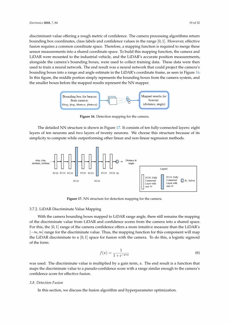
discriminant value offering a rough metric of confidence. The camera processing algorithms returnbounding box coordinates, class labels and confidence values in the range [0, 1]. However, effectivefusion requires a common coordinate space. Therefore, a mapping function is required to merge thesesensor measurements into a shared coordinate space. To build this mapping function, the camera andLiDAR were mounted to the industrial vehicle, and the LiDAR’s accurate position measurements,alongside the camera’s bounding boxes, were used to collect training data. These data were thenused to train a neural network. The end result was a neural network that could project the camera’sbounding boxes into a range and angle estimate in the LiDAR’s coordinate frame, as seen in Figure 16.In this figure, the middle portion simply represents the bounding boxes from the camera system, andthe smaller boxes before the mapped results represent the NN mapper.
Figure 16. Detection mapping for the camera.
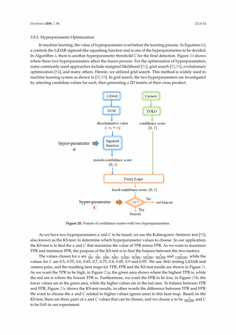
The detailed NN structure is shown in Figure 17. It consists of ten fully-connected layers: eightlayers of ten neurons and two layers of twenty neurons. We choose this structure because of itssimplicity to compute while outperforming other linear and non-linear regression methods.
Figure 17. NN structure for detection mapping for the camera.
3.7.2. LiDAR Discriminate Value Mapping
With the camera bounding boxes mapped to LiDAR range angle, there still remains the mappingof the discriminate value from LiDAR and confidence scores from the camera into a shared space.For this, the [0, 1] range of the camera confidence offers a more intuitive measure than the LiDAR’s[−∞, ∞] range for the discriminate value. Thus, the mapping function for this component will mapthe LiDAR discriminate to a [0, 1] space for fusion with the camera. To do this, a logistic sigmoidof the form:
f (x) =1
1 + e−α∗x (6)
was used. The discriminate value is multiplied by a gain term, α. The end result is a function thatmaps the discriminate value to a pseudo-confidence score with a range similar enough to the camera’sconfidence score for effective fusion.
3.8. Detection Fusion
In this section, we discuss the fusion algorithm and hyperparameter optimization.

Electronics 2018, 7, 84 20 of 32
3.8.1. Fusion Algorithm
With these two mapping components, a full pipeline can now be established to combine theLiDAR and camera data into forms similar enough for effective fusion. Using distance and angleinformation from both the camera and LiDAR, we can correlate LiDAR and camera detections together.Their confidence scores can then be fused as shown in Algorithm 4.
Algorithm 4: Fusion of LiDAR and Camera detection.
Input: Detection from LiDAR in the form of [distance, angle, pseudo-confidence score].Input: Detection from camera in the form of [distance, angle, confidence score].Input: Angular threshold: A for angle difference between fused camera and LiDAR detection.Input: Confidence threshold: C for final detection confidence score threshold.
Output: Fused detection in the form of [distance, angle, detection confidence].
for each detection from camera doif a corresponding LiDAR detection, with angle difference less than A, exists then
Fuse by using the distance and angle from LiDAR, and combine confidence scoresusing fuzzy logic to determine the fused detection confidence.
elseCreate a new detection from camera, using the distance, angle and confidence scorefrom camera as the final detection result.
for each LiDAR detection that does not have a corresponding camera detection doCreate a new detection from LiDAR, using the distance, angle and confidence score fromLiDAR as the final detection result.
for each fused detection doRemove detections with final confidences below the C confidence threshold.
Return fused detection results.
In this algorithm, the strategy for fusion of the distance and angle estimates is different fromthe fusion of confidence scores, which is shown in Figure 18. In the process of distance and anglefusion, for each camera detection, when there is a corresponding detection from LiDAR, we will usethe distance and angle information from LiDAR, as LiDAR can provide much more accurate positionestimation. When there is no corresponding LiDAR detection, we will use the distance, angle andconfidence score from the camera to create a new detection. For each detection from LiDAR that doesnot have corresponding camera detection, we will use the distance, angle and confidence score fromLiDAR as the final result. For confidence score fusion, we use fuzzy logic to produce a final confidencescore when there is corresponding camera and LiDAR detection. The fuzzy rules used in the fuzzylogic system are as follows:
1. If the LiDAR confidence score is high, then the probability for detection is high.2. If the camera confidence score is high, then the probability for detection is high.3. If the LiDAR confidence score is medium, then the probability for detection is medium.4. If the LiDAR confidence score is low and the camera confidence score is medium, then the
probability for detection is medium.5. If the LiDAR confidence score is low and the camera confidence score is low, then the probability
for detection is low.
The fuzzy rules are chosen in this way because of the following reasons: First, if either the LiDARor the camera shows a high confidence in their detection, then the detections are very likely to be true.This is the reason for Rules 1 and 2: the LiDAR is robust at detection up to about 20 m. Within that

Electronics 2018, 7, 84 21 of 32
range, the confidence score from the LiDAR is usually high or medium. Beyond that range, the valuewill drop to low. This is the reason for Rule 3. Third, beyond the 20-m detection range, the system willsolely rely on the camera for detection. This is the reason for Rules 4 and 5.
Figure 19 shows the process of using fuzzy logic to combine the confidence scores from the cameraand LiDAR. The camera input, LiDAR input and detection output are fuzzified into fuzzy membershipfunctions as shown in Figure 19a–c. The output is shown in Figure 19d. In this example, when theconfidence score from the LiDAR is 80 and the score from the camera is 20, by applying the fivepre-defined fuzzy rules, the output detection score is around 56.
(a) (b)
Figure 18. (a) Fusion of distances and angles. (b) Fusion of confidence scores. Fusion of distances,angles and confidence scores from the camera and LiDAR.
(a) (b)
(c) (d)
Figure 19. (a) Fuzzy membership function for camera. (b) Fuzzy membership function for LiDAR.(c) Fuzzy membership function for detection. (d) Fuzzy logic output. Combination of confidence scoresfrom the camera and LiDAR using fuzzy logic. Figure best viewed in color.
Electronics 2018, 7, 84 22 of 32
3.8.2. Hyperparameter Optimization
In machine learning, the value of hyperparameter is set before the learning process. In Equation (6),α controls the LiDAR sigmoid-like squashing function and is one of the hyperparameters to be decided.In Algorithm 4, there is another hyperparameter threshold C for the final detection. Figure 20 showswhere these two hyperparameters affect the fusion process. For the optimization of hyperparameters,some commonly-used approaches include marginal likelihood [51], grid search [52,53], evolutionaryoptimization [54], and many others. Herein, we utilized grid search. This method is widely used inmachine learning system as shown in [52,53]. In grid search, the two hyperparameters are investigatedby selecting candidate values for each, then generating a 2D matrix of their cross product.
Figure 20. Fusion of confidence scores with two hyperparameters.
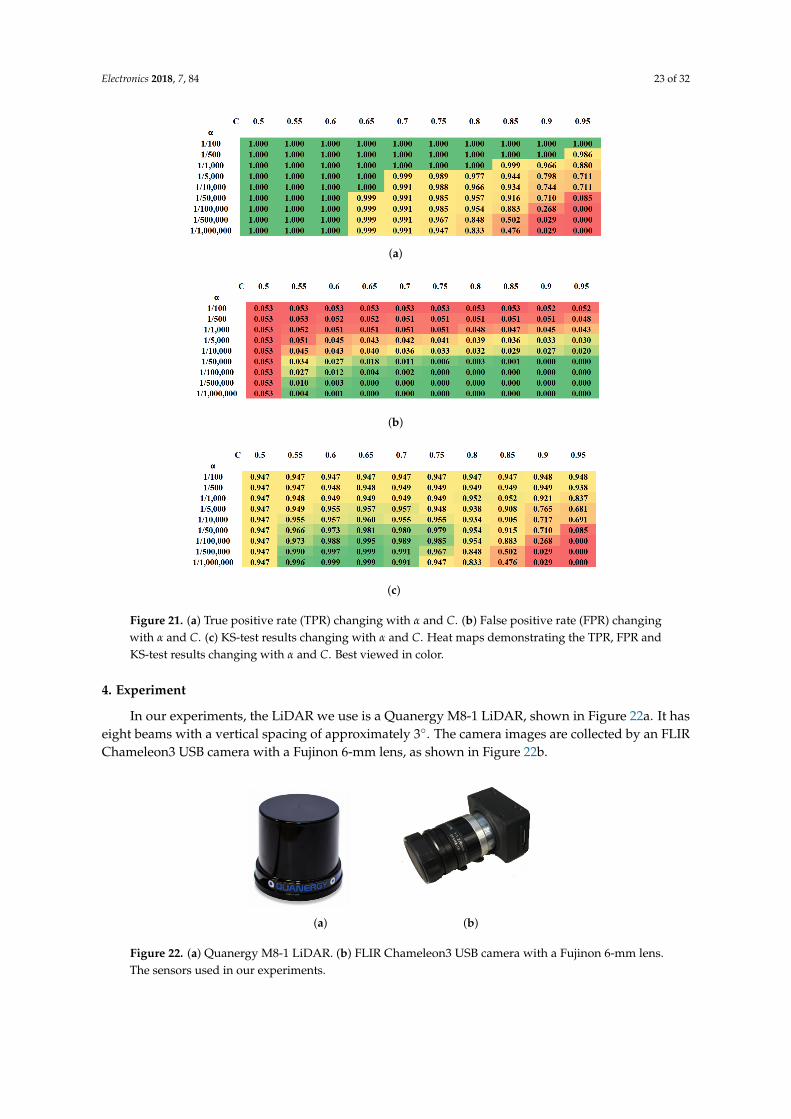
As we have two hyperparameters α and C to be tuned, we use the Kolmogorov–Smirnov test [55],also known as the KS-test, to determine which hyperparameter values to choose. In our application,the KS-test is to find the α and C that maximize the value of TPR minus FPR. As we want to maximizeTPR and minimize FPR, the purpose of the KS-test is to find the balance between the two metrics.
The values chosen for α are 1100 , 1
500 , 11000 , 1
5000 , 110,000 , 1
50,000 , 1100,000 , 1
500,000 and 11,000,000 , while the
values for C are 0.5, 0.55, 0.6, 0.65, 0.7, 0.75, 0.8, 0.85, 0.9 and 0.95. We use 3641 testing LiDAR andcamera pairs, and the resulting heat maps for TPR, FPR and the KS-test results are shown in Figure 21.As we want the TPR to be high, in Figure 21a, the green area shows where the highest TPR is, whilethe red are is where the lowest TPR is. Furthermore, we want the FPR to be low, in Figure 21b; thelower values are in the green area, while the higher values are in the red area. To balance between TPRand FPR, Figure 21c shows the KS-test results, in other words the difference between TPR and FPR.We want to choose the α and C related to higher values (green area) in this heat map. Based on theKS-test, there are three pairs of α and C values that can be chosen, and we choose α to be 1
500,000 and Cto be 0.65 in our experiment.
Electronics 2018, 7, 84 23 of 32
(a)
(b)
(c)
Figure 21. (a) True positive rate (TPR) changing with α and C. (b) False positive rate (FPR) changingwith α and C. (c) KS-test results changing with α and C. Heat maps demonstrating the TPR, FPR andKS-test results changing with α and C. Best viewed in color.
4. Experiment
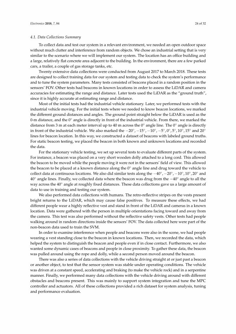
In our experiments, the LiDAR we use is a Quanergy M8-1 LiDAR, shown in Figure 22a. It haseight beams with a vertical spacing of approximately 3◦. The camera images are collected by an FLIRChameleon3 USB camera with a Fujinon 6-mm lens, as shown in Figure 22b.
(a) (b)
Figure 22. (a) Quanergy M8-1 LiDAR. (b) FLIR Chameleon3 USB camera with a Fujinon 6-mm lens.The sensors used in our experiments.
Electronics 2018, 7, 84 24 of 32
4.1. Data Collections Summary
To collect data and test our system in a relevant environment, we needed an open outdoor spacewithout much clutter and interference from random objects. We chose an industrial setting that is verysimilar to the scenario where we will implement our system. The location has an office building anda large, relatively flat concrete area adjacent to the building. In the environment, there are a few parkedcars, a trailer, a couple of gas storage tanks, etc.
Twenty extensive data collections were conducted from August 2017 to March 2018. These testsare designed to collect training data for our system and testing data to check the system’s performanceand to tune the system parameters. Many tests consisted of beacons placed in a random position in thesensors’ FOV. Other tests had beacons in known locations in order to assess the LiDAR and cameraaccuracies for estimating the range and distance. Later tests used the LiDAR as the “ground truth”,since it is highly accurate at estimating range and distance.
Most of the initial tests had the industrial vehicle stationary. Later, we performed tests with theindustrial vehicle moving. For the initial tests where we needed to know beacon locations, we markedthe different ground distances and angles. The ground point straight below the LiDAR is used as the0-m distance, and the 0◦ angle is directly in front of the industrial vehicle. From there, we marked thedistance from 3 m at each meter interval up to 40 m across the 0◦ angle line. The 0◦ angle is directlyin front of the industrial vehicle. We also marked the −20◦,−15◦,−10◦,−5◦, 0◦, 5◦, 10◦, 15◦ and 20◦
lines for beacon location. In this way, we constructed a dataset of beacons with labeled ground truths.For static beacon testing, we placed the beacon in both known and unknown locations and recordedthe data.
For the stationary vehicle testing, we set up several tests to evaluate different parts of the system.For instance, a beacon was placed on a very short wooden dolly attached to a long cord. This allowedthe beacon to be moved while the people moving it were not in the sensors’ field of view. This allowedthe beacon to be placed at a known distance along the 0◦ angle line and drug toward the vehicle tocollect data at continuous locations. We also did similar tests along the −40◦,−20◦,−10◦, 10◦, 20◦ and40◦ angle lines. Finally, we collected data where the beacon was drug from the −40◦ angle to all theway across the 40◦ angle at roughly fixed distances. These data collections gave us a large amount ofdata to use in training and testing our system.
We also performed data collections with humans. The retro-reflective stripes on the vests presentbright returns to the LiDAR, which may cause false positives. To measure these effects, we haddifferent people wear a highly reflective vest and stand in front of the LiDAR and cameras in a knownlocation. Data were gathered with the person in multiple orientations facing toward and away fromthe camera. This test was also performed without the reflective safety vests. Other tests had peoplewalking around in random directions inside the sensors’ FOV. The data collected here were part of thenon-beacon data used to train the SVM.
In order to examine interference when people and beacons were also in the scene, we had peoplewearing a vest standing close to the beacon in known locations. Then, we recorded the data, whichhelped the system to distinguish the beacon and people even if in close contact. Furthermore, we alsowanted some dynamic cases of beacons and people in close proximity. To gather these data, the beaconwas pulled around using the rope and dolly, while a second person moved around the beacon.
There was also a series of data collections with the vehicle driving straight at or just past a beaconor another object, to test that the sensor system was stable under operating conditions. The vehiclewas driven at a constant speed, accelerating and braking (to make the vehicle rock) and in a serpentinemanner. Finally, we performed many data collections with the vehicle driving around with differentobstacles and beacons present. This was mainly to support system integration and tune the MPCcontroller and actuators. All of these collections provided a rich dataset for system analysis, tuningand performance evaluation.

Electronics 2018, 7, 84 25 of 32
4.2. Camera Detection Training
Training images for YOLO also include images taken by a Nikon D7000 camera and images fromPASCAL VOC dataset [56]. The total number of training images is around 25,000.
The network structure of YOLO is basically the same as the default setting. One difference is thenumber of filters in the last layer. This number is related to the number of object categories we aretrying to detect and the number of base bounding boxes for each of the grid sections into which YOLOdivides the image. For example, we can divide each image into 13 by 13 grids. For each grid, YOLOpredicts five bounding boxes, and for each bounding box, there are 5 + N parameters (N representsthe number of categories to be predicted). As a result, the last layer filter size is 13× 13× 5× (5 + N).Another difference is that we change the learning rate to 10−5 to avoid divergence.
4.3. LiDAR Detection Training
The LiDAR data were processed through a series of steps. We implemented a ground clutterremoval algorithm to keep ground points from giving us false alarms, to avoid high reflections fromreflective paints on the ground and to reduce the size of our point cloud. Clusters of points are groupedinto distinct objects and are classified using an SVM. The SVM is trained using a large set of data thathave beacons and non-beacon objects. The LiDAR data were divided into two disjoint sets: trainingand testing. In the training dataset, there were 13,190 beacons and 15,209 non-beacons. The testingdataset contained 5666 beacons and 12,084 non-beacons. The confusion matrices for training andtesting are shown in Tables 2 and 3. The results show good performance for the training and testingdatasets. Both datasets show over 99.7% true positives (beacons) and around 93% true negatives(non-beacons).
Table 2. LiDAR training confusion matrix.
Beacon Non-Beacon
Beacon 13,158 32
Non-Beacon 610 14,599
Table 3. LiDAR testing confusion matrix.
Beacon Non-Beacon
Beacon 5653 13
Non-Beacon 302 11,782
5. Results and Discussion
5.1. Camera Detection Mapping Results
Camera and LiDAR detections generate both different types of data and data on different scales.The LiDAR generates range and angle estimates, while the camera generates bounding boxes.The LiDAR discriminant score can be any real number, while the camera confidence score is a realnumber in the range [0, 1]. The data from camera detection are first mapped into the form of distanceand range, the same form as the data reported from LiDAR. We can accomplish this conversion fairlyaccurately because we know the true size of the beacon. The data collected for mapping cover theentire horizontal FOV of the camera, which is −20◦ to 20◦ relative to the front of the industrial vehicle.The distance covered is from 3 to 40 m, which is beyond the maximum detection range of our LiDARdetection algorithm. We collected around 3000 pairs of camera and LiDAR detection for training of themapping NN and 400 pairs for testing.

Electronics 2018, 7, 84 26 of 32
From Figure 23, we observe that the larger the x-coordinate, the larger the angle from the camera,and the larger the size of the bounding box, the nearer the object to the camera. From our training data,we see that the bounding box’s x-coordinate has an approximately linear relationship with the LiDARdetection angle, as shown in Figure 24a. We also observe that the size of the bounding box fromthe camera detection has a nearly negative exponential relationship with the distance from LiDARdetection as shown in Figure 24b. To test these relationships, we ran least squares fitting algorithms toestimate coefficients for a linear fit between the [Xmin, Xmax] of the camera bounding box and theLiDAR angle and for an exponential fit between the [Width, Height] and the LiDAR estimated distance.
Figure 23. One sample frame with three different bounding boxes.
Herein, we compare the NN and linear regression result methods for angle estimation, and wealso compare the results using NN and exponential curve fitting method for distance. The results areshown in Table 4. The table shows the mean squared error (MSE) using both the NN and the linearregression for the angle estimation, as well as the MSE for distance estimation. The table also reportsthe coefficient of determination, or r2 scores [57]. The r2 scores show a high measure of goodness of fitfor the NN approximations. We find that the NN provides more accurate predictions on both distanceand angle.
Table 4. Mapping analysis. The best results are shown in bold.
Angle (Degrees) Distance (Meters)
NN Linear Regression NN Exponential Curve Fitting
Mean Squared Error (MSE) 0.0467 0.0468 0.0251 0.6278
r2 score 0.9989 0.9989 0.9875 0.9687
5.2. Camera Detection Results
In order to see how well the camera works on its own for reporting distance and angle forits detections, 400 testing images are processed. We compare the mapping results with the LiDARdetection, which is treated as the ground-truth. The results are shown in Figure 25. From Figure 25a,we can see that the camera can fairly accurately predict the angle with a maximum error around 3◦,and this only happens near the image edges. On the other hand, the camera’s distance prediction hasrelatively large errors, as shown in Figure 25b. Its maximum error is around 1 m, which happens whenthe distance is around 6 m, 9 m, 15 m and 18 m.

Electronics 2018, 7, 84 27 of 32
(a) Bounding box Xmin from the camera vs. the anglefrom LiDAR. Xmin units are pixels, and angle unitsare degrees.
(b) Bounding box Xmin from the camera vs. the anglefrom LiDAR. The bounding box width is pixels, and thedistance is meters.
Figure 24. Scatter plots of camera/LiDAR training data for fusion. (a) Camera bounding box Xmin vs.LiDAR estimated angle. (b) Camera bounding box width vs. LiDAR estimated distance.
5.3. Fusion Results
We also compare the true positive detections, false positive detections and false negative detectionsusing only LiDAR data with linear SVM method, only camera image results with YOLO and theproposed fusion method. The results are shown in Tables 5 and 6.
In Tables 5 and 6, TPR, FPR and FNR are calculated by Equations (7a) to (7c), respectively, in whichTP is the number of true positives (the number of true beacons detected), TN is the number of truenegatives (the number of non-beacons detected correctly), FP is the number of false positive (there isan object detected as a beacon that is not a beacon) and FNis the number of false negatives (there isa beacon, but we have no detection).
True Positive Rate (TPR) =TP
TP + FN(7a)
False Positive Rate (FPR) =FP
FP + TN(7b)
False Negative Rate (FNR) =FN
TP + FN(7c)

Electronics 2018, 7, 84 28 of 32
Table 5. Fusion performance: 3 to 20-m range. The best results in bold.
LiDAR Only Camera Only Fusion
True Positive Rate (TPR) 93.90% 97.60% 97.60%
False Positive Rate (FPR) 27.00% 0.00% 6.69%
False Negative Rate (FNR) 6.10% 2.40% 2.40%
Table 6. Fusion performance: 20 to 40-m range. The best results in bold.
Camera Only Fusion
True Positive Rate (TPR) 94.80% 94.80%
False Positive Rate (FPR) 0.00% 0.00%
False Negative Rate (FNR) 5.20% 5.20%
(a)
(b)
Figure 25. (a) Angle error of the camera. (b) Distance error of the camera. Camera errors.
From these results, one can see that from the camera, there are more detections within its FOVup to 40 m, while its estimation of position, especially for distance, is not accurate. The camera,however, can fail more quickly in rain or bad weather, so we cannot always rely on the camera in badweather [58,59]. On the other hand, the LiDAR has accurate position estimation for each point, butthe current LiDAR processing cannot reliably detect beyond about 20 m; and its false detection rate
Electronics 2018, 7, 84 29 of 32
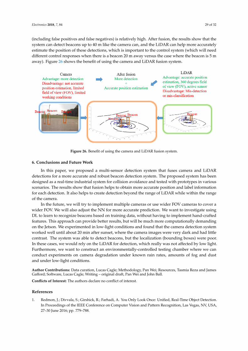
(including false positives and false negatives) is relatively high. After fusion, the results show that thesystem can detect beacons up to 40 m like the camera can, and the LiDAR can help more accuratelyestimate the position of these detections, which is important to the control system (which will needdifferent control responses when there is a beacon 20 m away versus the case where the beacon is 5 maway). Figure 26 shows the benefit of using the camera and LiDAR fusion system.
Figure 26. Benefit of using the camera and LiDAR fusion system.
6. Conclusions and Future Work
In this paper, we proposed a multi-sensor detection system that fuses camera and LiDARdetections for a more accurate and robust beacon detection system. The proposed system has beendesigned as a real-time industrial system for collision avoidance and tested with prototypes in variousscenarios. The results show that fusion helps to obtain more accurate position and label informationfor each detection. It also helps to create detection beyond the range of LiDAR while within the rangeof the camera.
In the future, we will try to implement multiple cameras or use wider FOV cameras to cover awider FOV. We will also adjust the NN for more accurate prediction. We want to investigate usingDL to learn to recognize beacons based on training data, without having to implement hand-craftedfeatures. This approach can provide better results, but will be much more computationally demandingon the Jetson. We experimented in low-light conditions and found that the camera detection systemworked well until about 20 min after sunset, where the camera images were very dark and had littlecontrast. The system was able to detect beacons, but the localization (bounding boxes) were poor.In these cases, we would rely on the LiDAR for detection, which really was not affected by low light.Furthermore, we want to construct an environmentally-controlled testing chamber where we canconduct experiments on camera degradation under known rain rates, amounts of fog and dustand under low-light conditions.
Author Contributions: Data curation, Lucas Cagle; Methodology, Pan Wei; Resources, Tasmia Reza and JamesGafford; Software, Lucas Cagle; Writing – original draft, Pan Wei and John Ball.
Conflicts of Interest: The authors declare no conflict of interest.
References
1. Redmon, J.; Divvala, S.; Girshick, R.; Farhadi, A. You Only Look Once: Unified, Real-Time Object Detection.In Proceedings of the IEEE Conference on Computer Vision and Pattern Recognition, Las Vegas, NV, USA,27–30 June 2016; pp. 779–788.
Electronics 2018, 7, 84 30 of 32
2. Redmon, J.; Farhadi, A. YOLO9000: Better, Faster, Stronger. In Proceedings of the IEEE Conference onComputer Vision and Pattern Recognition, Honolulu, HI, USA, 21–26 July 2017; pp. 6517–6525.
3. Ren, S.; He, K.; Girshick, R.; Sun, J. Faster R-CNN: Towards real-time object detection with region proposalnetworks. IEEE Trans. Pattern Anal. Mach. Intell. 2017, 39, 1137–1149. [CrossRef] [PubMed]
4. Szegedy, C.; Reed, S.; Erhan, D.; Anguelov, D.; Ioffe, S. Scalable, high-quality object detection. arXiv 2014,arXiv:1412.1441.
5. Dai, J.; Li, Y.; He, K.; Sun, J. R-FCN: Object detection via region-based fully convolutional networks. InProceedings of the Neural Information Processing Systems 2016, Barcelona, Spain, 5–10 December 2016;pp. 379–387.
6. Liu, W.; Anguelov, D.; Erhan, D.; Szegedy, C.; Reed, S.; Fu, C.Y.; Berg, A.C. SSD: Single shot multiboxdetector. In Proceedings of the European Conference on Computer Vision, Amsterdam, The Netherlands,8–16 October 2016; pp. 21–37.
7. Dalal, N.; Triggs, B. Histograms of Oriented Gradients for Human Detection. In Proceedings of the IEEEComputer Society Conference on Computer Vision and Pattern Recognition, San Diego, CA, USA, 20–25June 2005; pp. 886–893.
8. Felzenszwalb, P.F.; Girshick, R.B.; McAllester, D.; Ramanan, D. Object detection with discriminatively trainedpart-based models. IEEE Trans. Pattern Anal. Mach. Intell. 2010, 32, 1627–1645. [CrossRef] [PubMed]
9. Wei, P.; Ball, J.E.; Anderson, D.T.; Harsh, A.; Archibald, C. Measuring Conflict in a Multi-Source Environmentas a Normal Measure. In Proceedings of the IEEE 6th International Workshop on Computational Advancesin Multi-Sensor Adaptive Processing (CAMSAP), Cancun, Mexico, 13–16 December 2015; pp. 225–228.
10. Wei, P.; Ball, J.E.; Anderson, D.T. Multi-sensor conflict measurement and information fusion. In SignalProcessing, Sensor/Information Fusion, and Target Recognition XXV; International Society for Optics andPhotonics: Bellingham, WA, USA, 2016; Volume 9842, p. 98420F.
11. Wei, P.; Ball, J.E.; Anderson, D.T. Fusion of an Ensemble of Augmented Image Detectors for Robust ObjectDetection. Sensors 2018, 18, 894. [CrossRef] [PubMed]
12. Lin, C.H.; Chen, J.Y.; Su, P.L.; Chen, C.H. Eigen-feature analysis of weighted covariance matrices for LiDARpoint cloud classification. ISPRS J. Photogr. Remote Sens. 2014, 94, 70–79. [CrossRef]
13. Golovinskiy, A.; Kim, V.G.; Funkhouser, T. Shape-Based Recognition of 3D Point Clouds in UrbanEnvironments. In Proceedings of the IEEE 12th International Conference on Computer Vision, Kyoto, Japan,29 September–2 October 2009; pp. 2154–2161.
14. Maturana, D.; Scherer, S. Voxnet: A 3d Convolutional Neural Network for Real-Time Object Recognition.In Proceedings of the IEEE/RSJ International Conference on Intelligent Robots and Systems (IROS), Hamburg,Germany, 28 September–2 October 2015; pp. 922–928.
15. Wu, Z.; Song, S.; Khosla, A.; Yu, F.; Zhang, L.; Tang, X.; Xiao, J. 3d Shapenets: A Deep Representation forVolumetric Shapes. In Proceedings of the IEEE Conference on Computer Vision and Pattern Recognition,Boston, MA, USA, 7–12 June 2015; pp. 1912–1920.
16. Gong, X.; Lin, Y.; Liu, J. Extrinsic calibration of a 3D LIDAR and a camera using a trihedron. Opt. Laser Eng.2013, 51, 394–401. [CrossRef]
17. Park, Y.; Yun, S.; Won, C.S.; Cho, K.; Um, K.; Sim, S. Calibration between color camera and 3D LIDARinstruments with a polygonal planar board. Sensors 2014, 14, 5333–5353. [CrossRef] [PubMed]
18. García-Moreno, A.I.; Gonzalez-Barbosa, J.J.; Ornelas-Rodriguez, F.J.; Hurtado-Ramos, J.B.; Primo-Fuentes,M.N. LIDAR and panoramic camera extrinsic calibration approach using a pattern plane. In MexicanConference on Pattern Recognition; Springer: Berlin, Germany, 2013; pp. 104–113.
19. Levinson, J.; Thrun, S. Automatic Online Calibration of Cameras and Lasers. In Proceedings of the Robotics:Science and Systems, Berlin, Germany, 24–28 June 2013.
20. Gong, X.; Lin, Y.; Liu, J. 3D LIDAR-camera extrinsic calibration using an arbitrary trihedron. Sensors 2013,13, 1902–1918. [CrossRef] [PubMed]
21. Napier, A.; Corke, P.; Newman, P. Cross-Calibration of Push-Broom 2d Lidars and Cameras in Natural Scenes.In Proceedings of the IEEE International Conference on Robotics and Automation (ICRA), Karlsruhe,Germany, 6–10 May 2013; pp. 3679–3684.
22. Pandey, G.; McBride, J.R.; Savarese, S.; Eustice, R.M. Automatic extrinsic calibration of vision and lidar bymaximizing mutual information. J. Field Robot. 2015, 32, 696–722. [CrossRef]

Electronics 2018, 7, 84 31 of 32
23. Castorena, J.; Kamilov, U.S.; Boufounos, P.T. Autocalibration of LIDAR and Optical Cameras via EdgeAlignment. In Proceedings of the IEEE International Conference on Acoustics, Speech and Signal Processing(ICASSP), Shanghai, China, 20–25 March 2016; pp. 2862–2866.
24. Li, J.; He, X.; Li, J. 2D LiDAR and Camera Fusion in 3D Modeling of Indoor Environment. In Proceedings ofthe IEEE National Aerospace and Electronics Conference (NAECON), Dayton, OH, USA, 15–19 June 2015;pp. 379–383.
25. Zhang, Q.; Pless, R. Extrinsic Calibration of a Camera and Laser Range Finder (Improves Camera Calibration).In Proceedings of the IEEE/RSJ International Conference on Intelligent Robots and Systems, Sendai, Japan,28 September–2 October 2004; pp. 2301–2306.
26. Vasconcelos, F.; Barreto, J.P.; Nunes, U. A minimal solution for the extrinsic calibration of a camera anda laser-rangefinder. IEEE Trans. Pattern Anal. Mach. Intell. 2012, 34, 2097–2107. [CrossRef] [PubMed]
27. Mastin, A.; Kepner, J.; Fisher, J. Automatic Registration of LIDAR and Optical Images of Urban Scenes.In Proceedings of the IEEE Conference on Computer Vision and Pattern Recognition, Miami, FL, USA,20–25 June 2009; pp. 2639–2646.
28. Maddern, W.; Newman, P. Real-Time Probabilistic Fusion of Sparse 3D LIDAR and Dense Stereo.In Proceedings of the IEEE/RSJ International Conference on Intelligent Robots and Systems (IROS),Daejeon, Korea, 9–14 October 2016; pp. 2181–2188.
29. Zadeh, L.A. Fuzzy sets. Inf. Control 1965, 8, 338–353. [CrossRef]30. Ross, T.J. Fuzzy Logic with Engineering Applications; John Wiley & Sons: Hoboken, NJ, USA, 2010.31. Zhao, G.; Xiao, X.; Yuan, J. Fusion of Velodyne and Camera Data for Scene Parsing. In Proceedings of the
15th International Conference on Information Fusion (FUSION), Singapore, 9–12 July 2012; pp. 1172–1179.32. Liu, J.; Jayakumar, P.; Stein, J.; Ersal, T. A Multi-Stage Optimization Formulation for MPC-based Obstacle
Avoidance in Autonomous Vehicles Using a LiDAR Sensor. In Proceedings of the ASME Dynamic Systemsand Control Conference, Columbus, OH, USA, 28–30 October 2015.
33. Alrifaee, B.; Maczijewski, J.; Abel, D. Sequential Convex Programming MPC for Dynamic VehicleCollision Avoidance. In Proceedings of the IEEE Conference on Control TEchnology and Applications,Mauna Lani, HI, USA, 27–30 August 2017.
34. Anderson, S.J.; Peters, S.C.; Pilutti, T.E.; Iagnemma, K. An Optimal-control-based Framework for TrajectoryPlanning, Thread Assessment, and Semi-Autonomous Control of Passenger Vehicles in Hazard AvoidanceScenarios. Int. J. Veh. Auton. Syst. 2010, 8, 190–216.
35. Liu, Y.; Davenport, C.; Gafford, J.; Mazzola, M.; Ball, J.; Abdelwahed, S.; Doude, M.; Burch, R. Development ofA Dynamic Modeling Framework to Predict Instantaneous Status of Towing Vehicle Systems; SAE Technical Paper;SAE International: Warrendale, PA, USA; Troy, MI, USA, 2017.
36. Davenport, C.; Liu, Y.; Pan, H.; Gafford, J.; Abdelwahed, S.; Mazzola, M.; Ball, J.E.; Burch, R.F. A kinematicmodeling framework for prediction of instantaneous status of towing vehicle systems. SAE Int. J. Passeng.Cars Mech. Syst. 2018. [CrossRef]
37. Quigley, M.; Gerkey, B.; Conley, K.; Faust, J.; Foote, T.; Leibs, J.; Berger, E.; Wheeler, R.; Ng, A. ROS: Anopen-source Robot Operating System. In Proceedings of the IEEE Conference on Robotics and Automation(ICRA) Workshop on Open Source Robotics, Kobe, Japan, 12–17 May 2009.
38. ROS Nodelet. Available online: http://wiki.ros.org/nodelet (accessed on 22 April 2018).39. JETSON TX2 Technical Specifications. Available online: https://www.nvidia.com/en-us/autonomous-
machines/embedded-systems-dev-kits-modules/ (accessed on 5 March 2018).40. Girshick, R. Fast R-CNN. arXiv 2015, arXiv:1504.08083.41. Ester, M.; Kriegel, H.P.; Sander, J.; Xu, X. A density-based algorithm for discovering clusters in large spatial
databases with noise. In Proceedings of the Second International Conference on Knowledge Discovery andData Mining, Portland, OR, USA, 2–4 August 1996; pp. 226–231.
42. Wang, L.; Zhang, Y. LiDAR Ground Filtering Algorithm for Urban Areas Using Scan Line BasedSegmentation. arXiv 2016, arXiv:1603.00912. [CrossRef]
43. Meng, X.; Currit, N.; Zhao, K. Ground filtering algorithms for airborne LiDAR data: A review of criticalissues. Remote Sens. 2010, 2, 833–860. [CrossRef]
44. Rummelhard, L.; Paigwar, A.; Nègre, A.; Laugier, C. Ground estimation and point cloud segmentation usingSpatioTemporal Conditional Random Field. In Proceedings of the Intelligent Vehicles Symposium (IV), LosAngeles, CA, USA, 11–14 June 2017; pp. 1105–1110.

Electronics 2018, 7, 84 32 of 32
45. Rashidi, P.; Rastiveis, H. Ground Filtering LiDAR Data Based on Multi-Scale Analysis of Height DifferenceThreshold. Int. Arch. Photogramm. Remote Sens. Spat. Inf. Sci. 2017, XLII-4/W4, 225–229. [CrossRef]
46. Chang, Y.; Habib, A.; Lee, D.; Yom, J. Automatic classification of lidar data into ground and non-groundpoints. Int. Arch. Photogr. Remote Sens. 2008, 37, 463–468.
47. Miadlicki, K.; Pajor, M.; Saków, M. Ground plane estimation from sparse LIDAR data for loader cranesensor fusion system. In Proceedings of the 2017 22nd International Conference on Methods and Models inAutomation and Robotics (MMAR), Miedzyzdroje, Poland, 28–31 August 2017; pp. 717–722.
48. Lillywhite, K.; Lee, D.J.; Tippetts, B.; Archibald, J. A feature construction method for general objectrecognition. Pattern Recognit. 2013, 46, 3300–3314. [CrossRef]
49. Vapnik, V. Statistical Learning Theory; Wiley: New York, NY, USA, 1998.50. Fan, R.; Chang, K.; Hsieh, C. LIBLINEAR: A library for large linear classification. J. Mach. Learn. Res. 2008,
9, 1871–1874.51. Zorzi, M.; Chiuso, A. Sparse plus low rank network identification: A nonparametric approach. Automatica
2017, 76, 355–366. [CrossRef]52. Chicco, D. Ten quick tips for machine learning in computational biology. BioData Min. 2017, 10, 35.
[CrossRef] [PubMed]53. Hsu, C.W.; Chang, C.C.; Lin, C.J. A Practical Guide to Support Vector Classification; Technical Report; National
Taiwan University: Taiwan, China, 2010.54. Olson, R.S.; Urbanowicz, R.J.; Andrews, P.C.; Lavender, N.A.; Moore, J.H. Automating biomedical data
science through tree-based pipeline optimization. In Proceedings of the European Conference on theApplications of Evolutionary Computation, Porto, Portugal, 30 March–1 April 2016; pp. 123–137.
55. Chakravarty, I.M.; Roy, J.; Laha, R.G. Handbook of Methods of Applied Statistics; McGraw-Hill: New York, NY,USA, 1967.
56. Everingham, M.; Van Gool, L.; Williams, C.K.; Winn, J.; Zisserman, A. The pascal visual object classes (voc)challenge. Int. J. Comput. Vis. 2010, 88, 303–338. [CrossRef]
57. Draper, N.R.; Smith, H. Applied Regression Analysis; John Wiley & Sons: Hoboken, NJ, USA, 2014; Volume 326.58. Larochelle, V.; Bonnier, D.; Roy, G.; Simard, J.R.; Mathieu, P. Performance assessment of various imaging
sensors in fog. In Proceedings of the International Society for Optical Engineering, Aspen, CO, USA, 10–13May 1998; pp. 66–81.
59. Park, D.; Ko, H. Fog-degraded image restoration using characteristics of RGB channel in single monocularimage. In Proceedings of the IEEE International Conference on Consumer Electronics, Las Vegas, NV, USA,13–16 January 2012; pp. 139–140.
c© 2018 by the authors. Licensee MDPI, Basel, Switzerland. This article is an open accessarticle distributed under the terms and conditions of the Creative Commons Attribution(CC BY) license (http://creativecommons.org/licenses/by/4.0/).