lics 2012 short papers - tau
TRANSCRIPT
LICS 2012 Short Papers

2
Table of Contents
Short Papers Selected from Regular Submissions
A New Order-theoretic Characterisation of the Polytime Computable Functions . . . . . . . . . . . . . . . . . . . . . . . . . . . . . . . . . . . . 7Martin Avanzini, Naohi Eguchi and Georg Moser
Views: Compositional Reasoning for Concurrent Programs . . . . . . . . . . . . . . . . . . . . . . . . . . . . . . . . . . . . . . . . . . . . . . . . . . . . . . . . . 9Thomas Dinsdale-Young, Lars Birkedal, Philippa Gardner, Matthew Parkinson and Hongseok Yang
Herbrand-Confluence for Cut Elimination in Classical First Order Logic . . . . . . . . . . . . . . . . . . . . . . . . . . . . . . . . . . . . . . . . . . . . 11Stefan Hetzl and Lutz Straßburger
The Refined Calculus of Inductive Construction: Parametricity and Abstraction . . . . . . . . . . . . . . . . . . . . . . . . . . . . . . . . . . . . 13Chantal Keller and Marc Lasson
Undecidable First-Order Theories of A�ne Geometries . . . . . . . . . . . . . . . . . . . . . . . . . . . . . . . . . . . . . . . . . . . . . . . . . . . . . . . . . . . . . 15Antti Kuusisto, Jeremy Meyers and Jonni Virtema
Canonical Progress Measures for Parity Games . . . . . . . . . . . . . . . . . . . . . . . . . . . . . . . . . . . . . . . . . . . . . . . . . . . . . . . . . . . . . . . . . . . . . 17Konstantinos Mamouras
Down the Borel Hierarchy: Solving Muller Games via Safety Games . . . . . . . . . . . . . . . . . . . . . . . . . . . . . . . . . . . . . . . . . . . . . . . . 19Daniel Neider, Roman Rabinovich and Martin Zimmermann
Interaction Graphs: Additives . . . . . . . . . . . . . . . . . . . . . . . . . . . . . . . . . . . . . . . . . . . . . . . . . . . . . . . . . . . . . . . . . . . . . . . . . . . . . . . . . . . . . . 21Thomas Seiller
Ribbon Proofs for Separation Logic . . . . . . . . . . . . . . . . . . . . . . . . . . . . . . . . . . . . . . . . . . . . . . . . . . . . . . . . . . . . . . . . . . . . . . . . . . . . . . . . 23John Wickerson, Mike Dodds and Matthew Parkinson
Short Papers from the Specific Short Papers Call
Logical Bell Inequalities . . . . . . . . . . . . . . . . . . . . . . . . . . . . . . . . . . . . . . . . . . . . . . . . . . . . . . . . . . . . . . . . . . . . . . . . . . . . . . . . . . . . . . . . . . . . 27Samson Abramsky and Lucien Hardy
Approximations of Conjunctive Queries . . . . . . . . . . . . . . . . . . . . . . . . . . . . . . . . . . . . . . . . . . . . . . . . . . . . . . . . . . . . . . . . . . . . . . . . . . . . 29Pablo Barcelo, Leonid Libkin and Miguel Angel Romero Orth
Complete Axiomatizations of Fragments of Monadic Second-Order Logic on Finite Trees . . . . . . . . . . . . . . . . . . . . . . . . . . . 31Amelie Gheerbrant and Balder ten Cate
Uniform Polytime Computable Operators on Univariate Real Analytic Functions . . . . . . . . . . . . . . . . . . . . . . . . . . . . . . . . . . . 33Akitoshi Kawamura, Norbert Muller, Martin Ziegler and Carsten Rosnick
A metric analogue of Stone duality for Markov processes . . . . . . . . . . . . . . . . . . . . . . . . . . . . . . . . . . . . . . . . . . . . . . . . . . . . . . . . . . . 35Kim Larsen, Radu Mardare and Prakash Panangaden
The Comprehension Cube. . . . . . . . . . . . . . . . . . . . . . . . . . . . . . . . . . . . . . . . . . . . . . . . . . . . . . . . . . . . . . . . . . . . . . . . . . . . . . . . . . . . . . . . . . 37Daniel Leivant
On the expressivity of linear logic subsystems characterizing polynomial time . . . . . . . . . . . . . . . . . . . . . . . . . . . . . . . . . . . . . . . 39Matthieu Perrinel
3

4

Short Papers Selected from Regular Submissions
5

6
7
A New Order-theoretic Characterisation of thePolytime Computable Functions
Martin Avanzini∗, Naohi Eguchi† and Georg Moser∗∗Institute of Computer ScienceUniversity of Innsbruck, Austria
Email: {martin.avanzini,georg.moser}@uibk.ac.at†Mathematical Institute
Tohoku University, JapanEmail: [email protected]
I. INTRODUCTION
In this work we are concerned with the complexity analysisof term rewrite systems (TRSs for short) and the ramificationsof such an analysis in implicit computational complexity.Details and full proofs can be found in our technical report [1].The foundation of rewriting is equational logic and termrewrite systems are conceivable as sets of directed equations.A natural way to measure the complexity of a TRS R is tomeasure the length of computations in R. More precisely theruntime complexity of a TRS relates the maximal lengths ofderivations to the size of the initial term, whose arguments aresupposed to be values, i.e., irreducible. Indeed, runtime com-plexity is an invariant cost model [2]: all functions computedby a TRS allow realisations within polynomial overhead on astandard models of computation, like Turing machines.
We propose a new order, the small polynomial path order(sPOP∗ for short) that induces polynomial (innermost) runtimecomplexities. The proposed order embodies the principle ofpredicative recursion set forth by Bellantoni and Cook [3]in their alternative characterisation B of the polynomial timecomputable functions (FP for short). Let us make this ideaprecise. We are assuming that the arguments of every functionare partitioned in to normal and safe ones. Notationally wewrite f(t1, . . . , tk ; tk+1, . . . , tk+l) where normal arguments areto the left, and safe arguments to the right of the semicolon. Wedefine a restriction B
wsc
of B, where crucially the underlyingcomposition scheme is replaced by a weaker form, disallowingcomposition under normal arguments. Defining rules of B
wsc
are given in Fig. 1. The distinctive feature that permits only theformulation of feasible functions is of course the separationof normal (the recursion parameters) from safe arguments (theplaces for substituting recursive results). Due to a variation ofa result by Handley and Wainer, we have that B
wsc
capturesall the polytime functions [4].
Theorem 1. Every function from Bwsc
is polytime computable.Vice versa, B
wsc
contains every polytime computable function.
Suppose the definition of a TRS R is based on the equations
This work is partially supported by FWF (Austrian Science Fund) projectI-608-N18 and a grant of the University of Innsbruck.
in Bwsc
. By its precise definition we can measure the runtimecomplexity based on the number d of nested applications ofsafe recursion (SRN), that is, for such predicative recursiveTRSs R of degree d, the runtime complexity is bounded bya polynomial of degree d. To decide whether a TRS R ispredicative recursive of degree d, we have devised the ordersPOP∗. In fact this order theoretic characterisation is moreliberal than B
wsc
, but main principles that allow a preciseestimation of runtime complexities remain reflected.
II. MOTIVATION AND RELATED WORK
It is clear that an order-theoretic characterisation of pred-icative recursion is obtained as a restriction of the recur-sive path order. Predicative recursion stems from a carefulanalysis of primitive recursion and the recursive path order(with multiset status) characterises the class of primitiverecursive functions [5]. The light multiset path order (LMPOfor short) proposed by Marion [6] tames this recursive pathorder by embodying the principle of predicative recursion.LMPO captures FP, but captured rewrite systems do not admitpolynomially runtime complexities in general. Polynomialruntime complexity analysis is an active research area inrewriting, see [7] for an overview. In particular, variations ofdependency pairs for complexity analysis [8], [9], [10], alsoin combination with modularity results [11], established majorbreakthroughs. Since LMPO is inapplicable in this setting, theauthors were motivated to present a restriction of LMPO, thepolynomial path order (POP∗ for short) [12]. This order is stillcomplete for FP, but also induces feasible bounds on runtimecomplexities of rewrite systems. Still, POP∗ suffers from thefact that the precise degree of the polynomial certificate cannotbe estimated. The order sPOP∗ eliminates this final weakness.
We also want to mention Bonfante et. al. [13] whererestricted classes of polynomial interpretations are studiedthat can also precisely bind the runtime complexity of TRSs.Although incomparable to our technique, unarguably suchsemantic techniques admit a better intentionality, but aredifficult to implement efficiently in an automated setting. Inour complexity tool TCT1 we see sPOP∗ as a fruitful and fast
1TCT is open source. The interested reader might play with the web interfaceavailable at http://cl-informatik.uibk.ac.at/software/tct.
8
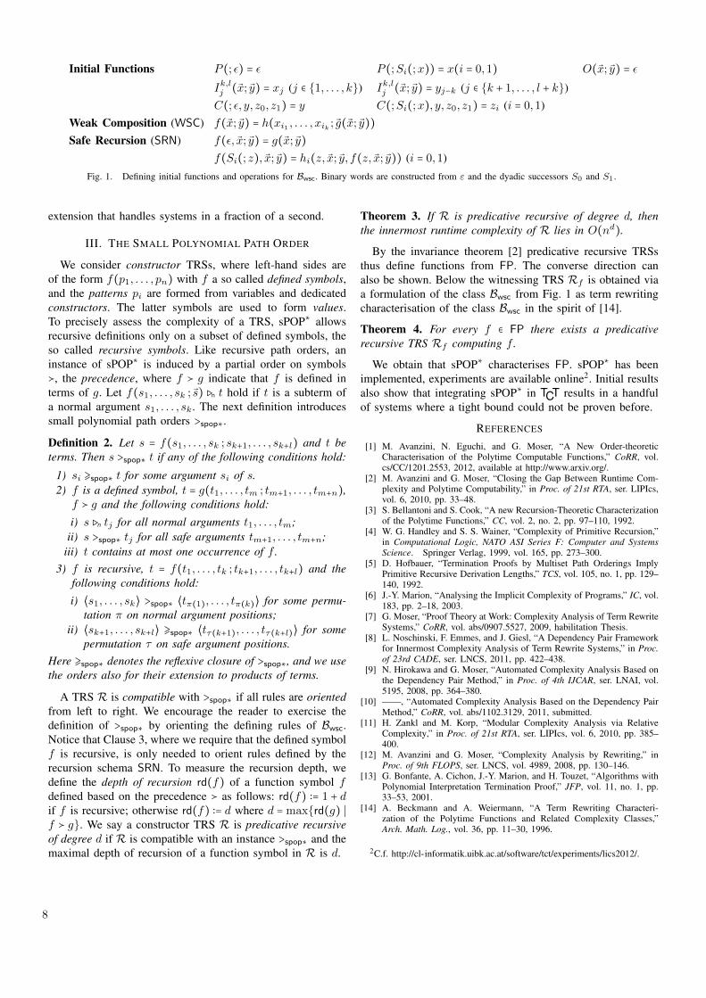
Initial Functions P (; ✏) = ✏ P (;Si(;x)) = x(i = 0,1) O(�x; �y) = ✏Ik,lj (�x; �y) = xj (j ∈ {1, . . . , k}) Ik,lj (�x; �y) = yj−k (j ∈ {k + 1, . . . , l + k})C(; ✏, y, z0, z1) = y C(;Si(;x), y, z0, z1) = zi (i = 0,1)
Weak Composition (WSC) f(�x; �y) = h(xi1 , . . . , xik ; �g(�x; �y))Safe Recursion (SRN) f(✏, �x; �y) = g(�x; �y)
f(Si(; z), �x; �y) = hi(z, �x; �y, f(z, �x; �y)) (i = 0,1)Fig. 1. Defining initial functions and operations for B
wsc
. Binary words are constructed from " and the dyadic successors S0 and S1.
extension that handles systems in a fraction of a second.
III. THE SMALL POLYNOMIAL PATH ORDER
We consider constructor TRSs, where left-hand sides areof the form f(p1, . . . , pn) with f a so called defined symbols,and the patterns pi are formed from variables and dedicatedconstructors. The latter symbols are used to form values.To precisely assess the complexity of a TRS, sPOP∗ allowsrecursive definitions only on a subset of defined symbols, theso called recursive symbols. Like recursive path orders, aninstance of sPOP∗ is induced by a partial order on symbols�, the precedence, where f � g indicate that f is defined interms of g. Let f(s1, . . . , sk ; �s) �n t hold if t is a subterm ofa normal argument s1, . . . , sk. The next definition introducessmall polynomial path orders >
spop∗.Definition 2. Let s = f(s1, . . . , sk ; sk+1, . . . , sk+l) and t beterms. Then s >
spop∗ t if any of the following conditions hold:1) si �spop∗ t for some argument si of s.2) f is a defined symbol, t = g(t1, . . . , tm ; tm+1, . . . , tm+n),
f � g and the following conditions hold:i) s �n tj for all normal arguments t1, . . . , tm;
ii) s >spop∗ tj for all safe arguments tm+1, . . . , tm+n;
iii) t contains at most one occurrence of f .3) f is recursive, t = f(t1, . . . , tk ; tk+1, . . . , tk+l) and the
following conditions hold:i) �s1, . . . , sk� >spop∗ �t⇡(1), . . . , t⇡(k)� for some permu-
tation ⇡ on normal argument positions;ii) �sk+1, . . . , sk+l� �spop∗ �t⌧(k+1), . . . , t⌧(k+l)� for some
permutation ⌧ on safe argument positions.Here �
spop∗ denotes the reflexive closure of >spop∗, and we use
the orders also for their extension to products of terms.
A TRS R is compatible with >spop∗ if all rules are oriented
from left to right. We encourage the reader to exercise thedefinition of >
spop∗ by orienting the defining rules of Bwsc
.Notice that Clause 3, where we require that the defined symbolf is recursive, is only needed to orient rules defined by therecursion schema SRN. To measure the recursion depth, wedefine the depth of recursion rd(f) of a function symbol fdefined based on the precedence � as follows: rd(f) ∶= 1 + dif f is recursive; otherwise rd(f) ∶= d where d =max{rd(g) �f � g}. We say a constructor TRS R is predicative recursiveof degree d if R is compatible with an instance >
spop∗ and themaximal depth of recursion of a function symbol in R is d.
Theorem 3. If R is predicative recursive of degree d, thenthe innermost runtime complexity of R lies in O(nd).
By the invariance theorem [2] predicative recursive TRSsthus define functions from FP. The converse direction canalso be shown. Below the witnessing TRS Rf is obtained viaa formulation of the class B
wsc
from Fig. 1 as term rewritingcharacterisation of the class B
wsc
in the spirit of [14].
Theorem 4. For every f ∈ FP there exists a predicativerecursive TRS Rf computing f .
We obtain that sPOP∗ characterises FP. sPOP∗ has beenimplemented, experiments are available online2. Initial resultsalso show that integrating sPOP∗ in TCT results in a handfulof systems where a tight bound could not be proven before.
REFERENCES
[1] M. Avanzini, N. Eguchi, and G. Moser, “A New Order-theoreticCharacterisation of the Polytime Computable Functions,” CoRR, vol.cs/CC/1201.2553, 2012, available at http://www.arxiv.org/.
[2] M. Avanzini and G. Moser, “Closing the Gap Between Runtime Com-plexity and Polytime Computability,” in Proc. of 21st RTA, ser. LIPIcs,vol. 6, 2010, pp. 33–48.
[3] S. Bellantoni and S. Cook, “A new Recursion-Theoretic Characterizationof the Polytime Functions,” CC, vol. 2, no. 2, pp. 97–110, 1992.
[4] W. G. Handley and S. S. Wainer, “Complexity of Primitive Recursion,”in Computational Logic, NATO ASI Series F: Computer and SystemsScience. Springer Verlag, 1999, vol. 165, pp. 273–300.
[5] D. Hofbauer, “Termination Proofs by Multiset Path Orderings ImplyPrimitive Recursive Derivation Lengths,” TCS, vol. 105, no. 1, pp. 129–140, 1992.
[6] J.-Y. Marion, “Analysing the Implicit Complexity of Programs,” IC, vol.183, pp. 2–18, 2003.
[7] G. Moser, “Proof Theory at Work: Complexity Analysis of Term RewriteSystems,” CoRR, vol. abs/0907.5527, 2009, habilitation Thesis.
[8] L. Noschinski, F. Emmes, and J. Giesl, “A Dependency Pair Frameworkfor Innermost Complexity Analysis of Term Rewrite Systems,” in Proc.of 23rd CADE, ser. LNCS, 2011, pp. 422–438.
[9] N. Hirokawa and G. Moser, “Automated Complexity Analysis Based onthe Dependency Pair Method,” in Proc. of 4th IJCAR, ser. LNAI, vol.5195, 2008, pp. 364–380.
[10] ——, “Automated Complexity Analysis Based on the Dependency PairMethod,” CoRR, vol. abs/1102.3129, 2011, submitted.
[11] H. Zankl and M. Korp, “Modular Complexity Analysis via RelativeComplexity,” in Proc. of 21st RTA, ser. LIPIcs, vol. 6, 2010, pp. 385–400.
[12] M. Avanzini and G. Moser, “Complexity Analysis by Rewriting,” inProc. of 9th FLOPS, ser. LNCS, vol. 4989, 2008, pp. 130–146.
[13] G. Bonfante, A. Cichon, J.-Y. Marion, and H. Touzet, “Algorithms withPolynomial Interpretation Termination Proof,” JFP, vol. 11, no. 1, pp.33–53, 2001.
[14] A. Beckmann and A. Weiermann, “A Term Rewriting Characteri-zation of the Polytime Functions and Related Complexity Classes,”Arch. Math. Log., vol. 36, pp. 11–30, 1996.
2C.f. http://cl-informatik.uibk.ac.at/software/tct/experiments/lics2012/.

9
Views: Compositional Reasoning for ConcurrencyThomas Dinsdale-Young†, Lars Birkedal⇤, Philippa Gardner†, Matthew Parkinson‡, Hongseok Yang§
†Imperial College London, ⇤IT University of Copenhagen, ‡Microsoft Research Cambridge, §University of Oxford
Abstract—We present a framework for reasoning composition-
ally about concurrent programs. At its core is the notion of a
view: an abstraction of the state that takes account of the possible
interference due to other threads. Threads’ views are composable,
and an update to the state by one thread must preserve the
views of other threads. Existing and novel concurrency reasoning
systems can be expressed as instances of our framework, and can
be proved sound by appeal to a general soundness result.
I. INTRODUCTION
There has been a recent flurry of research activity on typesystems and program logics for reasoning modularly aboutprograms with dynamically allocated, shared mutable state.Type systems have been extended with linear types and relatedcapability system that enforce a mixture of local and globalproperties. Program logics, extending separation logic, havebeen developed to reason about various notions of sharing:for sequential languages, by combining with types and variousframe rules; for concurrent languages by adding invariant orrelational reasoning.
These developments have led to increasingly elaboratereasoning systems, each introducing new features to tacklespecific applications of modular reasoning and new metatheoryto justify these features. Despite their ad hoc nature, thesesystems employ a common approach to compositionality. Theyprovide thread-specific abstractions of the state, which embodyenough information to prove the behaviour of a thread whilstallowing for the possible behaviours of other threads. We in-troduce a general framework for these abstractions, identifyingthe properties necessary for sound, compositional reasoning.
Our fundamental idea is that threads have different viewsof the machine. Intuitively, a thread’s view consists of infor-mation about the current state of the machine, the right ofthe thread to modify the state as long as the environment’sview is stable (invariant) with respect to such changes, and thethread’s right to the stability of its own view with respect tochanges being made by the environment. Threads’ views canbe composed, which ensures that the rights and informationheld by different threads are compatible with each other.
A thread’s view provides a partial, abstract description ofthe state of the machine. It is partial in that it only describesthe state relevant to the thread. It is abstract in that the verifiercan use additional information to help with the reasoning, suchas types, ghost state or permissions. Such instrumentation hasno representation in the concrete state but is a useful fiction forthe verifier. To relate the program logic with the operationalsemantics, we require that a view can be reified to a set ofconcrete machine states. Using reification, we prove a generalsoundness result, which we have formally verified in Coq.
To illustrate the essential compositionality of views, con-sider a command C that updates the view p to the view q. Forcompositional reasoning, we would require that C updates p⇤rto q ⇤ r, where r represents any view held by the environmentand ⇤ is the composition operation on views. Traditionalapproaches in separation logic have achieved this by enforcingthat commands satisfy so-called locality conditions [1]. Wetake the alternative approach of embedding compositionalityinto the meaning of “C updates p to q”: for all r, it must updatep⇤ r to q ⇤ r. We show that this interpretation, which has beenused for formulating separation logics for concurrency andfor higher-order languages, gives a simpler and more generalmetatheory for logics for concurrent programs.
A crucial implication of this interpretation is that viewsshould be stable with respect to any operation that a threadwith a consistent view could perform. At one extreme, stabilitycan be enforced by disjointness between views: one thread canaccess variable x, say, while the other cannot have anything todo with x. At the other, stability can be enforced by invariantproperties: both threads may agree that x always has type bool,for instance. In the middle ground lie many logics that allowcontrolled sharing. Views capture this whole spectrum.
In this middle ground, the logic of concurrent abstract pred-icates [2] (CAP) models interference with rely and guaranteerelations, which pervade the soundness proof. The rely relationis used to describe the interference that a thread must expectfrom the environment, and assertions are required to be stable(invariant) under the rely. The guarantee relation constrains(somewhat conservatively) the possible updates that a threadmay make, to ensure that it cannot do anything the environ-ment does not expect. In the views framework, we simply takeviews to be the stable assertions. The guarantee constraintis enforced by the embedding of compositionality in thesemantics, which permits any operation that the environmentexpects. In Kripke models of type theories, the future worldrelation plays a similar role to the rely in describing possibleupdates, and is treated similarly in the views framework.
The views framework distils the essence of compositionalreasoning. In [3], we consider a range of examples as in-stantiations of our framework, including simple type systemsand separation logics, type systems with recursive types andunique references, a combination of separation logic and atype system in the spirit of [4], and CAP [2].
The framework is already being used to develop logicsfor advanced language features. CAP has been extended withhigher-order features and the soundness of this uses theviews framework extended with step-indexing [5]. Views havebeen extended to reason about C] with interesting permission
10
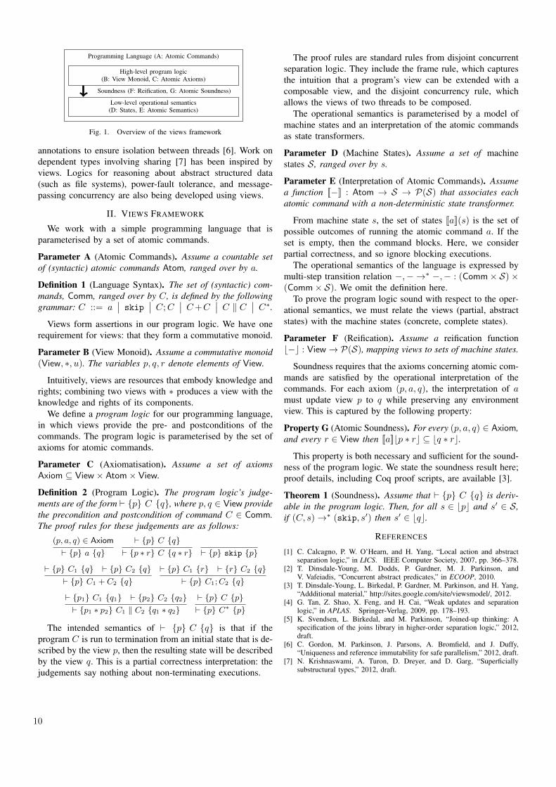
Programming Language (A: Atomic Commands)
High-level program logic(B: View Monoid, C: Atomic Axioms)
Soundness (F: Reification, G: Atomic Soundness)
Low-level operational semantics(D: States, E: Atomic Semantics)
Fig. 1. Overview of the views framework
annotations to ensure isolation between threads [6]. Work ondependent types involving sharing [7] has been inspired byviews. Logics for reasoning about abstract structured data(such as file systems), power-fault tolerance, and message-passing concurrency are also being developed using views.
II. VIEWS FRAMEWORK
We work with a simple programming language that isparameterised by a set of atomic commands.
Parameter A (Atomic Commands). Assume a countable setof (syntactic) atomic commands Atom, ranged over by a.
Definition 1 (Language Syntax). The set of (syntactic) com-mands, Comm, ranged over by C, is defined by the followinggrammar: C ::= a
�� skip�� C;C
�� C+C�� C k C
�� C⇤.
Views form assertions in our program logic. We have onerequirement for views: that they form a commutative monoid.
Parameter B (View Monoid). Assume a commutative monoid(View, ⇤, u). The variables p, q, r denote elements of View.
Intuitively, views are resources that embody knowledge andrights; combining two views with ⇤ produces a view with theknowledge and rights of its components.
We define a program logic for our programming language,in which views provide the pre- and postconditions of thecommands. The program logic is parameterised by the set ofaxioms for atomic commands.
Parameter C (Axiomatisation). Assume a set of axiomsAxiom ✓ View ⇥ Atom⇥ View.
Definition 2 (Program Logic). The program logic’s judge-ments are of the form ` {p} C {q}, where p, q 2 View providethe precondition and postcondition of command C 2 Comm.The proof rules for these judgements are as follows:
(p, a, q) 2 Axiom
` {p} a {q}` {p} C {q}
` {p ⇤ r} C {q ⇤ r} ` {p} skip {p}
` {p} C1 {q} ` {p} C2 {q}` {p} C1 + C2 {q}
` {p} C1 {r} ` {r} C2 {q}` {p} C1;C2 {q}
` {p1} C1 {q1} ` {p2} C2 {q2}` {p1 ⇤ p2} C1 k C2 {q1 ⇤ q2}
` {p} C {p}` {p} C⇤ {p}
The intended semantics of ` {p} C {q} is that if theprogram C is run to termination from an initial state that is de-scribed by the view p, then the resulting state will be describedby the view q. This is a partial correctness interpretation: thejudgements say nothing about non-terminating executions.
The proof rules are standard rules from disjoint concurrentseparation logic. They include the frame rule, which capturesthe intuition that a program’s view can be extended with acomposable view, and the disjoint concurrency rule, whichallows the views of two threads to be composed.
The operational semantics is parameterised by a model ofmachine states and an interpretation of the atomic commandsas state transformers.
Parameter D (Machine States). Assume a set of machinestates S , ranged over by s.
Parameter E (Interpretation of Atomic Commands). Assumea function [[�]] : Atom ! S ! P(S) that associates eachatomic command with a non-deterministic state transformer.
From machine state s, the set of states [[a]](s) is the set ofpossible outcomes of running the atomic command a. If theset is empty, then the command blocks. Here, we considerpartial correctness, and so ignore blocking executions.
The operational semantics of the language is expressed bymulti-step transition relation �,� !⇤ �,� : (Comm⇥ S)⇥(Comm⇥ S). We omit the definition here.
To prove the program logic sound with respect to the oper-ational semantics, we must relate the views (partial, abstractstates) with the machine states (concrete, complete states).
Parameter F (Reification). Assume a reification functionb�c : View ! P(S), mapping views to sets of machine states.
Soundness requires that the axioms concerning atomic com-mands are satisfied by the operational interpretation of thecommands. For each axiom (p, a, q), the interpretation of amust update view p to q while preserving any environmentview. This is captured by the following property:
Property G (Atomic Soundness). For every (p, a, q) 2 Axiom,and every r 2 View then [[a]]bp ⇤ rc ✓ bq ⇤ rc.
This property is both necessary and sufficient for the sound-ness of the program logic. We state the soundness result here;proof details, including Coq proof scripts, are available [3].
Theorem 1 (Soundness). Assume that ` {p} C {q} is deriv-able in the program logic. Then, for all s 2 bpc and s0 2 S ,if (C, s) !⇤ (skip, s0) then s0 2 bqc.
REFERENCES
[1] C. Calcagno, P. W. O’Hearn, and H. Yang, “Local action and abstractseparation logic,” in LICS. IEEE Computer Society, 2007, pp. 366–378.
[2] T. Dinsdale-Young, M. Dodds, P. Gardner, M. J. Parkinson, andV. Vafeiadis, “Concurrent abstract predicates,” in ECOOP, 2010.
[3] T. Dinsdale-Young, L. Birkedal, P. Gardner, M. Parkinson, and H. Yang,“Addditional material,” http://sites.google.com/site/viewsmodel/, 2012.
[4] G. Tan, Z. Shao, X. Feng, and H. Cai, “Weak updates and separationlogic,” in APLAS. Springer-Verlag, 2009, pp. 178–193.
[5] K. Svendsen, L. Birkedal, and M. Parkinson, “Joined-up thinking: Aspecification of the joins library in higher-order separation logic,” 2012,draft.
[6] C. Gordon, M. Parkinson, J. Parsons, A. Bromfield, and J. Duffy,“Uniqueness and reference immutability for safe parallelism,” 2012, draft.
[7] N. Krishnaswami, A. Turon, D. Dreyer, and D. Garg, “Superficiallysubstructural types,” 2012, draft.
11
Herbrand-Confluence for Cut Elimination inClassical First Order Logic
Stefan HetzlInstitute of Discrete Mathematics and Geometry
Vienna University of TechnologyWiedner Hauptstraße 8-10, 1040 Vienna, Austria
http://www.logic.at/people/hetzl/
Lutz StraßburgerINRIA Saclay – Ile-de-France
Ecole Polytechnique, LIXRue de Saclay, 91128 Palaiseau Cedex, France
http://www.lix.polytechnique.fr/ lutz/
The constructive content of proofs has always been a centraltopic of proof theory and it is also one of the most importantinfluences that logic has on computer science. Classical logicis widely used and presents interesting challenges when itcomes to understanding the constructive content of its proofs.These challenges have therefore attracted considerable atten-tion, see for example [1][2][3], [4], [5][6], [7], [8] or [9] fordifferent investigations in this direction.
A well-known, but not yet well-understood, phenomenon isthat a single classical proof usually allows several differentconstructive readings. From the point of view of applicationsthis means that we have a choice among different programsthat can be extracted. In [10] the authors show that two differ-ent extraction methods applied to the same proof produce twoprograms, one of polynomial and one of exponential average-case complexity. This phenomenon is further exemplified bycase studies in [5], [11], [12] as well as the asymptoticresults [13], [14]. The reason for this behavior is that classical“proofs often leave algorithmic detail underspecified” [15].
On the level of cut-elimination in the sequent calculus thisphenomenon is reflected by the fact that the standard proofreduction without imposing any strategy is not confluent.In this paper we consider cut-elimination in classical first-order logic and treat the question which cut-free proofs onecan obtain (by the strategy-free rewriting system) from asingle proof with cuts. As our aim is to compare cut-freeproofs we need a notion of equivalence of proofs: clearly thesyntactic equality makes more differences than those which aremathematically interesting. Being in a system with quantifiers,a natural and more realistic choice is to consider two cut-free proofs equivalent if they choose the same terms for thesame quantifiers. In order to simplify the exposition we onlyconsider proofs of existential statements and define:
Definition. Let A be quantifier-free, let ⇡ be a cut-free proofof xA and let t1, . . . , tn be all terms used for instantiatingxA in ⇡. The Herbrand-set of ⇡ is defined as H ⇡
A x t1 , . . . , A x tn .
The formula A H ⇡ A is a tautology and called Herbrand-disjunction of ⇡.
Previous work [16], [17] has established a connection betweenproof theory and formal language theory on which we basethe work of this paper. We use rigid tree languages whichhave been introduced in [18] with applications in verification(e.g. of cryptographic protocols as in [19]) as their primarypurpose. To a proof ⇡ we associate a rigid tree grammar G ⇡
and via this grammar define the Herbrand-content of ⇡ as⇡ L G ⇡ , the language induced by ⇡’s grammar. The
grammar G ⇡ essentially describes the dependencies betweenthe quantifiers in the cut formulas of ⇡. For cut-free proofs⇡ H ⇡ .
We restrict our attention to proofs whose cut formulas areof the form xC for C quantifier-free s.t. the l-inferenceintroducing this quantifier is immediately above the cut. Aproof not fulfilling the condition on the position of thequantifier introduction can be easily pruned into one that doesby shifting rules and identifying eigenvariables. Such proofswill be called simple in the following.
We work in a multiplicative version of the sequent calculusand write for the cut-reduction relation on proofs obtainedfrom the compatible and transitive closure of the standard setof local reduction rules: inference permutations, duplication onelimination of contraction, deletion on elimination of weaken-ing and the reductions of axioms and logical connectives. Wewrite ne for without the reduction rule for weakening.Note that a ne -normal form ⇡ is an analytic proof as well,e.g. H ⇡ is a Herbrand-disjunction. Non-erasing reduction isfrequently studied in the context of the �-calculus, often in theform of the �I-calculus where it gives rise to the conservationtheorem (see Theorem 13.4.12 in [20]). Our situation hereis however quite different: neither nor ne is confluentand neither of them is strongly normalizing. Nevertheless weobtain:
Theorem. If ⇡ ⇡ is a reduction sequence of simpleproofs, then ⇡ ⇡ . If ⇡ ne
⇡ is a reduction sequenceof simple proofs, then ⇡ ⇡ .
Definition (Herbrand-confluence). A relation on a set ofproofs is called Herbrand-confluent iff ⇡ ⇡1 and ⇡
⇡2 with ⇡1 and ⇡2 being normal forms for implies thatH ⇡1 H ⇡2 .
12
Corollary. The relation ne is Herbrand-confluent on the setof simple proofs.
The central proof technique is the utilization of tree grammarsand modification of derivations in such grammars. This strongconnection to formal language theory has the side effect thatstandard operations on formal languages such as for examplemembership or intersection, assume a proof-theoretic meaningby allowing to decide whether a given term is witness of aproof, or, respectively, by characterizing the set of witnessesobtainable from both of two given proofs, etc. Another sideeffect of this proof technique is a combinatorial descriptionof how the structure of a cut-free proof is related to that ofa proof with cut. Such descriptions are important theoreticalresults which underlie applications such as algorithmic cut-introduction, see [21].
How do these results fit together with ne being neitherconfluent nor strongly normalizing? In fact, note that it ispossible to construct a simple proof which permits an infinitene reduction sequence from which one can obtain normal
forms of arbitrary size by bailing out from time to time.This can be done by building on the propositional double-contraction example found e.g. in [2], [22], [5] and in asimilar form in [23]. While these infinitely many normalforms do have pairwise different Herbrand-disjunctions whenregarded as multisets, the above corollary shows that as setsthey are all the same. This observation shows that the lack ofstrong normalization is taken care of by using sets insteadof multisets as data structure. But what about the lack ofconfluence? Results like [13] and [14] show that the numberof normal forms with different Herbrand-disjunctions canbe enormous. On the other hand we have just seen that ne
induces only a single Herbrand-disjunction: ⇡ . The relationbetween ⇡ and the many Herbrand-disjunctions induced by
is explained by the first part of the above theorem: ⇡
contains them all as subsets.
Given the wealth of different methods for the extraction ofconstructive content from classical proofs, what we learnfrom our work is this: the first-order structure possesses (incontrast to the propositional structure) a unique and canonicalunfolding. The various extraction methods hence do not differin the choice of how to unfold the first-order structure butonly in choosing which part of it to unfold. We therefore seethat the effect of the underspecification of algorithmic detailin classical logic is redundancy.
As future work, the authors plan to extend this result toarbitrary first-order proofs. Stronger classes of cut formulasrequire correspondingly stronger classes of tree grammars.Concerning further generalizations, note that the method ofdescribing a cut-free proof by a tree language is applicableto any proof system with quantifiers that has a Herbrand-like theorem, e.g., even full higher-order logic as in [24]. Thedifficulty consists in finding an appropriate type of grammars.
The reader interested in more details is referred to the full
version at http://www.logic.at/people/hetzl/hcon.pdf.
REFERENCES
[1] M. Parigot, “�µ-Calculus: An Algorithmic Interpretation of ClassicalNatural Deduction,” in Logic Programming and Automated Reason-ing,International Conference LPAR’92, Proceedings, ser. Lecture Notesin Computer Science, A. Voronkov, Ed., vol. 624. Springer, 1992, pp.190–201.
[2] V. Danos, J.-B. Joinet, and H. Schellinx, “A New Deconstructive Logic:Linear Logic,” Journal of Symbolic Logic, vol. 62, no. 3, pp. 755–807,1997.
[3] P.-L. Curien and H. Herbelin, “The Duality of Computation,” in Proceed-ings of the Fifth ACM SIGPLAN International Conference on FunctionalProgramming (ICFP ’00). ACM, 2000, pp. 233–243.
[4] F. Barbanera and S. Berardi, “A Symmetric Lambda Calculus forClassical Program Extraction,” Information and Computation, vol. 125,no. 2, pp. 103–117, 1996.
[5] C. Urban, “Classical logic and computation,” Ph.D. dissertation, Uni-versity of Cambridge, October 2000.
[6] C. Urban and G. Bierman, “Strong Normalization of Cut-Elimination inClassical Logic,” Fundamenta Informaticae, vol. 45, pp. 123–155, 2000.
[7] U. Berger, W. Buchholz, and H. Schwichtenberg, “Refined ProgramExtraction from Classical Proofs,” Annals of Pure and Applied Logic,vol. 114, pp. 3–25, 2002.
[8] U. Kohlenbach, Applied Proof Theory: Proof Interpretations and theirUse in Mathematics. Springer, 2008.
[9] M. Baaz and A. Leitsch, “Cut-elimination and Redundancy-eliminationby Resolution,” Journal of Symbolic Computation, vol. 29, no. 2, pp.149–176, 2000.
[10] D. Ratiu and T. Trifonov, “Exploring the Computational Content of theInfinite Pigeonhole Principle,” 2010, to appear in the Journal of Logicand Computation.
[11] M. Baaz, S. Hetzl, A. Leitsch, C. Richter, and H. Spohr, “Cut-Elimination: Experiments with CERES,” in Logic for Programming,Artificial Intelligence, and Reasoning (LPAR) 2004, ser. Lecture Notesin Computer Science, F. Baader and A. Voronkov, Eds., vol. 3452.Springer, 2005, pp. 481–495.
[12] ——, “CERES: An Analysis of Furstenberg’s Proof of the Infinity ofPrimes,” Theoretical Computer Science, vol. 403, no. 2–3, pp. 160–175,2008.
[13] M. Baaz and S. Hetzl, “On the non-confluence of cut-elimination,”Journal of Symbolic Logic, vol. 76, no. 1, pp. 313–340, 2011.
[14] S. Hetzl, “The Computational Content of Arithmetical Proofs,” to appearin the Notre Dame Journal of Formal Logic.
[15] J. Avigad, “The computational content of classical arithmetic,” in Proofs,Categories, and Computations: Essays in Honor of Grigori Mints,S. Feferman and W. Sieg, Eds. College Publications, 2010, pp. 15–30.
[16] S. Hetzl, “On the form of witness terms,” Archive for MathematicalLogic, vol. 49, no. 5, pp. 529–554, 2010.
[17] ——, “Applying Tree Languages in Proof Theory,” in Language andAutomata Theory and Applications (LATA) 2012, ser. Lecture Notes inComputer Science, A.-H. Dediu and C. Martın-Vide, Eds., vol. 7183.Springer, 2012.
[18] F. Jacquemard, F. Klay, and C. Vacher, “Rigid tree automata,” inThird International Conference on Language and Automata Theory andApplications (LATA) 2009, ser. Lecture Notes in Computer Science,A. H. Dediu, A.-M. Ionescu, and C. Martın-Vide, Eds., vol. 5457.Springer, 2009, pp. 446–457.
[19] ——, “Rigid tree automata and applications,” Information and Compu-tation, vol. 209, pp. 486–512, 2011.
[20] H. P. Barendregt, The Lambda Calculus, ser. Studies in Logic and theFoundations of Mathematics. Elsevier, 1984, vol. 103.
[21] S. Hetzl, A. Leitsch, and D. Weller, “Towards Algorithmic Cut-Introduction,” in Logic for Programming, Artificial Intelligence andReasoning (LPAR-18), ser. Lecture Notes in Computer Science, vol.7180. Springer, 2012, pp. 228–242.
[22] J. Gallier, “Constructive Logics. Part I: A Tutorial on Proof Systemsand Typed �-Calculi,” Theoretical Computer Science, vol. 110, no. 2,pp. 249–339, 1993.
[23] J. Zucker, “The Correspondence Between Cut-Elimination and Normal-ization,” Annals of Mathematical Logic, vol. 7, pp. 1–112, 1974.
[24] D. Miller, “A Compact Representation of Proofs,” Studia Logica, vol. 46,no. 4, pp. 347–370, 1987.
13
The Refined Calculus of Inductive Construction:Parametricity and AbstractionChantal Keller
INRIA Saclay–Ile-de-France at Ecole PolytechniqueEmail: [email protected]
Marc LassonENS Lyon, Universite de Lyon, LIP
UMR 5668 CNRS ENS Lyon UCBL INRIAEmail: [email protected]
Abstract—We present a refinement of the Calculus of Inductive
Constructions in which one can easily define a notion of relational
parametricity. It provides a new way to automate proofs in an
interactive theorem prover like Coq.
I. INTRODUCTION
The Calculus of Inductive Constructions (CIC in short)extends the Calculus of Constructions with inductively definedtypes. It is the underlying formal language of the Coq inter-active theorem prover [1].
In the original presentation, CIC had three kinds of sorts: theimpredicative sort of propositions Prop, the impredicative sortof basic informative types Set, and the hierarchy of universesType
0
, Type1
, . . . This presentation was not compatible withthe possibility to add axioms in the system, since it could leadto inconsistencies [2]. Nowadays, there is no impredicative sortof basic informative types, and Set represents Type
0
.This does not fit well with one of the major original ideas
about CIC: the possibility to perform program extraction.Indeed, since the current version of CIC does not separateinformative types from non-informative types, extraction needsto normalize its type to guess whether it should be erased ornot, and this makes it very uneasy to prove correct [3].
In this paper, we propose a refinement of CIC whichreconciles extraction with the possibility to add axioms to thesystem: CIC
ref
, the Refined Calculus of Inductive Construc-tions. The idea is to split the (Typei)i2N hierarchy into twohierarchies (Seti)i2N and (Typei)i2N⇤ , one for informativetypes and one for types without computational content.
This calculus allows us to extend the presentation of para-metricity for Pure Types Systems introduced by Bernardy et
al. [4] to the Calculus of Inductive Constructions. Parametric-ity is a concept introduced by Reynolds [5] to study the typeabstraction of system F, and the abstraction theorem expressesthe fact that polymorphic programs map related arguments torelated results. In CIC
ref
, we can define a notion of relationalparametricity in which the relations’ codomains is the Prop
sort of propositions.
II. CIC
REF
: THE REFINED CALCULUS OF INDUCTIVECONSTRUCTIONS
The Refined Calculus of Inductive Constructions is a refine-ment of CIC where terms are generated by the same grammar
as CIC:
A,B, P,Q, F := x | s | 8x : A.B | �x : A.B
| (AB) | I | caseI(A,
�!Q,P,
�!F ) | c | fix (x : A).B
where s ranges over the set�Prop} [ {Seti, Typei+1
|i 2 N
of sorts and x ranges over the set of variables. We writeInd
p(I : A,
��!c : C
k) to state that I is a well-formed induc-
tive definition typed with p parameters, of arity A, with k
constructors c
1
, . . . , ck of respective types C
1
, . . . , Ck.A context � is a list of pairs x : A and the typing rules
are the rules of CIC (one can refer to [1] for the completeset of rules), except to type sorts and dependent products. Asfor CIC, typing fixpoints (for fix) and elimination rules (forcase) is subject to restrictions to ensure coherence. We presentonly the rules which are specific to our type system. Here arethe three typing rules to type sorts:
` Prop : Type1
` Seti : Typei+1
` Typei : Typei+1
The following three typing rules tell which products areauthorized in the system. The level of the product is themaximum level of the domain and the codomain:
� ` A : ri �, x : A ` B : sj(r, s) 2 {Type, Set}
� ` 8x : A.B : smax(i,j)
Quantifying over propositions does not rise the level of theproduct:
� ` A : Prop �, h : A ` B : sis 2 {Type, Set}
� ` 8h : A.B : siAnd the sort Prop is impredicative, it means that products
in Prop may be built by quantifying over objects whose typesinhabit any sort:� ` A : s �, x : A ` B : Prop
s 2 {Type, Set, Prop}� ` 8x : A.B : Prop
Finally, as in CIC, the system comes with subtyping rulesbased on the following inclusion of sorts (where i < j):
Prop <: Set1
Seti <: Setj Typei <: Typej
One should note that CIC
ref
easily embeds into CIC bymapping any Seti and Typei onto the Typei of CIC. Thecoherence of CIC thus implies the coherence of CIC
ref
.
III. PARAMETRICITY
We can define a notion of relational parametricity for CIC
ref
.
14
⇥I(�!Q
p, T,
�!F
n) =�
���������������������!(x : A)(x0 : A0)(xR : JAKxx0)
n(a : I
�!Q
p �!x
n)(a0 : I
�!Q
0p �!x
0n)(aR : JIK
0 JQKp ����!xx
0xR
na a
0).
JT K����!xx
0xR
na a
0aR (caseI (a,
�!Q
p, T,
�!F
n)) (caseI (a
0,
�!Q
0p, T
0,
�!F
0n))
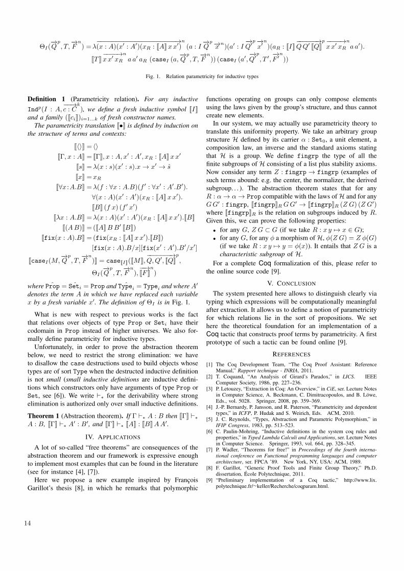
Fig. 1. Relation parametricity for inductive types
Definition 1 (Parametricity relation). For any inductive
Ind
p(I : A,��!c : C
k), we define a fresh inductive symbol JIK
and a family (JciK)i=1...k of fresh constructor names.
The parametricity translation J•K is defined by induction on
the structure of terms and contexts:
JhiK = hiJ�, x : AK = J�K, x : A, x
0 : A0, xR : JAKxx0
JsK =�(x : s)(x0 : s).x ! x
0 ! s
JxK =xR
J8x :A.BK =�(f : 8x : A.B)(f 0 : 8x0 : A0.B
0).
8(x : A)(x0 : A0)(xR : JAKxx0).
JBK (f x) (f 0x
0)
J�x : A.BK =�(x : A)(x0 : A0)(xR : JAKxx0).JBKJ(AB)K =(JAKBB
0 JBK)Jfix(x : A).BK =(fix(xR : JAKxx0).JBK)
[fix(x : A).B/x][fix(x0 : A0).B0/x
0]
JcaseI(M,
�!Q
p, T,
�!F
n)K = caseJIK(JMK,
�������!Q,Q
0, JQK
p,
⇥I(�!Q
p, T,
�!F
n),��!JF K
n)
where
ˆProp = ˆ
Seti = Prop and
ˆTypei = Typei and where A
0
denotes the term A in which we have replaced each variable
x by a fresh variable x
0. The definition of ⇥I is in Fig. 1.
What is new with respect to previous works is the factthat relations over objects of type Prop or Seti have theircodomain in Prop instead of higher universes. We also for-mally define parametricity for inductive types.
Unfortunately, in order to prove the abstraction theorembelow, we need to restrict the strong elimination: we haveto disallow the case destructions used to build objects whosetypes are of sort Type when the destructed inductive definitionis not small (small inductive definitions are inductive defini-tions which constructors only have arguments of type Prop orSet, see [6]). We write `⇤ for the derivability where strongelimination is authorized only over small inductive definitions.
Theorem 1 (Abstraction theorem). If � `⇤ A : B then J�K `⇤A : B, J�K `⇤ A
0 : B0, and J�K `⇤ JAK : JBKAA
0.
IV. APPLICATIONS
A lot of so-called “free theorems” are consequences of theabstraction theorem and our framework is expressive enoughto implement most examples that can be found in the literature(see for instance [4], [7]).
Here we propose a new example inspired by FrancoisGarillot’s thesis [8], in which he remarks that polymorphic
functions operating on groups can only compose elementsusing the laws given by the group’s structure, and thus cannotcreate new elements.
In our system, we may actually use parametricity theory totranslate this uniformity property. We take an arbitrary groupstructure H defined by its carrier ↵ : Set
0
, a unit element, acomposition law, an inverse and the standard axioms statingthat H is a group. We define fingrp the type of all thefinite subgroups of H consisting of a list plus stability axioms.Now consider any term Z : fingrp ! fingrp (examples ofsuch terms abound: e.g. the center, the normalizer, the derivedsubgroup. . . ). The abstraction theorem states that for anyR : ↵ ! ↵ ! Prop compatible with the laws of H and for anyGG
0 : fingrp, JfingrpKR GG
0 ! JfingrpKR (Z G) (Z G
0)where JfingrpKR is the relation on subgroups induced by R.Given this, we can prove the following properties:
• for any G, Z G ⇢ G (if we take R : x y 7! x 2 G);• for any G, for any � a morphism of H, �(Z G) = Z �(G)
(if we take R : x y 7! y = �(x)). It entails that Z G is acharacteristic subgroup of H.
For a complete Coq formalization of this, please refer tothe online source code [9].
V. CONCLUSION
The system presented here allows to distinguish clearly viatyping which expressions will be computationally meaningfulafter extraction. It allows us to define a notion of parametricityfor which relations lie in the sort of propositions. We sethere the theoretical foundation for an implementation of aCoq tactic that constructs proof terms by parametricity. A firstprototype of such a tactic can be found online [9].
REFERENCES
[1] The Coq Development Team, “The Coq Proof Assistant: ReferenceManual,” Rapport technique - INRIA, 2011.
[2] T. Coquand, “An Analysis of Girard’s Paradox,” in LICS. IEEEComputer Society, 1986, pp. 227–236.
[3] P. Letouzey, “Extraction in Coq: An Overview,” in CiE, ser. Lecture Notesin Computer Science, A. Beckmann, C. Dimitracopoulos, and B. Lowe,Eds., vol. 5028. Springer, 2008, pp. 359–369.
[4] J.-P. Bernardy, P. Jansson, and R. Paterson, “Parametricity and dependenttypes,” in ICFP, P. Hudak and S. Weirich, Eds. ACM, 2010.
[5] J. C. Reynolds, “Types, Abstraction and Parametric Polymorphism,” inIFIP Congress, 1983, pp. 513–523.
[6] C. Paulin-Mohring, “Inductive definitions in the system coq rules andproperties,” in Typed Lambda Calculi and Applications, ser. Lecture Notesin Computer Science. Springer, 1993, vol. 664, pp. 328–345.
[7] P. Wadler, “Theorems for free!” in Proceedings of the fourth interna-
tional conference on Functional programming languages and computer
architecture, ser. FPCA ’89. New York, NY, USA: ACM, 1989.[8] F. Garillot, “Generic Proof Tools and Finite Group Theory,” Ph.D.
dissertation, Ecole Polytechnique, 2011.[9] “Preliminary implementation of a Coq tactic,” http://www.lix.
polytechnique.fr/⇠keller/Recherche/coqparam.html.
15
Undecidable First-Order Theoriesof Affine Geometries
Antti KuusistoUniversity of [email protected]
Jeremy MeyersStanford University
Jonni VirtemaUniversity of [email protected]
I. INTRODUCTION
Tarski initiated a logic-based approach to formal geometrythat studies first-order structures with a ternary betweenness
relation (�) and a quaternary equidistance relation (⌘). Tarskiestablished, inter alia, that the first-order (FO) theory of(R2
,�,⌘) is decidable. For further information on the devel-opment of Tarski’s geometry, see [11]. Aiello and van Benthemconjectured in [1] that the FO-theory of the class of expansionsof (R2
,�) by unary predicates is decidable. We refute thisconjecture by showing that for all n � 2, the FO-theory ofthe class of monadic expansions of (Rn
,�) is ⇧11-hard and
therefore not even arithmetical. We also define a natural andcomprehensive class C of geometric structures (T,�), whereT ✓ Rn, and show that the for each structure (T,�) 2 C,the FO-theory of the class of monadic expansions of (T,�) isundecidable. We then consider classes of expansions of struc-tures (T,�) with restricted unary predicates, for example finitepredicates, and establish a variety of related undecidabilityresults. In addition to decidability questions, we briefly studythe expressivity of universal MSO and weak universal MSOover expansions of (Rn
,�). While the logics are incomparablein general, over expansions of (Rn
,�), formulae of weakuniversal MSO translate into equivalent formulae of universalMSO.
Our results could turn out intresting in investigations con-cerning logical aspects of spatial databases. It turns out thatthere is a canonical correspondence between (R2
,�) and(R, 0, 1, ·,+, <), see [7]. See the survey [9] for further detailson logical aspects of spatial databases.
The betweenness predicate is also studied in spatial logic[3]. The recent years have witnessed a significant increase inthe research on spatially motivated logics. Several interestingsystems with varying motivations have been investigated,see the surveys [2] and [4]. Our results contribute to theunderstanding of spatially motivated first-order languages, andhence they can be useful in the search for decidable (modal)spatial logics.
II. PRELIMINARIES
Tiling methods constitute a flexible framework for estab-lishing different degrees of undecidability of different kindsof problems. An input to a tiling problem is a finite set oftile types, i.e., a finite set of rectangles with coloured edges.The problem is to decide whether it is possible to tile a
predetermined region of space with tiles of the given type,under the constraint that adjacent edges of tiles have the samecolour. We make use of the three following variants of thetiling problem. The standard tiling problem asks whether aset T of tile types can tile the N⇥N grid, the recurrent tiling
problem asks whether T and some assigned tile type t 2 T cantile the N⇥N grid such that t occurs infinitely many times onthe leftmost column of the grid, and the torus tiling problem
asks if there exists some finite torus (i.e., a finite grid whoseborders wrap around to form a torus) such that the input setT tiles it.
Theorem II.1. The tiling problem is ⇧01-complete [5], the
recurrent tiling problem ⌃11-complete [8], and the periodic
tiling problem ⌃01-complete [6].
Let (Rn, d) be the n-dimensional Euclidean space with
the canonical metric d. We define the ternary Euclideanbetweenness relation � such that �(s, t, u) iff d(s, u) =d(s, t)+d(t, u). We study geometric betweenness structures ofthe type (T,�), where T ✓ Rn and where � is the restrictionof the betweenness predicate of Rn to the set T .
A subset S ✓ Rn is an m-dimensional flat of Rn, where0 m n, if there exists a set of m linearly independentvectors v1, . . . , vm 2 Rn and a vector h 2 Rn such that S isthe h-translated span of the vectors v1, . . . , vm, in other wordsS = {u 2 Rn | u = h+r1v1+ · · ·+rmvm, r1, . . . , rm 2 R}.Note that {(0, ...., 0)} is not considered to be a linearlyindependent set.
A set U ✓ Rn is a linearly regular m-dimensional flat,where 0 m n, if the following conditions hold.
1) There exists an m-dimensional flat S such that U ✓ S.2) There does not exist any (m � 1)-dimensional flat S
such that U ✓ S.3) U is linearly complete, i.e., if L ✓ U is a line in U and
L
0 ◆ L the corresponding line in Rn, and if r 2 L
0 isa point and ✏ 2 R+ a positive real number, then thereexists a point s 2 L such that d(s, r) < ✏. Here d is thecanonical metric of Rn.
4) U is linearly closed, i.e., if points x1, x2 2 U andx3, x4 2 U determine two lines that intersect in Rn,then the corresponding lines in U intersect in U .
A set T ✓ Rnextends linearly in mD, where m n, if
there exists a linearly regular m-dimensional flat S, a positivereal number ✏ 2 R+ and a point x 2 S \ T such that { u 2
16
S | d(x, u) < ✏ } ✓ T. It is easy show that for example therational plane Q2 and the closed rectangle [0, 1]⇥ [0, 1] ✓ R2
extend linearly in 2D.
III. RESULTS
While 8WMSO 6 MSO and 8MSO 6 WMSO in general,over models embedded in (Rn
,�), 8WMSO translates into8MSO and WMSO into MSO.
Theorem III.1 (Heine-Borel). A set S ✓ Rnis closed and
bounded iff every open cover of S has a finite subcover.
Theorem III.2. Let C be the class of expansions (Rn,�, P )
of (Rn,�) with a unary predicate P , and let F ✓ C be the
subclass of C where P is finite. The class F is first-order
definable with respect to C.
Proof: It follows directly from the Heine-Borel theoremthat a set T ✓ Rn is finite iff it is closed, bounded and consistsof isolated points of T . The proof of the current theorem relieson this fact. The argument is based on encoding topologicalinformation about open balls by first-order formulae. The ideais to replace open balls by open n-dimensional triangles.
We first define a formula parallel(x, y, u, v) stating inRn that the lines defined by x, y and u, v are parallel.With this formula we construct formulae basisk(x0, . . . , xk)and flatk(x0, . . . , xk, z) by simultaneous recursion. The for-mulae state roughly that vectors (x0, xi) form a basis ofan x0-centered k-dimensional flat, and that z is in theflat. With these formulae we recursively define formu-lae opentriangle(x0, . . . , xk, z) stating that z is in the k-dimensional open triangle defined by the points x0, . . . , xk.
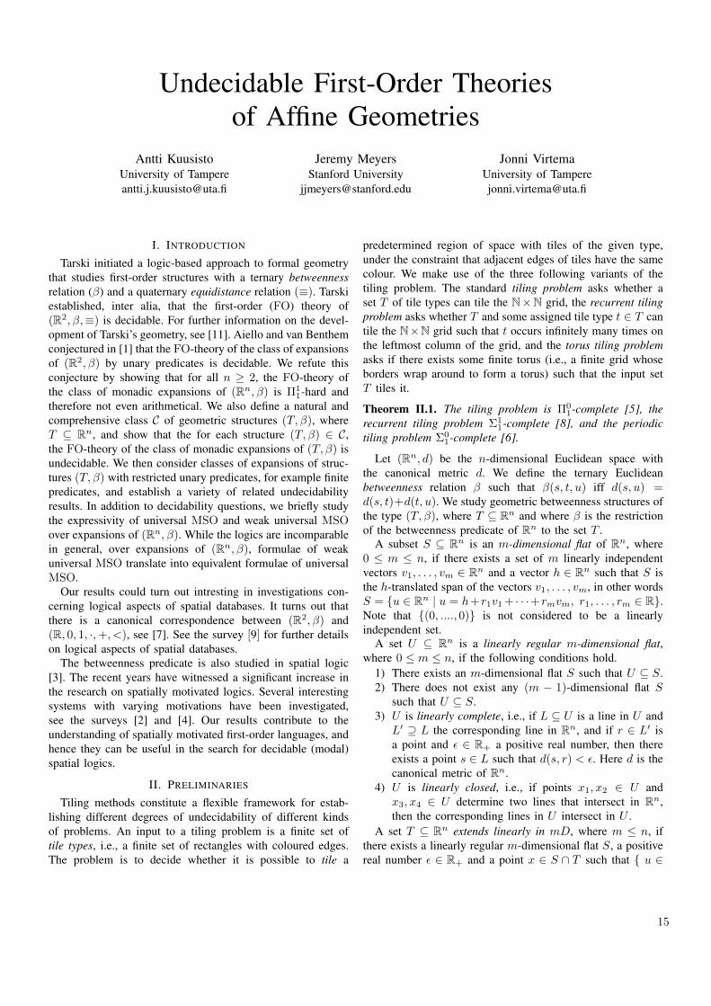
The first-order theory of the class of expansions (T,�, Pi2N)of any structure (T,�) that extends linearly in 2D is unde-cidable. Here Pi are monadic predicates. This is shown byinterpreting the N⇥N grid, or some superstructure of the grid,in the class of monadic expansions of (T,�). This is done bydefining two linear sequences of points that are stored in twopredicates P and Q. The sequences correspond to linear ordersthat begin by a prefix of the order type !. A superstructureof the grid is then interpreted by connecting the points ofthe linear sequence P to some upper bound of the sequenceQ, and vice versa. The grid points are the intersection pointsof the lines created in this fashion, see the Figure 1 for anillustration.
Theorem III.3. Let T ✓ Rnbe a set that extends linearly in
2D. The monadic ⇧11-theory of (T,�) is ⌃0
1-hard.
Extending linearly in 1D is not a sufficient condition forundecidability of the 8MSO-theory of (T,�). This can be seenfrom the fact that the 8MSO-theory of (Q, <) is decidable[10].
In Rn, it is possible to define predicates P and Q suchthat they correspond to linear sequences of the order type !
exactly. This enables the encoding of an isomorphic copy ofthe N ⇥ N grid in expansions of structures (Rn
,�), where
Fig. 1. Interpreting the grid in (T,�, P,Q).
n � 2. With an isomorphic copy of the grid, we can interpretthe recurring tiling problem in the structure created.
Theorem III.4. Let n � 2. The monadic ⇧11-theory of
the structure (Rn,�) is ⇧1
1-hard, and therefore not even
arithmetical.
When limiting attention to expansions of structures (T,�)with finite monadic predicates, we can use the periodic tilingproblem in order to establish undecidability of monadic ex-pansion classes of structures (T,�).
Theorem III.5. Let T ✓ Rnbe a set that extends linearly in
2D. The weak monadic ⇧11-theory of (T,�) is ⇧0
1-hard.
In addition to expansions with finite predicates, the periodictiling problem can be easily modified to yield undecidabilityof a wide variety of natural restricted monadic expansionsclasses of (R2
,�). These include expansions with predicatescorresponding to finite unions of closed rectangles, polygons,and other simple canonical classes of sets.
In the future we shall identify fragments of first-order logicthat lead to a decidable theory of the monadic expansion classof (R2
,�).
REFERENCES
[1] M. Aiello and J. van Benthem. A Modal Walk through Space. Journal
of Applied Non-Classical Logics 12(3-4):319-363, Hermes, 2002.[2] M. Aiello, I. Pratt-Hartmann, and J. van Benthem. What is Spatial Logic.
In [3].[3] M. Aiello, I. Pratt-Hartmann and J. van Benthem. Handbook of Spatial
Logics. Springer, 2007.[4] P. Balbiani, V. Goranko, R. Kellerman and D. Vakarelov. Logical
Theories for Fragments of Elementary Geometry. In [3].[5] R. Berger. The undecidability of the domino problem. Mem. Amer. Math.
Soc., 66, 1966.[6] Y. Gurevich and I. O. Koryakov. Remarks on Berger’s paper on the
domino problem. Siberian Mathematical Journal 13, 319-321, 1972.[7] M. Gyssens, J. Van den Bussche and D. Van Gucht. Complete Qeometric
Query Languages. J. Comput. System Sci. 58, 483-511, 1999.[8] D. Harel. Recurring Dominoes: Making the Highly Undecidable Highly
Understandable. Annals of Discrete Mathematics 24, 51-72, 1985.[9] B. Kujpers and J. Van den Bussche. Logical aspects of spatial database
theory. In Finite and Algorithmic Model Theory, Cambridge UniversityPress, 2011.
[10] M. O. Rabin. Decidability of second-order theories and automata oninfinite trees. Trans. of the Amer. Math. Soc. 141, 1-35, 1969.
[11] A. Tarski and S. Givant. Tarski’s System of Geometry. Bull. Symbolic
Logic 5(2), 1999.
17
Canonical Progress Measures for Parity GamesKonstantinos Mamouras
Department of Computer Science, Cornell University, Ithaca, NY, USAEmail: [email protected]
Abstract—A progress measure for a parity game is a labelings(·) of the vertices of the game that witnesses winning strategiesfor the players: Player 0 (Even) and Player 1 (Odd). We give anatural definition of a canonical progress measure for a paritygame G directly, without translating into the µ-calculus. Thelabel s(u) of a vertex u is defined to be the value of an infinitely-played game played on the graph of G.
In order to show the existence of these values, we introduce afinitely-played version of the game of duration at most n(n+1)/2moves, where n is the number of vertices. We show that the valuesfor the finitely-played version are the same as the values for theinfinitely-played version. This result also implies the existenceof optimal strategies for both players (in the infinitely-playedversion) that use memory of size O(nn(n+1)/2).
Without loss of generality we restrict attention to parity gamesin which Player 0 has a winning strategy from every vertex. Weshow that Player 0 has a memoryless strategy that ensures thecanonical progress measure everywhere. For Player 1, optimalstrategies are more complex. We consider the special case of 1-solitaire games, i.e. games where only Player 1 has non-trivialmoves. For 1-solitaire games, we show that Player 1 must havememory of size ⌦(n) in order to ensure the canonical progressmeasure. This lower bound extends, of course, to the generalcase. Moreover, for 1-solitaire games we show that Player 1 hasoptimal strategies that use memory of size O(n). For the generalcase, we do not have a matching upper bound for the size of thememory. We improve upon the upper bound previously stated:Player 1 has optimal strategies with memory of size O(nn).
Our results imply that the canonical progress measure for aparity game G records optimal strategies for Player 0. The samedoes not seem to be the case, however, for Player 1. We considerthis an indication that verifying canonical progress measures forparity games is not easier than finding them.
I. INTRODUCTION
A parity game involves two players, Player 0 (or Even)and Player 1 (or Odd). It is played on a directed graph whosevertices are labeled with natural numbers called priorities. Thevertices are partitioned into those that belong to Player 0 (0-vertices) and those that belong to Player 1 (1-vertices). A playstarts at some vertex where a token is placed. At every step,the player who owns the vertex with the token moves the tokento a successor vertex. Thus, an infinite sequence of vertices isformed. Player 0 wins the play if the maximum priority thatappears infinitely often is even, otherwise Player 1 wins.
Parity games are memorylessly determined, i.e. for everyvertex u some player � has a memoryless strategy f� s.t. everyplay that starts from u with Player � playing according to f� iswon by Player �. The winning region of Player 0 is the set ofvertices from which Player 0 has a winning strategy. Solvingparity games amounts to finding the winning region of Player0. By determinacy, the rest of the vertices are the winning
region of Player 1. The decision version of the problem is:Given a parity game G and a vertex u, does Player 0 havea winning strategy from u? Memoryless determinacy impliesthat the problem lies in NP\coNP [1]. Jurdzinski has shownthat the problem is even contained in UP \ coUP [2].
The importance of finding fast algorithms for solving paritygames lies in its polynomial-time equivalence to the problemof model checking the µ-calculus [3], [4]. Despite effortsof the community no polynomial-time algorithm is knownfor solving parity games. One line of research for designingalgorithms for parity games involves the notion of progressmeasure [5]. Progress measures, introduced by Klarlund andKozen in [6] where they are called Rabin measures, are annota-tions of graphs that record progress towards the satisfaction ofRabin conditions. Streett and Emerson used a similar notion,which they called signature [7], to study the µ-calculus.
A progress measure for a parity game is a labelling ofthe vertices of the game that witnesses winning strategies forthe players and hence also the winning regions. The progressmeasure records progress towards the satisfaction of the paritycondition. Walukiewicz considers canonical signature assign-ments for parity games [8], which are defined by translatingthe existence of a winning strategy into the µ-calculus and thenusing the notion of signature by Emerson and Streett [7]. Ourdefinition of the canonical progress measure for a parity gameis similar, but does not involve the µ-calculus. The canonicalprogress measure is unique and records winning strategiesfor the players that are “good” in the sense of minimizingthe progress measure. The progress measure is defined as alabelling s(·) of the vertices so that for a vertex u, s(u) isthe value of a game of infinite duration. This is well-defined,because s(u) is shown to be both the least outcome that Player0 can ensure and the greatest outcome that Player 1 can ensure.This result is also relevant to addressing a question raisedby Jurdzinski in [2]: Are canonical progress measures uniquesuccinct certificates for parity games? We do not resolve thisquestion here, but we believe that our results provide anindication for a negative answer.
We feel that studying canonical progress measures is im-portant in furthering our understanding of parity games. Thisis because finding the winning regions, winning strategies, aswell as finding some progress measure for a parity game are allequally hard problems. Finding the canonical progress measureis at least as hard. It amounts to finding “good” winningstrategies in a precise sense.
18
II. SUMMARY OF RESULTS
We define the outcome of an infinite play won by Player 0(Player 1) to be a function that maps each odd (even) priorityto a natural number. We call such a function a 0-signature
(1-signature). Consider the lexicographic ordering of thesefunctions, where larger priorities are more significant. Player0 wants to minimize the outcome and Player 1 to maximizeit. We show that for a vertex u both players have strategiesthat ensure the same outcome s(u) for plays starting from u.In order to show this, we consider a finitely-played version ofthe game of duration n(n+1)/2, where n is the number ofvertices. In the finitely-played version, a play ends as soon asa cycle is formed after the first occurrence of the maximumpriority that has appeared so far. We say that s(u) is the value
of u. The values for the finitely-played version are the sameas the values for the infinitely-played version. We show thisfact using a technique similar to the one used by Ehrenfeuchtand Mycielski in [9], where a similar result is established formean-payoff games. A corollary is that in the infinitely-playedversion the players have optimal strategies that use memory ofsize O(nn(n+1)/2). The canonical progress measure is definedto be the value assignment s(·).
Without loss of generality we study parity games in whichPlayer 0 has a winning strategy from every vertex. First, weestablish that Player 0 has a memoryless strategy f0 such thatfor every vertex u, f0 ensures outcome s(u) from u. Weshow an even stronger result: The canonical progress measurerecords all memoryless strategies that ensure the measure fromevery vertex.
We also study optimal strategies for Player 1. For thesimpler case of 1-solitaire games, i.e. games where only Player1 has non-trivial moves, we show that optimal strategies forPlayer 1 need memory of size at least ⌦(n). Moreover, optimalstrategies can be constructed that use memory of size at mostO(n). In order to construct optimal strategies we introducethe notions of extended outcome and extended value. Thesenotions formalize the idea that Player 1 tries to maximize theoutcome in as few steps as possible.
For general parity games, the linear lower bound for the sizeof the memory also applies. We do not have a matching upperbound. We improve, however, upon the O(nn(n+1)/2) upperbound we stated previously. We show that Player 1 has optimalstrategies that use memory of size at most O(nn). Again,constructing these optimal strategies involves the notions ofextended outcome and extended value.
III. CONCLUSION
Let G be a parity game and W0, W1 be the winningregions of Player 0 and 1 respectively. Our results for optimalstrategies (in general games) are summarized in the followingdiagram:
W0 W1
optimal 0-strategy: memoryless optimal 1-strategy: memoryless
optimal 1-strategy:⌦(n) |M | O(nn)
optimal 0-strategy:⌦(n) |M | O(nn)
We conjecture that there exist optimal 1-strategies for G[W0](and hence also optimal 0-strategies for G[W1]) with memoryof size at most O(n), where G[W ] denotes the restriction ofG to W .
The decision version of the problem of finding the canonicalprogress measure of a parity game is the following: Givena game G, a vertex u, and a 0-signature t, is it the casethat s(u) t? Call this problem CANONICAL. We havepreliminary results showing that if the above conjecture is true,then CANONICAL lies in NP \ coNP.
Let G be a game in which Player 0 wins from everyvertex. We have shown that the canonical progress measurerecords all possible memoryless 0-strategies that ensure themeasure. It does not seem, however, that we can read optimal1-strategies off from the measure. We take this as an indicationthat verifying canonical progress measures is not easier thanfinding them, since we might still need to guess an optimal1-strategy.
REFERENCES
[1] E. A. Emerson, C. S. Jutla, and A. P. Sistla, “On model-checking forfragments of µ-calculus,” in CAV’93, volume 697 of LNCS. Springer-Verlag, 1993, pp. 385–396.
[2] M. Jurdzinski, “Deciding the winner in parity games is in UP \ co-UP,”Information Processing Letters, vol. 68, pp. 119–124, 1998.
[3] D. Kozen, “Results on the propositional µ-calculus,” in Proceedings of the
9th Colloquium on Automata, Languages and Programming, ser. LectureNotes In Computer Science, vol. 140, 1982, pp. 348–359.
[4] ——, “Results on the propositional µ-calculus,” Theoretical Computer
Science, vol. 27, no. 3, pp. 333–354, 1983.[5] M. Jurdzinski, “Small progress measures for solving parity games,” in
Proceedings of the 17th Annual Symposium on Theoretical Aspects of
Computer Science, ser. STACS ’00. Springer-Verlag, 2000, pp. 290–301.
[6] N. Klarlund and D. Kozen, “Rabin measures and their applications tofairness and automata theory,” in Proceedings of Sixth Annual IEEE
Symposium on Logic in Computer Science (LICS 1991), 1991, pp. 256–265.
[7] R. S. Streett and E. A. Emerson, “An automata theoretic decision pro-cedure for the propositional mu-calculus,” Information and Computation,vol. 81, no. 3, pp. 249–264, 1989.
[8] I. Walukiewicz, “Pushdown processes: Games and model-checking,”Information and Computation, vol. 164, no. 2, pp. 234–263, 2001.
[9] A. Ehrenfeucht and J. Mycielski, “Positional strategies for mean payoffgames,” International Journal of Game Theory, vol. 8, pp. 109–113, 1979.
19
Down the Borel Hierarchy:Solving Muller Games via Safety Games⇤
Daniel Neider⇤, Roman Rabinovich†, and Martin Zimmermann⇤‡⇤ Lehrstuhl fur Informatik 7, RWTH Aachen University, Germany
Email: {neider, zimmermann}@automata.rwth-aachen.de† Mathematische Grundlagen der Informatik, RWTH Aachen University, Germany
Email: [email protected]‡ Institute of Informatics, University of Warsaw, Poland
Abstract—We transform a Muller game with n vertices into a
safety game with (n!)3 vertices whose solution allows to deter-
mine the winning regions of the Muller game and to compute a
finite-state winning strategy for one player. This yields a novel
memory structure and a natural notion of permissive strategies
for Muller games. Moreover, we generalize our construction by
presenting a new type of game reduction from infinite games to
safety games and show its applicability to several other winning
conditions.
I. INTRODUCTION
Muller games are a source of interesting and challengingquestions in the theory of infinite games. They are expressiveenough to describe all !-regular properties. Also, all winningconditions that depend only on the set of vertices visited in-finitely often can trivially be reduced to Muller games. Hence,they subsume Buchi, co-Buchi, parity, Rabin, and Streettconditions. Furthermore, Muller games are not positionallydetermined, i.e., both players need memory to implement theirwinning strategies. In this work, we present a framework todeal with three aspects of Muller games: solution algorithms,memory structures, and quality measures for strategies.
While investigating the interest of Muller games for “casualliving-room recreation” [1], McNaughton introduced scoringfunctions which describe the progress a player is makingtowards winning a play: consider a Muller game (A,F0,F1),where A is the arena and (F0,F1) is a partition of the setof loops in A used to determine the winner: Player i wins aplay ⇢ if the set of vertices visited infinitely often by ⇢ is inFi. The score of a set F of vertices measures how often Fhas been visited completely since the last visit of a vertex notin F . McNaughton proved the existence of strategies for thewinning player that bound her opponent’s scores by |A|! [1],provided the play starts in her winning region. Such a strategyis necessarily winning. The bound |A|! was subsequentlyimproved to 2 (and shown to be tight) [2]. Thus, the winner ofa Muller game can be determined by solving a (much simpler,albeit large) safety game. In the following, we present a novelalgorithm and a novel type of memory structure for Mullergames derived from solving this safety game. We also obtain
⇤This work was supported by the projects Games for Analysis and Synthesisof Interactive Computational Systems (GASICS) and Logic for Interaction(LINT) of the European Science Foundation.
a natural quality measure for strategies in Muller games andare able to extend the definition of permissiveness [3] fromparity games to Muller games.
In the following, we use the notions of winning strategiesand winning regions as defined in [4].
II. SCORING FUNCTIONS FOR MULLER GAMES
We begin by introducing scoring functions. For a moredetailed treatment we refer to [2], [1].
Definition 1. Let w 2 V ⇤, v 2 V , and ; 6= F ✓ V .• Define ScF (") = 0.• If v /2 F , then ScF (wv) = 0 and AccF (wv) = ;.• If v 2 F and AccF (w) = F \ {v}, then ScF (wv) =
ScF (w) + 1 and AccF (wv) = ;.• If v 2 F and AccF (w) 6= F \ {v}, then ScF (wv) =
ScF (w) and AccF (wv) = AccF (w) [ {v}.Now, let w,w0 2 V ⇤ and F ✓ 2V .
1) w is F-smaller than w0, denoted by w F w0, ifLast(w) = Last(w0) and for all F 2 F:
• ScF (w) < ScF (w0), or• ScF (w) = ScF (w0) and AccF (w) ✓ AccF (w0).
2) w and w0 are F-equivalent, denoted by w =F w0, ifw F w0 and w0 F w.
Our results rely on the following lemma.
Lemma 1 ([2]). In every Muller game G = (A,F0,F1),Player i has a winning strategy that bounds every ScF withF 2 F1�i by two during every consistent play.
Hence, a player wins the Muller game if and only if shecan prevent her opponent from ever reaching a score of three.This is a safety condition!
III. SOLVING MULLER BY SOLVING SAFETY
Fix a Muller game G = (A,F0,F1) and consider thefollowing safety game GS : the scores and accumulators ofPlayer 1 are tracked up to threshold three by the arena. Moreformally, we take the =F1 -quotient of the unraveling of A upto the positions where Player 1 reaches a score of three forthe first time. Player 1 wins a play in this (finite) arena, if hereaches a score of three. Hence, Player 0 wins if her opponentnever reaches a score of three.
20
Theorem 1. Let G be a Muller game with vertex set V . Onecan effectively construct a safety game GS with vertex set V S
and a mapping f : V ! V S with the following properties:1) For every v 2 V : Player i wins the Muller game from
v if and only if she wins the safety game from f(v).2) Player 0 has a finite-state winning strategy for G whose
set of memory states is V S .3) |V S | (|V |!)3.
Note that the first statement speaks about both players whilethe second one only speaks about Player 0. This is due tothe fact that the safety game keeps track of Player 1’s scoresonly. To obtain a winning strategy for Player 1, we have totrack Player 0’s scores. The first claim follows directly fromLemma 1 while the second one is proved by turning thewinning region of Player 0 in GS (restricted to the verticesreachable via a positional winning strategy for GS) into amemory structure whose strategy prevents Player 1 fromreaching a score of three in G. Such a strategy is winning.The size of this memory structure is at most cubically largerthen the size of the LAR memory structure.
Furthermore, by only using the F1 -maximal elements ofPlayer 0’s winning region as memory states, one obtains aneven smaller memory structure that still implements a winningstrategy. On the other hand, by using all vertices in the winningregion, but using the most general non-deterministic winningstrategy for Player 0 in GS (cf. [3]), we also obtain themost general non-deterministic winning strategy that preventsthe losing player from reaching a score of three (which canobviously be generalized to any threshold k). This extends thenotion of permissive strategies from parity to Muller games.
IV. SAFETY REDUCTIONS FOR INFINITE GAMES
Since Muller conditions are on a higher level of the Borelhierarchy than safety conditions, there is no game reductionfrom Muller to safety games (using the notion of reductionas defined, e.g., in [4]). Nonetheless, we have just solved aMuller game by solving a safety game. The price we have topay is that we only obtain a winning strategy for one playerwhile standard reductions yield winning strategies for both.Next, we present a general construction comprising our result.
Definition 2. A game G = (A,Win) with vertex set V andset Win ✓ V ! of winning plays for Player 0 is (finite-state)safety reducible, if there is a regular language L ✓ V ⇤ offinite words such that:
• For every play ⇢ 2 V !: if Pref(⇢) ✓ L, then ⇢ 2 Win.• If Player 0 wins from v, then she has a strategy � such
that Pref(⇢) ✓ L for every ⇢ consistent with � andstarting in v.
Note that a strategy � satisfying the second property is win-ning for Player 0 from v. Many solution algorithms for gamescan be phrased in this terminology, e.g., the progress measurealgorithms for parity games [5] respectively Rabin and Streettgames [6], as well as work on bounded synthesis [7] and LTLrealizability [8].
Theorem 2. Let G be a game with vertex set V that issafety reducible with language L(A) for some DFA A =(Q, V, q0, �, F ). Define the safety game G0 = (A⇥A, V ⇥F ).
1) For every v 2 V , Player 0 wins the G from v if and onlyif she wins G0 from (v, �(q0, v)).
2) Player 0 has a finite-state winning strategy for G withmemory states Q.
This results gives a unified approach to solving parity,Rabin, Streett, and Muller games (and many more) by solvingsafety games. Furthermore, the notion of safety-reduction al-lows to generalize permissiveness to all these games, yieldingwhat one could call L-permissiveness, i.e., we obtain the mostgeneral non-deterministic winning strategy that “stays” in L.
V. CONCLUSION
We have shown how to translate a Muller game into a safetygame to determine both winning regions and a finite-statewinning strategy for one player. Then, we generalized thisconstruction to a new type of reduction from infinite gamesto safety games with the same properties. The reduction fromMuller to safety games is implemented in the tool GAVS+1 [9].
The quality of a strategy can be measured by the maximalscore value the opponent can achieve. We conjecture that thereis no tradeoff between size and quality of a strategy.
Finally, there is a tight connection between permissivestrategies, progress measure algorithms, and safety reductionsfor parity games. Whether the safety reducibility of Mullergames can be turned into a progress measure algorithm issubject to ongoing research.
Acknowledgments. The authors want to thank WolfgangThomas for bringing McNaughton’s work to their attention,Wladimir Fridman for fruitful discussions, and Chih-HongCheng for his implementation of the algorithm.
REFERENCES
[1] R. McNaughton, “Playing infinite games in finite time,” in A Half-Centuryof Automata Theory, A. Salomaa, D. Wood, and S. Yu, Eds. WorldScientific, 2000, pp. 73–91.
[2] J. Fearnley and M. Zimmermann, “Playing Muller games in a hurry,” Int.J. Found. Comput. Sci., 2012, to appear.
[3] J. Bernet, D. Janin, and I. Walukiewicz, “Permissive strategies: fromparity games to safety games,” ITA, vol. 36, no. 3, pp. 261–275, 2002.
[4] E. Gradel, W. Thomas, and T. Wilke, Eds., Automata, Logics, and InfiniteGames: A Guide to Current Research, ser. LNCS, vol. 2500. Springer,2002.
[5] M. Jurdzinski, “Small progress measures for solving parity games,” inSTACS, ser. LNCS, H. Reichel and S. Tison, Eds., vol. 1770. Springer,2000, pp. 290–301.
[6] N. Piterman and A. Pnueli, “Faster solutions of Rabin and Streett games,”in LICS. IEEE Computer Society, 2006, pp. 275–284.
[7] S. Schewe and B. Finkbeiner, “Bounded synthesis,” in ATVA, ser. LNCS,K. S. Namjoshi, T. Yoneda, T. Higashino, and Y. Okamura, Eds., vol.4762. Springer, 2007, pp. 474–488.
[8] E. Filiot, N. Jin, and J.-F. Raskin, “Antichains and compositional algo-rithms for LTL synthesis,” Formal Methods in System Design, vol. 39,no. 3, pp. 261–296, 2011.
[9] C.-H. Cheng, A. Knoll, M. Luttenberger, and C. Buckl, “Gavs+: An openplatform for the research of algorithmic game solving,” in TACAS, ser.LNCS, P. A. Abdulla and K. R. M. Leino, Eds., vol. 6605. Springer,2011, pp. 258–261.
1See www6.in.tum.de/⇠chengch/gavs/ for details and to download the tool.
21
Interaction Graphs: AdditivesThomas Seiller
LAMA UMR 5127 CNRS — Université de SavoieBâtiment Chablais, Campus Scientifique73376 Le Bourget-du-Lac Cedex, France
Email: [email protected]
Abstract—Geometry of Interaction (GoI) is a kind of semanticsof linear logic proofs that aims at accounting for the dynamicalaspects of cut-elimination. We present here a parametrized con-struction of a Geometry of Interaction for Multiplicative AdditiveLinear Logic (MALL) in which proofs are represented by familiesof directed weighted graphs. This construction is founded on ageometrical identity between sets of cycles which generalizes thethree-term adjunctions which sustain usual GoI constructions.Contrarily to former Geometries of Interaction dealing withadditive connective, the proofs of MALL are interpreted by finiteobjects in this model. Moreover, we show how one can obtain, foreach value of the parameter, a denotational semantics for MALL.Finally, we show that two particular choices of the parameterrespectively give a combinatorial version of his latest GoI [1] or arefined version of older Geometries of Interaction [2], [3], [4]. Ourconstruction hence explains how Girard’s various constructionsrelate to each other by unveiling the unique geometrical identitysustaining them.
I. GEOMETRY OF INTERACTION
The Geometry of Interaction program [5] was introduced byGirard a couple of years after his discovery of Linear Logic[6]. It aims at giving a semantics of linear logic proofs thatwould account for the dynamical aspects of cut-elimination,hence of computation through the proofs-as-program corre-spondence. Informally, a GoI consists of:
• a set of mathematical objects — paraproofs — that willcontain, among other things, the interpretations of proofs(or �-terms);
• a notion of execution that will represent the dynamics ofcut-elimination (or �-reduction).
Then, from these basic notions, one should be able to "recon-struct" the logic from the way the paraproofs interact:
• From the notion of execution, one defines a notion oforthogonality between the paraproofs that will allow todefine formulas — types — as sets of paraproofs closedunder bi-orthogonality (a usual construction in realizabil-ity). The notion of orthogonality should be thought of asa way of defining negation based on its computationaleffect.
• The connectives on formulas are defined from "low-level"operations on the paraproofs, following the idea that therules governing the use of a connective should be definedby the way this connective acts at the level of proofs, i.e.by its computational effect.
Throughout the years, Girard defined several such seman-tics, mainly based on the interpretation of a proof as an opera-tor on an infinite-dimensional Hilbert space. It is worth noting
that the first version of GoI [2] allowed Abadi, Gonthier, andLevy [7] to explain the optimal reduction of �-calculus definedby Lamping [8].
The latest version of GoI [1], from which this work isgreatly inspired, is based on the interpretation of proofs asoperators in the type II1 hyperfinite factor. It is related to quan-tum coherent spaces [9], which suggest future applicationsto quantum computing. Moreover, the great generality andflexibility of the definition of exponentials also seem promisingwhen it comes to the study of complexity1.
II. INTERACTION GRAPHS
In a previous work [11], we developed a graph-theoreticalGoI for Multiplicative Linear Logic (MLL) where proofs areinterpreted by finite objects2. In this work [12] we show howthese graph-theoretical constructions can be generalized tofinite formal weighted sums of graphs, and how to constructadditive connectives in this setting. Contrarily to what happensin the two other versions of GoI dealing with additives [4],[1], proofs of MALL are interpreted in our framework by finiteobjects.
This construction is based on a geometrical identity —called the cyclic property — between sets of cycles whichis a generalization of GoI’s three-term adjunctions. As aconsequence of the cyclic property, one gets a three-term geo-metrical adjunction. From this geometrical adjunction and anyquantifying map from the interval ]0, 1] to R>0[{1}, one candefine a parametrized notion of orthogonality and construct ageometry of interaction for MALL. We are therefore able todefine not just one but a whole family of models, two of whichwill turn out to be combinatorial versions of Girard’s older [2],[3], [4] and more recent [1] GoI constructions.
We then proceed to show how, from any of these mod-els, one can obtain a ⇤-autonomous category GraphMLLwith` 6⇠= ⌦ and 1 6⇠= ?, i.e. a non-degenerate denotationalsemantics for MLL. As in all the versions of GoI dealingwith additive connectives, our construction of additives doesnot define a categorical product. However, it is possible todefine an internal notion of observational equivalence withinthe model. As a consequence of the cyclic property, wecan show that this notion of observational equivalence is a
1A first result in this direction was obtained by Girard [10] who obtaineda characterization of the class NL.
2Even though the graphs we consider can have an infinite set of edges,linear logic proofs are represented by finite graphs.
22
congruence on the category GraphMLL. We are then able todefine a categorical product from our additive connectiveswhen considering classes of observationally equivalent objects,obtaining a denotational semantics for MALL with additiveunits. This category is non-degenerate in the sense that noconnectives and units are equal and neither the mix rule northe weakening hold. This model is moreover obtained as a fullsubcategory of a ⇤-autonomous category, i.e. a model of MLLwith units.
Finally, we show how our framework is related to Girard’sversions of GoI. A first choice of quantifying map gives usa model that can be embedded in Girard’s GoI5 framework.It can be shown that it is a combinatorial version of (themultiplicative additive) fragment of GoI5. In particular, theorthogonality defined in our setting corresponds to Girard’snotion of orthogonality based on the Fuglede-Kadison determi-nant3. Our construction therefore gives insights on the notionof orthogonality used by Girard, and his use of idioms andpseudo-trace which both have a graph-theoretical counterpartin our construction.
We then proceed to show that a second choice of quan-tifying map defines a model where orthogonality is definedby nilpotency: our construction thus defines in this case a(refined) version of older Geometries of Interaction [2], [3],[4]. However, this choice of parameter yields a trivial modelof the additives. Nonetheless, the interaction graphs makea bridge between "old-style" geometry of interaction andGirard’s most recent work [1], unveiling in the process theunique geometrical identity — the so-called cyclic property— behind those seemingly different constructions.
3The Fuglede-Kadison determinant is a generalization of the determinantdefined in any type II1 factor [13].
REFERENCES
[1] J.-Y. Girard, “Geometry of interaction V: Logic in the hyperfinite factor.”Theoretical Computer Science, pp. 1860–1883, 2011.
[2] ——, “Geometry of interaction I: Interpretation of system f,” in In Proc.Logic Colloquium 88, 1989.
[3] ——, “Geometry of interaction II: Deadlock-free algorithms,” in Proc.of COLOG, LNCS 417. Springer, 1988.
[4] ——, “Geometry of interaction III: Accommodating the additives,” inAdvances in Linear Logic, LNS 222,CUP. Cambridge University Press,1995.
[5] ——, “Towards a geometry of interaction,” in Proc. of AMS Conferenceon Categories, Logic and Computer Science, 1989.
[6] ——, “Linear logic,” Theoretical Computer Science, vol. 50, pp. 1–102,1987.
[7] M. Abadi, G. Gonthier, and J.-J. Lévy, “The geometry of optimal lambdareduction,” in Proc. of the 19th Annual ACM Symposium on Principlesof Programming Languages. ACM Press, 1992.
[8] J. Lamping, “An algorithm for optimal lambda calculus reductions,” inProc. of the 17th Annual ACM Symposium on Principles of Program-ming Languages. San Francisco: ACM Press, 1990.
[9] J.-Y. Girard, “Between logic and quantic : a tract,” Institut de Mathé-matiques de Luminy, Octobre, Tech. Rep., 2003.
[10] ——, “Normativity in logic,” Epistemology vs. Ontology, 2011.[11] T. Seiller, “Interaction graphs: Multiplicatives,” to appear in Annals of
Pure and Applied Logic, 2011.[12] ——, “Interaction graphs: Additives,” preprint, 2012,
arXiv:1205.6557v1.[13] B. Fuglede and R. V. Kadison, “Determinant theory in finite factors,”
Annals of Mathematics, no. 2, p. 530, 1952.
23
Ribbon Proofs for Separation LogicJohn Wickerson
University of [email protected]
Mike DoddsUniversity of [email protected]
Matthew ParkinsonMicrosoft Research Cambridge
A program proof should not merely certify that a program iscorrect; it should explain why it is correct. A proof shouldbe more than ‘true’: it should be informative, and it shouldbe intelligible. Extending work by Bean [1], we introduce asystem that produces readable program proofs that are highlyscalable and easily modified.
The de facto standard for presenting program proofs inHoare logic [2] is the proof outline, in which the program’sinstructions are interspersed with ‘enough’ assertions to allowthe reader to reconstruct the derivation tree. As an example,Fig. 1a presents a proof outline for a program that performsin-place list reversal. A key asset of the proof outline iswhat we shall call instruction locality: that one can verifyeach instruction in isolation (by confirming that the assertionsimmediately above and below it form a valid Hoare triple) andimmediately deduce that the entire proof is correct.
The proof outline suffers several drawbacks, however. First,there is much repetition: ‘list ↵x’ appears redundantly in sixconsecutive assertions before it is used on line 25. Second,there is no distinction between those parts of an assertion thatare affected by an instruction and those that are merely in whatseparation logic calls the frame. For instance, line 19 affectsonly the second and fourth conjuncts of its preceding assertion,but it is difficult to deduce its effect because two unchangedconjuncts are interspersed. (Had we followed common practiceand reduced the size of the proof outline by combining thisline with the assignment on line 17, the effect would be evenharder to deduce.) Third, the use of logical variables is unclear.For instance, spotting that the � in line 20 differs from theone in line 22 requires careful examination, or else, as wehave done, an explicit textual comment. These minor problemsin our illustrative example quickly become devastating whenscaled to large programs.
Separation logic [3], [4] provides a mechanism for handlinga second dimension of locality: resource locality. One can useseparation logic’s small axioms to reason about an instructionoperating only on the resources (i.e. memory cells) that itneeds, and immediately deduce its effect on the entire state us-ing the frame rule. To depict this mechanism in a proof outline,one must show applications of the frame rule explicitly. Butthis is tedious; moreover, it is difficult to know when and whatto frame. Meanwhile, the ribbon proof inherently supportsresource locality. Its primitive steps correspond exactly to thesmall axioms. It is thus an ideal representation for exploitingboth forms of locality that separation logic provides.
Figure 1b recasts our proof as a ribbon proof. The state is
distributed across several ribbons (thick borders). Horizontallyseparated ribbons describe disjoint parts of the state. Theinstructions are in grey bars, and the scope of each logicalvariable is delimited by an existential box (thin borders).We are free to stretch ribbons as required by the layout,and, because ⇤ is commutative, we can ‘twist’ them too. Atemporarily inactive ribbon slides discreetly down the sideof the proof. This effect is achieved by invoking the framerule at each instruction; but crucially in a ribbon proof, theseinvocations are implicit and do not increase the diagram’scomplexity. Observe that the repetition has disappeared, andthat each instruction’s effect is clear: it affects exactly thoseassertions directly above and below it, while framed assertions(which must not mention variables written by the instruction)bypass to the left or right. Existential boxes extend verticallyto indicate the range of steps over which the same witness isused, thus making the usage of logical variables visually clear.
In our full paper [5]:• we present an Isabelle-checked graph-based formalisation
of our proof system;• we showcase, with a ribbon proof of the memory manager
from Version 7 Unix, the ability of our diagrams topresent readable proofs of large, complex programs; and
• we describe a prototype tool for mechanically checkingribbon proofs in Isabelle. Provided with a small proofscript for each primitive step, our tool assembles a scriptthat verifies the entire diagram. The tool handles tediumssuch as the associativity and commutativity of ⇤ automat-ically, leaving the user to concentrate on the interestingparts of the proof.
This work lays the foundations for a new way to use logic tounderstand programs. Where a proof outline essentially flattensa proof to a list of assertions, our system produces geometricobjects that illuminate the structure of proofs, and which canbe navigated, modified and simplified by leveraging humanvisual intuition.
REFERENCES
[1] J. Bean, “Ribbon proofs,” in MFPS, 2003.[2] C. Hoare, “An axiomatic basis for computer programming,” Communica-
tions of the ACM, vol. 12, no. 10, October 1969.[3] J. C. Reynolds, “Separation logic: A logic for shared mutable data
structures,” in LICS, 2002.[4] S. Ishtiaq and P. W. O’Hearn, “BI as an assertion language for mutable
data structures,” in POPL, 2001.[5] J. Wickerson, M. Dodds, and M. J. Parkinson, “Ribbon proofs for sepa-
ration logic,” May 2012, http://www.cl.cam.ac.uk/~jpw48/ribbons.html.
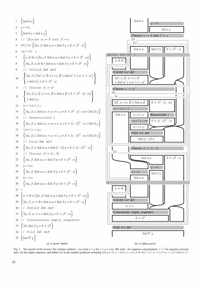
24
1n
list � xo
2 y:=0;
3n
list � x ⇤ list ✏yo
4 // Choose ↵ := � and � := ✏
5 while
n
9↵,�. list ↵x ⇤ list � y ⇤ � .= �† · ↵
o
6 (x!=0) {
7n
x
˙6= 0 ⇤ (9↵,�. list ↵x ⇤ list � y ⇤ � .= �† · ↵)
o
8n
9↵,�.x ˙6= 0 ⇤ list ↵x ⇤ list � y ⇤ � .= �† · ↵
o
9 // Unfold list def
10
8
<
:
9↵,�. (9↵0, i, Z.x 7! i, Z ⇤ list ↵0z ⇤ ↵ .
= i · ↵0)
⇤ list � y ⇤ � .= �† · ↵
9
=
;
11 // Choose ↵ := ↵0
12
8
<
:
9↵,�, i, Z.x 7! i, Z ⇤ list ↵Z ⇤ � .= �† · (i · ↵)
⇤ list � y
9
=
;
13 z:=[x+1];
14n
9↵,�, i. list ↵z ⇤ x 7! i,z ⇤ � .= �† · (i · ↵) ⇤ list � y
o
15 // Reassociate i
16n
9↵,�, i. list ↵z ⇤ x 7! i,z ⇤ � .= (i · �)† · ↵ ⇤ list � y
o
17 [x+1]:=y;
18n
9↵,�, i. list ↵z ⇤ x 7! i,y ⇤ � .= (i · �)† · ↵ ⇤ list � y
o
19 // Fold list def
20n
9↵,�, i. list ↵z ⇤ list (i · �)x ⇤ � .= (i · �)† · ↵
o
21 // Choose � := (i · �)22
n
9↵,�. list ↵z ⇤ list � x ⇤ � .= �† · ↵
o
23 y:=x;
24n
9↵,�. list ↵z ⇤ list � y ⇤ � .= �† · ↵
o
25 x:=z;
26n
9↵,�. list ↵x ⇤ list � y ⇤ � .= �† · ↵
o
27 }
28n
x
.= 0 ⇤ (9↵,�. list ↵x ⇤ list � y ⇤ � .
= �† · ↵)o
29n
9↵,�.x .= 0 ⇤ list ↵x ⇤ list � y ⇤ � .
= �† · ↵o
30 // Unfold list def
31n
9↵,�.↵ .= ✏ ⇤ list � y ⇤ � .
= �† · ↵o
32 // Concatenate empty sequence
33n
9�. list � y ⇤ � .= �†
o
34 // Fold list def
35n
list �† yo
(a) A proof outline
while (x!=0) {
}
list � xy:=0
list ✏y
Choose ↵ := � and � := ✏9↵9�
list ↵x list � y �.= �† · ↵
x
˙6= 0
Unfold list def
9↵0, i, Z.x 7! i, Z⇤ list ↵0 z ⇤ ↵ .
= i · ↵0
Choose ↵ := ↵0
9↵9i
9Z.x 7! i, Z ⇤ list ↵Z �.= �† · (i · ↵)
z:=[x+1]
list ↵z x 7! i,z Reassociate i
�.= (i · �)† · ↵
[x+1]:=y
x 7! i,y
Fold list def
list (i · �)x
Choose � := (i · �)9�
list � x �.= �† · ↵
y:=x
x:=z list � y
list ↵x
x
.= 0
Unfold list def
↵.= ✏
Concatenate empty sequence
�.= �†
Fold list def
list �† y
(b) A ribbon proof
Fig. 1. Two proofs of list reverse. For a binary relation r, we write x r y for x r y^emp. We write · for sequence concatenation, (�)† for sequence reversaland ✏ for the empty sequence, and define list as the smallest predicate satisfying list ↵x , x
.
= 0⇤↵ .
= ✏_x
˙6= 0⇤9↵0, i, x
0. x 7! i, x
0⇤↵ .
= i·↵0⇤list ↵0x
0.
Short Papers from the Specific Short Papers Call
25

26

27
Logical Bell InequalitiesSamson Abramsky
Department of Computer Science, University of OxfordWolfson Building, Parks Road, Oxford, U.K.
Lucien HardyPerimeter Institute, 31 Caroline Street North
Waterloo, ON N2L 2Y5, [email protected]
Bell inequalities [3], [4] play a fundamental role in quantuminformation and computation and the foundations of quantummechanics. They provide the basis for experimental demon-strations of non-locality and entanglement as fundamentalnon-classical resources for information processing. There isa huge literature on Bell inequalities, with many ingeniousderivations of families of inequalities. However, a unifyingprinciple with a clear conceptual basis has proved elusive.In [2], we introduce a form of Bell inequality based onlogical consistency conditions, which we call logical Bellinequalities. This approach is both conceptually illuminatingand technically powerful. We show that a rational inequalityis satisfied by all non-contextual models if and only if itis equivalent to a logical Bell inequality. Thus quantitativetests for contextuality or non-locality always hinge on purelylogical consistency conditions. We obtain explicit descriptionsof complete sets of inequalities for the convex polytope ofnon-contextual probability models, and the derived polytopeof expectation values for these models. Moreover, these resultsare obtained at a high level of generality; they apply notonly to the familiar cases of Bell-type scenarios, for anynumber of parties, but to all Kochen-Specker configurations,and in fact to any family of sets of compatible measurements.This generality is achieved by working with measurementcovers, following the sheaf-theoretic approach to non-localityand contextuality introduced by the first author and AdamBrandenburger in [1].
We also obtain results for a number of special cases. Weshow that a model achieves maximal violation of a logicalBell inequality if and only if it is strongly (or maximally)contextual. We show that all Kochen-Specker configurationslead to maximal violations of logical Bell inequalities in astate-independent fashion. We also derive specific violationsof logical Bell inequalities for models which are possibilis-tically contextual, meaning that they admit logical proofs ofcontextuality. Well-known examples of such models are thosearising from the construction in [6].
Inspiration for the present work was drawn from [5], whichderives some particular cases of logical Bell inequalities.Developing these ideas in the general setting provided by [1]proves to be fruitful, and indicates the potential for a structuralapproach to quantum foundations, using tools developed in thesemantics of computation.
We believe that the logical perspective opened up on Bellinequalities in this work, in a very general setting, will be
accessible and interesting to computer scientists working inlogical foundations of information and computation.
We shall illustrate the ideas by showing how the essentialpoint can be conveyed in a very simple setting, withoutpresupposing quantum mechanics or any other specific theory.
A. A Simple Observation
We begin with a simple and very general scenario.Suppose we have propositional formulas '1, . . . ,'N . We
suppose further that we can assign a probability pi to each'i.
In particular, we have in the mind the situation wherethe boolean variables appearing in 'i correspond to empir-ically testable quantities; 'i then expresses a condition onthe outcomes of an experiment involving these quantities.The probabilities pi are obtained from the statistics of theseexperiments.
Now let P be the probability of � :=V
i 'i. Usingelementary probability theory, we can calculate:
1� P = Prob(¬�) = Prob(_
i
¬'i)
X
i
Prob(¬'i) =X
i
(1� pi) = N �X
i
pi.
Tidying this up yieldsP
i pi N � 1 + P .Now suppose that the formulas 'i are jointly contradictory;
i.e. � is unsatisfiable. This implies that P = 0. Hence weobtain the inequality
X
i
pi N � 1.
This is an example of a logical Bell inequality. This basic formis generalized in [2] using a notion of K-consistency, relatedto the well-known MAX-SAT problem in computationalcomplexity [7].
B. A Curious Observation
Quantum Mechanics tells us that we can find propositions'i describing outcomes of certain measurements, which notonly can but have been performed. From the observed statisticsof these experiments, we have very highly confirmed proba-bilities pi. These propositions are easily seen to be jointlycontradictory. Nevertheless, the inequality
X
i
pi N � 1
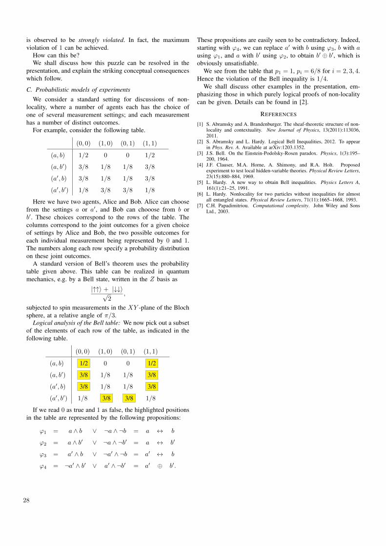
28
is observed to be strongly violated. In fact, the maximumviolation of 1 can be achieved.
How can this be?We shall discuss how this puzzle can be resolved in the
presentation, and explain the striking conceptual consequenceswhich follow.
C. Probabilistic models of experimentsWe consider a standard setting for discussions of non-
locality, where a number of agents each has the choice ofone of several measurement settings; and each measurementhas a number of distinct outcomes.
For example, consider the following table.
(0, 0) (1, 0) (0, 1) (1, 1)
(a, b) 1/2 0 0 1/2
(a, b0) 3/8 1/8 1/8 3/8
(a0, b) 3/8 1/8 1/8 3/8
(a0, b0) 1/8 3/8 3/8 1/8
Here we have two agents, Alice and Bob. Alice can choosefrom the settings a or a0, and Bob can chooose from b orb0. These choices correspond to the rows of the table. Thecolumns correspond to the joint outcomes for a given choiceof settings by Alice and Bob, the two possible outcomes foreach individual measurement being represented by 0 and 1.The numbers along each row specify a probability distributionon these joint outcomes.
A standard version of Bell’s theorem uses the probabilitytable given above. This table can be realized in quantummechanics, e.g. by a Bell state, written in the Z basis as
|""i + |##ip2
,
subjected to spin measurements in the XY -plane of the Blochsphere, at a relative angle of ⇡/3.
Logical analysis of the Bell table: We now pick out a subsetof the elements of each row of the table, as indicated in thefollowing table.
(0, 0) (1, 0) (0, 1) (1, 1)
(a, b) 1/2 0 0 1/2
(a, b0) 3/8 1/8 1/8 3/8
(a0, b) 3/8 1/8 1/8 3/8
(a0, b0) 1/8 3/8 3/8 1/8
If we read 0 as true and 1 as false, the highlighted positionsin the table are represented by the following propositions:
'1 = a ^ b _ ¬a ^ ¬b = a $ b
'2 = a ^ b0 _ ¬a ^ ¬b0 = a $ b0
'3 = a0 ^ b _ ¬a0 ^ ¬b = a0 $ b
'4 = ¬a0 ^ b0 _ a0 ^ ¬b0 = a0 � b0.
These propositions are easily seen to be contradictory. Indeed,starting with '4, we can replace a0 with b using '3, b with ausing '1, and a with b0 using '2, to obtain b0 � b0, which isobviously unsatisfiable.
We see from the table that p1 = 1, pi = 6/8 for i = 2, 3, 4.Hence the violation of the Bell inequality is 1/4.
We shall discuss other examples in the presentation, em-phasizing those in which purely logical proofs of non-localitycan be given. Details can be found in [2].
REFERENCES
[1] S. Abramsky and A. Brandenburger. The sheaf-theoretic structure of non-locality and contextuality. New Journal of Physics, 13(2011):113036,2011.
[2] S. Abramsky and L. Hardy. Logical Bell Inequalities, 2012. To appearin Phys. Rev. A. Available at arXiv:1203.1352.
[3] J.S. Bell. On the Einstein-Podolsky-Rosen paradox. Physics, 1(3):195–200, 1964.
[4] J.F. Clauser, M.A. Horne, A. Shimony, and R.A. Holt. Proposedexperiment to test local hidden-variable theories. Physical Review Letters,23(15):880–884, 1969.
[5] L. Hardy. A new way to obtain Bell inequalities. Physics Letters A,161(1):21–25, 1991.
[6] L. Hardy. Nonlocality for two particles without inequalities for almostall entangled states. Physical Review Letters, 71(11):1665–1668, 1993.
[7] C.H. Papadimitriou. Computational complexity. John Wiley and SonsLtd., 2003.
29
Approximations of Conjunctive QueriesPablo Barcelo
Department of Computer ScienceUniversity of ChileSantiago, Chile
Leonid LibkinSchool of InformaticsUniversity of Edinburgh
Edinburgh, [email protected]
Miguel RomeroDepartment of Computer Science
University of ChileSantiago, Chile
Abstract—The term conjunctive queries refers to the ∃,∧-fragment of first-order predicate logic. These are the most com-mon queries used in relational database systems as they capturethe operations of selection, projection, and join of relationalalgebra. While data complexity of these queries is very low,combined complexity is well-known to be NP-complete. Giventhe importance of conjunctive queries, subclasses guaranteeingtractable combined complexity have been extensively studied;those include classes of acyclic queries, as well as queries ofbounded treewidth and bounded hypertree width.We have recently initiated a study of approximations of
conjunctive queries from the static analysis point of view. The keyidea is to approximate “bad” (intractable) conjunctive queriesby ones from “good” (tractable) classes. The paper appears atPODS’2012 and combines logical techniques with those fromgraph theory, especially theory of graph homomorphisms. Webelieve a brief account of this work could be of interest to theLICS community. Specifically, in PODS’12 paper we showed thatapproximations exist for the above classes of tractable conjunctivequeries, that their sizes are at most polynomial in the sizes ofthe queries that are approximated, and that approximations canbe found in single-exponential time.
I. INTRODUCTION
The concept of approximating queries by those that areeasier to execute is very common in database research [10]. Wehave recently initiated a study of approximations of conjunc-tive queries [2]. These queries, which form the ∃,∧-fragmentof first-order logic, play a special role in database applications[1]. In addition, we have a very good understanding oftheir complexity. While in general their combined complexityis NP-complete [3], tractable classes of conjunctive querieshave been identified; these include acyclic queries, queries ofbounded treewidth, and queries of bounded hypertree width,see [5], [6], [7], [9], [11]. We studied approximations fromthe point of view of static analysis, i.e., we looked forapproximations independent of the input database: for a queryQ, we want to find another query Q′ that will be much fasterthan Q, and whose output would be close to the output of Qon all databases.We have shown in [2] that approximations always exist for
classes mentioned above; furthermore, sizes of approximationsare at most polynomial in the size of the original query (andoften they do not exceed the size of the original query), andthey can be found in at most single-exponential time.To see why these properties are desirable, consider, for
instance, the complexity of checking whether a tuple a belongs
to the output of a conjunctive query Q on a database D.This is of the order |D|O(|Q|), where | · | measures the sizeof a database or a query [1]; the problem is actually knownto be NP-complete [3]. The data complexity of conjunctivequery evaluation is of course very low (in AC0), but if we areconcerned with evaluating queries over large data sets, havingO(|Q|) as the exponent may be too high. With conjunctivequeries from the good classes mentioned above, the O(|Q|)exponent is replaced by a fixed one. For instance, for acyclicconjunctive queries, evaluation can be done in time O(|D|·|Q|)[11]. Thus, assuming that we can find an approximationrelatively fast (for instance, in time 2O(|Q| log |Q|)) and its sizeis roughly bounded by the size of Q, we may want to checkif the approximation gives us the answer first. The complexityof doing so is 2O(|Q| log |Q|) + O(|D| · |Q|), which is likelyto be much less than |D|O(|Q|) on very large databases D.
II. DEFINITION OF APPROXIMATIONS
Suppose we have a query, i.e., a (∃,∧)-FO formula Q(x),and we want to approximate it by Q′(x) coming from a goodclass of queries C. There are two requirements for this:1) Q′ should not return false results, i.e., Q′ ⊆ Q (that is,
Q′(D) ⊆ Q(D) for all databases D);2) we cannot find a better approximating query, i.e., thereis no Q′′ ∈ C satisfying Q′ ! Q′′ ⊆ Q.
Such a query Q′, if it exists, is called a C-approximation ofQ.The classes we consider are divided into graph-based and
hypergraph-based classes. Both are obtained from the syntaxof the query. Given a query Q, we define its graph G(Q) andits hypergraph H(Q) as graphs of hypergraphs whose nodesare variables in Q. In G(Q), there is an edge between x andy if they occur in the same atomic subformula. In H(Q),each atomic subformula over variables x1, . . . , xm generatesa hyperedge {x1, . . . , xm}. Now the classes are:
• Hypergraph-based classes: these are classes HTW(k) ofqueries Q such that hypertree width (see [6]) of H(Q) isat most k. The class HTW(1) is also known as the classof acyclic queries.
• Graph-based classes: these are classes TW(k) of queriesQ such such that the treewidth of G(Q) is at most k.
As already mentioned, these are the standard tractable classesof conjunctive queries. Graph- and hypergraph-based notionsare in general incompatible [4].
30
The notion of approximations can be reformulated in termsof homomorphisms of graphs (and relational structures), con-necting it with many concepts studied in the field of constraintsatisfaction. Since Q ⊆ Q′ iff there is a homomorphismTQ′ → TQ from the tableau TQ′ of Q′ to the tableau TQ ofQ, finding an approximation in class C amounts to finding thelargest elements of C below a given structure in the lattice ofstructures and homomorphisms [8]. In fact we use techniquesof [8] extensively in our proofs.
III. SUMMARY OF RESULTS
A. Graph-based notions
Let C be a class of graphs closed under taking subgraphs.Assume that a single-element loop is in C (it has treewidth 1and is harmless). Slightly abusing notation, we also use C todenote the class of queries Q with G(Q) ∈ C.We show the following:1) every conjunctive query has a C-approximation;2) each approximation is equivalent to one that has at mostas many atomic subformulae as Q (i.e., at most as manysubgoals as Q);
3) an approximation can be constructed in time2O(|Q| log |Q|);
4) there are at most exponentially many non-equivalentapproximations of Q (and the exponential number ofapproximations can be witnessed).
We also study the complexity of the problem of recognizingapproximations: given Q and Q′, check whether Q′ is a C-approximation of Q. We show that when C = TW(k), fork ≥ 1, this problem is DP-complete. This holds even if Q, Q′
are minimized, i.e., their tableaux are cores.We then look what happens when we ask queries over
graphs, i.e., the vocabulary of a single binary relation E(·, ·).We show (for Boolean queries), the following trichotomy.If G(Q) is not bipartite, then only a trivial approxima-tion ∃x E(x, x) exists. If G(Q) is bipartite and has anunbalanced directed cycle (with a different number of for-ward and backward edges), then the only approximation is∃x, y E(x, y)∧E(y, x) (which is essentially trivial since everyquery with a bipartite graph contains this query). But if G(Q)is bipartite and has no unbalanced cycles, thenQ has nontrivialapproximations with strictly fewer subgoals than Q itself.While the condition above may seem restrictive, it only
applies to queries over graphs; with higher arities it is easierto get nontrivial approximation (we show an example later).
B. Hypergraph-based notions
For hypergraph-based classes, we need a more complexclosure condition for the existence of approximations if wewant to capture classes such as HTW(k). Specifically, werequire that hypergraphs be closed under two operations:
• restriction to induced subhypergraphs;• extensions of hyperedges with fresh nodes (not used inother hyperedges).
We prove that each class HTW(k) satisfies these conditions.Then, we show that exactly the same existence results as thosementioned in the graph-based subsection hold. Hence, we getapproximations for all the classes of conjunctive queries thatadmit tractable evaluation.
IV. A COUPLE OF EXAMPLES
We start with the simplest case, Boolean queriesover graphs, and write then in the standard rule-based notation for conjunctive queries. Consider aquery Q1:–E(x, y), E(y, z), E(z, x). Its graph is notbipartite and its best acyclic approximation is trivial:Q′
1:–E(x, x). Let Pm(x0, . . . , xm) be the conjunctivequery stating that x0, . . . , xm form a path of length m,i.e., E(x0, x1), . . . , E(xm−1, xm). If we now look atQ2 :– P3(x, y, z, u), P3(x′, y′, z′, u′), E(x, z′), E(y, u′)(which has a cycle with variables x, y, z′, u′), thenQ′
2:–P4(x, y, z, u, v) is its nontrivial acyclic approximation.Note that the tableau of Q2 is bipartite.With higher arities, we get richer approximations
within both graph-based and hypergraph-based classes.Consider, for instance, a query over ternary relations:Q3 :– R(x, y, z), R(y, x, u), R(u, z, x). This is a slightextension of the bad query Q1 (just remove syntacticallyx and you get a 3-cycle). But it has nontrivial TW(1)-approximations (the best for graph-based classes), e.g.,Q′
3 :– R(x, y, y), R(y, x, y), R(y, y, x).As another example, consider a query
Q4 :– R(x, y, z), R(z, u, v), R(v, w, x).
If we had a binary relation instead and omitted the middleattribute, we again would obtain a query whose tableau isa 3-cycle, thus having only trivial approximations. However,going beyond graphs lets us find nontrivial hypergraph-based(particularly, acyclic) approximations. In fact this query hasseveral non-equivalent acyclic approximations, for instanceQ′
4 :– R(x, y, z), R(z, u, y), R(y, v, x).
REFERENCES[1] S. Abiteboul, R. Hull, and V. Vianu. Foundations of Databases.
Addison-Wesley, 1995.[2] P. Barcelo, L. Libkin, M. Romero. Efficient approximations of conjunc-
tive queries. In PODS’12.[3] A. Chandra and P. Merlin. Optimal implementation of conjunctive
queries in relational data bases. In STOC’77, pages 77–90.[4] J. Flum, M. Frick, and M. Grohe. Query evaluation via tree-
decompositions. J. ACM, 49 (2002), 716–752.[5] G. Gottlob, N. Leone, and F. Scarcello. The complexity of acyclic
conjunctive queries. J. ACM, 48 (2001), 431–498.[6] G. Gottlob, N. Leone, and F. Scarcello. Hypertree decompositions and
tractable queries. JCSS, 64 (2002), 579–627.[7] M. Grohe, T. Schwentick, and L. Segoufin. When is the evaluation of
conjunctive queries tractable? In STOC’01, pages 657–666.[8] P. Hell and J. Nesetril. Graphs and Homomorphisms. Oxford University
Press, 2004.[9] P. Kolaitis and M. Vardi. Conjunctive-query containment and constraint
satisfaction. JCSS 61(2):302-332 (2000).[10] Q. Liu. Approximate query processing. Encyclopedia of Database
Systems, 2009, pages 113–119.[11] M. Yannakakis. Algorithms for acyclic database schemes. In Proc. Conf.
on Very Large Databases, 1981, pages 82–94.
31
Complete Axiomatizations of Fragments ofMonadic Second-Order Logic on Finite Trees
Amelie GheerbrantSchool of Informatics
University of EdinburghEdinburgh, UK
Email: [email protected]
Balder ten CateDepartment of Computer Science
University of California Santa CruzSanta Cruz, USA
Email: [email protected]
Abstract—We present a general model-theoretic techniquethat we developed and used in [3], [4] to obtain completeaxiomatizations of fragments of MSO on finite trees. There ismuch interest in studying logics on finite trees, and many logicsof interest are fragments of MSO. Previously FO axiomatizationswere known. To produce axiomatizations beyond FO, we hadto develop a new technique that combines classical tools frominfinite model theory (Henkin semantics for higher-order logics)with those more typical in finite model theory (Ehrenfeucht-Fraısse games, and their composition). The key idea behind thetechnique is to analyze infinite Henkin models of our axioms,and use games to show that they are elementarily equivalent tofinite trees.
Given the general interest in the LICS community in logics onfinite trees, and a new set of tools developed by us (that combineclassical and finite model theory), we believe that a brief accountof this work will be of interest to the LICS audience.
I. INTRODUCTION
Recently there has been much interest in studying logicsover ordered unranked trees, mainly due to connections withXML research, since labeled unranked trees serve as a standardabstraction of XML documents. Logics are used to describe thestructure of XML documents, and to query data they contain,and absolute majority of those used in this context happen tobe fragments of MSO (see [8]).
The goal of this work is to obtain complete axiomatizationsof MSO and its fragments on finite node-labeled sibling-ordered trees. Such axiomatizations have previously beenpresented for FO-theories [5] but extending the work toMSO presents a number of challenges. We address thoseby developing a new model-theoretic technique by which weobtain complete axiomatizations not only of MSO but also ofsome of its fragments, such as monadic transitive closure logicand monadic least fixed-point logic.
The new tools we developed combine traditional model-theoretic techniques used to show completeness, with tech-niques more common in finite model theory, namelyEhrenfeucht-Fraısse games as well as techniques for compos-ing games. These results have not been presented in the forumstraditionally attended by LICS attendees: the conference ver-sion appeared in [3] (the journal version is to appear in [4]).As this work addresses traditional LICS topics via using a newset of techniques, we believe that the LICS community couldbe interested in a short presentation of this work.
To give a flavor of our results and techniques, below wedescribe the approach for MSO. We give a brief account of thekey ingredients: Henkin completeness and Feferman-Vaughttheorems, that we need to obtain our results. References [3],[4] can be consulted for details, as well as for extensions tovarious MSO fragments.
II. HENKIN COMPLETENESS
It is well known that MSO is highly undecidable on arbi-trary standard structures and hence not recursively enumerable.However, Henkin [7] formulated a non-standard semanticsfor logics of even higher order, and showed that under thisinterpretation, they can be completely axiomatized. In the caseof MSO, the procedure amounts to allowing “non-standard”or “Henkin” interpretations of MSO-formulas in addition totheir standard interpretations. In such non standard structures,the set quantifier is interpreted as ranging not over the wholepowerset of the domain, but over one of its explicitly givensubsets, required to satisfy some good closure conditions.This means that each Henkin structure is given as a pair,containing a usual relational structure together with a subset ofthe powerset of its domain. A point of particular interest to usis that on finite structures, the mandatory closure conditionsare only satisfied by the whole powerset of the domain. Itfollows that finite Henkin structures are always equivalent tostandard structures. This point matters here for the followingreason. As a first step of our proof, we show that our axiomsare complete on the class of their Henkin models, but theproblematic thing at this stage is that some of these modelsmight not be finite trees. However, it is straightforward toinfer from our axioms that a finite structure satisfies them ifand only if it is a tree. Hence, if there are Henkin models ofour axioms which are not finite trees, they have to be infinite.In what remains, we need to show that such infinite modelscan be “dismissed”.
III. FEFERMAN-VAUGHT THEOREMS
Even though our main completeness result concerns finitetrees, inside the proof we need to consider infinite Henkinstructures. In this context even such basic notions as sub-structures, as well as methods for forming new structuresout of existing ones have to be redefined carefully. There
32
is a whole range of model-theoretic methods to form newstructures out of existing ones [6], [9]. Familiar constructionslike disjoint unions are redefined as particular cases of a notionof generalized product of FO-structures and abstract propertiesof such products are studied. Results telling how theoriesof complex structures can be obtained from theories of thecomponents they are built from are known as Feferman-Vaughttheorems (who proved the first such result in [6]).
Here we are particularly interested in a type of Feferman-Vaught theorem which establishes that generalized productsof relational structures preserve elementary equivalence. Weshow such a result for a particular case of generalized productof Henkin-structures called fusion. These preservation resultsare shown with the crucial help of Ehrenfeucht-Fraısse gamesthat are suitable to use on Henkin structures. More precisely,by combining winning strategies in these games, we show thatfor every n 2 N, the MSO n-theory of the fusion structurereduces to the MSO n-theories of the components structures(by MSO n-theory, we mean the restriction of the theoryto MSO-formulas of quantifier depth n). We believe thatsuch general combination techniques for Henkin structureshave independent interest. We refer to [9] for an extensivediscussion of the question in the more restricted context ofstandard structures.
IV. “REAL” COMPLETENESS
With the key ingredients – Henkin models and Feferman-Vaught theorems - we can obtain complete axiomatizationsfor finite trees. We cannot present the entire axiomatizationin this very short abstract. The axioms are roughly subdividedinto three group: “generic” axioms true in well-behaved logics(e.g., propositional tautologies, properties of substitution), ax-ioms stating properties of binary predicates defining the trees(e.g., transitivity of the descendant relation), and, crucially, theinduction scheme.
To use the previous ingredients to obtain completeness, wedefine quasi-trees as Henkin models of our axioms. We thenuse our Feferman-Vaught results to show that MSO cannotdistinguish quasi-trees from finite trees. Since finiteness isdefinable on trees in MSO, it then follows that every model ofour axioms is a finite tree. Note that this is in sharp contrastwith the FO-theory of finite trees, which does have infinitemodels.
Let us now briefly sketch the details of our final com-pleteness argument. In order to proceed inductively, it ismore convenient to consider a stronger version of the resultconcerning Henkin substructures of quasi-trees that we callquasi-forests. To grab some intuition consider a finite tree andremove the root node; then it is no longer a finite tree. Insteadit is a finite sequence of trees, whose roots stand in a linearsibling order. It does not have a unique root, but it does havea unique left-most root: it is a finite forest. Now given a nodea in a quasi-tree T , we let Ta be the Henkin substructureof T generated by the set of its siblings to the right andof their descendants. We call Ta a quasi-forest. Using ourgame composition results, we finally complete our proof by
showing that for each n and for each node a in a quasi-tree, thequasi-forest Ta is n-equivalent to a finite forest. The argumentessentially relies on an inductive axiom scheme, which forsimplicity we only give here for the restricted case of MSOon finite words ('(x) standing here for any definable MSOproperty of finite words):
8x(8y((x < y ! '(y)) ! '(x)) ! 8z'(z)
Extending our approach to other classes of finite structureswould involve finding comparable induction schemes. Thissuggests that other natural candidates would be fragments ofMSO on classes of finite structures for which MSO satisfia-bility is decidable (e.g., structures of bounded treewidth).
V. CONCLUSION
In [3], [4] we obtained complete axiomatizations not onlyfor MSO but also for monadic transitive closure and leastfixed point logics on finite trees. The method we developed isquite uniform and can be used for other logics as well. Whileit follows the route used in modal logic, where “canonicalmodels” are often transformed in order to obtain intendedmodels [1], its key new element is the use of Henkin seman-tics: the model we first create is a Henkin model, and thenwe modify it to obtain a model that is among our intendedones. There are related complete axiomatizations on infinitemodels [2], [10], [11], where completeness proofs are basedon automata-theoretic techniques, which are probably harderto adapt to obtain axiomatizations in the finite case. This leadsto an intriguing question whether some of our model-theoretictechniques could also be used as an alternative to automata,in order to show other sorts of results, not necessarily relatedto complete axiomatizations.
REFERENCES
[1] P. Blackburn, M. de Rijke, and Y. Venema. Modal Logic. CambridgeUniversity Press, Cambridge, 2000.
[2] J. R. Buchi and D. Siefkes. Decidable Theories: Vol. 2: The MonadicSecond Order Theory of All Countable Ordinals. Lectures Notes inMathematics. Springer, Berlin, Heidelberg, 1973.
[3] B. ten Cate and A. Gheerbrant. Complete Axiomatizations of MSO,FO(TC1) and FO(LFP1) on finite trees. In LFCS, pages 180–196, 2009.
[4] B. ten Cate and A. Gheerbrant. Complete Axiomatizations of frag-ments of MSO on finite trees. To appear in LMCS, preprint here:http://homepages.inf.ed.ac.uk/agheerbr/lmcs.pdf.
[5] K. Doets. Completeness and Definability : Applications of the EhrenfeuchtGame in Second-Order and Intensional Logic. PhD thesis, Universiteitvan Amsterdam, 1987.
[6] S. Feferman and R. Vaught. The first-order properties of algebraicsystems. Fundamenta Mathematicae, 47:57–103, 1959.
[7] L. Henkin. Completeness in the Theory of Types. The Journal ofSymbolic Logic, 15(2):81–91, 1950.
[8] L. Libkin. Logics for Unranked Trees: An Overview. Logical Methodsin Computer Science, 2(3), 2006.
[9] J. A. Makowsky. Algorithmic uses of the Feferman Vaught Theorem.Annals of Pure and Applied Logic, 126(1–3):159–213, 2004.
[10] D. Siefkes. An Axiom System for the Weak Monadic Second OrderTheory of Two Successors. Isr. J. of Mathematics, 30(3):264–284, 1978.
[11] C. Zaiontz. Axiomatization of the Monadic Theory of Ordinals < !2.Mathematical Logic Quarterly, 29(6):337–356, 1983.
33
Uniform Polytime Computable Operators onUnivariate Real Analytic Functions
Akitoshi Kawamura1University of Tokyo, Japan
Norbert MullerTrier University, Germany
Carsten Rosnick and Martin ZieglerDarmstadt University of Technology, Germany
Abstract—Kawamura and Cook (2010) have recently extended
the established uniform computational complexity theory from
continuous real functions to operators, based on the notion of
second-order polytime computation and representations. Building
on this framework we introduce two different such representa-
tions for the space of real functions analytic on (some open neigh-
bourhood of) [0, 1]; and prove them a) polytime equivalent and
b) reasonable in rendering the primitive operations of evaluation,
addition, multiplication, anti-/differentiation, and maximization
polytime computable. This turns several known nonuniform
results into explicit, uniform, and efficient algorithms.
I. INTRODUCTION
A. Some Previous, Nonuniform Complexity Results
Continuous functions f : [0, 1] ! R admit a notion ofcomplexity by requiring the evaluation x 7! f(x) to becomputable in the sense of approximations up to absolute error 2
�n within time bounded in terms of n only.Operators have thus been investigated nonuniformly in the
sense of what complexity class they map polytime computablefunctions to. For instance [5], [3] prove
Fact 1. i) Max(f) =
�[0, 1] 3 x 7! max0yx
f(y)
�2
C[0, 1] is polytime computable for every polytime-comp. f 2 C[0, 1] iff P = NP; cf. [4, Thm. 3.7].
ii)Rf =
�[0, 1] 3 x 7!
Rx
0 f(y) dy
�2 C[0, 1] is polytime
computable for every polytime-computable f 2 C[0, 1]
iff P = #P; cf. [4, Thm. 5.33].
A real function f : [�1,+1] ! R is called analytic if it isthe restriction of a complex differentiable g : B(0, 1+ ✏) ! Cwhere B(w, r) = {z 2 C : |z � w| < r}. By restricting thedomains of the forementioned operators to analytic functionsf 2 C
!
[0, 1], Fact 1 improves drastically [4, p.208]:
Fact 2. Let f : [0, 1] ! R be polytime computable andanalytic on some complex open neighbourhood of [0, 1]. ThenMax(f) and
Rf are again (analytic and) polytime computable
[7], [8].
These facts are however nonuniform in the sense that theydo not describe how to obtain Max(f) and
Rf from (which
information about) f ; and so are their proofs. Thus:
Remark 3. The polytime complexity of Max(f) andRf
claimed in Fact 2 refers only to the dependence on the single
1The first author is supported in part by Kakenhi (Grant-in-Aid for ScientificResearch) 23700009.
output precision parameter n: in the upper running time bound c · n
k both ‘constants’ c and the exponent k may and willdepend on (unspecified parameters of) f in an unspecified way.The present work aims at explicating and clarifying thisdependence (Thm. 6+8), i. e., to identify (upper bounds on) thecomplexity of the ‘basic’ operations on real analytic functions.
B. Computing Real Functions and OperatorsPassing a mathematical object to a computing device always
requires some form of encoding. For objects like naturalnumbers, reals, real functions (or even, say, compact sets),Weihrauch’s Type-2 Theory of Effectivity (TTE) provides afruitful framework for defining them (in form of ‘represen-tations’, which are surjective partial mappings from Cantorspace {0, 1}
! to the universe under consideration).For that matter, denote by ⇢sd the so-called ‘signed-digit’
representation [10, §7.2] for real numbers, and by ⇢D anencoding (polytime equivalent to ⇢sd; [10, Lem. 7.3.5]) bya sequence of integers hb
n
i
n
with |real � b
n
/2
n
| 2
�n [4,§2]; D
n
:= {b/2
n
: b 2 Z}, D :=
Sn
Dn
.Similarly, for investigating the computability of an operator
on C[0, 1], an a) encoding of continuous f : [0, 1] ! R hasto be fixed. Moreover, to allow a discussing of ‘complexity’of real operators, a b) notion of ‘size’ of the argument (whichnow is from C[0, 1]) has to be defined.
[4, Def. 2.37] solves a) by representing f not as a binarystring but as an oracle which, when queried q 2 D
n
, answerssome p 2 D
n
with |f(q)� p| 2
�n.
C. Second-Order Polynomials and Representations[2] resolves I-B.a) by extending TTE: a real function
f , say, is encoded not necessarily as a sequential binarystring (i.e. a mapping N ! {0, 1}) but as a total mapping' : {0, 1}
⇤! {0, 1}
⇤. More precisely ' is required to belength-monotone: |~u| |~v| ) |'(~u)| |'(~v)|. The mapping` := |'| : N 3 |~u| 7! |'(~u)| 2 N is thus well-defined —and serves as a notion of ‘size’ of (the encoded) f (whichresolves I-B.b)). More generally, for R denoting the set of allsuch (total, monotone) ', a second-order representation of auniverse U is a surjective partial map ˜
� :✓ R ! U .
Remark 4. a) A length-monotone ' : {0, 1}
⇤! {0, 1}
⇤ isa ^[⇢D ! ⇢D]–name of f 2 C[0, 1] if |~u| 7!
��'(1 ~u)
�� isa modulus of continuity of f and (subject to appropriatepadding) the following holds:��bin
�'(0 ~u)
�/2
|~u|� f
�bin(~u)/2|~u|
��� 2
�|~u|. (1)

34
b) An ordinary representation � :✓ {0, 1}
!
! U induces thesecond-order representation ˜
� as follows: ' : {0, 1}
⇤!
{0, 1} is a ˜
�–name of u 2 U whenever the infinite binarystring � with �bin(~u) = '(~u) is a �–name of said u.
Note that for polytime operators to be closed under com-position, a running time (for some operator) like P (n, `) =
`
�`(n
2) ·n
�·n should also be considered ‘polynomial’ (where
`(·) := |'| for operator argument ') — namely second-orderpolynomial [6], [1], [2], that is, any term composed from n,`(), +, ⇥, and positive integer constants.
II. REPRESENTING POWER SERIES
As already mentioned [8] a power series needs, in ad-dition to the coefficient sequence (a
j
)
j
, further informationto admit computable evaluation on a given argument z. [10,Thm. 4.3.11] Thus, one possible representation of f (analyticon B(0, 1)) by encoding its power series around z0 = 0 is
Definition 5. Let ↵ :✓ {0, 1}
!
! C
!
�B(0, 1)
�denote a fiber
product representation according to [10, Def. 3.3.3+3.3.7],informally described as follows:An ↵–name of f : B(0, 1) 3 z 7!
Pj
a
j
z
j consists of a(⇢
2sd)
!–name of the sequence (a
j
)
j
✓ C, a ⌫N–name of someinteger upper bound K on 1/ log2 R, and a ⌫N–name of someinteger A satisfying |a
j
| A/r
j for all j with r :=
2Kp
2 < R.Here R > 1 denotes the radius of convergence of f around 0.
Theorem 6. a) Evaluation C
!
�B(0, 1)
�⇥ B(0, 1) 3
(f, z) 7! f(z) 2 C is (↵, ⇢
2sd, ⇢
2sd)–computable within
time polynomial in K + logA + n. Moreover, for every|z| r
0:=
4Kp
2 =
p
r, it holds |f(z)| A ·
r
0
r
0�1 .b) Addition and multiplication
C
!
�B(0, 1)
�23 (f, g) 7! f + g, f · g 2 C
!
�B(0, 1)
�;
(↵,↵,↵)-computable within time poly. in K+logA+n.c) Differentiation and anti-differentiation:
C
!
�B(0, 1)
�3 (f, z) 7! f
0,
Rf 2 C
!
�B(0, 1)
�;
(↵,↵)–computable within time poly. in K + logA+ n.d) Maximization on [�1, 1], that is C
!
�B(0, 1)
�3 f 7!
max{|f(x)| : �1 x 1} 2 R+, is (↵, ⇢sd)–computable within time polynomial in K + logA+ n.
e) Given f |[�1,1] as an oracle (Sec. I-B) and K � 1/ log2 R
as well as an integer upper bound B on max
�|f(z)| :
|z|
2Kp
2
, an ↵–name of f is computable within time
polynomial in K + logB + n.
We emphasize that the algorithms implicitly describedwithin the respective proofs of a) to e) are actually practicaland ready to implement in, say, iRRAM [9].
III. REPRESENTING REAL ANALYTIC FUNCTIONS
We focus on real functions f : [0, 1] ! R analytic on somecomplex neighbourhood of [0, 1]. Being members of C[0, 1],these are however already equipped with the above second-order representation ^
[⇢D ! ⇢D]. In order to compare both weenrich it with some additional information and turn the above↵ into a second-order representation:
Definition 7. a) Let C
!
�[0, 1]
�denote the space of func-
tions analytic on some complex neighbourhood of [0, 1].b) Let a ˜
�–name of such f consist of• a ^
[⇢D ! ⇢D]–name of f |[0,1], together with• an integer L in unary such that f is complex analytic
even on (an open neighbourhood of) the closed rectan-gle ¯
R
L
:=
�x+ iy :
�1L
y
1L
,
�1L
x
L+1L
• and a binary integer upper bound B to |f | on said ¯
R
L
.c) Let M,A
m
, L
m
2 N, xm
2 [0, 1] and a
m,j
2 R for 1
m M . We say that�M, (x
m
), (a
m,j
), (L
m
), (A
m
)
�
represents f 2 C
!
�[0, 1]
�if it holds
• [0, 1] ✓
MSm=1
⇥x
m
�
14Lm
, x
m
+
14Lm
⇤,
• f
(j)(x
m
) = a
j,m
/j!, and |a
m,j
| A
m
· L
j
m
.An ↵–name of f 2 C
!
�[0, 1]
�encodes, according to [10,
Def. 3.3.3], the following: a ⇢sd–name of xm
, a ⇢
!
sd–nameof (a
m,j
)j , and ⌫N–name of Am
(i.e. in binary) as wellL
m
in unary.
Using ↵ and ˜
�, the (in Rem. 3) advertised dependence ofthe complexity on additional (encoded) parameters follows:
Theorem 8. a) On C
!
�[0, 1]
�, ↵ and ˜
� constitute second-order polytime equivalent representations.
b) Evaluation, addition, multiplication, anti-/differentiation,and maximization (cf. Thm. 6) on C
!
[0, 1] are uniformlysecond-order polytime computable.
IV. CONCLUSION AND PERSPECTIVES
The literature on TTE provides some categorical construc-tions of natural representations for certain spaces — andcan prove them optimal. Strengthening from computability tocomplexity, Theorem 8a) shows two 2nd-order representationsof the space C
!
[0, 1] of real analytic functions on [0, 1] to be2nd-order polytime equivalent and render the basic primitivessecond-order polytime computable. This subsumes severalknown nonuniform results.
REFERENCES
[1] B.M. KAPRON, S.A. COOK: “A New Characterization of Type-2 Feasi-bility”, pp.117–132 in SIAM Journal on Computing vol.25:1 (1996).
[2] A. KAWAMURA, S.A. COOK: “Complexity Theory for Operators inAnalysis”, pp.495–502 in Proc. 42nd Ann. ACM Symp. on Theory ofComputing (STOC 2010);full version to appear in ACM Transactions in Computation Theory.
[3] H. FRIEDMAN: “The Computational Complexity of Maximization andIntegration”, pp.80–98 in Advances in Mathematics vol.53 (1984).
[4] K.-I. KO: “Computational Complexity of Real Functions”, Birkhauser(1991).
[5] K.-I. KO, H. FRIEDMAN: “Computational Complexity of Real Func-tions”, pp.323–352 in Theoretical Computer Science vol.20 (1982).
[6] K. MEHLHORN: “Polynomial and Abstract Subrecursive Classes”,pp.147–178 in Journal of Computer and System Sciences vol.12:2 (1976).
[7] N.T. MULLER: “Uniform Computational Complexity of Taylor Series”,pp.435–444 in Proc. 14th Int Coll. on Automata, Languages, and Pro-gramming (ICALP’87), Springer LNCS vol.267.
[8] N.T. MULLER: “Constructive Aspects of Analytic Functions”, pp.105–114 in Proc. Workshop on Computability and Complexity in Analysis(CCA), InformatikBerichte FernUniversit”at Hagen vol.190 (1995).
[9] N.T. MULLER: “The iRRAM: Exact Arithmetic in C++”, pp.222–252 inProc. 4th Int. Workshop on Computability and Complexity in Analysis(CCA’00), Springer LNCS vol.2064 (2001).
[10] K. WEIHRAUCH: “Computable Analysis”, Springer (2000).
35
A Metric Analogue of Stone Duality for MarkovProcesses
Kim LarsenDepartment of Computer Science
University of AalborgAalborg, Denmark
Radu MardareDepartment of Computer Science
University of AalborgAalborg, Denmark
Prakash PanangadenSchool of Computer Science
McGill UniversityMontreal, Canada
I. Introduction
The Stone representation [7] theorem is one of the recog-nized landmarks of mathematics. The Stone representationtheorem [7] states that every (abstract) boolean algebra is iso-morphic to a boolean algebra of sets; in modern terminologyone has an equivalence of categories between the category ofboolean algebras and the (opposite of) the category of compactHausdor↵ zero-dimensional spaces, or Stone spaces.
In this paper we develop exactly such a duality for continuous-time continuous-space transitions systems where transitionsare governed by an exponentially-distributed waiting time,essentially a continuous-time Markov chain (CTMC) with acontinuous space. The logical characterization of bisimulationfor such systems was proved a few years ago [3] usingmuch the same techniques as were used for labelled Markovprocesses [5]. Recent work by the first two authors andCardelli [1], [2] have established completeness theorems andfinite model theorems for similar logics. Thus it seemedripe to capture these logics algebraically and explore dualitytheory.
One of the critiques of logics and equivalences being used forthe treatment of probabilistic systems is that boolean logic isnot robust with respect to small perturbations of the real-valuedsystem parameters. Accordingly, a theory of metrics [4] wasdeveloped and metric reasoning principles were advocated. Inconjunction with our exploration of duality theory therefore weinvestigated the role of metrics and discovered a striking metricanalogue of the duality theory. This paper describes boththese theories. One can view the latter as the analogue of acompleteness theorem for metric reasoning principles.
One of the points of departure of the present work from earlierwork is the use of hemimetrics: analogues of pseudometricsthat are not symmetric. This fits in well with the order structureof the boolean algebra. Nearly 25 years ago, Mike Smyth [6]advocated the use of such structure to combine metric anddomain theory ideas. The interplay between the hemimetricand the boolean algebra is somewhat delicate and had to becarefully examined for the duality to emerge. It is a pleasantfeature that exactly these axioms relating the hemimetric andthe boolean algebra are satisfied in our examples without anyartificial fiddling.
We summarize the key results of the present work:
• a description of a new class of algebras that captures, inalgebraic form, the probabilistic modal logics used forcontinuous Markov processes,
• a duality between these algebras and continuous Markovprocesses
• a (hemi)metrized version of the algebras and of theMarkov processes and
• a metric analogue of the duality.
II. Definitions
Let M be a set and d : M ⇥ M ! R.Definition 1. We say that d is a hemimetric on M if forarbitrary x, y 2 M,
(1): d(x, x) = 0(2): d(x, y) d(x, z) + d(z, y)
We say that (M, d) is a hemimetric space.
Note that a hemimetric is not necessarily symmetric nor doesd(x, y) = 0 imply that x = y. A symmetric hemimetric is calleda pseudometric.Definition 2. For a hemimetric d on M we define the Haus-dor↵ hemimetric dH on the class of subsets of X by
dH(X,Y) = supx2X
infy2Y
d(x, y).
We also define the dual of the Hausdor↵ hemimetric dH onthe class of subsets of X by
dH(X,Y) = supy2Y
infx2X
d(x, y).
Definition 3 (Continuous Markov processes). Given a mea-surable space (M,⌃), a continuous Markov process (CMK) isa tuple M = (M,⌃, ✓), where ✓ 2 ~M ! �(M,⌃)�. M is thesupport set of M denoted by supp(M). If m 2 M, (M,m) isa continuous Markov process (CMP).Definition 4 (Aumann algebra). An Aumann algebra (AA)over the set B , ; is a structure A = (B,>,?,⇠,t,u, {Fr,Gr}r2Q+ ,v) where B = (B,>,?,⇠,t,u,v) is ameet-continuous boolean Algebra, for each r 2 Q+, Fr,Gr :B! B are monadic operations and the elements of B satisfythe axioms in Table I, for arbitrary a, b 2 B and r, s 2 Q+.
36
(AA1): > v F0a(AA2): Fr+sa v⇠ Gra, for s > 0(AA3): ⇠ Fra v Gra(AA4): (⇠ Fr(a u b)) u (⇠ Fs(au ⇠ b)) v⇠ Fr+sa(AA5): (⇠ Gr(a u b)) u (⇠ Gs(au ⇠ b)) v⇠ Gr+sa(AA6): If a v b then Fra v Frb(AA7):
V{Frb | r < s} = Fsb(AA8):
V{Grb | r > s} = Gsb(AA9):
V{Frb | r > s} = ?TABLE I
Aumann algebra
Definition 5 (Metrized Aumann algebra). A metrized Au-mann algebra is a tuple (A, �), where A = (B,>,?,⇠,t,u, {Fr,Gr}r2Q+ ,v) is an Aumann algebra and � : B ⇥ B![0, 1] is a hemimetric on B satisfying, for arbitrary a, b 2 B,and arbitrary filtered set A ✓ B for which there exists
VA0inB,
the axioms in Table II.
(H0): if �(a, b) = 0, then a v b(H1): �(a, b) = �(a u (⇠ b), b)(H2): �(b,
VA) = inf
a2A�(b, a)
(H3): �(V
A, b) = supa2A�(a, b)
TABLE IIHemimetric axioms for metrized AA
III. Results
We have a duality theorem between CMPs and AumannAlgebras.Theorem 6 (Representation Theorem). (i) Any CMP M =(M,⌃, ✓) is bisimilar to M(L(M)) and the bisimulation rela-tion is given by the mapping ↵ defined, for arbitrary m 2 M,by
m 7! ↵(m) = {� 2 L(M) | M,m |= �}.
(ii) Any Aumann algebraA = (B,>,?,⇠,t,u, {Fr,Gr}r2Q+ ,v)is isomorphic to L(M(A)) and the isomorphism is given bythe mapping � defined, for arbitrary a 2 B, by
a 7! �(a) =^
({� 2 L(M(A)) | 8u 2 U(B) s. t. " (a) ✓ u,M(A), u |= �}).
This extends to a duality between the hemi-metric spaces inthe following sense.Theorem 7 (The metric duality theorem). (i) Given ametrized CMP (M, d) with M = (M,⌃, ✓), M is bisimilarto M(A(L(M))) by the map ↵ defined in the RepresentationTheorem and, in addition, for arbitrary m, n 2 M,
d(m, n) = (dH)H(↵(m),↵(n)).
(ii) Given a metrized AA (A, �) with A = (B,>,?,⇠,t,u, {Fr,Gr}r2Q+ ,v),A is isomorphic toA(L(M(A))) by themap � defined in the Representation Theorem and, in addition,for arbitrary a, b 2 B
�(a, b) = (�H)H(�(a), �(b)).
References
[1] Luca Cardelli, Kim G. Larsen, and Radu Mardare. Continuous markovianlogic - from complete axiomatization to the metric space of formulas. InCSL, pages 144–158, 2011.
[2] Luca Cardelli, Kim G. Larsen, and Radu Mardare. Modular markovianlogic. In ICALP (2), pages 380–391, 2011.
[3] J. Desharnais, V. Gupta, R. Jagadeesan, and P. Panangaden. Ap-proximating labeled Markov processes. Information and Computation,184(1):160–200, July 2003.
[4] Josee Desharnais, Vineet Gupta, Radhakrishnan Jagadeesan, and PrakashPanangaden. A metric for labelled Markov processes. TheoreticalComputer Science, 318(3):323–354, June 2004.
[5] Prakash Panangaden. Labelled Markov Processes. Imperial College Press,2009.
[6] Michael B. Smyth. Quasi uniformities: Reconciling domains with metricspaces. In MFPS, pages 236–253, 1987.
[7] Marshall H. Stone. The theory of representations for boolean algebras.Trans. Amer. Math. Soc., 40:37–111, 1936.
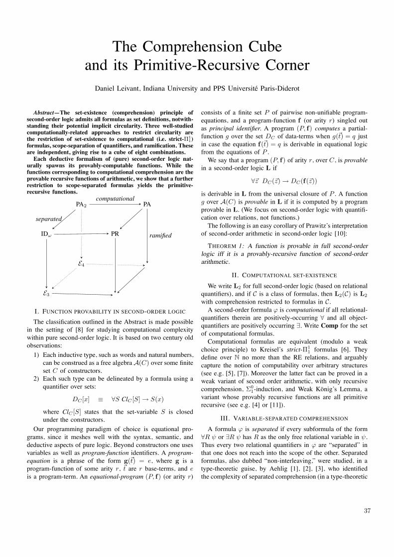
37
The Comprehension Cubeand its Primitive-Recursive CornerDaniel Leivant, Indiana University and PPS Universite Paris-Diderot
Abstract—The set-existence (comprehension) principle ofsecond-order logic admits all formulas as set definitions, notwith-standing their potential implicit circularity. Three well-studiedcomputationally-related approaches to restrict circularity arethe restriction of set-existence to computational (i.e. strict-Π1
1)formulas, scope-separation of quantifiers, and ramification. Theseare independent, giving rise to a cube of eight combinations.Each deductive formalism of (pure) second-order logic nat-
urally spawns its provably-computable functions. While thefunctions corresponding to computational comprehension are theprovable recursive functions of arithmetic, we show that a furtherrestriction to scope-separated formulas yields the primitive-recursive functions.
PA2 PA
IDω PR
E4
E3
computational
separated
ramified
I. FUNCTION PROVABILITY IN SECOND-ORDER LOGICThe classification outlined in the Abstract is made possible
in the setting of [8] for studying computational complexitywithin pure second-order logic. It is based on two century oldobservations:1) Each inductive type, such as words and natural numbers,can be construed as a free algebraA(C) over some finiteset C of constructors.
2) Each such type can be delineated by a formula using aquantifier over sets:
DC [x] ≡ ∀S ClC [S] → S(x)
where ClC [S] states that the set-variable S is closedunder the constructors.
Our programming paradigm of choice is equational pro-grams, since it meshes well with the syntax, semantic, anddeductive aspects of pure logic. Beyond constructors one usesvariables as well as program-function identifiers. A program-equation is a phrase of the form g(!t) = e, where g is aprogram-function of some arity r, !t are r base-terms, and eis a program-term. An equational-program (P, f) (or arity r)
consists of a finite set P of pairwise non-unifiable program-equations, and a program-function f (or arity r) singled outas principal identifier. A program (P, f) computes a partial-function g over the set DC of data-terms when g(!t) = q justin case the equation f(!t) = q is derivable in equational logicfrom the equations of P .We say that a program (P, f) of arity r, over C, is provable
in a second-order logic L if
∀!z DC(!z) → DC(f(!z))
is derivable in L from the universal closure of P . A functiong over A(C) is provable in L if it is computed by a programprovable in L. (We focus on second-order logic with quantifi-cation over relations, not functions.)The following is an easy corollary of Prawitz’s interpretation
of second-order arithmetic in second-order logic [10]:
THEOREM 1: A function is provable in full second-orderlogic iff it is a provably-recursive function of second-orderarithmetic.
II. COMPUTATIONAL SET-EXISTENCEWe write L2 for full second-order logic (based on relational
quantifiers), and if C is a class of formulas, then L2(C) is L2
with comprehension restricted to formulas in C.A second-order formula ϕ is computational if all relational-
quantifiers therein are positively-occurring ∀ and all object-quantifiers are positively occurring ∃. Write Comp for the setof computational formulas.Computational formulas are equivalent (modulo a weak
choice principle) to Kreisel’s strict-Π1
1 formulas [6]. Theydefine over N no more than the RE relations, and arguablycapture the notion of computability over arbitrary structures(see e.g. [5], [7]). Moreover the latter fact can be proved in aweak variant of second order arithmetic, with only recursivecomprehension, Σ0
1-induction, and Weak Konig’s Lemma, avariant whose provably recursive functions are all primitiverecursive (see e.g. [4] or [11]).
III. VARIABLE-SEPARATED COMPREHENSION
A formula ϕ is separated if every subformula of the form∀R ψ or ∃R ψ has R as the only free relational variable in ψ.Thus every two relational quantifiers in ϕ are “separated” inthat one does not reach into the scope of the other. Separatedformulas, also dubbed “non-interleaving,” were studied, in atype-theoretic guise, by Aehlig [1], [2], [3], who identifiedthe complexity of separated comprehension (in a type-theoretic
38
guise) to be that of the theory IDω if finitely-iterated inductivedefinitions [9].This implies quite easily
THEOREM 2: (Essentially Aehlig’s) The functions provablein second-order logic with comprehension restricted to sepa-rated formulas are precisely the provably-recursive functions ofIDω.
Let SepComp be the set of scope-separated computationalformulas.
PROPOSITION 3: Every primitive-recursive function isprovable in L2(SepComp).
Proof Outline. It is an easy exercise to show that if g0 andgs are provable in L2(SepComp), then so is the function fdefined from them by recurrence:
f(0, !y) = g0(!y) f(x + 1, !y) = gs(x, !y, f(x, !y))
The Proposition falls out then by a discourse-level inductionon the generative definition of primitive-recursive functions.!
IV. PROVABLE FUNCTIONS ARE PRIMITIVE RECURSIVEWe prove next the converse of Proposition 3, thereby
establishing our main result:
THEOREM 4: A function is provable in L2(SepComp) iff itis primitive-recursive.
We demonstrate Theorem 4 using standard proof theoretictools, which we assume to be familiar.
LEMMA 5: Fix k ≥ 0. The Normalization Theorem fornatural deductions of L2(SepComp) with ≤ k nested compre-hensions is provable in Primitive Recursive Arithmetic.
Proof Outline. We consider Girard’s proof for the natural-deduction calculus for second-order logic. When deductionsuse only SepComp comprehension, the normalization proofcan itself be formalized in second-order arithmetic with com-prehension restricted to separated computational formulas ofsecond-order arithmetic (where we assume function-identifiersfor all primitive-recursive functions). More precisely, the Nor-malization Theorem for the collection of derivations with ≤ knested instances of SepComp-comprehension can be provedin second-order arithmetic with ≤ k instances of SepComp-comprehension.Consider the theory WKL0 of second-order arithmetic
with Comprehension for recursive formulas, Induction forΣ0
1 formulas, and with Weak Konig’s Lemma (WKL) as anaxiom (stating that every infinite binary tree has an infinitebranch); see e.g. [11], [4]. We can prove within WKL0 thatevery separated computational formula in the the language ofarithmetic is equivalent to a Σ0
1 formula. Thus the Normal-ization Theorem for the collection of derivations with ≤ knested instances of SepComp-comprehension is provable inWKL0. But the Normalization Theorem is a Π0
1 formula
(“every eduction starts some reduction sequence leading toa normal derivation”), and since WKL0 is conservative overPrimitive Recursive Arithmetic with respect to Π0
1 [11], [4],the Lemma follows. !
Proof Outline of the backward implication of Theorem 4.Let (P, f) be a program computing a function g : N → N,and let ∆ be a derivation of N [x] → N [f(x)] from P inL2(SepComp), with ≤ k nested instances of SepComp-comprehension. By Lemma 5 it follows that Primitive Re-cursive Arithmetic proves that for each n ≥ 0 there is anormal derivation Πn of N [n] → N [f(n)] from P . So thereis a primitive recursive function that yields for input n thederivation Πn (suitably coded). Since from Πn we can easilyextract the value of g(n), it follows that g is primitive-recursive. !
V. COMPUTATIONAL COMPREHENSION, UNSEPARTEDWhen comprehension formulas are computational, but not
necessarily variable-separated, we obtain a far larger class offunctions:THEOREM 6: A function if provable in L2(Comp) iff it is
provably recursive in first-order (Peano) Arithmetic, that is iffit is definable by recurrence in all finite types.The backwards implication of Theorem 6 is far more
challenging than Proposition 3, because it is not evident howto interpret first-order arithmetic using comprehension onlyfor computational formulas. We use instead the fact that everyprovably recursive function of PA is definable by transfiniterecurrence over some ordinal α ≺ ε0.The forward direction of Theorem 6 is analogous to that
of Lemma 5, except that the nesting-depth of comprehensioncorresponds to levels in the Arithmetical Hierarchy of theinduction formulas.Acknowledgment. This work was also supported by LORIANancy.
REFERENCES[1] Klaus Aehlig. On fragments of Analysis with strengths of finitely iterated
inductive definitions. PhD thesis, Ludwig-Maximilans-Universit”at,2003.
[2] Klaus Aehlig. Induction and inductive definitions in fragments of secondorder arithmetic. J. Symb. Log., 70(4):1087–1107, 2005.
[3] Klaus Aehlig and Jan Johannsen. An elementary fragment of second-order lambda calculus. ACM Transactions on Computational Logic,6:468–480, 2005.
[4] Jeremy Avigad and Solomon Feferman. Godel’s functional (dialectica)interpretation. In Samuel Buss, editor, Handbook of Proof Theory, pages337–405. North-Holland, Amsterdam, 1988.
[5] Jon Barwise. Admissible sets and structures. Springer-Verlag, Berlin,1975.
[6] G. Kreisel. Mathematical logic. In T. Saaty, editor, Lectures on ModernMathematics, volume III, pages 95–195. John Wiley, New York, 1965.
[7] Daniel Leivant. Descriptive characterizations of computational complex-ity. J. Comput. Syst. Sci., 39(1):51–83, 1989.
[8] Daniel Leivant. A foundational delineation of poly-time. Informationand Computation, 110:391–420, 1994.
[9] Wolfram Pohlers. Subsystems of set theory and second order numbertheory. In Samuel Buss, editor, Handbook of Proof Theory, pages 209–335. North-Holland, Amsterdam, 1988.
[10] D. Prawitz. Natural Deduction. Almqvist and Wiksell, Uppsala, 1965.[11] Stephen Simpson. Subsystems of Second Order Arithmetic. Springer-
Verlag, Berlin, 1999.
39
On the Expressivity of Linear Logic SubsystemsCharacterizing Polynomial Time
Matthieu PerrinelLaboratoire d’Informatique du Parallelisme
ENS Lyon – Universite de Lyon UMR 5668 CNRS ENS-Lyon UCBL INRIA46, allee d’Italie 69364 Lyon cedex 07 – FRANCE
Abstract—Implicit computational complexity characterizes
complexity classes by restricting models of computation (lambda
calculus, recursion theory, linear logic,...).
All previously studied subsystems of linear logic characterizing
Ptime lack expressive power. Although every Ptime function can
be computed in those systems, they do not always accept the most
usual algorithms. In this work we will approach the “expressivity
frontier”: the sets of programs that could be accepted by Ptime
sound linear logic subsystem.
I. INTRODUCTION
a) Implicit computational complexity: For decades, com-puter scientists have tried to characterize classes of complexityby restricting syntactically models of computation. This effortis known as implicit computational complexity. The main goalis to achieve automated certification of the complexity of aprogram. Some consider also other goals for implicit compu-tational complexity: to understand the roots of complexity, assuggested by Dal Lago [7] or to create polytime mathematics,as suggested by Girard [3].
Many characterizations of polynomial time have been foundfor different models of computation: restriction of recursion [2], non-size-increasing computation [5], quasi-interpretations ona functional language and restriction of linear logic [6] [3] [1].Each approach has its own assets and drawbacks with respectto our goal of statically inferring bounds on real-life programs.
b) Linear logic and expressivity: One of the interests ofthe linear logic approach is the possibility to quantify overtypes (second order types). This allows us, for example, towrite a sorting algorithm which can be applied to any typeof data, as soon as a comparison function is given. The firstreally implicit characterization of polynomial time by a linearlogic subsystem was Light Linear Logic (LLL) by Girard [3].
The main drawback of LLL is the lack of expressivity.A completeness result shows that any Turing machine ter-minating in polytime can be simulated by a LLL proof-net (proof-nets are the programs of linear logic). Howeverwe cannot expect programmers to stick to the simulation ofTuring machines. Therefore, we are more interested in theprogramming of high-level algorithms, but many of thoseare not typable in LLL. And many of those algorithms arenot typable in LLL (for example the usual multiplication onChurch integers and quick-sort). Among the other linear logiccharacterizations of Ptime, SLL [6] is even less expressive
than LLL. L4 and L40 [1] generalize LLL, but the increase in
expressivity is very limited.Therefore, we can wonder if the lack of expressivity is a
drawback of the current subsystems (SLL, BLL, LLL, L4,L40) or a limitation inherent to the linear logic approach? If
there are usual algorithms which are not accepted by anyPtime linear logic subsystem, then it would raise doubts on theusability of the linear logic approach for real life applications.In this work, we give a sufficient criterium for Ptime which wethink is broader than previous criteria. We also give a sufficientcriterium for elementary time (towers of exponentials of fixedheight), and a necessary criterium for elementary time, relatedto the sufficient criterium. Those criteria are based on DalLago’s context semantics [7].
c) Context semantics: The idea of geometry of interac-tion [4] and context semantics is to study the reduction ofproof-nets (or �-terms) by leaving the proof-net unchangedand analysing instead some paths in it. Context semantics hasfirst been used to study qualitative properties. In [7], Ugo DalLago adapted context semantics to study quantitative proper-ties of cut-reduction. From this point of view an advantage ofcontext semantics compared to the syntactic study of reductionis its genericity: some common results can be proven fordifferent variants of linear logic, which allows to factor outproofs of complexity results for these various systems. Indeedstrong bounds were proven in context semantics for SLL,ELL, LLL, and L4.
A side effect of this proof factorization is the emergence ofa common structure in those proofs, and gives a new point ofview on them. Context semantics gives semantics character-ization of the “stratification” condition and the “dependencecontrol” condition pointed out by Baillot and Mazza [1].
II. CHARACTERIZATION OF STRATIFICATION ANDDEPENDENCE CONTROL
d) Context semantics characterization of stratification:
The idea of stratification is to forbid self-duplication. Wedefine a duplication relation on boxes and we define stratifiedproof nets as the proof nets whose duplication relation isacyclic.
In the following definition, �(B) refers to the edge leavingthe principal door of box B. �i(B) refers to the edge leavingthe i-th auxiliary door of box B.
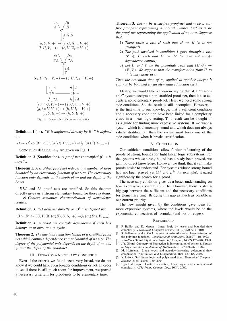
40
`Aa
Bb
A`Bc
(a, U, V,+) 7! (c, U,`l :: V,+)(b, U, V,+) 7! (c, U,`r :: V,+)
?C?A
e1?A
e2
?Ag
(ei, U, ?t :: V,+) 7! (g, U, ?i.t :: V,+)
?P
Ae
?Af
!P
Ag
?Ah(e, t � U, V,+) 7! (f, U, ?t :: V,+)(g, t � U, V,+) 7! (h, U, !t :: V,+)
(f, U, !t,�) 7! (h, U, !t,+)
Fig. 1. Some rules of context semantics
Definition 1 (⇣). ”B is duplicated directly by B0” is defined
by:
B ⇣ B0 , 9U, V, 9t, (�(B), U, !t,+) 7!⇤G (�(B0), V, ,�).
Some rules defining 7!G are given on Fig. 1.
Definition 2 (Stratification). A proof net is stratified if ⇣ is
acyclic.
Theorem 1. A stratified proof net reduces in a number of steps
bounded by an elementary function of its size. The elementary
function only depends on the depth of ⇣ and the depth of the
boxes.
ELL and L3 proof nets are stratified. So this theoremdirectly gives us a strong elementary bound for those systems.
e) Context semantics characterization of dependence
control:
Definition 3. ”B depends directly on B0” is defined by:
B < B0 , 9U, V, 9t, (�(B), U, !ti ,+) 7!⇤G (�i(B
0), V, , )
Definition 4. A proof net controls dependence if each box
belongs to at most one < cycle.
Theorem 2. The maximal reduction length of a stratified proof
net which controls dependence is a polynomial of its size. The
degree of the polynomial only depends on the depth of ⇣ and
< and the depth of the proof-net.
III. TOWARDS A NECESSARY CONDITION
Even if the criteria we found seem very broad, we do notknow if we could have even broader conditions or not. In orderto see if there is still much room for improvement, we proveda necessary criterium for proof-nets to be elementary time.
Theorem 3. Let ⇡0 be a cut-free proof-net and n be a cut-
free proof-net representing a natural number. And let ⇡ be
the proof-net representing the application of ⇡0 to n. Suppose
that:
1) There exists a box B such that B ⇣ B (⇡ is not
stratified).
2) The path involved in condition 1 goes through a box
B0 2 B such that B0 � B0(⇡ does not satisfy
dependence control).
3) Let U and V be the potentials such that (B,U) ⇣(B, V ). We suppose that the transformation from U to
V is only done in n.
Then the execution time of ⇡0 applied to another integer kcan not be bounded by an elementary function on k.
Ideally, we would like a theorem saying that if a “reason-able” system accepts a non-stratified proof-net, then it also ac-cepts a non-elementary proof-net. Here, we need some strongside conditions. So, the result is still incomplete. However, itis the first time to our knowledge, that a sufficient conditionand a necessary condition have been linked for a complexityclass, in a linear logic setting. This result can be thought ofas a guide for finding more expressive systems. If we want asystem which is elementary sound and which does not alwayssatisfy stratification, then the system must break one of theside conditions when it breaks stratification.
IV. CONCLUSION
Our sufficient conditions allow further refactoring of theproofs of strong bounds for light linear logic subsystems. Forthe systems whose strong bound has already been proved, wegain no direct knowledge. However, we think that it can makeproofs easier to understand. For systems whose strong boundhad not been proved yet (L4 and L3a for example), it easedsignificantly the search for a proof.
The necessary condition gives us a better understanding onhow expressive a system could be. However, there is still abig gap between the sufficient and the necessary conditionsfor elementary time. Bridging this gap as much as possible isour current priority.
The new insight given by the conditions gave ideas formore expressive systems, where the levels would be on theexponential connectives of formulas (and not on edges).
REFERENCES
[1] P. Baillot and D. Mazza. Linear logic by levels and bounded timecomplexity. Theoretical Computer Science, 411(2):470–503, 2010.
[2] S. Bellantoni and S. Cook. A new recursion-theoretic characterization ofthe polytime functions. Computational complexity, 2(2):97–110, 1992.
[3] Jean-Yves Girard. Light linear logic. Inf. Comput., 143(2):175–204, 1998.[4] J.Y. Girard. Geometry of interaction 1: Interpretation of system f. Studies
in Logic and the Foundations of Mathematics, 127:221–260, 1989.[5] M. Hofmann. Linear types and non-size-increasing polynomial time
computation. Information and Computation, 183(1):57–85, 2003.[6] Y. Lafont. Soft linear logic and polynomial time. Theoretical Computer
Science, 318(1-2):163–180, 2004.[7] Ugo Dal Lago. Context semantics, linear logic, and computational
complexity. ACM Trans. Comput. Log., 10(4), 2009.

