library - defense technical information center · laboratory at annapolis, ... 3.11 plate bending...
TRANSCRIPT

GVTDOCD 211.9:4057
NAVAL SHIP RESEARCH AND DEVELOPMENT CENTER TBethesda, Md. 20034
STRESS ANALYSIS OF COMPLEX SHIP COMPONENTS
BY A NUMERICAL PROCEDURE USING
CURVED FINITE ELEMENTS
by
James Hsienne Ma OCT
U. S. NAP/VM CCADEMY
APPROVED FOR PUBLIC RELEASE: DISTRIBUTION UNLIMITED
STRUCTURES DEPARTMENT
RESEARCH AND DEVELOPMENT REPORT
LIBRARY
July 1973 DEC 5 1973 Report 4057
-0

The Naval Ship Research and Development Center is a U. S. Navy center for laboratoryeffort directed at achieving improved sea and air vehicles. It was formed in March 1967 bymerging the David Taylor Model Basin at Carderock, Maryland with the Marine EngineeringLaboratory at Annapolis, Maryland.
Naval Ship Research and Development Center
Bethesda, Md. 20034
MAJOR NSRDC ORGANIZATIONAL COMPONENTS
NSRDC
COMMANDER 00
"*REPORT ORIGINATOR TECHNICAL DIRECTOR
01
OFFICER-IN-CHARGE OFFICER-IN-CHARGECARDEROCK 05 ANNAPOLIS 04
SYSTEMSDEVELOPMENTDEPARTMENT
SHIP PERFORMANCE AVIATION ANDDEPARTMENT SURFACE EFFECTS
15 DEPARTMENT
16
SSTRUCTURES COMPUTATION
DEPARMENTAND MATHEMATICS
DEARMET 17 DEPARTMENT 18
SHIP ACOUSTICS PROPULSION AND
DEPARTMENT AUXILIARY SYSTEMS19 DEPARTMENT 27
MATERIALS CENTRAL
DEPARTMENT INSTRUMENTATION28 DEPARTMENT
29
NDW-NSRDC 3960/43b (Rev. 3-72)
GPO 928-108

DEPARTMENT OF THE NAVY
NAVAL SHIP RESEARCH AND DEVELOPMENT CENTERBETHESDA, MD. 20034
STRESS ANALYSIS OF COMPLEX SHIP COMPONENTS
BY A NUMERICAL PROCEDURE USING
CURVED FINITE ELEMENTS
by
James Hsienne Ma
APPROVED FOR PUBLIC RELEASE: DISTRIBUTION UNLIMITED
July 1973 Report 4057

TABLE OF CONTENTS
Page
ABSTRACT . . . . . . . . . . . . . . . . . . . . . . . . . . . . . . I
ADMINISTRATIVE INFORMATION ................. ...................... I
CHAPTER
I INTRODUCTION ...................... ........................ 31.1 General ........................ .......................... 31.2 Objective and Scope ................... ...................... 41.3 N otations . . . . . . . . . . . . . . . . . . . . . . . . . 5
2 THE FINITE ELEMENT METHOD OFSTRUCTURAL ANALYSIS ............. .................... 11
2.1 Background ................. ......................... .. 112.2 Finite Element Displacement Approach ........ ............... .. 12
2.2.1 Element Analysis ............. ..................... .. 122.2.2 Structural Analysis (by Direct Stiffness Method) .... .......... .. 14
2.3 Characteristics of Finite Element Analysis ...... .............. .. 152.3.1 Convergence Criteria .......... ................... .. 152.3.2 Elements of Arbitrary Shapes ........ ................ .. 16
3 ELASTIC ANALYSIS IN THREE-DIMENSIONAL SPACE .... .......... 193.1 Introduction to Solid Elements .......... .................. .. 193.2 The Basic Solid Elements ............ .................... .. 19
3.2.1 The Isoparametric Displacement Field ....... ............. .. 213.2.2 Numerical Calculation of Stiffness Matrix ...... ............ 253.2.3 Higher Order Curved Elements .......... ................ 30
3.2.3.1 Quadratic Curved Element ....... .............. .. 303.2.3.2 Cubic Curved Element ......... ................ .. 32
3.2.4 Practical Considerations ............ .................. 323.3 Specialization ................ ......................... 33
3.3.1 Load Matrix for a Prescribed Pressure ..... .............. ... 333.3.2 Stresses on an Arbitrary Surface ........ ............... .. 383.3.3 Applications to Plates and Shells ........ ............... .. 42
3.4 Implementation .............. ....................... .. 423.4.1 Introduction to Solution Methods ....... ............... .. 473.4.2 Frontal Technique ............ .................... .. 48
3.5 Evaluation of Numerical Results ........... .................. .. 513.5.1 Prismatic Beams ............. ..................... .. 52
3.5.1.1 A Cantilever Beam .......... ................. .. 523.5.1.2 A Simply Supported Beam ...... .............. .. 52
3.5.2 Plate Bending ............... ...................... .. 553.5.3 Thick-Walled Cylinder ........... ................... .. 583.5.4 Stiffened Plates .............. ..................... .. 58
4 SPECIAL CLASS OF STRUCTURAL PROBLEMS ...... ............. .. 674.1 Introduction to Propeller Blades ........... .................. .. 674.2 The Geometry of Skewed Propellers ........ ................ .. 684.3 Experimental Data ................ ...................... 734.4 Finite Element Analyses .............. .................... 754.5 Discussion of Results ............. ..................... .. 82
CONCLUSIONS AND RECOMMENDATIONS ......... .............. 87
ii

Page
ACKNOWLEDGMENT ................... .......................... 89
REFERENCES ...................... ............................. .. 95
APPENDIX - EXAMPLE OF FORTRAN PROGRAM FOR NUMERICALCALCULATION OF AN ELEMENT STIFFNESS MATRIX ... ......... .. 91
LIST OF FIGURES
Figure
3.1 Tetrahedron, a solid element and rectangular coordinate system ... .......... ... 20
3.2 An eight-node generalized hexahedron .......... .................. .. 22
3.3 Refined curved hexahedron .............. ...................... .. 23
3.4 Curved element representation of a complex surface ..... .............. ... 34
3.5 Rotation of reference frame ............. ...................... .. 39
3.6 Element nodal incidence and local reference frame ........ .............. .. 39
3.7 A quadric curved shell element ............. ..................... .. 43
3.8 Stiffness matrix of a structural system (solution by theGauss frontal technique) ................ ....................... .. 49
3.9 Frontal processing of a finite element idealization of thecross frame of a ship ...................... ........................ 50
3.10 Pure bending of a prismatic bar ............. ..................... .. 53
3.11 Plate bending sample problem (example 3.1) ........ ................ .. 56
3.12 Convergence of center deflection of a square plate with meshrefinement (example 3.1) ............... ....................... .. 57
3.13 Distribution of bending moments along a center line of asquare plate (example 3.1) .............. ...................... 57
3.14 Stiffened plate sample problem (example 3.2) ......... ................ .. 61
3.15 Distribution of normal stresses in a plate beam (example 3.2) .... .......... 62
4.1 Global coordinate system used in definition of skewed propeller ... ......... .. 69
4.2 XY-plane projection of a propeller blade (looking forward) .... ........... .. 69
4.3 Local blade coordinate systems (x, y, Z) and (p, 0, Z) ..... ............. .. 71
4.4 Developed view of cylindrical blade section .... ......... ........... .. 72
4.5 Aluminum blade model (looking forward) .......... ................. .. 74
4.6 Interferometric fringe pattern of blade model with applied pressure ( 0.098 psi) . . .. 74
iii

Page
Figure
4.7 Projected view of two 5-bladed model propellers (model propellerseries, part I) ................... ........................... .. 76
4.8 XY- and YZ-projections of a highly skewed propeller blade .... ........... .. 77
4.9 Curved solid element representation of a 72-degree skewedpropeller blade .................. .......................... 78
4.10 Computed and measured displacements of a 72-degreeskewed propeller ................. .......................... .. 80
4.11 Stresses of a 72-degree skewed propeller ........... .................. .. 83
4.12 Flat shell element representation of a 72-degree skewedpropeller blade .................. .......................... 84
LIST OF TABLES
Table
3.1 Results of analysis of a simply supported beam ....... ............... .. 54
3.2 Results of stress calculations for a thick-walled cylinder ..... ............ .. 59
3.3 Longitudinal stresses in a stiffened plate(example 3.2) ................... ........................... .. 63
iv

ABSTRACT
A numerical procedure for the structural analysis of a general three-
dimensional nature has been developed to provide a reliable solution to the
problem of determining the strength of propellers, particularly those with
unconventional configurations. A finite element displacement model is utilized
and compatible solid elements in their general form are adopted. The use of
interpolation functions to define pertinent curvilinear coordinates in element
space gives the finite element technique, new capabilities for dealing with
structures of highly complex geometry. This formulation bypasses the con-
straints of simplifying assumptions (such as those imposed by classicial plate
theory) and allows a closer approximation to the true structural configuration
than is possible by other approaches, including most analytical and numerical
methods. The performance of the refined elements described in this report is
distinctly superior to those obtainable with commonly available elements, for
example, those in NASTRAN. A highly skewed propeller blade under pre-
scribed pressure distributions was chosen for demonstration of the generality
of the procedure. Good agreement was obtained with measured displacement
and experimental stress data.
ADMINISTRATION INFORMATION
The studies described in this report were carried out from the fall of 1971 to the fall of 1972 at
the Naval Ship Research and Development Center (NSRDC) and were sponsored by the Naval Ship
Systems Command (NAVSHIPS). Funding was provided under Subproject SF 43 422 312, Task 15084
(Structural Analysis for High Performance Surface Ships), Work Unit 1-1730-089.
The material contained in this report was submitted to the Graduate College of the University of
Illinois at Urbana-Champaign in partial fulfillment of requirements for the degree of Doctor of Philosophy
in Civil Engineering. The headings and other details of format follow University of Illinois rather than
NSRDC style.

CHAPTER 1
INTRODUCTION
1.1 General
Recent years have witnessed an increased interest in the development of performance-
oriented surface ships for which it is vital to keep weight to a minimum, e.g., high-speed
hydrofoils, catamarans, and surface effect ships. A more accurate method of analysis than
currently employed in shipyards is imperative if weight saving is to be achieved for such
vehicles. The effective use of materials and an increased reliability of design will have
far-reaching results over their life spans.
Governed by functional requirements and hydrodynamical considerations, the geometry
of ship scantlings is generally complex and their construction contains a high degree of
redundancy. It is therefore necessary to make simplifying assumptions in order to reduce
the complexity of the mathematical model representing the structure to a form that is amenable
to traditional design methods. In consequence, certain characteristic behavior of the elastic
body is ignored and the accuracy of the analysis is often open to question. Thus verification
requires testing scaled models and, at times, costly prototypes as well.
The rapid advances in digital electronic computers since the mid-1950's coupled with
recent development in discrete element methods provide a powerful new tool for structural
analysis (Paulling, 1964; Moe and Tonnesen, 1966; and the International Ship Structures
Committee, 1969).* Many complicated design problems that were considered insurmountable
to a realistic analysis only a few years ago can now be executed almost routinely by using
an ordinary computer (Roren, 1969; Ma, 1969; and Abrahamsen, 1970). Specifically a struc-
ture system having, say, 1000 degrees of freedom can be solved in a matter of a few min-
utes on a late model computer (such as CDC 6600, or IBM 360/75, etc.) through appropriate
idealization with due consideration for the bandwidth of the resulting system of equations.
During the past decade, the development of finite element methods has exhibited an
exponential growth, and the demand for appropriate programs has increased rapidly. The
total number of finite element computer programs in which substantial efforts have been ex-
pended may have exceeded several hundred (Gallagher, 1970 and Schrem, 1971). Neverthe-
less, only a rather small number of them (and these only recently) are accessible to engi-
neers in practice. Among these well known programs are NASTRAN, the NASA structural
analysis (MacNeal and McCormick, 1967); STRUDL, structural design language (Logcher
and Sturman, 1966); FINEL (Adamchak, 1970) and SAMIS (Melosh et al., 1966). Programs of
a proprietary nature includes ASKA (Schrem and Roy, 1971); DAISY (Kamel et al., 1969);
SFSAM-69 (Araldsen and Egeland, 1971); SAP (Wilson, 1970); STARDYNE (Dainora, 1971);
and others (Hartung, 1970; and Mallett and Jordan, 1969).
*References are listed alphabetically starting on page 95.
3

Mo st of the finite element programs, including larger scale and general purpose pro-
grams that; are currently available, have little or no data-generation features and their ele-
ment libraries contain basically one- and two-dimensional elements of linear or constant-
strain type~s. The big cost item of a finite element analysis is frequently the data preparation
stage. In areas of steep stress gradient, for example, the good approximation of an important
structural response may require the assemblage of a large number of elements, especially
when the elenernts to be used are of lower calibre, such as the constant-stress elements. In
the case of an ii~regular boundary, curved elements will have a distinct advantage. Thus re-
finement of element characteristics can have a profound impact on the economy and range of
solution that the finite element method can provide.
By nature of their geometric proportions, many structural components can be idealized
as one- or two-dim ensional problems of elasticity and standard methods can be used to obtain
reasonably good solutions. For other design tasks, however, no conventional approach can
achieve realistic rcsults. Examples are bodies of complex, unsymmetrical shapes and inter-
face problems of two or more geometrical entitles (e.g., the junction of pipes, plates, and/or
shells). The rational solution of such problems requires a general analysis in three-
dimensional elast icity. It is in this difficult, but important, field of three-dimensional prob-
lems that recent developments in the isoparametric element family offer the most promising
approach. These refined elements will be utilized in the study reported here.
1.2 Objective and Scope
The objective of the present, study was to develop a numerical procedure for the static
analysis of a three- dimensional elastic body of arbitrary configuration. More specifically,
the purpose was to (determine the structural behavior of a marine propeller subjected to a pre-
scribed pressure loa(ding. A highly skewed propeller* was chosen to dcmron:Jst•'te the gever,
ality of the approach. The study employed the finite element method in conjunction with
curved solid elements,, A computer program was developed to implement the procedurc for
predicting displacemerits and stresses of a complex structure itb refeoence to an arbitrary
curvilinear coordinate Bystem. Linear elas•ticity and small deformation theory were ussumed.
Chapter 2 outlinos the finite el(hent method for structural analysis. Certain element
characteristics derived f,"om a displacement model are discussed to aid in the selection of
appropriate elements for improved computational results.
Although finite el ement techniques are widely used in the two-dimensional domain of
plates and shells, they have had only limited application for the treatment of complex struc-
tures in the context of three-dimensional elasticity. The principal reason for this slow
*The marine propeller takes on complex, skewed geometry as a result of design considerations, such as thoseof vibration and cavitation aspet s in blade design (Cox and Morgan, 1972).
4

progress is the large amount of input data and processing time required to implement a three-
dimensional solution when only simple, tetrahedron-type solid elements are utilized. Isopara-
metric formulation and its associated refined curved elements coupled with a more efficient
solution technique (as described in Chapter 3) now make it possible to tackle some of the
most difficult problems in solid mechanics.
Some selected problems, including beams, plates, shells, and stiffened plates are
solved to evaluate the adequacy and performance of the procedure developed here. Further,
a ship component of complex geometry-a skewed propeller blade-is analyzed in Chapter 4
to provide insight into the potential of the procedure as a design tool. Since no analytic
solution for the propeller blade problem is known, computed results for displacements and
stresses are compared with experimental data.
1.3 Notations
The symbols used in this study are defined where they first appear. For convenience,
frequently used symbols are summarized below.
The bar and tilde underscores (or overscores) generally denote a vector and a matrix,
respectively. Parentheses and brackets are used alternatively to denote a vector and a
matrix. For example, a column vector Ua can be written
U 1
with its subvector
-Pi =lUll = V•
A matrix
A A A
0 = [0] = [V1 , V2 , V 31
When vector quantities appear in an equation, standard vector notations will apply. For
example, "x" and "." represent cross and scalar product of vectors, respectively.
5

[A] matrix of functions in nodal coordinates, Eq. (2.2)
[B] matrix relating strain vector to nodal displace-ments, Eq. (2.4) or (3.8)
[B'] matrix relating local strain vector of a shell tonodal displacements, Eq. (3.52)
D a specified domain, such as a given volume or area
[D] elasticity matrix
[D ] elasticity matrix in the local coordinate system fora isotropic shell element
EDK
(1 + v) (1 - 2 v)
E Young's modulus of elasticity
{FI equivalent load vector, also known as generalizedload vector
FX, FY, FZ equivalent element nodal force in the x, y, or adirection, respectively; forces are positive inthe positive direction of x, y, and z axes
Fx (1), F y (I), Fz (1) equivalent force in direction of x, y or 2 axis atnode "i," Eq. (3.28)
[g (el, 7, 1)] matrix containing functions of curvilinear coordinates
EC = shear modulus of elasticity2(1 + v
Hix, Iy, Hiz weighting coefficient corresponding to position alongGaussian quadrature points ýi ,i y or Ciz
i subscript indicating nodal number, or active index
I moment of inertia of a transverse section of a beam
A A A
i, ], k vector having unit value in direction of x, y, orz axis, respectively
[J] Jacobian matrix of coordinate transformation
I.l Jacobian determinant
6

k constant factor included in [D '] matrix to improveshear deformation
kl., stiffness coefficient at i th row and j th column
[K] stiffness matrix of entire structure
[Ke] stiffness matrix of an element e
K (r. s) submatrices of [K]
A AA
Pm, n direction cosines of a unit vector e and (i, J, k)representing global rectangular axes (x, y, z)
[La] localizing matrix relating element nodal parameterto global structure parameter, Eq. (2.13)
MX, M7 Ybending moment components in the x and y directions
n vector normal to a curved surface
N 77), Ni(4, 7 7) function of curvilinear coordinates in two or threedimensions, respectively, taking a value of unityat node i and zero at all other nodes
NNPE number of nodes per element
T applied pressure on an element face, Eq. (3.27)
{PI global load vector (entire structure)
[Pa external load vector for an element
P•, P7, PC vectors tangent to curvilinear coordinate lines(67, 4)
q (x, y, z) intensity of distributed loads
[q] column matrix of generalized coordinates
A A A
7 displacement vector (= ui + vj + wk)
displacement vector of node "i"
[R] rotation matrix for coordinate transformation,Eq. (3.40)
S area of curved surface
7
t. shell thickness at node i
u, v, w components of displacement in the direction of x, y and aaxes, respectively; displacements are positive in thepositive direction of coordinate axes
ui, vi, wi components of displacement at node i
IN} vector of nodal parameters for entire structure, Eq. (2.13)
jUal nodal displacement vector for an element
U. vector of parameters at node i
U1. S vector of parameters at node i for shell element,Eq. (3.51)
A A A
V1, V2 , V3 unit vectors in directions of local axes x , and 2',
respectively
A A A
Vli, V 2 0, V3 i local unit vectors at node i
V3 i shell thickness vector at node i
Vol volume of a given solid domain
we work done by external load
w 1.internal work of strain energy
x1, y, ? global system of rectangular coordinates
x , y , 2' local system of rectangular coordinates for shell element
Xi. Yil zi coordinates at node i
a, 1P rotations of nodal normal about two orthogonal axes
ail Pii rotations of normal at node i
la}I column matrix of constant coefficients, Eq. (3.21)
Yxy, YYZ, Yxz shearing strain components
Yx.*'yl 1',Y'z, Yxpz shearing strain components in the local rectangularcoordinates
8
a prefex denoting first variation of a function
SU. virtual displacement at node i for an element
[I ] local strain tensor, Eq. (3.42)
local strain vector for a shell element Eq. (3.52)
4 a curvilinear coordinate in the thickness direction in caseof a shell element
4, i1, curvilinear coordinates at any point within an element
41., tii ei curvilinear coordinates at node i
Ciz' niyl ýix position constants for the Gaussian quadrature point i
[0] direction casine matrix of a local orthogonal system ofaxes
v Poisson's ratio
[a] stress tensor, Eq. (3.43)
rxPy,, rypzP, rzP P shearing stress components in the local rectangularcoordinates
[1 (X, y, z)] row matrix of monomial functions of cartesian coordinate,Eq. (3.1)
summation on the running index i
f
fD integration over a domain D
9

CHAPTER 2
THE FINITE ELEMENT METHOD OF STRUCTURAL ANALYSIS
2.1 Background
The finite element methods of structural mechanics rely heavily on numerical compu-
tation and their advent followed the availability of high-speed digital computers. The matrix
formulation of structural problems was formally introduced by J. H. Argyris in a series of
papers published in 1954-55. About the same period, notable progress in applying finite ele-
ment methods to the analysis of aircraft and civil engineering structures had been made inde-
pendently by a number of investigators including M. J. Turner (1956) and his group at the
Boeing Company and B. Langefors (1958) in Sweden.
The basic concept of the finite element method is that a real continuum can be treated
analytically by subdividing it into a finite number of regions. In each of these regions, the
behavior, such as displacement or stress, is described by a separate field. These fields are
often chosen in a form that ensures continuity of the described behavior throughout the com-
plete continuum. In other cases, the chosen fields do not ensure continuity but nevertheless
they achieve satisfactory solutions. These later cases do not have the assurance of converg-
ence* possessed by the fully continuous analytical models (Melosh, 1963 and Irons and Draper,
1965). The concept of the finite element representation owes much to the early work ofA. P. Hrenikoff (1941) and R. Courant (1943); the later was concerned with problems governed
by broader field equations than just structural mechanics.
Much progress had been made in the various aspects of finite element analysis. Im-
proved results were realized by introducing new types of elements, such as more powerful
refined elements (Argyris, 1965; Felippa, 1966; Mehrain, 1967; Kohnke and Schnobrich,
1969; and Chu and Schnobrick, 1970) or efficient superelements (Araldsen and Egeland,
1971). Successful developments were also cited for various forms of structural behavior
representation as in dynamics, plasticity, and large deflection (Argyris, 1965; Przemieniecki
et al., 1971; and Zienkiewicz, 1971).
The formulation of the finite element method can be traced to energy procedures, prin-
cipally the minimum potential energy (MPF) method and the minimum complementary energy
(MCE) method. The MPE method is associated with assumed displacement parameters as un-
knowns and is usually termed the "displacement" or "stiffness" method. On the other hand,
the MCE method deals with stress parameters and is termed the "flexibility" approach. Sev-
eral authors, e.g., Fraeijs deVeubeke (1964), have been concerned with a parallel use of dis-placement and equilibrium models to obtain lower and upper bounds to the exact solution.
Still others (Fraeijs deVeubeke, 1964 and Herman, 1967) used a mixed model and considered
both displacements and stresses as primary variables. The ease with which a continuous
*For convergence requirements, see Section 2.3.1.
11

displacement pattern can be prescribed (compared to the alternative approach of forming an
equilibrating internal force field) has aided the widespread use and development of the finite
element displacement approach. The displacement model and the stiffness analysis are em-
ployed in the present study.
2.2 Finite Element Displacement Approach
The displacement formulation involves derivation of the stiffness matrix of each indi-
vidual element. The stiffness matrix of the entire assembled structure is then obtained by
the direct stiffness method. This matrix, along with the prescribed displacement boundary
conditions and loads, is used for the solution of displacements and stresses.
2.2.1 Element Analysis
The basic steps for derivation of the element stiffness matrix are:
a. Express the internal displacements WUI of the element in terms of displacement func-
tions q5(x, y, 2), and generalized coordinates IqI
[UI = [ ] q1 (2.1)
where U (X, y, 2)
IUI V (X, Y, P')
W(X, y, 2)
is a displacement vector consisting of displacement components u, v, w, referenced to the
rectangular cartesian coordinate system (x, y, 2).
b. Express the nodal displacements IUa} in terms of generalized coordinates Iql:
j~aj = [A] IqI (2.2)
Here {Ua} = {Ui(x, y, z)l and
Ui(X, y, 2) = U (xi, Yj, zi) i = 1, ,.. , n
are the displacements at node "i" and n is the number of nodes. Coefficients of matrix [A]
are functions of nodal coordinates (xi, Yi, ;?)" Conversely,
IqI = [A]-' Ial (2.3)
12
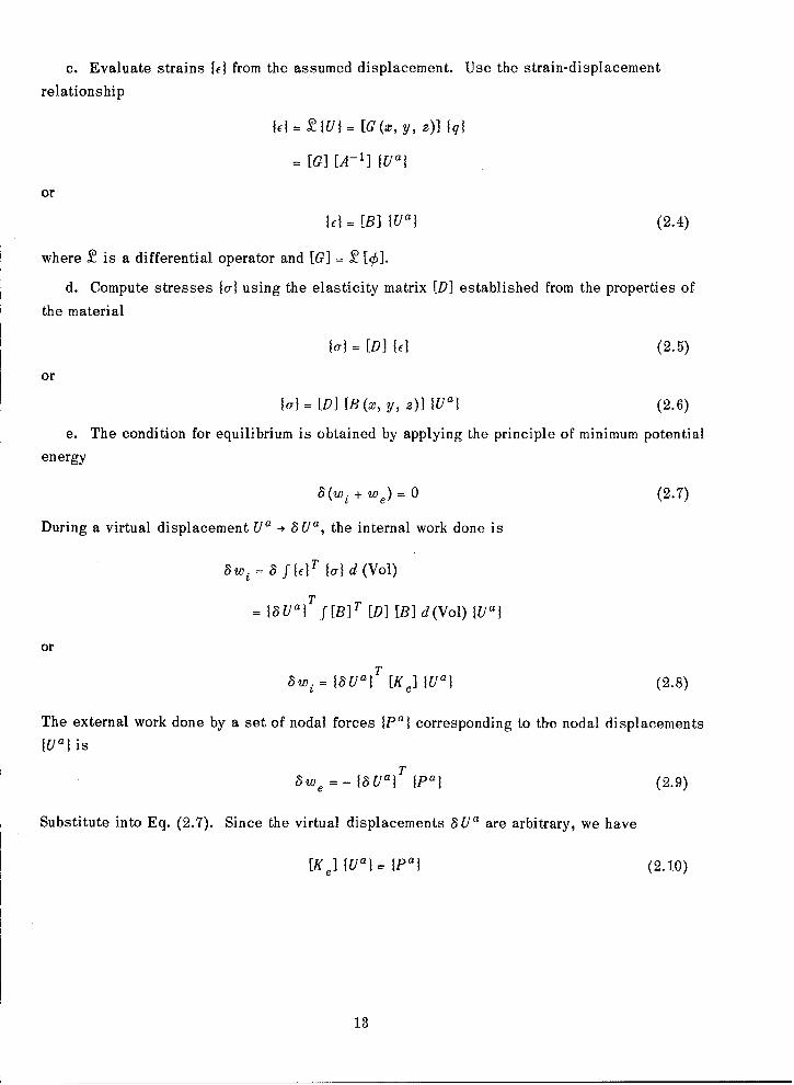
c. Evaluate strains {li from the assumed displacement. Use the strain-displacement
relationship
Jcj- = 2el-- [G(x, y, z)] Ill
= [G] [A-'] IUal
or
= [B] jUal (2.4)
where 2 is a differential operator and [G] = 2 [o].
d. Compute stresses Jul using the elasticity matrix (D] established from the properties of
the material
lal = [D] Id (2.5)
or
Jul = [D] [B(x, y, z)] tUal (2.6)
e. The condition for equilibrium is obtained by applying the principle of minimum potential
energy
6(wi + We) = 0 (2.7)
During a virtual displacement U' -* aUa, the internal work done is
awi = fEIT Jal d (Vol)
= lauaT f[B]T [DI [B] d(Vol) {Ual
or
awi = IbUali [Ke] IUal (2.8)
The external work done by a set of nodal forces IPaI corresponding to thre nodal displacements
jUal is
Tawe -8Ua Plal (2.9)
Substitute into Eq. (2.7). Since the virtual displacements 8Ua are arbitrary, we have
[Ke] IUaI = lPa (2.10)
13

where [KWe = f [B]T [DI [B] d(Vol)T
= [A1] f [G] T [D] [G] d(Vol) [A-'] (2.11)
expresses the nodal force-displacement relation and is the desired element stiffness matrix.
f. Establish the load generalization. Generally loads are distributed. Concentrated
loads at nodes represent special cases. In the finite element context where all the forces
can be transmitted only through the prescribed network of nodes, we need to compute the
equivalent concentrated nodal loads 1paI for the actual distributed loading p (x, y, a).
Equivalence is based on the work done during a virtual displacement consistent with the
assumed displacement field U (x, y, ?). Since
6we = - 3f U17 JpJ d (Vol)
Eq. (2.9) gives the equivalent loading vector
1p I = [A-,] fk[]T Ip d(Vol)
or
P' I = f[N]rTpI d(Vol) (2.12)
The vector {Pfl is often called the generalized load of element "a" and N is known as shapefunction. Thus a normal load can produce not only parallel nodal forces but also couples, or
their equivalent, and these will depend on the displacement assumption U (x, y, a) used.
2.2.2 Structural Analysis (by Direct Stiffness Method)
The real elastic structure is now represented by a finite number of small, discrete
elements. Once their approximation behaviors, identified by their individual stiffness matri-
ces [Ka], have been established, the stiffness matrix [K] for the complete structure is ob-
tained by the proper summation of each element stiffness matrix in the structure. This is
done conceptually by joining successive elements at their adjoining nodes and requiring that
the conditions of compatibility of displacements and equilibrium of forces have been satisfiedat every node throughout the structure. .A set of simultaneous equations is generated in terms
of displacement parameters {U}. For compatibility, express in matrix form:
juaý = [La] U (I.13)
14
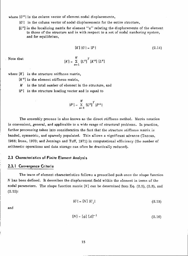
where 1U'} is the column vector of element nodal displacements,
1UI is the column vector of nodal displacements for the entire structure,
[La] is the localizing matrix for element "a" relating the displacements of the elementto those of the structure and is with respect to a set of nodal numbering system,and for equilibrium,
[K] {U I = 1P } (2.14)
Note that [ [La] [Ka] [La]a=1
where [K] is the structure stiffness matrix,
[Ka] is the element stiffness matrix,
M is the total number of element in the structure, and
{PI is the structure loading vector and is equal to
M TIPI= I [L a] {pal
a= 1
The assembly process is also known as the direct stiffness method. Matrix notation
is convenient, general, and applicable to a wide range of structural problems. In practice,
further processing takes into consideration the fact that the structure stiffness matrix is
banded, symmetric, and sparsely populated. This allows a significant advance (Tezcan,
1966; Irons, 1970; and Jennings and Tuff, 1971) in computational efficiency (the number of
arithmetic operations and data storage can often be drastically reduced).
2.3 Characteristics of Finite Element Analysis
2.3.1 Convergence Criteria
The trace of element characteristics follows a prescribed path once the shape function
N has been defined. It describes the displacement field within the element in terms of the
nodal parameters. The shape function matrix [N] can be determined from Eq. (2.1), (2.3), and
(2.12):
1U=I [N] U9e1 (2.15)
and
[N] = [c] [A]-' (2.16)
15

The shape functions are usually taken as polynomial expressions in terms of either the global
coordinates (x, y, z) or the local coordinate system (e, q, 4).The reliability of a solution by the finite element method is indicated by the fact that
the approximate numerical results come increasingly closer to the correct value as the finite
element mesh is repeatedly subdivided into finer and finer meshes (Tong and Pian, 1967 and
deAranetes, 1968).
The requirements of convergence fall into two categories: (a) completeness of the dis-
placement field U and (b) interelement continuity. First, the completeness requirement en-
sures that the energy represented by the functional (such as the integral of potential energy)
includes a constant energy state for each element. If this is satisfied, the true energy state
of the entire structure can be represented, in the limit, as the mesh layout is refined. Mathe-
matically, this requires that all uniform states of the displacement variables U must be in-
cluded in each element. This results in the equivalent requirement that "constant strain"
and "rigid body" states must be included.
The second requirement is that of continuity between adjacent elements. In order for
the functional at the element interface to remain finite, it has been considered necessary to
provide continuity of displacement variable U and its derivatives to one order lower than the
order of the highest derivative of that variable in the energy integral. The success of certain
nonconforming elements, however, has led to a reevaluation of this requirement. Bazeley et al.
(1965) suggested a less stringent condition, namely, that reduced continuity must be maintained
for the state of constant energy in the region concerned.
2.3.2 Elements of Arbitrary Shapes
Linear elasticity problems can be readily solved by a finite element technique that em-
ploys simple triangular or tetrahedral elements. The displacement fields for those elements
have often taken the form of polynomials of variables in cartesian coordinates. That is
IVuI = [0(x, Y, 3)] Iql
or
u (x,y,O)= q1 1 + q1 2 X+ q 1 3 Y+ ql4+...
v) (xya) =q 2 1 + q 2 2 x + g2 3 y + q2 4 z2 +" (2.17)
w(a,y,z) = q3 1 + q3 2 X+ q3 3 y+ q3 4 ; + " " •
In the case of the constant strain element, the criteria of convergence can be satisfied when
the assumed displacement functions 0 include the complete first order polynomial [1, x, y, z]
16

in addition to the basic requirement of compatibility* of nodal parameters. Additional nodal
variables can be introduced to give better element performance with improved representation
of the actual deformation. Selective higher order terms are to be added to ensure the continu-
ity of displacement U across the interelement boundary.
The popularity of polynomial displacement expansions 0 (x, y, z) lies in the fact that
matrix operation is straightforward and stiffness coefficients can be readily obtained in ex-plicit form by a standard procedure (see Section 2.2). It becomes obvious in application, how-
ever, that the property of a displacement variable U (x, y, z) should have no preferred directions.
This requires that the complete polynomial expansion be used in the displacement assumption.
To implement this, a simple procedure can be found to determine shape functions [N] and dis-placement patterns JU ; the tacit assumption is that matrix [A] (Eq. (2.14)) is invertible andthat the shape function is correct simply because there is a "match" between the monomialspresent in the displacement expansion and the corresponding nodal variables (Dunne, 1968).
However, this approach is not generally valid.
Complete polynomials for a compatible displacement field are well suited for the tri-
angular and tetrahedral family of elements, but the use of complete polynomial displacement
expansion may lead to algebraic difficulties in the case of arbitrary quadrilaterals, hexahedra,
and plate bending elements. On the other hand, it is possible to formulate a compatible ele-
ment that possesses rotational invariance via direct formulation by employing a coordinate
transformation (mapping) or a natural coordinate system (Irons, 1966 and Ergatoudis et al.,
1968). Additional kinematic capabilities can be incorporated by introducing intermediate nodalparameters (Zienkiewicz et al., 1971). This is another desirable feature of isoparometric
elements. A more detailed description will be given in the following chapters.
*This ensures the minimum continuity requirements of displacement at element interface.
17

CHAPTER 3
ELASTIC ANALYSIS IN THREE-DIMENSIONAL SPACE
3.1 Introduction to Solid Elements
For many years, considerable effort has been devoted to solving problems in the realm
of three-dimensional elasticity. The classical, analytical approach for solving a set of
governing differential equations derived from a three-dimensional theory is available only for
bodies with simple geometric forms and for restricted boundary conditions and limited loading
cases. Different numerical procedures (finite difference methods etc.) have been applied to
solve these differential equations; their success is generally still limited to special geometric
shapes and, at most, is of occasional academic interest. Now that the finite element method
has been eminently successful in dealing with certain complex problems such as plane stress
and plate bending, it has perhaps even greater potential for the solution of three-dimensional
problems.
The approach envisioned here is based on a full three-dimensional analysis and is com-
pletely general in nature. It will be shown that the solid elements used in the present study
are capable of correctly representing the behavior of a beam, plate, shell, or any of the varied
aspects of structural components.
Because the tetrahedron-shaped element (Fig. 3.1) has simplicity and flexibility, it
was a natural choice for the earlier development of solid elements (Gallagher et al., 1962).
The element shape is defined by four arbitrary, noncoplanar points in space. Any topography
may therefore be represented with sufficient accuracy by some assembly of these tetrahedron
elements. The drawback to this element shape is the large number of element inputs required
to describe a complex surface. The mesh is difficult to visualize, and the amount of data to
be processed as well as the number and the bandwidth of the system of equations generated
tend to exceed the storage capacity of the average size computer and call for excessive com-
puter times. To reduce these constraints, isoparametric elements, including those with a
curved face, have been introduced. These elements represent a great improvement over the
tetrahedron because they enable bodies with curved boundaries to be treated with a limited
number of elements.
3.2 The Basic Solid Element
A comparison (Clough, 1969) of the performance of solid finite elements has shown that
isoparametric hexahedron elements are distinctly superior to any tetrahedron assemblages, both
in terms of the properties of the individual elements and their application to analyze real struc-
tural systems. Isoparametric elements have the additional advantage of isotropy. It is evident,
then, that a general-purpose, three-dimensional finite element analysis program should be con-
structed around the isoparametric hexahedron element family.
19

v ", Pyj
j(xj,yj,zj)
Wi, Pzj u-,P.j
3- - (x3,y 3 ,z3 )
Y 1 ,- •
Y1 , Zl)2(x 2 ,y2,z2 )
0
z
X,Y,Z ARE GLOBAL RECTANGULAR COORDINATES
Pj Pxj A NODAL FORCE VECTOR AT NODE j
Pzj
5j= Vj A DISPLACEMENT VECTOR AT NODE j
Figure 3.1 Tetrahedron, a solid element and rectangular coordinate system
20

3.2.1 The Isoparametric Displacement Field
Consider the general family of elements with six faces, the hexahedron family. The
use of an appropriate natural coordinate system greatly simplifies the formulation of the ele-
ment stiffness matrix for some very complex members of this family. These coordinate lines
are generally curved in space and follow only the interface topology of an individual element.
As shown in Fig. 3.2 (and later in Fig. 3.3) for instance, •, •, 4 are natural coordinates; each
coordinate axis is associated with a pair of opposing faces which are given the coordinate
values of + 1. In their local reference frame, the elements take on the image of a 2 by 2 by 2
cube, whereas in the real cartesian coordinate system (x, y, z), they can be any arbitrarily
warped, six-sided solids.
We begin with the linear hexahedron that has the eight corner nodes shown in Fig. 3.2and introduce a polynomial expansion of the displacement component in rectangular cartesian
coordinates
u u (X, y, z)
=11 + q 1 2 T+ q 1 3 Y + q14 + q 1 5 Xy + q 1 6 Yz + q 1 7 zax+ q 1 8 XYz
or
u= [0,(x, y, a)] 1qjli i = 1,2 ..... , 8 (3.1)
It will be demonstrated (Section 3.2.4) that the criteria of convergence are satisfied. Without
losing generality, we can consider an element in the form of a rectangular parallelopiped with
the origin located at centroid and the coordinate planes as planes of symmetry. By evaluatingnodal displacement parameters at the appropriate coordinates, i.e., ui =u (xi, yi, as), etc., we
can assemble the nodal displacement vector, for instance, uil = [Ai.] {qi, etc. From Eq.
(2.15), we obtain by identity
u = N1 u 1 + N 2 u 2 +..... .... + N 8 u8
8= . N u. (3.2)
and1
Ni=8- (l+xix)(l+yy)(l+ Zz) i=l ..... .. ,8 (3.3)S8
wherex= + 1, y. = + 1, and zi= +1 are coordinate values at node i,
Here, Ni (x, y, z) is known as the shape function, or interpolation function, such that it takeson unit value at the indexing node (i) and is zero at all other nodes. These interpolation func-
tions are readily developed simply by writing them as the product of the equations of the linesor surfaces through all the remaining nodes. This can frequently be done by direct inspection.
21

C")
Cl))
P- C.)
ClC,
C 00
0~
NN
co,
22)

z/17
7?= 1
x CARTESIAN COORDINATES
LOCAL COORDINATES
Figure 3.3a Quadratic element (20 nodes)
r/=
t z-i -- 7
- :CARTESIAN COORDINATES
LOCAL COORDINATES
Figure 3.3b Cubic element (32 nodes)
Figure 3.3 Refined curved hexahedron
23

Proceeding in the same fashion, we can define other displacement components v and w
as
V v(x, y, z)
8
=E Nv.i=1 t
and8
w= Y Nw. i= 1, 2 ..... ., 8 (3.4)i=1 I
where the shape function Ni takes on the same form, Eq. (3.3).
As mentioned earlier, an element of prismatic shape has rather limited appeal in deal-
ing with practical problems. This geometric constraint can be relaxed by a suitable coordinate
transformation commonly known as mapping. Consider, for instance, an element of Fig. 3.2a
being distorted geometrically to a shape shown in Fig. 3.2b. In other words, map the element
into x, y, z-coordinate space such that a typical node i moves to a position (xi, yi, oi). A
relation of the forms
x= Y_ N. x.iI
y = E Niy. (3.5)
z = YN.2 i= 1, 2,... ni I
(where n = NNPE, the number of nodes per element) gives x= (, x , ), . . . and can
be used to define the mapping. Here, the shape functions
N = Ni (6, 1 7)
1= - (1 + 6:i ) (0 + 7qi r) (0 + i L) (3.6)
8
are written in terms of the local dimensionless coordinates 6, 77, and 4. Following the nodal
ordering number as given in Fig. 3.2a, we have the local nodal coordinates
(4,:, ,77, ýi):
fori= 1, 2, ... ,8
24

The displacements u, v, w can be interpolated in the same manner; hence u = u (e, 7,
etc. Again, we write
u =IN.u.
v = I N v (3.7)i
w=INi wi i=,. J..,ni
The shape functions Ni (4i, r7j, 4i) used here are identical to those employed in the coordinatedefinition and in such cases the formulation has been termed "isoparametric" (Zienkiewiczet al., 1969). With the position and the displacement of a material point in an element spacedefined, a family of isoparametric elements can be formed routinely.
3.2.2 Numerical Calculation of Stiffness Matrix
Consider an element stiffness matrix, Eq. (2.11),
[Ke] = fff [B] T[D] [B] dxdydovolume ofelement
To integrate it, we need to evaluate the integrand [B] T[D] [B] = G (X, y, z) in terms of independ-ent space variables (x, y, a). The algebraic expression of G involves the strain matrix [B]which is derived from the definition of strain and consists of appropriate first derivatives ofthe displacements. For a solid element, we have
ON.E0 0
x ax
aN.
MI.cz0 0 a2 U
)NI. MI O 1. (3.8)
Yxy ay ax 0 w
a NI. aN.Yyz 0 aO ay
aNi NI.
YX- 0 a ax i= , 2 , NNPE
= [B] tual6 x 2 4 2 4 x I forNNPE= 8
25

It is clear then the expression G is algebraicly complex and its integration presents a formid-
able task since the shape functions N, = Ni(e, -q, C) are established in local rather than global
coordinates. In order to proceed further, it is desirable to introduce an auxiliary expression
C(, ,) in terms of local coordinates (e, 7, 4).The Jacobian of the transformation is defined as J = d(x, y, z)/1(9, ,, 4) and the
matrix is
ax ay aza6 a ý aea
ax ay az -- -- -- (3.9)
ax ay az
a 1 a 2 I
a .. 4 X2
aN1 9N2 aN 8 X 3
a• a7 a 77dN 1 aN2 aN 8
a< a4 a4x 8 Y8 28
d Ni i
where - -8 (l+i 7,7) (1+4•4)ae 8
aNi (I'+ 6i )
O9 Ni cia C 8
Following the standard rule of partial differentiation, for example,
aNi aNi a Ni a• aNi a4- = + , etc.,
ax Oa Ox ,7 aOx a< ax
26

we have
aN1 aN 2 a(9 aN 1 aN 2 aN 8
aX ax ax a• a
aN 1 aN 2 aN 8 aM1 aN 2 dN8ay ay ay a (3.10)
aN 1 aN 2 an9 N3N 1 aN 2 aN8
az a2 a2 a< a< a
Now the values of aNi/ae, aN1/a17, aN9/a , and matrix [J] can be calculated point by
point in an element subregion. The matrix [B] can be readily assembled. The components of
strains everywhere within the elastic element are now defined in terms of nodal deflections
{Ua I as parameters.
The integration in terms of local coordinate variables (e, 77, C) can be executed in a
simple format, that is,
[K,] =ff G(x, y, z) dx dy dzVol
fff 1 [BI T [D] [B] IJI d dq d< (3.1t)
and
g(C7, C*) = [BIT [D] [B] IJ.(6, -q, <)I (3.12)
For all practical purposes the integration performed numerically (Hammer, 1959) as a
summation of quadratures is a simple matter on a digital computer. Here,
NPZ NPY NPX[K e l = .Y - Y- I W( ix ', 77iy ' ý j ) H x i iz( . 3[ z=l iy=l ix=l x) H. H. H.
If the Legendre-Gauss quadrature formula is employed, 6j., 7iy' (z correspond to the abscissas
for the zeros of the Legendre polynomial of degree NPX, . . . etc. NPX, NPY, NPZ are the
number of integration points to be used in each linear quadrature space. The values of ej X
and its weight factors Hix can be found in standard quadrature tables (Stroud and Secrest,
1966).
It is worth noting that the stiffness matrix [Ke] is symmetric and that the strain matrix
IB] and the elasticity matrix [D] include many zero terms, or null submatrices. A substantialreduction in arithematic operation is possible by carrying the algebraic processing a little
further. First, the strain matrix [B]
27

B 12 Bi
[]= F-(.46 x 24 [ B 2 1 B 2 2 B 2 3L_ I I
B1 0 0
0 B2 0
0 0 B3
B2 Bi 00 B3 B2
LB3 0 B1
can be expressed in terms of submatrices:
= aN1 aN 2 aN 8 ]Bt(8)=L ' a_ ) ...... ' ax
aN 1 aN 2 aN 8
B2 (8) = _ - ...... , y (3.15)8ay Jy8
aN 1 N 2 (N9B3 (8) = _ , a ......
Second, the elasticity matrix [D] which relates the stresses and strains, Eq. (2.5), can include
any anisotropic properties and can be prescribed as a function of spatial distribution, e.g.,
Di. (x, y, z). The [D] matrix is symmetric and can be written as:
wee[D (6,9 6)] = P01 100 (3.16)
where-I -ID11 D 12 D 13
[DM] = D 2 2 D23
SYM D3_.3
D44 0 07[Ds]= YM D55
[0] is a 3 by 3 null matrix. For this study, we shall consider an isotropic material. In
that case
AA BBB [D cc 0 -0
[DMl = DK AA BB [D1= DK cc
SYM A , M
28

Ewhere DK =
(1 + v) (1 - 2 v)
AA= i-v
BB= v
CC = (1 - 2 v)12E and v are the usual elastic constants, Young's modulus and Poisson's ratio, respectively.
At this stage, the calculation of element stiffness matrix can be broken into parts.
Terms that contain null factors can be screened, large number of intermediate calculations
can be eliminated, and economy in computer time can be realized. For instance:
[Ke(i,j)] = f' f 1 f 1 [B(m,i)]T[D(m,n)] [B(n,j)]IJI ded, dC (3.17)- 1 -1 __1
24x 24 24x6 6 x 6 6 x 24
or
oK(, 8) ' (r, S + 8) K(r, s + 16) 7[Ke] = K(r+8, s+8) LC(r+8, s+16) (3.18)
LSYMM K (r+ 16, s + 16)J
r, s = 1, 2. ..... . 8
A typical submatrix, for example, is
K (r,s)=f' f 1 f'[B T nD B +BT D B ]JId ejd-qd< (3.19)S- -1 M 21 s 2 1
This can be reduced to
f_.f'lf_1[Bt(r) D1 1 BI(s) + 1B2(r) D4 4 B2(s) + B3(r) D6 6 B3(s)I] IJI d6d qd< (3.20)
Other submatrices are
f 1 f 1 __[Bl(P) D 1 2 B2(s) + B2(r) D4 4 BI(s)]IJI de• d? dC
f 1 f' jl [Bl(r) D13 B3(s) + B3(r) D66 BI(s)] IJI d6 d 77 dC
Pl f EB2(r) D2 B2(s) + Bl(r) D BI(s) + B3(r) D B3(s)] IJI d/6d 7 7 d<-1 1f-1[Br 022 + 44 + 55
f-1 1 fl fl [B2(r) D2 3 B3(s) + B3(r) D 55 B2 (s)] IJI d= d? d7
f 1 f 1 [B3(r) D3 3 B3(s) + B2(r) D5 5 B2(s) + B1(r) D6 6 B1(s)] IJI d/dri d<
29

For submatrices on the diagonal, stiffness coefficients must be computed only for
those terms where s>r, since advantage is taken of the symmetry of the stiffness matrix.
Finally the nodal parameters can be regrouped, i.e.,
jUal = d
and
UUi
wi ii= 1, 2 ..... . , 8
to expedite the assembly into the entire structural system matrix [K] of Eq. (2.14).
3.2.3 Higher Order Curved Elements
In earlier developments, the boundary of a finite element was usually thought of as
composed of straight edges and its geometric form completely defined by a series of corner
nodes. Where an edge is curved, appropriate intermediate nodes must be specified along that
edge. One intermediate point will suffice to define the shape of an edge with a simple or
constant curvature. Two or more intermediate points will be required to specify the geometry
of an edge with a multiple or reversed curvature.
3.2.3.1 Quadratic Curved Element. In most cases, the boundary of a complex structuralshape can be closely represented by a sequence of quadratic curves or quadratic surfaces.
Therefore many complicated problems can be realistically defined and solved with only a
limited number of simple, discrete, curved elements. These curved elements can be readily
formulated by using isoparametric concepts (Section 3.2.1). For example, by placing one
midside node along each edge of an 8-node hexahedron, we obtain a 20-node element. This
20-node hexahedron is coming into widespread use and is an important tool in three-
dimensional analysis (Fig. 3.3a).
For a 20-node hexahedron element with edges capable of displaying simple curvatures,
we can write a displacement expansion that contains 12 terms in addition to those required
for the 8-node hexahedron (Eq. (3.1)) to ensure compatibility.
Hence,
U2 0 = [0l(X, y, z)] faiI i=1,2 ..... .. , 20
= a 1 + a 2 x + a 3 y + a4 + a 5 xy + a 6 yz + a 7 ZX + a 8 XYZ
22 2222" a9X 2 + aloy2 + allz2
"+ a1 2X 2y + a,3X2 + a 4 y 2x + al 5 y2Z + a1 6 z2 y + a1 7 2 x
"+ al X2 yz + a1 9 XY2 + a2 0 Xy2 2 (3.21)
30
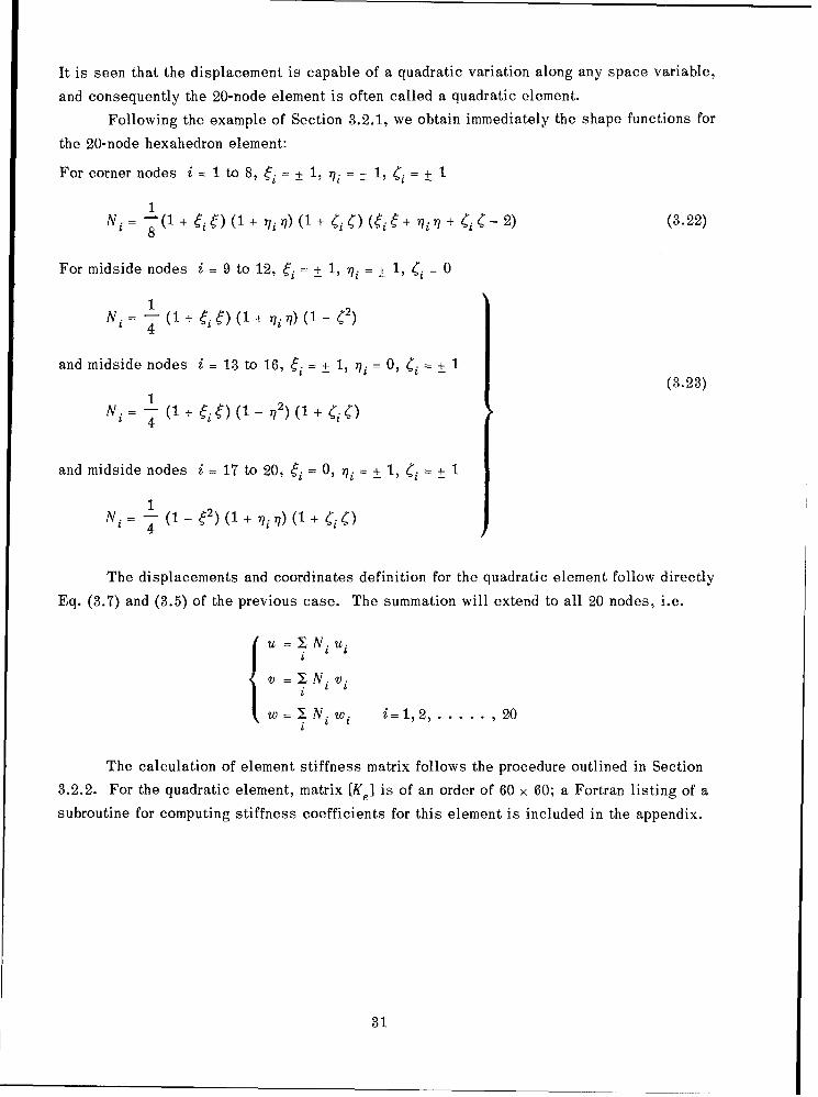
It is seen that the displacement is capable of a quadratic variation along any space variable,
and consequently the 20-node element is often called a quadratic element.
Following the example of Section 3.2.1, we obtain immediately the shape functions for
the 20-node hexahedron element:
For corner nodes i= 1 to 8, = ± 1 =+- 1, 7. + 1
1Ni = 8(1 + e=6) (1 + 7i) (1 + Ci¢) (6:i ý+ 71i 7 + CiC - 2) (3.22)
For midside nodes i= 9 to 12, •=i= ± 1, 7i= ± 1, 4 = 0
1Ni = (1 + =i e) (1 + i (1- 42)
4
and midside nodes i = 13 to 16, • = ± 1, 7i=0, 4 = + 1(3.23)
1Ni -- (I + • 4) (t - q2) (1 + 44)
4
and midside nodes i = 17 to 20, • = 0, 71=i , Ci + 1
1Ni = 4 (1 - e2) (1 + 7q 7) + Ci
The displacements and coordinates definition for the quadratic element follow directly
Eq. (3.7) and (3.5) of the previous case. The summation will extend to all 20 nodes, i.e.
u= I Niui
v { = N.v.
w= Y N w i=1,2, 20i i i ......
The calculation of element stiffness matrix follows the procedure outlined in Section
3.2.2. For the quadratic element, matrix [Ke] is of an order of 60 x 60; a Fortran listing of a
subroutine for computing stiffness coefficients for this element is included in the appendix.
31
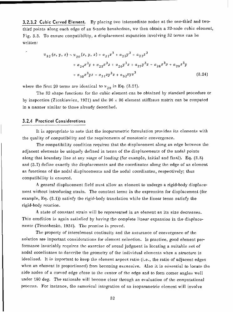
3.2.3.2 Cubic Curved Element. By placing two intermediate nodes at the one-third and two-
third points along each edge of an 8-node hexahedron, we then obtain a 32-node cubic element,
Fig. 3.3. To ensure compatibility, a displacement expansion involving 32 terms can be
written:
U 3 2 (x, y, 1) = U21(O' y, ;) + a 2 1 x3 + a 2 2 y + a 2 3 2
"+ a 2 4 X3y + a 2 5 X3 + a 2 6 y 3 + a 2 7 y 3 x + a 2 8 Z 3 X + a 2 9 3 Y
"+ a 30 X3 yz + a 3 1 Xy3 z + a 3 2 XY2 3 (3.24)
where the first 20 terms are identical to u2o in Eq. (3.21).
The 32 shape functions for the cubic element can be obtained by standard procedure or
by inspection (Zienkiewicz, 1971) and the 96 x 96 element stiffness matrix can be computed
in a manner similar to those already described.
3.2.4 Practical Considerations
It is appropriate to note that the isoparametric formulation provides its elements with
the quality of compatibility and the requirements of monotonic convergence.
The compatibility condition requires that the displacement along an edge between the
adjacent elements be uniquely defined in terms of the displacements of the nodal points
along that boundary line at any stage of loading (for example, initial and final). Eq. (3.5)
and (3.7) define exactly the displacements and the coordinates along the edge of an element
as functions of the nodal displacements and the nodal coordinates, respectively; thus
compatibility is ensured.
A general displacement field must allow an element to undergo a rigid-body displace-
ment without introducing strain. The constant terms in the expression for displacement (for
example, Eq. (3.1)) satisfy the rigid-body translation while the linear terms satisfy the
rigid-body rotation.
A state of constant strain will be represented in an element as its size decreases.
This condition is again satisfied by having the complete linear expansion in the displace-
ments (Timoshenko, 1934). The premise is proved.
The property of interelement continuity and the assurance of convergence of the
solution are important considerations for element selection. In practice, good element per-
formance invariably requires the exercise of sound judgment in locating a suitable set of
nodal coordinates to describe the geometry of the individual elements when a structure is
idealized. It is important to keep the element aspect ratio (i.e., the ratio of adjacent edges
when an element is proportioned) from becoming excessive. Also it is essential to locate the
side nodes of a curved edge close to the center of the edge and to form corner angles well
under 180 deg. The rationale will become clear through an evaluation of the computational
process. For instance, the numerical integration of an isoparametric element will involve
32

calculation of the Jacobian of the coordinate transformation, or the functional determinanta (x, y, z)
IJI I - To ensure that the mapping is unique and that there is a one to onea(6q, 0,)
correspondence of coordinates (x, y, z) and ('s, 7, 4), it is necessary that the Jacobian de-
terminant does not change sign in the element space (which implies IJI j' 0).
Now note that
ax dy a0z
ae aC a9 i 6ax dy dz T (3.25)
H an an a 7
ax a y a2a< a< a4 "
where Pe, Pq, P4 are vectors tangent to local coordinate (q, C, 4) lines (Fig. 3.4). From the
standard expression
d (Vol) = dx dy dz
= IJI dednqdC (3.26)
A Vol x yhence IJI = lim I A. Therefore, the Jacobian provides a quantitative measure by
A Vol -77
which the admissibility of an element geometry can be evaluated. This is a useful guide in
selecting the appropriate structural idealization for element application. (Since LJI = Pe •
P 4x , the Jacobian is viewed as a scalar triple product, and numerically it equals the
volume of a parallelopiped with opposing sides parallel to the vector triplet Pe, P7, P4 .)
3.3 Specialization
3.3.1 Load Matrix for a Prescribed Pressure
It is often a tedious task to calculate the load on the surface of a complex structure
due to a distributed pressure. The difficulty arises from the lack of a simple practical means
to describe a design surface. However, with the evolution associated with the isoparametric
curved element formulation, such a surface can be numerically defined and load calculation
evaluated.
In a finite element system, the layout of the element mesh pattern that represents a
structure depends on the manner in which the loads are to be carried. As a rule, loads are
prescribed only at the nodal points and in the directions corresponding to displacement com-
ponents defined in the global coordinates X, Y, and Z. Sometimes "statically equivalent"
loads are used as an expedient computation. For correct solutions especially when the
details of local stress distribution are desired, the load calculation s should follow the pro-
cedure outlined in Section 2.2.1. An example is given here.
33

CURVED ELEMENT
77 CASA
P/
ELEMENTARY AREA
zr(=P)- (,7,1
SU RFAC E
_Y
X
n = SURFACE NORMAL
Figure 3.4 Curved element representation of a complex surface
34

Consider the general case of a fluid pressure distribution
P = - q(x, y, z) , q (3.27)
where q(x, y, z) is a scalar factor that describes the variation in spatial pressure and A is the
external surface normal. In case of hydrostatic pressure, q(x, y, z) reduces to q(z). From
Eq. (2.12), the equivalent loading vector at the ith node is
I (1)j F Y N(I) IPI ds (3.28)
where N (I) is the shape function for node i and ds is the differential area of a given surface
region (D) for which the pressure has been specified.
Since the position of any point in an element body is defined by the coordinate equation
(Eq. (3.5)), points on any surface area can be readily obtained. For instance, by setting
S = ± 1, we obtain the surface equations in a parametric form for the top and the bottom faces,
respectively.
X YX N X=X(4, ij)i
Y = I N. . = Y(=, 7) (3.29)i
Z = Y- N. Z.= Z (•,77)iZ N
The summation extends to all nodes on a given surface. Nodal numbers for a given (top)
face and corresponding shape functions are shown in the following nodal number labeling scheme.
3 8 04 3 12 40
57 7 7 7 4 5 1
5 664
1 7 2 09 10 2
Quadratic Element Cubic Element
35

For the quadratic element:
Corner nodes 1, 2, 3, 4 =T1, 77i 1.1
N i = 4 ( t + 6ci 6) (1 + 77i q) (ýji + 77i7 - 1
Midside nodes 5, 6 ý, = 1, 7i= 0.1 (3.80)
N. = - (1 + 6i. 12)(( .30)
Midside nodes 7, 8 =, 0, 7i = 1.
1
For the cubic element:
Corner nodes 1, 2, 3, 4 •=¥1, 7i= 1.
1Ni= "- (1+ 6=i e) (t+ qi 77) [9 (:2 + 772)_ 0
1Side nodes 5, 6, 7, 8 77i= -- , 1 6i=l.
N.-= (I + 6i 0o (t - 17 2) (1 + 9 77i 77)332
1Side nodes 9, 10, 11, 12 3-= 3 ' 1ii=¥
9Ni = - (1- _ 2) (1 + 9 4i) (1 + 77iT)
£ 32
With the surface defined in curvilinear coordinates, i.e., S(e, -q) in Eq. (3.29), its
normal vector can be expressed by
A A A" x i + n Y + n k =P x P7 (3.32)
A .A
z kzax ay dz0
a• a a.•ae de aeax aOy a
36

where P 6 and P 77 are vectors tangent to the surface and in the directions of the 6- and -coordinate lines, respectively (Fig. 3.4). An elementary area of the surface is given by
A9 = Pe Ae x P 17 A7
The surface area of a region D is
_ lir I JP6 × P771 A6 A7
AT7 -• E
The area of one complete face of an element can be found conveniently by a numerical integra-
tion process; we have
S = f' f'1 1-i d~d77
NPT NPT (3.33)I Y I • Hi(e).Hi(77 )
i=1 =1 = . . , NPT
For a relatively smooth surface, such as the surface of a cylinder or a skewed propeller blade,
a three-point integration rule gives adequate accuracy (i.e., for NPT = 3, the error range is
0.03 to 0.12 percent). Hence the numerical integration provides an effective way to compute
a complex surface area as well as its projections and other surface characteristics.
Now the nodal load components for any node (1) due to a pressure loading on a face of
the element can be expressed as
F(I)- f f ' N(1) p} JIl d4 d 77 (3.34)
Expressed in quadrature format,
F (1) = + + ij. N (1) n.,x H n (C) .nj (77)
F (1) = I N()-n Hi H 7)(.5
F, (1) = I I qi. u (1) ,, n., H(e).nj(,7)i J
The distributed load qi] must be evaluated in a pointwise manner at each integration point
i, j = 1, 2, . . . , NPT. As before, these are the numbers of Gaussian integration points along
the e- and 77-coordinate lines, respectively. The final load vector {p} is obtained by summing
up individual contributions from all elements attached to these nodes or the network of nodes
(see Section 2.2.2).
37

3.3.2 Stresses on an Arbitrary Surface
For obvious reasons, it is conventional to give experimental stress data along certain
well-defined reference frames tangent to the surface area of interest. Expression of the stress-
es in a global coordinate system generally does not give a clear picture of the surface situation
for a structure of arbitrary shape. The stress calculation should therefore be put into a format
that allows numerical results to be readily assessed, interpreted, and/or compared to experi-
mental values or other known results.
In the process of computing stiffness coefficient matrix [K], values of strain and stress
are computed at each Gaussian quadrature point. These values are expressed in terms of nodal
displacement parameters (ui, vi, wi), with reference to the global coordinate (x, y, z) system.
As evaluated, these strain values are stored on tape. Once the equations of the structure sys-
tem are solved and nodal displacements become known, stresses and strains can be obtained by
direct substitution into Eq. (2.4) and (2.6). For design purposes, these results are sufficient
to describe the response of an elastic body in many practical applications.
For structures of complex shapes, stresses at points other than those quardrature points
may be desirable. This will require additional calculations at the designated locations where
stress evaluation is sought. Matrix [B], shown in Eq. (3.8), should be used for this purpose.
The corresponding process outlined in Section 3.2.2 must be repeated. Once again, there is a
need to define the surface orientations from which a set of local coordinates can be chosen so
that the computed stresses can be of value for immediate, meaningful interpretations.
We begin with the definition of unit normal
- (3.36)I5I
where = P6 x Pq is given in Eq. (3.32). Now let P be the unit tangent vector which isA - -
along an 71-eoordinate line and P7 = P 7P771. Then
A A
T =P 77 X (3.37)
AT will be the third unit vector, completing a right-handed orthogonal triad scribed in the body
or attached to a surface. The triad (T, P n) can be considered as a local reference frame
(x', y', a'). See Fig. 3.5 and 3.6. Hence, the matrix
^ A A ý A A
[ el, e2 e3] (3.38)
= [o0]
A Awhere P1, e 2 , e 3 are unit vectors in directions of local rectangular coordinates (x', y , 210] is also known as the direction cosines matrix. [T,, P ] can be expressed in terms of
traditional directional cosine symbols (e, m, n), namely
38

11 =COS 1 zm1 =COS f 1nI COS "/'
Y' ' ZX'nn1y
X Z,
Figure 3.5 Rotation of reference frame
i, j ...... NODAL LABEL
% 0 .... ELEMENT NUMBER1, 2, 3,.. ELEMENT NODAL
% INCIDENCE
/ 0° x
Figure 3.6 Element nodal incidence and local reference frame
39
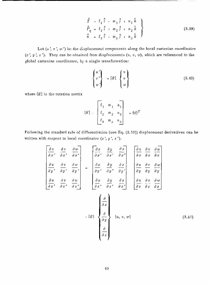
A A A AA A A A
3 +M + n2nk (3.39)S3 z + M 3) + n 3 k
Let (u', v , w ') be the displacement components along the local cartesian coordinates
(x , y ' o '). They can be obtained from displacements (u, v, w), which are referenced to the
global cartesian coordinates, by a single transformation:
V [=1 {V (3.40)
where [R] is the rotation matrix
P1 mi n][9]1 P2 M2 n2 T[]
f3 M 3n3
Following the standard rule of differentiation (see Eq. (3.10)) displacement derivatives can be
written with respect to local coordinates (x', y', z
au av aw ax ay az au av aw
ax" ax" 9x" Px" a xa a-x ax ax ax
au av aw ax ay az au av aw
ay" ayP ay" ay" ayA ay" ay ay ay
au av aw ax ay aOz au av aw
z' aoz az a' az az' aoz a az
aax
aInR] -a [u, v, w] (3.41)
ay
az
40

By substituting local displacements (u, v', w') in place of (u, v, w) in Eq. (3.41), we can
arrive at a convenient form of the expression to calculate local strain components from strains
given in global coordinates:
ax" ax" (9X"
auS' av? aw
au' av' aw'"
au aV dw
ax ax ax
a [ u dv aw [R]T (3.42)ay ay ay
au av aw
az (z az
Stress components computed in the global coordinate system can be transformed to
locally oriented stresses [a'] by a similar expression, that is,
ta'3]= H" OS *opr• r;
[R] [a] [R]T (3.43)
Once the element mesh and labeled element nodal numbers are laid out over the ideal-
ization of a structure, the element incidences must be suitably ordered (Fig. 3.6) such that
one curvilinear coordinate, 71 for instance, will be placed on a designated coordinate surface.
When the surface normal vector is computed, another orthogonal surface tangent will complete
a right-handed triad. This combination will furnish a set of local rectangular axes and form
the basis of a rotation matrix. These data enable the stresses to be calculated over an
arbitrarily shaped body along any prescribed orientation.
41
3.3.3 Applications to Plates and Shells
The solid isoparametric finite elements outlined here are based on a general three-
dimensional solution. Such elements have demonstrated broad applicability for problems in
structural mechanics. Where the element thickness is decreased to the proportion of a med-
ium thick plate (or a thin shell), a specialized formulation is permissible to achieve greater
economy and effectiveness (Ahmad et al., 1965, 1970 and Pawsey, 1970). Some well-known
approximation will be utilized in the computations of stiffness coefficients [Ke], e.g., as ad-
vocated in classical plate theory (Timoshenko and Woinowsky-Krieger, 1959 and Flugge,
1960) such that lines perpendicular to the middle surface remain straight under loading and
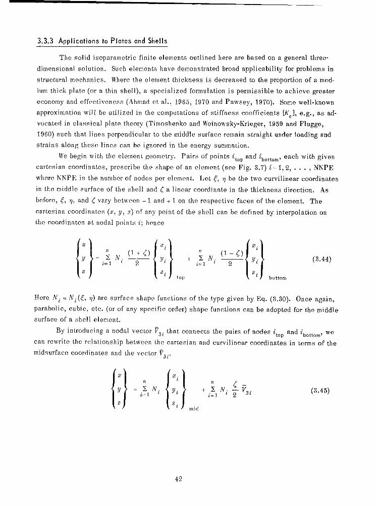
strains along these lines can be ignored in the energy summation.We begin with the element geometry. Pairs of points itop and ibottom' each with given
cartesian coordinates, prescribe the shape of an element (see Fig. 3.7) i= 1, 2, . . . , NNPEwhere NNPE is the number of nodes per element. Let ý, ý be the two curvilinear coordinates
in the middle surface of the shell and 4 a linear coordinate in the thickness direction. As
before, 6, r/, and < vary between - 1 and + 1 on the respective faces of the element. The
cartesian coordinates (x, y, z) of any point of the shell can be defined by interpolation on
the coordinates at nodal points i; hence
{ = I N + (I N bt (3.44)
top iIbottom
Here Ni = Ni( ) are surface shape functions of the type given by Eq. (3.30). Once again,
parabolic, cubic, etc. (or of any specific order) shape functions can be adopted for the middle
surface of a shell element.
By introducing a nodal vector V3i that connects the pairs of nodes itop and /bottom' we
can rewrite the relationship between the cartesian and curvilinear coordinates in terms of the
midsurface coordinates and the vector f3 .,
{§} = N Timid N1 V2 i (3.45)
422
mid
42
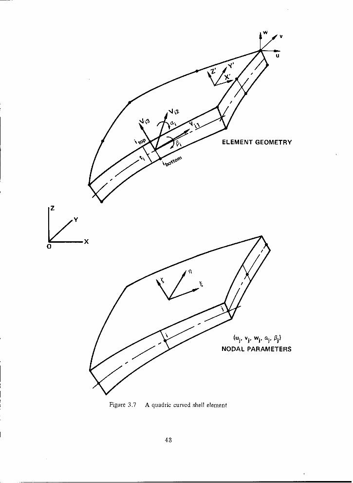
w v
ELEMENT GEOMETRY
• (ui, vj, wj, al09j)
NODAL PARAMETERS
Figure 3.7 A quadric curved shell element
43

where
v3i Yi Yi (3.46)
top- i bottom
i= 1, 2, . . . , NNPE (=n)
Now the displacement pattern has to be assumed for the element. Since the strains in
the direction normal to the midsurface are assumed to be negligible, the displacement vector
"throughout the element will be taken to be completely defined by the midsurface nodal dis-
placement Fmi and two rotations (a-, #) of the nodal normal V3i about axes orthogonal to it. IfA Atwo such orthogonal directions are given by unit vectors V2 i and VWi, with corresponding
scalor rotations ai and fpi, we can write
T= Y N. TM + C-2 (Ei + j) x f3 (3.47)
where
F= v = ui+ v+ A
w
A A A-mi Ui+ 0i + W j+ (3.48)
and
A A A
Vii = i X V3 I(A A A (3.49)V2 i = V 3 i X V 1 i
"ai = a, V2i
,} (3.50)
i = Pi vi
i=1,2, ... ,NNPE(=n)
Here u, v, and w are displacements in the directions of global x, y, and z axes, and up, vi, and
wi are displacements at the midsurface node i. At each node, we now have the five basic
degrees of freedom:
44

U.
V.ui
ai
1i
From the basic shell assumptions, the strain components are essential in directions
of tangential orthogonal axes related to the surface C = constant. The strains to be used in
the element approach must be converted to this same reference system. At a point on this
surface, take z' in the direction of surface normal T, Eq. (3.32). We can establish a set of
local orthogonal axes x', y', and z a One simple scheme is given by Eq. (3.49). The strain
components of interest are
a~u'x ax'
cav'
{ E'P= Axa = Ua + au
au, (9w'Yx 'z 1 - + -
a9' ax,
z - + -O
or
= [B'] It a (3.52)
The stresses corresponding to these strains are defined with the aid of the elasticity
matrix [D']. We have
ay
l == [D ] Ic' (3.53)
45

where
1 v 0 0 0
1 0 0 0i-v
' 0 0[D"1= - E 2 (354)
,"(l - ) 1-v 00
2 2kSYM II 1-V
2k
The 5 x 5 matrix [D '] is defined for an isotropic material. E and V are Young's modu-
lus and Poisson's ratio, respectively. The factor k (= 1.2) included in the last two shear
terms is intended to improve the shear displacement approximation (Ahmad, 1970). It is seen
that because of the displacement assumption, the shear strain is approximately constant
through the thickness, whereas in reality the shear distribution is approximately parabolic.
The value k= 1.2 is the ratio of relevant strain energies.
The next step is the calculation of the element stiffness matrix
[Kl] =f' fl f 1 [B']T [D'] [B'] J1 d6 d-q d< (3.55)-1 -1 -1
By definition, l = [B'] IUsI. Matrix [B'] relates the local displacement derivatives to the
nodal parameters. The calculation of [B'] involves three steps:
a. Compute global displacement derivatives for a set of curvilinear coordinates in the
manner shown by Eq. (3.10).
b. Transform these derivatives (i.e., the strain components expressed in global coordi-
nates) to local displacement derivatives by Ea. (3.42). Here, the direction cosine matrixA
[0] can be constructed by a process given by Eq. (3.49) with unit vector V3 parallel to z '-axis
which is in the direction of surface normal _n.
c. Assemble the local displacement derivatives to form the strain vector {e'} in terms of
nodal parameter vector [UIs given by Eq. (3.52).
Now the whole integral of Eq. (3.55) can be expressed as an explicit function of the
curvilinear coordinates. After carrying out some operations at the submatrix level, simplifi-
cations and saving in numerical processing can be achieved. A numerical integration will
allow the properties of the element to be evaluated.
46

3.4 Implementation
3.4.1 Introduction to Solution Methods
In the displacement method of finite element analysis, the problem eventually reducesto the solution of a set of linear simultaneous equations that express the load-displacementor equilibrium relation for the structure. The displacement boundary conditions can be read-ily imposed by deleting the appropriate nodal parameters (corresponding to nodal degrees offreedom) from Eq. (2.14). After reduction-which, in effect, removes the rigid-body mode-we
have
[Kr] U = P (3.56)
where [Kr] is the nonsingular structure-stiffness matrix,
U is a vector of unknown nodal parameters (displacements), andP is a vector of applied load.
Once Eq. (3.56) is solved, the global displacement parameters U become known. Thedesired stress and strain at any point within any element can be found immediately by sub-stituting the nodal displacements in Eq. (2.4) and (2.5) in turn.
In practical application, a sizable number of finite elements is required for the repre-sentation of structural design problems. Consequently, an extensive network of nodes evolvesand the size of the stiffness matrix which corresponds to the number of unknown nodal vari-ables is often overwhelming (not infrequently several thousand degrees of freedom arise). Alarge portion of the total computer time required to solve a given problem is generally con-sumed in solving the set of linear equations (Eq. (3.56)). Here, the method of solution canhave a significant bearing on the computational efficiency which is measured in terms ofdemand on core size. At times, the core requirement may dictate the applicability of thefinite element method.
It is of prime interest, then, to select a solution algorithm which takes into accountthe symmetric, positive definite and banded nature of stiffness matrix [Kr]. Further theGauss elimination is known to be numerically stable, irrespective of the order in which theequations, Eq. (3.56), are eliminated (pivot search is not necessary) and therefore the fulladvantage of symmetry can be realized. The elimination of a row S (which represents an
equilibrium equation in nodal variable Us) leads to a modification of the coefficients in theremaining rows according to the formulas
1*. _ -i. ( .. (3.57)
I I is k
4 P
47

Stiffness coefficients kip, ki (= k), • etc. represent the sum of individual element contri-
butions. It does not matter in which order the summation is made and, further, they need not
be fully summed except those in row S currently being eliminated. This process affects a
triangular array immediately below the row that is being eliminated. It can be carried out by
retaining in the core only the triangle of coefficients which moves diagonally downward as
the elimination proceeds; see Fig. 3.8.
As depicted by a coarse or a fine mesh, the finite element idealization of a structure
frequently takes the form of a simply connected region. In these cases, the stiffness matrix
can always be arranged in a nicely banded form by labeling the unknown parameters U. in a
suitable order. In the case of a closed ring that represents a multiply connected region, the
band can be large despite high sparsity. It is also true that the bandwidth of the individual
equations tends to be large in three-dimensional problems where large solid elements with
intermediate nodes along their edges are used. In addition, one has to operate on many zeroterms within the band, and this adds to the cost of solving equations by a band algorithm.
For these and many other cases as well, the "frontal" technique (see Section 3.42) requiresless storage and arithmetic than the best Gaussian banded algorithm (Melosh and Bamford,
1969 and Irons, 1970). The frontal solution algorithm is employed for this study, and is
described in the next section.
3.4.2 Frontal Technique
Most of the inefficiency in data processing keyed to matrix bandedness can be avoidedby applying the frontal technique. It is based on the principle implied by the very nature ofGauss elimination, Eq. (3.57). Frontal processing takes advantage of the fact that nonzeroelements in a column of the decomposition (inside the triangular portion of the array affected
by row operations) cannot occur in any row prior to the occurrence of a nonzero element (i.e.,the stiffness coefficient kis = k1i ý/ 0) in the column of the stiffness matrix. In this approach,
the first appearance during decomposition of an element in a column of [Kr] causes the additionof that column to the wavefront which is the "front of active variables." Data that must bereadily available on core include only the coefficients of the equations on the wavefront. Avariable becomes "active" on its first appearance and is eliminated immediately after itslast. Hence, if a variable xs is ready for elimination, there must be no subsequent elements
that contain x . (It was implied previously that ksi, ks, . . . . . , P, in Eq. (3.57) must befully summed.) Thus the size of the "front" is smaller than or, at worst, equal to the band-width of the equations. In effect, this eliminates a good number of zeroes from the process
of computation, and it saves substantially on core requirement.Fig. 3.9 illustrates an application of the wavefront method. The associated graph,
representing a portion of a ship structure, explains the name "wavefront," i.e., equation
solving is visualized as progressing like a wave over the structure. At any given time inthe analysis, the wavefront includes the total number of active degrees of freedom.
48

"+÷ + + + + + + |NLN ULL\++ ++ -+ I
+ + + + +± + + + + ROWS ALREADY BEINGPROCESSED
"+ 1+ + + + + + + +
TRIANGLE NEW-" •' L = COLUMNS
/+ +' +l +OW / + +,-++ + + ÷ +
+ -+ -+ + +
0 FRONT + +1 +
SCONTRIBUTIONS TO [Kr] + +
AFMECTED +ICONTRIUTION TOFI[K]
Figure 3.8 Stiffness matrix of a structural system (solution by the Gauss frontal technique)
49

-4' V13
123 4 5 10 11 12 1 U 13
14 Q2 2240 2 26 27 21 300 31 3 2033
21 29-4 --22 /2
34 3 36 37 CENTERLINE
0 /OF SYMMETRY
38 39 40
44 45/ 46 47
58 659 160/61 62 63 6456 5 165 6 67 68t
81; //2 S
_ 8 3 843
FRONTPROGRESSING NUMBER OF ELEMENTS = 17
NUMBER OF JOINTS = 85
LEGEND BOUNDARY NODES
• = ELEMENT NUMBER @ Ui =0
N = JOINT NUMBER ) Ui=Vi=0
Figure 3.9 Frontal processing of a finite element idealization of the cross frame of a ship
50
These are associated with partially processed degrees of freedom (or nodal variables). For
example, Fig. 3.9 shows a situation just before element ®ý) is introduced.* If there is only
one equation per joint, joints 7, 17, 27, and 60, 70, 77 (representing active nodal variables)
currently constitute the wavefront. Joints 1, 2, 3, 4, 5, 6, 14, 15, 16, 21, 22, 23, 24, and 25,
etc. (which lie to the left (back) of the dotted line) have been fully processed and are no
longer considered active. At the next step, element (D introduces the new active variables
61, 62, 71, 78, and 79. As elements are being processed one after another, the front moves
forward across the structure.
Further we observe that:
a. The order of element sequence is critical in frontal solution, just as the node numbering
is critical in a band algorithm, although the best order is not always unique.
b. Ordering of the nodes is irrelevant to the frontal technique. The node numbers are
merely unique labels that relate the degrees of freedom for element and structure. They have
no effect on the order of elimination. Here, when a given mesh is changed by adding or de-
leting nodes, the frontal data are little changed, but a band algorithm may require extensive
node renumbering in order to preserve a small bandwidth. This can be extremely valuable in
design application when a mesh is to be modified locally for a rerun.
c. The size of front and hence the storage requirements for a given problem can be
assessed from the mesh pattern such as given in Fig. 3.9. For example, before element
®•) is introduced, there are six active variables: 7, 17, 27, 60, 70, 77; immediately after
the stiffness coefficient generated by element © has been added in, the list of
active variables increases to 11.
3.5 Evaluation of Numerical Results
The preceding sections have described the formulation of solid finite elements for the
three-dimensional analysis of a general elastic body and a method for its implementation.
The performance of these elements in the representation of an elastic structure will now be
evaluated. Some preliminary computations were conducted with these elements using
examples given in Chapter 9 of Zienkiewicz (1970) and favorable numerical results were
obtained. Additional problems are included here and solutions for such basic structural
components as beams, plates, and shells are presented to verify the behavior of individual
elements and to examine the adequacy of the finite element models. A special example will
be given in Chapter 4 to demonstrate the effectiveness of the procedure in solving the
difficult problem of marine propeller blades.
*Element @ has not yet been introduced.
51

3.5.1 Prismatic Beams
3.5.1.1 A Cantilever Beam. Timoshenko (1934) treated a prismatic bar subjected to pure
bending as a problem of elasticity in three dimensions. Consider the bar bent in one of its
principal planes (x-z) by a couple M at one end and held fixed at the other. Take the origin
of the coordinates at the centroid of the cross section, i.e., point 0 (Fig. 3.10). The displace-
ment components as predicted by the theoretical solution are:
1U{ - [2 _V (x2 _ y 2)1
I?
1 M
and - = - is the curvature of the deflected bar. After deformation, points on a planeR El
cross section will remain on that plane, but the cross-sectional shape will change. The
sides of the cross section become inclined and the top and bottom edges are bent into
parabolic curves as shown by the dotted lines in Section A-A of Fig. 3.10.
An aluminum cantilever beam having a cross section of 0.5- by 0.6875-in. thick and
a length of 11.0 in. was bent by an end couple of 4.10 in.-lb. Surface displacements were
measured by using holographic interferometry (Dhir and Sikora, 1972). Three-dimensional
displacement components (u, v, w) for the top face along the front edge were obtained; seeFig. 3.10. This experiment was conducted as a preliminary process to evaluate the qualityof measurements obtainable by holography. In this case, the measured data indicate that the
beam appeared to be distorted locally near the support; the investigators had difficulty in
simulating the fixed-end condition for the slender beam.
The cantilever beam is represented by four 20-node (quadric) hexahedron elements
with a total length of 11 in. The finite element model is completely fixed at one end and
bent at the other by an end couple produced by two equal and opposite forces (=± 5.9636 lb)applied to the top and bottom midside node. Computed displacements u and v are almost
exact; they are within 0.1 percent of the correct solution. Computed stresses are good andare generally within 0.5 percent of the exact solution except at points near the concentrated
applied forces.
3.5.1.2 A Simply Supported Beam. The purpose of the current example is to assess the effectof mesh pattern (as it relates to the element aspect ratio) on the behavior of the finite ele-ment model. A simply supported rectangular beam 40 in. long and with a 0.6 by 6.0 in. cross
section is represented by four quadric elements (Table 3.1).
52

_ I I ! I-- THEORY O -
-- FINITE ELEMENT1.5-- O !/
_ V' HOLOGRAPHY O
m r"l
g£ - _
:Z: 1.0--\L)Z_ _ O U-DISPL. _
I,-,
I.U
IJJu _ O• -=. 0.5 --€/)
- C) mW-DISPL.-- 0 ,'0.0
0 2 4 6 8 10
DISPLACEMENTS ALONG THE SPAN OF BEAM (IN.)
SCANTILEVER SPAN = 11 IN. .•%7_ !
l " °X ALUMINUM BAR 11.0 X 0.5 X 0.6875 IN.
Mc = 4.10 IN.-LB
SECTION A-A
Figure 3.10 Pure bending of a prismatic bar
53

TABLE 3.1 RESULTS OF ANALYSIS OF A SIMPLY SUPPORTED BEAM
DISCRETE MODEL B1 DISCRETE MODEL B2-T 4@ • -:••'t/2
af 9t/10
K A B C D A jB C D,/4 ,,/4 £/4 £/4
LINE OF LINE OF
SUPPORT CENTER SUPPORT CENTER
OF SPAN OF SPAN
SPAN £= 40 IN. POISSON RATIO V= 0.30THICKNESS t = 6 IN. YOUNG'S MODULUS E = 30,000,000 PSIWIDTH b = 0.6 IN. BENDING STRESS a PSICENTER POINT LOAD P = 10,000 LB
Vertical Deflection Stresses at
at Section Section C
in. psi
A B C D otop Oabottom
Discrete Model B1 0.0156 0.0292 0.0390 0.0427 - 20,590 21,030
Discrete Model B2 0.0155 0.0290 0.0388 0.0425 -20,820 21,040
Beam Theory 0.0151 0.0283 0.0376 0.0412 -20,830 20,830
Theory of Elasticity 0.0158 0.0298 0.0398 0.0440 -20,720 20,890
54
These elements are of uniform size in discrete model BI while they are of nonuniform
size in discrete model B2. The beam is loaded at midspan by a concentrated force P.
Vertical deflections and normal stresses are obtained from the discrete element models. The
response of discrete model B2 with its nonuniform mesh size appears to be slightly stiffer.
Theoretical solutions (listed in Table 3.1) are obtained (a) by using elementary beam theory
in which the effect of shear stresses is neglected and (b) by elastic theory (Timoshenko 1934)
in which the beam is treated as a two-dimensional problem. Numerical results obtained by
both finite element calculations are acceptable from an engineering standpoint.
3.5.2 Plate Bending
When the thickness of an elastic body is small compared to its other dimensions, it
is called a plate. A flat plate is classified as thin or medium thick according to its span
to thickness ratio (Ut) whether, this ratio is greater or less than 40. When a medium thick
plate (5 > Ut > 40) is bent with small deflection-small in the sense that the plate deflec-
tion is small compared with its thickness-the classical plate theory (i.e., the Kirchoff
assumption) holds. Then, the laterally loaded plate can be treated as a two-dimensional
problem.
The 20-node hexahedron elements are used to model a plate structure with varying mesh
fineness (Fig. 3.11). Here the analysis is for a simply supported square plate with a 40-in.
span and a 1-in. thickness subjected to a concentrated center load. This is a severe bending
test because the situation is singular at the loading point (the solution for stresses at this
point is not bounded).
The center deflection under concentrated load obtained from finite element calcula-
tions is plotted against mesh size in Fig. 3.12. Note the rapid convergence of the deflec-
tion. For a mesh size N= 4 (Ut = 5), the calculated deflection is within 1.5 percent of the
exact solution. Numerical results for some well-known plate bending elements are also
shown in Fig. 3.12 for comparison purposes. These results are taken from the Nastran
Theoretical Manual (1969).
The dotted lines in Fig. 3.13 indicate the distribution of bending moments M. and My
along the centerline of the square plate computed from the finite element model. The theo-
retical results (Timoshenko, 1959) are for a concentrated load P applied over a circular area
of 0.05-a radius.
For general plate bending analysis, the application of the specialized element given
in Section 3.3.3 is preferred because of its efficiency and ensuing economy. Although thesolid element is not intended to be used for plate bending problems, it did behave well as a
plate when molded to the geometry of a plate. The element did yield results which converged
rapidly to the exact solution.
55

Y
Z///
0 X
a 20 IN. P = 4,000 LBt- 1 IN. E = 30,000 KSI
v = 0.30Figure 3.11a A simply supported square plate under center load
IIN=2 N=* N-
Figure 3.11b Element mesh used on the analyzed quadrant of the plate
Figure 3.11 Plate bending sample problem (example 3.1)
56
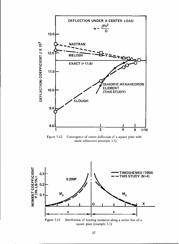
DEFLECTION UNDER A CENTER LOAD
O3Pa2
W -
D13.0
NASTRANX 1 " - , .. . ... ..
.U-- 12.0 EX T=1
zw
Q EXACT (11.6)U.W 11.0 -0
o QUADRIC HEXAHEDRON
-10.0- ELEMENTS10.(THIS STUDY)
LU
O CLOUGH
9.0 V
8.01 2 4 8 (=N)
Figure 3.12 Convergence of center deflection of a square plate withmesh refinement (example 3.1)
I-z 0.3 - TIMOSHENKO (1959)0... --- THIS STUDY (N=4)Uz 0.298P
' 0.2-0.
Z- 0.1 - x y
0 o x
Ia a
Figure 3.13 Distribution of bending moments along a center line of asquare plate (example 3.1)
57
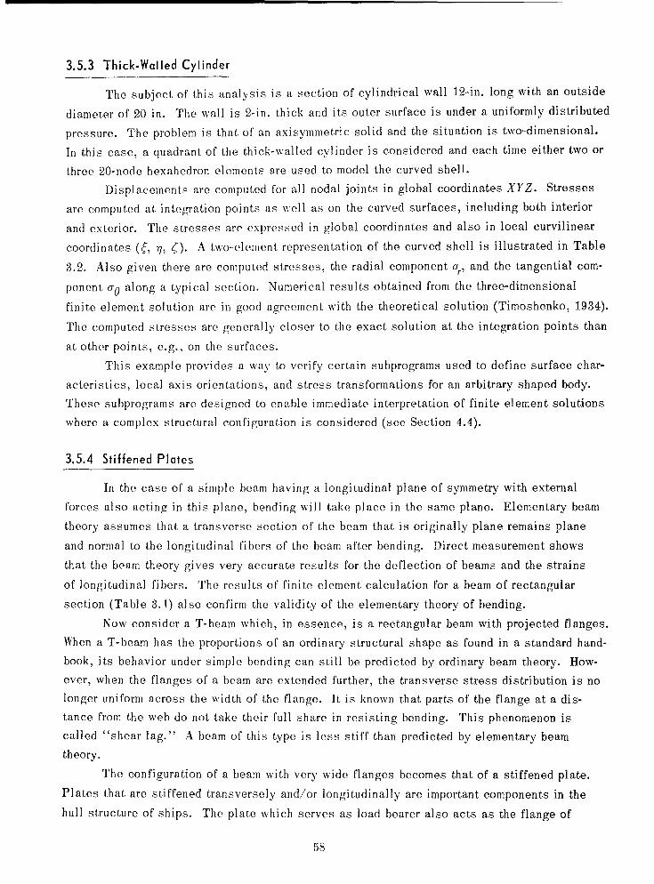
3.5.3 Thick-Walled Cylinder
The subject of this analysis is a section of cylindrical wall 12-in. long with an outside
diameter of 20 in. The wall is 2-in. thick and its outer surface is under a uniformly distributed
pressure. The problem is that of an axisymmetric solid and the situation is two-dimensional.
In this case, a quadrant of the thick-walled cylinder is considered and each time either two or
three 20-node hexahedron elements are used to model the curved shell.
Displacements are computed for all nodal joints in global coordinates XYZ. Stresses
are computed at integration points as well as on the curved surfaces, including both interior
and exterior. The stresses are expressed in global coordinates and also in local curvilinear
coordinates (C, -q, ,). A two-element representation of the curved shell is illustrated in Table
3.2. Also given there are computed stresses, the radial component ar, and the tangential com-
ponent a0 along a typical section. Numerical results obtained from the three-dimensional
finite element solution are in good agreement with the theoretical solution (Timoshenko, 1934).
The computed stresses are generally closer to the exact solution at the integration points than
at other points, e.g., on the surfaces.
This example provides a way to verify certain subprograms used to define surface char-
acteristics, local axis orientations, and stress transformations for an arbitrary shaped body.
These subprograms are designed to enable immediate interpretation of finite element solutions
where a complex structural configuration is considered (see Section 4.4).
3.5.4 Stiffened Plates
In the case of a simple beam having a longitudinal plane of symmetry with external
forces also acting in this plane, bending will take place in the same plane. Elementary beam
theory assumes that a transverse section of the beam that is originally plane remains plane
and normal to the longitudinal fibers of the beam after bending. Direct measurement shows
that the beam theory gives very accurate results for the deflection of beams and the strains
of longitudinal fibers. The results of finite element calculation for a beam of rectangular
section (Table 3.1) also confirm the validity of the elementary theory of bending.
Now consider a T-beam which, in essence, is a rectangular beam with projected flanges.
When a T-beam has the proportions of an ordinary structural shape as found in a standard hand-
book, its behavior under simple bending can still be predicted by ordinary beam theory. How-
ever, when the flanges of a beam are extended further, the transverse stress distribution is no
longer uniform across the width of the flange. It is known that parts of the flange at a dis-
tance from the web do not take their full share in resisting bending. This phenomenon is
called "shear lag." A beam of this type is less stiff than predicted by elementary beam
theory.
The configuration of a beam with very wide flanges becomes that of a stiffened plate.
Plates that are stiffened transversely and/or longitudinally are important components in the
hull structure of ships. The plate which serves as load bearer also acts as the flange of
58
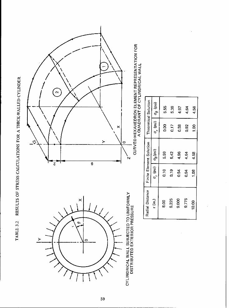
zz
0
-~ U)
x <
0- CL,)
LLr
F- F
o -J -J
F-~~~ 0 N I
Cd) Co)- L
0-c
CiuJ
-J F
59j

the stiffener. There are numerous approximate methods for analyzing these plates. Most fre-
quently, they are based on idealization of the system into a grid (or network) of beams or into
an equivalent orthotropic plate. These methods require an estimate on the effective width of
the plate and the torsional rigidity of the composite. Thus they demand considerable engi-
neering judgment and interpretation and are not completely reliable.
Important progress has been made in recent years on finite element analysis of eccen-
trically stiffened plates and shells (Mehrain, 1967; Kohnke, 1969; and Chu, 1970). The stiff-
ened plates are represented by a composite of beams and plates (one- and two-dimensional
elements, respectively). Actually, at or near the interface of the plate and its stiffener, an
accurate solution of their structural behavior would require a three-dimensional analysis.
The improved hexahedron element is utilized here to analyze the intricate stress distribution
of stiffened plates.
Fig. 3.14 indicates a general scheme used to analyze a laterally loaded stiffened plate.
The plate with a stiffener on one side is taken as a simply supported plate beam carrying a
center load P. Because of symmetry, a half span of the beam is idealized and twelve 20-node
hexahedron elements are used for its representation. At each end, vertical supports are pro-
vided for both flange and web plates. Five different flange versus stiffener aspect ratios are
used as parameters (plate beams CX2 through CX6) to assess the effect of flange width
on the structural behavior of these stiffened plates. As the flange of a beam is progressingly
widened (e.g., plate beam CX3), the maximum center deflections calculated by the finite
element representation are found to increase at a greater rate than those obtained by the
elementary beam formula. In other words, because of shear lag, each incremental flange
material is engaged in a lesser capacity than has been assumed.
Fig. 3.15 depicts the distribution of longitudinal stresses (aY) on a transverse section
of plate beam CX3. Stresses are generally higher in the parts of flange near the stiffener
and especially in the vicinity of the concentrated load. Similar patterns of stress distribution
with varying degree of stress gradient are found in each beam that has projected flanges.
Stress distribution across the web plate differs somewhat from the linear variation assumed
in the elementary theory of bending. The neutral axis at these cross sections of the beam
does not pass through the geometric centroid (Fig. 3.15). Such behavior was more pronounced
for a plate beam such as CX3 with its deeper web plate (S= 6 in.) than for the others, for
example, CX4.
Fig. 3.15 also shows the distribution of typical transverse stresses (a ) along the
flange plate. They indicate some local bending of the flange in the transverse direction near
the concentrated force. Additional stress data of interest are given in Table 3.3. These
stresses were obtained at the Gaussian integration points (used to form the stiffness matrix
of the isoparametric element). Stresses computed at such points have been shown to be
generally of high accuracy. Stresses for other locations in the plate beam can be found by
interpolation.
60

p = 10k
20-IN. 20-IN.
A SIMPLY SUPPORTED PLATE BEAM
log w
, ® ', V®_ E =30.000 KSI///_..•• __v =0.30
XZ IS THE PLANE OFZ y , SYMMETRY OF
a - _ _ _ _ _ _ _ _ _ _ _ _ P L A T E B E A M
A FINITE ELEMENT REPRESENTATION
PLATE BEAM BEAM PARAMETER CENTER DEFLECTION (IN.)
MARK w tb s ts FINITE ELEMENT BEAM THEORY
CX1 0.6 0.6 6.0 0.6 0.0425 0.0412
CX2 6.0 0.6 6.0 0.6 0.0214 0.0191
CX3 12.0 0.6 6.0 0.6 0.0185 0.0158
CX4 1.8 0.6 3.0 0.6 0.213 0.210
CX5 6.0 0.6 3.0 0.6 0.147 0.142
CX6 12.00 0.6 3.0 0.6 0.129 0.123
PARAMETERS OF BEAM CROSS SECTION AND COMPUTED DEFLECTIONS
Figure 3.14 Stiffened plate sample problem (example 3.2)
61

BW/2 W/2
- A SOLUTION
2-0 Y -- FINITE ELEMENTcc 'SOLUTION
-1.0 - a X a" y
0.0_ _ NEUTRAL
oCENTERLINE oo,BEAM SECTION AT OF BEAMY 0.676 IN.
-5.o- 10.0 5.0 0.0 -5.0Uj y(KS I)
S-1.0oIax_, - .
NEUTRALAXIS 7/ ý
CENTERLINE/BEAM SECTION AT OF BEAM SY =3.00 IN. ay
,-5.o
S-1.0 _ a x _ 0.
NEUTRALAXIS
I CENTERLINEBEAM SECTION AT OF BEAM SY = 9.50 IN. I
STRESSES ON FLANGE PLATE STRESSES ON WEB PLATE CL
Figure 3.15 Distribution of normal stresses in a plate beam (example 3.2)
62

TABLE 3.3 LONGITUDINAL STRESSES (a y) IN A STIFFENED PLATE (EXAMPLE 3.2)
'Table 3.3a Plate beam CX2
y _y , (psi)
(in.) A1 A2 A3 B1 B2 B3 Cl C2 C3
0.676 -6252 -5103 -3479 - 6795 -5417 -3525 -7768 -6215 - 41273.000 -5989 -4945 -3529 - 5845 -4817 -3450 -5959 -5000 - 37555.324 -5557 -4471 -3074 - 5267 -4442 -3411 -5063 -4555 - 39619.500 -3683 -3180 -2547 - 3725 -3201 -2537 -3748 -3199 - 2498
16.500 -1155 - 979 - 752 - 1214 -1039 - 814 -1255 -1082 - 863
D1 D2 D3 E1 E2 E3 F1 F2 F3
0.676 -9161 -6841 -4624 -10247 -7926 -5705 -2533 5995 181933.000 -6093 -5051 -4045 - 6575 -5528 -4519 -2225 5486 164205.324 -4773 -4496 -4048 - 4646 -4367 -3916 -2135 4687 142659.500 -3757 -3232 -2466 - 3639 -3113 -2347 -1126 3541 9634
16.500 -1200 -1050 - 854 - 1230 -1079 - 882 - 387 1203 3182
a a b _b I_ a a2 - 2 2 b =0.6 IN.2 1 = 0.3873
Bb c =S-bA aB C Ec S-
4! H I .0? I0
u• ~~ABOUT eL " -|
7
23 C,
F
w w
2 2
POSITION OF INTEGRATION POINTS USED IN STRESS TABULATION
63

Table 3.3b Plate beam CX3
y oay (psi)
(in.) A1 A2 A3 B1 B2 B3 Cl C2 C3
0.676 -3267 -2335 -1374 -3979 -2855 -1713 -5092 -3791 - 24803.000 -3428 -2378 -1311 -3487 -2511 -1531 -3878 -2995 - 21195.324 -3454 -2267 -1076 -3158 -2311 -1473 -3124 -2641 - 21779.500 -2015 -1629 -1244 -2151 -1717 -1283 -2268 -1803 - 1338
16.500 - 522 - 369 - 218 - 729 - 586 - 444 - 805 - 670 - 537
D1 D2 D3 E1 E2 E3 F1 F2 F3
0.676 -6733 -4610 -2802 -7851 -5731 -3925 -1290 +5261 140953.000 -4173 -3260 -2491 -4656 -3745 -2980 -1004 4775 12740
5.324 -2771 --2668 -2541 -2619 -2519 -2393 -1045 4024 11155
9.500 -2265 -1872 -1455 -2130 -1736 -1317 - 299 3157 760516.500 - 713 - 587 - 445 - 747 - 621 - 479 - 84 1107 2505
Table 3.3c Plate beam CX4
y a y (psi)
(in.) Al A2 A3 B1 B2 B3 Cl C2 C3
0.676 -48270 -37590 -26240 -48610 -37800 -26415 -49440 -38595 -272553.000 -43650 -34230 -24500 -43315 -33880 -24220 -43200 -33840 -243305.324 -39980 -30840 -21740 -40005 -30960 -22030 -39965 -31100 -224359.500 -21720 -21230 -15420 -27150 -21320 -15550 -27130 -21340 -15590
16.500 - 9105 - 7235 - 5325 - 9110 - 7207 - 5277 - 9160 - 7225 - 5270
D1 D2 D3 El E2 E3 F1 F2 F3
0.676 -50570 -38710 -27930 -51640 -39780 -29005 -12830 +28290 70310
3.000 -43655 -33720 -24340 -44135 -34210 -24830 -11605 25560 635205.324 -39870 -31220 -22580 -39765 -31120 -22490 -10430 22850 568309.500 -26980 -21315 -15520 -26860 -21195 -15400 - 7100 16000 38930
16.500 - 9136 - 7210 - 5315 - 9162 - 7236 - 5343 - 2400 5389 13220
64
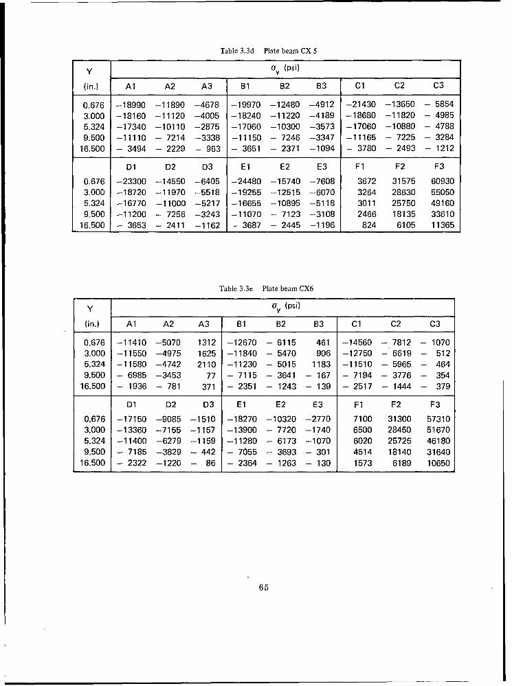
Table 3.3d Plate beam CX 5
y aOy (psi)
(in.) A1 ,A2 A3 B1 B2 B3 Cl C2 C3
0.676 -18990 -11890 -4678 -19970 -12480 -4912 -21430 -13650 - 5854
3.000 -18160 -11120 -4005 -18240 -11220 -4189 -18680 -11820 - 49855.324 -17340 -10110 -2875 -17060 -10300 -3573 -17060 -10880 - 47889.500 -11110 - 7214 -3338 -11150 - 7246 -3347 -11165 - 7225 - 3284
16.500 - 3494 - 2229 - 963 - 3651 - 2371 -1094 - 3780 - 2493 - 1212
D1 D2 D3 E1 E2 E3 F1 F2 F3
0,676 -23300 -14550 -6405 -24480 -15740 -7608 3672 31575 609303,000 -18720 -11970 -5518 -19255 -12515 -6070 3264 28630 550505.324 -16770 -11000 -5217 -16655 -10895 -5118 3011 25750 491609.500 -11200 - 7256 -3243 -11070 - 7123 -3108 2466 18135 33610
16.500 - 3653 - 2411 -1162 - 3687 - 2445 -1196 824 6105 11365
Table 3.3e Plate beam CX6
y Oy (psi)
(in.) A1 A2 A3 B1 B2 B3 Cl C2 C3
0.676 -11410 -5070 1312 -12670 - 6115 461 -14560 - 7812 - 10703.000 -11550 -4975 1625 -11840 - 5470 906 -12750 - 6619 - 512
5.324 -11580 -4742 2110 -11230 - 5015 1183 -11510 - 5965 - 4649.500 - 6985 -3453 77 - 7115 - 3641 - 167 - 7194 - 3776 - 354
16.500 - 1936 - 781 371 - 2351 - 1243 - 139 - 2517 - 1444 - 379
D1 D2 D3 E1 E2 E3 F1 F2 F3
0.676 -17150 -9085 -1510 -18270 -10320 -2770 7100 31300 573103.000 -13360 -7155 -1157 -13900 - 7720 -1740 6500 28450 51670
5.324 -11400 -6279 -1159 -11280 - 6173 -1070 6020 25725 461809.500 - 7185 -3829 - 442 - 7055 - 3693 - 301 4514 18140 31640
16.500 - 2322 -1220 - 86 - 2364 - 1263 - 130 1573 6189 10650
65

CHAPTER 4
SPECIAL CLASS OF STRUCTURAL PROBLEMS
4.1 Introduction to Propeller Blades
Marine propeller blades present a special class of structural problems for which no
generally satisfactory solution is presently available.
Screw propellers have been and remain the principal device used to move a ship.
Despite their importance, there is little or no realistic approach by means of which an accu-
rate evaluation of propeller stresses can be obtained. The problem lies in the difficulty of
describing a blade design in simple mathematical terms. Until recently, existing methods ap-
plicable to screw propellers have relied heavily on practical experience and semitheoretical
considerations. They provide a criterion of stress rather than the actual surface stresses.
In the past, analytical methods for predicting blade stresses have been developed by
using "beam" theory or "shell" theory. The use of elementary beam theory was first pro-
posed by Taylor (1933) who treated a blade as a cantilever attached to the propeller hub and
recommended that stresses be calculated for cylindrical blade sections with the neutral axis
parallel to the nose-to-tail (pitch) line* of the expanded section. Cantiliver beam theories
have yielded reasonable estimates of stresses at certain selected points of relatively straight
and narrow blades. Some modified forms of beam theory have been proposed (Rosengh, 1937;
Hancock, 1942; Schoenherr, 1963; and McCarthy and Brock, 1969) for wide-bladed propellers
with blade width to length ratios of about 1. The shell theory approach was first proposed by
Cohen (1955) who treated a simplified propeller blade model as a helicoidal shell with vari-
able thickness and infinite width. However, where this approach was applied to the problem
of a shell of finite width, it was impossible to produce a solution to satisfy the boundary con-
ditions. Later studies included those of Conolly (1961) and others (General Applied Science
Laboratory, 1963 and Atkinson, 1968). Shell-type theories that incorporate broad assumptions
do not appear to offer tangible improvement; moreover, they are rather involved for routine de-
sign purposes. Analytical methods that attempt to predict blade stresses on the basis of
conventional mechanics have not been eminently successful.
Considerable effects have been devoted to measuring blade strains on both model and
prototype propeller blades (Connolly, 1961; Wereldsma, 1965; McCarthy and Brock, 1969;
and Boswell, 1969). In certain cases, good agreement was obtained between beam theory
and measured data. However because of the large number of factors involved, care must be
taken in drawing general conclusions from limited measurements.
*See Comstock (1967) for propeller terminology.
67
The trend in shipbuilding to full afterbodies for mammoth tankers and bulk carriers and
to higher speeds for modern naval vessels has been accompanied by large irregularities and
fluctuations in the wakes of such ships. As a result, the propeller experiences increased dy-
namic excitation and generates severe vibratory forces on the hull and propulsion system.
Propeller-induced vibration is one of the main problems associated with ship propul-
sion employing the screw propeller. The thrust derived from blade-lift force is unsteady
when the blades rotate in a nonuniform velocity field behind the ship. The interaction of
these unsteady forces with the hull and appendages causes the excitation of the ship by the
propellers. Blade skew, high blade area ratios (i.e., wider blades), and a larger number of
blades per shaft have all been tried in an attempt to reduce vibration. These innovations of
propeller geometry drastically alter blade displacement patterns (Dhir and Sikora, 1971, 1972)
and render the standard methods (i.e., beam theory) invalid. If blade design is to have a
sound and rational basis, then an effective analytical method is clearly required so that suit-
able blade strength and stiffness can be determined for a specified ship-operation task.0
The finite element procedure outlined in Chapter 3 will now be used to analyze a
screw propeller in its more general form, that of a highly skewed propeller. The computed
results will then be compared with measured displacements and stresses derived from mea-
sured strain under steady pressure loading. This study will provide the basis for further ex-
tending the procedure until it is eventually able to take unsteady stressing due to dynamic
effects and fatigue behavior into account.
4.2 The Geometry of Skewed Propellers
When properly designed, skewed propeller can be used not only to significantly reduce
propeller-induced vibrations but also to improve blade performance against cavitation, etc.
(Cummings et al., 1972).
The general characteristics of screw propellers and their typical design process can
be found in standard sources (Comstock, 1967). A propeller is usually described by a set of
architectural drawings that show various views of the blade and a table that gives detailed
dimensions of blade sections including pitch angles, camber ordinates, thickness ordinates,
and chord lengths. These are useful input for propeller manufacturers. Application of the
finite element procedure, however, requires analytical specification of the blade geometry,
i.e., the definition of a suitable set of coordinate systems.
The highly skewed propeller is a recent innovation and its geometry is more involved.
The skewed blade illustrated conceptually in Fig. 4.1 is shown in Fig. 4.2 as a projection on
the XY plane. Two right-handed coordinate systems share the common Z (= 2) axis (coincid-
ing with the centerline of the shaft). The common Z-axis is taken positive downstream from
the propeller. One of the systems is the global rectangular coordinates (X, Y, Z), a ship-fixed
frame of reference whose origin lies on the shaft centerline at a convenient longitudinal
68

w a,x
z co UJ l-
wUC d2 JII -
wP Z0
0U-c LIU
00
0l Zw 0 L
00
0
o 4O)
z~
0 0~0 z LLJ
w< LUa-r Z
I- .L
z Uj 69
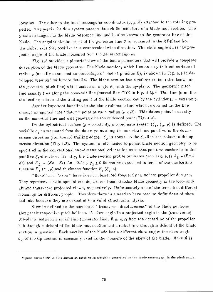
location. The other is the local rectangular coordinates (x,y, Z) attached to the rotating pro-
peller. The y-axis for this system passes through the midchord of a blade root section. The
y-axis is tangent to the blade reference line and is also known as the generator line of the
blade. The angular displacement of the generator line 0 is measured in the XY-plane from
the global axis OX, positive in a counterclockwise direction. The skew angle 0S is the pro-
jected angle of the blade measured from the generator line oy.
Fig. 4.3 provides a pictorial view of the basic parameters that will provide a complete
description of the blade geometry. The blade section, which lies on a cylindrical surface of
radius p (usually expressed as percentage of blade tip radius R), is shown in Fig. 4.4 in de-
veloped view and with more details. The blade section has a reference line (also known as
the geometric pitch line) which makes an angle b P with the xy-plane. The geometric pitch
line usually lies along the nose-tail line (curved line CDE in Fig. 4.3).* This line joins the
the leading point and the trailing point of the blade section cut by the cylinder (p = constant).
Another important baseline is the blade reference line which is defined as the line
through an approximate "datum" point at each radius (p _< H). This datum point is usually
on the nose-tail line and will generally be the midchord point (Fig. 4.4).
On the cylindrical surface (p = constant), a coordinate system (61, •2, p) is defined. The
variable ý, is measured from the datum point along the nose-tail line positive in the down-
stream direction (i.e. toward trailing edge). 62 is normal to the ý 1 -line and points in the up-
stream direction (Fig. 4.3). The system is left-handed to permit blade section geometry to be
specified in the conventional two-dimensional orientation such that positive camber is in the
positive 2 2-direction. Finally, the blade-section profile ordinates (see Fig. 4.4) EU = (Ec +
Et) and EL = (Ec - Et) for -0.5c < 61 < 0.5c can be expressed in terms of the camberline
function E, (6, p) and thickness function Et (61, p).
"Rake" and "skew" have been implemented frequently in modern propeller designs.
They represent certain specialized departures from orthodox blade geometry in the fore- and-
aft and transverse projected views, respectively. Unfortunately use of the terms has different
meanings for different people. Therefore there is a need to have precise definitions of skew
and rake because they are essential to a valid structural analysis.
Skew is defined as the sucessive "transverse displacement" of the blade sections
along their respective pitch helices. A skew angle is a projected angle in the (transverse)
XY-plane between a radial line (generator line, Fig. 4.2) from the centerline of the propeller
hub through midehord of the blade root section and a radial line through midchord of the blade
section in question. Each section of the blade has a different skew angle; the skew angle
0. of the tip section is commonly used as the measure of the skew of the blade. Rake fR is
*Space curve CDE is also known as pitch helix which is generated as the blade rotates; Op is the pitch angle.
70

6?(p) = RAKEes(p) = SKEW ANGLE
p (p) = PITCH ANGLE N. OUTLINE OF
OUTLINE OF 0000,"
CY LEADBLA
I\ /'! FOR VIEW A-A
SX O ; / SEE FIGURE 4.4
/ DIS DATUM POINT
LINE CDE IS THE NOSE-TAIL LINE LOCATED ON A CYLINDRICAL SURFACE OF RADIUS p(THE BLADE IS CUT BY A CYLINDRICAL SURFACE CONCENTRIC TO THE PROPELLER AXIS, LOOKING AFT)
Figure 4.3 Local blade coordinate system (x, y, Z) and (p, 0, Z)
71
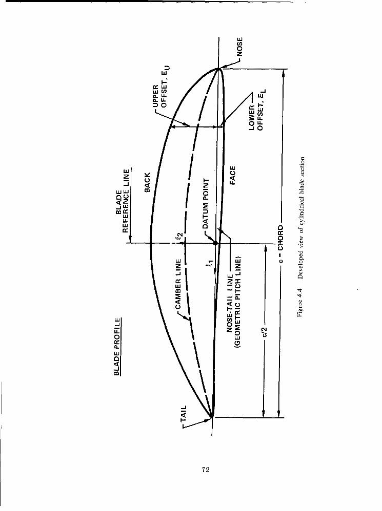
0z
-u-
0uLJO
C0CIVLU
z-j g z h
4Z
_JLU 2z lzwL I 0
0
LU wz zIU LU
I--LUL
0-0
0LU
72
defined as the successive longitudinal "displacement" forward or aft of the blade sections
from the radial reference line (Fig. 4.3). These definitions of rake and the skew allow the
datum points along a blade reference line to be described analytically by (p, O(p), 5R (p)) with
respect to the local cylindrical coordinates (p,• 0, s). Hence the blade section profile and
complete blade surface can be constructed.
4.3 Experimental Data
Dhir and Sikora (1971) used holographic interferometry to predict the static deflections
of a highly skewed marine propeller blade model. The aluminum blade model (Fig. 4.5) was
loaded on one side by a specially designed pressure chamber under controlled air pressure
(Boswell, 1969 and McCarthy and Brock, 1969). Applied pressure ranged from 0.032 to 0.192
psi. This holographic technique uses laser as the light source and is capable of measuring
the displacement components of complex surfaces witha resolution of about i0 J in.
The three-dimensional displacements were derived from fringe patterns formed in the
holographic interferogram (Fig. 4.6). The interferometric fringes on an object were related to
optical path differences, and the double exposure technique was used in its formation (in this
case, air pressure was applied to the blade after the first exposure was made). Dark and light
fringes represent contours of constant spatial blade displacements. As the applied pressure
increases on the propeller blade, the fringe pattern remains essentially unchanged but the
number of interference lines increases. The appropriate displacement components can be ex-
pressed as a linear combination of the "number" of fringes. This number is counted from the
(fixed) hub to the point of interest (obtained through certain designated observation points on0
the hologram plate) and is multiplied by the wavelength of light used (A = 5145 'A; see Dhir and
Sikora (1971, 1972) for a detailed description). Refined displacement data are obtained by
applying the least-square approximation technique.
The fringe pattern of the hologram indicates that the contours of constant displacement
line cross the circular lines which correspond to blade sections of constant radii at various
angles. It is concluded that the deflections of the blade do not follow those predicted by the
conventional method based on "beam" theory.
Strain measurements on a highly skewed model propeller blade were first made by Boswell
(1969). The blade model of 2014 aluminum was similar to that shown in Fig. 4.5 except that it
had a skew of 120 deg. Strain-gage rosettes were placed along cylindrical blade sections, five
each at the 30-, 50-, and 70-percent radii and three at the 90-percent radius. The rosettes were
so oriented that both tangential and radial strains were measured. For every gage located on the
blade face, there was a corresponding gage on the blade back.
The blade was subjected to air pressure loading by using the technique described
previously. The strain distribution was found to be radically different from that pteviously
measured on unskewed blades. The high principal stresses occurred in a relatively narrow
band which extended from near the trailing edge at the blade root to near the leading edge
at the 90-percent radius.
73

Figure 4.5 Aluminum blade model (looking forward)
Figure 4.6 Interferometric fringe patterns of blade model with applied pressure (= 0.098 psi)
74

To obtain an experimental assessment of the effect of skew on blade stress distribu-
tions, Cumming et al. (1972) conducted further tests on a series of one-blade versions of pro-
pellers with various degrees of skew. These propellers were made of the same material and
tested under the same loading conditions. Stress data for a blade with 72-deg skew were ob-
tained for comparison with the present study.
4.4 Finite Element Analyses
The three-dimensional curved elements described in Chapter 3 are used here to predict
static deflections and stresses for a highly skewed propeller blade. The blade model is sub-
jected to a uniformly distributed pressure applied on its back surface, and its root section is
assumed to be completely fixed. This loading is not the anticipated service load distribution
but was selected to match the experimental conditions. Nonuniform loading represents noproblem to the program and the influence of load distribution on stresses can be investigated.
The propeller blade used in the current analysis is one in a series of skewed, researchmodel propellers that form part of a larger study undertaken to determine the blade strength
and other performance characteristics of highly skewed propellers. Each propeller consists
of five equally spaced 1/23-scale propeller blade models attached to a cylindrical hub (Fig.
4.7). The version selected for this study (Fig. 4.5) is a single-blade model of 2014 aluminum
with a tip radius of 6 in. and a skew angle of 72 deg.
The geometry of the propeller blade has been shown to be rather involved (Section 4.2).
Application of the finite element method requires precise coordinate definition of hundreds of
discrete points that cover the complete top and bottom surfaces of the blade. A sizable effort
is therefore involved in the calculation of coordinate data. Existing computer programs, e.g.,Brockett (1972), and other data generation routines are designed to furnish the pertinent geo-metric description of a propeller blade. Nevertheless it is the responsibility of the user to
discern the validity of his input.
The coordinate data for this analysis were obtained from the geometric output generatedby a numerical machine* from input of blade section parameters. As seen from its plotted pro-
jection (Fig. 4.8), the coordinate data are for a blade situated in a position 144 deg ahead ofthe blade shown on Fig. 4.2. The geometric data have been checked visually and by graphical
means; however, rigorous error analysis has not been attempted.
Discrete point locations on the blade surfaces were chosen for the element mesh net-
work. Figure 4.9 shows that these points were along 20-, 30-, 40-, 50-, 60-, 70-, 80-, and
90-percent blade radius, etc. They are those points for which blade section geometries were
given and for which displacement as well as strain measurements were made. It is only natural
that these points are adopted in the formation of the element mesh.
*A numerically controlled machine used for model cutting.
75

UNSKEWED BLADE HIGHLY SKEWED BLADE
Figure 4.7 Projected view of two 5-bladed model propellers (model propeller series, part I)
76

C) LL
zz
C.)
o to
z
w 3
0cc-
770

Y
LEGEND
0 X ELEMENT NUMBER
SHAFT -,; ELEMENT NODE
AXIS
HUBINTERFACETRAILING EDGE-,,
LEADING EDGE
Figure 4.9 Curved solid element representation of a 72-degree skewed propeller blade
78

Three elements were used to span the chordwise dimension, and four elements were
used to cross from the blade root to its tip. Available coordinate data and element shapes
into which the blade was discretized were taken into consideration. This arrangement
allowed a direct comparison of computed and measured deflections and immediate interpre-
tation of the stress calculation.
To a large extent, the effectiveness of a finite element analysis depends on the appro-
priate element arrangement or mesh pattern which is used to represent a given structure. The
maximum number of elements is generally dictated by considerations of accuracy and cost.
The accuracy of the computed results increases as the number of elements increases, pro-
vided the resulting elements are not so numerous as to exceed computer size limitation or the
number of computations are so large that round-off errors become a dominant factor. On the
other hand, as the number of elements increases, the cost of input preparation and computa-
tion processing also increases. Obviously a compromise is required for these two competing
considerations. There is no easy way to attain an optimal mesh; nevertheless, numerical in-
stability or distortion of element performance can always be avoided by the discreet exercise
of good engineering judgment. (Some basic rules for element mesh layout were described in
Section 3.2.4.)
After element meshes were generated and nodes labeled, the elements were numbered
in succession such that the maximum front width (see Section 3.4.2) was optimized. In the
finite element method, each element is defined by a series of nodes to which it is connected
and its orientation (with reference to local axes) is determined by the numbering sequence of
the nodes defined in the incidence table. The first two numbered nodes serve to fix the
direction of element axis-6. The element axis-n is taken in the direction of a line from the
first to the third numbered node. The 4-axis is obviously the remainder that completes the
right-handed element axis system. In the case of propeller blades, nodes can be placed along
a cylindrical surface so that the direction of local element axes 6 and q will respectively
correspond to the radial and tangential axes of the cylindrical coordinates.
Note that the experimentally determined blade displacements were measured with re-
spect to the global coordinates (X, Y, Z) when the blade was oriented in the position shown
in Fig. 4.2, where 01 = 124.96 deg. The finite elements coordinates obtained from the numer-
ical machine provided a blade with the projection shown in Fig. 4.9, i.e., 01 was approximate-
ly 269 deg. Finite element calculations gave displacement components u and v that were 144
deg out of phase (A0 1) with reference to measured displacements; accordingly, the element
displacements were transformed so that they could be compared on the same scale (Fig. 4.10).
Computed displacements were obtained along the cylindrical blade section at 30-, 40-,
50-, 60-, 70-, 80-, and 90-percent radii in addition to points near the blade tip. Measured de-
flections by holographic interferometry are available at 50-, 70-, and 90-percent radii on blade
face; these are plotted on Fig. 4.10.
79

Cl) wJD z
Uf) 0 9-
I. w
2/0 CI-w
S0 0 C 10
L) CC c
0r0
/f 09-
01 I J a
1' Li
C.) L:
'I) CC 9
.) 0 (W1.o 0
6 dr* .
z I80

INCH X 10-3 50 PERCENT RADIUS
1.5 I
0.5
0.0 0.25 0.50 0.75 1.00FRACTION OF CHORD
70 PERCENT RADIUS5.0 I i I I I I I
4.0
3.0
2.01-
1.0
0.01I
T.E. L.E.
90 PERCENT RADIUS5.0I I I
F.0
8.0120--<- HOLOGRAPHY
---- FLAT SHELL ELEMENT1. -CURVED SOLID ELEMENT
0.01 I I I IT.E. L.E.
Figure 4.10c Displacement W
81

Computed stresses in global coordinates at interior points as well as surface points
are given along cylindrical blade sections. Stress outputs are available at 30-, 50-, 70-, and
90-percent radii and at many intermediate points. Stress transformation is applied so that
there is an option to print out stresses in local cylindrical coordinates. Stresses in most
areas are obtainable by interpolation. Computed stresses are plotted on Fig. 4.11 together
with stresses calculated from experimentally obtained strain data.
4.5 Discussion of Results
Fig. 4.10 shows that blade displacement component w (parallel to the centerline of the
propeller shaft) was generally higher near the trailing edge than near the leading edge for
various blade radii. This was also visible from the interferometric fringes (Fig. 4.6) repre-senting displacement contours. This indicates that displacements for a skewed propeller areno longer parallel to the cylindrical blade sections. Clearly this is a case for which theassumption made by the conventional method of blade design is not valid. Further it is notedthat the values for u and v are appreciably larger than the displacements that can be account-ed for by beam theory. A new approach is needed to predict the elastic behavior of a skewed
blade.
Genalis (1972) treated the skewed blade as a thin shell and idealized it as an assem-blage of discrete, flat, triangular elements; see Fig. 4.12. Because of the complexity of bladeprofiles and blade surface curvatures (such as described previously in Figs. 4.3 and 4.7), alarge number (about 270) of these shell elements is required in order to achieve a reasonableapproximation to the geometry of a skewed blade. Thus a substantial effort is required forinput preparations including all coordinates and load data. (It is conceivable here that thechance for input error is increased because of the huge amount of complex input data involved.)Furthermore, the proportions of the elements in the region near the hub are well beyond thelimits of medium thick plate or thin shell theory from which such elements are derived. Com-puted displacements were given for the shell solution along cylindrical sections at 50- and70-percent radii (Fig. 4.10).* The discrepancy of the numerical results as obtained from theflat thin shell element solution, from the isoparametric finite element, and from the experi-mental methods can be attributed (a) to the geometric mismatch introduced by using a flatshell element approximation for this highly curved blade of varying thickness and (b) to thebreakdown in the suitability of thin shell theory in the region near the hub. (Furthermore,some inaccuracy may be attributable to rounding errors developed during the solution process.)The error accumulation evident in the thin shell element values at the 70-percent radius waseven more pronounced at 9 0-percent radius.
*Any inaccuracy of input data will almost inevitably show up in the numerical results. The reliability of com-puted values may be increased if an appropriate algorithm is available to screen or to smooth input. The toler-ance in the fabrication of the blade model was said to be within 5 percent.
82

0 z
0 0c0 z0 wf
In 0W - 0 10 m 0Con WiLL 0 LU 0 U 00
.z uW 0 4<1 40 4 L w.
-cn U.. - 4etU ui c 0 0 0
cc ~mLL 0 o
0 z
WWO 0 W 75
LoI 0- '- z Ccc0
C~rL =I 0in LC) 1CL~1
~ LL.... 1 - W L...L... L..LID
cc
0
o o _ n
ao 00
40 0 0 0
C; z40L 0 0c w
00 0 Lu L Co0 ) 0 0 a 0 <0cc~ ~ ~ 0 <w t,< L
w z04 0 c 0040U. Z ; 0 X ) L
0.. 000 0 'q o wo 0-
00) 0i CLzc
cc4nc 0 WLL. 0 0 u 0
0 Co
0 04
0 0 0(n
CLL
N N -e * N4 N q* N1 N O
83

w
w
0 a
-o
-o
0
F-C
84

The changing profiles of the successive sections from blade root to tip indicate that
the skewed blade has a more complicated geometry than an ordinary shell. The blade is
treated in this study as a solid continuum of general shape. It is represented by 12 curved,three-dimensional elements which are capable of fitting smoothly in any complex surface.
Use of these isoparametric elements gives a marked improvement in the numerical results(Fig. 4.10). Note that the computed displacements agree well with holographic measurements,especially in displacement component w, which is by far the dominant factor of the total blade
displacement.
The largest disagreement between the displacements, which are solved for directly bythe two procedures (experimental and isoparametric finite element) is in the horizontal dis-
placement normal to the shaft axis. Possible causes for such a discrepancy might be slippageof the test specimen at the support bolts in the hub and mismatch of the isoparametric propel-ler surface with that of the test specimen. However, since the differences do not show up inthe other displacements, the latter explanation seems unlikely. Furthermore, support slippage(i.e., a difference between the ideal clamped condition of the finite element method and thefixity achieved in the test) also seems unlikely because of the low pressures involved. Ifmovement did occur, it would have to be rigid-body movement normal to the axis of the shaftrather than the more likely rotation or tipping. The final possibilities are errors in readingand/or possible binding of the blade model on the pressure seal.
The stress distribution of highly skewed propellers is expected to be unsymmetric anddifferent from that of an unskewed blade. The maximum radial and tangential stresses arelocated away from midchord and toward the trailing edge in the main body of the skewed blade.The magnitude and distribution of stresses along the cylindrical chords of the blade varieswith blade skew. Computed stresses were obtained from the same element mesh (Fig. 4.8)and were shown together with experimental stresses in Fig. 4.11. No calculated stress was
given by the shell element program (Genalis, 1972).A finer mesh would have given a closer approximation to the true stress distribution
since convergence is assured with the compatible elements used in the current study.In some of the experiments, difficulties were encountered in providing a precise fit be-
tween the test pressure chamber and the propeller blade; thus free movement of the blade edgewas not always obtained. (It was also noticed in the course of stress evaluation for a seriesof test propellers with varying degree of skews that maximum stresses and blade skews did notincrease in direct proportion.) It is desirable therefore to implement a comprehensive test pro-gram to enhance the reliability of experimental results. The stress agreement shown in Fig.4.11 was much better on the back or loaded face than on the front face, and the agreement wasbetter for tangential than for the radial stress. However, since the stresses are one step re-moved from direct measurement the agreement is not out of line even with these differences.
Since the near tip region of the blade is a sensitive region, a higher density of elements in that
85
region seems desirable. Coupled with the comprehensive test program, this should assist in
resolving the differences and provide an accurate delineation of the stresses.
The present procedure can generate an estimated complete stress field for the propel-
ler and thus provide a detailed account of the stress distribution throughout the elastic body.
This is of great practical value for a structure of unconventional configuration where conven-
tional methods offer little guidance as to the pattern of stress distribution for a structure
like a skewed propeller. A development that utilizes three-dimensional curved elements is
probably the most effective analytical method currently available and is capable of represent-
ing both the complex blade geometry and load distributions with ease and validity.
86

CHAPTER 5
CONCLUSIONS AND RECOMMENDATIONS
The rational approach established herein represents the first step in a general solution
of the propeller strength problem. A finite element displacement model is utilized to predict
the behavior of an elastic body of arbitrary shape under static loads. Compatible solid ele-
ments in their general form are adopted. This formulation bypasses the constraints of simpli-
fying assumptions and allows a closer approximation to the true structural configuration than
is possible by most other approaches, for instance, by classical plate or shell theories. Solu-
tions are subsequently obtained for displacements and internal stresses.
The numerical results obtained by the refined curved elements described in Chapter 3
are distinctly superior to those obtainable with commonly available simple triangular or rec-
tangular finite elements. The displacements obtained for a complex structure under prescribed
loading had a good degree of precision even with the relatively coarse mesh employed. This
study confirms the findings of Clough (1969), Zienkiewicz (1971), etc. that significant improve-
ments in element performance are obtainable when higher order displacement functions are em-
ployed in the element formulation.
For structures loaded so that a steep stress gradient prevails, stress predictions can
always be improved by using progressingly finer element meshes. The element presented in
this study showed a rapid rate of convergence as the mesh was refined.
The mapping technique, which is based on the application of the shape function as de-
scribed in Chapter 3, provides an expedient way to describe the geometry of a general continu-
ous surface. Load computations for a prescribed pressure distribution are therefore conducted
in a routine manner.
The method developed in this study is particularly valuable to structures with arbitrary
configurations such as skewed or unsymmetric geometry. Large savings in labor and comput-
ing costs are possible when the flat-plate or shell-element representation of a complex skewed
body is replaced by curved elements. The present development offers perhaps the only real-
istic solution available for many difficult structural problems of a three-dimensional nature,
such as a highly skewed propeller. The method now permits rapid solutions for structures
with varying degrees of skew, camber, and loading.
Among other significant applications, the present procedure can provide stress calcula-
tions at the root section of a propeller blade joining the hub, at the complicated intersection
of cylindrical walls such as a piping joint, and at the delicate interface area of a sandwich
construction. Further extension of the analysis may include considerations of anisotropic
material properties as well as the nonlinear or plastic behavior of materials (Gupta, 1971).
The current method provides a general and realistic solution to the structural problem
of a propeller under static loads, and eventually a procedure can be evolved for the complete
87

solution of propeller strength under all possible service loads. Inasmuch as a propeller
blade experiences varying vibratory forces in addition to the "nearly steady" thrust that is
always present during ship operation, a dynamic analysis that includes an investigation of
fatigue behavior of the complex ship component is naturally of prime significance.
It is recommended that the current procedure be extended to incorporate a mass matrix
of the propeller blade and an auxiliary matrix to account for the effect of "added mass" of
the fluid medium surrounding the blade. When a pressure-time relation for a propeller is pre-
scribed, a complete dynamic response can be obtained by using a time increment numerical
technique. The effect of damping may also be incorporated.
A sound propeller design is extremely important to the successful operation of a ship
and has a significant bearing on its performance. It is worth noting that improved design
methods including a dynamic analysis are being vigorously pursued by Norwegian and
Japanese ship builders. To remain competitive, U.S. ship builders must take advantage of
new technologies and be instrumental in their development.
88

ACKNOWLEDGMENT
The author expresses his thanks to staff members of the Department of Civil Engineer-
ing and of the Department of Computer Science at the University of Illinois, Urbana-Champaign,
for helpful discussions throughout the course of the investigation. In particular, he is in-
debted to Dr. W. Schnobrich under whose direction the doctoral dissertation was prepared.
Messrs S. Bakhrebah and K. Hirchert were of invaluable help in the development of the com-
putational algorithm.
The Advanced Ship Division of the Department of Structural Mechanics, NSRDC, pro-
vided the funding for the study. Members of the Propulsor Technology Branch (Code 1544)
and the Advanced Ship Division (Code 173) offered useful experimental information on propel-
ler strength. The author is grateful to Messrs A. B. Stavovy and R. G. Allen and to
Dr. J. C. Adamchak for their continued interest and support.
89

APPENDIX
EXAMPLE OF FORTRAN PROGRAM FOR NUMERICAL CALCULATIONOF AN ELEMENT STIFFNESS MATRIX
An outline of the process is described in Section 3.2.2.
91

LISTSU~rýOJT INE ST 1FFR( XY Z ,E NU, cK)COMMON /VAB7/ INTGLRND,NPTNPTS,NPZ
COMMON~ /BLAV/GM(3,5),PX(3),PY(3),Oo SUr3ROUTINF TO CALCULATE THC STIFFNESS MATRIX SK FOR ISO-PARAMETRICCC SK=INTEGRAL PHI DVC WHEFE PHI= B T X 1) X BCC X.. 0..0.... =VLCTOR OF PARTIALS OF NCI)C 0 ... Y ... 0.. WITH RESPECT TO XC 13= i... 0... Z... Y ... =VECTOR OF PARTIALS OF N(I)C Yoo. X.60 0. .. WITH RESPECT TO YC il.. 2 ... Y... Z ... =VcCTOR OF PARTlALS OF N(I)C Z ... a.*. X... WITH RESPECT TO ZC 0 ... =. VECTORC NOTE. THAT THIS MATRIX MULTIPLICAT ION HAS BEEN DON 7ALGEBRAICALLY
C PRIOR TO COOING.C
* REAL CHI(20,3),CHIX(2U),GHIY(214),CHIZ(2J)EQUIVALENCE (CHIXCI),CHI(l,1)),(CHIYUl),CHI( 1,2)),CCHIZ(1),CHI(1,3
X))REAL JAC (3,3) ,DTJJ11 ,J1.,J13,J21,J22,J23,J31,J32,J33
X,J21),(JAC(2,2),J22),(JAC(2,3),J23),(JAC(3,l),J31),(JAC(3,2),J32),X (JAC (3,3), J33)DIM:NSION EK(bU,6fi) ,SK(606,u) ,XYZ (20,3)DINENSION A(36),Hi(36),ISWK(bUu),TZ(3,,3),S(i3)
c EQUIVAL.ENCES AnOVE AP~E LOGlGALLY NECESSARYC EQUIVALENCES BELOW A;kE USEEC ONLY TC CONSERVE SPACE'
XXXF1) , (S(ý) ,SIYYP1) ,(3(6) ,S2YYP1) ,(S(7) ,S2ZZPi) ,(S(7) ,S3ZZPI) ,(S( 8
X) ,U S') , (S ( 116) , CON)CC GAUSSIAN OUAIJRATURE CONSTANTS
DAlA A/I *0.0.030 uiUbUu IJu(1, -0i.57735 02691 8963, 0.57735 U2691. 8953,3-0.?7 -t59 66.ý92 4+148, C0.U(;UJu j~2L J30jJ1 C.77q59 66692 '+148,4-0*86113 63115 94>3, -0.33993 lj435 8486, 0.33996 1J435 8485,4~ ).66113 u3115 94-5, -0.9-b17 36'+ý9 3866, -.- 53846 931ul 585 0.00000 00000 0011, U.53846 93101 0568, 0.9U617 93459 .386b,6-3.93246 95142 u 315, u.61393864 6627, -5.23851i 91863 8323,6 J.23361 91361 83230, u.66121 93864 6627, C.9324b 961'+2 U315,7-3*94'310 79123 427o, -3, 74153 118:ý5 9 91349 , -U.40584 5 1 t13 771401,7 0.06300 uo UO otO, 0.4u-L584 51513 774~U, 0.7415ý3 11855 9939,7 6.9491L 79123 4276, -[.9L-,,28 956'-'L 9754, -i,.79o0'6 64774 1363,8-u.62553 241-99 !633, -0.1e,343 -t6424 9565, 6.18343 46,+24 9505,8 3.52553 243-99 1633, '0.79bo6f 047 7 4 136j, IJ.96W28 98564 9754/DATA H/
1 2 .3G~ 0303a323, ýi 1..3 c 0 V6.8 c.u .w jU6 3 u3 J.5-3555 55555 5 15 6, u .6ýý6 66888 6 18 9, u . 5 55 5565 ý 5 5556,4 .3 47 85 '+6+51 3745, .C. 6 ý2 1,+ 515'8 6 2 i5 , u . 6ý21. 451348 6255,4 U .34785ý 4a4+51 3745, 0.23u92 6i850 5619, U.,+7862 86704 9937,5 3'.t6886s 8888B 6689, C.H,78u2 861.4 9937, u.23o692 b8850 5619,6 Li.17132 44923 7917, Z. 36ý76 15732 ~+81.4, ~.t713-3345 7269,
6 .46791 393'+5 7 2 E9 s 0. 3b. ' 1573u 4814, U0.17 132 4 + 92 7917,7 l. 12 34 8 49661 b 887, U .2797u 63914 6923, 0. 38163 00 56 5 06312,7 C.41795 91836 7347, C.36183 035 5 12, u.2797,0 53914 8928,
7 .12948 496o1 ud67, 3. 1r122 653. '33, 22238 10344 5337,
8 0. 3 13 7 6 66458 7789, 0.3t8268 37833 7836, 0.36268 37833 7836,8 0.31370 b6,+'5 8 7789, 0. 22233 10344 53337, 0.10U122 85362 9038/
C SIZE CONSTANTS
92
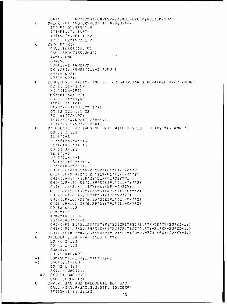
Ut'ill NprN/2J/,LNPTSf/4,KSIZE/6J/,KSIZ,,Mf/,9/C CHK-CK APT ANJ COýýPCT IF NLGESSARY
IF(:IJPT.*GT. 8)NPTz bIF (NPT.LT.1)NPT=1I? IzNPT* (NPT-1)/2IPZ- '4PZ*iNr2Z-I) 12
C ZE.ýC' MATRIXCALL ZLý.OZ(Grl,li)CALL ZLrPZ(SK,3t6JC)
NPZ1: NPZ4-1NDýZ2= NF'Z+2
C LOOFS OVER) XX,YY, ANDJ ZZ FUR GAUSSIAN r2UADRATURE OVER VOLUMEDO 21 IXX=1,NPTXX=A (IXX+IPT.)HXX=H( IXX+IPT)DO 23- LYY=1,NPTYYAý (I YY4.IPT)FiXX'lYY=H <X*H ( IYY +IPT)DO 22 IZZ=l,NPZ2ZZ= A(IZZi-IPZ)IF (iZZ.EQ.NPZI) ZZ=-1.0"IF(IZZ.cE'bNPZ'2) ZZ=1.0
C CALCULAITE HARTIALS OF NCI) WITH RESPECT TO XX, YY, AND ZZ
S1=2 *1 -'-7S1XXP I = SI*XX+ I .SIYYPI=SI*YYUl.00 3 3 J = It2
JP=2*(J-1.) +-i2YY?2 1zS2*YY+l.
S? Z7P.I=S24 ZZ#-1 .CHIlX(JP+0)=S1*U.2E*SYYPI*(I.-ZZ**2)C- Y ( JP +ý) =S2 * . 25*S IXXP 1*(I.*- ZZ* *2)CHiZ T JF-+e) =-j.5*ZZ*SXXPJ*S2yyplCd1 7X (J) 2 ) =S14 5.25*S2ZZPI*(I.-YY**2)C'i1y (JP+i2) -l-fl *yy*SIXXPI*S2ZZPICHI1Z(JP+'2)=S20j.25*S1XXP1*Ci.-YY**2)CH ix (J P+ 1.6) =- Q 5*x *XXS1YYPI*S2ZZPCriIY (JP+1ý>)=SI %,. 25*S2ZZPI*(i.-XX**2)CHIZ(JP+ý)=S2*tJ.254SiYYPI*(1.-XX**2)0O 3J K= , 2S 3=2*<- -'KP=4*CK-i) +.JPSSZZPl=S3*ZL+1.CHIX (KPI):SI * ý3125S2YYP1*S3ZZPI*( S1'2. XX 'S2*YY*S 3*ZZ-1.)CH1y (KE) :'ý2%* 12 5SI XXP1*S3ZZP1 (S2*2. 'YYi+SI*XX'S3*ZZ-1.)
30 CHIZ(K<P)=S3*0.122'*SlXXP1'*S2YYPI4 (S3*2.*ZZ+Sl*XX+S2*YY-i.)C CALCULATE JAC:PA`TIALS X XYZ
DO 4: =-
SUM=U. (L00 41 K=1,t4PTS
41 SJM=SJM !+CAI (K,I) *XYZ(K,J)4G JAC(I,J)=S:SU
DO 42 L1, 3PX (L)= JAC (1,L)
42 PY(L)= JAC(2,L)CALL SURF.N(TZ)
C INVERT JAG AND CALCULATE DLET JAGCALL :lINVDP(JAC,3,23,OE-TJ,IO,IEXP)IF(ID-i) 31,31,33 9

91 FORA4AT (1X,110,*TH ORDER PRONCIPAL MINOR IS ZERO*
STOP31 CONT INU E
C CALCULATE PATIALS WITH RESPECT TO X, Y, AND Z FROM PARTIALS WITHC RESPECT TO XX, YY, AND ZZ BYC NEW.PARTIALS=JAC INVERSE X OLD.PARTIALS
0O 50 11I,NPTS
CHIYI=CHIX (I)
CHIZI=CHIZ (1)CHIX (I) =J11#CHIXI14J12*CHIYI*Jt3*CHIZICHIY(I)=J214CHIXI+J22*CH.IYIiJ23*U'HIZI
50 CHIZ(I)=J31*CHIXI4-J32*CHIYI+J33'*CHIZI
IF(IZZ.GT.NPZ) GO TO 22
C CALCULATE. INTEGRATION CONSTANTCOt4=DE TJ*DK*HXXH YY*H (IZZ +IPT)
C DO SUMMATION FOR HALF OF MATRIX00 6U I=1,NPTSX1=CHIX (I)YI=CHIY (I)Z1=CHIZ (I)00 60 J1,NPTSX2=CHIX (J)Y2=CHIY (J)Z2=CHIZ (J)SK(I,J+NPTS)=SK(I,J*NPTS)+CON*(23B*X1#Y2+CC#Y1*X2)SKIJLPS=KIJLPS)CN(BX*2-CZ*2SK(I+N1PTS,J+LNPTS)=SKCIi+NPTS,J+LNPTS)+CON#(BB*Yi*Z2+CC*Zi*Y2)IF(J.LT.I) GD TO 61X2=X I*X 2Y2=Y1*Y2Z2=Zi* Z2SK(I,J)=SK(I,J)tCON*(AA*X2+CC*(Y24-Z2))SK(I4,NPTS,JtN4PTS)=SK(I+NPTSJ+NPTS)+CON*(AA*Y2+CC*(X2+Z2))SK(I*LNPTS,J+LNPTS)=SK(I4+LNPTS,J+LNPTS)*CON*(AA*Z2s.CC*(X2*Y2))
61 CONTINUE60 CONTINUE
22 CONTINUECALL GLOAD (XX,YY,HXXHYY,XYZ)
20 CONTINUERETURNEND0
94

REFERENCES
The following initialisms are used in the list of references:
AIAA American Institute of Aeronautics and Astronautics
ASCE American Society of Civil Engineers
IUTAM International Union of Theoretical and Applied Mechanics
NSRDC Naval Ship Research and Development Center
RINA Royal Institute of Naval Architecture
SNAME Society of Naval Architects and Marine Engineers
TAPIR Technical University of Norway
WPAFB Wright-Patterson Air Force Base
Abrahamsen, E., "Structural Design Analysis of Large Ships," Trans., SNAME (1970).
Adamchak, J. C., "User's Manual for the Modified Finite Element Program FINEL,"
NSRDC Report 3609 (Nov 1970).
Ahmad, S. et al., "Curved Thick Shell and Membrane Elements with Particular Reference
to Axisymmetric Problems," Proc. Conference on Matrix Methods in Structural Mechanics,
Air Force Institute of Technology, WPAFB (Oct 1965).
Ahmad, S. et al., "Analysis of Thick and Thin Shell Structures by Curved Finite Ele-
ments," Int. J. Num. Meth. Eng., Vol. 2 (1970).
Araldsen, P. 0. and 0. Egeland, "General Description of SESAM-69 (Super Element
Structural Analysis Modules) European Shipbuilding Vol. No. 2 (1971).
Arantes e Oliveira, E. R., "Theoretical Foundations of the Finite Element Method,"
Int. J. of Solids and Structures, Vol. 4, pp. 929-952 (1968). See also later comments by
B. M. Irons et al., in this Journal; Vol. 6, pp. 695-697 (1970).
Argyris, J. H., "Energy Theorems and Structural Analysis, Part I, General Theory,"
Aircraft Engineering Vol. 26 (Oct-Nov 1954) and Vol. 27 (Feb-May 1955).
Argyris, J. H., "Continua and Discontinue," Proc., Conference on Matrix Methods in
Structural Mechanics, WPAFB (Oct 1965).
Atkinson, P., "On the Choice of Method for the Calculation of Stress in Marine Pro-
pellers," Trans. RINA (1968).
Bazeley, G. P. et al., "Triangular Elements in Bending-Conforming and Nonconforming
Solutions," Proc., Conference on Matrix Methods in Structural Mechanics, WPAFB (Oct 1965).
Boswell, R. J., "Static Stress Measurements on a Highly Skewed Propeller Blade,"
NSRDC Report 3247 (Dec 1969).
Brockett, T. E., "Propeller Perturbation Problem," NSRDC Report 3880 (Oct 1972).
Chu, T. C. and W. C. Schnobrich, "Finite Element Analysis of Translational Shells,"
University of Illinois, Civil Engineering Studies, SRS 368 (1970).
95

Clough, R. W., "Comparisons of Three-Dimensional Finite Elements," Conference on the
Application of Finite Element Methods in Civil Engineering, Vanderbilt University; Proc.
published by ASCE (1969).
Cohen, J. W., "On Stress Calculations in Helicoidal Shells and Propeller Blades," Neth-
erlands Research Center TNO for Shipbuilding and Navigation, Delft, Report 21S (Jul 1955).
Comstock, J. P. (Editor), "Principles of Naval Architecture," SNAME, New York, N. Y.
(1967).
Conolly, J. E., "Strength of Propellers," Trans. RINA, Vol. 10 (1961).
Courant, R., "Variational Methods for the Solution of Problems of Equilibrium and Vi-
bration," Bull. Am. Math. Soc., Vol. 49 (1943).
Cox, G. G. and W. B. Morgan, "The Use of Theory in Propeller Design," Meeting of
Chesapeake Section, SNAME (Feb 1972).
Cumming, R. A. et al., "Highly Skewed Propellers," Trans. SNAME (1972).
Dainora, J., "An Evaluation of the STARDYNE Systems," ONR Symposium on Numerical
and Computer Methods in Structural Mechanics, Urbana, Illinois (Sep 1971).
Dhir, S. K. and J. P. Sikora, "Holographic Displacement Measurements on a Highly
Skewed Propeller Blade," NSRDC Report 3680 (Aug 197t).
Dhir, S. K. and J. P. Sikora, "Holographic Analysis of a General Displacement Field,"
Proc. of Symposium on the Engineering Application of Holography, Los Angeles (16 Feb
1972).
Dunne, P. C., "Complete Polynomial Displacement Fields for the Finite Element Method,"
J. Roy. Aeron. Soc. Vol. 72, pp. 245-246 (1968). See also comments by B. M. Irons et al.,
on pp. 709-711 of that issue.
Ergatoudis, J. et al., "Curved, Isoparametric, Quadrilateral Elements for Finite Element
Analysis," Int. J. Solids and Structures, Vol. 4 (1968).
Felippa, C. A., "Refined Finite Element Analysis of Linear and Nonlinear Two-
Dimensional Structures," Univ. of Calif., Berkeley, UCSEL Report 66-22 (1966).
Flugge, W., "Stresses in Shell," Springer-Verlag, Berlin (1960).
Fraeijs deVeubeke, B., "Upper and Lower Bounds in Matrix Structural Analysis,"
AGARD-ograph 72, Pergamon Press (1964).
Gallagher, R. H., "Large-Scale Computer Programs for Structural Analysis," ASME
Annual Winter Meeting, New York City (Nov 1970).
Gallagher, R. H. et al., "Stress Analysis of Heated Complex Shapes," J. Aerospace
Sc. (1962).
96

Genalis, P., "Structures Department Status Report on Propeller Strength Research,"
NSRDC Technical Note SD 730-229 (1972).
General Applied Science Laboratory, Inc., "Propeller Blade Vibration and Stress Analysis
Program," Westbury, N. Y. (June 1963).
Gupta, A. K. et al., "Elasto-Plastic Analysis of Three-Dimensional Structures Using the
Isoparametric Element," University of Illinois, CE Studies, SRS 381 (1971).
Hammer, P. C., "Numerical Evaluation of Multiple Integrals," in "On Numerical Approxi-
mation," edited by R. E. Langer, The University of Wisconsin Press, Madison (1959).
Hancock, N., "Blade Thickness of Wide-Bladed Propellers," Trans. INA Vol. 83 (1942).
Hartung, R. F., "An Assessment of Current Capability for Computer Analysis of Shell
Structures," WPAFB, AFFDL-TR-70 (Feb 1970).
Herrmann, L. R., "Finite Element Bending Analysis of Plates," Proc. ASCE Vol. 93,
EM5 (1967).
Hrenikoff, A., "Solution of Problems in Elasticity by the Framework Method," J. Appl.
Mech. Vol. 8 (1941).
International Ship Structures Committee, "ISD/ISSC Symposium on Finite Element Tech-
niques," edited by M. Sorensen, University of Stuttgart (Jun 1969).
Irons, B. M., "Engineering Application of Numerical Integration in Stiffness Method,"
J. AIAA (1966).
Irons, B. M., "A Frontal Solution Program for Finite Element Analysis," Int. J. Num.
Meth. Eng. No. 2 (1970).
Irons, B. M. and K. J. Draper, "Inadequacy of Nodal Connections in a Stiffness Solution
for Plate Bending," J. AIAA 3.5 (1965).
Jennings, A. and A. D. Tuff, "A Direct Method for the Solution of Large Sparse Symmet-
ric Simultaneous Equations," in "Large Sparse Sets of Linear Equations," edited by J. K.
Reid, Academic Press (1971).
Kamel, H. A. et al., "An Automated Approach to Ship Structure Analysis," Trans.
SNAME Vol. 77 (1969).
Kohnke, P. C. and W. C. Schnobrich, "A Finite Element Analysis of Eccentrically Stiff-
ened Circular Cylindrical Shells," University of Illinois, CE Studies, SRS 351 (1969).
Langefors, B., "Theory of Aircraft Structure Analysis," Zeitschrift fur Flugwissenschaf-
ten Vol. 6 (Oct 1958).
Logcher, R. D. and C. M. Sturman, "STRUDL-A Computer System for Structural Design,"
J. Struct. Div. ASCE Vol. 92 (Dec 1966).
97

Ma, J. H., "Elastic Analysis of a Midship Compartment by the Finite Element Method,"
NSRDC Technical Note SML 131 (Apr 1969).
MacNeal, R. H. and G. W. McCormick, "The NASTRAN Computer Program for Structural
Analysis," The MacNeal-Schwendler Corporation (1967).
Mallett, R. H. and S. Jordan, "MAGIC An Automated General Purpose System for Struc-
tural Analysis: Engineers' Manual," WPAFB AFFDL TR-68-56 (Jan 1969).
McCarthy, J. H. and J. S. Brock, "Static Stresses in Wide-Bladed Propellers," NSRDC
Report 3182 (Sep 1969).
Mehrain, M., "Finite Element Analysis of Skew Composite Plate," Ph. D. Thesis,
University of California, Berkeley (1967).
Melosh, R. J., "Basis of Derivation of Matrices for the Direct Stiffness Method," J.
AIAA (Jul 1963).
Melosh, R. J. et al., "Efficient Solution of Load-Deflection Equations," J. Struct. Div.
ASCE ST 4 pp. 661-676 (1969). See also comments in later issues of this Journal: J. S.
Campbell et al., ST 12 (1969); V. B. Venkayya and B. M. Irons, ST 1 (1970); S. S. Tezcan I
et al., ST 2 (1970); S. Klein, ST 5 (1970); and Closure in ST 2 (1971).
Melosh, R. J. et al., "Structural Analysis and Matrix Interpretive Systems (SAMIS)- Pro-
gram Report," Jet Propulsion Laboratory TM 33-307 (Dec 1966).
Moe, J. and A. Tonnesen, "Model Experiments and Finite Element Analysis of Stress in
an Open Ship," European Shipbuilding Vol. XV (1966).
National Aeronautics and Space Administration, "The NASTRAN Theoretical Manual,"
edited by R. H. MacNeal, NASA SP-221 (Oct 1969).
Paulling, J. R., "The Analysis of Complex Ship Structures by the Finite Element Tech-
nique," J. Ship Res. (Dec 1964).
Pawsey, S. F., "The Analysis of Moderately Thick to Thin Shells by the Finite Element
Method'" University of California, Berkeley Civil Engineering Department SESM Report 70-12
(1970).
Przemieniecki, J. S. et al., "Proceedings of Conferences on Matrix Method in Structural
Mechanics," WPAFB (1965, 1968, 1971).
Roren, E. M. Q., "Finite Element Analysis of Ship Structures," in "Finite Element
Methods in Stress Analysis," edited by Holand and Bell, TAPIR, Trondheim, Norway (1969).
Rosingh, W. H. C. E., "Design and Strength Calculations for Heavily Loaded Propellers,"
Schip en Werf (1937).
Schoenherr, K. E., "Formulation of Propeller Blade Strength," Trans. SNAME, Vol. 71
(1963).
98
Schrem, E., "Computer Implementation of the Finite Element Procedure," "ONR Sympo-
sium on Numerical and Computer Methods in Structural Mechanics," University of Illinois.
Urbana (Sep 1971).
Schrem, E. and J. Roy, "An Automatic System for Kinematic Analysis, ASKA," IUTAM
Symposium on High Speed Computing of Elastic Structures, Universite De Liege, Belgium
(1971),
Stroud, A. H. and D. Secrest, "Gaussian Quadrature Formulas." Prentice-Hall, Engle-
wood Cliffs (1966).
Taylor, D. W., "The Speed and Power of Ships," Ransdell, Inc., Washington, D. C. (1933).
Tezcan, S. S., "Computer Analysis of Plane and Space Structure," J. Structure Div.
ASCE Vol. 92 (1966).
Timoshenko, S., "Theory of Elasticity," McGraw-Hill Book Company, New York. NY
(19 34)0
Timoshenko, S. and S. Woinowsky-Krieger, "Theory of Plates and Shells," Second
Edition McGraw-Hill Book Company, New York, NY (1959),
Tong, P. and T. H. H. Pian. "The Convergence of the Finite Element Method in Solving
Linear Elastic Problems," Int, J, of Solids and Structures, Vol. 3 (1967).
Turner, M. J. et al,, "Stiffness and Deflection Analysis of Complex Structures." J. Aeron.
Sc,, Vol. 23 (1956).
Wereldsma, R., "Stress Measurements on a Propeller Model for a 42,000 DWT Tanker,-
Int. Ship. Prog,, Vol. 12 (Sep 1965),
Wilson, E. L., "SAP, a General Structural Analysis Program,' University of California,
Berkeley UC SESM 70-20 (Sep 1970).
Zienkiewicz, 0. C., "The Finite Element Method in Engineering Science." McGraw-Hill
Book Company, New York, NY (1971).
Zienkiewicz, 0, C. et al,, "Three-Dimensional Stress Analysis," IUTAM Symposium.
Universite de Liege (1971).
Zienkiewicz, 0. C. et al., "Iso-Parametric and Associated Element Families for Two-
and Three-Dimensional Analysis," in "Finite Element Methods in Stress Analysis," edi-
ted by Holand and Bell, TAPIR, Trondheim, Norway (1969),
99

INITIAL DISTRIBUTION
Copies Copies
U.S. Army Eng R&D 1 CIVENGRLABLab, Tech Doc Cen 1 NOL 730
1 DDR&EPeterson 1 NLONLAB NUSC
1 ARPA 1 NAVSHIPYD BREM
3 CNO 1 NAVSHIPYD BSN1 OP 971 1 NAVSHIPYD CHASN1 0P 0981 OP 098T 1 NAVSHIPYD LBEACH
2 CHONR 1 NAVSHIPYD MARE1 Code 4391 Code 463 1 NAVSHIPYD NORVA
2 CHNAVMAT 1 NAVSHIPYD PEARL1 MAT 03T 1 NAVSHIPYD PHILA1 MAT 0333
1 NAVSHIPYD PTSMH1 USNA
1 SUPSHIP, Seattle2 NAVPGSCOL Code 6233D
1 G. Cantin
16 NAVSEC1 USNROTC & NAVADMINU, MIT 1 SEC 6101D1 NAVWARCOL 1 SEC 6102C
1 SEC 61101 DNL 1 SEC 6112
1 SEC 61131 NRL 1 SEC 6114D
1 SEC 61159 NAVSHIPSYSCOM 1 SEC 6120D
2 SHIPS 2052 1 SEC 61281 SHIPS 03Z 1 SEC 61291 SHIPS 031 1 SEC 61321 SHIPS 034 1 SEC 61371 SHIPS 0341 1 SEC 61391 SHIPS 03413 1 SEC 6140B1 SHIPS 0342 1 SEC 61441 SHIPS 03423 1 SEC 6148B
3 NAVAIRSYSCOM 1 AFOSR1 AIR 520 Mechanics Div1 AIR 53011 AIR 5302 1 Air Force Appl Mech Grp
Wright-Patterson AFB1 NAVORDSYSCOM 913
12 DDC2 NAVAIRDEVCEN
1 ST 2 COGARD
1 STD 1 Testing & Devel Div1 Ship Structures Comm
100

Copies Copies
1 Lib of Congress 1 Southwest Res Inst
2 MARAD 1 Stanford Univ
1 Div of Ship Design Dept Civ Engr
1 Off of Res & Dev Stevens Inst
1 NASA, Langley Res Center Davidson Lab
1 NASA, Lewis Res Cen 1 Virginia Poly Inst &
K. A. Faymon State UnivDept Engr Mech
1 NASA, Sci & Tech Info Fac1 Webb Inst
1 NSFEngr Div 1 National Academy of Sci
National Res Council1 BUSTAND Ship Hull Res Comm
1 Univ of California 1 SNAME
J. R. Paulling Slamming Panel
1 Cal Inst of Tech 1 American Bureau of Shipping
1 Case Western Reserve Univ S.G. Stiansen
Dept Civ Engr 1 Avco, Inc
1 Catholic Univ Lycoming Div
Dept Mech Engr 1 Boeing Company
1 George Washington Univ Aerospace Group
School of Engr & 1 General Applied Science LabsApplied Sci
1 General Dynamics Corp
3 Univ of Illinois Electric Boat Div
1 College of Engr1 N.M. Newmark 1 Gibbs & Cox1 W. C. Schnobrich 1 Grumman Aerospace Corp
1 Univ of IowaIowa Inst of Hydr Res 1 Hydronautics
1 Lehigh Univ 1 Itek Corp
Dept Mech Vidya Div
2 Univ of Maryland 1 TRG
1 Dept Math 1 United Aircraft G, p
1 Dept Mech Engr Hamilton Standard Div
1 Mass Inst of TechDept Ocean Engr CENTER DISTRIBUTION
1 Univ of MichiganDept NAME Copies Code
1 Univ of Minnesota 1 11 Ellsworth, W.
St. Anthony Falls 1 115 Johnston, R.
Hydr Lab
101

CENTER DISTRIBUTION (CONTINUED)
Copies Code Copies Code
1 1151 O'Neill, W. 1 194 Franz, G.
1 1154 HYSTU 1 196 Zaloumis, A. (Acting)
1 118 Brown, M. 1 1962 Zaloumis, A.
1 1181 LTJG Wilson 1 1966 Lee, S.E.
1 15 Cummins, W. 1 27 Nutt, H.
1 1521 Pien, P. 1 2742 Goodrich, D. G.
1 1528 Strom-Tejsen, J. 1 28 Wolfe, R. (Acting)
1 1532 Dobay, G. 1 281 Niederberger, R.
1 154 Morgan, W. 1 9421 Schuldenfrei, M.
2 1544 1 9430 Truax, R.1 Cumming, R.1 Boswell, R. 1 9431 Schuldenfrei, M.
1 1552 McCarthy, J. 1 9441 Stoiko, M.
1 156 Hadler, J.
1 16 Chaplin, H.
1 163 Ford, A.
1 17 Murray, W.
1 172 Krenzke, M.
1 173 Stavovy, A.
1 1731 Sikora, J.
1 173.5 Adamchak, J.
1 174 Short, R.
1 177 Schauer, H.
1 178 Becker, L.
1 1805 Cuthill, E.
1 184 Wrench, J.
1 1844 Dhir, S.
1 1864 Pulos, J.
1 19 Sevik, M.
1 1908 Remmers, G.
102

UNCLASSIFIEDSecurity Classification
DOCUMENT CONTROL DATA - R & D(Security classification of title, body of abstract and indexing annotation must be entered when the overall report is classified)
. ORIGINATING ACTIVITY (Corporate author)12a. REPORT SECURITY CLASSIFICATION
Naval Ship Research and Development Center UNCLASSIFIED
Bethesda, Maryland 20034 2b. GROUP
3. REPORT TITLE
STRESS ANALYSIS OF COMPLEX SHIP COMPONENTS BY A NUMERICAL PROCEDURE
USING CURVED FINITE ELEMENTS4. DESCRIPTIVE NOTES (Tycpe of report and inclusive dates)
Final ReportS. AU THOR(S) (First name, middle initial, last name)
James H. Ma
6. REPORT DATE 78. TOTAL NO. OF PAGES 17b. NO. OF REFS
July 1973 106 778a. CONTRACT OR GRANT NO. 9a. ORIGINATOR'S REPORT NUMBER(S)
b. PROJECT NO. SF 43 422 3124057
cTask 15084 b. OTHER REPORT NO(S) (Any other numbers that may be assignedthis report)
Work Unit 1-1730-089d.
10. DISTRIBUTION STATEMENT
APPROVED FOR PUBLIC RELEASE: DISTRIBUTION UNLIMITED
It. SUPPLEMENTARY NOTES T12. SPONSORING MILITARY ACTIVITY
Originally submitted to University of Illinois at Naval Ship Systems CommandUrbana-Champaign in partial fulfillment of re- Washington, D. C. 20360quirements for the Ph. D. in Civil Engineering.
13. ABSTRACT
A numerical procedure for the structural analysis of a general three-dimensional nature has been developed
to provide a reliable solution to the problem of determining the strength of propellers, particularly those with
unconventional configurations. A finite element displacement model is utilized and compatible solid elements
in their general form are adopted. The use of interpolation functions to define pertinent curvilinear coordinates
in element space gives the finite element technique, new capabilities for dealing with structures of highly com-
plex geometry. This formulation bypasses the contraints of simplifying assumptions (such as those imposed by
classical plate theory) and allows a closer approximation to the true structural configuration than is possible by
other approaches, including most analytical and numerical methods. The performance of the refined elements
described in this report is distinctly superior to those obtainable with commonly available elements, for example,
those in NASTRAN. A highly skewed propeller blade under prescribed pressure distributions was chosen for
demonstration of the generality of the procedure. Good agreement was obtained with measured displacement
and experimental stress data.
DD NOVS 1473 (PAGE 1) UNCLASSIFIEDS/N 001-0807-6801 Security Classification

UNCLASSIFIEDSecurity Classification
14, LINK A LINK 8 LINK CKEY WORDS___
ROLE WT ROLE WT ROLE WT
Marine propeller blade
Skewed propeller
Stiffened plate
Curved finite element
Displacement method
Elasticity
Three-dimensional problem
Numerical method
DD FOVRM 1473 (BACK) UNCLASSIFIED
(PAGE- 2) Security Classification