leverage, forced asset sales, and market stability ... · historical examples of forced selling and...

Leverage, Forced Asset Sales, and Market Stability:

Lessons from Past Market Crises and the Flash Crash

The Future of Computer Trading in Financial Markets - Foresight Driver Review – DR 9

Leverage, Forced Asset Sales, and Market Stability: Lessons from Past Market Crises and the Flash Crash

Contents Introduction ..............................................................................................................................................5

1. Sources of Forced Selling and the Role of Leverage ..........................................................................5

Margin Accounts. .................................................................................................................................6

Bank Capital Requirements .................................................................................................................6

Option Hedging and Portfolio Insurance. .............................................................................................7

2. Historical Examples of Forced Selling and Market Crashes Prior to the “Flash Crash”.....................8

October 1929 .......................................................................................................................................8

October 19, 1987 .................................................................................................................................8

1998 Long Term Capital Management (LTCM) crisis ........................................................................10

2007 “Slaughter of the Quants”..........................................................................................................11

2007-2009 Financial Crisis ................................................................................................................11

The “Flash Crash” of May 6, 2010 .....................................................................................................12

Summary of Past Crises: the Common Link .....................................................................................12

3. Market Liquidity, Information, and Crashes .....................................................................................13

Summary: Liquidity and Forced Trading ...........................................................................................15

An Alternative (but Complementary) Theory of Market Illiquidity.......................................................16

4. High Frequency Traders (HFTs) and Market Liquidity.....................................................................17

5. The “Flash Crash” and High-Frequency Trading ..............................................................................18

6. Conclusions about the Flash Crash..................................................................................................21

REFERENCES ......................................................................................................................................23

The Effects of HFTs as Market-Makers: a Formal Model ..................................................................25

1. Market microstructure, market making capital, and market liquidity: Base case ..........................25

2. The Impact of High Frequency Trading as Market Makers: No position limits..............................27


3. The Impact of High Frequency Trading: Loss or Position Limits ..................................................28


Leverage, Forced Asset Sales, and Market Stability: Lessons from Past

Market Crises and the Flash Crash

Foresight Project Driver

The Future of Computer Trading in Financial Markets

Hayne E. Leland Haas School of Business

University of California, Berkeley

Version: 15 Date of current version: 9 August, 2011

This review has been commissioned as part of the UK Government’s Foresight Project, The Future of Computer Trading in Financial Markets. The views expressed do not represent the

policy of any Government or organisation.


Introduction

While most market participants base their trading on their view of asset fundamentals relative to price, an important subset of investors must sell even if they believe market fundamentals don’t warrant selling. Such forced selling may be idiosyncratic, i.e. uncorrelated across market participants. But in other cases, forced selling may be related to general declines in asset prices and thus correlated across investors. This type of forced selling can lead to price declines which in turn force further selling and further price declines, a positive feedback situation that can lead to extreme market volatility and “crashes”. In the following sections, we consider

1. Sources of forced selling and the role of leverage 2. Historical examples where forced selling has played a major role in market

crashes 3. Market liquidity, information, and crashes 4. High Frequency Traders (HFTs) and Market Liquidity 5. The Flash Crash and High Frequency Trading Appendix. The Effects of HFTs as

Market-Makers: a Formal Model The issues in the Sections 1-3 are not specific to the speed and technology of the trading mechanism, but illustrate the past evidence and future potential of forced selling to destabilize markets. Section 4 examines the impact of HFTs and algorithmic trading on market liquidity. Section 5 reviews the Flash Crash and the role of HFTs in detail, and relates the events to similar events in 1987, though the speed of events is dramatically accelerated. Finally, the Appendix provides a formal model on the impact of HFTs on market liquidity and volatility.

1. Sources of Forced Selling and the Role of Leverage

Many market participants use borrowing or “leverage” (“gearing” in UK) to increase their exposure to risky assets. Levered market participants include Individual Investors who buy stocks or other assets on margin (i.e., with leverage).

Margins or “equity” in individuals’ brokerage accounts were set by exchanges prior to the 1929 crash and varied but were quite low. Currently, an initial 50% margin is required in the U.S. and the U.K., allowing 2-to-1 (2:1) leverage. Margins on derivatives allow much greater leverage (see final bullet point).

Banks are highly levered. Capital (“equity”) requirements are set by regulatory authorities and suggested by the Basel III guidelines. Minimum equity is currently 2 percent but will rise to 4.5 percent in 2015 and to 7 percent by 2019. Recent regulations propose that banks considered as systemically important would have to maintain an additional capital cushion worth 1 to 2.5 percent of their assets. Even with such increases, bank leverage ratios are likely to exceed 10:1.


Investment banks had leverage ratios averaging 30:1 prior to the recent financial crisis, implying equity of 3.3%. The net capital rules were relaxed in 2004, allowing further leverage for major broker-dealers (the “Bear Stearns exemption”).

Hedge funds vary widely (depending on style) in amounts of leverage used. Ang et al. [2011] report mean gross leverage of about 2.13:1 with standard deviation 0.616. Effective leverage is difficult to compute since hedge funds often use derivatives. Brunnermeier and Pedersen [2008, 2229-30] indicate ways in which hedge funds increase leverage.

Derivatives have high implicit leverage and low margins (relative to underlying values).

For example, a $1m futures exposure to the S&P500 index requires a margin of approximately 8%, or about one-sixth of the margin required for stocks. Similarly, options have high implicit leverage. Such derivatives are typically marked-to-market daily, implying substantial margin funds must be posted (or positions will be forcibly sold) with relatively small changes in the underlying asset(s).

Margin Accounts. Stocks and other assets can be bought using broker loans. The minimum fraction of equity (account value less loan principal) required, or “margin requirement”, is regulated by the Federal Reserve, though exchanges and brokerage firms may set higher equity amounts. If asset prices fall and account equity falls beneath the required fraction, additional cash is demanded by lenders. If such demands cannot be met immediately, account assets must be sold to reduce debt. Forced margin sales, when affecting many investors with similar portfolios, can put intense downward pressure on market prices. The resulting price decline in turn reduces equity and further asset sales are required. The positive feedback (or “vicious circle”) that results can lead to sudden and significant “crashes” even in the absence of significant new information on fundamentals (Gennotte and Leland [1990, 1994]). Irving Fisher [1930] placed major blame on margin sales for the market crash of October 1929 (see Section 2 below). Lower margin requirements, by permitting greater leverage, allow a greater potential for market instability, because

(i) Lesser price declines can lead to forced asset sales; and (ii) Larger asset sales will typically be required when asset values fall by any

given percentage

Bank Capital Requirements

Through deposits, overnight obligations such as repos, and other obligations, banks tend to operate with high leverage and short maturity obligations. The potential for “systemic risk”, plus the moral hazard associated with insured deposits and “too big to fail” bailouts, have led to imposition of minimum capital requirements by banking authorities. But like margin requirements, bank capital requirements can create forced asset sales when requirements are binding.

As with any leveraged investor, equity shrinks as asset values fall. If bank equity (or closely related measures such as Tier 1 capital) falls below the required minimum ratio,


new equity must be raised, or assets liquidated and used to reduce bank debt. The “debt overhang” problem noted by Myers [1977] makes raising new equity difficult or impossible when a bank is in trouble. Thus the usual response to satisfy capital requirements is to sell assets.1 This forced selling can create the positive feedback loop discussed above. In the three years prior to the 2007-9 financial crisis, investment banks and broker-dealers increasingly relied on short term funding (repos) to raise leverage. These short-term borrowings had to be “rolled over” on a weekly or even nightly basis. Any loss in confidence, as occurred with Bear Stearns and Lehman in 2008 when the value of their mortgage assets fell, would prevent roll-over and trigger an immediate bankruptcy (or bailout). The instabilities created by leverage become even more intense when borrowing is short-term. The 2007-9 crisis has led to further calls for higher bank equity (or “capital”) under Basel III guidelines (see, for example, Admati et al. [2010]). Like higher margin requirements, higher equity helps cushion against default. But raising minimum capital ratios during a crisis may be destabilizing, since it may force immediate further asset sales.

Option Hedging and Portfolio Insurance. Forced sales can be generated by trading strategies even when leverage is not present. For example, Gennotte and Leland [1990] show that portfolio insurance hedging strategies, though voluntary, require stock sales as market values fall. As discussed in Sections 2&3 below, portfolio insurance sales could have created the 20% fall in value that occurred on October 19, 1987, without substantial changes in market fundamentals. Widely used stop-loss and other protection strategies can have similar effects. Banks, hedge funds, and other institutions that sell (i.e. write) options and must hedge them through dynamic trading follow strategies similar to portfolio insurance. Hedging the option exposure requires the option seller to match the lower delta (implicit exposure) of the option, which in turn requires selling as underlying values fall. Currently banks and some hedge funds are major suppliers of options to individuals and funds seeking downside protection. Similarly, risk-control strategies that limit “Value at Risk” (VaR) require risky asset exposures to be reduced when equity declines. Finally, evidence exists that investors in mutual funds and hedge funds tend to be trend-followers: they withdraw investments following declines, which in turn forces the funds to liquidate assets. Although there is little evidence that mutual fund selling has been at the heart of major market declines (in part because it evolves slowly), it remains a potential creator of instability. But hedge fund investors often react more quickly. While some hedge funds have imposed withdrawal restrictions, they have heavily criticized by investors for doing so.

1 Note that capital ratios for regulatory purposes are computed using the book value of equity. The market value of equity may differ considerably from book value, and in depressed markets may be substantially less than book value. This further increases the cost of equity capital in depressed markets, and leads to a greater preference for selling assets rather than issuing equity to meet regulatory requirements.


2. Historical Examples of Forced Selling and Market Crashes Prior to the “Flash Crash”

We focus on the 1929 crash, the 1987 crash, 1998 Long Term Capital Management collapse, the 2007 “Slaughter of the Quants”, and elements of the 2008 financial crisis. In Section 5, we consider the “Flash Crash” and show that it has many similarities with these prior events, though much compressed in time.

October 1929

An important element prior to the 1929 crash was the low margin requirement of 10%, allowing leverage up to 90% using brokers’ loans. As stock prices began to collapse in October 1929, investors with margined accounts saw their equity wiped out, with brokers liquidating investors’ remaining stock to assure repayment of their loans. Garbade [1982] reports “the most famous example of forced liquidation in a declining market was the reduction in brokers’ loans from $8.5 billion to $5.5 billion in 10 days, during the stock collapse that began in late October 1929.” The $3 billion in sales amounts to 3.45% of the $87.1 billion value of stocks listed on the New York Stock Exchange in September 1929. For purposes of comparison, this percentage is a considerably greater percentage of market capitalization sold by portfolio insurers on October 19, 1987 that the Brady Report [1988] blamed for the crash. Irving Fisher [1930] and the Senate Report [1934] maintained that forced margin selling was a primary cause of the crash’s magnitude. It is important to realize that even a relatively modest amount of forced selling can create substantial fall in market values, despite minimal change in fundamentals. The reasons are explained in Section 3 below.

October 19, 1987

Portfolio insurance was a dynamic investment strategy that grew rapidly between 1982 and 1987. Best estimates suggested $70-$100 billion in funds were following formal portfolio insurance programs by mid-1987 (see Gennotte and Leland [1990]). This represented from about 0.2% to 0.3% of equity market capitalization. Other participants may additionally have followed protection strategies such as stop-loss orders. Most market participants were only vaguely aware of the aggregate size or trading requirements of these strategies. As noted in Gennotte and Leland [1990], portfolio insurance strategies are dynamic hedging strategies which provide protection by replicating a put option. These strategies require selling after the market declines, and buying after it rises. Black-Scholes [1973] option replication dictates the precise amount. But it was not atypical that each 1% fall in market value could require a 2% sale of assets to remain correctly hedged. The Brady Report [1988] discusses the causes of the crash of October 19, 1987, when the market fell more than 20% in one day. There were no significant news


events of sufficient importance to explain the magnitude of the price fall. The Brady Report therefore focused on internal market causes rather than external events. In particular, the Brady Report centred attention on a number of large institutions following “price insensitive strategies” such as portfolio insurance. It describes enormous waves of portfolio insurance selling driving down prices. This led to a “vicious circle”, as the selling engendered further price declines which in turn led to further portfolio insurance selling, etc. A small initial price decline snowballed into a substantial meltdown. Thus portfolio insurance selling played a role in 1987 that was similar to forced margin sales in 1929. While forced margin selling was not initially highlighted in 1987, there were margin calls in both futures and options markets, where margins were as low as 8% of underlying values. Carlson [2006, p. 15] notes that

“Failure of retail investors to meet margin calls spurred liquidations in options markets. Brokers placed emergency margin calls to their retail investors with exposed options positions. In the absence of additional margin, these positions were supposed to be liquidated. The Brady Report indicates that this happened frequently and these liquidations likely added to the selling pressure in financial markets.”

Some observers have noted that portfolio insurers were just one group of sellers amongst many on October 19th, 1987. They did about 15% of the total volume of trading on that day. However, these trades were all in one direction, and trading was at a record level that day. A little-noted fact is that portfolio insurers wanted to sell almost triple the amount they were actually able to execute on October 19th. There was concern that index futures markets would be forced to close because of order imbalances if selling occurred at the pace dictated by computer programs. The trader for Leland O’Brien Rubinstein (“LOR”, the largest portfolio insurer) said at one point during the day, “If I place all the sell orders that I should, the [S&P futures] market will go to zero!” He was advised to restrain his selling. But this incident provides circumstantial evidence that portfolio insurance selling was pushing down prices in an important way. Finally, we note that about the time when most portfolio insurance programs had either completed their hedging or were suspended by asset owners (the afternoon of October 20th), the decline halted and—despite considerable residual volatility—fully recovered within 7 months.2 Portfolio insurance trading was an early example of Algorithmic Trading (AT). The trading strategy was dictated by computer algorithms (determining Black-Scholes or related hedges and dictating necessary sales/purchases) and implemented primarily in the S&P 500 futures markets. The liquidity of these markets had increased dramatically in the preceding five years. Selling S&P 500 futures were a suitable

2 Some have suggested that the 1987 crash was simply the bursting of a bubble, and it was fashionable thereafter to say that the market was overvalued at the opening on October 19th, but fairly valued (at 20% less) at the close. Certainly asset prices had increased during the previous several months. But the market not long after the crash resumed its growth, and one might equally argue that the crash was a temporary downward aberration from a longer-term trend.


means for hedging diversified stock portfolios as long as futures prices tracked the S&P 500 index of stock prices. Increasingly-capitalized arbitrageurs closely pegged the two markets (typically within 10 bps) during the months prior to the crash. Observing heavy stock selling by arbitrageurs or “program traders” on October 19th, less sophisticated observers blamed them for the crash. But this is akin to shooting the messenger: program traders were simply passing along the selling pressure in the futures market generated by portfolio insurers. Under normal conditions, the volume could be absorbed by market specialists. But as the price fall accelerated, specialists did not have the capital to continue absorbing sales. They withdrew from the market, and liquidity (as measured by the inverse of bid-ask spreads) fell dramatically (see the Brady Report [1988], and the discussion in Section 5 below). Arbitrage between futures and stock markets also was ruptured by delayed stock trade execution and the ultimate closing of the DOT system. Arbitrageurs withdrew capital, with the result that futures prices fell 10% below stock prices. This raised the cost to portfolio insurers selling futures by more than 100 times. But the portfolio insurance trading algorithm was insensitive, at least initially, to transactions costs.

1998 Long Term Capital Management (LTCM) crisis

LTCM was a fund with seemingly-diversified arbitrage positions. Using mathematical models, the firm would seek differences in values of assets that were closely related (e.g. government bonds of almost-equal maturities) and take bets that those values would subsequently converge and a profit made. The assets thus arbitraged were varied. Because the risks were considered low, LTCM took on substantial debt to leverage their results. Their debt-to-equity ratio exceeded 25:1 at the beginning of 1998 (and subsequently became much higher). Prior to 1998 the firm had a series of impressive yearly returns and assets grew to over $124 billion—but with only $4.7 billion in equity (Lowenstein [2000]). LTCM’s business unravelled in mid-1998 when the Russian default (on a relatively modest amount of bonds) led to a flight from less credit-worthy bonds and into US Treasury bonds. Credit and liquidity spreads widened and LTCM’s bet on convergence backfired as bond prices further diverged. As a result of these losses LTCM had to liquidate these and other positions to meet debt obligations and investor withdrawals. By now, other firms were copying LTCM’s asset holdings, and losses on them forced these firms to sell the same assets. Positions that historically had weakly-correlated returns (and thus provided diversification) suddenly had correlated forced selling and simultaneous and substantial losses. The losses at LTCM were deemed to threaten other financial institutions. This systemic risk was cited by the Federal Reserve in working a “bailout” of LTCM. The lesson from the LTCM episode is that seemingly low-risk portfolios, when highly leveraged, can pose market and even systemic risk if many levered investors follow similar strategies. Such “herding” may be difficult for any single firm (or regulators) to see, absent available data.


2007 “Slaughter of the Quants” Andrew Lo is an MIT finance professor who also runs a hedge fund. He describes the following turmoil in August 2007:

“During the week of August 6, 2007, a number of quantitative long/short equity hedge funds experienced unprecedented losses. Based on TASS hedge-fund data and simulations of a specific long/short equity strategy, we hypothesize that the losses were initiated by the rapid “unwind" of one or more sizable quantitative equity market-neutral portfolios. Given the speed and price impact with which this occurred, it was likely the result of a forced liquidation by a multi-strategy fund or proprietary-trading desk, possibly due to a margin call or a risk reduction. These initial losses then put pressure on a broader set of long/short and long-only equity portfolios, causing further losses by triggering stop/loss and de-leveraging policies.”

While these events occurred in different markets and at a different time from the LTCM experience, there are important similarities: (1) Leveraged hedge funds followed correlated strategies; (2) Selling occurred due to margin calls or required risk reduction; and (3) There was a downward spiral in values as price declines triggered further losses, additional force selling, and yet further price declines.

2007-2009 Financial Crisis

The 2007-9 crisis was rooted in the decline in housing prices and related securities, but greatly magnified by the leverage undertaken by the commercial and investment banks holding these securities. The low risks and credit spreads observed in the four years prior to mid-2007 led to banks concentrating their portfolios in mortgage securities and undertaking extreme leverage by banks. High leverage did not violate banks’ Value-at-Risk (VAR) norms when risks were believed low. Most of the borrowing by the financial sector was short-term, requiring roll-overs on a frequent basis. If the debt couldn’t be rolled, default was sure to follow (absent a bailout). 3 Credit default swaps (CDS), a form of insurance (or put option) on corporate and asset-backed bonds, were widely sold by insurance companies (including AIG), hedge funds, and some investment banks. These instruments were highly levered, promising buyers default payments that could be as large as 300 times the annual premium. Problems began in late 2007 when (only) subprime mortgage default rates accelerated, and the prices of subprime-related securities fell. Initially, it was believed that the problems would be contained to the subprime markets. But high investment bank leverage made even a minimal fall in asset value sufficient to threaten minimum capital ratios. An industry-wide liquidation of assets, including prime mortgage securities, ensued.

3 The situations where lenders were unwilling to roll were also situations where raising additional equity was virtually impossible due to the “debt overhang” problem (see Myers [1977]).


By early 2008, the enormous imbalance of sell vs. buy orders led to disorderly markets and accelerated price declines. This in turn engendered further sales to meet minimum capital ratios. The crisis was eventually extinguished by the willingness of central banks to purchase the banks’ distressed mortgage-backed assets, thereby cutting the positive feedback loop that led to the rapid demise of Bear Stearns and Lehman Bros. A complete systemic collapse was averted, but only with government help.

The “Flash Crash” of May 6, 2010 is considered in Section 5, and details are still emerging. However, it has many of the elements (compressed in time) of the crises described above.

Summary of Past Crises: the Common Link

The crises above are characterized by sharp price declines with relatively little change in market fundamentals. The separation in time, and the differences between institutions, market regulations, and trading technology, have led many observers to conclude that such crises are idiosyncratic and inexplicable—the result of occasional and random “madness of crowds”. Yet there is a common link between crises despite the observed idiosyncrasies: sizable volumes of forced asset sales. Often triggered by a modest decline in asset prices, these sales lead to further price declines and further forced sales. This positive feedback loop has created large price moves even in the absence of important news (or changes in fundamentals).

Our review of past crises has identified two principal sources of forced sales:

(a) Leverage The analysis above has noted that leverage creates forced sales when market values decline. This creates correlated sales across all (leveraged) firms in that market, with potentially large impact. Several examples were given: The forced sale of mortgage assets to meet bank capital requirements in 2008 The forced sale of stocks to meet margin calls in 1929 The forced sale of quant-favoured stocks by levered hedge funds in 2007 The forced sale of arbitrage portfolios by hedge funds (e.g. LTCM) in 1998 In these cases, the extent of forced selling was largely unanticipated and confused with an information event. In Section 3 we explore the difference in liquidity when market participants can distinguish sales motivated by fundamentals vs. sales that are non-informative. This suggests the importance of public information on the extent of forced asset selling (or buying).4

4 For example, the amount of stock bought on margin (with 1-month lag) on the NYSE is currently available at http://www.nyxdata.com/nysedata/asp/factbook/viewer_edition.asp?mode=table&key=278&category=8. Other

http://www.nyxdata.com/nysedata/asp/factbook/viewer_edition.asp?mode=table&key=278&category=8


(b) Protection and Option-Selling Strategies

Portfolio insurance is a prime example of a protection strategy that requires selling as the market declines. A cruder form of portfolio insurance is the “stop loss” strategy, which requires selling an entire position when losses have exceeded a given amount, or various Value at Risk strategies. The role of portfolio insurance was examined in the discussion of the crash of 1987. Here as well, forced selling was confused with an information event. Since 1987, dynamic strategies are typically avoided by direct asset owners (e.g. pension and mutual funds). But considerable “closet” portfolio insurance is offered to investors by products such as protected investment funds, equity-linked notes, and equity-linked annuities. Typically protection is obtained by these funds through purchase of an OTC put option from an investment bank or other provider.5 But this only pushes the level of forced selling back to the option sellers. Option sellers, needing to protect against risk, must hedge their sold option obligations. While a bank’s “option book” may have some offsetting long positions, it is well known that banks have (on net) short options positions and therefore must hedge. But hedging a short option position involves the same dynamic trading (and forced selling) as portfolio insurance.

3. Market Liquidity, Information, and Crashes

We have examined historical instances in which forced selling has been a key element in market crises. But to better understand the dynamics of market (in)stability, a further question arises: Can the magnitude of the market drop be explained by the magnitude of forced selling? We focus on the 1987 crash. Here, portfolio insurance selling (in equities and futures markets) was approximately $6 billion, or 15% of total trading that day. Yet the $6 billion amounts to less than 0.2 percent of the roughly $3.5 trillion of stock value at the beginning of the day [Gennotte and Leland (1990)]. Could an increase in supply (stocks forced on the market by portfolio insurers) of 0.2% cause a 20% fall in market price, with little or no change in fundamentals? These numbers imply an extremely low price elasticity of demand of 0.01. In contrast, traditional models such as the Capital Asset Pricing Model predict much greater elasticity of demand. Given reasonable parameters for market excess return and risk, the CAPM can be used to estimate a price elasticity of about 17, or 1,700 times greater than the empirical observation. In these traditional models, the price would have to fall only a miniscule amount (.002/17 ≈ 0.012%) to absorb the 0.2% liquidation of total

potential sources of forced selling (e.g. the net exposure of OTC put options sold by major investment banks) are difficult or impossible to access. 5 See, for a very specific example, the protected fund offered investors by Irish Life http://www.irishlife.ie/uploadedFiles/Investments/Protected-Consensus-Markets-Fund-Guide.pdf The description states that protection against decline in value exceeding 20% is provided by Deutsche Bank, a leading purveyor of OTC put options.

http://www.irishlife.ie/uploadedFiles/Investments/Protected-Consensus-Markets-Fund-Guide.pdf


stock value by portfolio insurers on October 19, 1987. This poses a conundrum: while forced selling appears to be a factor in past crashes, traditional models imply that it was insufficient to explain their magnitude. The answer lies in the fact that traditional asset pricing models omit a key feature of real markets, first pointed out by the seminal work of Grossman [1976] and Grossman and Stiglitz [1980]: there are informational asymmetries between market participants. When some traders are better informed about future value, current prices serve to provide a (noisy) signal of this information. Thus expectations of future prices are not fixed as in traditional models, but rather are affected by current prices. Prices signal not only the scarcity of assets, but also their qualities, i.e. their fundamentals. This idea was previously recognized (though not presented in an equilibrium model) by Eugene Fama [1970], and embodied in the notion of “Efficient Markets”: prices reflect all (or at least most) relevant information. Recognition that prices convey fundamental information has a dramatic impact on predictions of market liquidity. If markets are informationally efficient, then a fall in price reflects the fact that fundamentals are less favourable. There is not much reason to buy stocks when prices fall, since there is a simultaneous imputation of lower future fundamentals and therefore future price. Compared to markets where expectations are exogenous, informationally efficient markets are much less liquid: a relatively small increase in stock being sold can have a dramatic impact on prices. Gennotte and Leland [1990], whose model is presented in Section 4, build on this to show that unanticipated portfolio insurance selling could indeed create a crash of the magnitude seen in 1987. In contrast, anticipated portfolio insurance selling will have a negligible effect. Thus, if forced selling could be identified as information-free, it would have a much lesser impact on prices.6 That is because it would be recognized as not conveying information. But in a market with anonymous trading, forced selling cannot be distinguished from informational selling. And market rules have protected the anonymity of traders, since most trading is based on information differences and those with information do not want to be identified as such. Consider four facts from the 1987 crash that serve to illustrate the problems with information and illiquidity: 1) During and after the market fall on October 19th, the press (as well as investors) was

desperately trying to find the information that might have caused the crash. The presumption was that the price fall was being caused by a change in fundamentals,

6 Gennotte and Leland [1990, Section 4] provide a calibrated example in which the impact of selling (an increase in supply) on price will be reduced by almost 99% if buyers are aware that selling is forced (i.e. independent of fundamentals). While this may seem extreme, a real-world example illustrates the difference. Exactly one year after the 1987 crash, the Japanese government sold over $24 billion of their holdings in a single stock, Nippon T&T, on a single day. This was four times the amount sold of all stocks by portfolio insurers the year before, yet the price impact both at time of announcement and time of sale was negligible. This is consistent with theory, since the Japanese government was known as the seller, and the trade was motivated by the government’s denationalization policy rather than a concern for company fundamentals. Even at the time the sale was first announced, the price effect was minimal.


consistent with the fact that (usually, but not always) price declines follow from negative information.

2) Major pension funds and other investors who might have been induced to buy stocks at a 20% discount (if they knew fundamentals were unchanged) simply sat on the sidelines, frozen by uncertainty that some traders had negative information. They certainly didn’t step in to provide liquidity to sellers (Shiller [1987]), although most had liquid assets that could have provided absorptive capacity.

3) Portfolio insurance, margin calls, and option hedging all required immediate liquidity.

Their computer-generated selling algorithms required rapid execution regardless of fundamentals. Natural buyers on market dips (value investors, rebalancers) typically make decisions with longer horizons and less urgency for execution. Particularly when the market is trending downward, forced selling may accelerate and the imbalance between market participants and can lead to downward price jumps.

4) There was clearly a short-run imbalance of desired sells vs. buys on October 19th,

associated with the lack of market liquidity. This resulted in gap-down price movements. But the market did not rebound in the days immediately after the crash, as it would have if short-term illiquidity was the sole reason prices fell so dramatically. Investors remained convinced that fundamentals had deteriorated relative to previous market expectations. It took several months before market participants realized the decline was not the result of changed fundamentals, and the market returned to its former levels.7

Market imbalance was exacerbated by the speed (rate of order flow) at which portfolio insurers traded, relative to the speed at which their natural counter-parties (value investors, followers of “Tactical Asset Allocation”, and rebalancers) could implement their strategies. A temporary imbalance of orders would normally have been absorbed by market makers and limit orders. But the order imbalance overwhelmed the specialists and at times the order mechanism, leading to a number of breakdowns and halts over October 19-20. Market orders that were normally executed in a few minutes could take up to an hour before execution. Investors did not know if limit orders had been filled or if new limits needed to be set (Brady Report 1988, Study III, p. 21). Effective arbitrage between futures and stock markets was broken on the 19th, thereby raising the trading costs to sellers of futures.

Summary: Liquidity and Forced Trading

Traditional models of equilibrium prices (such as the CAPM or ICAPM), which take expectations as exogenous, cannot explain the magnitude of the 1929 and 1987 crashes, given the limited extent of portfolio insurance selling relative to market capitalization. But more advanced models that introduce asymmetric information can explain the magnitude. Markets are comprised of both uninformed and informed traders, but their trades cannot be distinguished. Prices therefore reflect informed traders’ expectations,

7 After 1929, the market did not quickly rebound and fundamentals subsequently deteriorated. Friedman and Schwartz (1963) claimed the deterioration of fundamentals was the result of a credit contraction resulting from misguided Federal Reserve policies. In that sense, fundamentals deteriorated but after, not before, the 1929 crash. Indeed, a recent paper by McGrattan and Prescott (2004) claims that Irving Fisher was right: stocks were fairly valued (or even undervalued) prior to the 1929 crash.


and a falling price suggests deterioration of fundamentals. Potential buyers will demand substantial price discounts to buy, when compared to markets where prices do not convey information. The result is a drastic decline in market liquidity. Building on the Grossman and Stiglitz [1980] model, Gennotte and Leland [1990] show that portfolio insurance selling could produce a price discontinuity of the size observed in 1987. Four important points were noted: (i) The speed with which insurers, hedgers, and other forced sellers needed to trade

was far greater than the speed at which natural counter-parties could place orders. Market makers were overwhelmed by the imbalance of orders from such sellers during the crises.

(ii) The rapid fall in prices resulting from forced selling and order imbalances was

mistaken by many investors for some terrible but unobserved event affecting fundamentals. Thus, the market did not quickly recover. This is in contrast with theories based solely on limited liquidity of market makers, in which case (with unchanged fundamentals) the decline in values should be temporary.

(iii) Theory (and common sense) predict that the forced selling by portfolio insurers

and others would have had much less price impact if it were known to be forced (rather than informed) selling.

(iv) Market makers who normally would have provided liquidity saw their equity rapidly

disappear. They withdrew from the market, and there were no financial entities prepared to take their place on short notice.

An Alternative (but Complementary) Theory of Market Illiquidity

Forced selling can have major price impact when average investors cannot distinguish it from informed selling based on changed fundamentals. An alternative possibility, with many (but not all) similar implications, is that market-making has limited depth, and that large forced sales exhaust this depth, leading to substantial declines. An expression of these ideas is present in the “fire sales” literature (see, for example, Schleifer and Vishny [2011]). This literature suggests that traders with sufficient expertise have limited capital. If an industry-wide decline in values happens, the traders may themselves become financially constrained and cannot buy assets whose fundamentals may warrant their purchase. The purchasers then become a second tier of uninformed traders who demand large discounts for risk and adverse-selection. This basic idea goes back to Bagehot (1971; Bagehot was the pen name of Jack Treynor). Kiyotaki and Moore (1997) have a theory of cycles based on leverage. A small decline in prices forces leveraged “farmers” to sell. Since farmers simultaneously become poor, they cannot purchase farms even though they have the expertise. Their land is taken over by less competent workers, and their reduced productivity leads to lower land values. Eventually, farmers recover enough (or new farmers are trained) to repurchase the farms (with leverage), and the cycle repeats. (Replace “farmers” with “investment experts”!) Brunnermeier and Pedersen [2009] use the interaction of funding liquidity (i.e. market-making capital) and asset liquidity (effect of sales on prices) to develop a related story of


market instability and the existence of multiple equilibria. Margin requirements play an important role in their work (similar to Gennotte and Leland [1994]), as does leverage by market makers.

4. High Frequency Traders (HFTs) and Market Liquidity

Over the last several years trading volume increasingly has been dominated by high-frequency (alternatively described as “low latency”) traders, where the time between placing an order and execution is measured in milli- or even micro-seconds.8 HFT strategies typically (i) Are triggered in response to automated data feeds, such as limit order information,

arbitrage relationships between prices in different markets, and computer interpretation of news releases. (See Hendershott et al. [2011], Hasbrouck and Saar [2010]).

(ii) Depend upon algorithms that are derived from past statistical analysis or formalized economic insight. While they may have pre-determined adaptive features, these algorithms cannot be modified by their (human) creators in the millisecond time frames between trades.

(iii) Are bounded by pre-determined risk-management rules that limit position and portfolio losses. These constraints, when binding, may over-ride the trades indicated by the basic algorithms in (ii). As above, these risk-management rules typically are pre-programmed and cannot be modified within millisecond time frames.

To the extent that they may not be able to respond to unusual or unique market environments, algorithms may implement trades that a human controller would not have done under those circumstances. Presumably the “sell” order of Accenture stock at $0.01 per share (vs. $40 minutes before) was executed by an automated program that failed to anticipate the environment of the “Flash Crash”. On human time scales, HFT algorithms may be modified to cover new (or newly observed) environments. Proposed changes in regulations or exchange rules must contemplate not only their effect on current HFT strategies, but how these strategies may themselves change in response to the new regulatory environment. Since HFT algorithms are proprietary, and diverse in nature, it is difficult to ascertain a priori whether on net they are liquidity-enhancing or vice-versa.9 Studies by Hasbrouck and Saar [2010] and Hendershott, Jones, and Menkveld [2010] provide evidence that prior to the flash crash high-frequency traders on net behaved like market makers, with beneficial liquidity effects:

“We find that an increase in low-latency activity lowers short-term volatility, reduces quoted spreads and the total price impact of trades, and increases depth in the limit

8 HFT and “low latency” need not always be synonymous. HFT refers to high numbers of trades per day; “low latency” refers to trades that are executed near-instantaneously. But there is a large degree of overlap and we will use HFT to include low latency traders. “Algorithmic trading” is yet another term closely related to HFT. 9 By liquidity-enhancing, we mean they add orders to the limit order book.


order book… the activity of low-latency traders is beneficial by traditional standards.” Hasbrouck and Saar [2010, p. 3].

Hendershott et al. [2010] also conclude that, pre-flash crash, markets with higher concentrations of HFTs appeared to offer tighter spreads, but lesser depth.

As we see in the following section, however, the net “market making” nature of HFTs in normal times is curtailed and even reversed when the market has dropped significantly during the flash crash. The inventory build-up from absorbing a substantial fraction of the selling by a large fund eventually hit the position limits of many HFTs. As further price declines occurred, HFTs then withdrew from market-making activity or liquidated positions to avoid excessive loss of capital, accelerating the downward price moves. Gennotte and Leland’s [GL 1994] paper on the impact of margins (or high leverage) on market stability has direct relevance to understanding the role of increased HFT participation—both in normal and extremely volatile markets. In their model, market-makers receive an imperfect signal on the volume of uninformed vs. informed trading. This allows them to be more active in taking the other side of information-free or “liquidity” trades, while minimizing exposure to better-informed investors. Buttressing this characterization of HFTs as market-makers in GL’s sense, Brogaard [2010] finds that “HFTs provide the best bid and offer quotes for a significant portion of the trading day and do so strategically so as to avoid informed traders”. Lower margins, or equivalently, higher leverage permits market makers to magnify the scope of their activities under normal conditions, thus smoothing prices or “providing liquidity”.10 This is similar to the greater participation of HFTs and consistent with pre-flash crash findings. But when market-makers reach their margin or minimum capital limits, they must forcibly unwind positions and thus reinforce rather than offset the selling trend. In short, they must practice “portfolio insurance” to preserve equity capital, with destabilizing effect. In the Appendix, we use an extension of the GL model to examine market effects of HFTs providing more market-making capital.

5. The “Flash Crash” and High-Frequency Trading

The events characterizing the “Flash Crash” of May 6, 2010 are outlined below. We focus on parallels with prior market crises, most importantly the crash of 1987. The parallels with 1987 are in italics below. But note the difference in speed with which the events in 2010 take place, compared with 1987. Prior to the commencement of the flash crash at 2:30 pm, the market had been trading

3% lower under some unfavourable news on European debt problems. Volatility (the VIX) index was up more than 20% and there was considerable absorption of buy side liquidity prior to 2:30 (CFTC-SEC Report [2010]).

10 Formally, market makers are exempt from Regulation T margins, but have minimum capital requirements that limit leverage.


On October 16, 1987, the trading day prior to the crash, the market fell significantly (5.2%.) and volatility was very high. The opening on October 19th was anticipated with considerable trepidation. ,

At 2:32 pm, a sell order was placed by a “Fundamental Trader” 11 for 75,000 ($4.1b) of E-mini S&P 500 futures “as a hedge to an existing equity position.”12 (Kirilenko et al. [2011, p. 9]). Sales executed by this order were approximately 7% of E-mini trading during the E-mini crash.13 Prices fell another 2% in the next nine minutes, and 10% over the crash period. At the beginning of trading on October 19, 1987, a large overhang of portfolio insurance orders, resulting from the rapid fall at the end of the day on October 16th, were sold in the S&P 500 futures markets. In the first 15 minutes of trading on October 19th, portfolio insurers sold more than $400m of futures [(Brady Report [1988]) and S&P 500 futures prices fell almost 8% from the Friday close. Over the full day of the crash, portfolio insurance accounted for about 15% of total stock market and futures trading (Gennotte and Leland [1990]), and futures dropped 29%.

The nature of the E-mini sell order was unusual. Its algorithmic trading (AT) strategy specified to sell at any price, as long as its volume did not exceed 9% of total market volume calculated over the previous minute. Because the orders were subsequently bounced between HFTs (the “hot potato” effect), market volume rose, giving the illusion of great liquidity. Under its rules, the full sell order was completed just 20 minutes (rather than the 5 hour time utilized by a previous sale of equivalent size by the same investor). In the 1987 crash, portfolio insurance sales orders were also placed without constraints on price, as dictated by the required hedging strategy.

The initial sales of the large E-mini seller were partially absorbed by HFTs and other intermediaries in the futures markets. Nonetheless, this was far less than the net selling flow and prices fell immediately. As the price of the E-mini contract decreased, there was also an imbalance in trading activity between Fundamental Buyers and Sellers. Easley et al. [2010] attribute this to information-based trading, but their measure is simply the ratio of the volume of orders initiated by one side of the market

11 In Kirilenko et al. [2011], and the CFTC-SEC Report [2010], “Fundamental Traders” are those which mostly bought or sold in the same direction on May 6th, and had end of day net position no smaller than 15% of trading volume. The Kansas City mutual fund that sold the E-minis (Waddell & Reed) was classified a “Fundamental Seller”, but that definition would include investors following portfolio insurance strategies as well as information-based strategies. 12 When described as a “hedge”, this could be seen as portfolio insurance. If viewed as a change in “fundamental outlook”, it could be viewed as an informed trade that potentially conveyed information to the market. The manner in which the sale was implemented (see immediately below), with little sensitivity to price impact, was similar to the nature of portfolio insurance selling. The seller was a mutual fund complex based in Kansas City. Would the market have viewed the trade as conveying important information if it had known the seller’s identity? 13 Kirilenko et al. [2011], Table VII “Trading Volume During the Flash Crash”. The crash period was defined as the interval 13:32:00 to 13:45:28 CT (ET was one hour later). 35,000 E-Mini contracts of the 75,000 of the initial order were actually sold during this period.


to the total volume of trading over a given period.14 Hedgers could equally well have created this imbalance [Kirilenko et al. [2011],

During the first hour and one half on October 19, specialists bought heavily in the face of unprecedented selling pressure. At this critical time, specialists were willing to lean against the dominant downward trend in the market. In total, specialists bought $486 million of stock on October 19th, although most of that was towards the opening and 10% finished the day with short positions.

HFTs reversed their behaviour and aggressively sold about 2,000 E-Mini contracts to reduce their temporary long positions. Prices now fell even more rapidly. In the four-and-one-half minutes from 2:41 p.m. through 2:45:27 p.m., prices of the E-Mini had fallen by more than 5% and prices of SPY suffered a decline of over 6%. Losses over the day totalled 9-10%. (CFTC-SEC Report [2010]), Towards the end of October 19th, many market specialists largely ceased to trade and the market dropped 11% in the last two hours. The Brady Report [1988] states “the limited nature of some specialists’ contributions to price stability may have been due to the exhaustion of their purchasing power following attempts to stabilize the market at the open on October 19th.” (CFTC-SEC Report [2010])

At 2:45:28, the trading in the E-Mini was paused for five seconds in order to prevent a

cascade of further price declines. This was an automated functionality of the CME that followed because buy-side market depth was less than $58m, or 1% of depth from the morning level. (CFTC-SEC Report [2010]). A recovery in E-Mini prices commenced with the re-opening of the contract, followed by the SPY. 15 The closure of the DOT system at the beginning of trading on October 20th coincided with a rise in stock prices. Subsequent closures of the CME futures and CBOE option markets also resulted in brief rallies, though re-opening saw a continuation of portfolio insurance selling and falling prices.

Market makers (HFT and Intermediaries) played a relatively small role in mitigating net selling by Fundamental investors over the crash period. Although they traded frequently, HFTs and Intermediaries bought on net only 8.3% (2,600) of the 31,000 (net) contracts sold by all Fundamental investors (Kirilenko et al. [2010, Table VII]). On October 19, 1987, specialists purchased $486m of stock [Brady Report VI, Table B-8], or 8.1% of the $6b sales by portfolio insurers alone.

14 Periods are defined by Easley et al. [2010] by amount of trading: one period occurs each time the total volume of trading reaches a given level. Not surprisingly, an imbalance of orders from fundamental traders predicts the price change occurring over the subsequent period. This can be understood as market makers needing to adjust prices to reduce inventories accumulated over the previous period. 15 Our focus has been on the E-Mini futures market and the SPY (S&P 500 ETF). Additional problems arose in the market for individual securities, including the absurdities of 1-pennny transactions on solid companies—largely thought to be the result of “stub quotes”. We do not focus here on the individual-market details.


6. Conclusions about the Flash Crash

The similarities between the events of the Flash Crash and October 19, 1987 are remarkable in nature, if not in speed:

(a) Both were preceded by a steep though not chaotic decline in markets in the preceding hours (or days), and a rise in volatility.

(b) Both were triggered by large algorithmic sales based on the need for hedging, and seemingly not on time-specific fundamental information.

(c) The sales triggered further losses that triggered further sales and price declines.

(d) The automated sales far exceeded the capital of traditional market makers in 1987 and the liquidity available from HFTs and Intermediaries in 2010.

(e) Prices fell dramatically and stopped only at levels inducing opportunistic buyers to take the other side of the trades.

(f) An imbalance of orders led to closing of the E-mini contract in 2010 and the CME (and CBOE) in 1987.

(g) After the closure, the market recovered, and the concerns about possible fundamental reasons for the crash(es) were later replaced by thoughts that the price movements were unwarranted, but related to market dynamics by large uninformed traders and to some operational and structural problems in markets

A key question about the Flash Crash is posed by Kirilenko et al.[2011, p. 36]:

“Why did it take so long for Fundamental Buyers to enter the market and why did the price concessions had [sic] to be so large?”

The authors propose the following answer:

“It seems possible that some Fundamental Buyers could not distinguish between macroeconomic fundamentals and market-specific liquidity events”

This conclusion parallels the analysis of the 1987 crash by Gennotte and Leland [1990], who show that an anonymous market in which most investors cannot distinguish information traders from liquidity traders will be much less liquid, and therefore prone to large price moves. These large price moves will further be exacerbated by the presence of forced sellers.16

16 The following remains an unanswered question: of the Fundamental Sellers during the Flash Crash, how many engaged in “forced sales” due to (i) Leverage (and concern for equity); (ii) Portfolio insurance-like protection strategies; or (iii) Hedging a sold option position? This additional data would be useful in identifying “hot spots” of future instability.


While market makers (including HFTs) traded more actively in 2010 than in1987, they were able to absorb only a small amount (less than 10%) of fundamental selling in both crash periods.

In the Appendix below, we formalize the implications of increased HFT trading, and draw further conclusions about its effects on market stability.


REFERENCES

Amihud, Yakov, and Haim Mendelson, 1996, A New Approach to the Regulation of Trading Across Securities Markets, New York University Law Review 71, 1411-146. Biais, Bruno, Lawrence Glosten, and Chester Spatt, 2005 Market Microstructure: A Survey of Microfoundations, Empirical Results and Policy Implications, Journal of Financial Markets 8, 217-264. Jeff Castura, Robert Litzenberger, and Richard Gorelick, 2010, Market Efficiency and Microstructure Evolution in U.S. Equity Markets: A High-Frequency Perspective, working paper RGM Advisors. Attached to a SEC comment letter posted at http://www.sec.gov/comments/s7-02-10/s70210-155.pdf. Chan, Kalok, 1993, Imperfect Information and Cross-Autocorrelation among Stock Prices, Journal of Finance 48, 1211-1230. Fama, Eugene, 1970, Efficient Capital Markets: A Review of Theory and Empirical Work, Journal of Finance 25, 383-417 Gatev, Evan, William Goetzmann, and Geert Rouwenhorst, 2006, Pairs Trading: Performance of a Relative-Value Arbitrage Rule, Review of Financial Studies 19, 797-827. Grossman, Sanford, and Joseph Stiglitz, 1980, On the Impossibility of Informationally Efficient Markets, American Economic Review 70, 393–408. Hasbrouck, Joel, 1991, the Information Content of Stock Trades, Journal of Finance 46, 179-207. Hendershott, Terrence, Charles Jones, and Albert Menkveld, 2011, Does Algorithmic Trading Improve Liquidity? Journal of Finance 66, 1-33. Hendershott, Terrence, and Albert Menkveld, 2010, Price Pressures, Working paper, UC Berkeley. Hendershott, Terrence, and Pamela Moulton, 2011, Automation, Speed, and Stock Market Quality: The NYSE’s Hybrid, Journal of Financial Markets, forthcoming. Hendershott, Terrence, and Ryan Riordan, 2011, High Frequency Trading and Price Discovery, Working paper, UC Berkeley. Ho, Thomas, and Hans Stoll, 1983, The Dynamics of Dealer Markets under Competition, Journal of Finance 38, 1053–1074. Keim, Donald, 1983, Size-Related Anomalies and Stock Return Seasonality: Further Empirical Evidence, Journal of Financial Economics 12, 13-32. Khandani, Amir, and Andrew Lo, 2007, What Happened To the Quants in August 2007? Journal of Investment Management 5, 29–78. Khandani, Amir, and Andrew Lo, 2011, What Happened To the Quants In August 2007? Evidence from Factors and Transactions Data, Journal of Financial Markets 14, 1-46. Kirilenko, Andrei, Albert Kyle, Mehrdad Samadi, and Tugkan Tuzun, 2011, The Flash Crash: The Impact of High Frequency Trading on an Electronic Market, CFTC working Paper. Lo, Andrew, and Craig MacKinlay, 1988, Stock Market Prices Do Not Follow Random Walks: Evidence from a Simple Specification Test, Review of Financial Studies 1, 41–66. Menkveld, Albert, 2011, High-Frequency Trading and The New-Market Makers, Working paper.

http://www.sec.gov/comments/s7-02-10/s70210-155.pdf


O'Hara, Maureen, 1995, Market Microstructure Theory, Blackwell, Oxford. Securities and Exchange Commission, 2010, Concept Release on Equity Market Structure, Release No. 34-61358; File No. S7-02-10. Tobin, James, 1984, On the Efficiency of the Financial System, Fred Hirsch Memorial Lecture, New York, Lloyds Bank Review, No. 153, July, 1-15, reprinted in Policies for Prosperity; Essays in a Keynesian Mode, Edited by Peter M. Jackson (1987), Wheatsheaf Books, Brighton, Sussex, 282-296.


APPENDIX: The Effects of HFTs as Market-Makers: a Formal Model 1. Market microstructure, market making capital, and market liquidity: Base case

Models of market microstructure permit examination of market liquidity and the role of market makers. Madhavan [2000] provides a useful survey of much of the literature. Here, we associate the increase in HFTs with a net increase in market-making capital, and use the model of Gennotte and Leland [1990; hereafter GL] to examine the impact of greater market-making capital. It should be noted that the model does not examine the speed of HFT trading per se. But it is the ability of HFT traders to process information rapidly that allows an advantage in providing liquidity.17 Under the assumptions of a rational asset market equilibrium (rational expectations, price-taking, and no transactions costs), GL show that the current market price p0 of a risky asset will be given by the equation

),(0 SILHppfp (1)

where f(•) is a correspondence, and H and I are real constants that depend only on the agents’ relative market power and on the means and variances of the random variables , and where

) N(0, ddistributeshock liquidity observedpartially a

) N(0, ddistributeshock liquidity unobservedan

price future expected onal)(unconditi the

) ,N( ddistribute pricemarket future the

S

L

S

L

p

pp

Investors are of types i = {I, SI, and U}

Price-informed investors (I), in relative number kI, who observe p0 and a noisy signal p’ = p + e of the future price, where e is N(0, e);

Market makers (or supply-informed investors SI), in proportion kSI, who observe p0 and S.

GL term supply-informed investors “market makers”: they do not have inside information on future stock price, but can identify a fraction of liquidity trades from informed trades. Below, we associate HST trading with market makers in this sense.18

17 In the GL model, information is instantaneously acted upon by traders. Market makers receive an instantaneous but imperfect signal about the type of trader (informed or uninformed) on the other side of the trade. The model does not specify a length of the time interval, but the calibration is based on annualized volatilities and returns. 18 Brogaard [2010] finds that “HFTs provide the best bid and offer quotes for a significant portion of the trading day and do so strategically so as to avoid informed traders”.


Uninformed investors (U), in relative number kU = 1 - k I - kSI, who observe only

p0.

All random variables are assumed independent, and agents maximize utility where utility is an exponential function of end-period wealth.

Demand is the sum of the separate investors’ demand, conditional on their information.

Supply is m + L + S + (p0)

where m is the average supply exclusive of hedge supply; L is the random supply (with mean zero) of anonymous “liquidity traders”; S is the supply (with mean zero) of liquidity traders who can be identified as such by market-makers; and (p0) is the amount of supply induced by position limits or required hedging, depending on current price. Forced selling as current price falls (or buying as price rises) is therefore measured by '(p0) < 0. A sufficiently “backward bending” supply curve admits the possibility of crashes (multiple equilibria), as noted by GL. In the special case where there is no net hedging supply ((p0) ≡ 0), f is linear in its argument. No “crashes” are possible, but the liquidity of markets as a function of fundamental parameters can be studied. GL calibrate their markets to parameters that seemed reasonable in 1990. Their calibration assumes that

2 percent of the market capitalization is informed (I) “smart money”, i.e. receives a partially-revealing signal about future fundamental values. The information received by such traders is quite noisy (signal-to-noise ratio 0.2)

0.5% of market capitalization is held by supply-informed (SI) market-makers. Market makers receive a signal that reduces their uncertainty about the magnitude (i.e. variance) of uninformed trading by half. They receive no information on fundamentals, but can make imputations knowing the market-clearing price reflects (imperfectly) the information received by informed investors.

The remaining 97.5% of investors (U) receive no information signals, but can

condition their expectations on price, knowing it reflects (imperfectly) the information received by informed investors.

Other parameters including the volatility of “liquidity supply” (std. dev. = .0186, or 1.24% of average total supply) are calibrated so

The average market return (above the riskfree rate) is 6%; The volatility of future price p conditional on current price is 20%; The volatility of current price p0 is 20%.

For further parametric choices and their rationale, see Gennotte and Leland [1990]. With no hedging or position limits to any participants (((p0) ≡ 0), f is linear with constant slope f’(p0) = F and for the base case parameters is given by


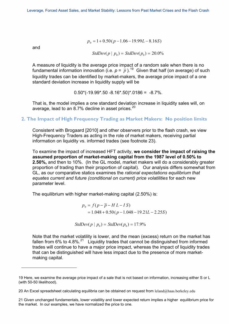
p0 1 0.50( p 1.06 19.99L 8.16S)

StdDev( p | p0 ) StdDev( p0 ) 20.0% and

A measure of liquidity is the average price impact of a random sale when there is no fundamental information innovation (i.e. p = p ).19 Given that half (on average) of such liquidity trades can be identified by market-makers, the average price impact of a one standard deviation increase in liquidity supply will be 0.50*(-19.99*.50 -8.16*.50)*.0186 = -8.7%. That is, the model implies a one standard deviation increase in liquidity sales will, on average, lead to an 8.7% decline in asset prices.20

2. The Impact of High Frequency Trading as Market Makers: No position limits

Consistent with Brogaard [2010] and other observers prior to the flash crash, we view High-Frequency Traders as acting in the role of market makers, receiving partial information on liquidity vs. informed trades (see footnote 23). To examine the impact of increased HFT activity, we consider the impact of raising the assumed proportion of market-making capital from the 1987 level of 0.50% to 2.50%, and then to 10%. (In the GL model, market makers will do a considerably greater proportion of trading than their proportion of capital). Our analysis differs somewhat from GL, as our comparative statics examines the rational expectations equilibrium that equates current and future (conditional on current) price volatilities for each new parameter level. The equilibrium with higher market-making capital (2.50%) is:

)25.221.19048.1(50.0048.1

)(0

SLp

SILHppfp

%9.17)()|( 00 pStdDevppStdDev

Note that the market volatility is lower, and the mean (excess) return on the market has fallen from 6% to 4.8%.21 Liquidity trades that cannot be distinguished from informed trades will continue to have a major price impact, whereas the impact of liquidity trades that can be distinguished will have less impact due to the presence of more market-making capital.

19 Here, we examine the average price impact of a sale that is not based on information, increasing either S or L (with 50-50 likelihood). 20 An Excel spreadsheet calculating equilibria can be obtained on request from [email protected] 21 Given unchanged fundamentals, lower volatility and lower expected return implies a higher equilibrium price for the market. In our examples, we have normalized the price to one.

mailto:[email protected]


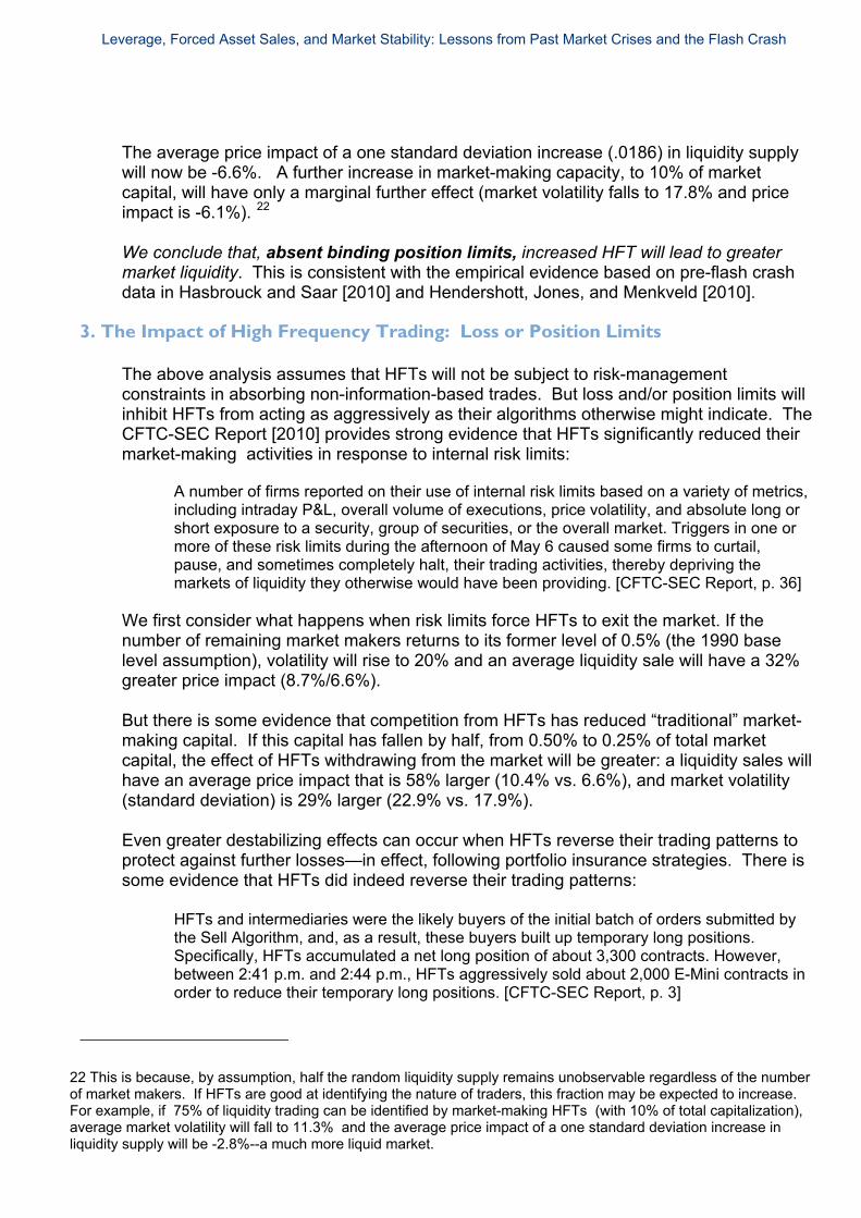
The average price impact of a one standard deviation increase (.0186) in liquidity supply will now be -6.6%. A further increase in market-making capacity, to 10% of market capital, will have only a marginal further effect (market volatility falls to 17.8% and price impact is -6.1%). 22 We conclude that, absent binding position limits, increased HFT will lead to greater market liquidity. This is consistent with the empirical evidence based on pre-flash crash data in Hasbrouck and Saar [2010] and Hendershott, Jones, and Menkveld [2010].

3. The Impact of High Frequency Trading: Loss or Position Limits The above analysis assumes that HFTs will not be subject to risk-management constraints in absorbing non-information-based trades. But loss and/or position limits will inhibit HFTs from acting as aggressively as their algorithms otherwise might indicate. The CFTC-SEC Report [2010] provides strong evidence that HFTs significantly reduced their market-making activities in response to internal risk limits:

A number of firms reported on their use of internal risk limits based on a variety of metrics, including intraday P&L, overall volume of executions, price volatility, and absolute long or short exposure to a security, group of securities, or the overall market. Triggers in one or more of these risk limits during the afternoon of May 6 caused some firms to curtail, pause, and sometimes completely halt, their trading activities, thereby depriving the markets of liquidity they otherwise would have been providing. [CFTC-SEC Report, p. 36]

We first consider what happens when risk limits force HFTs to exit the market. If the number of remaining market makers returns to its former level of 0.5% (the 1990 base level assumption), volatility will rise to 20% and an average liquidity sale will have a 32% greater price impact (8.7%/6.6%). But there is some evidence that competition from HFTs has reduced “traditional” market-making capital. If this capital has fallen by half, from 0.50% to 0.25% of total market capital, the effect of HFTs withdrawing from the market will be greater: a liquidity sales will have an average price impact that is 58% larger (10.4% vs. 6.6%), and market volatility (standard deviation) is 29% larger (22.9% vs. 17.9%). Even greater destabilizing effects can occur when HFTs reverse their trading patterns to protect against further losses—in effect, following portfolio insurance strategies. There is some evidence that HFTs did indeed reverse their trading patterns:

HFTs and intermediaries were the likely buyers of the initial batch of orders submitted by the Sell Algorithm, and, as a result, these buyers built up temporary long positions. Specifically, HFTs accumulated a net long position of about 3,300 contracts. However, between 2:41 p.m. and 2:44 p.m., HFTs aggressively sold about 2,000 E-Mini contracts in order to reduce their temporary long positions. [CFTC-SEC Report, p. 3]

22 This is because, by assumption, half the random liquidity supply remains unobservable regardless of the number of market makers. If HFTs are good at identifying the nature of traders, this fraction may be expected to increase. For example, if 75% of liquidity trading can be identified by market-making HFTs (with 10% of total capitalization), average market volatility will fall to 11.3% and the average price impact of a one standard deviation increase in liquidity supply will be -2.8%--a much more liquid market.


A key question is whether other market participants can predict (or observe) the forced selling (p0) that results from risk management. GL consider three cases:

1. (p0) is observed by no investors 2. (p0) is observed only supply-informed investors (“market makers”) 3. (p0) is observed by all investors

In their base case, GL (p. 1010) show that if 5% of investors follow a totally unobserved put replicating strategy, with losses limited to 10%, the resulting selling can result in a positive-feedback “crash” of 35%, when fundamentals deteriorate less than 2%. Markets are much more stable if forced selling can be observed by market makers, and highly stable if all investors know the extent of forced selling induced by portfolio insurance.

leverage, forced asset sales, and market stability ... · historical examples of forced selling and...

Documents