lessons learned with performance prediction and design patterns on molecular dynamics brian holland...

Lessons Learned with Lessons Learned with Performance Prediction and Performance Prediction and Design Patterns on Design Patterns on Molecular DynamicsMolecular Dynamics

Brian HollandKarthik Nagarajan

Saumil MerchantHerman Lam

Alan D. George

2

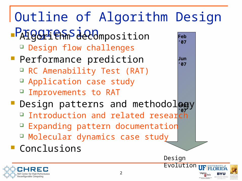
Outline of Algorithm Design Progression Algorithm decomposition

Design flow challenges Performance prediction

RC Amenability Test (RAT) Application case study Improvements to RAT

Design patterns and methodology Introduction and related research Expanding pattern documentation Molecular dynamics case study

Conclusions

Feb ‘07

Jun ‘07

Sept ‘07

Design Evolution

3

Design Flow Challenges Original mission

Create scientific applications for FPGAs as case studies to investigate topics such as portability and scalability Molecular dynamics is one such application

Maximize performance and productivity using HLLs and high-performance reconfigurable computing (HPRC) Applications should have significant speedup over SW baseline

Challenges Ensuring speedup over traditional implementations

Particularly when researcher is not RC oriented Exploring design space efficiently

Several designs may achieve speedup but which should be used?

4

Algorithm Performance Premises

(Re)designing applications is expensive Only want to design once and even then, do it efficiently

Scientific applications can contain extra precision Floating point may not be necessary but is a SW “standard”

Optimal design may overuse available FPGA resources Discovering resource exhaustion mid-development is expensive

Need Performance prediction

Quickly and with reasonable accuracy estimate the performance of a particular algorithm on a specific FPGA platform

Utilize simple analytic models to make prediction accessible to novices

5

Introduction RC Amenability Test

Methodology for rapidly analyzing a particular algorithm’s design compatibility to a specific FPGA platform and projecting speedup

Importance of RAT Design migration process is lengthy and costly

Allows for detailed consideration with potential tradeoff analyses Creates formal procedure reducing need for “expert” knowledge

Scope of RAT RAT cannot make generalizations about applications

Different algorithm choices will greatly affect application performance Different FPGA platform architectures will affect algorithm capabilities

6

RAT Methodology Throughput Test

Algorithm and FPGA platform are parameterized

Equations are used to predict speedup

Numerical Precision Test RAT user should explicitly

examine the impact of reducing precision on computation

Interrelated with throughput test Two tests essentially proceed

simultaneously Resource Utilization Test

FPGA resources usage is estimated to determine scalability on FPGA platform

Overview of RAT Methodology

7

Related Work Performance prediction via parameterization

“The performance analysis in this paper is not real performance prediction; rather it targets the general concern of whether or not an algorithm will fit within the memory subsystem that is designed to feed it.“ [1] (Illinois) Applications decomposed to determine total size and computational density Computational platforms characterized by memory size, bandwidth, and latency

Parallel, heterogeneous shared RC resource modeling [2] (ORNL) System-level modeling for multi-FPGA augmented systems

Other performance prediction research Performance Prediction Model (PPM) [3] Optimizing hardware function evaluation [4]

Comparable models for conventional parallel processing systems Parallel Random Access Machine (PRAM) [5] LogP [6]

8

Throughput Methodology

Parameterize key components of algorithm to estimate runtime

Use equations to determine execution time of RC application

Compare runtime with SW baseline to determine projected speedup

Explore ranges of values to examine algorithm performance bounds

Terminology Element

Basic unit of data for the algorithm that determines the amount of computation

e.g. Each character (element) in a string matching algorithm will require some number of computations to complete

Operation Basic unit of work which helps

complete a data element e.g. Granularity can vary greatly

depending upon formulation. 1 Multiply or 16 shifts could represent 1

or 16 operations, respectively

Nelements, input (elements)

Nelements, output (elements)

Nbytes/element (bytes/element)

throughput(ideal) (Mbps)

α(input) 0<α<1

α(output) 0<α<1

Nops/element (ops/element)

throughput(proc) (ops/cycle)

f(clock) (MHz)

t(soft) (sec)

N (iterations)

Dataset Parameters

Communication Parameters

Computation Parameters

Software Parameters

RAT Input Parameters

9

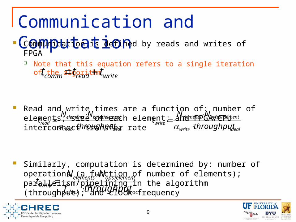
Communication and Computation Communication is defined by reads and writes of FPGA

Note that this equation refers to a single iteration of the algorithm

Read and write times are a function of: number of elements; size of each element; and FPGA/CPU interconnect transfer rate

Similarly, computation is determined by: number of operations (a function of number of elements); parallelism/pipelining in the algorithm (throughput); and clock frequency

writereadcomm ttt

idealread

elementbyteselementsread throughput

NNt

/

procclock

elementopselementscomp throughputf

NNt

/

idealwrite

elementbyteselementswrite throughput

NNt

/

10

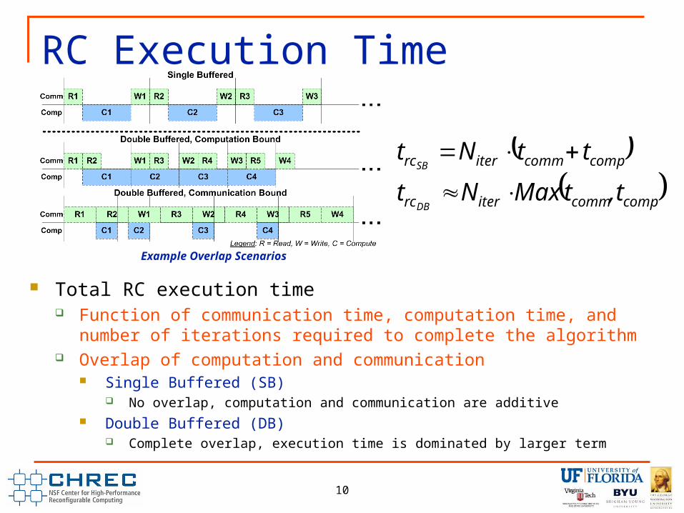
RC Execution Time

Total RC execution time Function of communication time, computation time, and number of

iterations required to complete the algorithm Overlap of computation and communication

Single Buffered (SB) No overlap, computation and communication are additive

Double Buffered (DB) Complete overlap, execution time is dominated by larger term

compcommiterrc

compcommiterrc

t,tMaxNt

ttNt

DB

SB

Example Overlap Scenarios

11

Performance Equations Speedup

Compares predicted performance versus software baseline Shows performance as a function of total execution time

Utilization Computation utilization shows effective idle time of FPGA Communication utilization illustrates interconnect saturation

RC

soft

t

tspeedup

compcomm

commcomm

compcomm

compcomp

ttMax

tutil

ttMax

tutil

DB

DB

,

,

compcomm

commcomm

compcomm

compcomp

tt

tutil

tt

tutil

SB

SB

12

Numerical Precision Applications should have minimum level of precision

necessary to remain within user tolerances SW applications will often have extra precision due to coarse-grain

data types of general-purpose processors Extra precision can be wasteful in terms of performance and

resource utilization on FPGAs

Automated fixed-point to floating-point conversion Useful for exploring reduced precision in algorithm designs Often requires additional coding to explore options

Ultimately, user must make final determination on precision RAT exists to help explore computation performance aspects of

application, just as it helps investigate other algorithmic tradeoffs

13

Resource Utilizations Intended to prevent designs that cannot be

physically realized in FPGAs On-Chip RAM

Includes memory for application core and off-chip I/O Relatively simple to examine and scale prior to hardware design

Hardware Multipliers Includes variety of vendor-specific multipliers and/or MAC units Simple to compute usage with sufficient device knowledge

Logic Elements Includes look-up tables and other basic registering logic Extremely difficult to predict usage before hardware design

14

Probability Density Function Estimation Parzen window probability

density function (PDF) estimation Computation complexity

O(Nnd) N – number of discrete

probability levels (i.e. bins) n – number of discrete points

where probability is estimated d – number of dimensions

Intended architecture Eight parallel kernels each

compute the discrete points versus a subset of the bins

Incoming data samples are processed against 256 bins

Chosen 1-D PDF algorithm architecture

15

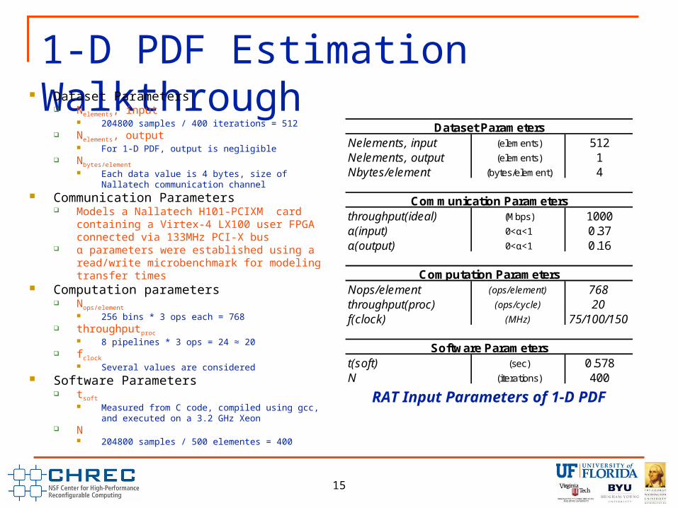
1-D PDF Estimation Walkthrough Dataset Parameters

Nelements, input 204800 samples / 400 iterations = 512

Nelements, output For 1-D PDF, output is negligible

Nbytes/element Each data value is 4 bytes, size of Nallatech

communication channel Communication Parameters

Models a Nallatech H101-PCIXM card containing a Virtex-4 LX100 user FPGA connected via 133MHz PCI-X bus

α parameters were established using a read/write microbenchmark for modeling transfer times

Computation parameters Nops/element

256 bins * 3 ops each = 768 throughputproc

8 pipelines * 3 ops = 24 ≈ 20 fclock

Several values are considered Software Parameters

tsoft Measured from C code, compiled using gcc, and

executed on a 3.2 GHz Xeon N

204800 samples / 500 elementes = 400

Nelements, input (elements) 512Nelements, output (elements) 1Nbytes/element (bytes/element) 4

throughput(ideal) (Mbps) 1000α(input) 0<α<1 0.37α(output) 0<α<1 0.16

Nops/element (ops/element) 768throughput(proc) (ops/cycle) 20f(clock) (MHz) 75/100/150

t(soft) (sec) 0.578N (iterations) 400

Dataset Parameters



Software Parameters

RAT Input Parameters of 1-D PDF

16

1-D PDF Estimation Walkthrough Frequency

Difficult to predict a priori Several possible values are explored

Prediction accuracy Communication accuracy was low

Despite microbenchmarking, communication was longer than expected

Minor inaccuracies in timing for small transfers compounded over 400 iterations for 1-D PDF

Computational accuracy was high Throughput was rounded from 24

ops/cycle to 20 ops/cycle Conservative parallelism was

warranted due to unaccounted pipeline stalls

Algorithm constructed in VHDL

Predicted Predicted Predicted Actual

f(clock) 75 100 150 150tcomm 5.56E-6 5.56E-6 5.56E-6 2.50E-5tcomp 2.62E-4 1.97E-4 1.31E-4 1.39E-4utilcomm 2% 3% 4% 15%utilcomp 98% 97% 96% 85%tRC 1.07E-1 8.09E-2 5.46E-2 7.45E-2speedup 5.4 7.2 10.6 7.8

FPGA Resource Utilization48-bit DSPs 8%

BRAMs 15%

Slices 16%

secE.

secE.secE.iterationst

secE.

secops

E

ops

cycleops

MHz

elementops

elementst

SBRC

comp

2465

43116565400

431193

393216

20150

768512

Performance Parameters of 1-D PDF

Example Computations from RAT Analysis

17

2-D PDF Estimation Dimensionality

PDF can extend to multiple dimensions

Significantly increases computational complexity and volume of communication

Algorithm Same construction as 1-D PDF

Written in VHDL Targets Nallatech H101

Xilinx V4LX100 FPGA PCI-X interconnect

Prediction Accuracy Communication

Similar to 1-D PDF, communication times were underestimated

Computation Computation was smaller than

expected, balancing overall execution time





Dataset Parameters



Software Parameters

FPGA Resource Utilization48-bit DSPs 33%

BRAMs 21%

Slices 22%

Performance Parameters of 2-D PDF

RAT Input Parameters of 2-D PDF

Predicted Predicted Predicted Actualf(clock) 75 100 150 150tcomm 1.65E-3 1.65E-3 1.65E-3 1.06E-2tcomp 1.12E-1 8.39E-2 5.59E-2 4.46E-2utilcomm 1% 2% 3% 19%utilcomp 99% 98% 97% 81%tRC 4.54E+1 3.42E+1 2.30E+1 2.21E+1speedup 3.5 4.6 6.9 7.2

18

Molecular Dynamics Simulation of physical interaction

of a set of molecules over a given time interval Based upon code provided by Oak

Ridge National Lab (ORNL) Algorithm

16,384 molecule data set Written in Impulse C XtremeData XD1000 platform

Altera Stratix-II EPS2180 FPGA HyperTransport interconnect

SW baseline on 2.4GHz Opteron Challenges for accurate prediction

Nondeterministic runtime Molecules beyond a certain

threshold are assumed to have zero impact

Large datasets for MD Exhausts FPGA local memory





Dataset Parameters



Software Parameters


f(clock) 75 100 150 100tcomm 2.62E-3 2.62E-3 2.62E-3 1.39E-3tcomp 7.17E-1 5.37E-1 3.58E-1 8.79E-1utilcomm 0.4% 0.5% 0.7% 0.2%utilcomp 99.6% 99.5% 99.3% 99.8%tRC 7.19E-1 5.40E-1 3.61E-1 8.80E-1speedup 8 10.7 16 6.6

FPGA Resource Utilization

48-bit DSPs 100%

BRAMs 24%

Slices 73%

RAT Input Parameters of MD

Performance Parameters of MD

19

Conclusions RC Amenability Test

Provides simple, fast, and effective method for investigating performance potential of given application design for a given target FPGA platform

Works with empirical knowledge of RC devices to create more efficient and effective means for application design

When RAT-projected speedups are found to be disappointing, designer can quickly reevaluate their algorithm design and/or RC platform selected as target

Successes Allows for rapid algorithm analysis before any significant hardware coding Demonstrates reasonably accurate predictions despite coarse parameterization

Applications Showcases effectiveness of RAT for deterministic algorithms like PDF estimation Provides valuable qualitative insight for nondeterministic algorithms such as MD

Future Work Improve support for nondeterministic algorithms through pipelining Explore performance prediction with applications for multi-FPGA systems Expand methodology for numerical precision and resource utilization

20

Molecular Dynamics Revisited

21

Molecular Dynamics Algorithm

16,384 molecule data set Written in Impulse C XtremeData XD1000 platform

Altera Stratix II EPS2180 FPGA HyperTransport interconnect

SW baseline on 2.4GHz Opteron Parameters

Dataset Parameters Model volume of data used by FPGA

Communication Parameters Model the HyperTransport Interconnect

Computation Parameters Model computational requirement of FPGA Nops/element

164000 ≈ 16384 * 10 ops i.e. each molecule (element) takes 10ops/iteration

Throughputproc 50 i.e. operations per cycle needed for >10x speedup

Software Parameters Software baseline runtime and iterations

required to complete RC application





Dataset Parameters



Software Parameters



RAT Input Parameters of MD


22

Parameter Alterations for Pipelining MD Optimization

Each molecular computation should be pipelined

Focus becomes less on individual molecules and more on molecular interactions

Parameters Computation Parameters

Nops/element 16400 Strictly number of interactions per

element Throughputpipeline

.333 Number of cycles needed to per

interaction. i.e. you can only stall pipeline for 2 extra cycles

Npipeline 15 Guess based on predicted area

usage



Nops/element (ops/element) 16400throughput(pipeline) (ops/cycle) 0.33333Npipelines (ops/cycle) 15f(clock) (MHz) 75/100/150


Dataset Parameters



Software Parameters

Modified RAT Input Parameters of MD




23

Pipelined Performance Prediction Molecular Dynamics

If a pipeline is possible, certain parameters become obsolete The number of operations in the

pipeline (i.e depth) is not important The number of pipeline stalls

becomes critical and is much more meaningful for non-deterministic apps

Parameters Nelement

163842

Number of molecular pairs Nclks/element

3 i.e. up to two cycles can be stalls

Npipelines

15 Same number of kernels as before

Nelements (elements) (16384)2

Nclks/element (cycle/element) 3Npipelines 15Depthpipeline cycles 100f(clock) (MHz) 100t(soft) (sec) 5.76

tRC (sec) 0.537Speedup 10.7

Dataset Parameters

Dataset Parameters

commclk

pipeline

clknelsker

element/clkselementsRC t

f

Depth

fN

NNt

Pipelined RAT Input Parameters of MD

24

“And now for something completely different…”

-Monty Python

(Or is it?)

25

Leveraging Algorithm Designs Introduction

Molecular dynamics provided several lessons learned Best design practices for coding in Impulse C Algorithm optimizations for maximum performance Memory staging for minimal footprint and delay

Sacrificing computation efficiency for decreased memory accesses

Motivations and Challenges Application design should educate the researcher

Designs should also trainer other researchers Unfortunately, new designing can be expensive

Collecting application knowledge into design patterns provides distilled lessons learned for efficient application

2626

Design Patterns Objected-oriented software engineering:

“A design pattern names, abstracts, and identifies the key aspects of a common design structure that make it useful for creating a reusable object-oriented design” (1)

Reconfigurable Computing “Design patterns offer us organizing and

structuring principles that help us understand how to put building blocks (e.g., adders, multipliers, FIRs) together.” (2)

(1) Gamma, Eric, et.al., Design Patterns: Elements of Reusable Object-Oriented Software, Addison-Wesley, Boston, 1995.

(2) DeHon, Andre, et. Al., “Design Patterns for Reconfigurable Computing”, Proceedings of 12th IEEE Symposium on Field-Programmable Custom Computing Machines (FCCM’04), April 20-23, 2004, Napa, California.

27

Classificaiton of Design Patterns – OO Text Book(1) Pattern categories

Creational Abstract Factory Prototype Singleton Etc.

Structural Adapter Bridge Proxy Etc.

Behavioral Iterator Mediator Interpreter Etc.

27

Describing Patterns Pattern name Intent Also know as Motivation Applicability Structure Participants Collaborations Consequences Implementation Sample code Known uses Related patterns

2828

Sample Design Patterns – RC Paper (2) 14 pattern categories: Area-Time Tradeoffs Expressing Parallelism Implementing Parallelism Processor-FPGA Integration Common-Case Optimization Re-using Hardware Efficiently Specialization Partial Reconfiguration Communications Synchronization Efficient Layout and Communications Implementing Communication Value-Added Memory Patterns Number Representation Patterns

89 patterns identified (samples) Course-Grained Time Multiplexing Synchronous Dataflow Multi-threaded Sequential vs. Parallel Design

(hardware-software partitioning) SIMD Communicating FSMDs Instruction augmentation Exceptions Pipelining Worst-Case Footprint Streaming Data Shared Memory Synchronous Clocking Asynchronous Handshaking Cellular Automata Etc

29

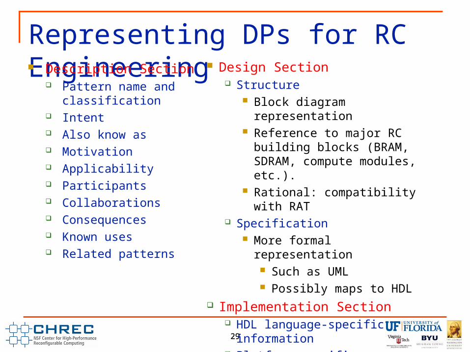
Representing DPs for RC Engineering

29

Description Section Pattern name and

classification Intent Also know as Motivation Applicability Participants Collaborations Consequences Known uses Related patterns

Design Section Structure

Block diagram representation Reference to major RC building

blocks (BRAM, SDRAM, compute modules, etc.).

Rational: compatibility with RAT Specification

More formal representation Such as UML Possibly maps to HDL

Implementation Section HDL language-specific information Platform specific information Sample code

3030

Example – Time Multiplexing Pattern

Intent – Large designs on small or fixed capacity platforms

Motivation – Meet real-time needs or inadequate design space

Applicability – For slow reconfiguration• No feedback loops (acyclic dataflow)

Participants – Subgraphs

*DeH

on e

t al,

2004

* Computational graph divided into smaller subgraphs

Collaborations – Control algorithm directs subgraphs swapping Consequences – Slow reconfiguration time, large buffers & imperfect

device resource utilization Known Uses – Video processing, target recognition Implementation – Conventional processor issues commands for

reconfiguration and collaboration

3131

Example – Datapath Duplication

Intent – Exploiting computation parallelism in sequential programming structures (loops)

Motivation – Achieving faster performance through replication of computational structures

Applicability – data independent• No feedback loops (acyclic dataflow)

Participants – Single computational kernel

* Replicated computational structures for parallel processing

Collaborations – Control algorithm directs dataflow and synchronization Consequences – Area time tradeoff, higher processing speed at the cost

of increased implementation footprint in hardware Known Uses – PDF estimation, BbNN implementation, MD, etc. Implementation – Centralize controller orchestrates data movement and

synchronization of parallel processing elements

32

System-level patterns for MD

When design MD, initial goal is decompose algorithm into parallel kernels “Datapath duplication” is a

potential starting pattern MD will require additional

modifications since computational structure will not divide cleanly

Visualization of Datapath Duplication

“What do customers buy after viewing this item?”

67% use this pattern37% alternatively use ….

“May we also recommend?”PipeliningLoop Fusion

“On-line Shopping” for Design Patterns

33

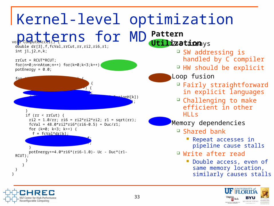
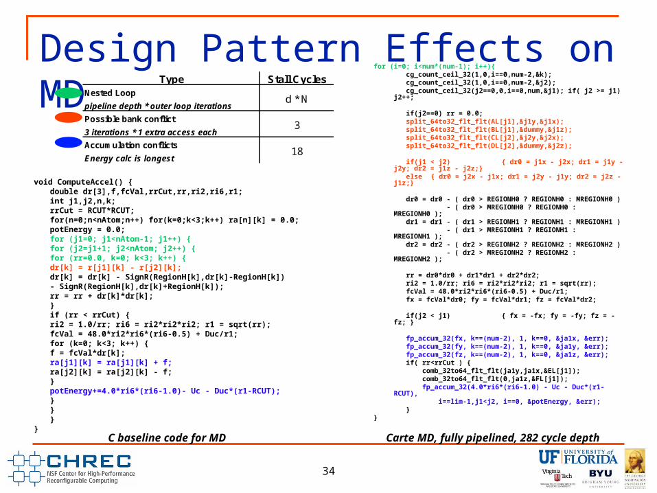
void ComputeAccel() {double dr[3],f,fcVal,rrCut,rr,ri2,ri6,r1;int j1,j2,n,k;

rrCut = RCUT*RCUT;for(n=0;n<nAtom;n++) for(k=0;k<3;k++) ra[n][k] = 0.0;potEnergy = 0.0;

for (j1=0; j1<nAtom-1; j1++) {for (j2=j1+1; j2<nAtom; j2++) {for (rr=0.0, k=0; k<3; k++) {dr[k] = r[j1][k] - r[j2][k];dr[k] = dr[k]-SignR(RegionH[k],dr[k]-RegionH[k])

- SignR(RegionH[k],dr[k]+RegionH[k]);rr = rr + dr[k]*dr[k];

}if (rr < rrCut) {ri2 = 1.0/rr; ri6 = ri2*ri2*ri2; r1 = sqrt(rr);fcVal = 48.0*ri2*ri6*(ri6-0.5) + Duc/r1;for (k=0; k<3; k++) {f = fcVal*dr[k];ra[j1][k] = ra[j1][k] + f;ra[j2][k] = ra[j2][k] - f;

}potEnergy+=4.0*ri6*(ri6-1.0)- Uc - Duc*(r1-

RCUT);}

} }

}

Kernel-level optimization patterns for MD

2-D arrays SW addressing is handled

by C compiler HW should be explicit

Loop fusion Fairly straightforward in

explicit languages Challenging to make

efficient in other HLLsMemory dependencies

Shared bank Repeat accesses in pipeline

cause stalls Write after read

Double access, even of same memory location, similarly causes stalls

Pattern Utilization

34

Design Pattern Effects on MD

for (i=0; i<num*(num-1); i++){ cg_count_ceil_32(1,0,i==0,num-2,&k); cg_count_ceil_32(1,0,i==0,num-2,&j2); cg_count_ceil_32(j2==0,0,i==0,num,&j1); if( j2 >= j1) j2++;

if(j2==0) rr = 0.0; split_64to32_flt_flt(AL[j1],&j1y,&j1x); split_64to32_flt_flt(BL[j1],&dummy,&j1z); split_64to32_flt_flt(CL[j2],&j2y,&j2x); split_64to32_flt_flt(DL[j2],&dummy,&j2z);

if(j1 < j2) { dr0 = j1x - j2x; dr1 = j1y - j2y; dr2 = j1z - j2z;} else { dr0 = j2x - j1x; dr1 = j2y - j1y; dr2 = j2z - j1z;}

dr0 = dr0 - ( dr0 > REGIONH0 ? REGIONH0 : MREGIONH0 ) - ( dr0 > MREGIONH0 ? REGIONH0 : MREGIONH0 ); dr1 = dr1 - ( dr1 > REGIONH1 ? REGIONH1 : MREGIONH1 ) - ( dr1 > MREGIONH1 ? REGIONH1 : MREGIONH1 ); dr2 = dr2 - ( dr2 > REGIONH2 ? REGIONH2 : MREGIONH2 ) - ( dr2 > MREGIONH2 ? REGIONH2 : MREGIONH2 );

rr = dr0*dr0 + dr1*dr1 + dr2*dr2; ri2 = 1.0/rr; ri6 = ri2*ri2*ri2; r1 = sqrt(rr); fcVal = 48.0*ri2*ri6*(ri6-0.5) + Duc/r1; fx = fcVal*dr0; fy = fcVal*dr1; fz = fcVal*dr2;

if(j2 < j1) { fx = -fx; fy = -fy; fz = -fz; }

fp_accum_32(fx, k==(num-2), 1, k==0, &ja1x, &err); fp_accum_32(fy, k==(num-2), 1, k==0, &ja1y, &err); fp_accum_32(fz, k==(num-2), 1, k==0, &ja1z, &err); if( rr<rrCut ) { comb_32to64_flt_flt(ja1y,ja1x,&EL[j1]); comb_32to64_flt_flt(0,ja1z,&FL[j1]); fp_accum_32(4.0*ri6*(ri6-1.0) - Uc - Duc*(r1-RCUT), i==lim-1,j1<j2, i==0, &potEnergy, &err); }}

void ComputeAccel() {double dr[3],f,fcVal,rrCut,rr,ri2,ri6,r1;int j1,j2,n,k;rrCut = RCUT*RCUT;for(n=0;n<nAtom;n++) for(k=0;k<3;k++) ra[n][k] = 0.0;potEnergy = 0.0;for (j1=0; j1<nAtom-1; j1++) {

for (j2=j1+1; j2<nAtom; j2++) {for (rr=0.0, k=0; k<3; k++) {

dr[k] = r[j1][k] - r[j2][k];dr[k] = dr[k] - SignR(RegionH[k],dr[k]-RegionH[k])

- SignR(RegionH[k],dr[k]+RegionH[k]);rr = rr + dr[k]*dr[k];

}if (rr < rrCut) {

ri2 = 1.0/rr; ri6 = ri2*ri2*ri2; r1 = sqrt(rr);fcVal = 48.0*ri2*ri6*(ri6-0.5) + Duc/r1;for (k=0; k<3; k++) {

f = fcVal*dr[k];ra[j1][k] = ra[j1][k] + f;ra[j2][k] = ra[j2][k] - f;

}potEnergy+=4.0*ri6*(ri6-1.0)- Uc - Duc*(r1-RCUT);

} }

}} Carte MD, fully pipelined, 282 cycle

depth

Type Stall CyclesNested Loop

pipeline depth * outer loop iterations

Possible bank conflict

3 iterations * 1 extra access each

Accumulation conflicts

Energy calc is longest

d * N

3

18

C baseline code for MD

35

Conclusions

Performance prediction is a powerful technique for improving efficiency of RC application formulation Provides reasonable accuracy for the rough estimate Encourages importance of numerical precision and resource

utilization in performance prediction

Design patterns provide lessons learned documentation Records and disseminates algorithm design knowledge Allows for more effective formulation of future designs

Future Work Improve connection b/w design patterns and performance prediction Expand design pattern methodology for better integration with RC Increase role of numerical precision in performance prediction

lessons learned with performance prediction and design patterns on molecular dynamics brian holland...

Documents