Lesson 26: Taylor series and asymptotic seriesrestart;

One that convergesI don't think there's an easy way in general to tell whether a series solution to a functional equation will have a positive radius of convergence. Here's one where the radius does turn out to be positive.

eq := A(x) = A(2*x)^2/4 + x;

Again, when , so a series about might work. For we haveeval(eq,x=0);

solve(%,A(0));

I'll try for .Aseries:= unapply(4 + add(a[j]*x^j,j=1..20),x);

eval(eq,A=Aseries);

eqs:= {seq(coeff(lhs(%)-rhs(%),x,j),j=1..20)}:

solve(%);

As:= unapply(eval(Aseries(x),%),x);

Aapprox:= evalf(As(x));

What's the radius of convergence?with(plots):

pointplot([seq([j,abs(coeff(Aapprox,x,j))^(1/j)], j=1..20)]);

2 4 6 8 10 12 14 16 18 20

pointplot([seq([j, ln(abs(coeff(Aapprox,x,j)))], j=1..20)]);

(1.2)(1.2)

(1.1)(1.1)

2 4 6 8 10 12 14 16 18 20

It looks very much like these are approaching a straight line. The slope should be approximatelyslope:= ln(abs(coeff(Aapprox,x,20)))-ln(abs(coeff(Aapprox,x,

19)));

So the radius of convergence should be approximatelyexp(-slope);

6.196527162This is probably not very accurate, though.

Integration using seriesHere's another use of Taylor series.

What is the arc length of the ellipse ?

y1 := b*sqrt(1-x^2);

g := sqrt(1+diff(y1,x)^2);

L := 4*Int(g,x=0..1);

EE:=value(L);

This integral is actually the definition of the special function EllipticE, so in itself that's not saying much.

FunctionAdvisor(definition,EllipticE(p));

plot(EE,b=0..5);

b0 1 2 3 4 5

4

6

8

10

12

14

16

18

20

We might try writing the integrand as a series in powers of b. I'll stick that 4 inside the integral.S:= taylor(4*g,b,10);

That won't work: the integrals of each term over will diverge.How about in powers of ? Note that makes our ellipse into a circle.

S:= taylor(4*g,b=1,10);

At first sight this looks just as bad, but it really isn't: the square root gives us an improper integral that converges. Now we'll want to integrate each term for . A convenient way of doing something to every term of a series is with the map command.

map(int,%,x=0..1);

What map does is take a function or command and a Maple object and produce a new object with the function applied to each operand of the object. Thus for a list:

map(t -> t^2, [a,b,c]);

Or for a sum of terms:map(sin,a+b+c);

If there are extra arguments, they are included in each function call. For example:map(F, [a,b,c], d,e);

In our example, the operands of the series structure were the coefficients of the series, and so for each term Maple integrated the coefficient on and made that the corresponding coefficient of the new series.Of course it's quicker to just use the taylor command.

LE:= taylor(EE,b=1,40);

By the way, does it have a Maclaurin series?taylor(EE,b=0,20);

Error, does not have a taylor expansion, try series()

(2.2)(2.2)

(2.1)(2.1)

series(EE,b=0,10);

What's the radius of convergence of the series around b=1?pointplot([seq([n, ln(abs(coeff(LE,b-1,n)))],n=1..39)]);

P:= %:

5 10 15 20 25 30 350

This doesn't look very much like a straight line. Actually it's approximately a constant plus a linear term plus a logarithmic term. There is a command Fit in the Statistics package that can be used to fit a curve to data.

Data:= evalf([seq(ln(abs(coeff(LE,b-1,n))),n=3..39)]);

(2.4)(2.4)

(2.2)(2.2)

(2.1)(2.1)

(2.5)(2.5)

(2.3)(2.3)Statistics[Fit](a*ln(x)+b+c*x,[$3..39],Data,x);

display([plot(%,x=1..39),P]);

x5 10 15 20 25 30 35

0

2

If this is right, the limiting slope would be mlimit:= limit(diff(%%,x),x=infinity);

and the radius of convergence would be exp(mlimit);

0.9942231662Actually I think R is exactly 1. I'm quite sure it is at most 1, because EllipticE is not twice differentiable at 0.

plot(diff(EE, b),b=-2..2);

(2.2)(2.2)

(2.1)(2.1)

b0 1 2

1

2

3

plot(diff(EE,b$2),b=-2..2);

(2.2)(2.2)

(2.1)(2.1)

(3.1)(3.1)

(2.6)(2.6)

b0 1 2

5

10

15

20

25

30

35

limit(diff(EE,b$2),b=0);

Cutoff for Midterm 2 is here!

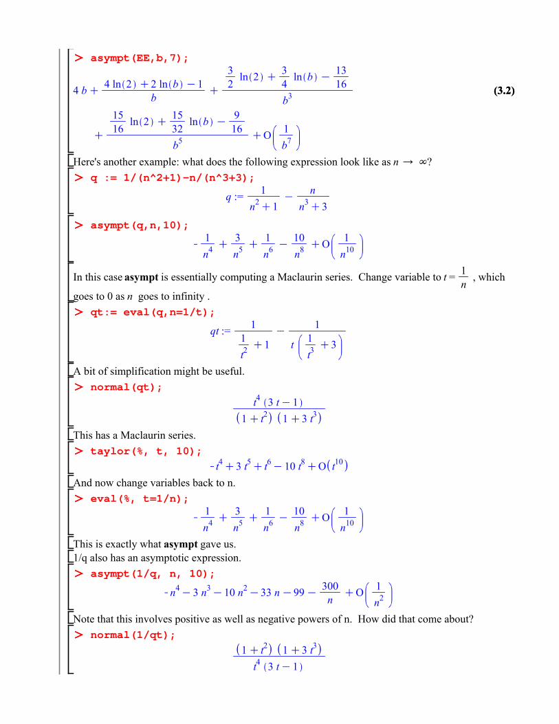
Asymptotic seriesAnother type of series tells us about the behaviour of a function as a variable goes to infinity. Theasympt command will do this. In our example, what happens to the length of the ellipse as ?

asympt(EE,b);

This isn't to be taken quite literally: there's probably a term in there. If we ask for

more terms:

(3.2)(3.2)

(2.2)(2.2)

(2.1)(2.1)

asympt(EE,b,7);

Here's another example: what does the following expression look like as ?q := 1/(n^2+1)-n/(n^3+3);

asympt(q,n,10);

In this case asympt is essentially computing a Maclaurin series. Change variable to , which

goes to 0 as n goes to infinity .qt:= eval(q,n=1/t);

A bit of simplification might be useful.normal(qt);

This has a Maclaurin series.taylor(%, t, 10);

And now change variables back to n.eval(%, t=1/n);

This is exactly what asympt gave us.1/q also has an asymptotic expression.

asympt(1/q, n, 10);

Note that this involves positive as well as negative powers of n. How did that come about?normal(1/qt);

(3.2)(3.2)

(2.2)(2.2)

(2.1)(2.1)

taylor(%, t, 10);

Error, does not have a taylor expansion, try series()

It doesn't have a Maclaurin series because it has a singularity at t = 0 (look at the in the denominator). What it does have is called a Laurent series (in Math 300). In this case you can just

take the Maclaurin series of , and then divide by .

taylor(t^4/qt, t, 10);

convert(%,polynom)/t^4;

expand(%);

eval(%, t=1/n);

Or we could use series instead of taylor, since series can do Laurent series.series(1/qt,t,10);

But not all asymptotic expressions arise in this way.The name asympt is actually a bit unfortunate, because it confuses two quite different ideas: a seriesat infinity, and an asymptotic series.

Asymptotic series for an exponential integralJ := Int(exp(-t)/t, t=x..infinity); value(J);

asympt(%,x,10);

Let's see if we can reproduce this. It's really telling us about a series for .EJ:= exp(x)*J;

(3.2)(3.2)

(2.2)(2.2)

(2.1)(2.1)

We'll use the IntegrationTools package.with(IntegrationTools):

Start with a change of variables, to make the integral go from 0 to infinity.Change(J,t=x+u,u);

J1:= expand(%);

Now has a series in powers of u.

taylor(1/(x+u),u,10);

Using this in our integral should bother you, since the series only converges for , and we're integrating from 0 to . But it's possible to justify this (in Math 301, you might find this called Watson's lemma).

eval(J1,1/(x+u)=convert(%,polynom));

value(%);

expand(%);

It would be nicer to see this sorted by powers of x. The sort command does that.

sort(%,x);

That's what asympt gave us, with one more term.Do you recognize the numbers in the numerators?

(3.2)(3.2)

(2.2)(2.2)

(2.1)(2.1)

(4.1)(4.1)

What if we use the whole series for , rather than just a partial sum?

eq := 1/(x+u) = convert(1/(x+u),FormalPowerSeries,u);

I want to multiply each term by , and integrate from 0 to . Here's a useful integral:Int(exp(-u)*u^k,u=0..infinity);

value(%) assuming k >= 0;

This is actually one definition of the Gamma function.FunctionAdvisor(definition,GAMMA(k));

You know this better as .convert(%%,factorial);

So our series should be

This matches the result from the partial sum. Do you believe this series?For what x does it converge?

Nevertheless, it is useful. Here's another way to get it, which makes the "asymptotic" character of the series clearer, and gives us control over the remainders. I'll use integration by parts.

JS[0] := J1;

JS[1] := Parts(JS[0],1/(x+u));

Note that for , 0 <

Thus we can say .

(3.2)(3.2)

(2.2)(2.2)

(2.1)(2.1)

JS[2] := Parts(JS[1],1/(x+u)^2);

Similarly, so . And so on.

for count from 3 to 8 do

JS[count]:= Parts(JS[count-1],1/(x+u)^count)

end do;

Let's see how well the partial sums of our asymptotic series do at approximating the original integralJ.

for count from 1 to 20 do

PS[count]:= exp(-x)*add((-1)^k*k!/x^(1+k),k=0..count-1)

end do:

plot([value(J),seq(PS[count],count=1..20)],x=0..5,-5..5);

(2.2)(2.2)

(2.1)(2.1)

(3.2)(3.2)

x1 2 3 4 5

0

2

4

Maple objects introduced in this lessonmapFit (in the Statistics package)asympt