lectures onfunctionaldataanalysis - cfe … · ˜mueller/data/pace.html(matlab) variousrpackages....
TRANSCRIPT

LECTURESON FUNCTIONAL DATA ANALYSIS
Hans-Georg MüllerUC Davis
ERCIM
Oviedo, November 2012

OVERVIEW
• PART I: BASICS: MODELING OF RANDOMTRAJECTORES AND LONGITUDINAL DATA
• Functional Principal Component Analysis• Sparse and Dense Functional Data• Derivatives• Empirical Dynamics
• PART II: FUNCTIONAL REGRESSION MODELS• Functional Linear Models• Diagnostics• Functional Dose-Response Models• Functional Additive Regression• Functional Quadratic Regression• Functional Gradients
• PART III: TIME WARPING AND NONLINEARREPRESENTATIONS
• Lecture on Saturday

INTRODUCTION
What characterizes functional data?
Per subject or experimental unit, one samples one or severalfunctions X (t), t ∈ T
High-dimensional (infinite-dimensional) data with a topologycharacterized by order, neighborhood and smoothness – in contrastto MDA (Multivariate Data Analysis).
Commonly adopted model: Data correspond to independentrealizations of a stochastic process with smooth trajectories

LONGITUDINAL STUDIESAND DYNAMICS
Data: Longitudinal studies, e.g. Baltimore Longitudinal on Aging;e-Bay online auction data
Model: Sample of irregularly measured realizations of an underlyingstochastic process, assumed to be smooth
Goals: Estimating derivatives for irregularly sampled randomtrajectories
Learning the underlying dynamics – empirical differential equation
Methods: Functional principal component analysis; Smoothing anddifferentiation (local least squares); Representations of stochasticprocesses

STOCHASTIC PROCESS PERSPECTIVE
Assume observed data are generated by underlying stochasticprocess X ∈ L2(T ) with finite second moments:
µ(t) = E (X (t)) mean functionG (s, t) = cov {X (s),X (t)} covariance function.
Define auto-covariance operator (AG f )(t) =∫
f (s)G (s, t) ds withorthonormal eigenfunctions φk and ordered eigenvaluesλ1 ≥ λ2 ≥ . . .,
(AGφk)(t) = λk φk(t)

Background Material
• Books• Ramsay, J.O. & Silverman, B.W. (2002) Applied Functional
Data Analysis. Springer• Ferraty, F. & Vieu, P. (2006) Nonparametric Functional Data
Analysis. Springer• Horvath, L. & Kokoszka, P. (2012) Inference for Functional
Data with Applications. Springer
• Software• Ramsay’s fda package (Matlab and R versions)• PACE 2.16:
http://anson.ucdavis.edu/∼mueller/data/pace.html (Matlab)• Various R packages

FUNCTIONAL PRINCIPAL COMPONENTS (FPC)KARHUNEN-LOÈVE REPRESENTATION USING FPCs
X (t) = µ(t) +∞∑
k=1
Akφk(t),
where Ak =∫ T0 {X (t)− µ(t)}φk(t)dt, are uncorrelated r.v. with
EAk = 0, EA2k = λk , the functional principal components.
Some key papers:
• Grenander 1950: Basic ideas (following up on Karhunen 1949)• C.R. Rao 1958: Preliminary version for growth curves• Castro, Lawton & Sylvestre 1987: Modes of Variation inindustrial applications
• Rice & Silverman 1991, Rice & C. Wu 2001: B-splines andsystematic study

• Book: Ramsay & Silverman 2005: Presmoothing (usuallyinefficient)
• Bali, Boente, Tyler & J.L. Wang 2012: Systematic study ofrobust FPCA
Why Functional Principal Components?• Parsimonious description of longitudinal/functional data as itis the unique linear representation which explains the highestfraction of variance in the data with a given number ofcomponents.
• Main attraction is equivalence X ≡ {A1,A2, . . .}so that X can be expressed in terms of mean function µ andthe countable sequence of eigenfunctions and uncorrelatedFPC scores Ak .
• For modeling functional regression: Functions f (X ) have anequivalent function g(A1,A2, . . .) so that
f (X ) ≡ g(A1,A2, . . .)

FUNCTIONAL DATA DESIGNS
• Fully observed functions without noise at arbitrarily dense gridMeasurements Yit = Xi (t) available for all t ∈ T ,i = 1, . . . , n :Often unrealistic but mathematically convenient
• Dense design with noisy measurementsMeasurements Yij = Xi (Tij) + εij , where Tij are recorded on aregular grid, Ti1, . . . ,TiNi , and Ni →∞:Applies to typical functional data
• Sparse design with noisy measurements = Longitudinal dataMeasurements Yij = Xi (Tij) + εij , where Tij are random timesand their number Ni per subject is random and finite.
bidtime[i, ]
bids[i
, ]
−4−2
02
4
bidtime[i, ]
bids[i
, ]
bidtime[i, ]
bids[i
, ]
−4−2
02
4
0 50 100 150
bidtime[i, ]
bids[i
, ]0 50 100 150
t (hours)
log(p
rice)
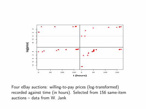
Four eBay auctions: willing-to-pay prices (log-transformed)recorded against time (in hours). Selected from 156 same-itemauctions – data from W. Jank

BALTIMORE LONGITUDINAL STUDYON AGING
• Subset of n = 507 males whose Body Mass Index (BMI) andSystolic Blood Pressure (SBP) were measured at least twicebetween ages 45 and 70 and who survived beyond age 70.
• Measurements are both noisy and spaced irregularly, with boththe measurement times and the number of availablemeasurements varying from subject to subject.

24
26
28
30
32
34
Age (years)
BM
I
Subject 19
Age (years)
Subject 121
Age (years)
Subject 201
Age (years)
Subject 292
45 50 55 60 65
24
26
28
30
32
34
Age (years)
BM
I
Subject 321
45 50 55 60 65Age (years)
Subject 370
45 50 55 60 65Age (years)
Subject 380
45 50 55 60 65 70Age (years)
Subject 391
Observations of BMI for eight randomly selected subjects

100
110
120
130
140
Subject 19
SB
P
Subject 121 Subject 201 Subject 292
45 50 55 60 65
100
110
120
130
140
Subject 321
Age (years)
SB
P
45 50 55 60 65
Subject 370
Age (years)45 50 55 60 65
Subject 380
Age (years)50 60 70
Subject 391
Age (years)
Observations of SBP for eight randomly selected subjects

PACE
Principal Analysis by Conditional Expectation (Yao, M, Wang2005ab, Liu & M 2009) to obtain components of the functionalprincipal component representation for all of these designs.
Idea: Borrowing strength from entire sample for estimation ofindividual trajectories
Implementation steps:
• Mean function: Smoothing across all pooled observations• Covariance surface: Pooling products for pairs of observationsfrom the same subject, then smoothing – denoising is achievedby separating out the diagonal (Staniswalis & Lee 1998)
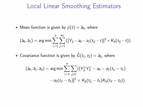
Local Linear Smoothing Estimators
• Mean function is given by µ(t) = a0, where
(a0, a1) = argminn∑
i=1
mi∑j=1
{[Yij−a0−a1(tij−t)]2×Kh(tij−t)}.
• Covariance function is given by G (t1, t2) = a0, where
(a0, a1, a2) = argminn∑
i=1
∑j 6=l
{[Y cij Y
cil − a0 − a1(tij − t1)
−a2(til − t2)]2 × Kb(tij − t1)Kb(til − t2)}.

G(s,t)
G(t,t)+σ2
t s t
Relationship between the covariance surface and variances on thediagonal: Decomposing diagonal into error and covariancecomponents.

IMPLEMENTATION ISSUES
• Obtain eigenvalues/eigenfunctions:
For k-th eigenvalue/eigenfunction pair (λk , φk) use discretizedversions of eigenequations,∫ T
0cov(X (s),X (t))φk(s)ds = λkφk(t),
s.t.∫ T0 φk(t)2dt = 1,
∫ T0 φk(t)φm(t)dt = 0, m 6= k ,
substituting smoothed estimates for the covariance surface.• Project initial smoothed covariance estimates on space ofnon-negative definite covariance matrices: (Hall, M, Yao 2008)
ˆcov(X (s),X (t)) =K∑
k=1,λk>0
λk φk(s)φk(t).

• Obtain Functional principal components (the random effects):• Conditioning E (Ak |Ui ), where Ui is the vector of available
data for the i-th subject (random dimension)• Best linear predictor for conditional expectation (best predictor
under Gaussian assumptions)• Substitute estimates for eigenvalues, eigenfunctions,
covariances• Regularization for inverses of cova matrices at random
locations• Choice of regularization parameters (number of included
components, smoothing parameters: GCV, FVE, BIC,. . .)
• Implementation of FPCA and functional regression models:PACE 2.14 at:http://anson.ucdavis.edu/∼mueller/data/programs.html

ESTIMATING DERIVATIVES FROM SPARSE DATADifferentiating Karhunen-Loève representation:
X (ν)i (t) = µ(ν)(t) +
∞∑k=1
Aikφ(ν)k (t), ν = 0, 1, . . . .
• Obtain estimated random effects Aik by conditioning as before• Estimate µ(ν)(t) by known nonparametric 1-d differentiation,applied to pooled scatterplots.
• How to obtain φ(ν)k ? Observe
dν
dtν
∫T
G (t, s)φk(s)ds = λkdν
dtνφk(t),
implying
φ(ν)k (t) =
1λk
∫T
∂ν
∂tνG (t, s)φk(s)ds.

0 12 24 36 48 60 72 84 96 108 120 132 144 1560
12
24
36
48
60
72
84
96
108
120
132
144
156
�����
����
Locations of all pairs of points where bids are recorded for auctiondata.

Estimated covariance surface from all pairs and estimated partialderivative surface for auction data.

●●
●
●
●●
●●●
●
●
●●●
●
●●
●
●
●
●
●●●
●
●
●
●
●
●
●
●
●
●
●●●
●●
●
●●●
●
●●
●
●
●
●●●●●●
●
●●●
●
●
●
●
●
●●●
●
●●●
●
●●●
●
●●
●●
●
●●
●
●●
●
●
●●●
●
●●
●
●
●
●
●
●
●
●
●
●
●
●●●
●
●
●●
●●●
●
●
●●
●
●●●
●
●
●
●
●●●
●
●
●
●
●●●
●●
●
●●
●
●
●
●
●●
●
●●●●
●
●
●
●●
●
●
●●
●●●
●
●
●● ●
●
● ●
●
●
●
●
●● ●
●
●
●
●
●
●
●
●
●
●
●● ●
●●
●
● ●●
●
●●
●
●
●
●●●●●●
●
●● ●
●
●
●
●
●
●●●
●
●●●
●
●● ●
●
● ●
●●
●
●●
●
● ●
●
●
●●●
●
●●
●
●
●
●
●
●
●
●
●
●
●
●● ●
●
●
●●
●● ●
●
●
●●
●
● ●●
●
●
●
●
●●●
●
●
●
●
● ●●
●●
●
●●
●
●
●
●
●●
●
●●●●
●
●
● ●
●
●
●
●●
●●●
●
●
●
●
●●
●
●
●
●●
●
●
●
●
●●
●
●
●
●
●●
●
●
●●●
●
●
●●
●
●
●
●
●
●
●
●
●
●
●
●●
●
●
●●
●
●
●
●
●
●
●
●
●
●
●
●
●
●
●●
●
●
●
●
●●
●
●●
●
●
●
●
●● ● ●
●
●
●
●●
●
●
●
●
●
●
●
●
●
●●
●
●●
●
●●
●
●
●
●
●●
●
●
●
●
●●
●●
●
●
●
●
●
●●
● ●●
●
●
●
●
●
●
●
●
●●
●
●
●
●
●● ●
●
●
●●
●
●
●●
●
●●
●
●
●
●●
●
●
●
●
●
●
●
●
●
●
●●
●
●
●●
●●
●
●
●●●
●
● ●
●
●
●
●
●
●
●
●
●
●
●
●●
●
●
●
●● ●●
●
●
●
●
●
●
●
●
●
●●
●
●
●
●
●
●
●
●●
●
●●
●
●●
●
●●●●
●
●
●
●●
●
●
●
●
●
●
●
●
●
● ●●● ●
●● ●●
●
●
●
●●
●
●
●
●
● ●
●●
●
● ●
●
●
●●
●●
●
●
●
●
●●
●
●
●
●
●
●
● ●
●
●
●●●
●
●●
●
●
●●
●
●●
●
●
●
●●
●
●●
●
●
●
●
●
●
●
●●
●
●
●●
●● ●●
● ●●
●
● ●
●
●
●
●
●●
●
●
●
●
●
●●
●
●● ● ●●● ●
●
●
●
●
●
●
●
●● ●
●
●
●
●
●
●●
●●
●
●●
●
●
●●
●●● ●
●
●
●
●●
●
●
●
●
●
●
●
●
●●●●●
●
●● ●●
●
●
●
●
●
●
●
●
●
● ●
●●
●
● ●
●
●
●●●
●●
● ●
●
● ●
●
●
●
●
●
●
●
●
●
● ●
●●
●
●●
●
●
●●
●
●
●
●
●
●●●
●
●●
●
●
●
●
●
●
●
●●
●
●
●●
●● ●●
● ●●
●● ●
●
●
●
●
●
●
●
●
●
●
●
● ●
●
●●● ●
●●
●●
●
●
●
●
●
●
●● ●
●
●
●
●●
●
●
●●
●
●●●
●
●●
●●● ● ●
●
●
●●
●
●
●
●
●
●●
●●
●
●●
● ●
●● ●●
●
●
●
●●●
●
●
●● ●
●●
●
●●
●
●
●●
●
●●
●●
●
● ●
●
●
●
●
●●
●
●●
● ●
●
●●
●●
●
●
●●●
●
●●
●
● ●●
●
●●
●
●
●
●
●
●
●
●●
●
●
● ●
●● ●●
● ●●
●●●
●
●●
●
●
●
●
●●
●
●
● ●
●
●●
● ●●
● ●●
●
●
●
●
●
●
●●
●
●
●●
●●
●●
●●
●
●●●
●
●●
● ●●●
●
●
●●
●
●
●
●
●
●
●●
●●●
●●
●●
●●●●
●
●
●
● ●
●
●
●
●● ●
●●
●
●●
●
●
●●●
●●
● ●
●●
●
●
●
●
●
●●
●
●●
● ●
●●
●
●●
●
●
●●●
●
●●
●
●●●
●
●●
●
●
●
●
●
●
●
●●
●
●
● ●
●●●●
● ●●
●● ●●
●●
●
●
●
●
●
●●
●
●●
●
●● ● ●
●● ●
●
●
●
●
●
●
●
●●
●
●
●●
●●
●●
●●
●
●●
●
●
● ●
● ●●
●●
●
●●
●
●
●●
●
●
●●
●●●●●
●●
●●
● ●
●
●
●
● ●●
●●
●● ●
●●
●
●●
●
●
●●●
●●
● ●
●●
●
●
●
●
●
●●
●
●●
● ●
●●
●
●●●
●
●●●
●
●
●
●
●●
●
●
●●
●
●
●
●
●
●●
●●
●
●
●●
●●●●
● ● ●
●●
●●
●●
●
●
●
●
●
●
●
●
●●
●
●● ● ●●
● ●
●
●
●
●
●
●
●
●●
●
●
●●
●●●
●
● ●
●
●●
●
●
● ●
●●
●
●●
●
●●
●●
●●
●
●
●●
●●
● ●●● ●
●●
●●
●
●
●
● ●●
●●
●● ●
●●
●
●●
●
●
● ●
●
●●
● ●
●●
●
●
●●
●
●●
●
●●
● ●
●●
●
●●●
●
●●●
●
●●
●
●●
●
●
●●
●
●●
●
●
●
●●
●
●
●●
● ●●● ●●
●●
●●
●●
●
●●
●
●
●
●
●
●●
●
●● ●●●●
●●
●
●
●
●
●
●
● ●
●
●
●
●
●●●●
● ●
●
●●
●
●
● ●
●●
●
●●
●
●●
● ●●
●
●
●●
●●
● ●●●●
●●
●●
●
●
●
●
●●
● ●●
● ●
●●
●
●●
●● ●
●
●●
● ●
●●
●
●
●●
●
● ●
●
●●●
●
●●
●
●●●
●
●●
●
●●
●
●●
●●●
●
●●
●
●
●
●●●
●
●●
● ●●● ●●
●●
●●
●●
●
●●
●
●
●
●
●
●●
●
●● ●●● ●
●
●
●
●
●
●
●
● ●●
●
●
●
●●●●
●●●
●●
●
●
● ●
●●
●
●●
●
●●● ●
●
●
●
●●
●●
●●
●●●
●●
●●
●
●
●
●
●●● ●
●●●
● ●
●
●●
●●●
●
●●
● ●
●●
●
●
●●
●
● ●
●
●●●
●
●●
●
●●
● ●
●●
●
●●●
●●
● ●●
●
●●
●
●
●
●●●
●
●
●●
●● ●●
●●
●●
●●● ●
●
●
●
●
●
●●
●
●● ●●
● ●●
●
●
●
●
●
●
●●
●
●
●
●
●● ●●●●
●●
●
● ●
●
●
●
●●
●
●●●
●●
●●●
●
●●
●●●
●●●●
●
●
●
●● ● ●
●● ●
● ●
●
●●
● ● ●●
●●
● ●●●
●
●
● ●
●
● ●
●
●●●
●
●
●●
●
●
●●
●●
●
●●●
●●
●●●
●
●●
●
●
●
●●●
●
●
●●
●● ●●
● ●
●●
●●●
●
●
●
●
●
●
●●
●
●● ●●●●
●
●
●
●
●
●
● ●●●
●
●
●● ●● ●●●●
●
●
●
●
●●
●
●
●●●
●●
●●
●
●
● ●●●●
●●●
●
●
●
●●
● ● ●●
●●●
●
●
●● ●
● ●●
●●
● ●●
●
●
● ●
●
● ●
●
●●●
●
●
●●
●
●
●●
●●
●
●●●
●●
●●●
●
●
●
●
●●●
●
●● ●●●●
● ●
●●
●●●
●●
●
●
●
●
●
●
●
●●
●●●●
●
●
●
●
●
●
● ●●●
●
●
● ● ●● ● ●●
●
●
●●
●●
●
●
●●●
●●
●●●
●
●●
● ●●
●●●
●
●
●
●●
● ●●●
●●●
●
●
●● ●
● ●●
●●
●●
●●
●
● ●
●
● ●
●
●●●
●
●
●●
●●
●●
●●
●
● ●●
●●
●●●●
●
●
●
●
●
●
●●●
●●
● ●
●●●
●●
●●
●●
●
●
●●
●
●●●●●● ●
●
●
●
●
●
● ●●●
●●
● ● ●●● ●●●
●●●
●
●●
●
●●●●
●
●●
●
●●● ●●
●●●
●
●●
●●
● ● ●●
●●●
●
●● ●●●
●
●●
●●
●●
●
●●
●
● ●
●
●●●
●
●●
●
●●
●●
●●
●
● ●●
●●●
●●●
●
●
●
●
●
●
●● ●●
● ●
●●●
●● ●
●●●
●
●
●●
●
●●●●●● ●
●
●
●
●
●● ●●●
●●● ●●●● ●●●
●●●
●
● ●
●
●●●●
●
●●
●
●●
● ●●●
●●
●●
●●
● ● ●● ●●
●
●
●● ●●●
●
●●
●●
●●
●
●●
●
●●
●
●●
●●
●●
●
●●
●●●
●
●
●●●
●●●
●●●
●
●
●●
●
●● ●
●●
●●
●● ● ●● ●
●
●●
●
●●●●●● ●
●
●●
●●● ●
●●
●●● ● ●●● ●●●●
●●
●
●
●
●●●●
●
●●
●
●●● ●●
●●●
●●
● ●
● ● ●●●●
●
●● ●●● ●
●●
●●●
●
●●
●
● ●
●
●●
●●
●●
●●
●● ●●
●
●●● ●●
●●●
●
●
● ●●
●● ●
●●
●●
●●● ●● ●
●
●●
●
●●●●●● ●
●
●●
●●●● ● ●
●●● ●●●● ●●●●
●
●
●
●●●
●
●●●
●●● ●● ●
●●●
●●
● ● ●● ●
●
●
● ●●●● ●
●●
●●●
●
●●
●
● ●
●
●●
●●
●●
●●
●● ●●
●
●● ●●●
●
●
● ●●●●
● ●●
●● ●
●● ●
●
●●
●
●● ●● ● ●
●
●●
●●●● ● ●
●●● ●●●●●●●●
●
●
●
●●●
●
●●●
●●● ●● ●
●●●
●●
● ● ●● ●●
●
● ●●●● ●
●●
●●●
●
●●
●
●●
●
●● ●
●●
●●
● ● ●
●
●● ●●●
●
●● ●●
●●●
●●● ● ●
●● ●
●
●●
●
●● ●● ● ●
●
●●●●
●● ●●●● ●●●●●●●●
●
●
●●●
●●
●●●●● ●●●
●
●●
● ● ●● ●●
●
●●●● ●●●
●●●
●
●
●
●●
●
●●
●●
●●
●●● ●
●
●● ●●
●
●● ●●
●●●
●●● ● ●● ●
●
●●
●
●● ●●● ●
●
●●●●
●● ●●●●●●●●●
●●
●
●●●
●●
●●●●● ●●●
●
●●
● ● ●● ●●
●
●●●●●
● ●
● ●
●●
●● ●
●●
●● ● ●●
● ●●
●● ●●
●●●
●●● ● ●● ●
●
●●
●
●● ●●● ●
●●●●●●● ●●●● ●●●●●
●●
●●
●●●
●●
●●●● ●●●●
● ●
● ● ●● ●●
●
●●●●●
●●
●●
●●
●●
●● ● ●●● ●●
● ●●●
●●● ●● ● ●●
●
●●●
●● ●●● ●
●●●●●●● ●●●● ●●●●●●
●● ●●
●●
●●●● ●●●●
● ●
● ● ●● ●●
●
●●●●●
●
●●
●● ●
●●● ●● ●
●●● ●●
●● ●●● ● ●●
●
●●●
●● ●●●
●●● ●●● ●●●●●●●●●
●●
●●●
●● ●●●●●●●
●●
● ●●●●
●
● ●●●●●
●●
●● ●
●●● ●● ●
●●●●
●●
●●●● ● ●●
●
●●●
●● ●●
●●● ●●● ●●●●●●●●●
●●
●●●● ●●●●●
●●
● ●●●●
●●●●
●
●●
● ●●
●● ●●●●
●●●●● ●●●●●
●
●●
● ●●
●●● ●●● ●●●●●●●●
●●
●● ● ●●●●●
●●
● ●●
●
●●●●
●●
●
● ●●
●● ● ●●
●●●●● ●●●●●
●
●●
● ●●
●●●●●
●●●●●●
●● ● ●●●●
●●
● ●●●
●●●● ●
●●
●●●● ● ●
●●●●● ●●● ●●
●●
●● ●●
●●●
● ●●●●●
●● ●●●
●●
● ●●
●●●●
●●●●●
●●●●● ●●● ●
●●
●● ●●●
●●●
●●●●
●●● ●●●
●●●
●●●●
●●●●●
●●●●●●●●
●●
● ●● ●●●
●●●●
●● ●●●●
●●●
●●●●
●●
●●●●●●●●
●●
●●
●●●●●●●
●●
● ●●●
●●
●●●●●●●●●●●●
●● ●●●●●●
●●
● ●●●
●●●●●●●●●●●●
● ●●●●●●
●● ●●
●●
●●●●●●●●●●●●●
●●
● ●●●
●●●●●●●● ●●
●●
● ●●
● ●●●●●● ●●
●●
● ●●
● ●●●●●● ●●
●● ●
●● ●● ●●
●● ●● ●● ●●
●● ●●
●● ●● ● ●●● ●● ●●●● ●●● ●●● ●●●●●●●●●●
0 50 100 150
−40
24
6
t (hours)
µµ((t))
0 50 100 150
−0.2
0−0
.05
0.05
t (hours)
φφ((t))
0 50 100 150
0.00
0.10
0.20
t (hours)
µµ′′((t))
0 50 100 150
−0.0
020.
004
0.01
0
t (hours)
φφ′′((t))
0 50 100 150
−0.0
20−0
.005
t (hours)
µµ″″((t))
0 50 100 150−1
e−03
0e+0
0
t (hours)
φφ″″((t))
Estimates of mean and first two eigenfunctions and their first twoderivatives for auction data.
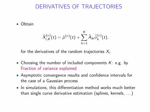
DERIVATIVES OF TRAJECTORIES
• Obtain
X (ν)i ,K (t) = µ(ν)(t) +
K∑k=1
Aik φ(ν)k (t).
for the derivatives of the random trajectories Xi .
• Choosing the number of included components K : e.g. byFraction of variance explained
• Asymptotic convergence results and confidence intervals forthe case of a Gaussian process
• In simulations, this differentiation method works much betterthan single curve derivative estimation (splines, kernels, . . .)

● ●●●
●●● ● ●●●●● ●●
●●
60 80 100 120 140 160
01
23
45
6
t (hours)
log(pr
ice)
● ●●●
●●● ● ●●●●● ●●
●●
60 80 100 120 140 160
0.00
0.02
0.04
t (hours)
log'(p
rice)
60 80 100 120 140 160
−0.00
3−0
.001
0.001
t (hours)
log''(p
rice)
●●● ●
60 80 100 120 140 160
01
23
45
6
t (hours)
log(pr
ice)
●●● ●
60 80 100 120 140 160
0.00
0.01
0.02
0.03
0.04
t (hours)
log'(p
rice)
60 80 100 120 140 160
−0.00
3−0
.001
0.001
t (hours)
log''(p
rice)
Fitted price trajectories and their first two derivatives for twoauctions.

DYNAMICS OF GAUSSIAN PROCESSES
From the Karhunen-Loève representation of processes X , obtain forthe covariance function for derivatives
cov{X (ν1)(t),X (ν2)(s)} =∞∑
k=1
λkφ(ν1)k (t)φ
(ν2)k (s), ν1, ν2 ∈ {0, 1}, s, t ∈ T .
Assuming Gaussianity of X ,(X (1)(t)− µ(1)(t)
X (t)− µ(t)
)=
( ∑∞k=1 Akφ
(1)k (t)∑∞
k=1 Akφk(t)
)
∼ N2
((00
),
( ∑∞k=1 λkφ
(1)k (t)2 ∑∞
k=1 λkφ(1)k (t)φk(t)∑∞
k=1 λkφ(1)k (t)φk(t)
∑∞k=1 λkφk(t)2
))

EMPIRICAL DIFFERENTIAL EQUATION
Population level: E{X (1)(t)− µ(1)(t) | X (t)} = β(t){X (t)− µ(t)}
Subject level:
X (1)(t)− µ(1)(t) = β(t){X (t)− µ(t)}+ Z (t), t ∈ T ,
with varying coefficient function
β(t) =cov{X (1)(t),X (t)}
var{X (t)}=
∑∞k=1 λkφ
(1)k (t)φk(t)∑∞
k=1 λkφk(t)2
=12
ddt
log[var{X (t)}], t ∈ T ,
and Gaussian drift process Z .
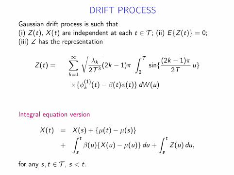
DRIFT PROCESSGaussian drift process is such that(i) Z (t), X (t) are independent at each t ∈ T ; (ii) E{Z (t)} = 0;(iii) Z has the representation
Z (t) =∞∑
k=1
√λk
2T 3 (2k − 1)π
∫ T
0sin{(2k − 1)π
2Tu}
×{φ(1)k (t)− β(t)φ(t)} dW (u)
Integral equation version
X (t) = X (s) + {µ(t)− µ(s)}
+
∫ t
sβ(u){X (u)− µ(u)} du +
∫ t
sZ (u) du,
for any s, t ∈ T , s < t.

LEARNING GAUSSIAN DYNAMICS
• For varying coefficient function β use plug-in estimates
β(t) =
∑Kk=1 λk φ
(1)k (t)φk(t)∑K
k=1 λk φ2k(t)
.
• dynamic regression to the mean (negative β)
• dynamic exponential growth (positive β)
• Interpretation within population modelE{X (1)(t)− µ(1)(t) | X (t)} = β(t){X (t)− µ(t)}

For drift process Z
var(Z (t)) =(∑k λk(φ
(1)k (t))2∑
k λkφ2k(t)− {
∑∞k=1 λkφ
(1)k (t)φk(t)}2
)/∑
k λkφ2k(t),
andvar{X (1)(t)} = β(t)2var{X (t)}+ var{Z (t)}.
Then the fraction of the variance of X (1)(t) explained by thedeterministic part of the differential equation is given by:
R2(t) =var{β(t)X (t)}var{X (1)(t)}
={∑∞
k=1 λkφ(1)k (t)φk(t)}2∑∞
k=1 λkφk(t)2∑∞
k=1 λkφ(1)k (t)2
.

100 110 120 130 140 150 160
−0.2
−0.18
−0.16
−0.14
−0.12
−0.1
−0.08
−0.06
−0.04
−0.02
0
Time (hour)
De
yn
am
ic t
ra
nsfe
r f
un
ctio
n β
(t)
100 110 120 130 140 150 160
−0.3
−0.25
−0.2
−0.15
−0.1
−0.05
0
0.05
0.1
0.15
0.2
Time (hour)E
ige
nfu
nctio
ns o
f Z
(t)
Left: Smooth estimate of the dynamic varying coefficient functionβ for auction data. Right: Smooth estimates of the first (solid),second (dashed) and third (dash-dotted) eigenfunction of driftprocess Z .

100 110 120 130 140 150 160
0
2
4
6
8
10
x 10−4
Time (hour)
Variance functions o
f X
(1) (
t) a
nd Z
(t)
100 110 120 130 140 150 1600
0.1
0.2
0.3
0.4
0.5
0.6
0.7
0.8
0.9
1
Time (hour)R
2(t
)
Left: Smooth estimates of the variance functions of X (1)(t)(dashed) and Z (t) (solid). Right: Smooth estimate of R2(t), thevariance explained by the deterministic part of the dynamicequation at time t.

−2 −1.5 −1 −0.5 0 0.5
−0.02
−0.01
0
0.01
0.02
0.03
0.04
0.05
Regression at t=125
Centered Xi(125)
Cen
tere
d X
i(1) (1
25)
−2 −1.5 −1 −0.5 0 0.5
−0.02
−0.01
0
0.01
0.02
0.03
0.04
0.05
Regression at t=161
Centered Xi(161)
Cen
tere
d X
i(1) (1
61)
Regression of X (1)i (t) on Xi (t) (both centered) at t = 125 hours
(left panel) and t = 161 hours (right panel), respectively, withregression slopes β(125) = −.015 and coefficient of determinationR2(125) = 0.28, respectively, β(161) = −.072 and R2(161) = 0.99.

45 50 55 60 65 70−0.03
−0.025
−0.02
−0.015
−0.01
−0.005
0β
Age (years)
Smooth estimate of the dynamic varying coefficient function β forBody Mass Index (BLSA).

45 50 55 60 65 70−0.005
0
0.005
0.01
0.015
0.02
0.025β
Age (years)
Smooth estimate of the dynamic varying coefficient function β forSystolic Blood Pressure (BLSA).

LEARNING DYNAMICS – NON-GAUSSIAN CASE• Data Model. For n realizations Xi of an underlying process X ,have Ni measurements Yij (i = 1, . . . , n, j = 1, . . . ,Ni ),
Yij = Yi (tij) = Xi (tij) + εij ,
with iid zero mean finite variance measurement errors εij .
• Linear Gaussian Dynamics. As before, with varying coefficientfunction β,
X ′(t) = µX ′(t) + β(t){X (t)− µX (t)}+ Z2(t),
where Z2 is a zero mean drift process withcov{Z2(t),X (t)} = 0.
• General Dynamics. There always exists a function f with
E{X ′(t) | X (t)} = f {t,X (t)}, X ′(t) = f {t,X (t)}+ Z (t) ,
with E{Z (t) | X (t)} = 0 almost surely and where f isunknown. Learning dynamics corresponds to inferring f .

• Special Case: Autonomous Dynamics.
E{X ′(t) | X (t)} = f1(X (t)), f1 unknown
• Parametric Dynamics. Parametric differential equations
X ′i (t) = g{t,Xi (t), θi}
require extensive knowledge of underlying system – oftenincorrect and hard to fit. Not much known for incorporatingrandom effects θi .

BERKELEY LONGITUDINAL GROWTH STUDY
• Dynamics of Human Growth of Interest
• Nonlinear Parametric Models: Preece-Baines, Triple-LogisticSubject-by-subject fitting, limited efficiency
• Berkeley Growth Study – 54 girls with 31 height measurementsfor ages 1 to 18, recorded at different time intervals, rangingfrom three months (from 1 to 2 years old), six months (from 8to 18 years old), to one year (from 3 to 8 years old).
• Learning dynamics:– Gain a better understanding of the growth process.– Distinguish between normal and pathological patterns ofdevelopment.

2 4 6 8 10 12 14 16 18
80
100
120
140
160
180
Age:yr
Est
ima
ge
d X
(t)
2 4 6 8 10 12 14 16 18
0
5
10
15
Age:yrE
stim
ate
d V
elo
city
: cm
/yr
Left panel: Estimated growth curves for 54 girls. Right panel: Estimatedgrowth velocity trajectories for 54 girls.

ESTIMATING THE DRIVING FUNCTION fAdopt a two-step kernel smoothing approach to obtain an estimator for fin E{X ′(t) | X (t)} = f {t,X (t)}:• Step 1: Obtaining estimates for X (t) and X ′(t):
Xi (t) =1
hX
Ni∑j=1
∫ sj
sj−1
YijK(
u − thX
)du,
X ′i (t) =1
h2X ′
Ni∑j=1
∫ sj
sj−1
YijK2
(u − thX ′
)du,
where sj = (tij + ti,j+1)/2 and hX > 0 and hX ′ > 0 are smoothingbandwidths.
• Step 2: Trajectory estimates X (t) and X ′(t) from Step 1 arecombined to obtain a Nadaraya–Watson kernel estimator for f ,
f (t, x) =
∑ni=1 K{ Xi (t)−x
bX}X ′i (t)∑n
i=1 K{ Xi (t)−xbX}
.
utilizing bandwidths bX > 0.
• Under regularity conditions, this gives consistent estimators.

Left panel: Estimated surface f (t, x) on a curved domain, characterizingthe deterministic part of the nonlinear dynamic model. Right panel:Contour plot of the surface f (t, x).

DECOMPOSING VARIANCE
• Since var{X ′(t)} = var[f {t,X (t)}] + var{Z (t)}, onsubdomains where the variance of the drift process var{Z (t)}is small, the deterministic approximation
X ′(t) = f {t,X (t)} (t ∈ T ),
is reasonable. Then future changes of individual trajectoriesare easily predictable.
• Fraction of the variance of X ′(t) that is explained by thedeterministic part
R2(t) =var[f {t,X (t)}]
var{X ′(t)}= 1− var{Z (t)}
var{X ′(t)}.

• Quantify predictability by
S(t, x) =f 2(t, x)
E{X ′2(t) | X (t) = x}=
f 2(t, x)
f 2(t, x) + var{Z (t) | X (t) = x}.
When S(t, x) is close to one, then f 2(t, x) is large comparedto var{Z (t) | X (t) = x} and the process is well predictablewhen X (t) = x .
• Diagnostics for linearity. For the coefficient of determinationfor the linear dynamic model
R2L(t) =
var {β(t)X (t)}var{X ′(t)}
one expects that R2(t) ≥ R2L(t) On subdomains of T where
R(t) is close to RL(t), one may infer that the data-drivendifferential equation is reasonably linear.
5 10 15
−0.4
−0.2
0
0.2
0.4
0.6
Age: yr
Est
ima
ted
R2 (
t)
5 10 150
0.1
0.2
0.3
0.4
0.5
0.6
0.7
0.8
Age: yr
Est
ima
ted
R2 (
t)
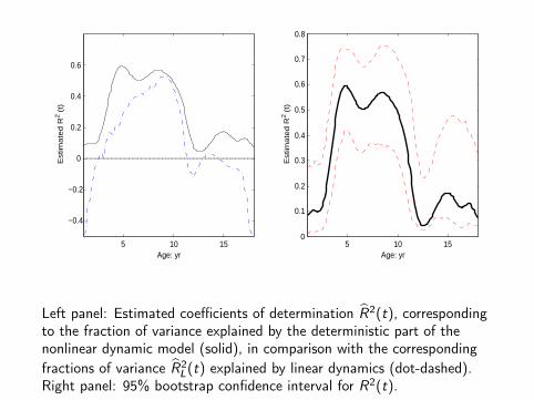
Left panel: Estimated coefficients of determination R2(t), correspondingto the fraction of variance explained by the deterministic part of thenonlinear dynamic model (solid), in comparison with the correspondingfractions of variance R2
L(t) explained by linear dynamics (dot-dashed).Right panel: 95% bootstrap confidence interval for R2(t).

• Linear concurrent model. Relating two stochastic processesX (t) and U(t) at each time t ∈ T , the linear concurrentmodel captures a linear relationship between X and U througha deterministic function β(t),
U(t) = µU(t) + β(t){X (t)− µX (t)}+ Z2(t),
where Z2(t) is a zero mean drift process withcov{Z2(t),X (t)} = 0.
• Nonlinear concurrent model. Proposed methodology coversthe case where the link between U(t) and X (t) is nonlinear,
U(t) = f {t,X (t)}+ Z (t) ,
with E{Z (t) | X (t)} = 0 almost surely andf {t,X (t)} = E{U(t) | X (t)}. Can establish consistency andrates of convergence for two-step estimators.
• Learning Gaussian dynamics works for sparse data, learningnon-Gaussian dynamics is viable only for dense data

75 80 85 90 958
9
10
11
12
13
14
152
height: cm
grow
th v
eloc
ity: c
m/y
r
90 100 110 1206
6.5
7
7.5
8
8.5
9
9.54
height: cm
grow
th v
eloc
ity: c
m/y
r
100 110 120 1305
5.5
6
6.5
7
7.5
8
8.56
height: cm
grow
th v
eloc
ity: c
m/y
r
110 120 130 140 1504.5
5
5.5
6
6.5
7
7.5
88
height: cm
grow
th v
eloc
ity: c
m/y
r
120 140 160 1803
4
5
6
7
812
height: cm
grow
th v
eloc
ity: c
m/y
r
150 160 170 180 190−0.5
0
0.5
1
1.5
2
2.5
316
height: cm
grow
th v
eloc
ity: c
m/y
r
Each of the panels, arranged for ages t = 2, 4, 6, 8, 12, from left to rightand top to bottom, respectively, illustrates estimates f (t, ·) of thedeterministic part of the nonlinear dynamic model (solid), the linearestimates (dashed) and the scatterplot of observed data pairs(x(t), x (1)(t)).

PART II
FUNCTIONAL REGRESSION

FUNCTIONAL REGRESSION MODELS
X 7→ YRd R Multiple Regression, GLMRd1 Rd2 Multivariate RegressionL2 R “Functional Predictor Models”Rd L2 “Functional Response Models”L2 L2 “Function to Function Regression”

MODELING FUNCTIONAL PREDICTORS
1. Functional Linear Regression
Idea: Extending the multivariate linear regression modelE (Y |X ) = BX to functional data (X (t),Y ) or (X (t),Y (t)):
E (Y |X ) = µY +
∫(X (s)− µX (s))β(s) ds,
the functional linear regression model with regression parameterfunction β and scalar responses (also generalized version byincluding link function (GFLM));
E (Y (t)|X ) = µY (t) +
∫(X (s)− µX (s))β(s, t) ds,
model with functional responses (Ramsay & Dalzell 1991;Grenander 1950)
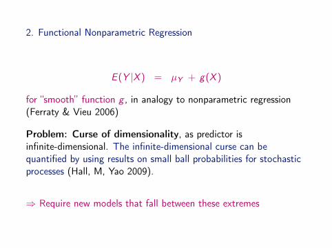
2. Functional Nonparametric Regression
E (Y |X ) = µY + g(X )
for “smooth” function g , in analogy to nonparametric regression(Ferraty & Vieu 2006)
Problem: Curse of dimensionality, as predictor isinfinite-dimensional. The infinite-dimensional curse can bequantified by using results on small ball probabilities for stochasticprocesses (Hall, M, Yao 2009).
⇒ Require new models that fall between these extremes

PRINCIPAL COMPONENT REPRESENTATIONOF FUNCTIONAL LINEAR REGRESSION
With predictor representations
X (s) = µX (s) +∞∑
k=1
Akφk(s)
obtain from normal equations for the functional linear model (FLM)E (Y |X ) = µY +
∫β(s)(X (s)− µX (s))ds:
β(s) =∞∑
k=1
E (AkY )
E (A2k)
φk(s) =∞∑
k=1
βkφk(s),
implyingE (Y |X ) =
∑k
βkAk

• Estimation: Can directly apply PACE to obtain all neededestimates. Alternative: Representation of regression parameterfunction β by B-splines or other basis expansions(Cardot et al. 1999; James et al. 2001)
• Special features of functional linear regression with PACE:Perturbation theory directly applicable for asymptoticsFunctional regression diagnostics: Based on decomposition ofLinear Functional Regression into series of simple linearregressions on FPCs; e.g.,Functional Cook’s distance and Functional hat matrix (Chiou& M 2007)
• Choice of included predictor components: Nested sequence,can use AIC-type criteria

FUNCTIONAL RESPONSE MODELS• Response process with mean function µY , eigenfunctions ψmand functional principal component (FPC) scores Bm:
Y (t) = µY (t) +∞∑
m=1
Bmψm(t)
• Given covariates Z ∈ Rp, this suggests conditioning approach
E{Y (t)|Z} = µY (t) +∞∑
m=1
E (Bm|Z )ψm(t)
← µY (t) +M∑
m=1
ηm(Z )ψm(t)
with nonparametric or semiparametric (e.g., single index)regressions
ηm(Z ) = E (Bm|Z ).
• Mean response models:
E (Y (t)|Z = z) = µ(t, z)
Estimation nonparametrically though surface smoothing (M &Yao, 2006) or assuming structure for dimension reduction, e.g.

• Product Model:
µ(t, z) = µY (t)θ(z), E{Y (t)} = µY (t), E{θ(Z )} = 1,
product form is motivated empirically (Chiou et al. 2004)• Alternative: Functional ANOVA (Brumback & Rice 1998).

0 5 10 150
5
10
15
20
25
0 5 10 150
5
10
15
20
25

Least squares solution:
θ(z) = argminθ{∫
T[E (Y (t)|Z = z)− µ0(t)θ]2 dt},
implies
θ(z) =
∫µ0(t)E (Y (t)|Z = z) dt∫
µ20(t) dt
.
Add single index assumption: θ(z) = µ1(γ′z) for a smooth functionµ1 and a vector γ, |γ| = 1.Consequence of above: E{µ1(γ′Z )} = 1.

FUNCTIONAL DOSE-RESPONSEMedfly (Ceratitis capitata) experiments on reproductive behavior inresponse to nutrition amount (Carey laboratory at UC Davis).Predictor is amount of protein in diet, between 30 and 100%,response is daily egg-laying profile (n = 874,m = 10 dose levels)


d = 100 %
0 10 20 30 40 50 60 70 80
0
10
20
30
40
50
Age (Days)
Nu
mb
er
of
Eg
gs
d = 75 %
0 10 20 30 40 50 60 70 80
0
10
20
30
40
50
Age (Days)
Nu
mb
er
of
Eg
gs
d = 50 %
0 10 20 30 40 50 60 70 80
0
10
20
30
40
50
Age (Days)
Nu
mb
er
of
Eg
gs

l l
l
l
l
l l
l l
l
ll
l
l
l l
l
l
ll
l
l
l
l
l
l
ll
l
l
l
l
l
ll l l
l
l
l
0 10 20 30 40
05
10
15
20
25
30
Age (Days)
mu
0
ll
l
l
l
l
l
l
l
l
l
l
ll
l
l
ll
l
l
l
l
l
l
l
l
l
ll
l
l
l
l
l
l
l
l
l
l
l
ll
l
l
l
ll
l
l
ll
l
l
l
l
l
l
l
l
l
l
l
l
l
l
l
l
ll
l
l
l
l
l
l
l
l
l
ll
l
l
l
l
l
l
l
l
l
l
l
l
l
l
l
l
l
l
l
l
l
l
l
l
l
l
ll
l
l
l
ll
l
ll
l
l
l
l
l
l
l
lll
l
l
l
l
l
l
l
l
l
l
l
ll
l
l
l
l
l
lll
l
l
l
l
l
l
l
l
l
l
l
l
l
l
ll
l
l
l
l
l
l
l
l
l
ll
l
l
l
l
l
l
l
ll
l
l
l
l
l
l
l
l
l
l
l
l
l
l
l
l
l
l
l
l
l
l
l
l
l
l
l
l
l
l
l
l
l
l
l
l
l
l
l
l
l
l
l
l
l
l
l
l
l
lll
l
l
l
l
l
l
l
l
l
ll
l
l
l
l
l
l
l
l
ll
l
l
l
l
ll
l
l
ll
l
l
l
l
l
l
l
l
l
l
l
l
l
l
l
l
l
l
l
l
l
l
l
l
l
l
l
l
l
lll
l
l
l
l
l
l
l
ll
l
l
l
l
l
l
l
l
ll
l
l
l
l
l
l
l
l
l
l
l
l
l
l
l
l
l
l
l
l
l
l
l
ll
l
l
l
l
l
l
l
l
l
l
l
l
l
l
l
l
l
l
l
l
l
l
ll
l
l
l
ll
l
l
l
l
l
l
l
l
l
l
l
l
l
l
ll
l
l
l
l
l
l
l
l
l
l
l
l
l
l
l
l
l
l
l
l
l
l
l
l
l
lll
l
l
l
l
l
l
l
l
l
l
l
l
ll
l
l
l
l
l
l
l
ll
l
l
l
l
l
l
l
l
l
l
l
l
l
l
l
l
l
ll
l
l
l
l
l
l
l
ll
l
l
l
l
l
l
l
l
l
lll
lllll
ll
l
l
l
l
l
l
l
l
l
l
l
l
l
l
l
l
lll
l
l
l
l
l
l
l
l
l
l
l
l
ll
l
l
l
l
l
l
l
l
l
l
l
l
l
l
ll
l
l
l
l
l
l
l
l
l
l
l
l
l
l
l
l
l
ll
l
ll
l
l
ll
l
l
l
l
l
l
ll
l
l
l
l
ll
l
l
l
l
l
l
l
l
ll
l
l
l
l
l
l
l
l
l
l
l
l
l
l
ll
l
l
l
l
l
l
l
l
l
l
l
l
l
l
l
l
l
l
l
l
l
l
l
l
l
l
l
l
l
l
ll
l
l
l
l
l
ll
l
l
l
l
l
l
l
ll
l
l
l
l
l
l
l
l
l
l
l
ll
l
l
l
l
l
l
ll
l
ll
l
ll
l
l
l
l
l
l
l
l
l
l
l
l
l
l
l
l
l
l
l
l
l
l
l
l
l
l
l
l
l
l
l
ll
l
l
l
l
l
l
l
l
ll
l
l
l
l
l
l
l
l
l
ll
l
l
ll
l
l
ll
l
l
l
ll
l
ll
l
l
l
l
ll
l
l
ll
l
l
l
ll
lll
l
l
l
l
l
l
l
l
l
l
l
l
l
l
l
ll
l
ll
l
l
l
l
ll
l
l
l
l
l
l
l
ll
l
l
l
l
l
l
l
l
l
l
l
l
l
l
l
l
ll
l
l
l
l
l
l
l
ll
l
l
l
l
l
l
l
lll
l
l
l
l
l
l
l
l
l
l
l
l
l
l
ll
l
l
l
l
l
l
l
l
l
ll
l
l
l
l
l
l
l
l
l
l
l
l
0.5 0.6 0.7 0.8 0.9 1.00
.00
.51
.01
.5
Treatment Dose Level
mu
1
Function estimates of the mean function and multiplicative components, with overall mean function
µ0(t) (left) and multiplicative effect function µ1(z) (right).

0 10 20 30 40
-0.3
-0.2
-0.1
0.0
0.1
0.2
0.3
Time (Days)
1st E
ige
nfu
nctio
n
0 10 20 30 40
-0.3
-0.2
-0.1
0.0
0.1
0.2
0.3
Time (Days)
2n
d E
ige
nfu
nctio
n
0 10 20 30 40
-0.3
-0.2
-0.1
0.0
0.1
0.2
0.3
Time (Days)
3rd
Eig
en
fun
ctio
nThe first three estimated eigenfunctions {ψk}k=1,...,3. The first eigenfunction explains 35.31%, the
second additional 16.84%, and the third additional 8.82% of total variation.

FLM FOR FUNCTIONALPREDICTORS AND RESPONSES
Extending the multivariate linear regression model E (Y |X ) = BXto functional data (X (t),Y (t)):
E (Y (t)|X ) = µ(t) +
∫X (s)β(s, t) ds.
Estimation of the parameter function β(·, ·) is an inverse problem.

• Idea: Extending the least squares normal equationcov(X ,Y ) = cov(X )B.
• “Functional Normal Equation” (He et al. 2000,2003)For auto-covariance operator AG of predictors X and
rXY (s, t) = cov [X (s),Y (t)] : rXY = AGβ.
• Since AG is a compact operator in L2, equation is notinvertible. Require functional generalized inverse: Well-definedunder regularity conditions and obtained by regularization –truncation of included components or penalty (Cai & Hall2006, Hall & Horwitz 2007).

Solution of the functional normal equation:
β∗(s, t) =∞∑
j ,k=1
cov(ξj , ζk)
var(ξj)ϕj(s)ψk(t).
Practical solution: By discretization.
Existence of solution in image space of AG .

REPRESENTATIONS OF FLR
With predictor and response representations
X (s) = µX (s) +∞∑
k=1
Akφk(s), Y (t) = µY (t) +∞∑
m=1
Bmψm(t)
obtain from normal equations for the modelE (Y (t)|X ) = µY (t) +
∫β(s, t)(X (s)− µX (s))ds
the representation
β(s, t) =∞∑
m=1
∞∑k=1
E (AkBm)
E (A2k)
φk(s)ψm(t) =∞∑
m=1
∞∑k=1
βmkφk(s)ψm(t)
which implies E (Bm|X ) =∑βmkAk and (as Ak are uncorrelated)
E (Bm|Ak) = E [E (Bm|A1,A2, . . .)|Ak ] = E [E (Bm|X )|Ak ] = βmkAk .

NOTES
• Other basis representations (wavelets, B-splines) have beenconsidered, eigen-representation has advantages due touncorrelatedness of scores (independence in Gaussian case)and (relative) sparseness of representation (often only few basefunctions needed, especially for prediction purposes)
• Obtaining estimated FPC scores Ak , Bm through the PACEmethod (Yao et al 2005), then βmk = cov(Ak , Bm)/λk , ie, allit takes is a series of simple linear regressions through theorigin.
• Inference: Simultaneously sample predictor and response datafor randomly resampled subjects, then recalculate functionalregression and obtain bootstrap confidence regions.
• Alternatively, separately resample predictor and response dataand obtain bootstrap distribution of suitable statistic undernull hypothesis of no functional relationship.

DROSOPHILA LIFE CYCLE GENE EXPRESSION
Consider gene time course data, where gene expression isrepeatedly measured for:
• 23 “muscle specific” genes: tissue-specific, muscle development• 22 “skeleto-neural” genes

0 10 20 30 40 50 60−4
−3
−2
−1
0
1
2
3
4
5Embryo Larva Pupa Adult
Time Unit
Gen
e E
xpre
ssio
n Le
vel
A subset of observed gene expression profiles (strict maternal genes). Each profile (or curve) is
composed of expression levels of one gene at different time points.

5 10 15 20 25 30−5
−4
−3
−2
−1
0
1
2
3
4
5
Time Unit (s)
Obs
erve
d Tr
ajec
torie
s/M
ean
Func
tion
of X
mean
trajectories
5 10 15 20 25−5
−4
−3
−2
−1
0
1
2
3
4
5
Time Unit (t)
Obs
erve
d Tr
ajec
torie
s/M
ean
Func
tion
of Y
mean
trajectories
Observed trajectories and estimated mean function for muscle-specific genes for predictor profiles X
(corresponding to gene expression profiles in embryo phase, left panel) and for response profiles Y
(profiles for pupa-adult phase, right panel)

5 10 15 20 25 30−0.3
−0.2
−0.1
0
0.1
0.2
0.3
0.4
Time Unit (s)
FPC
Fun
ctio
ns o
f X
j=1 (78.0%)
j=2 (20.5%)
5 10 15 20 25−0.3
−0.2
−0.1
0
0.1
0.2
0.3
0.4
0.5
Time Unit (t)
FPC
Fun
ctio
ns o
f Y
k=1 (75.7%)
k=2 (16.8%)
First two estimated eigenfunctions for temporal gene expression trajectories for the muscle-specific genes
in embryo phase (predictors X , left panel) and pupa-adult phase (responses Y , right panel).

−10 −5 0 5 10−4
−2
0
2
4
6
8
FPCs of X (j=1)
FPC
s of
Y (k
=1)
−10 −5 0 5−4
−2
0
2
4
6
8
FPCs of X (j=2)
FPC
s of
Y (k
=1)
−10 −5 0 5 10−3
−2
−1
0
1
2
3
FPCs of X (j=1)
FPC
s of
Y (k
=2)
−10 −5 0 5−3
−2
−1
0
1
2
3
FPCs of X (j=2)
FPC
s of
Y (k
=2)
Scatterplots of functional principal component scores ζk of response trajectories versus ξj of predictor
trajectories, for j, k = 1, 2, for muscle-specific genes

010
2030
0
10
20
−0.04
−0.02
0
0.02
0.04
0.06
Time Unit of X (s)Time Unit of Y (t)
β(s,
t)
Estimated regression parameter function β(s, t) for muscle-specific genes with embryo phase as predictor
X (s) (plotted towards the right) and pupa-adult phase as response Y (t) (plotted towards the left)

FUNCTIONAL COEFFICIENT OF DETERMINATIONAND DIAGNOSTICS
Extension from the multiple linear regression case:
R2 =
∫T var(E [Y (t)|X ])dt∫T var(Y (t))dt
=∞∑j=1
∑∞k=1 R2
kjτk∑∞k=1 τk
,
where
R2kj =
[cov(ξj , ζk)]2
λjτk
are the coefficients of determination for the simple linearregressions of ζk on ξj . Obtain estimate R2 = 0.85 formuscle-specific genes (p = 0.0010 from bootstrap test)Functional diagnostics can be obtained by a similar weightingscheme: Functional hat matrix, functional Cook’s distance, etc.

5 10 15 20 25 30−3
−2
−1
0
1
2
3
4
Time Unit (s)
Obs
erve
d Tr
ajec
torie
s/M
ean
Func
tion
of X
mean
trajectories
5 10 15−4
−3
−2
−1
0
1
2
3
Time Unit (t)
Obs
erve
d Tr
ajec
torie
s/M
ean
Func
tion
of Y
mean
trajectories
Observed trajectories and estimated mean function for cytoskeleton/neural genes in embryo phase (for
predictor X , left panel) and pupa phase (for response Y , right panel), respectively. Trajectories of gene
CG2198 are dashed.

0 5 10 15 200
0.1
0.2
0.3
0.4
0.5
0.6
0.7
0.8
0.9
Func
tiona
l Lev
erag
es
Index0 5 10 15 20
0
0.05
0.1
0.15
0.2
0.25
0.3
0.35
0.4
Func
tiona
l Coo
k’s
Dis
tanc
es
Index
Functional leverages obtained as diagonal elements of functional hat matrix H (left panel) and
functional Cook’s distances (right panel) for the functional regression of cytoskeleton/neural genes.

FUNCTIONAL LINEAR MODELFOR LONGITUDINAL DATA
Regress processes Y (·) on processes X (·) under sparse datasituation. Notation:Xi (s) on [0,S] : smooth predictor curve
Uil : measurements of Xi (·) at Sil , 1 ≤ i ≤ n, 1 ≤ l ≤ Li
Yi (t) on [0, T ] : smooth response curve
Vij : measurements of Yi (·) at Tij , 1 ≤ j ≤ Ni

Functional Regression Model
E [Y (t)|X (·)] = µY (t) +
∫ S0β(s, t)X (s)ds.
β(s, t) : smooth regression function,∫ T0
∫ S0 β2(s, t)dsdt <∞.
Modelling Predictor and Response Curves:
Uil = Xi (Sil ) + eil = µX (Sil ) +∞∑
m=1
Aimφm(Sil ) + eil ,
Vij = Yi (Tij) + εij = µY (Tij) +∞∑
k=1
Bikψk(Tij) + εij .

BASIS REPRESENTATION
β(s, t) =∞∑
k,m=1
E [AmBk ]
E [A2m]
φm(s)ψk(t)
Estimating E [AmBk ]:
E [AmBk ] =
∫ T0
∫ S0φm(s)ΓXY (s, t)ψk(t)dsdt,
where ΓXY (s, t) is local linear smoothing estimate of the covariancesurface ΓXY (s, t) = cov(X (s),Y (t)).

CONDITIONAL METHOD
Objective: Predict trajectory Y ∗ of a new subject, givenobservations U∗ = (U∗1 , · · · ,U∗L∗)T of X ∗(·).
E [Y ∗(t)|X ∗(·)] = µY (t) +
∫ S0β(s, t)X ∗(s)ds
= µY (t) +∞∑
k,m=1
E [AmBk ]
E [A2m]
A∗mψk(t)
Constraint: µY (t) =∫ S0 β(s, t)µX (s)ds.

PREDICTION OF Y ∗(t)
Y ∗KM(t) = µY (t) +M∑
m=1
K∑k=1
E [AmBk ]
E [A2m]
E [A∗m|U∗]ψk(t),
where E [A∗m|U∗] is estimated by the conditional method, givenobservations U∗ = (U∗1 , · · · ,U∗L∗)T of X ∗(·).

ASYMPTOTICS FOR FUNCTIONAL LINEAR REGRESSION
Consistency for β(s, t) and YKM(t) under regularity conditionsPointwise Bands for Y (t)
Y ∗K ,M(t)± Φ(1− α/2)√ωKM(t, t)
Functional R2:
R2 =
∫T var(E [Y (t)|X ])dt∫T var(Y (t))dt
=
∑∞k,m=1 σ
2km/ρm∑∞
k=1 λk

APPLICATION
Functional Regression of Systolic Blood Pressure on Body MassIndex
Data: Body mass index (BMI) and systolic blood pressure (SBP)for 812 participants in the Baltimore Longitudinal Study on Aging
Irregular and Sparse MeasurementsR2 = 0.13

60 65 70 75 80
18
20
22
24
26
28
30
32
34
Age (years)
Bod
y M
ass
Inde
x (k
g/m
2 )
60 65 70 75 80
90
100
110
120
130
140
150
160
170
180
190
200
Age (years)
Sys
tolic
Blo
od P
ress
ure
(mm
Hg)
Observed paths of Body Mass Index (left) and Systolic Blood Pressure (right) for 812 participants.

60
65
70
75
80
60
65
70
75
80
−1
−0.5
0
0.5
1
s (years)t (years)
Estimated regression function β(s, t), where the predictor (BMI) time is s (in years), and the response
(SBP) time is t (in years).

60 65 70 75 80110
120
130
140
150
160
Age (years)
SB
P (m
m H
g)
60 65 70 75 80100
110
120
130
140
150
160
Age (years)
SB
P (m
m H
g)
60 65 70 75 80110
120
130
140
150
160
Age (years)
SB
P (m
m H
g)
60 65 70 75 80110
120
130
140
150
160
Age (years)
SB
P (m
m H
g)
Observed data (circles), predicted trajectories (black), 95% pointwise (blue) and simultaneous (red)
bands obtained by one-leave-out analysis.

GENERALIZED FUNCTIONAL LINEAR MODEL
• Predictors X (t) ∈ L2, Response Y ∈ R• Components: Parameter Function β(·), Link Function g(·),Variance Function σ2(·)
ηi = α +
∫β(t)Xi (t) dw(t) linear predictors
Yi = g(ηi ) + ei = µi + ei , i = 1, . . . , n,
with i.i.d. errors ei , means E (Yi ) = µi = g(ηi ) andE (e|X (·)) = 0, var(e|X (·)) = σ2(µ).

• If link function g(·) and variance function σ2(·) are unknownand smooth, they can be estimated from the data.
• Applications of generalized functional linear model (GFLM):For example in classification, when Y denotes classmembership and a binary link function (e.g., logistic link) isused.
• With orthonormal basis ϕj , j ≥ 1,
X (t) =∞∑j=1
ζjϕj(t), β(t) =∞∑j=1
βjϕj(t)
∫β(t)X (t) dw(t) =
∞∑j=1
βjζj .

ANALYSIS
Writing ζ(i)j =∫
Xi (t)ϕj(t)dw(t), consider a sequence ofpn-truncated models, pn →∞ as n→∞,
Y (pn)i = g
α +
pn∑j=1
βjζ(i)j
+ e ′i σ
α +
pn∑j=1
βjζ(i)j
, i = 1, . . . , n
with standardized errors e ′i .

ESTIMATING EQUATION
• Given p = pn, the solution of the quasi-score (estimating)equation
U(β) =n∑
i=1
(Yi − µi )g ′(ηi )ζ(i)/σ2(µi ) = 0
is the (p + 1)-vector β.• This is the quasi-likelihood estimator for fixed p, given asingle-index model with link function g , variance functionσ2(·) and predictors ζ(i)1 , . . . , ζ
(i)p .
• Solution is numerically obtained by iterative weighted leastsquares (Newton-Raphson).

ASYMPTOTICS
Define Γ = Γp = (γkl )0≤k,l≤p, γkl = E(
g ′2(η)σ2(µ)
ζkζl
).
Under regularity conditions, as n→∞:
Theorem. For pn-vectors β = (β1, . . . , βpn) and estimates β,
n(β − β)T Γpn (β − β)− (pn + 1)√2 pn
d→ N(0, 1).
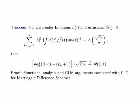
Theorem. For parameter functions β(·) and estimates β(·): If
∞∑j=pn+1
λGj [
∫β(t)ϕG
j (t) dw(t)]2 = o(√
pn
n
),
then [nd2
G (β, β)− (pn + 1)]/√
2 pnd→ N(0, 1).
Proof: Functional analysis and GLM arguments combined with CLTfor Martingale Difference Schemes.

FURTHER EXTENSIONS OF THE FLM“Classic” extensions: linear ⇒ quadratic ⇒ polynomial
The polynomial functional regression model (Yao & M 2010)
E (Y |X ) = α +
∫Tβ(t)X c(t)dt +
∫T 2γ(s, t)X c(s)X c(t)dsdt
+
∫T 3γ3(t1, t2, t3)X c(t1)X c(t2)X c(t3)dt1dt2dt3 + . . .
+
∫T pγp(t1, . . . , tp)X c(t1) . . .X c(tp)dt1 . . . dtp,
with α as intercept and β, γ, γj , 3 ≤ j ≤ p, as linear, quadraticand jth order regression parameter functions. In terms of FPCs,
E (Y |X ) = α +∑j1≥1
βj1Aj1 +∑j1≤j2
γj1j2Aj1Aj2 +∑
j1≤j2≤j3
γj1j2j3Aj1Aj2Aj3
+ . . . +∑
j1≤...≤jp
γj1...jpAj1 . . .Ajp ,
model includes all interaction effects up to p time points.

FUNCTIONAL QUADRATIC REGRESSION
E (Y |X ) = α +∞∑
k=1
βkAk +∞∑
k=1
k∑`=1
γk`AkA`,
Quadratic diagonal case
E (Y |X ) = α +∑k
βkAk +∑k
γkkA2k .
With eigenvalues λk for X and covariance functions
C1(t) = cov{X (t),Y } =∞∑
k=1
ηkφk(t),
C2(s, t) = E{X (s)X (t)Y } =∞∑
k,`=1
ρk`φk(s)φk(t),
least squares estimators are obtained via the representationsα = µY −
∑k γkkλk , βk = ηk/λk , γk` = ρk`/(λkλ`),
for k < `, γkk = (ρkk − µYλk)/(E (A4k)− λ2
k).

Can easily be implemented with PACE (quadreg, included inversion 2.12).
Asymptotics
Obtain consistent estimates and rates of convergence for parameterfunctions α− α = Op(αn), ‖β − β‖ = Op(βn), ‖γ − γ‖ = Op(γn)and for predicting new responses under either one of twoassumptions:
• Gaussian assumption on predictor processes X : Convergencerates for sparse irregular designs
• Densely observed functional predictors with noise; Gaussianassumption not needed for convergence rates
Note: The proofs for the two designs are quite different.

QUADRATIC FUNCTIONAL REGRESSION IN ACTION
0 10 20 30 40 50 60 70 80 90 1002
2.5
3
3.5
4
4.5
Spectrum Channel
Abso
rban
ce
Log-transformed absorbance spectra for Tecator fat contents data,for subset of 50 meat specimen (a Chemometrics test set)

0 20 40 60 80 1002.7
2.8
2.9
3
3.1
3.2
3.3
3.4
3.5
3.6
Spectrum Channel
Absorb
ance
0 20 40 60 80 100−0.25
−0.2
−0.15
−0.1
−0.05
0
0.05
0.1
0.15
0.2
Spectrum Channel
Eig
enfu
nctions
Mean function and four eigenfunctions for predictor processes

0 10 20 30 40 50 60 70 80 90 100−12
−10
−8
−6
−4
−2
0
2
4
6
8
Spectrum Channel
Lin
ear
Reg. T
erm
0
10
20
30
40
50
60
70
80
90
100
0
10
20
30
40
50
60
70
80
90
100
−2
−1
0
1
2
Spectrum ChannelSpectrum Channel
Quadra
tic R
eg. T
erm
Estimates of linear parameter function β (left) and quadraticregression parameter surface γ (right). Leave-out prediction errorsranking: QFM < Chemometrics-PLS < FLM.

−100
10
−1−0.500.5145
50
55
60
65
70
75
80
85
1st FPC2nd FPC
Fitte
d s
urf
ace
−10
0
10
−0.50
0.530
40
50
60
70
80
90
1st FPC3rd FPC
Fitte
d s
urf
ace
−10 −5 0 5 10
−0.20
0.240
50
60
70
80
90
1st FPC4rd FPC
Fitte
d s
urf
ace
−1
0
1
−0.50
0.540
45
50
55
60
65
70
75
80
85
2nd FPC3rd FPC
Fitte
d s
urf
ace
−1
0
1
−0.2−0.1
00.1
0.250
55
60
65
70
75
80
85
90
2nd FPC4th FPC
Fitte
d s
urf
ace
−0.50
0.5
−0.2−0.100.10.230
40
50
60
70
80
90
100
3rd FPC4th FPC
Fitte
d s
urf
ace
Sections through the fitted model E (Y |A1,A2,A3,A4).

AN ADDITIVE EXTENSION OF THEFUNCTIONAL LINEAR MODEL (FLM)
The least squares parameter function in the FLME (Y |X ) = µY +
∫β(s)(X (s)− µX (s))ds
has the representationβ(s) =
∑m∑
k βkφk(s) with βk = E (AkY )/E (A2k),
yieldingE (Y |X ) =
∑k
βkAk .
This motivates the following extension:Functional Additive Model
E (Y |X ) =∑k
fk(Ak),
where fk are smooth nonparametric functions; analogously forfunctional responses.

FUNCTIONAL ADDITIVE MODEL (FAM)Assuming independent predictor scores Aj (automatically implied inthe Gaussian case) we find
E (Y |Ak) = E{E (Y |X )|Ak} = E{∞∑j=1
fj(Aj)|Ak} = fk(Ak).
Consequence: Functional Additive Model can be implementedsimply by 1-d scatterplot smoothing of Y vs Aik to obtain thedefining functions fk .
No backfitting iteration is needed: Fast and straightforwardimplementation with PACE. Analogously for functional regressionmodel with scalar responses. For situations with several predictorfunctions within subjects: Can apply common additive model toensemble of selected FPCs for all predictor functions.

ASYMPTOTICS FOR FAM
Employing PACE, one may show under regularity conditions that fkis consistent for fk and the prediction E (Y |X ∗) is consistent forE (Y |X ∗) (M & Yao 2008)
Key steps for proof:
• Differences between Aik and Aik are asymptotically smallenough to be negligible for the FAM smoothing steps.
• Perturbation analysis for linear operators, bounding thedifference between operators AG and AG .
• In the dense design case, obtain essentially 1-d rates ofconvergence for the component functions fk .

ADDITIVE EXTENSION OF THEFUNCTIONAL RESPONSE MODEL
Consider FLM with functional responses, with FPC representationY (t) = µY (t) +
∑m Bmψm(t).
Then the least squares parameter function in the FLME (Y (t)|X ) = µY (t) +
∫β(s, t)(X (s)− µX (s))ds
has the representationβ(s, t) =
∑m∑
k βkmφk(s)ψm(t) with βkm = E (AkBm)/E (A2k)
yieldingE (Y (t)|X ) =
∑m
∑k
βmkAkψm(t).
This motivates the following extension:Functional Additive Model
E (Y (t)|X ) =∑m
∑k
fkm(Ak)ψm(t),
where fkm are smooth nonparametric functions.

FAM FOR FUNCTIONAL RESPONSESAssuming independent predictor scores Aj (automatically implied inthe Gaussian case) we find
E (Bm|Ak) = E{E (Bm|X )|Ak} = E{∞∑j=1
fjm(Aj)|Ak} = fkm(Ak).
Consequence: Functional Additive Model can be implementedsimply by 1-d scatterplot smoothing of Bim vs Aik to obtain thedefining functions fkm.
No backfitting iteration is needed: Fast and straightforwardimplementation with PACE. Analogously for functional regressionmodel with scalar responses. For situations with several predictorfunctions within subjects: Can apply common additive model toensemble of selected FPCs for all predictor functions.

0 5 10 15 20
−3
−2
−1
0
1
2
3
4
5
Time(hours)
Gen
e Ex
pres
sion
Lev
el
120 140 160 180 200
−3
−2.5
−2
−1.5
−1
−0.5
0
0.5
1
Time(hours)
Gen
e Ex
pres
sion
Lev
el
Gene time course data, zygotic genes for Drosophila for embryophase (left) and pupa phase (right).

0 5 10 15 20
−0.3
−0.2
−0.1
0
0.1
0.2
0.3
0.4
0.5
0.6
Time(hours)
Eigenfunctions of X
120 140 160 180 200−0.25
−0.2
−0.15
−0.1
−0.05
0
0.05
0.1
0.15
Time(hours)
Eigenfunctions of Y
First three eigenfunctions for embryo phase (predictor) and firstfour eigenfunctions for pupa phase (response).

Table: Functional R2, 25th, 50th and 75th percentiles and mean of thecross-validated observed relative prediction errors, RPE(−i),f , comparingFAM and functional linear regression models for zygotic data.
25th 50th 75th Mean R2
FAM .0506 .0776 .1662 .1301 0.19LIN .0479 .0891 .1727 .1374 0.16

0 5 10
−10
−5
0
5
−2 0 2
−10
−5
0
5
−1 0 1
−10
−5
0
5
0 5 10
−2
0
2
−2 0 2
−2
0
2
−1 0 1
−2
0
2
0 5 10−1.5−1
−0.50
0.5
−2 0 2−1.5−1
−0.50
0.5
−1 0 1−1.5−1
−0.50
0.5
0 5 10
−0.5
0
0.5
1
−2 0 2
−0.5
0
0.5
1
−1 0 1
−0.5
0
0.5
1
Scatterplots (dots), local polynomial (solid) and linear (dashed)estimates for the regressions of estimated FPC scores of the pupaphase (y-axis) versus those for the embryo phase (x-axis).

0 10 20−2
−1
0
1
2
Time(hours)
Pred
icto
r: Em
bryo
Pha
se
120 140 160 180 200
−2
−1.5
−1
−0.5
Time(hours)
Res
pons
e: P
upa
Phas
e
0 10 20−2
−1
0
1
2
Time(hours)
120 140 160 180 200
−2
−1.5
−1
−0.5
Time(hours)
0 10 20−2
−1
0
1
2
Time(hours)
120 140 160 180 200
−2
−1.5
−1
−0.5
Time(hours)
Changes of response functions as predictor functions change in thedirections of the first three eigenfunctions when fitting theFunctional Additive Model.

Further Examples of Functional Regression with PACEPACE Version 2.16, descriptions and references available athttp://anson.ucdavis.edu/∼mueller/data/pace.html
• FPCreg , FPCdiag : Let X c(t) = X c(t)− µ(t)
E (Y |X ) = α +
∫X c(t)β(t)dt
• FPCQuadReg : (Yao and Müller 2010, Horvath and Reeder, 2012)
E (Y |X ) = α +
∫X c(t)β(t)dt +
∫∫γ(s, t)X c(s)X c(t)dsdt
• FPCquantile (Chen and Müller 2012. JRSSB.)
P(Y ≤ y |X ) = E (I (Y ≤ y)|X ) = g−1(α(t)+
∫X c(t)β(y , t)dt)

Predictor Functions: Tecator Spectral Data
850 900 950 1000 10502
2.5
3
3.5
4
4.5
5
5.5
Spectrum Channel
Abs
orba
nce

Coefficient of Linear Regression
850 900 950 1000 1050−800
−600
−400
−200
0
200
400
600
800
1000
1200
x
Confidence bands for Beta
E (Y |X ) = α +∫
X c(t)β(t)dt

Residual Plot for Linear Regression
0 10 20 30 40 50 60
−10
−5
0
5
10
Fitted
Res
idua
l

Coefficients of Quadratic Regression
850 900 950 1000 1050−15
−10
−5
0
5
10
850
900
950
1000
1050
850
900
950
1000
1050
−2
−1
0
1
2
3
E (Y |X ) = α +∫
X c(t)β(t)dt +∫∫
γ(s, t)X c(s)X c(t)dsdt

Residual Plot for Quadratic Regression
0 5 10 15 20 25 30 35 40 45 50 55−5
−4
−3
−2
−1
0
1
2
3
4
5
Fitted
Res
idua
l

Quantiles
0 5 10 15 20 25 30 35 40 45 500
5
10
15
20
25
30
35
40
45
50
Fat Content
Pre
dict
ed Q
uant
iles
truemedian0.1 th0.9 th

Illustrative Example: Traffic Data

Velocity on I-880
21 22 23 24 25 26 27
10
20
30
40
50
60
70
10:25:26V
eloc
ity (
mph
)
21 22 23 24 25 26 27
10
20
30
40
50
60
70
14:15:41
21 22 23 24 25 26 27
10
20
30
40
50
60
70
16:33:50
Postmile
Vel
ocity
(m
ph)
21 22 23 24 25 26 27
10
20
30
40
50
60
70
12:29:56
Postmile

Prediction for Response Functions
• Y and X are both functions
• FPCfam: E (Y (t)|X ) = µY (t) +∑∞
k=1∑∞
j=1 fjk(ξk)ψj(t)
• FPCpredBands (Chen and Müller 2012): Global prediction bandsfor Y conditional on X
• For Gaussian process: E (Y |X ) and cov(Y |X )
• Common principal component assumptionAdditive assumption
cov(Y (t1),Y (t2) | X )= GYY (t1, t2) +
∑∞j=1{
∑∞k=1 gjk(ξk)−(∑∞
k=1 fjk(ξk))2}ψj(t1)ψj(t2)

Modeling the Prediction Bands
• Global prediction bands for Gaussian case:
P(µ(t)− DX (t) ≤ YX (t) ≤ µ(t) + DX (t) | X ) ≥ 1− α
where DX (t) = Cα {var(Y (t)|X )}1/2
• For more general random processes:
E {P(LX (t) ≤ YX (t) ≤ UX (t) | X )} ≥ 1− α
• Find Cα by the empirical coverage

‘Mobile Century’ Data
• Joint UC Berkeley - Nokia project (Herrera et al., 2010)
• Students were hired to drive on a segment of highway I-880and send data (time, location, and speed) back through GPSenabled mobile phones.
• The follow-up project ‘Mobile Millennium’ is generating moredata.

Estimated 90% Prediction Regions
0 50 100 150 200 250 300
−80−60−40−20
020
0 50 100 150 200 250 300
−80−60−40−20
020
0 50 100 150 200 250 300
−80−60−40−20
020
Rel
ativ
e S
peed
(m
ph)
0 50 100 150 200 250 300
−80−60−40−20
020
0 50 100 150 200 250 300
−80−60−40−20
020
Time (sec)0 50 100 150 200 250 300
−80−60−40−20
020
Time (sec)

FUNCTIONAL GRADIENTS
For functional linear regression with scalar responses:Derivative of an operator Γ : L2 → R at x =
∑k Axkφk is a linear
operator Γ(1)x : For functions u and scalars δ,
Γ(x + δu) = Γ(x) + δ Γ(1)x (u) + o(δ) as δ → 0.
The functional derivative operator at x is characterized by thefunctional directional derivatives
Γ(1)x (φk) = γxk ∈ R, k = 1, 2, . . .
in the directions of the basis functions φk .

Representation
Γ(1)x =
∞∑k=1
γxk Φk ,
where γxk = Γ(1)x (φk) is a scalar, and Φk denotes the linear
projection operator with
Φk(u) = Auk =
∫u(t)φk(t)dt, for all u ∈ L2(T ).

Example: Functional linear model. Representing the regressionparameter function β in the eigenbasis φk , β(t) =
∑k βkφk(t),
t ∈ T , leads to
ΓL(X ) = µY +∞∑
k=1
βkAXk = µY +∞∑
k=1
βkΦk(X ).
For any δ and arbitrary square integrable functions withrepresentations u =
∑k Aukφk and x =
∑k Axkφk ,
ΓL(x + δu) = µY +∑k
βk(Axk + δAuk) = ΓL(x) + δ∑k
βkAuk .
Then Γ(1)x =
∑∞k=1 βkΦk ⇒ γxk = βk . The functional
derivative does not depend on x , as Γ(1)x (φk) = βk .

ADDITIVE MODELING OF FUNCTIONAL GRADIENTS
Consider additive functional operatorΓA(X ) = E (Y c |X ) =
∑∞k=1 fk(AXk),
subject to Efk(AXk) = 0, k = 1, . . ., for FPC scores AXk .
For functions x =∑
k Axkφk and u =∑
k Aukφk ,
ΓA(x + δu) =∑k
fk(Axk + δAuk) = ΓA(x) + δ∑k
f (1)k (Axk)Auk + o(δ),
so that for the functional additive model,
Γ(1)A,x(u) =
∞∑k=1
f (1)k (Axk)Auk =∞∑
k=1
γA,xkΦk(u), γA,xk = f (1)k (Axk).

• Can easily extend to higher order derivatives due to additivestructure
• Asymptotics: For densely sampled functions, may obtainderivatives through derivative estimates of the additivefunctions, with the 1-d rates of convergence for derivativeestimation.

GRADIENTS FOR EGG-LAYING
• Predictor functions: Egg-laying trajectories (daily egg counts)for cohort of 818 female medflies (Carey et al. 98) that live≤ 20 days.
• Response: Lifetime fertility = total number of eggs laid overlifetime
• Preprocessing: Square root transformation of egg counts• Question: How do early reproductive trajectories influenceoverall reproductive success.
• Tools: Gradient field and its visualization

0 2 4 6 8 10 12 14 16 18 200
1
2
3
4
5
6
7
8
9
10
Time (days)
Pred
icto
r
Egg-laying trajectories (predictors, smoothed) for 50 randomlyselected flies, from a total of 818 medflies, for the first 20 days oftheir lifespan. Response=total eggs (reproductive success)

5 10 15 200
0.5
1
1.5
2
2.5
3
3.5
4
4.5
5
5.5
Time (days)5 10 15 20
−0.3
−0.2
−0.1
0
0.1
0.2
0.3
0.4
Time (days)
Smooth estimates of mean function (left panel) and first twoeigenfunctions (right panel) of the predictor trajectories, explaining72.1% (solid) and 18.6% (dashed) of the total variation,respectively.

−10 0 10
10
20
30
40
1st FPC scores
Res
pons
e
−5 0 5 10
10
20
30
40
2nd FPC scores
−10 0 100.5
1
1.5
2
2.5
3
3.5
1st FPC scores
Der
ivat
ive
−5 0 5 10−1
−0.8
−0.6
−0.4
−0.2
0
2nd FPC scores
Top panels: Nonparametric regression of the response (totalfertility) on the first (left) and second (right) FPC scores ofpredictor processes. Bottom panels: Estimated derivatives of thesmooth regression functions.
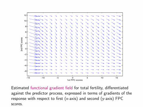
−15 −10 −5 0 5 10 15
−8
−6
−4
−2
0
2
4
6
8
10
12
1st FPC scores
2nd
FPC
sco
res
Estimated functional gradient field for total fertility, differentiatedagainst the predictor process, expressed in terms of gradients of theresponse with respect to first (x-axis) and second (y-axis) FPCscores.
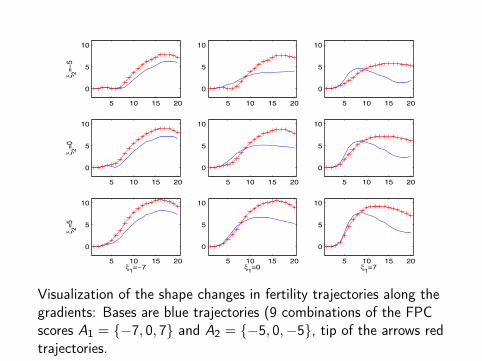
5 10 15 20
0
5
10
ξ 2=−5
5 10 15 20
0
5
10
5 10 15 20
0
5
10
5 10 15 20
0
5
10
ξ 2=0
5 10 15 20
0
5
10
5 10 15 20
0
5
10
5 10 15 20
0
5
10
ξ 2=5
ξ1=−7
5 10 15 20
0
5
10
ξ1=0
5 10 15 20
0
5
10
ξ1=7
Visualization of the shape changes in fertility trajectories along thegradients: Bases are blue trajectories (9 combinations of the FPCscores A1 = {−7, 0, 7} and A2 = {−5, 0,−5}, tip of the arrows redtrajectories.

MODELING TIME-SPECIFIC RELATIONS
Consider X ,Y ∈ L2. Instead of modeling relation of entirefunctions X ,Y :
Time-specific relationship of response process level Y (t) on levelX (s) of predictor process usually of interest for s ≤ t (also forseveral predictor processes).
Nonparametric approach for fully observed functions: ObtainE (Y (s)|X (t)) using a smoothing approach for the observed datafor all pairs (s, t) (Yao & M 2006), e.g., E (Y (s)|X (s)) = g(X (s))
Linear approach for sparse and irregularly observed functions underjoint Gaussianity for (X ,Y ) (Yang & M 2010):

• For X (c) =∑
k Akφk , Y (c) =∑
m Bmψm, obtain
E (Y (c)(t)|X (s)) = γ(s, t)X (c)(s)
γ(s, t) = [∑
k∑
m E (AkBm)φk(s)ψm(t)]/[∑
k λk(φk(s))2].
• Derive consistent estimators for the function γ.
• Study dynamic longitudinal relationships by extending theserelations to derivatives of Y and X : “Empirical Dynamics”

40 45 50 55 60 65 7024
25
26
27
28
29
30
31
32
33
34
Age (years)
BMI
40 45 50 55 60 65 70105
110
115
120
125
130
135
140
Age (years)
SBP
The observed values of body mass index (BMI) (left panel) andsystolic blod pressure (SBP) (right panel) for three randomlyselected subjects from Baltimore longitudinal study on aging

40
45
50
55
60
65
70
4045
5055
6065
70
1
1.5
2
2.5
3
3.5
4
4.5
s (age in years)
t (age in years)
Estimated function γ(s, t), s ≤ t linking SBP levels (responseprocess Y (t)) with BMI levels (predictor process X (s)) through therelation E (Y (t)|X (s)) = µY (t) + γ(s, t)(X (s)− µX (s)).

CONCLUSIONS
1. There is a need for functional regression models that:
– are more flexible than the functional linear model;– avoid the curse of dimensionality that negatively affectsstructurally unconstrained models such as fullynonparametric approaches
– accommodate more complex situations such as severalpredictor functions.
– accommodate the modeling of functional gradients– accommodate time-specific relationships.
2. Functional principal component representations prove useful todefine and analyze such models and to represent random functionsas building blocks in more complex models.