lectures on representations of surface groups
TRANSCRIPT

Lectures onRepresentations
of Surface Groups
Notes of a course given inETH-Zurich Fall 2006,
and
Orsay Spring 2007-2008.
Francois LABOURIE 1
(Based on notes taken by Tobias HARTNICK)
April 18, 2017
1Univ. Paris-Sud, Laboratoire de Mathematiques, Orsay F-91405 Cedex; CNRS,Orsay cedex, F-91405, The research leading to these results has received funding fromthe European Research Council under the European Community’s seventh Frame-work Programme (FP7/2007-2013)/ERC grant agreement o FP7-246918

Chapter 1
Introduction
The purpose of this lecture series is to describe the representation variety – orcharacter variety– of the fundamental group π1(S) of a closed connected surfaceS of genus greater than 2, with values in a Lie group G. This character varietyis roughly defined to be
Rep(π1(S), G) := Hom(π1(S), G)/G,
where G acts on Hom(π1(S), G) by conjugation.These character varieties have been heavily studied in the context of gauge
theories – mainly in the case of compact groups – and hyperbolic geometrywhen G = PSL2(R) or G = PSL2(C).
We shall mainly be interested in these lectures on the topology of thesevarieties and their symplectic structure which was discovered by Atiyah–Bott–Goldman, setting aside their interpretation in the theory of Riemann surfaces.
In the preliminary chapters, we give a crash course on surfaces, vector bun-dles and connections. While there is no new material here, we insist on de-scribing very early both differential geometric and combinatorial aspects of theobjects that we are interested in.
These various point of view allow us to give several models of the charactervariety generalising the familiar picture about first cohomology groups beingdescribed alternatively using de Rham, Cech or simplicial cohomology or asthe space of homomorphisms of the fundamental group into R.
We then describe the smooth structure of these character varieties as well astheir tangent spaces. The understanding of the volume form on these tangentspaces requires us, following Witten, to introduce Reidemeister torsion.
When G = PSL2(R), we prove Milnor–Wood Inequality and discuss con-nected components of the character variety.
We finally introduce the symplectic structure on these character varietiesand prove Witten’s formula which compute their symplectic volume in the case
1
CHAPTER 1. INTRODUCTION 2
of a compact groups. We introduce two important algebras of observables, thefirst one consisting of Wilson loops or the other of spin networks and computetheir Poisson bracket, thus introducing Goldman algebra.
In the last chapter, we turn to the integrality of the symplectic form andthe relation with 3-manifolds and the Chern–Simons invariant.
Each chapter is closed by a section giving general references and furtherreadings.
These notes correspond to lectures given at ETH-Zurich and Orsay at abeginning graduate level. The students were supposed to have only elementaryknowledge of differential geometry and topology. It follows that these notesare quite informal: in the first chapters, we do not insist in the details of thedifferential geometric constructions and refer to classical textbooks, while inthe more advanced chapters, we are sometimes reduced to give proofs only inspecial cases hoping that it gives the flavor of the general proofs. A typicalexample is the study of the properness of the action by conjugation of G onHom(π1(S), G): while the general case requires a certain knowledge of algebraicgroups and their action on algebraic varieties, we only treat here the case ofG = SLn(R) resorting to elementary arguments on matrices.
None of the results presented here are new, but the presentation and proofssometimes differ from other exposition.
Tobias Hartnick had the difficult task of turning the chaos of my lecturesin some decent mathematics, and I heartily thank him for writing up the firstdraft of these notes, giving them much of their shape and consistence.
I would also like to thank the mathematics department of ETH and theInstitute for Mathematical Research (FIM) in Zurich for their invitation.
These notes would certainly not have existed without the comments andencouragement of Francois Laudenbach, who taught me symplectic geometrya long time ago. Similarly, I benefitted from many enlightning discussions,advices and comments from W. Goldman, whose mathematics have shapedthe subject and who deserves special thanks.
I would also like to thank M. Burger, I. Chatterji, O. Garcıa-Prada, S.Kerckhoff, N. Hitchin, A. Iozzi, J. Souto, D. Toledo, R. Wentworth for manyhelpful comments on the text or the references.

Contents
1 Introduction 1
2 Surfaces 62.1 Surfaces as 2-dimensional manifolds . . . . . . . . . . . . . . . . 6
2.1.1 Basic definitions . . . . . . . . . . . . . . . . . . . . . . . 62.1.2 Surfaces with boundary . . . . . . . . . . . . . . . . . . 72.1.3 Gluing surfaces . . . . . . . . . . . . . . . . . . . . . . . 9
2.2 Surfaces as combinatorial objects . . . . . . . . . . . . . . . . . 122.2.1 Ribbon graphs . . . . . . . . . . . . . . . . . . . . . . . 122.2.2 Classification of surfaces I: Existence . . . . . . . . . . . 18
2.3 The fundamental group of a surface . . . . . . . . . . . . . . . . 232.3.1 The fundamental group of a topological space . . . . . . 232.3.2 Cayley graph and presentation complex . . . . . . . . . . 262.3.3 Classification of surfaces II: Uniqueness . . . . . . . . . . 28
2.4 Combinatorial versions of the fundamental group . . . . . . . . 292.4.1 A combinatorial description using a ribbon graph . . . . 292.4.2 A combinatorial description of the fundamental group
using covers . . . . . . . . . . . . . . . . . . . . . . . . . 312.5 Cohomology of Surfaces . . . . . . . . . . . . . . . . . . . . . . 32
2.5.1 De Rham cohomology . . . . . . . . . . . . . . . . . . . 322.5.2 Ribbon graphs and cohomology . . . . . . . . . . . . . . 382.5.3 The intersection form . . . . . . . . . . . . . . . . . . . . 41
2.6 Comments, references and further readings . . . . . . . . . . . . 44
3 Vector bundles and connections 453.1 Vector bundles . . . . . . . . . . . . . . . . . . . . . . . . . . . 45
3.1.1 Definitions . . . . . . . . . . . . . . . . . . . . . . . . . . 453.1.2 Constructions . . . . . . . . . . . . . . . . . . . . . . . . 48
3.2 Vector bundles with structures . . . . . . . . . . . . . . . . . . . 493.2.1 Vector bundles over manifolds . . . . . . . . . . . . . . . 52
3.3 Connections . . . . . . . . . . . . . . . . . . . . . . . . . . . . . 53
3

CONTENTS 4
3.3.1 Koszul connection . . . . . . . . . . . . . . . . . . . . . . 543.3.2 Constructions . . . . . . . . . . . . . . . . . . . . . . . . 563.3.3 Gauge equivalence and action of the gauge group . . . . 563.3.4 Holonomy along a path . . . . . . . . . . . . . . . . . . . 573.3.5 Holonomy and linear differential equations . . . . . . . . 583.3.6 Curvature . . . . . . . . . . . . . . . . . . . . . . . . . . 593.3.7 Flat connections . . . . . . . . . . . . . . . . . . . . . . 593.3.8 Connections preserving structures . . . . . . . . . . . . . 603.3.9 The holonomy map of a flat connection . . . . . . . . . . 61
3.4 Combinatorial versions of connections . . . . . . . . . . . . . . . 623.4.1 Discrete connections on ribbon graphs . . . . . . . . . . 623.4.2 Local systems . . . . . . . . . . . . . . . . . . . . . . . . 63
3.5 Four models of the representation variety . . . . . . . . . . . . . 643.5.1 Flat connections and local systems . . . . . . . . . . . . 653.5.2 Local systems and representations . . . . . . . . . . . . . 663.5.3 Smooth and discrete connections . . . . . . . . . . . . . 67
3.6 Comments, references and further readings . . . . . . . . . . . . 68
4 Twisted Cohomology 694.1 De Rham version of twisted cohomology . . . . . . . . . . . . . 69
4.1.1 Motivation: variation of connection . . . . . . . . . . . . 694.1.2 De Rham version of the twisted cohomology . . . . . . . 72
4.2 A combinatorial version . . . . . . . . . . . . . . . . . . . . . . 764.2.1 The combinatorial complex . . . . . . . . . . . . . . . . 774.2.2 The Isomorphism Theorem . . . . . . . . . . . . . . . . . 784.2.3 Duality . . . . . . . . . . . . . . . . . . . . . . . . . . . 814.2.4 Proof of Theorem 4.1.7 . . . . . . . . . . . . . . . . . . . 84
4.3 Torsion . . . . . . . . . . . . . . . . . . . . . . . . . . . . . . . . 854.3.1 Determinants . . . . . . . . . . . . . . . . . . . . . . . . 854.3.2 An isomorphism between determinants . . . . . . . . . . 864.3.3 The torsion of a metric complex . . . . . . . . . . . . . . 874.3.4 The torsion of a flat metric connection . . . . . . . . . . 874.3.5 Torsion and symplectic complexes . . . . . . . . . . . . . 894.3.6 Parallel metric on bundles . . . . . . . . . . . . . . . . . 91
4.4 Comments, references and further readings . . . . . . . . . . . . 93
5 Moduli spaces 945.1 Moduli space and character variety . . . . . . . . . . . . . . . . 945.2 Topology and smooth structure . . . . . . . . . . . . . . . . . . 955.3 Proof of the Theorem 5.2.6 . . . . . . . . . . . . . . . . . . . . . 97
5.3.1 The Zariski closure of a group . . . . . . . . . . . . . . . 98

CONTENTS 5
5.3.2 More on the holonomy map . . . . . . . . . . . . . . . . 1025.3.3 The Zariski dense part is Zariski open and non-empty . . 1045.3.4 The action is proper . . . . . . . . . . . . . . . . . . . . 1065.3.5 The moduli space and its tangent space . . . . . . . . . . 1095.3.6 The complement of the Zariski dense part . . . . . . . . 109
5.4 Connected components . . . . . . . . . . . . . . . . . . . . . . . 1105.4.1 Connected components I: the compact case . . . . . . . 1105.4.2 Connected Components II : an invariant . . . . . . . . . 1125.4.3 Connected components III: Milnor-Wood inequality . . . 1135.4.4 Connected components IV: Goldman’s work . . . . . . . 117
5.5 Comments, references and further readings . . . . . . . . . . . . 117
6 Symplectic structure 1196.1 Universal connections and smooth structures . . . . . . . . . . . 119
6.1.1 Lifting Lemmas . . . . . . . . . . . . . . . . . . . . . . . 1196.1.2 Universal connections . . . . . . . . . . . . . . . . . . . . 120
6.2 The symplectic form . . . . . . . . . . . . . . . . . . . . . . . . 1226.3 Classical mechanics and observables . . . . . . . . . . . . . . . . 1236.4 Special observables I: Wilson loops and the Goldman algebra . . 1246.5 Special observables II: Spin networks . . . . . . . . . . . . . . . 129
6.5.1 An observable on the space of all flat connections . . . . 1306.5.2 Poisson bracket of spin network observables . . . . . . . 131
6.6 Volumes of moduli spaces . . . . . . . . . . . . . . . . . . . . . 1336.6.1 Witten’s formula . . . . . . . . . . . . . . . . . . . . . . 1336.6.2 Volume and the disintegrated measure . . . . . . . . . . 1346.6.3 Characters and the disintegrated measure . . . . . . . . 137
6.7 Comments, references and further readings . . . . . . . . . . . . 139
7 Three manifolds and integrality 1417.1 Integrality . . . . . . . . . . . . . . . . . . . . . . . . . . . . . . 141
7.1.1 The Cartan form . . . . . . . . . . . . . . . . . . . . . . 1427.1.2 Integrating the Cartan form . . . . . . . . . . . . . . . . 143
7.2 Boundary of 3-Manifolds and Lagrangian submanifolds . . . . . 1467.2.1 Submanifolds of the moduli space . . . . . . . . . . . . . 1477.2.2 Isotropic submanifold . . . . . . . . . . . . . . . . . . . . 1487.2.3 Chern–Simons invariants . . . . . . . . . . . . . . . . . . 1487.2.4 Chern Simons action difference and the symplectic form 151
7.3 Comments, references and further readings . . . . . . . . . . . . 154
Index 155

Chapter 2
Surfaces
In this introductory chapter, we give two definitions of surfaces. First as adifferential geometric object, then as a combinatorial object: a ribbon graph.We use this description first to give the classification of oriented surfaces thento describe the fundamental objects we are going to deal with in this book:the fundamental group and the cohomology in its various guises. The style ofthis chapter is that of a crash course mainly meant to settle ideas and notationfor the next chapters.
The main point of this introductory chapter is to go back and forth be-tween the two languages that we are going to use in the first chapters of thismonograph: differential geometry and combinatorics.
2.1 Surfaces as 2-dimensional manifolds
2.1.1 Basic definitions
In this section, we will recall the point of view of differential geometers onsurfaces.
Definition 2.1.1 A surface is a connected two-dimensional smooth manifold.
We assume that the reader is familiar with the definition of a manifold. Nev-ertheless, in order to fix ideas and notation, let us briefly discuss the definitionabove. We assume first that S is a metrisable topological space, in particularHausdorff. A two-dimensional chart for such a topological space S is a pair(U,ϕ) where U ⊂ S is an open subset and ϕ is a map from U to R2, whereV = ϕ(U) is open in R2 and ϕ is a homeomorphism onto its image. The mapϕ is called the coordinate of the chart. A collection of charts (Ui, ϕi) | i ∈ I
6

CHAPTER 2. SURFACES 7
is called an atlas for S if S =⋃Ui. An atlas is called smooth or C∞ (we use
these two expressions synonymously) if the coordinate changes
ϕi ϕ−1j : ϕj(Ui ∩ Uj)→ ϕi(Ui ∩ Uj)
are smooth functions for all i, j ∈ I. The reason to introduce a smooth atlas isthe desire to be able to talk about smooth functions on S. If smooth functionsexists, we definitely want the coordinates ϕi and their inverses ϕ−1
i to besmooth.
So let us just pretend that they are smooth.
If the notion of smooth functions is any good, then given a smooth functionϕ : S → R also the composition or the function seen in the chart
ϕ−1i ϕ : ϕi(Ui)→ R
should be smooth. But these are just functions from subsets of R2 to R andfor such functions we know what smoothness means. Thus we can just definea function ϕ to be smooth if the function seen in all charts is smooth. Infact, it suffices to check this for only one particular chart around each pointas we were clever enough to demand the coordinate changes to be smooththemselves. Thus we may talk about smooth functions on a surface like wemay talk about smooth functions on R2.
Obvious examples of surfaces are given by connected open subsets of R2.Indeed, if U ⊂ R2 and i : U → R2 is the inclusion map then (U, i) is asmooth atlas for U . Geometric intuition tells us that all these examples areoriented, while the Mobius strip (Figure 2.1) is not. One way to formalise thisis via the derivatives of the coordinate changes:
Definition 2.1.2 Let S be a surface with atlas (Ui, ϕi) | i ∈ I. The atlas iscalled oriented if the Jacobians
Jac(ϕi, ϕj) := det(D(ϕi ϕ−1j ))
are positive for any i, j ∈ I. By a slight abuse of language we then say that Sitself is oriented
2.1.2 Surfaces with boundary
In order to study surfaces, we shall often cut a surface into pieces along a curveor to glue two such pieces in order to obtain a new surface. The pieces occurringin such geometric operations are not surfaces in the sense of Definition 2.1.1.

CHAPTER 2. SURFACES 8
Figure 2.1: The Mobius strip
Thus, we need a more general definition in order to deal with these pieces aswell. For this, we need another model space. Let
H+ := (x, y) ∈ R2 | y ≥ 0
be the closed upper half plane. The upper half plane has a boundary
∂H+ := (x, y) ∈ R2 | y = 0
when considered as a subset of R2. Given a metrisable space S, a two-dimensional chart with boundary is a pair (U,ϕ) where U is an open subset ofS and ϕ : U → V is a homeomorphism onto an open subset V ⊂ H+, whichis again called the coordinate of the chart. The subset
∂U := ϕ−1(ϕ(U) ∩ ∂H+) ⊂ U
will be called the boundary of U. In order to define a smooth atlas of chartswith boundary, we need to define a notion of smoothness for functions betweenopen subsets of H+.
Definition 2.1.3 Let V1, V2 be open subsets of H+. A function f : V1 → V2 iscalled smooth if there exists an open subset V1 of R2 with V1 ∩H+ = V1. anda smooth function f : V1 → R2 such that f = f |V1.
An atlas of charts with boundary (Ui, ϕi) | i ∈ I is smooth if the coordinatechanges
ϕi ϕ−1j : ϕj(Ui ∩ Uj)→ ϕi(Ui ∩ Uj)
are smooth in the sense of Definition 2.1.3. Then we may define:

CHAPTER 2. SURFACES 9
Definition 2.1.4 A surface with boundary is a metrisable space S togetherwith a smooth atlas of charts with boundary.
We define in a similar fashion as before the notion of smooth functions ona manifold with boundary. In order to define the boundary of a surface withboundary one needs to prove the following lemma:
Lemma 2.1.5 Let S be a surface with boundary and let (U1, ϕ1), (U2, ϕ2) becharts with boundary of S. Suppose x ∈ ∂U1 ∩ U2, in other words x is aboundary point of U1. Then x ∈ ∂U2 is a boundary point of U2.
Exercise 2.1.6 Deduce Lemma 2.1.5 from the implicit function Theorem.
In fact boundary points are not only preserved by smooth maps but even bycontinuous maps. To see this, however, requires some algebraic topology. ByLemma 2.1.5 the notion of being a boundary point of a chart does not dependon the particular chart. Thus we may define:
Definition 2.1.7 Let S be a surface with boundary. A point x ∈ S is calleda boundary point of S if x ∈ ∂U for some (and hence any) chart (U,ϕ)containing it. The set of boundary points of S is denoted ∂S.
In order to glue surfaces along their boundaries we need to know how theylook like in a neighbourhood of a boundary component. This is described bythe following lemma:
Lemma 2.1.8 [Collar Lemma] Let M be a surface with boundary ∂M andc ⊂ ∂M a connected component. Then there exists a neighbourhood U of cin M and a diffeomorphism ψ : U → V onto a subset V ⊂ R2 of the formV ∼= c× [0, 1) mapping c onto c× 0.
The neighbourhood U will be called a collar neighbourhood or tubular neigh-bourhood of c. The proof of Lemma 2.1.8 is easy if one uses Riemannian geom-etry and in particular exponential charts. There is no short elementary proofthough and we omit the proof.
2.1.3 Gluing surfaces
Let S1, S2 be two surfaces with boundary. Let c1 and c2 be two diffeomorphiccomponents of ∂S1 and c2 of ∂S2. Intuitively, the gluing of the two surfacesalong these boundary components is depicted by Picture 2.3. We sketch the

CHAPTER 2. SURFACES 10
MU
∂M
Figure 2.2: A collar neighbourhood
Figure 2.3: Gluing two surfaces
formalisation of this gluing procedure now. Let notation be as above and letϕ : c1 → c2 be a diffeomorphism. We define a topological space
S1 ∪ϕ S2
called the gluing of S1 and S2 along ϕ as follows: on the disjoint union S1
∐S2
we consider the equivalence relation generated by
x ∼ y ⇔ y = ϕ(x)
for x ∈ c1, y ∈ c2. Then S1 ∪ϕ S2 is the quotient of S1
∐S2 by this equivalence
relation.
Exercise 2.1.9 Show that the space S1 ∪ϕ S2 is metrisable.

CHAPTER 2. SURFACES 11
An atlas for S1 ∪ϕ S2 is now constructed as the union of three subsets:Firstly, we take a smooth atlas (Ui, ϕi) | i ∈ I for S1 \ c1 and a smooth atlas(Uj, ϕj) | j ∈ J for S2 \ c2. Denote by i1 : S1 → S1 ∪ϕ S2, i2 : S2 → S1 ∪ϕ S2
the canonical inclusions. Then
(i1(Ui), ϕi i−11 ) | i ∈ I ∪ (i2(Uj), ϕj i−1
2 ) | j ∈ J
is an atlas for the complement of the gluing curve in S1 ∪ϕ S2. It remains toconstruct a chart around this gluing curve which is compatible with the chartsabove. For this we use Lemma 2.1.8: Let U1, U2 be collar neighbourhoods ofc1, c2, ψ1 a diffeomorphism from U1 onto c1× (−1, 0] (mapping c1 to c1×0)and ψ2 a diffeomorphism from U2 onto c2 × [0, 1) (mapping c2 to c2 × 0).We consider the open subset O := U1 ∪ϕ U2 of S1 ∪ϕ S2 and fix an embeddingι : c2 × (−1, 1) → R2. This is always possible as c2 is either an interval or acircle. We define coordinates for O by
ψ : O → R2, x 7→ι (ϕ, id) ψ1(x) if x ∈ U1
ι ψ2(x) if x ∈ U2.
Then one has:
Proposition 2.1.10 S1 ∪ϕ S2 is a surface with boundary with smooth atlasgiven by
(i1(Ui), ϕi i−11 ) | i ∈ I ∪ (i2(Uj), ϕj i−1
2 ) | j ∈ J ∪ O,ψ.
Exercise 2.1.11 Prove Proposition 2.1.10.
Exercise 2.1.12 Let S1, S2 be oriented surfaces with boundary and c1, c2 beconnected components of the respective boundaries. Then c1, c2 carry an in-duced orientation. Suppose now that ϕ : c1 → c2 is an orientation-reversingdiffeomorphism. Then there is a unique orientation of S1 ∪ϕ S2 compatiblewith the orientations of S1 and S2
So far the only examples of surfaces we have seen are open subsets of R2.Proposition 2.1.10 allows us to construct many other examples of surfaces. Forexample the closed unit disc in R2 is a surface with boundary and gluing twocopies of this along the unit circle gives rise to the two-sphere S2. In order tostudy such gluing more systematically we shall introduce some combinatorialnotions.
CHAPTER 2. SURFACES 12
2.2 Surfaces as combinatorial objects
2.2.1 Ribbon graphs
A graph is a collection of points (vertices) which are joined by some lines(edges) as in Picture 2.4. If furthermore we choose an orientation on theedges, we say the graph is oriented. The following definition provides a formaldescription of the objects in the picture:
Definition 2.2.1 An oriented graph Γ is a triple Γ = (V,E, ϕ), where V andE are sets whose elements are called vertices and edges respectively and
ϕ : E → V × V, e 7→ (e−, e+)
is a map. The vertex e− is called the origin of e while the vertex e+ is calledthe terminus of e.
A graph is a pair (Γ, I), where Γ = (V,E, ϕ) is an oriented graph andI : E → E, e 7→ e is a fixed point free involution on E satisfying
e+ = e−, e− = e+.
A pair (e, e) in E2 is called a geometric edge of (Γ, I).The geometric realisation |Γ|I of a graph (Γ, I) is the topological space
|Γ|I = E × [0, 1]/ ∼,
where ∼ is the equivalence relation generated by the following relations:
• (e, t) ∼ (e, 1− t).
• If e, f ∈ E with e− = f− then (e, 0) ∼ (f, 0).
• If e, f ∈ E with e+ = f+ then (e, 1) ∼ (f, 1).
The geometric realisation of a finite graph cannot always be drawn on aplane with non-intersecting edges. However, one can draw a graph in theplane, as if it were the projection of a graph in space, so that edges appear tocross over or under as in Figure 2.4.
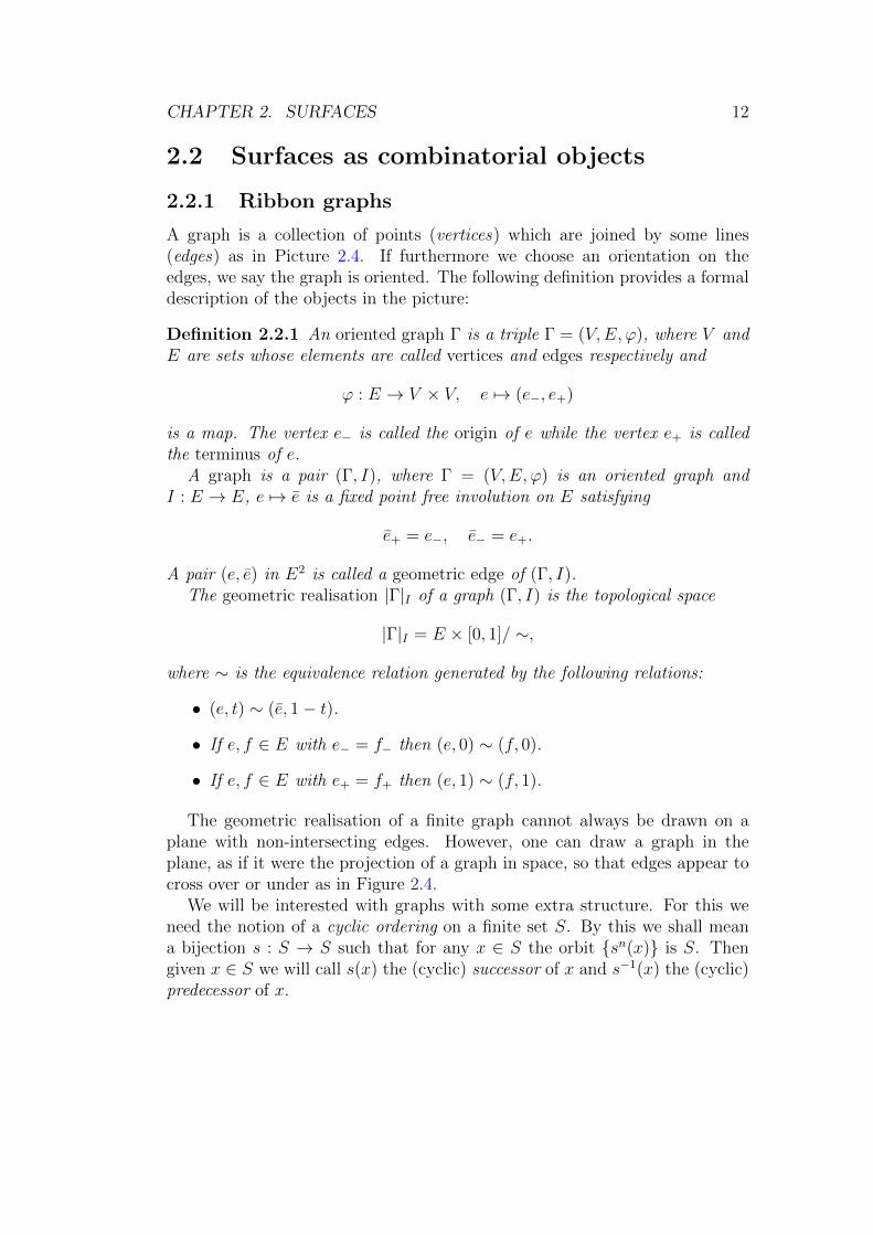
We will be interested with graphs with some extra structure. For this weneed the notion of a cyclic ordering on a finite set S. By this we shall meana bijection s : S → S such that for any x ∈ S the orbit sn(x) is S. Thengiven x ∈ S we will call s(x) the (cyclic) successor of x and s−1(x) the (cyclic)predecessor of x.

CHAPTER 2. SURFACES 13
Figure 2.4: A graph
Definition 2.2.2 [Ribbon graph] Let (Γ, I) be a graph. For v ∈ V , the starof v is
Ev := e ∈ E | e− = v,the set of edges starting from v. A ribbon graph is the data given by a graphand a cyclic ordering on the star of every vertex.
Any planar graph is a ribbon graph. More precisely, given an embedding ofa graph1 into R2 the orientation of R2 induces a cyclic ordering on each of thesets Ev. (We may take a small circle around each vertex intersecting each edgeonly once. Then the circle obtains an orientation from R2 and this defines theordering.
One can always represent a ribbon graph on the plane as the projection ofa graph in space – so again with edges that may cross, over or under – so thatthe cyclic ordering of the edges coincides with the cyclic ordering arising fromthe orientation in the plane as in Figure 2.5.)
Exercise 2.2.3 Show that any embedding of a graph into an oriented surfacegives rise to a cyclic orientation on the sets Ev.
We will now go the other way around and construct surfaces starting fromribbon graphs. As a first step we will embed a ribbon graph into an open (inother words non-compact) oriented surface, even though we remarked a thatit is not always possible to do so in the plane.
1When we talk about an embedding of an graph into a topological space we actually meanan embedding of the geometric realisation of that graph. This slight abuse of language willbe used throughout.
CHAPTER 2. SURFACES 14
Figure 2.5: Cyclic ordering of edges in a planar graph
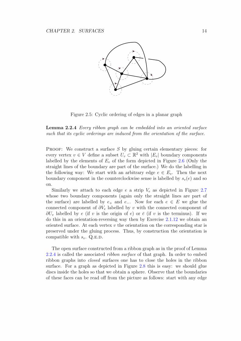
Lemma 2.2.4 Every ribbon graph can be embedded into an oriented surfacesuch that its cyclic orderings are induced from the orientation of the surface.
Proof: We construct a surface S by gluing certain elementary pieces: forevery vertex v ∈ V define a subset Uv ⊂ R2 with |Ev| boundary componentslabelled by the elements of Ev of the form depicted in Figure 2.6 (Only thestraight lines of the boundary are part of the surface.) We do the labelling inthe following way: We start with an arbitrary edge e ∈ Ev. Then the nextboundary component in the counterclockwise sense is labelled by sv(e) and soon.
Similarly we attach to each edge e a strip Ve as depicted in Figure 2.7whose two boundary components (again only the straight lines are part ofthe surface) are labelled by e+ and e−. Now for each e ∈ E we glue theconnected component of ∂Ve labelled by v with the connected component of∂Uv labelled by e (if v is the origin of e) or e (if v is the terminus). If wedo this in an orientation-reversing way then by Exercise 2.1.12 we obtain anoriented surface. At each vertex v the orientation on the corresponding star ispreserved under the gluing process. Thus, by construction the orientation iscompatible with sv. Q.e.d.
The open surface constructed from a ribbon graph as in the proof of Lemma2.2.4 is called the associated ribbon surface of that graph. In order to embedribbon graphs into closed surfaces one has to close the holes in the ribbonsurface. For a graph as depicted in Figure 2.8 this is easy: we should gluediscs inside the holes so that we obtain a sphere. Observe that the boundariesof these faces can be read off from the picture as follows: start with any edge

CHAPTER 2. SURFACES 15
Figure 2.6: A surface associated with a vertex
Figure 2.7: A surface associated with an edge
e and follow this edge to the next vertex. Then take the successor of e andcontinue until you get a closed curve. The curve constructed this way will bethe boundary of a disc in the surface we want to construct.
This procedure works also in more complicated situations as depicted inFigure 2.9 and we formalise it in the following definition:
Definition 2.2.5 Let Γ be a ribbon graph. A face is an equivalence class – upto cyclic permutation – of n-tuples (e1, . . . , en) of edges such that e+
p = e−p+1
and se+p (ep) = ep+1 for all 1 ≤ p ≤ n, where the addition is modulo n.
Note that every oriented edge is contained in a unique face.
Definition 2.2.6 A graph Γ embedded in a surface S is filling if each con-nected component of S \ |Γ| is diffeomorphic to the disc.

CHAPTER 2. SURFACES 16
Figure 2.8: A graph with three faces
Figure 2.9: A graph with one face
CHAPTER 2. SURFACES 17
Then we have:
Proposition 2.2.7 Every ribbon graph Γ has a filling embedding into a com-pact oriented surface S. The connected components of S \ |Γ| are in bijectionwith the faces of Γ.
Proof: The edges of a face define a circle in the ribbon surface. We glue adisc for each of these circles. We thus obtain a closed surface. Q.e.d.
Exercise 2.2.8 What surfaces do you obtain by performing the above con-struction from the ribbon graphs depicted by Figures 2.8 and 2.9 respectively?
The surface obtained from a ribbon graph by Proposition 2.2.7 is in factunique in a very strong sense. To make this precise, we will need the followingbasic fact from point-set topology:
Lemma 2.2.9 [Clutching Lemma] Let X = U ∪V be a decomposition of atopological space X into closed subsets U, V . If f1 : U → Y and f2 : V → Y arecontinuous maps from U and V into some topological space Y with f1|U∩V =f2|U∩V then the induced map f : X → Y is continuous.
Using this we can show the following weak uniqueness result:
Proposition 2.2.10 Let Γ ⊂ S, Γ′ ⊂ S ′ be filling ribbon graphs of compactoriented surfaces and let ϕ : Γ → Γ′ be an isomorphism of ribbon graphs.Then ϕ induces an orientation-preserving homeomorphism ϕ : |Γ| → |Γ′| ofgeometric realisations and this extends to a homeomorphism S → S ′.
Proof: It is easy to see that ϕ extends to the geometric realisation andfurther to the closure of the associated ribbon surfaces. Let
S \ |Γ| =∐f∈F
Df , S ′ \ |Γ′| =∐f∈F
D′f .
Let SΓ and SΓ′ be the ribbon surfaces associated with |Γ|, |Γ′|. Then
S = SΓ ∪(∐f∈F
df
),
where df is a disc slightly smaller than Df and
SΓ ∩(∐f∈F
df
)=∐
∂df

CHAPTER 2. SURFACES 18
is a union of circles. The same statement is true for S ′. By Lemma 2.2.9 itthen suffices to construct for each f ∈ F a homeomorphism df → d′f which
agrees on the boundary ∂df with the extension of ϕ to SΓ . But if ψ : T1 → T1
is any given homeomorphism of circles then there is an obvious way to extendit to the corresponding discs. Indeed, every element x of the disc D may bewritten in polar coordinates as
x = reiθ
for some r ∈ [0, 1] and some eiθ ∈ T1. But then we may simply define ψ(reiθ) :=rϕ(eiθ) to obtain the desired homeomorphism. Q.e.d.
Combining this with Proposition 2.2.7 we obtain:
Corollary 2.2.11 For any ribbon graph Γ there exists a unique compact ori-ented surface SΓ (up to homeomorphism) such that Γ can be embedded as afilling ribbon graph into SΓ.
Corollary 2.2.11 will enable us to classify surfaces up to homeomorphism.A classification up to diffeomorphism is possible along the same lines, but itwould require a stronger form of the corollary. Namely, one would have toprove that any homeomorphism of surfaces is homotopic to a diffeomorphismand thus a ribbon graph determines the surface even up to diffeomorphism.This becomes harder to prove and we will not pursue a classification up todiffeomorphisms here.
Corollary 2.2.11 allows us to construct surfaces starting from ribbon graphs.The following proposition is a converse to this corollary.
Proposition 2.2.12 Every compact oriented surface admits a filling ribbongraph.
We will not prove Proposition 2.2.12 here. The problem of constructinga filling ribbon graph is equivalent to the probably more familiar problem ofconstructing a triangulation of a given surface. Indeed the set of edges ofthe triangulation will yield a filling ribbon graph. There are several standardmethods in order to produce a triangulation (and hence a filling ribbon graph),but any of them uses some basic results from either Riemannian geometry orMorse theory, which we do not want to discuss here.
2.2.2 Classification of surfaces I: Existence
By Corollary 2.2.11 a convenient description of compact surfaces is given bytheir ribbon graphs. We consider a family Γg, g ≥ 1 of ribbon graphs given

CHAPTER 2. SURFACES 19
Γ1
Figure 2.10: The graph Γ1
Γ6
Figure 2.11: The graph Γg for g = 6
as follows: Take g copies of the graph shown in Figure 2.10 and glue themtogether as shown in Figure 2.11 to produce the graph with g petals.
The graph Γ1 has one face and with some imagination one sees that theassociated surface S1 := SΓ1 is a torus. Similarly, each copy of Γ1 in Γggives rise to a torus with a hole and the holes of two consecutive tori areglued together. Thus, after some gymnastics, Sg := SΓg is the surface of ahandlebody with g handles.
There is another description of Sg which turns out to be useful: Let Dg bethe disc in Sg corresponding to the unique face of Γg. Then Sg is obtainedfrom gluing the boundary of Dg. Each (oriented) edge of Γg occurs preciselyonce in the boundary of Dg. More precisely, let ai, bi be the two edges of the

CHAPTER 2. SURFACES 20
Figure 2.12: The surface S3
a
ab b
c
d
c
de
e
Figure 2.13: Constructing S3 by gluing a disc
i-th copy of Γ1 in Γg. Then the boundary of Dg is given by the series of edges
a1, b1, a−11 , b−1
1 , . . . , ag, bg, a−1g , b−1
g .
For g = 3, this is depicted in Figure 2.13.It is convenient to define S0 := S2, the two-sphere. Then we can state
one-half of the classification of surfaces as follows:
Theorem 2.2.13 Every compact oriented surface S is homeomorphic to oneof the surfaces Sg for g ≥ 0.
Proof: Using Proposition 2.2.12, we choose a filling ribbon graph Γ for S.If the graph has no edges, then S must be the two-sphere S2. Thus we mayassume that Γ has at least one edge. We will now deform the graph Γ into agraph Γg without changing its filling property. The theorem will then followfrom Corollary 2.2.11. Suppose firstly, that Γ has more than one face. Then

CHAPTER 2. SURFACES 21
f1
f2
f ′
Figure 2.14: Reducing the number of faces
there exists a geometric edge (e, e) such that e and e are contained in differentfaces. Let Γ′ be the graph obtained from Γ by deleting e and e. Then Γ′ isstill filling for S but has one face less as in Figure 2.14. Iterating this processwe end up with a filling graph with only one face. Thus we may assume thatΓ has only one face.
Secondly, we reduce the number of vertices as in Figure 2.15. Let Γ = (V,E)be a graph embedded in S by the map ϕ. If Γ have more than two vertices,there exists an edge e joining the two different vertices e+ and e−. Let Γ′ =(V ′, E ′, ϕ′) where
• the new set of vertices is obtained by crushing the two vertices e+ ande− to one new vertex e0, V ′ = (V \ e+, e−) ∪ e0,
• the new set of edges is E ′ = E \ e, e
• we define the new embedding ϕ′ by sending the new vertex e0 to a pointin the geometric image of ϕ(e) and extending it to the edges which pre-viously started from e±. Such a construction only requires to work in aneighbourhood of e and can be given a precise model.
Again this reduction of vertices does not change the fact that Γ is filling andreduces the number of vertices by one without increasing the number of faces.Hence we may assume that Γ has only one vertex and one face. This meansthat S is obtained by gluing the boundary of a polygon. The sides of thepolygon are labelled by the edges of Γ and by definition of face every edgeoccurs precisely one. The gluing is finally given by identifying e and e withreversed orientation.
If there are no edges left, then S is the two-sphere S2 and we are done.Thus assume there are still edges left. We will call a pair of geometric edges

CHAPTER 2. SURFACES 22
v1v′
v2
Figure 2.15: Reducing the number of vertices
a
ab
b
Figure 2.16: Linked Edges
((a, a), (b, b)) linked if their relative position is as in Figure 2.16. We claimthat any geometric edge is linked to at least one other geometric edge. Indeed,from the ribbon graph point of view, a geometric edge which is not linked toany other edge would produce an additional face contradicting our assumptionthat there is only one face. Thus we are left to prove the following claim:
Given a linked pair (a, a), (b, b) of geometric edges, there is a way to rear-range the labelling of the polygon without changing the resulting quotient spacesuch that
• a, b, a, b appears as a subsequence,
• and no subsequence of type c, d, c, d is destroyed during this process.
Indeed, if the claim is true then we can relabel the edges of the polygon insuch a way that we obtain one of the graphs Γg.
For the proof of the claim we give an explicit construction which consists ofadding and deleting certain edges of the graph. Such a procedure is depictedin Figure 2.17. The figure has to be read as follows. The main horizontal stepis as follows:
First we add an edge which is dotted in the picture. We therefore obtaintwo faces have different colours in the picture. Then we erase in the graph the

CHAPTER 2. SURFACES 23
green edge, which has the effect on the polygon to glue together these two greenlines in the red one.
Then we repeat this procedure two more times as is depicted in the picture.We observe that no consecutive subsequence of the form c, d, c, d has beendestroyed in this construction. The resulting surface (which is homeomorphicto the one before) is thus brought into a new position such that all edges lie onthe boundary. In the final picture we have created an additional subsequenceof the form a, b, a, b which proves the claim and finishes the proof of thetheorem. Q.e.d.
a
a
a
a
Figure 2.17: Moving linked edges into generic position
2.3 The fundamental group of a surface
2.3.1 The fundamental group of a topological space
The result obtained in Theorem 2.2.13 is not yet a complete classification ofcompact oriented surfaces as we do not know yet whether some of the surfacesSg for distinct g are homeomorphic. In order to show that this does not

CHAPTER 2. SURFACES 24
happens, we need an invariant that distinguishes the surfaces Sg from eachother.
This invariant is the fundamental group– the central object of these seriesof lectures – and we briefly recall its definition:
Definition 2.3.1 Let X, Y be a topological spaces.
(i) A (parametrised) loop in X based at x0 ∈ X is a continuous map γ :[0, 1] → X with γ(0) = γ(1) = x0. Denote by Ω(X, x0) the set of loopsin X based at x0.
(ii) The composition of two based loops γ0, γ1 ∈ Ω(X, x0) is defined to be
(γ0 ∗ γ1)(t) :=
γ0(2t), 0 ≤ t ≤ 1
2
γ1(2t− 1), 12≤ t ≤ 1
(This is continuous by Lemma 2.2.9.)
(iii) Let f0, f1 : Y → X be continuous maps which agree on a subset A ⊂ Y .Then f0 and f1 are called homotopic relative A, denoted f0 ' f1 (rel A),if there exists a map H : [0, 1]× Y → X with
H(0, y) = f0(y),
H(1, y) = f1(y),
∀a ∈ A, H(s, a) = f0(a) = f1(a).
The map H is then called a homotopy relative A. A space X is calledcontractible if id : X → X is homotopic to a constant map X → X, x 7→x0 for some x0 ∈ X.
(iv) Two based loops γ0, γ1 ∈ Ω(X, x0) are called homotopic if they are ho-motopic relative 0, 1. (Notice the abuse of language. If two loops arehomotopic in the sense of (iii) we will call them freely homotopic.) Theset of homotopy classes of loops based at x0 is denoted π1(X, x0).
Exercise 2.3.2 (i) Show that composition descends to a well-defined map∗ : π1(X, x0)× π1(X, x0)→ π1(X, x0).
(ii) Show that with this multiplication (π1(X, x0), ∗) is a group.
Definition 2.3.3 The group (π1(X, x0), ∗) is called the fundamental group ofX at x0.

CHAPTER 2. SURFACES 25
Exercise 2.3.4 Let x0, x1 ∈ X and let γ : [0, 1]→ X with γ(0) = x0, γ(1) =x1. Show that
π1(X, x0)→ π1(X, x1), [α] 7→ [γ ∗ α ∗ γ−]
is an isomorphism, where composition of paths is defined as composition ofloops above and γ−(t) := γ(1− t). Conclude that the isomorphism type of thefundamental group of a arcwise connected space X does not depend on thebase point.
Definition 2.3.5 An arcwise connected space X is called simply-connected ifπ1(X, x0) is trivial for some (and hence any) x0 ∈ X.
In some cases the fundamental group can be computed directly:
Exercise 2.3.6 (i) Show that any contractible space (in particular the disc)is simply-connected.
(ii) Let T be a topological space, S be a subset of T . Let D be the unit discand T1 its boundary. Let finally ϕ : T1 → S be a homeomorphism, showthat there is a surjective group homomorphism π1(T )→ π1(T ∪ϕ D).
(iii) Using (i) and (ii), show that the 2-sphere is simply-connected.
Covering and fundamental group
In general, direct computations of the fundamental group using the above def-inition are rarely possible. Usually the fundamental group of a space is com-puted from a realisation of the space as a nice quotient of a simply-connectedone. For this we introduce the following notions:
Definition 2.3.7 Let Γ be a (discrete) group acting on a space M. Then theaction is called free if it has no fixed point, in other words γ.m = m for someγ ∈ Γ, m ∈ M implies γ = e. The action is proper if for any compact setK ⊂M the set
ΓK := γ ∈ Γ | γK ∩K 6= ∅is finite.2
Then the following is a weak version of the main theorem of covering spacetheory:
2Proper actions make sense for topological groups: we then require that ΓK is compact.Here we use the discrete topology on Γ and in this context one also uses the terminologyproperly discontinuous action in order to emphasize the fact that the group is endowed withthe discrete topology.
CHAPTER 2. SURFACES 26
Theorem 2.3.8 [Covering Theorem] Let M be a locally connected, simplyconnected space M . Let x0 be any point in M . For any, x let γ(x) be a pathfrom x0 to x.
Let Γ be a group acting freely and properly on M and π be the projectionfrom M to Γ\M . Then the map
Γ→ π1(Γ\M,π(x0)), γ 7→ [π(γ(x))],
is a group isomorphism and does not depend on the choices of the paths γ(x).In particular,
π1(Γ\M, [x]) ∼= Γ.
2.3.2 Cayley graph and presentation complex
Using Theorem 2.3.8, there is a way to realise any given group Γ as the funda-mental group of a topological space. More precisely given a group Γ, we shallconstruct a simply-connected space C2(Γ) on which Γ acts freely and properly.Then the theorem implies that π1(Γ\C2(Γ), x) ∼= Γ for any x ∈ Γ\C2(Γ).
For the construction of C2(Γ) we proceed as follows: start with a presenta-tion of Γ of the form
Γ = 〈c1, . . . , ck |R1 = · · · = Rp = e〉,
where R1, · · ·Rp are certain words on c1, . . . , ck. By adding further generatorsand relations if necessary we may assume that there is a fixed point free invo-lution denoted cj 7→ cj for j = 1, . . . , k on the set of generators such that cj isinverse to cj as an element of Γ. Let us call such a presentation admissible.
Definition 2.3.9 Assume that we are given an admissible presentation of thegroup Γ. Then the Cayley graph of Γ with respect to the given presentation isC(Γ) = (V,E), where
• the set of vertices is given by V = Γ
• the vertex η is joined to the vertex γ by an oriented edge (labelled by thegenerator ci) if η = γci.
• the orientation-reversing involution on the set of oriented edges is theinvolution that associates to the edge joining η to γ labelled by ci, theedge from γ to η labelled by c−1
i .
Example 2.3.10 Let F be a free group over a set X. Then F has a presen-tation
F = 〈xx∈X | ∅〉

CHAPTER 2. SURFACES 27
In order to bring this into an admissible presentation, we add one generatorx−1 for each x ∈ X and obtain a new presentation
F = 〈x, x−1x∈X | xx−1 = x−1x = e〉.The vertices of the Cayley graph are labelled by reduced words over the setof generators x, x−1x∈X , where a reduced word is a word in these letterswithout subwords of the form (x, x−1) for x ∈ X. There is a geometric edgelabelled by (x, x−1) for x ∈ X between (x1, . . . , xk) and (x1, . . . , xk, x), wherex1, . . . , xk ∈ X. The corresponding Cayley graph C(F ) is a tree and hence itsgeometric realisation |C(Γ)| is simply-connected.
In general the geometric realisation of a Cayley graph need not be simply-connected. However, it is easy to compute the fundamental group using anadmissible presentation:
Exercise 2.3.11 Let Γ = 〈c1, . . . , ck |R1 = · · · = Rp = e〉 be an admissiblepresentation of a group Γ and let F be the free group on generators c1, . . . , ck.Denote by R the subgroup of F normally generated by the relations R1, . . . , Rp.
(i) Show that F and hence R act freely and properly on the geometricrealisation |C(F )| of the Cayley graph of the free group F with respectto the given presentation.
(ii) Show that |C(Γ)| ∼= |C(F )/R| and conclude that π1(|C(Γ)|) ∼= R.
Let Rj, 1 ≤ j ≤ p be a relation in Γ, written as Rj = ci1 · · · cik where the cjare generators. Then any γ ∈ Γ satisfies
γci1 · · · cik = γ,
thus there exists a loop in C(Γ) starting from γ consisting of edges labelledby ci1 , · · · , cik in precisely that ordering. In the geometric realisation of C(Γ)these form a circle and we can glue a disc along this circle to |C(Γ)| for anysuch loop. The resulting space is called the presentation 2-complex of Γ withrespect to the given presentation and denoted C2(Γ). The case of the groupZ2 with the admissible presentation
〈a, b, a−1b−1 | aba−1b−1 = aa−1 = bb−1 = e〉is depicted in Figure 2.18.
Exercise 2.3.12 Use the special form of π1(C(Γ)) derived in Exercise 2.3.11to prove that the image of π1(|C(Γ)|) in π1(C2(Γ)) is trivial. (Hint: It sufficesto prove that the generators gRig
−1 of π1(|C(Γ)|) are mapped to contractibleloops!) Then apply Exercise 2.3.6 to conclude that C2(Γ) is simply-connected.

CHAPTER 2. SURFACES 28
a a
a a
a ab
b b
b
b
b
Figure 2.18: A presentation 2-complex of Z2
Observe that the action by left multiplication of Γ on itself induces anaction on C(Γ), in other words an action of the set of vertices which preservesadjacency. This in turn induces an action of Γ on the geometric realisation|C(Γ)|. This action extends to C2(Γ). Indeed, the action of Γ maps eachloop to another loop and the corresponding homeomorphism of circles in thegeometric realisation extend to the discs bounded by these circles as in theproof of Proposition 2.2.10.
Proposition 2.3.13 The action of Γ on C2(Γ) is free and proper. Thus
π1(Γ\C2(Γ)) ∼= Γ.
Exercise 2.3.14 Prove Proposition 2.3.13.
2.3.3 Classification of surfaces II: Uniqueness
We apply Proposition 2.3.13 to prove the following uniqueness part of theclassification:
Theorem 2.3.15 The fundamental group of the surface Sg is given by
π1(Sg) ∼= 〈a1, b1, . . . , ag, bg |g∏i=1
aibia−1i b−1
i = e〉.
These groups are non-isomorphic for different choices of g.
CHAPTER 2. SURFACES 29
Proof: For g = 0 the theorem predicts π1(S2) = e which was proved inExercise 2.3.6. Thus let us assume g ≥ 1 and abbreviate
Ag := 〈a1, b1, . . . , ag, bg |g∏i=1
aibia−1i b−1
i = e〉.
Adding the inverse of the generators this presentation, we construct the as-sociated Cayley graph and presentation 2-complex. Then Γ\C2(Γ) is homeo-morphic to gluing a disc whose boundary is labelled by a1, b1, a
−11 , b−1
1 , . . . , b−1g
according to this labelling. We have seen before that this is a description of Sgand thus the identity π1(Sg) = Ag follows from Proposition 2.3.13. The laststatement of the theorem follows from the fact that
Hom(Ag,R) ∼= R2g.
Q.e.d.
A group isomorphic to Ag := π1(Sg) will be called a surface group. By The-orem 2.2.13 and Theorem 2.3.15 we can associate to every compact orientedsurface a unique non-negative integer g in such a way that π1(S) ∼= Ag. Thisinteger is the genus of S. Using this terminology, we summarise the classifi-cation by saying that any compact oriented surface is uniquely determined byits genus and conversely every non-negative integer occurs as the genus of asurface.
2.4 Combinatorial versions of the fundamen-
tal group
We shall need other versions of the fundamental group: First we will explainhow to compute the fundamental group of the surface out of a filling ribbongraph. Secondly we will explain how to build the fundamental group usingcovers and coverings.
2.4.1 A combinatorial description using a ribbon graph
In this section, we relate the filling ribbon graph of a surface and its funda-mental group. For the first part of the classification we have used the existenceof filling ribbon graphs. These ribbon graphs are not unique but they can bedeformed into a filling ribbon graph of type Γg. Using different ribbon graphsone can compute the fundamental group of the surface in different ways. Thisgives rise to different presentations of surface groups.

CHAPTER 2. SURFACES 30
Let Γ be a ribbon graph. Denote by E, V and F respectively the set of itsedges, vertices and faces.
Definition 2.4.1 [Combinatorial loops and paths] A discrete path isa finite sequence (e1, . . . , En) so that e+
i = e−i+1. The starting point of such apath is e−1 , its end point is e+
n . A path is a discrete loop if its end and startingpoints coincide. A loop is based at the vertex v0 if v0 is its starting point. Theinverse path of e = (e1, . . . , en) is e := (en, . . . , e1)
We may now define the ribbon fundamental group. Let F (E) be the freegroup generated by the edges; observe that every path defines an element ofF (E). Let Lv0
Γ be the image of the loops based at v0 in F (E). Observe thatLv0 is a subgroup of F (E). Let Rv0
Γ be the subgroup of Lv0Γ normally generated
by faces f = (e1, . . . , ek).
Definition 2.4.2 [Ribbon fundamental group]
• The group Lv0Γ is the group of loops based at v0.
• The group Rv0Γ is the group of homotopically trivial loops.
• The ribbon fundamental group is
π1(Γ, v0) = Lv0Γ /R
v0Γ .
• Two path e and f with the same starting and end points are homotopicif the loop e.f belongs to the group of homotopically trivial loops.
Observe that if Γ′ is a subgraph of Γ we have a natural surjection from π1(Γ, v0)to π1(Γ, v0). Moreover if Γ is a filling graph embedded in a surface S, we havea natural map i from π1(Γ, v0) to π1(S, v0) which is build by sending everycombinatorial loop to its geometric realisation.
Theorem 2.4.3 Let S be a surface and Γ a filling ribbon graph in S. Thenatural map i described in the previous definition is an isomorphism from theribbon fundamental group to the fundamental group of the surface.
The proof is essentially the same as for Theorem 2.3.15. We leave the detailsto the reader.
CHAPTER 2. SURFACES 31
2.4.2 A combinatorial description of the fundamentalgroup using covers
The fundamental group of a cover
We want to define fundamental groups through covers. Recall that a opencover of X is a family of open sets whose reunion is X. Since we shall onlyconsider open covers, we will usually omit the word open when we speak ofopen cover.
Definition 2.4.4 [Path] Let U = Ui∈I be a cover of a space X. A path onthe cover based at i0 is an element i0 . . . ip of the free group FI generated by Isuch that Uij ∩Uij+1
= ∅. A loop is a path (i0, . . . , ip) so that i0 = ip. A trivialloop is a loop of the form (j0, . . . jp, I, J,K, jp, . . . j0) where UI ∩ UJ ∩ Uk 6= ∅.Definition 2.4.5 [Fundamental group] Let U = Ui∈I be a cover of M .The fundamental group πU1 (M) of the cover is the group of loops based at i0– considered as a subgroup of the free group generated by I – up to the groupgenerated by trivial loops.
In other words, the fundamental group of a cover U = Ui∈I is the fun-damental group of the 2-complex, whose set of vertices is the set I, set ofedges is the set of intersecting open sets, and set of faces is the set of triplesof intersecting open sets.
We observe that if V = Vjj∈J is a refinement of U , that is a cover suchthere exists a map f : J → I so that Vj ⊂ Uf(j), then we have a natural map
f : πV1 (S)→ πU1 (S).
Exercise 2.4.6 Show that the map above does not depend on the choice ofthe map f . Show that the map above is surjective provided the open sets Uiare connected.
We shall admit the following result which relies on Van Kampen Theorem[Hat02].
Theorem 2.4.7 Let Ui be a cover such that the Ui are simply connectedand Ui ∩ Uj are connected. For every i, let xi be an element of Ui. For everypair (Ui, Uj) of intersecting open sets, we choose a path γij joining xi to xj.We associate to every loop on the covering i0 . . . in where in = i0, the loopγi0i1 ? . . . γin−1in. This construction is an isomorphism from πU1 (M) to π1(M) .
It follows from this result that if X admits a cover by simply connected setswith connected intersections, then we have a well defined surjective map fromπ1(M) to πU1 (M) for any cover U of X.
Exercise 2.4.8 Reprove Theorem 2.4.3 using Theorem 2.4.7.

CHAPTER 2. SURFACES 32
Covers and covering maps
A Galois cover of group G is a map π : Σ→ S, where G acts properly withoutfixed points on Σ, S = Γ\Σ and π the projection. A trivialising cover is acover U = Uii∈I of S so that for every i,
π−1(Ui) =⊔γ∈G
γVi.
We can relate covers and coverings as follows. Let π : Σ → S be a Galoiscover of group G. Let U be a trivialising cover of S as above so that every Uiis connected. Let finally U = gVii∈I,g∈G.
Proposition 2.4.9 Let π : Σ → S be a Galois cover. Let U be a trivialisingcover of S for π, so that the intersection of two open sets is connected. Then,we have a short exact sequence
0→ πU1 (Σ)→ πU1 (S)→ G.
Proof: The hypothesis on U = Uii∈I yields that we can lift uniquely everypath U -path to a U -path, which maps trivial loops to trivial loops. Hence weobtain the short exact sequence
0→ πU1 (Σ)→ πU1 (S)→ G.
Q.e.d.
2.5 Cohomology of Surfaces
This whole section is a warm up for the next chapter. We shall give – andprove – more general statements in this next chapter. However, we specialisein this section to the standard situation of – untwisted – cohomology groupsso that the reader can parallel this construction with the more general one.
2.5.1 De Rham cohomology
In this section we shall introduce and compute the cohomology groups of asurface S. These groups have several constructions, in this section we shalluse the existence of a differentiable structure on S and construction the deRham cohomology groups using differential forms.
Let us be a little more general and let M be smooth manifold of dimensionn.

CHAPTER 2. SURFACES 33
Derivative, tangent and cotangent spaces
Let m be a point on M . Let C00(M,m) be the vector space of functions that
vanishes at m.We say two functions f and g of C0
0(M,m) have the same derivative at mif we can write
f − g =i=n∑i=1
ϕiψi,
where ψi and ϕi belong to C00(M,m). We observe that, when M = Rn, f and
g have the same derivative at m if and only if df(m) = dg(m). Then,
• the cotangent space T∗mM is set of equivalent classes of the relation“having the same derivative” of functions of C0
0(M,m).
• The derivative df(m) of a function f is the class of the function f−f(m)in T∗mM ,
• Finally the tangent space TmM is the dual to T∗mM . Elements of T∗Mare called tangent vectors at m.
Recall that smooth functions on a manifolds are functions which are smoothin any charts and we denote by C∞(M) the vector space of smooth maps onM . A map F from a manifold M to another manifold N is smooth, if for anyg ∈ C∞(N), f F is smooth, thus giving rise to a linear map from C∞(N) toC∞(M).
Clearly such a smooth map F defines a linear map from T∗f(m)N to T∗mMand thus a linear map, called the tangent map TmF , from TmM to Tf(m)N .
Differential forms
Informally speaking, a differential k-form – or shortly a k-form – is a mapwhich assigns to each point m ∈ M a vector ωm ∈
∧k T∗mM for some k ≥ 0,such that furthermore ωm varies “smoothly” (see below).
Example 2.5.1 1. By convention,∧0 T∗mM := R and thus a (smooth)
0-form is just a (smooth) function.
2. If f is a smooth function on M then its differential dxf is a linear formon tangent space and thus df is a 1-form.
If U is a contractible open coordinate chart with coordinates x1, . . . , xn thenthe differentials dxj generate the algebra of differential forms. This means that

CHAPTER 2. SURFACES 34
any k-form on U can be written as
ω|U =∑
I=(i1,...,ik)
ωIdxi1 ∧ · · · ∧ dxik
with ωI : U → R. The functions ωI are the coefficients of ω in the chart.We say that a k-form ω is smooth, if for every point m ∈ M there exists a
coordinate chart around m for which the coefficients of ω are smooth. In thatcase, one checks easily that the coefficients of ω are smooth in any chart.
We will only consider smooth forms and thus we reserve both the termsdifferential form and k-form for smooth k-forms.
We denote by Ωk(M) the vector space of k-forms on M . Note that Ωk(M) =0 for k > dimM . By convention, we set Ωk(M) = 0 for k < 0. The wedgeproduct defines maps Ωk(M)× Ωl(M) into Ωk+l(M). Thus
Ω•(M) :=⊕k∈Z
Ωk(M)
is a Z-graded C∞(M)-algebra.
Support, pullbacks
The support of a differential form ω is the closure of those points x for whichthere exist a chart such that at least one coefficient of ω does not vanish at x.A form ω is compactly supported, if its support is a compact subset of M . Wedenote by Ωk
c (M) the vector space of compactly supported k-forms on M .Let M1 and M2 be manifolds and F : M1 → M2 be a smooth map, the
associated pullback map
F ∗ : Ω•(M2)→ Ω•(M1)
is defined as follows: Let ω ∈ Ωk(M2), let m be any point in M , let X1, . . . , Xk
be tangent vectors at m, then
F ∗ωm(X1, . . . , Xk) := ωF (m)(TmF (X1), . . . ,TmF (Xk)).
Integration
Differential forms can be integrated on oriented manifolds. Let us consider thecase of an open subset U of Rn. Let ω = fdx1 ∧ · · · ∧ dxn ∈ Ωn(U) be withcompact support. Then we define∫
U
ω :=
∫U
fdx1 ∧ · · · ∧ dxn :=
∫U
f dλn(x1, . . . , xn),

CHAPTER 2. SURFACES 35
where λn is the n-dimensional Lebesgue measure.If ϕ is any diffeomorphism then∫
U
ϕ∗ω = ±∫ϕ(U)
ω,
where the sign is positive if ϕ preserves orientation and negative if ϕ reversesthe orientation. As a consequence of this sign irritation we can only defineintegration for oriented manifolds:
Proposition 2.5.2 If M is an oriented n-dimensional manifold then thereexists a unique linear map
Ωnc (M)→ R, ω →
∫M
ω
such that if ω is supported in a chart (U, x) with x orientation-preserving then∫M
ω =
∫x(U)
(x−1)∗ω.
Convention 2.5.3 Suppose N ⊂M is a k-dimensional oriented submanifoldand ι : N → M denotes the inclusion. Then we can integrate any k-formω ∈ Ωk(M) over N . We will use a slight abuse of notation and denote this by∫
N
ω :=
∫N
ι∗ω.
Exterior derivatives
The following proposition is a crucial step in defining cohomology.
Proposition 2.5.4 There exists a unique family of linear operators
dk : Ωk(M)→ Ωk+1(M),
with the following properties:
(i) d0 coincides with the usual differential C∞(M)→ Ω1(M).
(ii) dk(fdk−1α) = d0f ∧ dk−1α for f ∈ C∞(M), α ∈ Ωk−1(M).
The proof relies on a simple recursion that we shall not reproduce here: thekey fact is that locally any k-form is a sum of expressions of the form fdk−1α.
Note that (ii) immediately implies
dkdk−1 ≡ 0.
This allows the following definition.

CHAPTER 2. SURFACES 36
Definition 2.5.5 A k-form ω ∈ Ωk(M) is closed if dkω = 0 and exact if thereexists α ∈ Ωk−1 with ω = dk−1α.
Then define the k-th de Rham cohomology group of M is
HkdR(M) := ker dk/Im dk−1.
In other words the quotient of the space of closed forms by the set of exactforms. The dimension
βk := dimHkdR(M)
is called the k-th Betti number of M .
More generally, recall that a complex of vector spaces or modules is a familyC• of vector spaces Ck together with linear maps dk from Ck → Ck+1 so thatdk+1 dk = 0. Thus, using this language, the differential forms on a manifoldtogether with the differential form form a complex called the de Rham complex
De Rham cohomology has strong links with homotopy:
Lemma 2.5.6 [Poincare Lemma] If U is a contractible manifold, then ev-ery closed form is exact. In other words, Hk
dR(U) = 0 for all k > 0.
The Poincare Lemma is a corollary of the fundamental
Lemma 2.5.7 [Homotopy Lemma] Let M be a manifold and F0 and F1 betwo smooth homotopic maps from M to N . Let β be a closed form in N . Thenthe form
F ∗0 β − F ∗1 β,is exact.
If one has a covering of a space by contractible submanifolds (which alwaysexists for manifolds) then one can use Poincare’s Lemma in order to reduce thecomputation of Hk
dR(M) to a combinatorial counting process. This is calledthe Mayer-Vietoris argument and will be discussed and applied below.
The relation between the de Rham differential of a manifold and integrationis described by the following generalisation of the fundamental theorem ofcalculus:
Theorem 2.5.8 [Stokes formula]Let M be an oriented manifold with boundary ∂M . Then∫
∂M
ω =
∫M
dω.
In particular, if ∂M = ∅ then the integral of a differential form only dependson its cohomology class.

CHAPTER 2. SURFACES 37
Hurewicz Theorem
We can now the first de Rham cohomology group with the fundamental groupas follows.
Theorem 2.5.9 [Hurewicz Theorem] Let M be a connected manifold. Leth be the mapping defined by
H1(M,R) → Hom(π1(M),R),[ω] 7→ h[ω],
where for every curve γ : T1 →M
h[ω](γ) =
∫T1
γ∗ω.
Then, h is an isomorphism.
Exercise 2.5.10 Use Stokes Formula and the Homotopy Lemma to show thatthe above statement actually makes sense. Then prove Hurewicz Theorem.
Thus we have the identification.
H1dR(M,R) ∼= Hom(π1(M),R).
Observe that since R is abelian,
Hom(π1(M),R) ∼= Rep(π1(M),R).
Thus the first de Rham cohomology group of a manifold is our first exampleof a representation variety. Moreover, and this will be important for us in thesequel, we can identify H1
dR(M,R) with the tangent space of the representationvariety. We will see later on, that in the case of a general representationvariety, the tangent spaces (at the smooth points) can still be identified with atwisted version of de Rham cohomology. Thus, the de Rham cohomology willappear as a toy version of the more general constructions that we are going todevelop.
Extension of differential forms
We close this paragraph with an auxiliary result on extending differentialforms:
Lemma 2.5.11 [Extension Lemma] Let M be a manifold, V, U open sub-sets of M with V ⊂ U . If ω = dα on U for some α ∈ Ωk(U) then there existsα ∈ Ωk(M) such that ω|V = dα|V .
The proof uses the existence of a smooth bump function with support in Uwhich is 1 on V and 0 outside U and is left to the reader.

CHAPTER 2. SURFACES 38
2.5.2 Ribbon graphs and cohomology
When S is a compact orientable connected surface, we will describe and com-pute in a combinatorial way the cohomology using ribbon graphs rather thandifferential forms.
To explain this approach, let S be a surface and let Γ be a filling ribbongraph for S. As S is uniquely determined by Γ, the de Rham cohomologyof S is also uniquely determined by Γ. We are now going to give an explicitcomputation of the cohomology of S using Γ.
We will consider a generalisation of this method in great detail later onwhen we discuss twisted cohomology. Therefore we only explain the basicconstructions here and do not provide any proofs. The reader is invited tospecialise the more general proofs given in Section 4.1.7 below to the presentcase.
Denote by V,E, F the sets the vertices, edges and faces of the filling ribbongraph Γ. We define the sets of combinatorial 0-cochains, 1-cochains and 2-cochains of Γ by
C0Γ(S) := f : V → R,
C1Γ(S) := f : E → R | f(e) = −f(e),
C2Γ(S) := f : F → R.
We then define differentials
d0 : C0Γ(S) → C1
Γ(S), (d0f)(e) := f(e+)− f(e−),
d1 : C1Γ(S) → C2
Γ(S), (d1α)(f) :=∑e∈f
α(e).
Then d1 d0 = 0 because given a face f every vertex occurs as often as theorigin of an edge of f as it occurs as a terminus of such an edge. It is convenientto define Ck
Γ(S) := 0 for k 6∈ 0, 1, 2 and dk : CkΓ(S)→ Ck+1
Γ (S) as the zeromap for k 6∈ 0, 1. Then dk+1dk ≡ 0 for all k ∈ Z and thus we may define:
Definition 2.5.12 The group
HkΓ(S) :=
ker dk
Im dk−1
is called the k-th cohomology group of S with respect to Γ.
Note that by definition, dimHkΓ(S) <∞.

CHAPTER 2. SURFACES 39
We now relate the cohomology groups of Γ to the de Rham cohomologygroups of M : We define maps ιk : Ωk(S)→ Ck(Γ) by
ι0 : Ω0(S)→ C0Γ(S), ι0(f)(v) := f(v);
ι1 : Ω1(S)→ C1Γ(S), ι1(α)(e) :=
∫e
α;
ι2 : Ω2(S)→ C2Γ(S), ι0(ω)(f) :=
∫f
ω.
We set ιk ≡ 0 for k 6∈ 0, 1, 2. Here we have abused notation and identified avertex, edge or face with its image in the geometric realisation of Γ, consideredas a subset of S. For α ∈ Ωk(S) we will write α := ιk(α). Observe:
Proposition 2.5.13 For any α ∈ Ωk(S),
dα = dα.
In particular, ιk(Zk(M)) ⊂ ker dk, ιk(B
k(M)) ⊂ Im dk and thus ιk induces amap
ιk : HkdR(M)→ Hk
Γ(S).
Exercise 2.5.14 Derive 2.5.13 from Stokes Formula.
In fact one has:
Theorem 2.5.15 The maps ιk : HkdR(S) → Hk
Γ(S) defined by Proposition2.5.13 are isomorphisms.
Theorem 2.5.15 has a number of consequences. An obvious one is the fol-lowing:
Corollary 2.5.16 (i) The (de Rham) cohomology groups of a compact ori-entable surface are finite-dimensional.
(ii) The groups HkΓ(S) do not depend on the choice of filling Ribbon graph
which is used in order to define them.
For a manifold with finite-dimensional cohomology spaces we define theEuler characteristic as the alternating sum of its Betti numbers, in other words
χ(M) :=dimM∑i=0
(−1)iβi.
Let us compute the Euler characteristic for compact orientable surfaces. Forthis we use the following easy algebraic fact:

CHAPTER 2. SURFACES 40
Lemma 2.5.17 Let 0 → C0 d0
−→ . . .dn−1
−−−→ Cn → 0 be a finite complex offinite-dimensional vector spaces Ck, in other words dk+1dk = 0. Let
Hk :=ker dk
Im dk−1
be the associated cohomology groups. Thenn∑k=0
(−1)k dimHk =n∑k=0
(−1)k dimCk
We apply this in order to compute the Euler characteristic of a closed sur-face:
Corollary 2.5.18 If S ∼= Sg is a compact orientable surface of genus g thenits Euler characteristic is given by χ(S) = 2 − 2g. In particular, a compactoriented connected surface is uniquely determined up to homeomorphisms byits Euler characteristic.
Proof: If Γ is a filling ribbon graph with vertices V , edges E and faces Fthen
dimC0Γ(S) = |V |, dimC1
Γ(S) =1
2|E|, dimC2
Γ(S) = |F |.Thus Lemma 2.5.17 implies
χ(S) = dimH0Γ(S)− dimH1
Γ(S) + dimH2Γ(S) = |V | − 1
2|E|+ |F |.
If we take for Γ the graph Γg then
|V | = |F | = 1,1
2|E| = 2g,
and the result follows. Q.e.d.
From this we can finally compute the cohomology of a compact orientedsurface:
Corollary 2.5.19 If S ∼= Sg is a surface of genus g then
H0dR(S) ∼= R, H1
dR(S) ∼= R2g, H2dR(S) ∼= R.
Proof: A function with trivial derivative on a connected manifold is constantand therefore
H0dR(S) = Z0
dR(S) = f ∈ C∞(S) | d0f = 0 ∼= R.
The result for H1dR(S) follows from the Hurewicz theorem and our computation
of the surface group . Then χ(S) = 2− 2g forces H2dR(S) ∼= R. Q.e.d.

CHAPTER 2. SURFACES 41
Γ1Γ2
Figure 2.19: Gluing Graphs
Application: gluing ribbon graphs
We had to perform some intellectual gymnastics in order to identify the surfacefilled by a ribbon graph. It is much more easy by now: we just have to computeits Euler characteristic. Exercise 2.2.8 is now much easier to solve. Here is anexercise as an application
Exercise 2.5.20 Let Γ1 be a ribbon graph filling a surface of genus g1. LetΓ2 be a ribbon graph filling a surface of genus g2. Let Γ3 be the ribbon graphobtained in the following way: Draw a circle such that Γ1 and Γ3 are in thetwo distinct connected components of the complement. Then join this circleto Γ1 and Γ2 as in Picture 2.19. Prove that Γ3 fills a surface of genus g1 + g2.
2.5.3 The intersection form
In the next two subsections we will deal with symplectic structures on vectorspaces. Recall the following basic definition:
Definition 2.5.21 Let V be a vector space. A bilinear map V × V → R iscalled a linear symplectic form if it is alternating and non-degenerate.
In this subsection, we construct a symplectic form on H1dR(S). As explained
before, we view this cohomology group as the tangent space of the representa-tion variety Rep(π1(S),R) at a base point. Therefore constructing a symplecticform on H1
dR(S) is the same as constructing a fibrewise symplectic form on thetangent space of Rep(π1(S),R). We will later on generalise this procedure tomore general (and in particular, non-abelian) coefficient groups. Again the

CHAPTER 2. SURFACES 42
Figure 2.20: A dual graph
proofs will be given later on in the more general setting of Section 4.1. Herewe will only explain the ingredients for the proof of the following theorem:
Theorem 2.5.22 Let S be a surface. Then the map
i : H1dR(S)×H1
dR(S)→ R, ([α], [β]) 7→∫S
α ∧ β
is a symplectic form.
The map i is called the intersection form of S and it gives a duality onH1dR(S) . It is clear from the definition that i is alternating and bilinear. It is
less clear, whether i is non-degenerate. To prove non-degeneracy we will useonce again ribbon graphs and Theorem 2.5.15. Thus let S be a surface withfilling ribbon graph Γ, and let Γ∗ be its dual. The latter is again a ribbongraph and it is defined as follows: Denote by VΓ, EΓ, FΓ the vertices, edges andfaces of Γ. We define VΓ∗ := FΓ, EΓ∗ := EΓ. If (e, e) is a geometric edge inΓ then e is contained in a unique face f ∈ FΓ = VΓ∗ and e is contained in aunique face f ∈ VΓ∗ . We then define
ϕ∗ : EΓ∗ → VΓ∗ × VΓ∗ , ϕ∗(e) := (f, f).
Then (VΓ∗ , EΓ∗ , ϕ∗) is a directed graph and the involution e↔ e turns Γ∗ into
a graph. Geometrically Γ∗ is obtained by drawing edges between adjoint facesas in Figure 2.20.
Exercise 2.5.23 Show that FΓ∗ and EΓ are in canonical bijection.

CHAPTER 2. SURFACES 43
Definition 2.5.24 Denote by CkΓ, Ck
Γ∗ the combinatorial cochains of Γ and Γ∗
respectively. Then the dual pairing
〈·|·〉 : CkΓ × C2−k
Γ∗ → R
is defined by
〈α | β〉 :=∑
v∈VΓ=FΓ∗
α(v)β(v) (α ∈ C0Γ, β ∈ C2
Γ∗);
〈α | β〉 :=∑
e∈EΓ=EΓ∗
α(e)β(e) (α ∈ C1Γ, β ∈ C1
Γ∗);
〈α | β〉 :=∑
f∈FΓ=VΓ∗
α(f)β(f) (α ∈ C2Γ, β ∈ C0
Γ∗)
and 〈·|·〉 ≡ 0 for k 6∈ 0, 1, 2.
Proposition 2.5.25 (i) The dual pairing 〈·|·〉 : CkΓ × C2−k
Γ∗ → R satisfies
〈dα | β〉 = 〈α | dβ〉 (α ∈ CkΓ, β ∈ C1−k
Γ∗ ).
(ii) The dual pairing descends to a pairing
〈·|·〉 : HkΓ ×H2−k
Γ∗ → R.
(iii) The dual pairing is non-degenerate on HkΓ ×H2−k
Γ∗ for k ∈ 0, 1, 2.
Recall the definition of the map ι1 : Ω1(S)→ C1Γ from the last section. As
EΓ = EΓ∗ and the involution on EΓ and EΓ∗ agree we have C1Γ∼= C1
Γ∗ andthus we have also an isomorphism ι∗1 : Ω1(S) → C1
Γ∗ . We can use these mapsto relate the intersection form on Ω1(S) to the dual pairing. More precisely,we have the following result, which together with Proposition 2.5.25 impliesTheorem 2.5.22:
Lemma 2.5.26 Let α, β ∈ Ω1(S). Then∫S
α ∧ β = 〈ι1(α) | ι∗1(β)〉.
We prove later on a more general result that contains this lemma as a specialcase.
CHAPTER 2. SURFACES 44
2.6 Comments, references and further read-
ings
Instead of using simplicial description of surfaces, we use the approach byribbon graphs – which are also called fat graphs. This approach has the disad-vantage that it is not straightforwardly generalisable, but on the other hand itis perfectly suited for surfaces. Ribbon graphs gain their mathematical popu-larity through the work of Penner [Pen92] who introduced a cell decompositionof Riemann moduli space, which was later used in Kontsevich’s proof of WittenConjecture [Kon92].
The argument proving the classification of surfaces written in these notesis found in Springer [Spr57] which is still a very nice introduction to Riemannsurfaces. Other possible references are Massey, “A basic course in algebraictopology” [Mas91], Stillwell, “Geometry of surfaces” [Sti92].
We presented several aspects of the fundamental groups: first the generaldefinition, then a combinatorial description through ribbon graphs, then finallythrough covers and coverings. These presentations are somewhat ad hoc forsurfaces but we hope that these various points of views will help the readersee different aspects of a fundamental group: as an abstract group, as definedwith generators and relations, as describing coverings and associated to covers.
We chose to present the relation between combinatorial and de Rham co-homology only in the case of surfaces – remark here that the ribbon graph co-homology is slightly different from simplicial cohomology since a ribbon graphdecomposition is not a triangulation. Even though this is a very pedestrianapproach, we hope that it may help the reader go through the general proofs.The classical Bott-Tu [BT82] is an excellent introduction to de Rham coho-mology and its link with combinatorial versions. Even though the categoricaland axiomatic approach to these isomorphisms are more powerful, we findimportant for future use to explain how one can realise these isomorphismsexplicitly.
The book by Hatcher [Hat02] is a remarkable introduction to algebraictopology and fundamental groups which should be used as the basic referencefor fundamental groups and simplicial homology.

Chapter 3
Vector bundles and connections
In this chapter, we introduce the main objects of our study: vector bundles,connections and representation variety. We give two different point of viewson vector bundles, first as a “continuous family” of vector spaces indexed by atopological space, then as cocycles which are of a more combinatorial nature.This allows us in particular to define G-structures on vector bundle. Afterhaving motivating connections by the need to have explicit isomorphisms –depending on choices – between fibres of a vector bundle, we give severaldescription of flat connections using the various languages we have used inparallel for the fundamental group and cohomology: differential geometry,ribbon graphs and coverings.
This allows us to define and give four different models of the representationvariety
Hom(π1(S), G)/G.
3.1 Vector bundles
This subsection is one more time intended to provide a very brief crash courseon the concepts which we shall need. We start with the notion of a vectorbundle.
3.1.1 Definitions
Informally, a vector bundle is a continuous family of vector spaces indexed bya topological space. The following definition makes this precise.
A vector bundle is a triple (L, π,M), where L and M are topological spacescalled the total space and the total space respectively and π : L → M is acontinuous map satisfying the following two conditions:
45

CHAPTER 3. VECTOR BUNDLES AND CONNECTIONS 46
(i) For all m ∈ M the fibre Lm := π−1(m) is a finite dimensional vectorspace isomorphic to a given vector space L.
(ii) For all m ∈M there exists a neighbourhood Um of m and a homeomor-phisms
ϕ : π−1(Um)→ Um × L,which restricts to a linear isomorphism ϕ : Lm′ → m′ × L for anym′ ∈ Um.
The dimension of L is called the rank of the vector bundle and denoted rkL.If rkL = 1, then L is called a line bundle. An open subset satisfying property(ii) is called trivialising. By abuse of language we will simply call L a vectorbundle (over M). A section of (L, π,M) is a continuous map σ : M → L suchthat σ(m) ∈ Lm. We denote by Γ(L) the space of sections of (L, π,M). LetL and L′ be vector bundles over respectively M and M ′. Let ϕ : M → M ′.Then a morphism over ϕ is a fibre-preserving fibrewise linear map ψ : L → L′.In other words the diagram
L → L′↓ ↓M
ϕ−→ M ′
commutes and ψ : Lm → L′m is linear. An automorphism is a morphism overthe identity which is fibrewise invertible. The group of automorphisms of L iscalled the gauge group and denoted G(L).
A more general definition of vector bundles would allow the vector spaceL to jump from one connected component of B to the other. We will mostlybe interested in connected base spaces and therefore we have no need forsuch a general definition here. An advantage of our definition is the factthat isomorphism classes of vector bundles in our sense can be described in auniform way.
A combinatorial interpretation through cocycles
We need an other definition which allows performing constructions and com-putations in a combinatorial way.
Definition 3.1.1 let M be a topological space.
1. A cocycle over M with values in the automorphism groups of a vec-tor space L is a pair (U ,G), where U is an open covering of M andgUV U,V ∈U is a collection of continuous maps gUV : U ∩ V → GL(L)subject to the cocycle condition
gUV gVW = gUW .

CHAPTER 3. VECTOR BUNDLES AND CONNECTIONS 47
2. Two cocycles (U ,G), (U ,G ′) with the same open covering are called di-rectly equivalent if there exists a family of maps hU : U → GL(L) suchthat
g′UV = hUgUV h−1V .
3. A cocycle (U ,G) is called a refinement of the cocycle (U0,G0) if thereexists a map i : U → U0 such that
U ⊂ i(U),
and for all U, V in UgUV = gi(U)i(V )
∣∣U∩V .
4. Two cocycles will be called equivalent if they have directly equivalent re-finements .
We claim that vector bundles over a topological space M up to isomorphismare in one-to-one correspondence with cocycles up to equivalence. Let us ex-plain how the correspondence is obtained: given a cocycle (U ,G), the cocyclecondition ensures that we obtain an equivalence relation ∼ on the space∐
U∈U
U × U × L
by(U, x, v) ∼ (V, x, gUV (x).v).
Then
L :=
(∐U∈U
U × U × L)/ ∼
is the total space of a vector bundle over M , where the projection is given by
π : L →M, [(U, x, v)] 7→ x.
In other words the projection comes from the natural projection on the firstfactors of the direct unions:
L =
(∐U∈U
U × U × L)/ ∼−→
(∐U∈U
U × U)/ ∼= M
Conversely, given a vector bundle (L, π,M) we may choose a trivialisingcovering Uii∈I and trivialisations
ϕi : π−1(Ui)→ Ui × L.

CHAPTER 3. VECTOR BUNDLES AND CONNECTIONS 48
Then we can trivialise the bundle over Ui ∩ Uj in two different ways, namelyvia
ϕij : π−1(Ui ∩ Uj) → π−1(Ui)ϕi−→ Ui × L
orϕji : π−1(Ui ∩ Uj) → π−1(Uj)
ϕj−→ Uj × L.Both ϕij and ϕji are fibre-preserving fibrewise linear homeomorphisms onto(Ui ∩ Uj)× L and we can define the cocycle gij by
ϕji ϕ−1ij : (Ui ∩ Uj)× L→ (Ui ∩ Uj)× L, (m, v) 7→ (m, gij(m)v).
Exercise 3.1.2 Show that the constructions described above indeed give riseto a correspondence between isomorphism classes of vector bundles over Mand equivalence classes of cocycles.
Example 3.1.3 1. For any topological spaceM , the product bundle of rankn is M × Rn → M . A bundle is trivial if it is isomorphic to a productbundle.
2. Vector bundles may be trivial or non-trivial. The Mobius strip (seeFigure 2.1) is a non-trivial line bundle.
3. If M is a manifold, then the tangent bundle TM and the cotangent bundleT∗M are vector bundles.
4. As an exercise, the reader is invited to prove that every vector bundleover the interval is trivial.
3.1.2 Constructions
Algebraic constructions
All algebraic operations that can be performed with vector spaces can beperformed with vector bundles. As an example, we consider direct sums: letL, F be vector bundles over a topological space M . Informally speaking, thebundle L ⊕ F is the bundle with fibre (L ⊕ F)m ∼= Lm ⊕ Fm. We formalisethis idea using cocycles: over some open covering Uii∈I the bundles arerepresented by cocycles gij and hij respectively. Then we define a bundleL ⊕ F with via the block-matrix cocycle
gij ⊕ hij :=
(gij 0
0 hij
).
Similarly, we may construct L ⊗ F ,∧k L, Hom(L,F), L∗ and so on.

CHAPTER 3. VECTOR BUNDLES AND CONNECTIONS 49
Pullback bundle
This important construction can be described informally as follows. Let π :L → M be a bundle over M . Let f : N → M be a continuous map whereN is any topological space. The pullback bundle f ∗(L) is the bundle over Mwhose fibre at m is Lf(m). Again, the notion of cocycle makes this construc-tion precise: assume L → M is defined by the cocycle (Uii∈I , giji,j∈I),then the pullback bundle of L via f is the bundle defined by the cocycle(f−1(Ui)i∈I , gij fi,j∈I). Alternatively, we can describe the total spaceof the pullback bundle as
f ∗(L) := (e, n) ∈ L ×N |π(e) = f(n)
where the projection is given by the projection to the second factor.The following fact will be important for us, although we will not prove it
here. This is a generalisation of the fact that a vector bundle over the intervalis trivial.
Proposition 3.1.4 Suppose that f0, f1 : N → M are homotopic maps andthat L is a vector bundle over M . Then f ∗0 (L) is isomorphic to f ∗1 (L). Inparticular, any vector bundle over a contractible space is trivial.
When N and M are compact, the proof of this proposition is a fairlystraightforward generalisation of the triviality of any vector bundle over theinterval.
Sections along a curve
We will often need to perform operations along a curve in M . A convenientway to express such operations is given by the following definition:
Definition 3.1.5 Let γ : [0, 1] → M be a curve and L → M be a vectorbundle over M . A section along the curve γ is a map v : [0, 1] → L withπ(v(t)) = γ(t). Equivalently, v ∈ Γ(γ∗L).
3.2 Vector bundles with structures
So far we have considered cocycles with values in GL(L), where L is a vectorspace. These cocycles preserve the linear structure of the vector space L.However, we might also want to preserve some additional structure on L likean inner product or a symplectic form or some other tensor. This amounts torestricting the range of our cocycles. We formalise this as follows:

CHAPTER 3. VECTOR BUNDLES AND CONNECTIONS 50
Let G be a topological group and ρ : G → GL(L) a continuous injectivehomomorphism – in other words a faithful linear a representation of G. Weshall in the sequel abusively identify G with its image ρ(G).
Definition 3.2.1 [G-structure] A G-atlas of the vector bundle L over Mis an open cover Ui of M together with a trivialisation of L|Ui as Ui × L sothat the changes of trivialisations are maps with values in ρ(G). Two G-atlasesare equivalent if their union is still a G-atlas. Finally a G-structure is a classof G-atlases up to the equivalence above.
Remark 3.2.2 1. In terms of cocycles, we obtain G-structures from G-valued cocycles which are cocycles (Uii∈I , giji,j∈I), so that gij arewith values in G.
2. We also observe that a G-structure defines for every m in M a subgroupGm of GL(Lm) isomorphic – although not canonically – to G. Moregenerally, a G-structure defines for every m and n a subset Gm,n ofHom(Lm,Ln) equipped with a right transitive action of Gn and a lefttransitive action of Gm, so that Gm,p = Gm,n.Gn,p and Gm,m = Gm.e.
3. The notion of G-structure is also called reduction of the structure groupto G.
We need to extend the previous definitions
Definition 3.2.3 [G-Morphisms] Let L → M and F → N two vector bun-dles with G-structures.
• A G-morphism is a vector bundle map Φ from L to F over a map ϕfrom M to N which is an isomorphism on each fibre and such that thepull back of any G-atlas of F is a G-atlas of L.
• A G-isomorphism is a G-morphism over the identity; with the previousnotation, this means that M = N and ϕ = Id.
• A G-trivialisation is a G-isomorphism with the trivial G-bundle.
• A G-automorphism is a G-isomorphism of a G-bundle with itself.
Definition 3.2.4 [Gauge group] The gauge group G(L) of the G-bundleL is the group of G-automorphisms of the bundle. The gauge group naturallyidentifies with the group of sections σ : M → End(L), so that for every m,σ(m) belongs to Gm.

CHAPTER 3. VECTOR BUNDLES AND CONNECTIONS 51
If L = M × L is a trivial bundle with the trivial G-structure, then G(L) =C0(M,G).
Example 3.2.5 Let B be a bilinear form on a vector space L. Denote bySO(L,B) the group of linear automorphisms of L that preserve B. Then aSO(L,B)-structure on a vector bundle L is the same as a continuously varyingfamilies of tensors of the same type as B in each fibre. Indeed, given v, w ∈ Lmwe can compute B(v, w) in a trivialisation, and, as the coordinate changes areorthogonal with respect to B, this quantity is independent of the trivialisationchosen.
Tensor field
The following definition and proposition will be used several times in the sequel.
Definition 3.2.6 [Tensor Field] Let L1, . . . ,Ln and F be vector bundlesover the same space M . A map
A : Γ(L1)× . . .× Γ(Ln)→ Γ(F)
is a tensor field if there exists a section a of Hom(L1⊗Ln,F) so that for everypoint m in M
A(σ1, . . . , σn)m = am(σ1m, . . . , σ
nm).
Observe that every tensor field A is a morphism of C0(M)-algebras, that isfor every function f1, . . . fn on M and sections σi of Li we have
A(f1σ1, . . . , fnσn) = f1 . . . fnA(σ1, . . . , σn).
Conversely, the following proposition will be helpful:
Proposition 3.2.7 Every morphism of C0(M)-algebras
A : Γ(L1)× . . .× Γ(Ln)→ Γ(F)
is a tensor field.
In the sequel, we shall also abusively use the term tensor field either for thesection of Hom(L1 ⊗ Ln,F) or the map from Γ(L1)× . . .× Γ(Ln) to Γ(F)
Proof: We only sketch the proof. We first observe the following immediateresult: if A is a map from C0(M) to itself which is a morphism of C0(M)-algebras, then there exists a function g so that A(f) = gf . More generally,if L and V are vector spaces and A is a map from C0(M,L) to C0(M,V )

CHAPTER 3. VECTOR BUNDLES AND CONNECTIONS 52
which is a morphism of C0(M)-algebras, then there exists an element a ofC0(M,Hom(L, V )) so that (A(f))(m) = a(m)
(f(m)
). In other words, the
proposition above is true for trivial bundles.Let us move to the general case using the notation of the proposition. We
observe that if fi, gi are sections of Li equal on some neighbourhood U of mthen
A(f1, . . . , fn)m = A(g1, . . . , gn)m
Indeed, let ϕ be a function equal to 1 at m and with support in U , then
A(f1, . . . , fn)m = A(ϕ.f1, . . . , ϕ.fn)m = A(ϕ.g1, . . . , ϕ.gn)m = A(g1, . . . , gn)m
After this observation is made, we are reduced to a local situation. Sincea vector bundle is locally trivial, a straightforward extension of the initialargument of this proof yields the proposition. Q.e.d.
3.2.1 Vector bundles over manifolds
All we have said so far applies to topological spaces, topological groups and con-tinuous maps. The definitions naturally extend to “smooth spaces”, “smoothgroups” and “smooth maps”. By “smooth spaces”, we mean manifold; by“smooth group”, we mean a Lie group, that is group which is also a manifoldin such a way that group multiplication and inversion are smooth maps – asour first (and only examples) we shall only consider classical groups such asSLn(R), SU(n) etc. A vector bundle is a smooth vector bundle if the definingcocycles can be taken to be smooth. Smooth sections make a natural sense,and we also observe that pullbacks of smooth bundles via smooth maps aresmooth. Similarly, algebraic constructions preserves smooth bundles. In thefollowing, we will almost exclusively deal with smooth bundles. Therefore wewill make the following conventions:
Convention 3.2.8 All vector bundles, cocycles, G-structures, . . . are smoothunless otherwise mentioned and we denote by Γ(L) the smooth sections of thesmooth vector bundle L.
For manifolds there are some bundles which are of particular importance.In the first place these are the tangent bundle TM and the cotangent bundleT∗M := (TM)∗. Via the algebraic constructions described in Section 3.1.2we can construct new bundles out of these bundles. We have encountered thebundles ∧
kT∗M (k ≥ 0)

CHAPTER 3. VECTOR BUNDLES AND CONNECTIONS 53
and using our new notation
Ωk(M) = Γ(∧
kT∗M).
In other words a section of∧
kT∗M is nothing but a k-form on M .More generally, if L is a vector bundle over M , we denote by Ωk(M,L)
the vector space of differential k-forms with values in L, that is the space ofsections of the tensor bundle
∧k(T∗M)⊗L. By convention,∧0(T∗M)⊗L = L,
so that Ω0(M,L) = Γ(L).Finally, we have an easy extension of our previous result about tensor fields:
Proposition 3.2.9 Let L1, . . . ,Ln and F be (smooth) vector bundles over thesame manifold M . Every morphism of C∞(M)-algebras
A : Γ(L1)× . . .× Γ(Ln)→ Γ(F)
is a (smooth) tensor field.
3.3 Connections
Let us start with an informal explanation of what is a connection: if π : L →Mis a vector bundle and m,m′ two points in M then the fibres Lm and Lm′are isomorphic. However, there is no way in general to construct a naturalisomorphism between different fibres for one very good reason: not all vectorbundles are trivial.
We can nevertheless remark that any vector bundle over the interval istrivial, and, in particular the restriction of the vector bundle to any pathjoining m to m′ can be trivialised, albeit non canonically. Informally speaking,a connection is a “coherent” way to trivialise the vector bundle over any path.
Les us be a little more precise in order to justify the next paragraph. Aconnection will be a procedure with associates to any path γ : [0, 1]→M fromm to m′ an isomorphism
Hol(γ) : Lm → Lm′ ,
called the holonomy of γ. Such a procedure will be realised by any path in Mto a path in L. More precisely, given a curve γ : [0, 1] → M and a startingpoint v0 ∈ Lγ(0) a connection will construct for us a section v(t) along γ withv(0) = v0. Then the holonomy of γ is the map which maps the startingpoint v0 to the endpoint v(1) of v. Here is one example: if M = Rn andL = TRn = Rn × Rn, the natural lift of γ : [0, 1] → Rn and (γ(0), v) ∈ L

CHAPTER 3. VECTOR BUNDLES AND CONNECTIONS 54
is a constant lift v(t) = (γ(t), v). This constant lift is uniquely determinedby the property that its derivative in the direction of the path γ vanishes.Thus in order to define a connection we need to define a “constant section”along a curve; and, in order to define a constant section, we need to define a“derivation” along a curve. This is the idea underlying the next definition.
3.3.1 Koszul connection
Definition 3.3.1 [Koszul connection] A (Koszul) connection on the vec-tor bundle L over M is a linear map
∇ :
Γ(L) → Ω1(M,L),
σ 7→ (X 7→ ∇Xσ).
such that for all smooth function f on M , we have the Leibniz rule
∇X(fσ) = df(X) · σ + f∇X .
Observe that by definition ∇fXσ = f∇X(σ).Alternatively, we can think of a Koszul connection as a bilinear map from
Γ(TM)×Γ(L) to Γ(L) which associates to a vector field X on M and a sectionσ of L, a new section ∇Xσ of L such that for all functions f in C∞(M)
∇Xfσ = f∇X(σ) + df(X).σ,
∇fXσ = f∇X(σ).
Here is the relation between the two definitions: according to the first def-inition, we may plug a tangent vector X ∈ TmM and a section σ of L in aconnection in order to obtain an element ∇Xσ of Lm. But we might as welltake a vector field X ∈ Γ(TM) and a section σ of L in order to produce asection s of L according to the rule
sm := ∇X(m)σ.
We will use the abbreviation∇Xσ := s
for this construction. Hence, by definition,
(∇Xσ)(m) := ∇X(m)σ.
The starting example of a Koszul connection is the following one:

CHAPTER 3. VECTOR BUNDLES AND CONNECTIONS 55
Example 3.3.2 Let L = M × L be a trivial bundle, where L is a vectorspace. In particular, Γ(M ×L) ∼= C∞(M,L). In this case, we have a preferredconnection of L call the trivial connection and denoted by D. This trivialconnection is given by
DX(σ) = Dσ(X).
In particular, we see that every trivial bundle admits a connection. Moregenerally,
Proposition 3.3.3 Every vector bundle admits a connection.
Proof: If f1, . . . , fn are functions on M such that∑fi = 1 and ∇i are
connections on M then∇ =
∑i
fi∇i
is also a connection. This formula and remarks also makes sense if each ∇i
is only defined on the restriction of the vector bundle over the support of fi.Thus, we may take a trivialising cover for L over M , a corresponding smoothpartition of unity and combine trivial connections on the trivialising open setsusing the partition of unity. Q.e.d.
There will be many connections on a given vector bundle L and the followingproposition shows that the space of connections is an affine space.
Proposition 3.3.4 If ∇1,∇2 are connections on L then there exists a tensorfield A ∈ Ω1(M,End(L)) such
∇1Xσ −∇2
Xσ = Am(X)σ,
that for all m ∈M , X ∈ TmM , σ ∈ Γ(L).Conversely, given a connection ∇ and a tensor A ∈ Ω1(M,End(L)), ∇+A
is a connection. In particular, the connections on L form an affine spacemodelled on Ω1(M,End(L)).
This proposition follows from Proposition 3.2.9 and the fact – easily checkedfrom the definition – that
(X, σ)→ ∇1Xσ −∇2
Xσ
is a morphism of C∞(M)-algebras.
CHAPTER 3. VECTOR BUNDLES AND CONNECTIONS 56
3.3.2 Constructions
The constructions (algebraic operations and pullbacks) that we performedabove for vector bundles generalise to bundles with connection. We explainsome of these constructions here and leave the remaining constructions to thereader.
1. Suppose ∇L and ∇F are connections on bundles L and F over the samemanifold M . Then there is a connection ∇ = ∇L ⊗∇F on L⊗F whichfor X ∈ TmM and a product section σ = σL ⊗ σF of L ⊗ F is given by
∇Xσ := ∇LXσL ⊗ σF(m) + σL(m)⊗∇FXσF .
2. If ∇ is a connection on L then there is a unique connection ∇∗ on thedual bundle L∗ such that for all X ∈ Γ(TM), v ∈ Γ(L) and w ∈ Γ(L∗),
X〈v |w〉 = 〈∇Xv |w〉+ 〈v | ∇∗Xw〉,where 〈· | ·〉 : Γ(L) × Γ(L∗) → C∞(M) denotes the dual pairing and Xacts as a differential operator on the smooth function 〈v |w〉.
3. If ∇ is a connection on a bundle L over M and f : N →M is a smoothmap between manifolds then there is a unique connection , called thepullback connection and denoted f ∗∇, on f ∗L satisfying
(f ∗∇)X(f ∗σ) = f ∗(∇Tf(X)σ), (3.1)
for all σ ∈ Γ(L) and X ∈ TN .
All these constructions are performed by the following two steps: first consid-ering the situation in the trivial case, then using cocycles. For instance let usexplain the construction for the pullback connection. If L is trivialised over Uas U ×L, then we can write ∇ = D+A, then we define f ∗∇ over V := f−1(U)as D + f ∗A. Then, f ∗∇ is the unique connection over V satisfying Condition(3.1), thus by uniqueness we see that the definition of f ∗∇ coincides over in-tersection of trivialising open sets – with possibly different trivialisations. Itfollows that we can define coherently f ∗∇ over M .
3.3.3 Gauge equivalence and action of the gauge group
The definition of pullback enables us to to define an action of the on the spaceof connections. Indeed, if f is an automorphisms of L and ∇ is a connectionon L, then f ∗(∇) is also a connection on L.
Two connections ∇1 and ∇2 are said to be gauge equivalent if there exists anelement f of the gauge group – that is an automorphism of the vector bundle– so that ∇1 = f ∗(∇2). In other words, gauge equivalence classes are orbits ofthe gauge group.
CHAPTER 3. VECTOR BUNDLES AND CONNECTIONS 57
3.3.4 Holonomy along a path
We have motivated the introduction of connections by considering the problemof lifting a curve. Now let us see that the formal machinery introduced in thelast subsection solves the curve lifting problem:
Definition 3.3.5 [Differentiation along a curve] Let L be a vectorbundle over M and let ∇ be a connection on L. Let v(t) be section along acurve γ : [0, 1] → M . Then the derivative of v(t) along γ(t) is the sectionalong γ(t) given by
∇γv := (γ∗∇)∂tv,
where ∂t is the fundamental vector field of the curve γ and v is regarded as asection of γ∗(L).
Definition 3.3.6 [Parallel section along a curve] Let L be a vectorbundle over M and let ∇ be a connection on L. A section v(t) along a curveγ : [0, 1]→M is called ∇-parallel along γ if
∇γv = 0.
Now we can prove that a connection indeed lifts paths:
Proposition 3.3.7 Let π : L → M be a vector bundle with connection ∇.Let γ : [0, 1]→ M a curve and v0 ∈ Lγ(0). Then there exists a unique parallelsection v = vv0 along γ such that v(0) = v0. Thus ∇ defines a linear map
Hol∇(γ) :
Lγ(0) → Lγ(1)
v0 7→ vv0(1).
Proof: As [0, 1] is contractible, the bundle γ∗L is trivial. We fix a trivialisa-tion and identify γ∗L ∼= [0, 1] × L. By Proposition 3.3.4 the connection γ∗∇takes the form γ∗∇ = D + A under this identification, where D denotes thetrivial connection and A is some tensor. Then v ∈ Γ(L) is parallel if and onlyif
v = B · v,where B = −A(∂t). Thus lifting γ with initial point v0 = (γ(0), v0) is the sameas solving the ordinary differential equation
v = B · v,
with initial condition v(0) = v0. The proposition then follows from the exis-tence and uniqueness theorem for ordinary differential equations. Q.e.d.

CHAPTER 3. VECTOR BUNDLES AND CONNECTIONS 58
Definition 3.3.8 [Holonomy along a path] The map Hol∇(γ) from Lγ(0)
to Lγ(1) is called the holonomy of ∇ along γ.
Example 3.3.9 [Holonomy of the trivial connection] Let L = M×Lbe the trivial product vector bundle over M with fibre L. As usual denote byD the trivial connection on L. let γ : [0, 1] → M be a path. Let finallyγv ∈ Γ(γ∗L) be the constant section given by γv(t) := (γ(t), v).
Our initial observation is that γv is D-parallel along γ. Hence γv is theparallel lift of γ with initial value v. It follows that
HolD(γ)(γ(0), v) = γv(1) = (γ(1), v).
Thus identifying each fibre x×L with L via (x, v)→ v, we see that HolD(γ)induces the identity between the two copies of L sitting over γ(0) and γ(1).
It is easy to see that the connection can be reconstructed from the asso-ciated holonomy maps; moreover parallel sections can be described using theholonomy. We leave this as an exercise:
Exercise 3.3.10 Let ∇,∇′ be connections on a vector bundle L → M . Sup-pose that for all γ : [0, 1]→M the maps Hol∇(γ) and Hol∇
′(γ) coincide. Show
that ∇ = ∇′.
Exercise 3.3.11 Let σ be a section of L. Then σ is parallel if and only if forevery path γ from x to y, we have σ(y) = Hol∇(γ) · σ(x).
3.3.5 Holonomy and linear differential equations
Parallel sections and holonomies have interpretations using differential equa-tions. We summarise this in the following proposition whose proof is left tothe reader.
Proposition 3.3.12 Let γ : [a, b]→ M be a path. We choose a trivialisationof L along γ as [a, b]×L0 so that ∇ = D +A where D is the trivial connectionand A ∈ Ω1([a, b],End(L0)). Let B = A(∂t). A section σ along γ is nowinterpreted as a map X : [a, b]→ L0. Then σ is parallel along γ if and only ifX satisfies
(∗) d
dtX(t) = B(t)X(t).
In particular the holonomy from γ(u) to γ(s) along γ is the resolvent of thisequation.
CHAPTER 3. VECTOR BUNDLES AND CONNECTIONS 59
3.3.6 Curvature
One should notice that a connection does not produce just one canonical iso-morphism between different fibres, but rather one isomorphism for each curveγ in M joining the two base points. Different curves may lead to differentholonomy maps. We, however, will mainly be interested in connections whoseholonomy depends only on the homotopy class (relative endpoints) of a curve.In order to characterise these connections we introduce the following notion:
Definition 3.3.13 Let ∇ be a connection on a vector bundle π : L → M .Then the curvature of ∇ is
R∇ : TM × TM → End(L)
which is given by
R∇(X, Y )σ := ∇X∇Y σ −∇Y∇Xσ −∇[X,Y ]σ,
for vector fields X, Y ∈ Γ(TM) and a section σ ∈ Γ(L).The connection is called flat if and only if R∇ vanishes identically.
Exercise 3.3.14 Show that R∇ defines a tensor field R∇ ∈ Ω2(M,End(L)).
Example 3.3.15 (i) If D is the trivial connection of L = M × L thenRD = 0 by Clairaut (or Schwarz) Theorem (or the symmetry of thesecond derivatives) and thus D is flat.
(ii) Suppose L = M × R is the trivial line bundle over M . Then any con-nection on L is of the form ∇α = D + α, where α is a 1-form on Mand
R∇α
= dα.
Thus D + α is flat if and only if α is closed.
3.3.7 Flat connections
The curvature will measure whether the holonomy is invariant under homo-topies. The next theorem is fundamental and we shall only prove the easy partof it (see comments section for textbook references).
Theorem 3.3.16 Let ∇ be a connection on a vector bundle π : L →M . Thenthe following are equivalent:
(i) ∇ is flat, in other words R∇ ≡ 0.

CHAPTER 3. VECTOR BUNDLES AND CONNECTIONS 60
(ii) If γ, γ′ : [0, 1]→M are homotopic with fixed extremities then
Hol∇(γ) = Hol∇(γ′).
(iii) The bundle L admits a trivialisation over every simply-connected opensubset of M in which ∇ is trivial.
Notice in contrast to (iii) that not every bundle on a simply connected spaceis trivial: the famous case is the 2-sphere and its tangent space; one can notcomb a sphere [Mil97].
Proof: The obvious implication is (iii)⇒ (i), which follows from the fact thatthe trivial connection is flat. Let us show that (ii) implies (iii): given a simply-connected open subset U of M fix a point x0 ∈ U and join any point x ∈ U withx0 via a path γx contained in U . Then the map Hol(x) := Hol∇(γx) : Lx → Lx0
depends only on x but not on the choice of γx because any two paths in Ujoining x and x0 are homotopic relative endpoints (even in U). Then the map
i : L|U → U × Lx0 , v 7→ (π(v),Hol(π(v))(v)
is a trivialisation with trivial holonomy and thus ∇ is trivial on U by Exercise3.3.10. Finally, the hard part of the proof is to show that (i) ⇒ (ii). For thiswe refer to the literature quoted in the Section 3.6. Q.e.d.
Note that there is also an easy direct argument for the implication (iii)⇒ (ii). Namely, the holonomy of the trivial connection does not depend ona chosen path. A special case of the last theorem is given by the followingcorollary:
Corollary 3.3.17 Let ∇ be a flat connection on a vector bundle π : L → Mand x0 ∈M . Then, the map
π1(M,x0)→ GL(Lx0), [γ] 7→ Hol∇(γ),
is a group homomorphism called the holonomy homomorphism of ∇.
3.3.8 Connections preserving structures
What is a connection in the world of G-structures? When the bundle isequipped with a G-structure, it makes sense to speak of a connection pre-serving the G-structure. Let G be a subgroup of GL(L) which is a smoothsubmanifold. Recall the Lie algebra g of G is the tangent space to G at theorigin which we consider as a vector subspace of End(L).
CHAPTER 3. VECTOR BUNDLES AND CONNECTIONS 61
Definition 3.3.18 Let M be a manifold and L → M be a vector bundleequipped with a G-structure. A connection ∇ on L is a G-connection if, forany open set U , for any G-trivialisation over U , there exists a 1-form ω on Uwith values in g such that in that trivialisation
∇|U = D + ω,
where D is the trivial connection.
Example 3.3.19 Suppose G = SO(B). Then a G-structure is the same as afibrewise tensor of the same type as B, and a G-connection is a connection forwhich this family of tensors is parallel.
The following is a straightforward verification:
Proposition 3.3.20 Let ∇ be a G-connection on a vector bundle π : L →Mand x0 ∈M .
(i) Then the curvature of ∇ is given by
R∇ = Ω,
where 2-form Ω ∈ Ω2(M, g).
(ii) If ∇ is flat then the holonomy homomorphism is Gx0-valued.
(iii) Finally, if flat two connections are gauge equivalent, then the associatedholonomy homomorphisms are conjugate by an element of Gx0.
3.3.9 The holonomy map of a flat connection
The previous proposition associates to every flat connection a conjugacy classof homomorphism in G since Gx0 is isomorphic up to conjugation with G. Thisleads to the following definition.
Definition 3.3.21 [Holonomy representation of a flat connection]Let ∇ be a flat G-connection. Then the holonomy representation of ∇ is theconjugacy class of the representation of π1(M) in G described in Proposition3.3.20.
The following proposition is crucial.
Proposition 3.3.22 Two gauge equivalent flat connections yield conjugateholonomy representations. Conversely, if two flat connections have the sameholonomy they are conjugate.

CHAPTER 3. VECTOR BUNDLES AND CONNECTIONS 62
Proof: The first part of the proposition is obvious using the last statementin Proposition 3.3.20. Let us concentrate on the second part. We will produceeffectively the gauge equivalence: let ∇1 and ∇2 be two connections with thesame holonomy representation. Let us fix a base point x0. Then we choose forevery x in M a path cx from x0 to x. We finally define
gx = (Hol∇1
(cx))−1 Hol∇
2
(cx).
Since ∇1 and ∇2 are flat, gx only depends on the homotopy class of cx. Sincemoreover the two connections have the same holonomy, the reader is requiredto check tha gx is independent on the choice of the homotopy class. It followsthat for every path joining γ two points x and y,
g−1y Hol∇
1
(γ)gx = Hol∇2
(γ).
Let finally g : x → gx be the associated element of the gauge group. Then,by the previous equation, the holonomy of every path is the same for g∗∇1
and ∇2. Then by Exercise 3.3.10 g∗∇1 = ∇2 and thus ∇1 and ∇2 are gaugeequivalent. Q.e.d.
3.4 Combinatorial versions of connections
We define in this section two combinatorial analogues of connections and flatconnections together with the associated gauge equivalences. The two nextparagraphs mirror the combinatorial constructions of the fundamental groupin Section 2.4. In the next section, we will show all these notions are equivalent.
3.4.1 Discrete connections on ribbon graphs
We now explain what is a connection in the world of ribbon graphs. Let Γ bea ribbon graph whose set of edges is E, set of vertices is V and set of faces isF .
Definition 3.4.1 [Discrete G- connections] A discrete G-connection onΓ is a map
∇ : E → G, e 7→ ge,
satisfying ge = g−1e . We will write ∇ = gee∈E.
Definition 3.4.2 [Discrete gauge equivalence] Denote by (GE)′ ⊂ GE
the set of discrete connections. The group GV is called the gauge group of ΓThe gauge group acts on the space of connections via
gvv∈V .hee∈E := ge+hege−e∈E.Two discrete connections in the same GV -orbit are called gauge equivalent.

CHAPTER 3. VECTOR BUNDLES AND CONNECTIONS 63
Recall that a sequence of edges (e1, . . . , en) is a path on Γ if (ej)+ = (ej+1)−for j = 1, . . . , n− 1. Denote by P the space of paths in Γ.
Definition 3.4.3 [Paths and holonomy] Let ∇ = gee∈E be a discreteconnection. The holonomy of ∇ is the map
Hol(∇) : P → G, (e1, . . . , en) 7→ ge1 · · · gen .
Faces are special paths:
Definition 3.4.4 [Flat connections] The curvature of ∇ is the map
R∇ := Hol(f)f∈F ∈ GF .
A discrete connection is called flat if R∇ = Id.
We then have the discrete analogue of Theorem 3.3.16
Proposition 3.4.5 Let ∇ be a discrete flat connection on a ribbon graph. Lete and f be two homotopic paths with the same endpoints. then
Hol∇(e) = Hol∇(f).
The proof of the proposition relies on the following observation: homotopicallytrivial loops have trivial holonomy. Let S be the surface associated to a ribbongraph. The previous proposition and the description of π1(S) using ribbongraphs 2.4.3 yields the following definition.
Definition 3.4.6 [Holonomy representation] Let Γ be a ribbon graphfilling a surface S. The holonomy map gives rises to the holonomy homomor-phism of the discrete G-connection from π1(S) to G, which associates to everydiscrete closed path its holonomy.
Remark: Two gauge equivalent discrete connections give rise to conjugateholonomy representations.
3.4.2 Local systems
We now define discrete G-connections in the context of covers of surfaces inthe same spirit that we defined fundamental groups using covers of a surface.
If U = Uii∈I is a covering, let
I(n) := (i1, . . . , in) ∈ In | gi1 ∩ . . . gin 6= ∅.

CHAPTER 3. VECTOR BUNDLES AND CONNECTIONS 64
Definition 3.4.7 [G-Local systems] Let M be a manifold and let U =Uii∈I be a covering. Given a group G, a G-local system over M on U is acollection of elements (gij)(i,j)∈I(2) of elements of G such that moreover
gijgjk = gik,
whenever (i, j, k) ∈ I(3). Observe that every local system on U gives rise to alocal system on any refinement of U .
The gauge group of the covering U is the group GI . The gauge group actson the space of local systems over U by
(hi)i∈I : (gij) 7→ higijh−1j .
Two G-local systems on the same covering U are called gauge equivalent aslocal systems if they lie in the same orbit of the gauge group.
Two G-local systems are equivalent as local systems if they are in they aregauge equivalent on some common refinement.
Remark: If G is abelian, then in the language of Cech cohomology a G-localsystem is just a Cech-1-cocycle and an equivalence class of such systems is justthe corresponding cohomology class. Then standard arguments in cohomologyshow that the set of equivalence classes of G-local systems are naturally identi-fied with H1(M,G). Therefore one should think of the collection of equivalenceclasses of G-local systems as a non-abelian version of H1(M,G).
We defined in Section 2.4.2 fundamental groups using covers. We extendour previous construction now:
Definition 3.4.8 [Holonomy of a G-local system] The holonomy ofthe path (i0, . . . , ip) for the G-local system (gij) is the element gi0,i1 . . . gin−1,in
of G. By definition of a local system, the holonomy of a trivial loop is trivial.The holonomy representation is the map from πU1 (M) to G which associatesto each path its holonomy.
One more time two gauge equivalent local systems yield conjugate repre-sentations; we leave this check to the reader.
3.5 Four models of the representation variety
In this paragraph, we gather the information that we have collected on smoothand discrete connections, local systems and representations of the fundamentalgroup of the surface. All these objects will be identified in this section up tosome equivalence. Let us be more precise: we have four collections of objectsto which we associated “holonomy” representations, namely

CHAPTER 3. VECTOR BUNDLES AND CONNECTIONS 65
(1) Pairs (L,∇), where L is a G-vector bundle over the surface S and ∇ isa flat G-connection on L, up to gauge equivalence.
(2) Equivalence classes of discrete flat G-connections with respect to a fillingribbon graph Γ, again up to gauge equivalence.
(3) Equivalence classes of G-local systems on S on a given covering.
(4) Homomorphisms of π1(S) into G up to conjugation.
These four collections of objects give rise to different models for the repre-sentation variety, each of which will turn out to be useful at some stage. Theequivalence of the descriptions (1), (3) and (4) holds for general manifolds andwe shall prove them in this generality.
Remark again that when G = R, the above equivalences are the well-knownisomorphisms between de Rham, simplicial and Cech cohomology as well asHurewicz Theorem
We shall denote by Mi with i ∈ 1, 2, 3, 4 the corresponding set of equiv-alence classes in the four cases under consideration.
We shall also denote by Rep(π1(S), G) = M4 the space Hom(π1(S), G)/Gwhere G acts on Hom(π1(S), G) by conjugation.
3.5.1 Flat connections and local systems
We need a definition.
Definition 3.5.1 [Good covering] An open covering Uii∈I of a manifoldM is called a good covering if it satisfies the following condition. For all n ∈ Nand all i1, . . . , in ∈ I the subset
Ui1,...,in := Ui1 ∩ · · · ∩ Uin
is empty or contractible.
Any manifold admits a good covering, but we will not prove this here sincethis is more easily achieved using Riemannian geometry. Anyhow, we aremainly interested in the case of surfaces and in this case one can constructgood coverings associated to ribbon graphs.
Theorem 3.5.2 Let M be a manifold. Then there exists a one-to-one corre-spondence preserving the holonomy between gauge equivalence classes of G-localsystems on a good covering and flat G-connections.

CHAPTER 3. VECTOR BUNDLES AND CONNECTIONS 66
Proof: Let (gij) be a G-local system for the good covering Uii∈I of M . Weview gij as a constant map Ui∩Uj → G ⊂ End(L). Then gij defines a cocycle,hence a vector bundle over M , which we call L. By construction we havetrivialisations L|Ui ∼= Ui × L such that the transition maps are the constantfunctions gij. On Ui×V we have the trivial connection Di and thus we obtain aconnection ∇i on L|Ui via pullback. Since the gij are constant linear maps andthe derivative of a constant map with respect to the trivial connection is thelinear map itself we see that ∇i and ∇j coincide on L|Ui,j . Thus there existsa unique connection ∇ on L such that ∇|Ui = ∇i. Thus we have produceda bundle L with connection ∇ from a G-local system. Conversely, given abundle with connection we conclude from Theorem 3.3.16 that it trivialisesover each of the sets Ui and that the connection is the pullback of a trivialconnection. Then the coordinate changes preserve the connection and thus arelocally constant, hence constant. It is easy to check that this gives rise to thecorrespondence claimed in the proposition. Q.e.d.
3.5.2 Local systems and representations
Theorem 3.5.3 Let M be a manifold and G be a Lie group. Then the holon-omy map from the space of flat G-local systems on a good covering – up togauge equivalence – to Rep(π1(M), G) is a bijection.
Equivalently, using the previous correspondence
Theorem 3.5.4 Let M be a manifold and G be a Lie group. Then the holon-omy map from the space of flat G-connections up to gauge equivalence toRep(π1(M), G) is a bijection.
If G is abelian then this correspondence identifies the first cohomology groupH1(M,G) with Hom(π1(M), G). In this case, the correspondence is just theHurewicz Theorem 2.5.9.
Proof: Let us first remark that the universal covering M → M defines aπ1(M) local system.
Indeed, let U = Uii∈I be a good covering. Observe that if π : M → M isthe universal cover, then for very i in I, we have
π−1(Ui) = tg∈π1(M)gVi,
Then, every path in the covering Uii∈I can be lifted as a path in the coveringg.Vig∈Λ,i∈I . We now choose for every i in I a path pi from i0 to i in Uii∈I .

CHAPTER 3. VECTOR BUNDLES AND CONNECTIONS 67
Then if Ui ∩ Uj 6= ∅ the loop pi, p−1j lifts to an element λi,j in Λ. Then, one
checks that λi,j is indeed a local system.Therefore, if ψ is a representation of π1(M) into G, λi,j defines a G-local
system whose holonomy is precisely ψ. We have just proved that the holonomymap from G-local systems – on U – is surjective.
Using the previous correspondence and Proposition 3.3.22, we see that thismap is also injective. Q.e.d.
3.5.3 Smooth and discrete connections
We have now established the correspondence (1) ↔ (3) ↔ (4) for generalmanifolds M . In the case of surfaces we can also give another equivalentdescription (2) using ribbon graphs. Thus let S be a compact oriented surfaceand let Γ be a filling ribbon graph for S.
Theorem 3.5.5 Let S be a surface and Γ a filling ribbon graph for S. Thenthere exists a correspondence between flat connections up to gauge equivalenceon S and flat discrete connections on Γ up to gauge equivalence. Two objectsassociated by this correspondence define the same holonomy representation.
Proof: Let E be a G-vector bundle on S. We assume Γ is embedded inS. We choose a G-trivialisation in the neighbourhood of every vertex of thegraph. Then the holonomy of every edge is well defined as an element of G.Therefore we have associated to a flat connection a discrete connection on theribbon graph with the same holonomy.
In order to complete the proof, by Theorem 3.5.4, it remains to prove thatevery discrete connection can be obtained this way. For that we first considera subdivision Γ0 of Γ so that all edges of Γ0 connect different vertices and allfaces are triangles.
This can be achieved by adding a vertex in the middle of every edge, and faceand connect the created vertex in each face to all the vertex in the boundaryof the face.
Then, we can construct a good covering Uvv∈V so that
• Uv is a contractible neighbourhood of the vertex v.
• Uv intersects Uw if and only if v and w are connected by an edge e.Moreover e intersects Uv ∩ Uw.
• Finally Uv ∩ Uw ∩ Uz 6= ∅ if and only if the vertices v, w and w are thethree vertices of a common face f .

CHAPTER 3. VECTOR BUNDLES AND CONNECTIONS 68
We can associate to a discrete connection g on Γ0 the G-local system suchthat gv,w is the the value g(e) of the connection on the edge from v to w. Byconstruction, the smooth connection associated to this local system is suchthat the holonomy of e is g(e). It follows that every discrete connection on Γ0
can be realised as coming from a smooth connection.We finally choose an injective map I from the set E of vertices of Γ to the
set E0 of vertices in Γ0, so that I(e) is a subset of e. This defines a mapI∗ from the set of discrete flat connections on Γ to the set of discrete flatconnection Γ0 by the following rule: I∗g(e) = g(e) if e belongs to I(E) and theidentity otherwise. By construction, if ∇ is a smooth connection such that itsassociated discrete connection on Γ0 is I∗(g), then its associated connectionon Γ is g. Q.e.d.
3.6 Comments, references and further read-
ings
The material presented about vector bundles and connections from the differ-entiable viewpoint is classical. Usual references – with complete proofs – areMilnor-Stasheff “Characteristic classes” [MS74] Kobayashi-Nomizu “Founda-tions of differential geometry. Vol. I” [KN96] and Spivak very complete “com-prehensive introduction to differential geometry” [Spi79a, Spi79b]. A moremodern treatment is [Lee09].
The notion of a discrete connection is transparent in lattice models of gaugetheory. In particular the fat graph description is found in Fock–Rosly’s articles[FR97, FR99].

Chapter 4
Twisted Cohomology
In this chapter we study and generalise cohomology in the presence of a flatvector bundle. We justify the construction by the need to study the infinites-imal linear structure of the representation variety. Similarly to our discussionof cohomology in the first chapter and following the philosophy of these lecturenotes series we use different languages to describe twisted cohomology: differ-ential and combinatorial. We stay elementary and describe the isomorphismsbetween the different construction in a pedestrian way.
In the last section we discuss the torsion of a flat vector bundle. Our aim is,following Witten, to relate the volume associated to Poincare duality to thisinvariant.
4.1 De Rham version of twisted cohomology
4.1.1 Motivation: variation of connection
Let us return to our de Rham model of the representation variety, namely thespace of flat G-connections modulo gauge equivalence. Let [∇] be an equiva-lence class in this model. The question that motivates for us the introductionof twisted cohomology is the following one: What should a candidate for thetangent space of the representation variety at [∇] look like? The tangent spaceof the space of flat G-connections at ∇ should of course be something like thespace of all possible variations of ∇ preserving the flatness condition. On theother hand, as we are dealing with equivalence classes, the tangent space atthe class [∇] should be a quotient of this space of variations by the subspaceof those variations which come from a gauge transformation.
Let us try to make these ideas precise.What does it mean to vary ∇ amongst flat connections? Recall from Propo-
69

CHAPTER 4. TWISTED COHOMOLOGY 70
sition 3.3.4 that any connection ∇′ on the same bundle can be written as∇′ = ∇ + A, where A ∈ Ω1(M,End(L)). Thus varying ∇ inside the space ofall connections means to choose a smooth family of elements At in the vectorspace Ω1(M,End(L)) and to define ∇t := ∇ + At. An infinitesimal variationis then given by ∇ := d
dt
∣∣t=0
At. However, we want to vary ∇ only in thesubspace of flat connections. Thus we have to single out those infinitesimalvariations coming form families ∇t for which the curvature is zero. Let us callthese infinitesimal variations flat (infinitesimal) variations. Let us define theinfinitesimal change of curvature by R := d
dt
∣∣t=0
R∇t . Then we want to express
R in terms of ∇. This is indeed possible. We first introduce notation. On theendomorphism bundle End(L) there is a connection ∇End(L) induced from ∇and given by
(∇End(L)X B)(u) := ∇X(Bu)−B(∇Xu)
where B is a section of End(L) and u is a section of L. We usually willabusively denote this connection by ∇. Let
d1∇ : Ω1(M,End(L))→ Ω2(M,End(L))
be defined by
d1∇(α)(X, Y ) := ∇X(α(Y ))−∇Y (α(X))− α([X, Y ]),
where α belongs to Ω1(M,End(L)) and X, Y are tangent vector fields on M .
Proposition 4.1.1 The infinitesimal variation of curvature is given by
R = d1∇∇.
Proof: This follows from the fact that
R∇t = R∇ + d1∇At +
1
2[At, AT ],
where the commutator is defined by
[A,B](X, Y ) := [A(X), B(Y )]− [A(Y ), B(X)].
Q.e.d.
As a consequence, an infinitesimal variation ∇ is flat if and only if
d1∇∇ = 0.

CHAPTER 4. TWISTED COHOMOLOGY 71
Now let us study those variations which come from a gauge transformation .These should be regarded as trivial and our space of cocycles should be dividedby the space of these variations in order to obtain the tangent space of [∇](rather then that of ∇). To describe the trivial variations, let gt be a smoothpath with values in the gauge group with g0 = id. Then a trivial variation isone of the form
∇t = g−1t ∇gt.
We need to understand the corresponding infinitesimal variation. For this weneed some more machinery. Let L denote the vector bundle on which ∇0 lives.This is represented by a G-valued cocycle. If we replace the action of G onthe typical fibre V of L by the adjoint action of G on its Lie algebra g, thenthis cocycle defines for us a bundle gL with typical fibre g over M called theassociated Lie algebra bundle. Moreover there is a canonical inclusion of gL inEnd(L). The above variation then defines a section g of gL by
gm :=d
dt
∣∣∣∣t=0
gt.
As ∇ is a G-connection the connection ∇End(L) restricts to a connection on gL.Now we can finally describe the infinitesimal variation associated with ∇t asabove:
Proposition 4.1.2 Let notation be as above. Then ∇ = ∇End(L)g.
Proof: As both sides of the equation are defined in local terms we can workin a trivialisation. Thus fix an open subset U of M such that L|U ∼= U × L.Under this trivialisation ∇ becomes identified with a connection of the formD+A, where D denotes as usual the trivial connection. Identifying End(L)|U ∼=U ×End(V ) the induced connection ∇End(L) then becomes identified with D +ad(A), where ad(A) ∈ Ω1(U)⊗ End(End(L)) is given by
(ad(A)(X))(B) := [A(X), B].
Now,
(g−1t ∇gt)(u) = (g−1
t (D + A)gt)(u)= g−1
t D(gtu) + (g−1t Agt)(u)
= g−1t gt(Du) + g−1
t (Dgt)(u) + (g−1t Agt)(u)
= (Du) + g−1t (Dgt)(u) + (g−1
t Agt)(u)
and hence∇(u) = (Dg)(u) + ad(A)g(u)
= ((D + ad(A))g)(u)= (∇End(E)g)(u).

CHAPTER 4. TWISTED COHOMOLOGY 72
Q.e.d.
We can restate the proposition as follows: Define
d0∇ : Ω0(M,EndL)→ Ω1(M,EndL)
by (d0∇α)
(X) := ∇Xα,
where α is a section of L, X a vector field on M and we identify Ω0(M,End(L))with Γ(End(L)). Then an infinitesimal variation comes from a gauge changeif and only if
∇ ∈ Im(d0∇).
This looks very much like a coboundary condition and thus our candidate forthe tangent space of Rep(π1(S), G) at [∇], the quotient
ker d1∇
Im d0∇,
looks very much like a cohomology space. Of course, for such an interpretationwe need to know that d1
∇ d0∇ = 0. This is indeed the case:
Proposition 4.1.3 Let ∇ be any (not-necessarily flat) connection and defined0∇ and d1
∇ as above. Then d1∇ d0
∇ = R∇ is precisely the curvature of ∇. Thusd1∇ d0
∇ = 0 if and only if ∇ is flat.
Now we may allow ourselves to write
H1∇(M) :=
ker d1∇
Im d0∇
and to call it the first ∇-twisted cohomology of M .
4.1.2 De Rham version of the twisted cohomology
We have seen in subsection 4.1.1 that a certain twisted cohomology groupH1∇(M) can be interpreted heuristically as some sort of tangent space to the
representation variety at the point [∇]. This group is in fact only the first ina family of twisted cohomology groups, which we will now define. The studyof these more general cohomology groups is not just for completeness: recallthat in order to prove non-degeneracy of the intersection form in the untwistedcohomology group H1(S) of a surface we also needed the groups H0(S) andH2(S). Similarly, we will need also their twisted analogs in the sequel. Inorder to define these one needs to prove the following proposition:

CHAPTER 4. TWISTED COHOMOLOGY 73
Proposition 4.1.4 Let ∇ be a connection on a vector bundle π : L → M .Then there exists a unique family of linear differential operators
dk∇ : Ωk(M,L)→ Ωk+1(M,L)
such that the following two properties are satisfied:
(i) If ω ∈ Ωp(M) and α ∈ Ωq(M,L), then
dp+q∇ (ω ∧ α) = dpω ∧ α + (−1)pω ∧ dq∇α,
where dp denote the untwisted de Rham differential.
(ii) If α ∈ Ω0(M,L) ∼= Γ(L) then
d0∇α = ∇α.
The proof of this Proposition is the same as the proof of Proposition 2.5.4:it follows from a simple recursion. The operators d0
∇ and d1∇ coincide with the
operators defined above. Using Proposition 4.1.3 and property (i) it is easy tosee that dk∇ dk−1
∇ ≡ 0 for all k if and only if ∇ is flat. Thus we may define:
Definition 4.1.5 Let π : L → M be a vector bundle over M and let ∇ be aflat connection on L.
• An L-valued k-form ω ∈ Ωk(M,L) is closed if dk∇ω = 0.
• An L-valued k-form ω ∈ Ωk(M,L) exact if there exists α ∈ Ωk−1(M,L)with ω = dk−1
∇ α.
• The ∇-twisted k-th de Rham cohomology group of M is
Hk∇(M) := Zk
∇(M)/Bk∇(M),
where Zk∇(M) the space of closed k-forms on M and by Bk
∇(M) the spaceof exact ones.
• The k-th ∇-twisted Betti number is the dimension
β∇k := dimHk∇(M)
• The ∇-twisted Euler characteristic is the alternating sum.
χ∇(M) :=dimM∑i=0
(−1)iβ∇i

CHAPTER 4. TWISTED COHOMOLOGY 74
The notation agrees with our convention that we drop the dependence onL from our notation and see ∇ as a short hand for the pair (L,∇). If we wantto be very precise or want to stress the dependence on L we shall occasionallywrite Hk
∇(M,L) := Hk∇(M).
Example 4.1.6 1. If L = M × R is the trivial line bundle over M and∇ = D is the trivial connection then Hk
D(M) = HkdR(M) is just the
ordinary de Rham cohomology. Thus twisted cohomology generalises deRham cohomology.
2. Let ∇ be flat connection on a vector bundle L and ρ the holonomyrepresentation from π1(S, x0) to End(Lx0). The space H0
∇(M) is thespace of ∇-parallel sections of L. Moreover, the map σ → σ(x0) is anisomorphism from H0
∇(M) to
Lρ(π1(S,x0))x0
:= u ∈ Lx0 | ∀γ ∈ π1(S, x0), ρ(γ)(u) = u.
In particular, β∇0 (M) = rank(L) if and only if the representation istrivial.
So far our considerations work for arbitrary manifolds. Now let us returnto the special case of compact oriented surfaces: Most of the results statedabove for ordinary de Rham cohomology can be generalised to the twistedcase. The following theorems summarize the main results. Again the proofswill use a combinatorial model of twisted cohomology (via ribbon graphs) andare deferred to Paragraph 4.2.4.
Theorem 4.1.7 Let S ∼= Sg be a closed oriented surface of genus g, let π :L → S be a vector bundle and let ∇ be a flat connection on L. Then
(i) The spaces Hk∇(S) are finite-dimensional.
(ii) The ∇-twisted Euler characteristic of S is given by
χ∇(S) = rk(L)(2− 2g).
In particular it depends only on the genus of S and the rank of L, butnot on the choice of connection.
Now we move to duality. Let L∗ be the dual bundle of L and ∇∗ be the dualconnection of ∇. For α and β two elements of Ω1(S,L), let 〈α ∧ β〉 ∈ Ω2(S)be defined by
〈α ∧ β〉(X, Y ) := 〈α(X) | β(Y )〉 − 〈α(Y ) | β(X)〉,
where 〈· | ·〉 denote the dual pairing.

CHAPTER 4. TWISTED COHOMOLOGY 75
Theorem 4.1.8 Let α and β two elements of Ω1(S,L) satisfying d1∇(α) =
d1∇(β) = 0. Then ∫
S
〈α ∧ β〉
only depends on the classes [α] and [β] in H1∇(S).
Moroever the induced pairing
i∇ : H1∇(S)×H1
∇(S)→ R, ([α], [β]) 7→∫S
〈α ∧ β〉,
is nondegenerate.
Before we turn to the proof in the next sections, let us consider some ap-plications of Theorems 4.1.7 and 4.1.8.
Example 4.1.9 Suppose (L,∇) is a vector bundle with flat connection overS which is equipped with a parallel non-degenerate inner product 〈·, ·〉. Here,parallel means that
X.〈v, w〉 = 〈∇Xv, w〉+ 〈v,∇Xw〉.
Then we can use 〈·, ·〉 in order to identify (L,∇) and (L∗,∇∗). Thus we obtaina symplectic form
i∇ : H1∇(L)×H1
∇(L)→ R, (α, β) 7→∫S
〈α ∧ β〉,
where〈α ∧ β〉(X, Y ) := 〈α(X), β(Y )〉 − 〈α(Y ), β(X)〉.
We will call i∇ is called the ∇-twisted intersection form on H1∇(L). In the
case of the trivial line bundle with the trivial connection we recover the usualintersection form and duality.
The following example will be central for our treatment of the representationvariety:
Example 4.1.10 Let S be a surface and G be a Lie group and let g be its Liealgebra. Let ρ : π1(S) → G be a homomorphism which corresponds to a G-local system (Uii∈I , giji,j∈I) via the non-abelian Hurewicz theorem. Then(Uii∈I , ad(gij)i,j∈I) is a local system which defines a flat G-connection ∇ρ
on a vector bundle Lg over S with fibre g.
This example is so important for us that we introduce a special notation forit:

CHAPTER 4. TWISTED COHOMOLOGY 76
Definition 4.1.11 Let ρ : π1(S) → G be a representation and define Lg and∇ρ as in Example 4.1.10. Then the twisted cohomology groups associated tothe bundle with connection (Lg,∇ρ) are denoted by
H iρ(g) := H i
∇ρ(S).
Given a group G we write Z(G) for its centre, and given a subgroup H ofG we write
ZG(H) := g ∈ G | gh = hg for all h ∈ Hfor its centraliser in G.
Proposition 4.1.12 Suppose that in the situation of Example 4.1.10, thegroup G has a discrete centre and that we have ZG(ρ(π1(S))) = Z(G). Then
H0ρ(g) = H2
ρ(g) = 0, (4.1)
dimH1ρ(g) = χ(S) dim g. (4.2)
Proof: Suppose H0ρ(g) 6= 0. Then there exists a nonzero map α : V → g
satisfying α(e+) = geα(e−), where e is any edge and gee∈L is the discreteconnection associated with ρ. This means that for any vertex v the elementα(v) ∈ g is invariant under the holonomy map
π1(S, v)→ Aut(g).
As the holonomy map factors as
π1(S, v)ρ−→ G
Ad−→ Aut(g),
this implies that the one-parameter subgroup exp(tα(v)) commutes with theimage ρ(π1(S)) of π1(S). Thus Z(G) = ZG(ρ(π1(S))) is non-discrete, which isa contradiction. Therefore H0
ρ(g) = 0 and also H2ρ(g) = 0 by a duality
similar to Theorem 4.1.8. Finally, the equation
dimH1ρ(g) = χ(S) dim g,
follows from part (ii) of Theorem 4.1.7. Q.e.d.
4.2 A combinatorial version
In order to prove Theorems 4.1.7 and 4.1.8 in Paragraph 4.2.4, we need toproduce a combinatorial version of the twisted cohomology. We choose a ribbongraph Γ filling Σ. We associate to each edge e the oriented one dimensionalmanifold which is the interior of the geometric realisation and which we shalldenote e. In the same way we associate to every face f the interior of eachface which we denote by f . By convention v = v

CHAPTER 4. TWISTED COHOMOLOGY 77
4.2.1 The combinatorial complex
In order to smoothe our exposition, we have to consider the set of Γ0 of orientedvertices, as well as the set Γ2 of oriented faces, even though in our contextvertices and faces are canonically oriented. We denote as usual α the elementα of Γi with the opposite orientation. The boundary ∂α of an oriented elementα of Γi is a tuple of elements of Γi−1, possibly with repetition. For instance, ife is an edge then
∂e = (e+, e−).
A covering
We now consider for every α ∈ Γi a contractible open set Uα which is aneighbourhood of the interior α, that is a vertex, the interior of the edge andthe face. We denote by Wi the union of all the open sets Uα so that α is inΓi. Finally we choose for every pair (α, β) so that α ∈ ∂β, open sets Uα,βhomeomorphic to disks.
• Uα = Uα and Ue,f = Ue,f .
• ∀i, ∀α, β ∈ Γi,with α 6∈ β, β, Uα ∩ Uβ = ∅.
• For every edge e, Ue ∩W0 = Ue+,e t Ue−,e,
• For every face f , Uf ∩W1 =⊔e∈∂f Ue,f .
Vector spaces and homomorphisms
We now are given a vector bundle L equipped with a flat connection ∇.We consider the vector space Lα, which consists of section parallel of L|Uα .
Observe that we have a canonical trivialisation of L∣∣Uα
as Lα × Uα, and thatLα = Lα.
Moreover, observe that for any pair (α, β) so that α ∈ ∂β, there is a naturalisomorphism iα,β from Lα to Lβ : if u is parallel section along Uα, iα,βu is theunique parallel section along Uβ which coincides with u on Uα,β.
Exercise 4.2.1 Describe iα,β using a trivialisation of the bundle at every ver-tex and the combinatorial connection associated to ∇.
A combinatorial complex
We consider the complex defined by the vector spaces
CiΓ = ci : Γi → tα∈ΓiLα |ci(α) ∈ Lα and ci(α) = −ci(α),

CHAPTER 4. TWISTED COHOMOLOGY 78
and the coboundary operators d by
di : CiΓ → Ci+1
Γ , dici(βi+1) =
∑αi∈∂βi+1
iαi,βi+1ci(αi).
One checks that d d = 0. We define
H iΓ(L) = Ker(di)/Im(di−1).
4.2.2 The Isomorphism Theorem
In this section, we prove that the two versions of the cohomology that we havebuilt are the same.
First we need to build a map between complexes. We associate to an ω ∈Ωi(S;L) the element ω in Ci defined by
ω(αi) =
∫αiω.
The integration is understood in the canonical trivialisation of L∣∣Uαi
as Lαi ×Uαi , since we have an identification Ωi(Uαi ;L) = Ωi(Uαi)⊗Lαi . We now claim
Proposition 4.2.2dω = dω.
Proof: This is an easy consequence of Stokes’s Formula and we shall onlycheck it when i = 1. We explain the technical details that we shall omit inthe sequel. Let f be an element of Γ2. Let ∂f = e1, . . . , en. We considerf as a map from the closed disk D to S. We observe that we can write ∂Das a reunion of closed intervals Ii so that f
∣∣Ii
is a parametrisation of the edgeei. By construction, the induced bundle f ∗L is trivialised as Lf × D. As aconsequence, if ω ∈ Ω1(S, L), then f ∗ω ∈ Ω(D)⊗ Lf . Now
dω(f) =
∫f
dω =
∫D
df ∗ω
=
∫∂D
f ∗ω
=i=n∑i=1
∫Ii
f ∗ω.
Finally, we remark that ∫Ii
f ∗ω = iei,f
∫ei
ω.

CHAPTER 4. TWISTED COHOMOLOGY 79
Hencedω(f) = dω(f).
Q.e.d.
It follows from this identification that we have a natural map u 7→ u fromH i∇(S,L) to H i
Γ(S,L) so that
[ω] = [ω]
We now prove
Theorem 4.2.3 [Isomorphism theorem] The map u 7→ u from H i∇(S,L)
to H iΓ(S,L) is an isomorphism.
Again, to shorten our exposition we only prove this result for i = 1. Weprove this in two steps: injectivity and surjectivity of this map
Proposition 4.2.4 The map u 7→ u from H i∇(S,L) to H i
Γ(S,L) is surjective.
Proof: We first prove that given c1 ∈ C1, there exists a neighbourhood U1
of Γ with U1 ∩ Uf is an annulus for all f , and a 1-form ω ∈ Ω1(S, L) so that
ω = c1
d∇ω∣∣U1
= 0. (4.3)
By linearity, it suffices to show this for c1 such that there exists an edge e sothat c1(α) = 0 if α 6= e.
Let now ϕ be a real valued function defined on Ue so that ϕ = 0 on aneighbourhood of Ue+,e and ϕ = 1 on a neighbourhood of Ue−,e. We nowconsider
σ = ϕ· c1(e) ∈ Ω0(Ue;L).
Observe that d∇σ = 0 on Ue−,etUe+,e. It follows that β = d∇σ can be extendedsmoothly to W1 ∪W0 by zero outside Ue. Let ψ is a function with support inW1 ∪W0 which is equal to 1 on a neighbourhood U1 of Γ. Let
ω = ψβ,
extended by 0 outside W 1 ∪W0. Then ω fulfils our conditions (4.3).Finally, let c1, U1 and ω as in Equations (4.3), and let’s suppose that dc1 = 0.
For any face f , Let γf be a circle which is a retract of the annulus Uf ∩ U1.We then have ∫
γf
ω = dc1(f) = 0.
CHAPTER 4. TWISTED COHOMOLOGY 80
It follows that ω|Uf∩U1 = dβf . We extend βf to Uf in any reasonnable smoothway and replace ω by d∇βf on Uf , in order to promote ω to a closed form onUf . Performing this operation for every face f , we end up with a closed formω so that ω = c1. Hence u 7→ u is indeed surjective. Q.e.d.
Proposition 4.2.5 The map u 7→ u from H i∇(S,L) to H i
Γ(S,L) is injective.
Proof: We prove it only for i = 1 again. Let us assume that ω is closed andsuch that ω = dc0. We wish to prove that ω is exact. We proceed by stepsagain.
We first notice that we can as well assume that ω = 0 on W0. Indeed ω –being closed – is exact on a neighbourhood U0 of W0:
ω∣∣U0
= dα.
Hence using a function ϕ with support in U0 and equal to 1 on W0 we replaceω by the cohomologous form
ω − d∇(ϕα),
which satisfies ω|W0 = 0.Now we show that we can as well assume that ω = 0. Indeed, we choose a
parallel section σ on U0 so that for every vertex v, we have σ(v) = c0(v). Wehere choose U0 to have one connected component by vertex. It follows thatω − d∇ϕσ satisfies the required condition.
Next we show that we can reduce to the case that ω = 0 on a neighbourhoodof Γ. Indeed, for every edge e, since ω is closed, ω|Ue = dαe, where α is anddefined on Ue. By construction αe is now parallel on U0 ∩ Ue. We can chooseαe so that αe = 0 on Ue+,e: indeed αe is parrallel on a neighbourhood O ofU e+,e. Thus αe = d∇β on such a neighbourhood. We may now replace αeby αe − d∇ϕβ, where ϕ has support in O and is equal to 1 on Ue+,e. Since∫eω = ω(e) = 0 it follows that αe is zero on the other connected component of
U0 ∩ Ue. Therefore, smoothing again by a function ψ with support in W1 andequal to 1 on a neighbourhood of Γ, we get that
ω − d
(∑e∈E
αe
),
is zero on a neighbourhood of Γ.Finally, we observe that for every face f , ω|f = dβf . By our condition βf is
parrallel (and constant in the trivialisation) on a neighbourhood of Γ; there-fore, substracting this constant, we can choose βf to be zero on a (connected)

CHAPTER 4. TWISTED COHOMOLOGY 81
neighbourhood of Γ. In particular β =∑
f∈F βf makes sense and we have
ω = dβ.
This concludes the proof.
4.2.3 Duality
In this section, we give the two versions of Poincare duality: one for the deRham cohomology, one for the combinatorial version.
Symplectic complexes
Definition 4.2.6 We say a complex C• : 0 → C0 d→ C1 d→ C2 of degree 2 issymplectic, if we have a
• a symplectic form ω on C1,
• a non-degenerate pairing ω on C0 × C2 such that
ω(dα0, α1) = ω(α0, dα1).
Proposition 4.2.7 The first cohomology is a symplectic vector space withsymplectic form [ω] such that
[ω]([α], [β]) = ω(α, β).
Proof: this follows at once from the fact that
ker(d1)o = im(d0), (4.4)
where V o denote the orthogonal with respect to ω of V ⊂ C1. Q.e.d.
The dual graph
We realise geometrically the dual graph Γ∗ in S. We denote by α 7→ α∗ themap from Γi to γ2−i. As far as the boundary is concerned, we observe that
v ∈ ∂e =⇒ e∗ ∈ ∂v∗, (4.5)
e ∈ ∂f =⇒ f ∗ ∈ ∂e∗. (4.6)
If α ∈ Γ∗0, we choose a neighbourhood U∗α as above, requiring furthermorethat for v ∈ Γ0, Uv ⊂ U∗v∗ , for e ∈ Γ1, Ue ∩ U∗e∗ is contractible, and for

CHAPTER 4. TWISTED COHOMOLOGY 82
f ∈ Γ2, U∗f∗ ⊂ Uf . We consider the dual bundle L∗ to L together with its dualconnection. We now observe that we have the canonical identification
(Lα)∗ = L∗α∗ .
Let C•Γ be the complex associated to Γ∗ and Let C•Γ∗ be the complex associatedto Γ∗. We consider that pairing between Cn−i
Γ and CiΓ∗ by
〈α, β〉 =1
2
∑γ∈Γn−i=Γi∗
〈α(γ)|β(γ∗)〉.
Let now C• = C•Γ ⊕ C•Γ∗ . We consider the bilinear form Ω defined
• on (C0Γ ⊕ C0
Γ∗)× (C2Γ ⊕ C2
Γ∗) by
Ω((c0, c0
∗), (c2, c2∗))
= 〈c0, c2∗〉+ 〈c2, c0
∗〉. (4.7)
• on (C1Γ ⊕ C1
Γ∗)× (C1Γ ⊕ C1
Γ∗) by
Ω((c1, c1
∗), (a1, a1∗))
= 〈c1, a1∗〉 − 〈a1, c1
∗〉. (4.8)
We then have
Theorem 4.2.8 [Duality Theorem] The complex C• equipped with Ω is asymplectic complex. Moreover, the corresponding symplectic structure on
H1(C•) = H1Γ(L)⊕H1
Γ∗(L∗),
is given in the de Rham interpretation by
Ω([α], [α∗]), ([β], [β∗])) =
∫S
〈α ∧ β∗〉 −∫S
〈β ∧ α∗〉,
where 〈α ∧ β∗〉 ∈ Ω2(S) is given by
∀X, Y ∈ TsS, 〈α ∧ β∗〉(X, Y ) = 〈α(X)|β∗(Y )〉 − 〈α(Y )|β∗(X)〉.
Finally the bilinear form Ω defines a duality between the complex C•Γ∗ and thecomplex to C•Γ.
We split the proof in two parts :

CHAPTER 4. TWISTED COHOMOLOGY 83
The ribbon graph complex is a symplectic complex
We want to prove the first part of the theorem which amounts to the followingproposition
Proposition 4.2.9 We have
〈dc0, c1∗〉 = −〈c0, dc1
∗〉.〈c1, dc0
∗〉 = 〈dc1, c0∗〉.
Proof: by definition
〈2dc0, c1∗〉 =
∑e∈Γ1
〈dc0(e), c1∗(e)〉
=∑e∈Γ1
∑v∈∂e
〈c0(v), c1∗(e)〉
We can now rearrange the sum and get
〈2dc0, c1∗〉 =
∑v∈Γ0
〈c0(v),∑e|v∈∂e
c1∗(e∗)〉
= −∑
v∈Γ0=Γ2∗
〈c0(v),∑e∗∈∂v∗
c1∗(e∗)〉
= −2〈c0, dc1∗〉.
The second equality have a symmetric proof. Q.e.d.
The de Rham interpretation
Again this amounts to the following
Proposition 4.2.10 Using the mapping α → α from Ω•(Σ,L) to C•Γ. Wehave ∫
S
〈α ∧ η∗〉 = 〈α, η∗〉.
Proof: Indeed, we decompose the integral along the oriented faces:∫S
〈α ∧ η∗〉 =∑f
∫Uf
〈α ∧ η∗〉.

CHAPTER 4. TWISTED COHOMOLOGY 84
We now use the fact that Uf is contractible and write, on each Uf , η∗ = dβ∗f .
Using Stokes formula, we obtain∫S
〈α ∧ η∗〉 = −∑f
∑e∈∂f
∫e
〈α|β∗f〉.
We note that every oriented edge e appears exactly once on the boundary ofa face f(e) = ((e∗)−)∗. Rearranging, we get∫
S
〈α ∧ η∗〉 = −∑e∈Γ1
∫e
〈α|β∗f(e)〉 (4.9)
=1
2
∑e∈Γ1
∫e
〈α|(β∗f(e) − β∗f(e)
)〉 (4.10)
We now observe that β∗f(e) − βf(e) is a parallel section along the edge e andthat
βf(e) − β∗f(e) =
∫e∗η∗.
Hence ∫S
〈α ∧ η∗〉 =1
2
∑e
〈∫e
α|∫e∗η∗〉 (4.11)
=1
2
∑e
〈α(e)|η∗(e∗)〉 (4.12)
= 〈α|η∗〉 (4.13)
4.2.4 Proof of Theorem 4.1.7
Now we can proove Theorem 4.1.7:Proof of (i) – (ii). As the spaces Ck
Γ(S) are finite-dimensional, the associ-ated cohomology spaces are also finite-dimensional and by Lemma 2.5.17 thealternating sum of their dimensions is given by
dimC0∇,Γ(S)− dimC1
∇,Γ(S) + dimC2∇,Γ(S) = rk(E)(2− 2g).
Moreover by a standard exercise in linear Algebra, we have
dimC0∇,Γ(S)− dimC1
∇,Γ(S) + dimC2∇,Γ(S)
= dimH0Γ(S,L)− dimH1
Γ(S,L) + dimH2Γ(S,L).
We conclude the proof of the first two parts by using the Isomorphism Theorem4.2.3.
Theorem 4.1.8 is a consequence of the Duality Theorem 4.2.8.

CHAPTER 4. TWISTED COHOMOLOGY 85
4.3 Torsion
We introduce of a finer topological invariant, namely the Reidemeister torsion.Torsion is primarily an invariant of an acyclic complex that is a complex
with zero cohomology. Here is the main idea. Assume that we have a complex“defined over Z” by which we mean a complex of free Z–modules, which givesrise to a complex of vector spaces after tensoring by R. The complex maybe acyclic as a complex of vector spaces, but not as a complex of Z-modules.Here is the simplest example: we consider the differential d from Z to Z givenby z 7→ 2.z and we complete by zero on both sides:
C• : 00−→ Z z 7→2z−→ Z 0−→ 0. (4.14)
The cohomology of this complex is non-zero; indeedH1(C•) = Z/2Z. However,when we tensor with R, we obtain an acyclic complex of vector spaces withzero cohomology:
C• : 00−→ R z 7→2z−→ R 0−→ 0. (4.15)
The remarkable point is that we can actually recover some of the lost infor-mation about the cohomology of the underlying complex over Z using verylittle structure on the vector spaces. Indeed, if we start with a free Z-moduleand tensor it with R, the resulting vector space has a natural volume form:the volume form whose least value is 1 on integer bases. When we go to com-plexes, the determinant of the differential is related to the cohomology of theZ-complex. Let us see that in our example: the determinant of the differentialof the complex (4.15) is 2, and 2 is also the order of the cohomology of thecomplex (4.14).
In general, the Reidemeister torsion is an invariant of complexes with volumeforms. For an acyclic complex that comes from Z-modules, this invariant isa number which is related to the order of the cohomology of the Z-moduleswhich, in this case, are finite groups.
Our main objective here is not to make this relation precise, but first todefine the torsion and to check in our topological case that it does not dependon the choices made. We will also relate in the our topological case of twistedcohomology the torsion – which is then a is a volume form in the cohomology– to the intersection form.
In the next chapters, this relation will be a useful tool.
4.3.1 Determinants
Definition 4.3.1 If E is a finite dimensional vector space, we define det(E) =Λdim(E)E and det(E)−1 = Λdim(E)E∗. Let C• : 0 → C0 → . . . → Cn → 0 be a
CHAPTER 4. TWISTED COHOMOLOGY 86
complex. We define the determinant of the complex
det(C•) =⊗
det(Ci)(−1)i .
Observe thatdet(B• ⊕ C•) = det(B•)⊗ det(C•).
4.3.2 An isomorphism between determinants
Proposition 4.3.2 Let C• a complex. Let H• be its cohomology. There is aunique canonical isomorphism
τC• : det(C•)→ det(H•),
which satisfies
1. if A• = B• ⊕ C•, then τA• = τB• ⊗ τC•,
2. let C• be the exact sequence 0→ . . . 0→ Ck d→ Ck+1 → 0 . . .→ 0, whosecohomology is trivial, then
τC• : det(C•) = det(Ck)(−1)k ⊗ det(C1)(−1)k+1 → R
is the canonical pairing τC•(α, β) = 〈d∗α|β〉.
Proof: We indicate the sketch of the proof. Let us begin our construction.Any short exact sequence
ν : 0→A f→ Bg→ C → 0,
gives rise to an isomorphism τν ,det(A)⊗ det(B)∗ ⊗ det(C) → R
a⊗ b⊗ c 7→ 〈b|f(a) ∧ σ(c)〉,
where σ : C → B is any map such that g σ = Id. It follows that τν – in thecase C = 0 – satisfies the second property of the proposition. This constructionextends easily in two ways:
1. first, to any acyclic complex
C• : 0→ C0 d→ C1 d→ . . .d→ Cn → 0,
where it gives rise to a an isomorphism τC• : det(C•)→ R.

CHAPTER 4. TWISTED COHOMOLOGY 87
2. to any short exact sequence of complexes ξ : 0 → A• → B• → C• → 0where it gives rise to map τξ : det(A•)⊗ det(B•)−1 ⊗ det(C•)→ R.
Finally, we can write any complex as C• = H•⊕A• where A• is acyclic and H•
is the cohomology of C•. Then det(C•) = det(H•) ⊗ det(A•) and, using theisomorphism τA• , we indeed obtain an isomorphism of det(C•) with det(H•).This isomorphism is actually independent of the way to write the splitting ofC•. From this construction, it also follows that τC•⊕B• = τB• ⊗ τC• .
The reader is invited to check the uniqueness. Q.e.d.
4.3.3 The torsion of a metric complex
Definition 4.3.3 We say a complex C• is metric if we have a non degenerateinner product on each Ci. In this context we define the torsion Tor(C•) ∈det(H•) of the metric complex to be the image by τ of the volume forms oneach of this Ci. Since we have not chosen any orientation, the torsion isdefined only up to sign.
It follows from the construction of the torsion that if we have a short exactsequence of vector spaces equipped with non degenerate inner products,
ξ : 0→ Df→ B
g→ C → 0,
such that f is an isometry (i.e preserves the inner products) then we have thefollowing equality of real numbers,
Tor(ξ) = det([g])−1,
where [g] is the quotient map from B/f(D) – endowed with the quotientvolume form — to C.
4.3.4 The torsion of a flat metric connection
Let ∇ be a flat connection preserving a non-degenerate inner product on avector bundle L over S. Let Γ be a ribbon graph. Observe first that thesimplicial complex C•Γ is then a metric complex equipped with the metric
g(ai, bi) =1
2
∑αi∈Γi
g(ai(αi), bi(αi)).
We prove

CHAPTER 4. TWISTED COHOMOLOGY 88
Theorem 4.3.4 [Reidemeister torsion] Let ∇ be a flat connection pre-serving a non-degenerate metric g on a vector bundle L over S. Let Γ be aribbon graph and C•Γ the associated metric complex. Then the torsion Torg(C
•Γ)
of this metric complex as an element of det(H•∇(L)) does not depend of Γ. Itis called the torsion of the connection or the Reidemeister torsion and denotedTorg(L) . Moreover, if g and h are parallel non-degenerate inner products withthe same volume form then Torg(L) = Torh(L)
Proof: Since two ribbon graphs can be considered as subgraphs of the samegraph, it suffices to show the theorem whenever Γa is a subgraph of Γb thenτΓ0 = τΓb . This means that every edge, vertex, face of Γa can be written asunion of edges, vertices, faces of Γb. This leads to a restriction map R fromC•Γb to C•Γa . For instance if a face f of Γa splits as two faces (f1, f2) of Γb andif c ∈ C2
Γb, we write
R(c)(f) = c(f1) + c(f2).
By Theorem 4.2.3 – or a direct check that we shall actually perform soon –this restriction map gives rise to an isomorphism at the cohomology level.
We want to understand the complex D given by the kernel of R. It suffices tounderstand the two following elementary cases which correspond to elementarysubdivision.
1. Γb is obtained from Γa by adding a vertex v on an edge e, splitting it intwo new edges e1 and e2. In this case,
• D0 = c | ∀w 6= v, c(w) = 0• D1 = c | ∀e 6∈ e1, e2, c(e) = 0 and c(e1) + c(e2) = 0• D2 = 0
In this case the metric restricted to D• is non-degenerate. Moreover, the
determinant of d from D0 to D1 is√
2rank(L)
. Hence Tor(D•) =√
2rank(L)
.
2. Γb is obtained from Γa by adding an edge e between two - not necessarily– distinct vertices v1 and v2, splitting a face f in two faces f1 and f2.
• D0 = 0• D1 = c | ∀α 6= e, c(α) = 0• D2 = c | ∀f 6∈ f1, f2, c(f) = 0 and c(f1) + c(f2) = 0
In this case the metric restricted to D• is also non-degenerate. Moreover,
the determinant of d from D1 to D2 is√
2rank(L)
. Hence Tor(D•) =√2− rank(L)
.

CHAPTER 4. TWISTED COHOMOLOGY 89
We can also observe that D is indeed acyclic and by the snake lemma [Hat02]R is an isomorphism at the cohomology level. Now, let us compute the torsionof the short exact sequence of metric complexes
ξ : 0→ D → C•ΓbR→ C•Γa → 0.
Let [R]• be the quotient map from C•Γb/D• to C•Γb . Then
1. in the first case,
• det([R0]) = 1,
• det([R1]) =√
2rank(L)
,
• det([R2]) = 1.
It follows that Tor(ξ =√
2rank(L)
. On the other hand,
Tor(C•Γb) =Tor(D•)
Tor(ξ)Tor(C•Γa).
Hence Tor(C•Γb) = Tor(C•Γa).
2. Similarly, in the second case
• det([R0]) = 1,
• det([R1]) = 1,
• det([R2]) =√
2rank(L)
.
It follows again that Tor(C•Γb) = Tor(C•Γa).
We have shown that if Γa is a subgraph of Γb then
Tor(C•Γb) = Tor(C•Γa).
Q.e.d.
4.3.5 Torsion and symplectic complexes
Definition 4.3.5 We say a symplectic complex C• is compatible with themetric, if the corresponding identifications of C2−i with (Ci)∗ given by thesymplectic form is an isometry.
We then have

CHAPTER 4. TWISTED COHOMOLOGY 90
Proposition 4.3.6 Let C• be a symplectic complex such that
H0(C•) = H2(C•) = 0,
then the torsion of this complex equals the volume form associated to the sym-plectic form on H1(C•) :
Tor(C•) = ± [ω]d
d!,
where dim(H1(C•)) = 2d.
Proof: Let gi be the metric on Ci. Let ω be the symplectic form on C1 andthe pairing between C0 and C2 given in the definition of a symplectic complex.
Observe first that by definition of the compatibility of the metric and sym-plectic structure
ωc1
c1!= ±vol(g1).
where dim(C1) = 2c1. Let now ciai∈1,...,dim(C0) be an orthonormal basis ofCa, for a ∈ 0, 2.
Let σ be a linear map from C2 to C1 so that σ(C2) is Lagrangian andd σ = Id. Let W be a symplectic vector subspace of C1 so that
ker(d1) = im(d0)⊕W.
Note that W is isomorphic to H1(C•) as a symplectic vector space. Theexistence of σ and W follows from the definition of the symplectic complex.Let us now consider the acyclic complex
D• : 0→ C0 → im(d0)⊕ σ(C2)→ C2 → 0.
Observe that from the definition of a symplectic complex, the set
d0(ci0), σ(cj2)i,j∈1,...,dim(C0),
forms a symplectic basis of im(d0)⊕ σ(C2). Hence
τD•(∧
i
ci0 ∧ωdimC0
dim(C0)!∧∧
ci2
)= 1.
We finally writeC• = D• ⊕W •,

CHAPTER 4. TWISTED COHOMOLOGY 91
whereW • : 0→ 0→ W → 0→ 0.
Using this splitting, it follows that
Tor(C•) = τC•(∧
i
ci0 ∧ωc1
c1!∧∧
ci2
)
= τD•(∧
i
ci0 ∧ωdimC0
dimC0!∧∧
ci2
)⊗ τW •
ω12
dim(W )(dim(W )
2
)!
.
To conclude the proof of the proposition, it suffices to remark that W is iso-morphic as a symplectic vector space to H1(C•) = H1(W •). The result follows.Q.e.d.
We obtain as a corollary
Corollary 4.3.7 Let L equipped with a connection ∇ be a flat vector bundle.Assume that H0
∇(L) = H2∇(L) = 0. Note that L ⊕ L∗ is equipped with a
symmetric non-degenerate metric h given by
h((a, a∗), (b, b∗)) = 〈a|b∗〉+ 〈b|a∗〉.Then, we have
Tor(L ⊕ L∗) = ± Ωdim(H1∇(L))
dim(H1∇(L))!
,
where Ω is the symplectic form on H1∇(L) ⊕ H1
∇(L∗) described in Theorem4.2.8.
Proof: it follows at once from the definition of the symplectic structure onC• = C•Γ ⊕ CΓ∗• by Formulae (4.7) and (4.8) that the metric is compatiblewith the symplectic structure.
4.3.6 Parallel metric on bundles
We now come to the main result of this section
Theorem 4.3.8 [Torsion and symplectic volume] Let L be a vectorbundle over S equipped with a flat connection and a parallel non degenerateinner product g. Assume that H0
∇(L) = H2∇(L) = 0. Let ω be the symplectic
structure on H1∇(L) given by
ω([α], [β]) =
∫S
g(α ∧ β).

CHAPTER 4. TWISTED COHOMOLOGY 92
Then
Tor(L) =ω
12
dim(H1∇(L))(
12
dim(H1∇(L))
)!∈ Λmax(H1
∇(L)).
Remarks:
• This theorem was stated and proved in [Wit91] for the case that g ispositive but the proof extends to this general case.
• Observe that Corollary 4.3.7 is a special case of this theorem. However,it will be the starting point of the proof.
• The proof of this theorem does not actually need the full strength ofTheorem 4.3.4 but the immediate observation that the torsion of C•Γ isequal to the torsion of C•Γ∗ .
• This seemingly innocuous theorem will be used later in order to computethe volume of moduli spaces.
Proof: Let p = 12
dim(H1∇(L)). We use the corollary 4.3.7 and its notation.
In order to make our notations precise, we shall indicate by a subscript themetric with respect to which we compute the torsion. We first remark thatthe volume of h and g ⊕ g∗ coincide on L ⊕ L∗. It follows that
Torh(L ⊕ L∗) = Torg⊕g∗(L ⊕ L∗) = Torg(L)⊗ Torg∗(L∗). (4.16)
Let us use the metric to identify L and L∗ and hence H1∇(L) with H1
∇(L∗). Itfollows from the duality Theorem 4.2.8 that
Torg(L) = Torg∗(L∗). (4.17)
Let now λ be the real number such that
Torg(L) = Torg∗(L∗) = λωp
p!2p.
By Assertions (4.16), (4.17) and the previous corollary, we obtain that
1
(2p)!Ω2p = λ2
(1
p!i0∗ω
p ∧ 1
p!i1∗ω
p
), (4.18)
where i0 : u → (u, 0) and i1 : u → (0, u) are the two embeddings of H1(L) asfactors in H1
∇(L)⊕H1∇(L∗).
CHAPTER 4. TWISTED COHOMOLOGY 93
Finally, note that j− : u→ 1√2(u, u) and j+ : u→ 1√
2(u,−u) are symplectic
embeddings of H1∇(L) equipped with ω into H1
∇(L)⊕H1∇∗(L∗) equipped with
Ω. Therefore
1
(2p)!Ω2p = λ2
(1
p!i0∗ω
p ∧ 1
p!i1∗ω
p
), (4.19)
But det(
(j+, j−)−1 (i0, i1))
= 1. This and Formulae (4.18) and (4.19) imply
that λ2 = 1. This completes the proof of the following formula
Torg(L) = ±ωp
p!.
Q.e.d.
4.4 Comments, references and further read-
ings
Usually, the relation between combinatorial and de Rham twisted cohomol-ogy falls from general isomorphism theorems. We chose here deliberately adown-to-earth approach in the context of surfaces which have the advantageof helping in computations, but the drawback of obfuscating the beauty andpower of axiomatic approaches.
Reidemeister torsion was introduced by Reidemeister in [Rei35]. In thecontext of de Rham cohomology, the torsion seems hard to define because thecomplex involved is infinite dimensional. Using regularised determinants anddeeper analytical methods, Ray and Singer [RS71] defined an analytic torsionin a differentiable context which has been later on identified independently byCheeger [Che77] and Muller [Mul78] to the Reidemeister torsion.
The notion of a symplectic complex and the subsequent identification oftorsion with symplectic volumes is due to Witten in [Wit91].
Chapter 5
Moduli spaces
The purpose of this chapter is the study of the topology of the representationvarieties Rep(π1(S), G) for a compact oriented surface S and a Lie group G.We will abbreviate
M(S,G) := Rep(π1(S), G).
Here the letterM stands for moduli space. We shall use this term as a synonymfor representation variety. By the results of the previous chapters we may thinkof M(S,G) as a moduli space of flat connections or a moduli space of localsystems or a moduli space of representations. As the term representationvariety suggests that we are thinking of the latter model, we prefer to use themore general term moduli space unless we are really thinking of representations.
We first need to understand in which senseM(S,G) is a smooth manifold.We will introduce also the character variety although we shall not use the con-cept in the rest of the lectures. Then we will discuss the connected componentsofM(S,G) when G is compact, then with G = PSL2(R) proving Milnor-WoodInequality and discussing further questions.
5.1 Moduli space and character variety
Recall that we are interested in the moduli space of representation
M(S,G) = Hom(π1(S), G)/G.
In the sequel, we shall consider the case when G is a group of matrices. Thisleads us to another definition. Let us introduce the following equivalencerelation, let us say two homomorphisms ρ1 and ρ2 define the same character iffor all elements γ in π1(S),
Tr(ρ1(γ)) = Tr(ρ2(γ)).
94
CHAPTER 5. MODULI SPACES 95
We then define a G-character to be a map
χ : γ 7→ Tr(ρ(γ)),
where ρ is an element of Hom(π1(S), G). This leads to the following definition
Definition 5.1.1 The character variety χ(S,G) is the set of G-characters.The character variety is the quotient of the space Hom(π1(S), G) by the equiv-alence relation “defining the same character”.
Observe that we have a natural projection from M(S,G) to χ(S,G). Weshall later see in Corollary 5.3.7 (and the subsequent comments) that theprojection in injective on a large set. We shall also see that when G is compactthen this projection is a bijection.
Exercise 5.1.2 1. Prove that the set χ(S,G) is Hausdorff.
2. Prove that if G = SL2(R) then M(S,G) 6= χ(S,G).
5.2 Topology and smooth structure
In the study of the moduli spaceM(S,G) we will need some elementary notionson (real) algebraic varieties which we summarise in the next definitions :
Definition 5.2.1 [Affine algebraic subset] An affine algebraic subset(over R) is a subset Σ of Rn for which there exists a family of real polynomialsPii∈I in n variables such that
Σ =⋂i∈I
P−1i (0).
From the smooth point of view, a real algebraic subset is a finite union of sub-manifolds – a stratification– Vi each of them of dimension k for k ∈ 0, . . . , p.The submanifold Vp is the set of smooth points.
We now specialise these definitions to groups.
Definition 5.2.2 [Algebraic groups and almost Zariski dense sub-groups] A subgroup G of GL(n,R) is a (real) algebraic group if it is anaffine algebraic subset as a subset of Mn(R) ∼= Rn2
. The Zariski closure AZ ofa subset A ⊂ Rn is
AZ =⋂
Σ,
where the intersection is taken over all affine algebraic subsets Σ containing A.The set A is Zariski closed if A = AZ. A subgroup Γ of a real algebraic groupG is said to be almost Zariski-dense in G if the Zariski closure ΓZ contains theidentity component of G.

CHAPTER 5. MODULI SPACES 96
The definition is of course very much ad hoc, but it is good enough for ourpurpose.
Up to now we have treated the moduli spacesM(S,G) only as a set withouttopology. We are now going to turn them into topological spaces. We makethe following assumption:
Convention 5.2.3 From now on, the letter S will always denote a compactconnected surface (without boundary) of genus g ≥ 2. Thus S is neither asphere nor a torus. The letter G will denote an algebraic group whose onlynormal subgroups are either finite or with finite index.
In order to define a topology onM(S,G), we think of it as a space of discreteflat connections. Thus we fix a filling ribbon graph Γ of S with vertices V ,edges E and faces F and think of M(S,G) as
M(S,G) = DΓ(S,G)/GV ,
whereDΓ(S,G) = ∇ ∈ GE | ∇ flat G− connection,
denotes the set of discrete flat G-connections along Γ. If we equip GE =∏E G with the product topology then the inclusion DΓ(S,G) ⊂ GE induces a
topology τ onDΓ(S,G). The setDΓ(S,G) is defined inside GE by the vanishingof polynomials (namely ∇(e)∇(e) − 1 = 0 for each edge e and Holf (∇) = 0for each face f), and these polynomials and their derivatives have no commonzeros. Moreover if Γ is a refinement of Γ, the restriction map sends DΓ(S,G)to DΓ(S,G) in an equivariant way. Summarising, we get
Proposition 5.2.4 The subspace DΓ(S,G) ⊂ GE is an affine subset. More-over, the induced topology on MΓ(S,G) is independent on the choice of Γ.
The topology on DΓ(S,G) induces a topology on the quotient M(S,G). Ifthe action of the gauge group GV on DΓ(S,G) were proper and free then thisquotient would be a nice manifold as well. Unfortunately, it is not so and thespace M(S,G) with the quotient topology is not even Hausdorff in general.In order to complete our understanding of M(S,G) we need introduce thefollowing subset of DΓ(S,G).
Definition 5.2.5 [Zariski dense part] The Zariski dense part of the spaceof discrete flat connections is the subset
DzdΓ (S,G) = ∇ ∈ DΓ(S,G) | ρ∇(π1(S)) almost Zariski-dense in G,
We can now state our main result.

CHAPTER 5. MODULI SPACES 97
Theorem 5.2.6 [Smooth structure of the moduli space] Let Γ be aribbon graph.
(i) The set DzdΓ (S,G) is a Zariski-open non-empty subset of DΓ(S,G) whichis a submanifold.
(ii) The gauge group GV acts freely and properly on DzdΓ (S,G).
(iii) The quotientMzd(S,G) := DzdΓ (S,G)/GV
is a manifold of dimension −χ(S) dimG whose tangent space at the classof a representation [ρ] is canonically identified with H1
ρ(g).
(iv) The complement of DzdΓ (S,G) in DΓ(S,G) is a finite union of GV -orbitsunion of algebraic manifolds of the form DΓ(S,H), where H varies overthe algebraic subgroups of G. It is a finite union of submanifolds ofdimension strictly less than the dimension of DzdΓ (S,G).
In the next chapter, we shall explain in Theorem 6.1.4 how the smooth partof the moduli space describes smooth family of flat connections.
A way to visualise this theorem is the following: although M(S,G) is nota manifold, it admits a stratification by manifolds and there is one big openstratum given by the representations with almost Zariski dense image.
We warn the reader that in general, the Zariski dense part is not dense asit follows from the discussion in Section 5.5.
5.3 Proof of the Theorem 5.2.6
In the next preliminary paragraph, we describe almost Zariski dense subgroupsin an algebraic group.
Then we prove Theorem 5.2.6 in several steps. We spend some time now toexplain the structure of this proof. First we use the following
Convention 5.3.1 In what follows, we denote by L0 the connected compo-nent of the identity of a group L. If H is a subgroup of L, we denote by Z(H)the centraliser of H in L, that is the group of elements commuting with H.
Let us now introduce the following subsets of DΓ(S,G) :
Definition 5.3.2 [Regular, very regular parts] The regular part ofDΓ(S,G) is
DrΓ(S,G) = ∇ ∈ DΓ(S,G) |Z(ρ∇(π1(S))) is finite .
CHAPTER 5. MODULI SPACES 98
The very regular part of DΓ(S,G) is
DvrΓ (S,G) = ∇ ∈ DΓ(S,G) |Z(ρ∇(π1(S))) = Z(G).
We observe that we have the following inclusions when Z(G) = Z(G0).
DzdΓ (S,G) ⊂ DvrΓ (S,G) ⊂ DrΓ(S,G).
Indeed, if H is a group then Z(Z(H)) is an algebraic group that contains H.Thus, if H is almost Zariski dense, G0 ⊂ Z(Z(H)). It follows that Z(H) isincluded in Z(G0) = Z(G), hence equal. This proves the first inclusion, thesecond is obvious.
We prove Theorem 5.2.6 using the following steps:
1. In Paragraph 5.3.2, we study the holonomy map and prove in Proposition5.3.10 that the very regular part is a smooth submanifold.
2. In Paragraph 5.3.3, we prove in Proposition 5.3.14 that the almost zariskidense part is non-empty. This completes the proof of the first part ofTheorem .
3. In Paragraph 5.3.4, we prove that the action of the gauge group is properand free on the regular part.
4. In Paragraph 5.3.5, we identify the tangent space to Mzd(S,G) with acohomology group.
5. In Paragraph 5.3.6, we study the complementary set to DzdΓ (S,G).
We will not give complete proofs in full generality. This would require moreknowledge about the structure of Lie groups than what we have assumedin this series of lectures. Nevertheless we will give the complete proof forG = SLn(R) and give some hints about how to complete the proofs in thesetting of a general semi-simple group.
5.3.1 The Zariski closure of a group
Here are some properties that we are going to use freely.
Proposition 5.3.3 1. An affine algebraic variety Σ ⊂ Rn has finitely manyconnected components when equipped with the topology induced from themetric topology on Rn.
2. The Zariski closure of a group is a group.

CHAPTER 5. MODULI SPACES 99
3. An algebraic group is a submanifold in SLn(R) and hence a Lie group.
4. If G is algebraic, if H is a subgroup of G, then the normaliser of H isan algebraic subgroup of G.
Almost Zariski-dense subgroups admit the following nice characterisation.In this proposition Grk(g) denotes the Grassmannian of k-planes in g.
Proposition 5.3.4 Let G be an algebraic group in SLn(R). We assume thatg does not contain any non-trivial ideal. Let Λ be an infinite group in Ggenerated by a1, . . . , an. Then the following are equivalent:
(i) Λ is almost Zariski-dense in G.
(ii) For any 0 < k < dim g we have
n⋂i=1
Fixk(ai) = ∅,
where for g ∈ G we denote
Fixk(g) := W ∈ Grk(g) | g.W = W.
We obtain as an immediate corollary:
Corollary 5.3.5 Let G be an algebraic group in SLn(R). We assume that gdoes not contain any non-trivial ideal. Let Λ be an infinite group in G generatedby a finite subset S. Then the set of homomorphisms of Λ in G0 which arealmost Zariski dense, seen as a subset of GS, is a Zariski open subset.
Proof: Let G0 be the identity component of G.Assume that Λ is not Zariski-dense in G and let H = ΛZ and h be its Lie
algebra.We first claim that 0 < dim h < dim g. Indeed, if dim h = dim g, then
H contains G0 and thus Λ is almost Zariski-dense. On the other hand, ifdim h = 0, then H is discrete. By Proposition 5.3.3, H is finite. Since Hcontains Λ, we obtain again a contradiction.
Let k := dim h. As H contains Λ, the adjoint action of Λ fixes h. Thus
h ∈n⋂i=1
Fixk(ai),
which violates (ii).

CHAPTER 5. MODULI SPACES 100
Conversely assume that Λ is almost Zariski-dense and that (ii) is violated.Then there exist k, with 0 < k < dim g, and
W ∈n⋂i=1
Fixk(ai)
.Let Σ be the stabiliser of W in G
Σ := g ∈ G |Ad(g)W = W.
We observe that Σ is an algebraic group: indeed, we consider g, hence W , as asubspace of M(n,R) and note that Σ is the intersection of G and the stabiliserof W in SLn(R). Since Σ contains Λ, Σ also contains G0. Thus, G0 stabilisesW Hence, by taking derivatives, for all X ∈ g,
ad(X)W ⊂ W,
which means that W is an ideal. As 0 < k < dim g this ideal is non-trivialwhich contradicts the simplicity of g. Q.e.d.
We have also the following criterion for products of almost Zariski-denserepresentations to be almost Zariski-dense:
Proposition 5.3.6 Let G be an algebraic group with finite centre such thatevery normal subgroup is either finite or with finite index. Let G0 be the con-nected component of the identity. Let Λ be a group and let ρ1 : Λ → G0 andρ2 : Λ→ G0 be two representations with almost Zariski-dense image. Then
• either there exists an automorphism h of G0 such that ρ1 and h ρ2 areequal,
• or ρ1 × ρ2 : Λ→ G×G has also an almost Zariski-dense image.
Proof: Let H be the Zariski closure of (ρ1 × ρ2)(Λ). Let π1 and π2 be theprojections from G×G to the first factor and second factor.
We first prove that πi(H0) = G0. First observe that the connected groupπi(H0) = G0 contains ρi(Λ) and is thus non-trivial. As a consequence, li :=Tπi(h0), where h0 is the Lie algebra of H0, is non-trivial. Since li is normalisedby the adjoint action of ρi(Λ) and the latter is almost Zariski dense, it followsthat li is the full Lie algebra of G0. Hence πi is open, thus surjective.
We now prove that πi is a covering. Let’s consider V = H0 ∩G0 × e.

CHAPTER 5. MODULI SPACES 101
Our first claim is that V is either finite or V = G0. Observe that V isnormalised by H, hence by (ρ1 × ρ2)(Λ), hence by ρ1(Λ) since the secondfactor acts trivially on V . It follows by Zariski density of ρ1(Λ) that V is anormal subgroup of G. Our claim follows by our hypothesis on G.
If V = G0, since π2 is surjective, it follows that G0 × G0 ⊂ H hence thatρ1 × ρ2(Λ) is almost Zariski dense.
Assume now that V is finite. This implies that π1 and π2 are finite coverings.They give rise to isomorphisms of H0/Z(H0) with G0/Z(G0). Therefore thereexists an automorphism g of G/Z(G) such that
H0/Z(H0) = (x, g(x)) ∈ G0/Z(G0)×G0/Z(G0).
We can lift g to an automorphism h of G0. It follows the graph of h and H0
are two connected subgroups of finite index of π−1(H0/Z(H0)) where π is theprojection from G × G to G/Z(G) × G/Z(G). Hence these two groups areequal. This finishes the proof. Q.e.d.
We will only use the following special case of this:
Corollary 5.3.7 Let G be as in the previous proposition. Let ρ1 : Λ → G0
and ρ2 : Λ → G0 be two representations with almost Zariski-dense image. IfTr ρ1(γ) = Tr ρ2(γ) for all γ ∈ Λ then ρ1 and ρ2 are conjugate by an automor-phism in G0.
In particular, the map from Mzd(S,G) to χ(S,G) is injective.
Proof: If the representations have the same traces then they are containedin a proper subvariety of G×G and thus not Zariski dense. Q.e.d.
Exercise 5.3.8 [More about the character variety] As an exercisewe extend the identification above. We say a representation is reductive if theLie algebra of its Zariski closure is a product of Lie algebras which have nonon-trivial ideals. Let Mred(S,G) be the set of reductive representations
1. Show that the projection from Mred(S,G) to χ(S,G) is injective.
2. Show that Mred(S,G) =M(S,G) when G is compact.
3. With more knowledge on Lie groups, one can show that given any homo-morphism f from any group Γ to G, there exist a sequence gnn∈N sothat gn.f.g−1
n n∈N converges to a reductive homomorphism. Using thisfact show that we have a bijection of Mred(S,G) with χ(S,G).
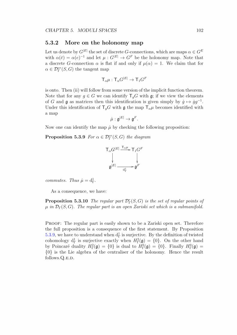
CHAPTER 5. MODULI SPACES 102
5.3.2 More on the holonomy map
Let us denote by G|E| the set of discrete G-connections, which are maps α ∈ GE
with α(e) = α(e)−1 and let µ : G|E| → GF be the holonomy map. Note thata discrete G-connection α is flat if and only if µ(α) = 1. We claim that forα ∈ DvrΓ (S,G) the tangent map
Tαµ : TαG|E| → T1G
F
is onto. Then (ii) will follow from some version of the implicit function theorem.Note that for any g ∈ G we can identify TgG with g; if we view the elementsof G and g as matrices then this identification is given simply by g 7→ gg−1.Under this identification of TgG with g the map Tαµ becomes identified witha map
µ : g|E| → gF .
Now one can identify the map µ by checking the following proposition:
Proposition 5.3.9 For α ∈ DvrΓ (S,G) the diagram
TαG|E|
Tαµ // T1GF
g|E|
d1Γ
// gF
,
commutes. Thus µ = d1Γ.
As a consequence, we have:
Proposition 5.3.10 The regular part DrΓ(S,G) is the set of regular points ofµ in DΓ(S,G). The regular part is an open Zariski set which is a submanifold.
Proof: The regular part is easily shown to be a Zariski open set. Thereforethe full proposition is a consequence of the first statement. By Proposition5.3.9, we have to understand when d1
Γ is surjective. By the definition of twistedcohomology d1
Γ is surjective exactly when H2Γ(g) = 0. On the other hand
by Poincare duality H2Γ(g) = 0 is dual to H0
Γ(g) = 0. Finally H0Γ(g) =
0 is the Lie algebra of the centraliser of the holonomy. Hence the resultfollows.Q.e.d.

CHAPTER 5. MODULI SPACES 103
Regular elements
We need a refinement of the discussion in the last paragraph for Γ = Γg. Wealso need some properties of centralisers of elements. Let us begin with somedefinitions.
Definition 5.3.11 [Singular and regular elements] Let G be an alge-braic group. We say an element g of G is singular if there exists a subgroupK such that dimZ(K) > 0 and such that g ∈ [K,K], and regular otherwise.
The reader is invited to check that for SU(2) the set of singular elementsis the centre. A real split element in SLn(R) is singular, if some product ofeigenvalues is equal to 1. We now prove
Proposition 5.3.12 Let µ be the map from G2g to G given by
(a1, b1, . . . , ag, bg) 7→i=g∏i=1
[ai, bi].
Then every regular element in G is a regular value of µ.
Proof: As a first computation, let ν be the map from Gk to G,
(c1, . . . , ck)→ c1 . . . ck.
Identifying TxG with g by the map u→ g−1.u, we obtain that Tν from gk tog is given by
(u1, . . . uk) 7→i=k∑i=1
(ad(ci+1 . . . ck)−1ui.
A similar computation for µ yields that
Tµ(u1, v1, . . . , ug, vg)
=
i=g∑i=1
ad(∏j>i
[ai, bi])−1
(ad(biaib−1i ).ui + ad(biai).vi − ad(biai).ui − ad(bi).vi)
=
i=g∑i=1
ad(∏j>i
[ai, bi])−1
(ad(biaib−1i )(1− ad(bi))ui + ad(bi)(ad(ai)− 1).vi)
=
i=g∑i=1
(ad(Ai)(1− ad(bi))ui + ad(Bi)(ad(ai)− 1).vi,

CHAPTER 5. MODULI SPACES 104
where
Ai = (∏j>i
[ai, bi])−1bi.ai.b
−1i , Bi = (
∏j>i
[ai, bi])−1bi.
Observe now that the image of the endomorphism of g given by u → (1 −ad(c))u is the orthogonal — with respect to the ad invariant metric – of thelie algebra of Z(c). It follows that the orthogonal of the image of Tµ is the Liealgebra of
H =
i=g⋂i=1
Z(AiaiA−1i )
i=g⋂i=1
Z(BibiB−1i ) = Z〈a1, b1, . . . , ag, bg〉.
It follows that (a1, b1, . . . , ag, bg) is a regular element for µ if and only if thecentraliser of the group generated by these elements is finite.
Therefore, denoting m = (a1, . . . , ag) and Λ(m) = 〈a1, . . . , ag〉, then m is asingular point for µ if dim(Z(Λ(m))) > 0. Observe moreover that µ(m) belongsto [Λ(m),Λ(m)]. By definition, µ(m) is a a singular point in G. Q.e.d.
5.3.3 The Zariski dense part is Zariski open and non-empty
It follows from Corollary 5.3.5 that DzdΓ (S,G) is Zariski open. We will nowprove that it is non-empty. We will give a complete proof only for G = SLn(R)
Lemma 5.3.13 Let G be a semi-simple algebraic group, then there exist twoelements in G that generates a Zariski dense group.
We will only prove this lemma for G = SLn(R) and admits the result forgeneral semi-simple groups. We say that a matrix a ∈ SLn(R) is R-split if it isdiagonalisable with distinct real eigenvalues.
Proof: Let a be any real split matrix. Suppose that, using the notation ofProposition 5.3.4, we have W ∈ Fixk(a). Then W is generated by eigenvectorsof a (for the adjoint action): more precisely, if ei is the basis of eigenvectorsof a in Rn, and ei the dual basis, then W is generated by elements of theform ej ⊗ ei. Thus by choosing the eigenvectors carefully it is possible to findanother split matrix b such that Fixk(a) ∩ Fixk(b) = ∅ for all 0 < k < dim g.Then the lemma follows from Proposition 5.3.4. Q.e.d.
Now we can prove

CHAPTER 5. MODULI SPACES 105
ab a
b
Figure 5.1: A flat discrete connection on a surface of genus 2
genus = 2
genus 2
Figure 5.2: Very regular connections for higher genus

CHAPTER 5. MODULI SPACES 106
Proposition 5.3.14 let G be an algebraic semi-simple group. Let S be asurface of genus greater than 1. Then DvrΓ (S,G) is non-empty.
Proof: Choose a and b as in Lemma 5.3.13. For a pair of pants surface(in other words a sphere with three holes) one can explicitly write down aflat discrete connection such that the image of the holonomy representationcontains a and b and is therefore Zariski-dense. For example one can takethe flat discrete connection depicted in Figure 5.1.Gluing two pairs of pantswith this discrete connection as in Figure 5.2 yields a discrete connection on asurface of genus 2, whose holonomy representation still contains a and b andthus is still very regular. If S is a surface of genus > 2 then we can decomposeit along a disc into a surface of genus g− 1 with one hole and a torus with onehole. Gluing connections as in Figure 5.2 we obtain a very regular connectionon S by induction on g. Q.e.d.
5.3.4 The action is proper
We prove the second part of Theorem 5.2.6
Proposition 5.3.15 The group GV acts freely and properly on DzdΓ (S,G).
The stabiliser of one element is identified with the centraliser of the holon-omy. Hence the action is free on DvrΓ (S,G) which contains DzdΓ (S,G). Themost difficult part is to verify that the G-action is proper. We cannot provethis in general here, so let us consider two special cases. The trivial case isthe case where G is compact. In this case, any action of G is proper andthere is nothing to show. In the non-compact case one needs again some moreresults on algebraic groups. An elementary proof with linear algebra methodsis possible if we make two simplifications. Firstly, let us assume Γ = Γg. Thenwe have
MvrΓg(S,G) = Homvr(π1(S), G)
and GV = G. Thus the properness of the GV -action is equivalent to thefollowing statement:
(∗) Let ρnn∈N ⊂ Homvr(Ag, G) be a convergent sequence. Then any se-quence gnn∈N ∈ G for which gnρng
−1n also converges, is bounded.
Let D ⊂ P(Cp))p/Sp be the set of p lines in Cp that forms a direct sum. Letus say two elements of D are transerse if no line in one element is containedin a proper subspace generated by lines of the other element.

CHAPTER 5. MODULI SPACES 107
Now let us prove the statement (∗) in the case of G = SLp(C). For this wecan as well assume that ρn → ρ0 and that gnn∈N ∈ G satisfies gnρng
−1n → ρ1.
We need two lemmas
Lemma 5.3.16 There exist a, b ∈ π1(S) such that ρ0(a), ρ0(b), ρ1(a), ρ1(b) areall C-split and the axis’ of ρ0(a) (respectively ρ1(a)) are transverse to the axis’of ρ0(b) (respectively ρ1(b)).
Proof: We distinguish two cases depending on whether ρ0 and ρ1 are conju-gate or not. In the former case it suffices to choose a and b in such a way thatρ0(a) and ρ0(b) are C-split with distinct axis. Now the set of C-split elementsof G is Zariski-open and non-empty and thus contains an element ρ0(a) fromthe Zariski-dense subset ρ0(Ag). Moreover, the set of C-split elements of Gwith axis’ transverse to a given element of D is still Zariski open and thisallows us to chose b. This settles the case where ρ0 and ρ1 are conjugate. Inthe other case it follows from Proposition 5.3.6 that (ρ0× ρ1)(π1(S)) is Zariskidense in G×G. Then the argument is reduced to the first case. Q.e.d.
Let us choose a and b as in the lemma. As ρn(a) → ρ0(a) and the setof C-split elements in G is open, we may assume that ρn(a) is C-split for alln ∈ N.
Let αn ∈ D denote the set of axis’ of ρn(a). Then αn → α0, where α0 is theset of axis’ of ρ0(a). Similarly, gnαn → α1, where α1 is the set of axis’ of ρ1(a).
We now remark that we have a locally bounded map W from D to SLp(C),so that for any β ∈ D, W (β)· β = α1: we choose a metric on Cp and for anyβ ∈ D, W (β) to send unit vectors in the lines of β to unit vectors in the linesof α1. It follows that we can write
gn = v−1n tnun,
where tn is diagonal with respect to a basis of eigenvectors of α1, un = W (αn),and vn = W (gnαn). Since W is a locally bounded map, we can reduce ourdiscussion to the case where gn are diagonal matrices with respect to a basisof eigenvectors of α1 = α0.
For that we need the following lemma:
Lemma 5.3.17 Let gnn∈N be an unbounded sequence of diagonal matricesin SLp(C). Let xnn∈N be a sequence of elements of P(Cp) which convergesto a line, which is not included in a coordinate hyperplane. Then gnxnn∈Nconverges (after taking subsequences) to a line contained in a coordinate hy-perplane.
CHAPTER 5. MODULI SPACES 108
Proof: Let first give the proof for p = 2. We then have gn = diag(λn, λ−1n )
and we may assume that λn → ∞. If xn = [an : bn] converges to [a : b] witha, b 6= 0. Then
gnxn = [λnan : λ−1n bn]→ [1 : 0].
For the general case, we may as well assume – after possibly permuting theaxis’ and choosing subsequences – that if gn = diag(λ1
n, . . . , λpn), then for some
q, with 1 < q ≤ p,
• λknn∈N is bounded for k ≥ q,
• λknn∈N tends to ∞ is bounded for k < q,
Then it follows that, after taking subsequences, the limit of gnxnn∈N lies inthe hyperplane on which the last coordinate vanishes. Q.e.d.
Now we can finish the proof: we now use our hypothesis on b. Let βn, β0 andβ1 denote the set of axis’ of ρn(b), ρ0(b) and ρ1(b) respectively. Then gnβn → β1
and βn → β0. Write all elements of G as matrices with respect to a basis ofeigenvectors of α1 = α0. Then the matrices gn ∈ SLp(C) are diagonal. Alsoas β0 is transverse to α0 = α1, each line in βn converges to an axis’, whichis not included in a coordinate hyperplane. Thus, by the lemma, if gn wereunbounded then gnβn would converge to an element in D not transverse toα1. But this contradicts the choice of a and b. Therefore gnn∈N must bebounded. This finishes our indication of the proof of (iii).
Hint of the proof in the general case. We just sketch here how the generalproof works. First we need the following fact about actions of algebraic groups:to show that an algebraic action of an algebraic group on an algebraic varietyis proper, it suffices to show that the orbits are closed. Indeed, by Rosen-licht theorem [Ros63] the action is stratified in the following sense: there is asequence of Zariski closed sets
Vn ⊂ Vn−1 ⊂ Vn−2 ⊂ . . . ⊂ V1 ⊂ V0 = V,
such that the action on Vi \ Vi+1 is proper.In our case, the fact that the orbit are closed follows from Corollary 5.3.7:
by this corollary, the G-orbit of a representation ρ, is
Vρ = ρ | ∀γ ∈ π1(S) Tr(ρ(γ)) = Tr(ρ(γ)).

CHAPTER 5. MODULI SPACES 109
5.3.5 The moduli space and its tangent space
We prove the third part of Theorem 5.2.6.
Proposition 5.3.18 The quotient
Mzd(S,G) := DvrΓ (S,G)/GV
is a manifold of dimension −χ(S) dimG whose tangent space at the class of arepresentation [ρ] is canonically identified with H1
ρ(g).
Proof: We have already proved that DvrΓ (S,G) is a submanifold on whichthe group GV acts freely and properly. Hence the quotient is a submanifoldand it remains to understand its tangent space.
Let us denote by G|E| the set of discrete G-connections, in other words mapsα ∈ GE with α(e) = α(e)−1 and let µ : G|E| → GF be the holonomy map.
Similarly, the action of G gives rise to an orbit map gV → TαG|E| and the
complexgV → TαG
|E| → Tµ(α)GF
can be identified using Proposition 5.3.9 with the complex
gVd0
Γ−→ gEd1
Γ−→ gF .
Thus the tangent space at [α] becomes identified with the quotient of ker d1Γ
by the image of d0Γ, which is precisely H1
α(g).It remains to compute the dimension of Mzd(S,G). We know that
dimMzd(S,G) = dimH1ρ(g).
On the other hand, by using Proposition 4.1.12,
dim(H0Γ(g))− dim(H2
Γ(g)) + dim(H2Γ(g)) = −χ(S) dim(g).
Since for elements in Dvr(S,G), the cohomology groups H0Γ(g) H2
Γ(g) vanish,the formula for the dimension of Mzd(S,G) follows. Q.e.d.
5.3.6 The complement of the Zariski dense part
We prove the final part of Theorem 5.2.6
Proposition 5.3.19 The complement of DzdΓ (S,G) in DzdΓ (S,G) is a finiteunion of GV -orbits union of algebraic manifolds of the form DΓ(S,H), whereH varies over the algebraic subgroups of G. It has Hausdorff dimension strictlyless than the dimension of DzdΓ (S,G).

CHAPTER 5. MODULI SPACES 110
Proof: We only sketch the proof here. By construction, for every homo-morphism ρ not in DzdΓ , there exists an algebraic group H which containsρ(Γ). Hence, the first part of the statement follows from the following fact:there exists finitely many conjugacy classes of maximal algebraic subgroup ofa semi-simple group. Q.e.d.
5.4 Connected components
5.4.1 Connected components I: the compact case
For general Lie groups G, the moduli space M(S,G) need not be connected.However, in some favourable cases this is indeed the case. For example onehas:
Theorem 5.4.1 If G is a compact, connected, simply-connected Lie groupwith finite centre, then M(S,G) is connected.
We will only proof the theorem when G = SU(2). The general case requiresa different proof from what we explain now:
To prove Theorem 5.4.1 we fix a genus g and consider once again the mapµ : G2g → G given by (ai, bi) 7→
∏[ai, bi]. Then M(S,G) = µ−1(1)/G and
thus M(S,G) will be connected if µ−1(1) is connected.Observe now that – in the case G = SU(2) – the set of singular elements is
the centre of G.It turns out that it is useful to study µ−1(g) for g 6= 1 first. Let T be the
maximal abelian subgroup of G – that is the group of diagonal matrices. LetC be the set of elements g such that dimZ(g) = dimT .
Lemma 5.4.2 The set C is dense, connected and is simply connected.
Proof: We can write
C = g ∈ G | i Tr(g) ∈]− 2, 2[.
Let ϕ : g → iTr(g). Note that ϕ is a fibration from C to its image and.Moreover the fibres of ϕ restricted to C are simply connected: they are home-omorphic to CP1. The lemma follows Q.e.d.
We also need the following lemma.
Lemma 5.4.3 The set µ−1(C) ⊂ G2g is connected.
CHAPTER 5. MODULI SPACES 111
Proof: Let us first consider the set R0 of elements which are critical pointsof µ. An element ρ is a critical point of µ, if its centraliser is not finite. Itfollows that R0 is included in the finite union of G-orbits of sets of the formH2g where H is a subgroup of G of positive codimension. It follows that R0
is included in a finite union of submanifolds of codimension greater than 2.Hence W = G2g \ R0 is open and connected. By definition µ restricted to Wis a submersion. Now µ−1(C) = W \ µ−1Id,−Id. Let
J = µ−1Id,−Id ∩W
has codimension equal to the dimension of SU(2) that is 3. It follows thatµ−1(C) is connected. Q.e.d.
For a regular element the connectedness of the fibre is easy to prove:
Lemma 5.4.4 If G = SU(2) and g ∈ C, then µ−1(g) is connected.
Proof: Let E := µ−1(G \ C). Then the restriction µ : E → G \ C is afibration. By Lemma 5.4.2 the base G \ C is simply connected and clearly Eis connected. Now the long exact homotopy sequence of µ ends with
. . .→ π1(G \ C)︸ ︷︷ ︸=0
→ π0(µ−1(g))→ π0(E)︸ ︷︷ ︸=0
→ π0(G \ C)→ 0.
Thus π0(µ−1(g)) = 0 as claimed. Q.e.d.
Of course 1 is a very singular element. However, using the fact that theregular elements are dense, we can deduce Theorem 5.4.1 from the followingapproximation result:
Lemma 5.4.5 Let K,P be topological spaces, K compact and let µ : K → Pbe a continuous map. Suppose that xnn∈N is a sequence in K such thatµ−1(xn) is connected for all n ∈ N. If xn → x0 then µ−1(x0) is also connected.
Exercise 5.4.6 Prove Lemma 5.4.5.
Now we may choose K := G2g, P = G, µ as before and xn a sequence ofregular elements converging to the identity in order to deduce Theorem 5.4.1.
CHAPTER 5. MODULI SPACES 112
5.4.2 Connected Components II : an invariant
Notice that the simple connectedness of G entered crucially in the proof (viathe long exact sequence of the fibration over the regular elements). Thus if wedrop this assumption then it is not surprising that Theorem 5.4.1 fails. Moreprecisely, let G be a connected semisimple compact Lie group, not necessarilysimply connected. Denote by π : G → G its universal covering. We mayidentify π1(G) with the fibre over 1. Then π1(G) becomes a normal discrete
subgroup of G with G/π1(G) = G and π gets identified with the canonicalquotient map.
Exercise 5.4.7 Show that a discrete normal subgroup Γ of a connected topo-logical group H is central and deduce that π1(G) ⊂ Z(G). (Hint: For γ ∈ Γconsider the conjugation map cγ : H → Γ given by h 7→ hγh−1.)
Construction of the invariant
We construct a mapχ :M(S,G)→ π1(G)
constant on connected components. The construction depends on some choicesand runs as follows.
1. We fix a filling ribbon graph Γ in S.
2. We choose a discrete flat connection on Γ, that is a collection ∇ =gee∈E so that g(e) = (g(e))−1, where E denotes the edges of Γ, repre-senting the element [∇] of M(S,G).
3. For every e ∈ E choose a lift ge ∈ G of ge in such a way that ge = ge−1.
Then ∇ = gee∈E defines a non-flat discrete G-connection on Γ.
4. For every face, we choose a vertex – called a base point – in the boundaryof the face, , so that we can define the holonomy of a face.
If F stands for the set of faces of Γ, we finally define
χ([∇]) :=∏f∈F
Hol∇(f).
One has to check that this is well-defined and independent of the choices made.We first prove
Proposition 5.4.8 For every face f , the holonomy Hol∇(f) takes value inπ1(G). Moreover

CHAPTER 5. MODULI SPACES 113
1. Hol∇(f) is independent of the choice of the base point of the face f ,
2.∏
f∈F Hol∇(f) is independent of the choice of the lift g,
3.∏
f∈F Hol∇(f) is invariant under gauge transformations.
Proof: First let us check that Hol∇(f) takes values in π1(G): As∇ is flat, theholonomy Hol∇(f) is trivial and thus π(Hol∇(f)) = 1. Now let us check thatHol∇(f) does not depend on the choice of lift: indeed, if we take another liftge′ with ge
′ = geγ for some γ ∈ π1(G), then we also have to take ge′ = γ−1ge
−1.But by Exercise 5.4.7 the group π1(G) is abelian and thus γ and γ−1 cancelin the product over all faces. (Recall that every edge is contained in preciselyone face.) Similarly, Hol∇(f) does not depend on the base point and is gauge-invariant. We leave this to the reader.Q.e.d.
One finally checks that∏
f∈F Hol∇(f) is invariant under subdivision andthus that it is independent of the choice of Γ. From this it follows that χ[∇]is well defined.
Now let us discuss the fibres of the map χ. If we construct χ using thestandard ribbon graph Γg, then it is easy to see that χ−1(α) is precisely thesubset of the representation variety of the fundamental group of the puncturedsurface π1(S \ ∗) with values in G given by the condition that the holonomy
around the puncture is given by α. Using the fact that G is simply-connected,a similar argument as in the proof of Theorem 5.4.1 will show that χ−1(α) isconnected for all α. This proves:
Theorem 5.4.9 If G is a connected semisimple compact Lie group, then theconnected components of M(S,G) are in one-to-one correspondence with theelements of π1(G).
Indeed, the correspondence is precisely given by the map χ above.
5.4.3 Connected components III: Milnor-Wood inequal-ity
For non-compact Lie groups the statement of Theorem 5.4.9 fails. This can al-ready be seen in the simplest example: G = SL2(R). Indeed, π1(PSL2(R)) ∼= Zis infinite, and thus Theorem 5.4.9 would predict an infinite number of con-nected components for M(S,G). However, this contradicts the fact that an

CHAPTER 5. MODULI SPACES 114
algebraic variety – such as Homzd(π1(S), G) – has only finitely many connectedcomponents. Therefore the problem to determine the number of connectedcomponents of M(S,G) cannot be solved by counting elements of the funda-mental group unless G is compact.
It also turns out that in some cases – and we shall only see the case G =PSL2(R) – the Euler class of the representation, which is a priori bounded bythe argument above, can be explicitly bounded.
Theorem 5.4.10 [Milnor-Wood inequality] Let G = PSL2(R). Thenfor any [∇] ∈M(S,G),
|χ([∇])| ≤ −χ(Sg) = 2g − 2.
The universal cover of PSL2(R)
We first observe that PSL2(R) admits a retraction by deformation on the sub-group of rotation SO(2,R), since PSL2(R)/SO(2,R) is the Poincare disk. Thus
π1(PSL2(R)) = π1(SO(2,R)) = Z.
Then, the universal cover of PSL2(R) can be constructed as follows. Observethat SL2(R) acts on the circle T1 through the identification with the projectiveline
T1 ∼ RP1 = (R2 \ 0)/R∗.Let now π : R → T1 be the universal covering of the circle given by t →
exp(2πit). Let G be the subgroup of diffeomorphisms ϕ of R lifting the actionof G = PSL2(R):
G := g ∈ Diff(R) | ∃h ∈ PSL2(R), π g = h π.By construction, we have a group homomorphism π∗ from G to G = PSL2(R)and we have.
Proposition 5.4.11 The group G is the universal cover of G = PSL2(R) andπ∗ is the covering map.
Proof: We observe that the preimage of SO(2,R) is the group of translations.It follows from this observation that G is connected and simply connected sinceit retracts on the group of translations. Q.e.d.
Proposition 5.4.12 Let G = PSL2(R). There exists a – non-continuous –
section σ : G → G of the universal covering of G such that for all x ∈ R andg ∈ G,
|σ(g).x− x| ≤ 1. (5.1)

CHAPTER 5. MODULI SPACES 115
Proof: Assume first that g has a a fixed point in x0. Let y0 a lift of x0.We choose σ(g) so that σ(g)(y0) = y0. Thus, since σ(g) is increasing, we haveσ(g)[y0, y0 + 1] = [y0, y0 + 1]. Thus, using the periodicity of σ(g), Inequality(5.1) holds.
Assume now that g has no fixed point. Let σ(g) be a lift of g, so that|σ(g)(0)| ≤ 1
2. Since x → |σ(g) − x| is continuous and never takes an integer
value – since g has no foxed points, it follows that Inequality (5.1) holds.Q.e.d.
Proposition 5.4.13 For every g and h in PSL2(R) and x ∈ R,
|[σ(g), σ(h)]x− x| ≤ 2. (5.2)
Proof: We first notice that since every element σ(g) is a continuous lift of adiffeomorphism, we have
|x− y| ≤ 1 =⇒ |σ(g)(x)− σ(g)(y)| ≤ 1. (5.3)
By Inequality (5.1)
|σ(h)(z)− z| ≤ 1. (5.4)
Thus using Inequality (5.3), with z = x and y = σ(h)(x), we have
|σ(g)(x)− σ(g)(σ(g)(x)| ≤ 1.
Finally taking y = σ(g)(x) in Inequality (5.4), we have
|σ(g)(x)− σ(h)(σ(g)(x)| ≤ 1.
Then,
|σ(g)σ(h)(x)− σ(h)σ(g)(x) ≤ |σ(h)σ(g)(x)− σ(g)(x)|+|σ(g)(x)− σ(h)(σ(g)(x)|
≤ 2.
The Proposition follows. Q.e.d.
A first inequality
In order to bound the number of connected components of the moduli spacewe consider, as in the compact case, the map χ : M(S,G) → π1(G) ∼= Z.Then we have:

CHAPTER 5. MODULI SPACES 116
Lemma 5.4.14 [Fake Milnor-Wood inequality]Let G = SL2(R). Then for any [∇] ∈M(S,G),
−2g ≤ χ([∇]) ≤ 2g.
Proof: We compute χ via the standard ribbon graph Γg. Suppose [∇] isrepresented by labellings a1, b1, . . . , ag, bg ∈ G at the 2g edges. Let σ be the
section of the universal covering G→ G constructed in Proposition 5.4.12 andput ai := σ(ai), bi := σ(bi). Then
|χ([∇])| =g∏i=1
|[ai, bi]|.
We obtain inductively,
|χ([∇])x− x| ≤ |[a1, b1][a2, b2] · · · [ag, bg]x− [a2, b2] · · · [ag, bg]x)|+ · · ·+ |[ag, bg].x− x|.
Now by Inequality (5.2), each of the g summands is bounded by 2 and thus
|χ([∇])x− x| ≤ 2g,
from which the lemma follows. Q.e.d.
Proof of the Milnor-Wood inequality
Actually, we can improve the bound on |χ([∇])| by “stabilising it” and get theMilnor-Wood inequality.
Proof: For any surface S we have |χ(∇)| ≤ χ(S) + 2. Consider now an n-sheeted covering Sn → S. View the elements ofM(S,G) as equivalence classesof representations. Any representation ρ : π1(S)→ G lifts to a representationρn : π1(Sn)→ G. Now χ([ρn]) = nχ([ρ]) since a preimage of a ribbon graph asn times as many faces as the original ribbon graph and χ(Sn) = nχ(S). Thus
|χ([ρ])| = 1
nχ([ρn]) ≤ 1
n(−χ(Sn) + 2) = −χ(S) +
2
n.
As n was arbitrary, the theorem follows. Q.e.d.

CHAPTER 5. MODULI SPACES 117
5.4.4 Connected components IV: Goldman’s work forPSL2(R)
For PSL2(R) the situation of connected components is pretty well understoodthanks to W. Goldman’s work. More precisely, the fact that the Milnor-Woodinequality is sharp follows from the following theorem of Goldman [Gol88]:
Theorem 5.4.15 [Goldman] Let G = PSL2(R). Then for all p with |p| ≤−χ(S) the fibre χ−1(p) is connected and non-empty. Thus M(S,G) has pre-cisely 4g − 3 connected components.
The maximal component χ−1(2g − 2) consists of discrete faithful represen-tations. It can be identified with Teichmuller space, the space of orientedhyperbolisations of the surface S. (A discrete faithful representation yields acovering action of π1(Sg) on the upper half plane PSL2(R)/PSO(2,R) and thusa hyperbolisation.) The minimal component χ−1(−2g + 2) corresponds to theTeichmuller space of S with opposite orientation. On these two components theaction of the mapping class group, that is the group of outer automorphismsModg := Out(π1(Sg)), is proper. On the other hand one has the followingconjecture of Goldman:
Conjecture 5.4.16 [Goldman] For every p 6∈ ±χ(Sg) the action of Modgon χ−1(p) is ergodic.
Thus there is a stark contrast between the spaces of maximal/minimal rep-resentations and the other components of the moduli space.
5.5 Comments, references and further read-
ings
Since we did not assume the students have any knowledge of algebraic groupsand algebraic actions, we only gave down-to-earth proofs for G = SL(n,R).The description of the character variety and its smooth points can be found infull generality in Rapinschuk–Benyash-Krivets–Chernousov, [RBKC96], Lubotzky-Magid [LM85] and incidentally in Goldman [Gol88, Gol84] and Bismut–Labou-rie [BL99]. The singularities are discussed in Goldman–Millson [? ].
The fact that the character variety is connected for simply connected com-pact or complex reductive groups is proved in Jun Li [Li93], it uses the iden-tification of the character variety with stable holomorphic bundles due toNarasimhan–Seshadri (for the unitary case) [NS65] extended to the generalcase by Ramanathan [Ram75]. The proof given in these notes for SU(2) is

CHAPTER 5. MODULI SPACES 118
also in [Gol88], but cannot be extended straightforwardly to all compact sim-ply connected Lie groups. It would be nice nevertheless to have a proof inthis spirit of the connectedness of M(S,G) in this spirit when G is simplyconnected.
The remark that only finitely may values of characteristic classes can beobtained for flat G-bundles on a given manifold is attributed independently toMilnor and Lusztig. Milnor-Wood inequality is proved by Milnor for PSL2(R)and Wood for circle bundles in [Woo71, Mil58]. Turaev [Tur84] extended thisinequality for symplectic groups, and later Burger–Iozzi–Wienhard [BIW03]and Bradlow–Garcıa-Prada–Gothen extended it to all isometry groups of her-mitian symmetric spaces [BGPG06].-
The classification by Goldman of connected components for G = PSL2(R) isin [Gol88]. Goldman’s ergodicity conjecture about non-maximal componentsfor non-G = PSL2(R) is the pendant of his ergodicity theorem for G = SU(2)[Gol97].
The first examples of connected components with the same characteristicclasses are due to Goldman in [Gol88] for lifts of representations in SL(2,R),interesting examples are also due to Hitchin for PSLn(R), for n ≥ 3, [Hit92].One of the most interesting case is the character variety for G = Sp(4,R)whose connected components have been counted by Garcıa-Prada–Mundet iRiera [GPiR04] and described topologically by Guichard–Wienhard [GW10].Concerning connected components let us remark that it follows from Goldman–Millson Rigidity Theorem [GM87] that a connected component may containno Zariski dense representation and have a smaller dimension than expected,thus Zariski dense representations are not always dense.
Atiyah–Bott’s [AB83] foundational paper – completed by Daskalopoulos in[Das92] – gives further topological information using a Morse theoretic ap-proach, and this approach has led to many interesting further developments.

Chapter 6
Symplectic structure of themoduli spaces
In this chapter, we concentrate on the symplectic nature of the representationvariety M(S,G). After constructing the symplectic structure, we describeseveral related Poisson algebras of observables: the Goldman algebra of Wilsonloops and spin networks observables.
Finally, following Witten, we compute the volume of M(S,G) when G is acompact Lie group.
6.1 Universal connections and smooth struc-
tures
In this preliminary section, we relate the smooth part of the moduli space withsmooth family of connections.
6.1.1 Lifting Lemmas
Lifting small neighbourhoods
For a bundle E over S denote by AE the affine space of connections and byAE := Ω1(S,End(E)) the underlying vector space.
Lemma 6.1.1 [Lifting Lemma] Let [ρ0] be an element ofMzd(S,G). Thenthere exist a neighbourhood U of [ρ0] in Mzd(S,G), a bundle E over S and asmooth map f : U → AE whose image consists of flat connections so that theholonomy representation of f([ρ]) is given by [ρ].
119
CHAPTER 6. SYMPLECTIC STRUCTURE 120
Proof: Fix a good covering of S. If X zd denotes the space of G-local systemswith respect to this covering, which represent Zariski dense representations,then the projection X zd →Mzd(S,G) is a locally trivial principal bundle. Inparticular, it admits local sections. Thus we find a neighbourhood U of [ρ0]and a section σ : U → X zd.
We furthermore assume that U is diffeomorphic to a ball.For every point in U we have a locally constant G-valued cocycle on S with
respect to our chosen covering. In other words, we have a G-valued cocycle onS×U , which is locally constant along S. Observe that a a cocycle give rises toa concrete bundle E on S×U together with a flat G-connection along S. (Notethat a local system really gives rise to a concrete bundle with connection, notjust an equivalence class, and that it does so in a smooth way).
Now, it suffices to show that this bundle is “constant” along U , or more pre-cisely that it is equivalent to the pullback of a bundle over S via the projectionπ : S × U → S. This follows from the contractibility of U .
Let us explain this fact in some more details: Let E0 := E|S×[ρ0], which is
a bundle over S×[ρ0] ∼= S. Let E := π∗0E0, where π0 : S×U → S×[ρ0] is
the canonical projection. Our goal is to construct a isomorphism F : E → Ewhich induces the identity on the base space S × U . For this, we take anyconnection on E - without any relation whatsoever to any of the connectionsoccurring before.
As U is a ball with centre [ρ0], we can join every point u ∈ U to [ρ0] by apath cu : [0, 1]→ U so that the map U × [0, 1]→ U given by (u, t) 7→ cu(t) issmooth. The bundle isomorphism F is defined by assigning to v ∈ E(s,u) itsimage by the holonomy along cu:
F (v) := Hols×cu(v).
Q.e.d.
As a byproduct we obtain the following result:
Corollary 6.1.2 If [∇0], [∇1] are in the same connected component of themoduli space Mzd(S,G), then they can be represented by connections on thesame bundle E.
6.1.2 Universal connections
We now elaborate on the Lifting Lemma and introduce the following device.
Definition 6.1.3 A universal connection is a connection ∇ on a bundle E overS ×Mzd(S,G) such that for every representation ρ belonging to Mzd(S,G),∇|[ρ]×S is a flat connection with holonomy conjugate to ρ.

CHAPTER 6. SYMPLECTIC STRUCTURE 121
The following result is a generalisation of the Lifting Lemma.
Theorem 6.1.4 [Universal connection] For every surface S and groupG there exists a universal connection ∇] over a bundle over S ×Mzd(S,G).
Proof: we use the notation and ideas of the proof of the Lifting Lemma.The initial remark of this proof is that a smooth map from an open set U to
AE is the same object as a smooth connection on E → S × U which is trivialalong s × U .
Therefore, assume that we have two open sets U and V in Mzd(S,G). Letf and g be two lifts from respectively U and V to AE. Let ∇U and ∇V
be the associated connections on S × U and S × V respectively. Then byhypothesis, for any m in U ∩ V , the connections ∇U |m×S and ∇U |m×S aregauge equivalent. Since the holonomies have Zariski dense image, the gaugeequivalence is unique. In other words, there exists a unique σm = σU,Vm in thegauge group of E → S so that
∇U |m×S = σ∗m∇V |m×S. (6.1)
From the uniqueness it follows that m → σm is continuous. Moreover, theconstruction given in the proof of the lifting Lemma yields that m → σ issmooth.
Let now Uii∈I be a covering of Mzd(S,G) by open sets such as in theLifting Lemma. From the uniqueness again, the collection of maps σU,Vm
defines a G-valued cocycle on E and a vector bundle E over S ×Mzd(S,G).Moreover each connection ∇i := ∇Ui gives rise to a connection on E|Ui and
by construction on Ui ∩ Uj we have by Equation 6.1
∇i|m×S = ∇j|m×S. (6.2)
We now produce a universal connection by setting
∇ =∑i
ϕi∇i,
where ϕi is a partition of unity subordinated to the covering.Q.e.d.
The final statement of this section is an elaboration on these ideas andfollows from the proof.

CHAPTER 6. SYMPLECTIC STRUCTURE 122
Proposition 6.1.5 Let ∇] be a universal connection. Let M be a manifold,E be a vector bundle over M over M × S, ∇ be a connection on E suchthat for any point m in M , ∇|m×S is a flat connection whose holonomyrepresentation [ρ]m has almost Zariski dense image. Let Φ be the map fromM × S to Mzd(S,G)× S given by (m, s)→ ([ρ]m, s). Then
1. The map Φ is smooth.
2. There exist an element σ of the gauge group of E, so that for any m inM ,
Φ∗∇]|m×S = σ∗∇|m×S.
6.2 The symplectic form
The aim of this subsection is to equip the Zariski dense part Mzd(S,G) ofthe moduli space with a symplectic structure in the sense of the followingdefinition:
Definition 6.2.1 A symplectic structure on a manifold M of dimension 2nis a 2-form ω ∈ Ω2(M) which satisfies
(i) dω = 0, in other words ω is closed;
(ii) ω is fibrewise non-degenerate, in other words ω∧n is nowhere vanishing.
The pair (M,ω) is then called a symplectic manifold.
Recall from Theorem 5.2.6 that the tangent space T[ρ]Mzd(S,G) can beidentified with the twisted cohomology group H1
ρ(g). On H1ρ(g) the intersection
form iρ defines a non-degenerate alternating bilinear form. These forms fittogether nicely:
Theorem 6.2.2 Let S be a surface of genus g ≥ 2. Then the intersectionforms iρ on T[ρ]Mzd(S,G) ∼= H1
ρ(g) fit together to a symplectic form ω onMzd(S,G).
Definition 6.2.3 The above symplectic form is called the Atiyah-Bott-Gold-man symplectic form on the representation variety.
Now we prove our theorem:
Proof: [of Theorem 6.2.2] As we have already seen in Theorem 4.1.8 that theintersection forms are non-degenerate, we have only to show that ω is closedand smooth.

CHAPTER 6. SYMPLECTIC STRUCTURE 123
It suffices to show that for any [ρ0] ∈ Mzd(S,G) there exists a neighbour-hood U of [ρ0] such that ω|U is the pull-back of a smooth exact form. ByLemma 6.1.1 we may assume that there exists a bundle E and a smooth mapf : U → AE such that the holonomy representation of f([ρ]) is given by [ρ].On the underlying vector space AE we have a pairing Ω given by
Ω(α, β) :=
∫S
Tr(α ∧ β),
whereTr(α ∧ β)(x, y) = TrEnd(E)(α(x)β(y)− β(y)α(x)).
As the tangent space of AE at any point is identified with AE, Ω induces asmooth 2-form on AE. If ∇0 is any fixed connection on E and ξ is the one-formon AE given by
ξ∇(α) =
∫S
Tr((∇−∇0) ∧ α),
then Ω = dξ. Thus Ω is a smooth exact 2-form on AE. From the definition ofthe intersection form we see that ω|U = f ∗Ω and the theorem follows. Q.e.d.
6.3 Classical mechanics and observables
In classical mechanics symplectic manifolds (M,ω) model phase spaces. In thiscontext, elements of C∞(M) are regarded as observables. The dynamics of theobservables can be expressed in term of the Poisson bracket, which is definedas follows: using the symplectic form we can associate to every observable f avector field Hf called the Hamiltonian vector field of f and given by
df(u) = ω(u,Hf ).
Then the Poisson bracket ·, · : C∞(M)× C∞(M)→ C∞(M) is defined by
f, g := ω(Hf , Hg) = dg(Hf ).
The set of observables has the following algebraic structure:
Proposition 6.3.1 If (M,ω) is a symplectic manifold the (C∞(M), ·, ·, ·)is a Poisson algebra, in other words enjoys the following properties
• (C∞(M), ·, ·) is a Lie algebra ,
• (C∞(M), ·) is a commutative associative algebra,

CHAPTER 6. SYMPLECTIC STRUCTURE 124
• the two structures are compatible in the sense that Leibniz identity holds
f, gh = hf, g+ gf, h.
Of course, it is rather naive to call any arbitrary function onM an observable- at least from a physical point of view. Namely, one is usually only interestedin observing some special quantities like energy, momentum etc. and not justarbitrary functions. Thus there should be a subset of C∞(M) consisting ofinteresting observables. As the dynamics of the observable is governed by thePoisson algebra structure, a collection of interesting observables of M shouldbe a Poisson subalgebra of C∞(M). In the case of the representation variety,there are various such subalgebras of geometric interest. In this subsection andthe next we discuss two such subalgebras, which are related to the topology ofthe surface S and feature prominently in topological quantum field theory.
6.4 Special observables I: Wilson loops and
the Goldman algebra
We first recall some elementary facts about loops and conjugacy classes in thefundamental group. The free homotopy class of a loop is the homotopy classof the loop as a map from the circle to the surface S.
Choosing a base point x in S and path α from x to a point in the loop γ, weobtain a loop η = α.γα−1 based at x and thus an element in π1(S, x). Differentchoices of the connecting path lead to conjugate elements in π1(S, x). Moregenerally, a free homotopy class of loop defines a conjugacy class in π1(S, s).Conversely every conjugacy class in π1(S, x) defines a free homotopy class ofloop. We denote by [γ] the conjugacy class of γ in π1(S, x), or equivalently thefree homotopy class of the loop γ.
Note finally that if ρ is a representation of π1(S, s) in G, the conjugacyclass [ρ(γ)] of ρ(γ) in G only depends on the conjugacy classes of γ and ρ.This remark allows us the following definition since traces only depends onconjugacy classes.
Definition 6.4.1 [Wilson loops] Let [γ] be a conjugacy class in π1(S). Letλ be a linear representation of G. The following function
w[γ] :Mzd(S,G)→ R, [ρ] 7→ Tr(λ[ρ]([γ])),
is called, following physics literature, the Wilson loop associated to γ and λ.

CHAPTER 6. SYMPLECTIC STRUCTURE 125
Exercise 6.4.2 Let ∇ be the flat connection associated to λ and ρ. Let [γ]be a homotopy class of loop. Check that
w[γ]([∇]) = Tr(Hol∇(γ)).
In order to understand the dynamics of the Wilson loops it is importantto understand the structure of the Poisson algebra that they generate inC∞(Mzd(S,G)). For this it is enough to understand the Poisson bracket of twoWilson loops, as the general case can be reduced to this using the axioms of aPoisson algebra. In order to carry out this computation, we introduce anotherclosely related algebra, which can be defined in purely geometric terms.
Let GS be the real vector space spanned by the free homotopy classes ofloops, where the trivial loop is identified with zero.
We begin with a proposition. First we recall that if two oriented curves c1
and c2 in S meet transversely at a point x, we define εx(γ1, γ2) to be 1 if (c1, c2)is oriented and −1 otherwise. Then
Proposition 6.4.3 Let γ1, γ2 be two loops in S with transversal intersections.Then, the following element of GS
γ1, γ2 :=∑
x∈γ1∩γ2
εx(γ1, γ2)[γ1]xγ2].
only depends on the classes [γ1], [γ2]. Moreover, if we define [γ1], [γ2] :=γ1, γ2, then (GS, , ) is a Lie algebra.
This yields the following definition.
Definition 6.4.4 The Lie algebra (GS, ·, ·) is called the Goldman algebra.
The precise relation between the Goldman algebra and the Poisson algebragenerated by the Wilson loops depends on the target group G. For exampleone has:
Theorem 6.4.5 [Goldman] Let S be a surface, G a linear Lie group andlet [γ1], [γ2] be two free homotopy classes of loops in S with associated Wilsonloops w[γ1],w[γ2] ∈ C∞(Mzd(S,G)).
(i) If G = GL(n,R) then
w[γ1],w[γ2] = w[γ1],[γ2]
(ii) If G = SLn(R) then
w[γ1],w[γ2] = w[γ1],[γ2] −1
ni([γ1], [γ2])w[γ1]w[γ2],
where i([γ1], [γ2]) =∑
x∈γ1,γ2εx(γ1, γ2) denotes the algebraic intersection
number of γ1 and γ2 which only depends on the homotopy classes of [γ1]and [γ2].

CHAPTER 6. SYMPLECTIC STRUCTURE 126
Hamiltonian vector field of Wilson loops
Our first step in the proof Theorem 6.4.5 is to compute the Hamiltonian vectorfield of a Wilson loop. Thus let us fix a loop γ and denote by H := Hw[γ]
theHamiltonian vector field associated to the corresponding Wilson loop w[γ].
We identify T[ρ]Mzd(S,G) for [ρ] in Mzd(S,G) with H1ρ(g). Recall from
Definition 4.1.11 that this H1ρ(g) is the twisted cohomology of a certain bundle
with connection (Lg,∇g) whose typical fibre is the Lie algebra g of G.Thus H is represented by a class of closed 1-forms H∇ on S with values in
the bundle Lg. We are going to construct such a 1-form explicitly.We assume that G ⊂ GL(n,R) is reductive – as are our classical examples
SU(n), SLn(R). On Mn(R) we have a non-degenerate inner product given by(A,B) 7→ Tr(A,B). The reductivity assumption translates in the fact thatMn(R) splits as
Mn(R) = g⊕ g⊥.
From the point of view of bundle, we consider an associated G-bundle Eof rank n equipped with a flat connection, so that (Lg,∇g) is a subbundle ofthe bundle End(E). The above splitting translates in a parallel orthogonalsplitting
End(E) = Lg ⊕ L⊥g .Denote by X 7→ X the projection onto the first summand.
In order to simplify things, let us assume that γ is does not have any self-intersection.
We describe the step of the construction and first make the following choices.Let U be a tubular neighbourhood of γ and βγ a closed 1-form for with supportin U so that for any closed 1-form α defined on U and for any transverse curvec to γ ∫
U
α ∧ βγ =
∫γ
α, (6.3)∫c
βγ = i(c, x). (6.4)
Such a form βγ is easily constructed out of the derivative of a bump function.For any point x ∈ U , the holonomy Holγ(x) of a loop based at x and
freely homotopic to γ in U with respect to the connection ∇ = ∇g is anautomorphism of the fibre Ex. Observe that Holγ : U → End(E) is a welldefined section which is furthermore parallel (cf Exercise 3.3.11).
By a slight abuse of language we denote by Holγ ·βγ the 1-form with values
in Lg which vanishes outside U and is equal to Holγ · βγ, on U . One easilychecks that this form is closed.

CHAPTER 6. SYMPLECTIC STRUCTURE 127
We claim that the cohomology class of this form is the symplectic gradientof the Wilson loop.
Proposition 6.4.6 Let notation be as above. Then the class of Holγ · βγ inH1ρ(g) represents H∇.
Proof: We choose a family of ∇t a family of flat connections deforming∇ = ∇0. We denote by [∇] the tangent vector t = 0 to the curve inMzd(S,G)given by t→ [∇t]. We have a representative of [∇] given by
∇ =d
dt
∣∣∣∣t=0
(∇t −∇0) ∈ Ω1(S,Lg).
We want to computed
dt
∣∣∣∣t=0
tr(Hol∇t(γ)).
We consider γ as a Z periodic map from R to S. We choose a trivialisation ofγ∗E so that γ∗∇0 is the trivial connection D and write γ∗∇t = D +At. Let ∂
∂s
be the canonical vector field on R and
Bt(s) := At
(∂
∂s
).
Then by Proposition 3.3.12 the holonomy of ∇t is obtained by solving thefollowing linear ordinary differential equation
(∗) dX
ds= BtX.
More precisely, recall that the resolvent u, s→ tRsu of this equation is by defi-
nition such that X(s) := tRsuX(u) is the solution of (∗) with initial condition
X(u) at time u. Then,Hol∇t(γ) = tR1
0.
The method of the variation of constants yields
d
dt
∣∣∣∣t=0
Tr(Hol∇t(γ)) =d
dt
∣∣∣∣t=0
Tr(tR10) =
∫ 1
0
Tr(tR1+ss B(s)) ds,
where
B =d
dt
∣∣∣∣t=0
Bt(s) = ∇(∂f
∂s
).

CHAPTER 6. SYMPLECTIC STRUCTURE 128
We now interpret the right-hand side term and rewrite this integral as∫ 1
0
Tr(0R1+ss B(s)) ds =
∫ 1
0
Tr
(Hol∇0(γ)γ(s))∇
(∂γ
∂s
))ds (6.5)
=
∫γ
Tr(
Holγ ·∇)
(6.6)
=
∫γ
Tr(
Holγ · ∇)
(6.7)
In the last equality, we have used that Tr(au) = Tr(au) if u belongs to g. Letα be the 1-form defined on U by
α = Tr(Holγ · ∇).
Note that α is closed. It follows by Equation (6.3), that∫U
α ∧ βγ =
∫γ
α
Therefore combining the previous equations, we obtain that
d
dt
∣∣∣∣t=0
Tr(Hol∇t(γ) =
∫γ
α
=
∫U
α ∧ βγ
=
∫U
Tr(
Holγ∇)∧ βγ
= −∫S
Tr(
Holγ · βγ ∧ ∇).
Using the symplectic form ω on Mzd(S,G) we finally obtain
dwγ(ρ) = −∫S
Tr(Holγ · βγ ∧ ∇) = −ω(Holγ · βγ, ∇).
Thus by definitionH∇0 = [Holγ · βγ].
Q.e.d.
Exercise 6.4.7 Deduce Theorem 6.4.5 from Proposition 6.4.6.

CHAPTER 6. SYMPLECTIC STRUCTURE 129
6.5 Special observables II: Spin networks
A larger class of observables onMzd(S,G) which includes Wilson loops 6.4.1 asa special case can be constructed using embeddings of so-called spin networks.The starting definition is the following:
Definition 6.5.1 [Spin networks] A spin network S for G consists of thefollowing data
• an oriented graph Γ = ΓS = (V,E) called the underlying graph of S.
• for every e ∈ E, a vector space Ie = ISe and a representation λe = λSe :G→ Aut(Ie).
• for any v ∈ V , a linear map
iv = iSv ∈ Hom
⊗e∈E | e+=v
Ie,⊗
e∈E | e−=v
Ie
,
which intertwines the G-actions in the sense that for any g ∈ G,
iv
⊗e∈E | e+=v
λe(g)
=
⊗e∈E | e−=v
λe(g)
iv.We observe that the group GE naturally acts on the space of spin networks
with a common underlying graph. Namely, for every edge e we conjugate therepresentation by g(e), and for every vertex we perform the coherent trans-formation on the intertwiner. This action is called the gauge action on spinnetworks.
Definition 6.5.2 [Embedding of a spin network] Let S be a surfaceequipped with a bundle L. An embedding of the spin network S into S is bydefinition:
• an embedding of ΓS into S,
• for every vertex v in the underlying graph, an identification of LΨ(v) witha fixed vector space L.
We say two embeddings of two spin networks are equivalent under the gaugeaction are isotopic embeddings of spin networks if the corresponding embeddingof the underlying graph are isotopic. For instance, fixing the embedding of thegraph, and changing the identification of the fibres at images of vertices withL, yield isotopic embedding of spin network. An isotopy class is called anembedded spin network.

CHAPTER 6. SYMPLECTIC STRUCTURE 130
6.5.1 An observable on the space of all flat connections
Now, we shall define a function on the space of flat connections on L associatedto every embedding of a spin network in S.
Let S be a spin network and let Ψ : S → S be an embedding into somesurface S. Let∇ be a flat connection on some bundle L with fibre L. Using theidentification of LΨ(v) with L, for every edge e, holonomy H(e) := Hol∇(Ψ(e))becomes an element of G. Thus λe(H(e)) ∈ End(Ie). We now define
ΛΨ(∇) :=⊗e∈E
λe(H(e)) ∈ Aut
(⊗e∈E
Ie
).
On the other hand
IΨ :=⊗
v∈V iSv ∈ ⊗
v∈V
(Hom
(⊗e∈E | e+=v Ie,
⊗e∈E | e−=v Ie
))= Hom
(⊗v∈V
⊗e∈E | e+=v Ie,
⊗v∈V
⊗e∈E | e−=v Ie
)= End
(⊗e∈E Ie
)Then we can multiply
ΛΨ(∇) · IΨ ∈ End
(⊗e∈E
Ie
),
Thus we define an observable on the space of all flat connections by
fΨ : ∇ 7→ Tr(ΛΨ(∇) · IΨ).
Definition 6.5.3 [Spin network observable] The function fΨ describedabove is called the spin network observable to associated to Ψ.
Remark:
1. Observe that this construction extends the notion of a Wilson loop asa loop is nothing but an embedding of the trivial spin network whoseunderlying graph has one vertex and one edge and whose only intertwineriv is the identity.

CHAPTER 6. SYMPLECTIC STRUCTURE 131
An observable on Mzd(S,G)
The following proposition says that the spin network is a well defined observ-able on M
Proposition 6.5.4 [Invariance of the spin network] The value of fΨ
at ∇ is invariant under gauge action on ∇, and isotopies of the embedding ofthe spin network. Hence, it yields a function fΨ on Mzd(S,G)
Definition 6.5.5 [Spin network observable (bis)] By a new abuse oflanguage, we call again the corresponding function a spin network observable.
6.5.2 Poisson bracket of spin network observables
We define the space S of spin networks on S as the R-module generated bythe equivalence classes of spin networks - actually it should be a quotient ofthat space .... By the above definition, the map Ψ 7→ fψ extend to a linearmap
ev : S→ C∞(Mzd(S,G)).
We will now define a Lie bracket on S which generalises the Poisson bracketon the Goldman algebra. For this let S1, S2 be two spin networks and let
Ψ1 : S1 → S
Ψ2 : S2 → S.
be two embeddings. Assume that the images of the underlying oriented graphsΓ1,Γ2 intersect transversely. As in the case of the Goldman algebra we shalldefine for each intersection point x ∈ Γ1 ∩ Γ2 a sign εx and new spin networkS1]xS2 defined below as well as an embedding Ψx of this spin network. Wefinally define
[Ψ1,Ψ2] :=∑
x∈Γ1∩Γ2
εx ·Ψx.
Let us make this definition precise.
• The definition of εx is as in the case of the Goldman algebra: εx is 1 ifthe orientations of Γ1 and Γ2 are such that Γ2 crosses Γ1 at x from rightto left and −1 otherwise.
• The underlying graph of (S1]xS2,Ψx) does not depend on x and is justa transverse superposition of the underlying graphs of S1 and S2: its
CHAPTER 6. SYMPLECTIC STRUCTURE 132
vertices are the union of the vertices of Γ1 and Γ2 and all intersectionpoints of Γ1 and Γ2, its edges are connected components of
S1 ∪S2 \ (S1 ∩S2) ,
and the embedding is the one given by Ψ1 and Ψ2.
• Any edge is a subedge of an edge of either Γ1 or Γ2 and it is labelled bythe corresponding G-module.
• The vertices of Γ1 and Γ2 are labelled by the same intertwiners as before.
• Finally, suppose y is an intersection point of an edge e1 of Γ1 with an edgee2 of Γ2. Let (I1, λ1), (I2, λ2) be the corresponding G-modules. Then wehave to define an intertwiner iy : I1⊗I2 → I2⊗I1. Such intertwiners canbe constructed using the Lie algebra representations Dλj : g→ End(Ij),j = 1, 2: Assume that there exists a non-degenerate invariant bilinearform 〈·, ·〉 on g. For a simple Lie algebra we can take the Killing form,but such a form may also exist for non-simple Lie algebras, for examplegl(n,R). Let e1, . . . , ek be a basis of g which is orthonormal with respectto 〈·, ·〉. Then one checks that the Casimir intertwiner
4 :=k∑i=1
Dλ1(ei)⊗Dλ2(ei) ∈ End(I1 ⊗ I2)
is independent of the choice of orthonormal basis and intertwines thetensor product action of G on I1 ⊗ I2 with itself. Thus we define
iy :=
4, if y = xId, if y 6= x
This finishes the construction of (S1]xS2,Ψx). As in the case of Wilson loopsthe Poisson bracket of spin network observables is closely related to the Liebracket of embedded spin networks. In the case of GL(n,R) one has:
Theorem 6.5.6 Let G = GL(n,R) and let Ψ1,Ψ2 be embedded spin net-works in a surface S. Then the associated spin network observables fΨ1 , fΨ2 ∈C∞(Mzd(S,G)) satisfy
fΨ1 , fΨ2 = f[Ψ1,Ψ2].
We leave this theorem as a stimulating exercise for the reader. In particularone gets
Corollary 6.5.7 The associative algebra generated by ev(S) is a Poisson sub-algebra.

CHAPTER 6. SYMPLECTIC STRUCTURE 133
6.6 Volumes of moduli spaces
In this section, we compute the symplectic volume of the moduli space whenG is compact. This proof due to Witten [Wit91] will make use of the mainresult of our chapter on torsion which identifies the torsion and the symplecticvolume on cohomology groups.
6.6.1 Witten’s formula
Recall that the very regular part carries a symplectic form.
Theorem 6.6.1 [Witten’s formula] Let S be a surface of genus g and letG be a simply-connected simple compact Lie group with finite centre Z(G).Then the volume of the moduli space M(S,G) with respect to the symplecticform is given by
vol(M(S,G)) = |Z(G)|∑λ∈G
(vol(G)
dimVλ
)2g−2
,
where the volume of G is computed with respect to the Killing form, G is thethe set of finite dimensional representations λ of G and Vλ is the vector spaceassociated to λ.
Remarks:
1. [on normalisation] Given a symplectic manifold (M,ω) of dimension2d, the associated volume form is the Liouville volume 1
d!ωd.
2. In this theorem, everything – the symplectic form and the volume ofthe group – is computed with respect to the Killing form k. We couldhave chosen another normalisation. Let just see what happens when wechoose instead of k, the metric αk. Then
volα(G) = αdimG
2 vol(G),
andvolα(M(S,G)) = α(g−1) dimGvol(M(S,G)).
Hence the formula is homogeneous.
For reason that are going to be clearer in the next section, it is also quitenatural to choose 1
4π2k as in Witten’s’ original paper. This normalisation
CHAPTER 6. SYMPLECTIC STRUCTURE 134
is motivated by the fact that 14π2ω is integral (as we shall see below) and
is used by Witten. Therefore the original Witten formula reads as
vol∗(Mzd(S,G)) =
(1
2π
)−χ(S) dimG∑λ∈G
|Z(G)| · (vol(G))2g−2
(dimVλ)2g−2,
which differs from our formula precisely by the factor ( 12π
)−χ(S) dimG.
3. For G = SU(2), we have G ∼= N and dimVn = n. Moreover, Z(SU(2)) =
±1. The volume of G with respect to the Killing form is 252π2. Thus
we obtain
vol(S,M(SU(2))) = 2(2(5g−5)π4g−4)∞∑n=1
n−(2g−2).
We rather choose the metric 14π2k. Hence,
vol 14π2
(M(S,G)) = 2(2(5g−5)π4g−4)
26g−6π6g−6
∞∑n=1
n−(2g−2) =ζ(2g − 2)
2g−2π2g−2
where ζ(z) denotes the Riemann zeta function. In particular, the volumewith respect to this normalisation is rational.
The proof goes in two steps. The first step is to identify this measure witha measure obtained by disintegration in Proposition 6.6.3. The second step isto compute by induction in Proposition 6.6.6 the volume with respect to thismeasure.
6.6.2 Volume and the disintegrated measure
We first recall the definition of a disintegrated measure. In a presence of a mapbetween two measured spaces, there is a general way to construct a family ofmeasures on the fibres.
Proposition 6.6.2 Let (X, νX) and (Y, νY ) be finite measure spaces and letf : X → Y be a measurable map, such that f∗νX is absolutely continuous withrespect to νY , then there exists a unique measurable family of measures νyy∈Y ,where νy is a measure on f−1(y), such that for all measurable g : X → R theidentity ∫
X
g(x)dνX(x) =
∫Y
(∫f−1(y)
g(x)dνy(x)
)dνY (y).
holds.
CHAPTER 6. SYMPLECTIC STRUCTURE 135
The family νyy∈Y is said to be obtained by disintegration of (X, νX) and(Y, νY ) with respect to f .
In the next proof we will not use the full force of this result and just proveand use it in a geometric differential context.
We now interpret the symplectic volume using a disintegrated measure Letµ : G2g → G be the map given by
µ(a1, b1, . . . , ag, bg) =
i=g∏i=1
[ai, bi].
We equip G with the Killing form.
Theorem 6.6.3 Let ν be the disintegrated measure on µ−1. Then∫µ−1(Id)
ν =vol(G)
|Z(G)|
∫M(S,G)
ωn
n!,
where n = 12
dim(M(S,G)) and ω is the symplectic form on M(S,G).
Preliminaries
We first need to understand in a geometric differential way disintegration ofmeasures. This is the purpose of the next lemma.
Lemma 6.6.4 We use the same notation as in Proposition 6.6.2. When Xand Y are smooth, f is a submersion, and νX and νY come from volume formsΩX and ΩY , the measure νy also comes from a volume form Ωy. This familyof measures satisfy
ΩX = Ωy ⊗ ΩY ,
where we use the identification
det(TxX) = det(kerTxf)⊗ det(Tf(x)Y ).
As a hint of the proof, let us just say that this is a local result and thus itsuffices to consider the case where X is a product and f is a projection. Thesame proof gives the following proposition
Lemma 6.6.5 Let K be a compact Lie group equipped with a biinvariant mea-sure realised by a volume form ΩK. Let M be a smooth manifold on which Kacts freely, equipped with a K-invariant volume form ΩM . Then there exists aunique volume form ΩM/K on M/K characterised by
ΩM = ΩM/K ⊗ ΩK ,

CHAPTER 6. SYMPLECTIC STRUCTURE 136
when we use the exact sequence
0→ K→ TM → T(M/K)→ 0,
where the first arrow is the orbital map and the second arrow is the projection.Moreover
vol(M/K) =vol(M)
vol(K).
Proof of Theorem 6.6.3
We saw in Paragraph 5.3.5 that for any representation in the very regular partthe sequence
0→ TG→ TG2g Tµ→ TG→ 0,
corresponds term by term with the complex
0→ C0(Γg)→ C1(Γg) → C2(Γg)→ 0.
From the construction of Lemmas 6.6.4 and 6.6.5 and the definition 4.3.4 ofthe torsion, it follows that,
λ = Torh(G)
where h is the Killing form. From Theorem 4.3.8, it follows that
λ =ωdimG(g−1)
dimG(g − 1)!,
since dim(H1∇(L)) = (2g − 2)(dimG).
Therefore, ∫µ−1zd (Id)
ν =vol(G)
|Z(G)|
∫M(S,G)
ωn
n!,
where µ−1zd (Id) is the intersection of µ−1(Id) with the set of homomorphisms of
Zariski dense image.Finally, a closer inspection of the structure of the stratification of µ−1(Id) is
a reunion of smooth manifolds of dimension strictly less than that of µ−1(Id)– see Lemma 5.3.6 and have measure zero with respect to the disintegratedmeasure. It follows that ∫
µ−1zd (Id)
ν =
∫µ−1(Id)
ν,
and the equality finishes the proof of Theorem 6.6.3

CHAPTER 6. SYMPLECTIC STRUCTURE 137
6.6.3 Characters and the disintegrated measure
We now move to the last step needed in order to prove Witten’s formula
Proposition 6.6.6 Let S be a surface of genus g and let G be a simply-connected simple compact Lie group with finite centre Z(G). Then∫
µ−1(Id)
ν =∑λ∈G
(vol(G))2g−1
(dimVλ)2g−2,
where µ : G2g → G is the map given by
µ(a1, b1, . . . , ag, bg) =
i=g∏i=1
[ai, bi].
In order to prove this proposition, we need properties of characters of G.
Characters
Let G be the set of finite dimensional representations of G. Let λ : G →GL(Vλ) be an element of G. Such a representation is uniquely determined byits character χλ : G → C, which is defined by χλ(h) := Trλ(h). Note thatχλ(1) is the dimension of the module Vλ.
The characters χλ, λ ∈ G form an orthogonal basis of the subspace of L2(G)spanned by the conjugation invariant function. The following summarises theproperties of characters as functions in L2 that we shall need. Proofs can befound in Brocker–tom Dieck [BtD85].
Proposition 6.6.7 Let λ, λ′ ∈ G. Then∫G
χλ(ag)χλ′(g−1b) =
vol(G)
χλ(1)χλ(ab)δλ,λ′ . (6.8)∫
G
χλ(ahbh−1) dh =
vol(G)
χλ(1)χλ(a)χλ(b), (6.9)
where δλ,λ′ is the Kronecker symbol. Moreover if f ∈ L2(G) is invariant underconjugation then
f(g) =∑λ∈G
χλ(g)
vol(G)
∫G
f(h)χλ(h−1)dh. (6.10)
Using these properties of characters we can now deduce the main result ofthis section:

CHAPTER 6. SYMPLECTIC STRUCTURE 138
Proof of Proposition 6.6.6
Let
F (g) =
∫µ−1(h)
dνh
where νhh∈G the family of measures obtained by disintegration along µ.One checks that this is a conjugation invariant L2-function on G and thusProposition 6.10 yields
F (1) =∑λ∈G
χλ(1)
vol(G)
∫G
F (h)χλ(h−1) dh.
Thus by Proposition 6.6.2∫G
F (h)χλ(h−1)dh =
∫G
(∫µ−1(h)
(χλ µ) dλh
)dλG(h)
=
∫G2g
χλ
(i=g∏i=1
[ai, bi]
)da1db1 . . . dagdbg.
It remains to compute the integrals on the right hand side. Using Proposition6.9, we obtain∫
G
χλ
(i=g∏i=1
[ai, bi]
)da1 =
∫G
χλ
(a1b1a
−11 b−1
1 ·g∏i=2
[ai, bi]
)da1
= χλ
(b−1
1 ·g∏i=2
[ai, bi]
)χλ(b1)
vol(G)
χλ(1).
Applying Proposition 6.8 yields∫G2
χλ
(i=g∏i=1
[ai, bi]
)da1db1 =
vol(G)
χλ(1)
∫G
χλ (b1)χλ
(b−1
1 ·g∏i=2
[ai, bi]
)db1
=
(vol(G)
χλ(1)
)2
χλ
(g∏i=2
[ai, bi]
).
Thus we see by induction that∫G2g
χλ
(i=g∏i=1
[ai, bi]
)da1db1 . . . dagdbg =
(vol(G)
χλ(1)
)2g
χλ(1).

CHAPTER 6. SYMPLECTIC STRUCTURE 139
Thus using χλ(1) = dimVλ, we obtain∫µ−1(1)
ν =∑λ∈G
χλ(1)2
vol(G)
(vol(G)
χλ(1)
)2g
=∑λ∈G
(vol(G))2g−1
(dimVλ)2g−2.
which is what we wanted to prove Q.e.d.
6.7 Comments, references and further read-
ings
The construction of the symplectic form in the compact case is given in Atiyah-Bott [AB83]. It was preceded by unpublished construction by Narasimhan.Goldman extended in [Gol84] this construction to non-compact groups andmade the link with Weil–Petersson symplectic form.
The Goldman algebra and the brackets of Wilson loops is given by Goldmanin [Gol86], and this formula was preceded and inspired by computations ofWolpert in Teichmuller theory [Wol83]. Later on, Turaev [Tur91] exhibitedthe bialgebra structure on the Goldman algebra and made the link with theskein relations appearing in Witten’s construction of topological quantum fieldtheories [Wit88].
Goldman algebra was extended in higher dimensions to string topology asdeveloped by Chas and Sullivan[CS04, Cha10]. Related constructions werealso found by the author of these notes in [Lab10].
Spin networks were constructed by Penrose, but it is hard to pinpointthe initial reference. Mathematical references about spin networks are Baez[Bae96] and Lawton–Peterson [LP09]. The relation with the symplectic formis in Fock-Rosly [FR99]. Finally, other classes of observables encompassingboth Wilson loops and spin networks and which are “universal in the groups”are the chord diagram of Andersen–Mattes–Reshetikhin [AMR98, AMR96].
The computation of the volumes of the character variety in the compactcase is due to Witten [Wit91]. These computations are related to – and helpto prove – Verlinde formulae via a symplectic approach. The case of SU(2)is done by Donaldson in [Don93], SU(n) by Jeffrey–Kirwan [JK95] and thegeneral case by Bismut-Labourie [BL99].
The Riemann moduli space which is a connected component of
Rep(π1(S),PSL2(R)/Out(π1(S)),
where Out(π1(S) is the mapping class group is also of finite volume. Mirza-khani computed recursive formulae for these volumes in [Mir07a] and later used

CHAPTER 6. SYMPLECTIC STRUCTURE 140
the same symplectic approach as was used for Verlinde formulae to computeintersection numbers on the Riemann moduli space and give another proof ofWitten’s conjecture proved by Kontsevich in [Mir07b].
On the contrary the moduli space, Rep(π1(S),PSLn(R)/Out(π1(S)) can beproved to have infinite volume when n > 2 using generalised Mirzakhani–Mc-Shane’s identities [LM09].

Chapter 7
3-manifolds and integralityquestions
In this chapter, we shall prove the integrality of the Atiyah–Bott–Goldmanform. Moreover we will explain that 3-manifolds bordered by a surface giverise to Lagrangian submanifolds of the character variety. We interpret theChern–Simons invariant of a 3-manifold obtained by gluing along a surface asa symplectic invariant in the character variety.
Recall now that Lagrangian submanifolds in the cotangent space of a man-ifold T∗M are –very roughly speaking– the graph of the differential of a func-tion on M . Thus a 3-manifold bordered by a surface should be consideredas function on a “ghost configuration space” of which M(S,G) would be thecotangent space. Quantising this picture, Witten launched topological quantumfield theory which is still a very active field of research – see the last sectionfor references.
7.1 Integrality
We prove in this section
Proposition 7.1.1 [The symplectic form is integral] Let ω be thesymplectic form on Mzd(S,G). For any map from f to the 2-sphere S2 toMzd(S,G), we have
1
4π2
∫S2
f ∗ω ∈ Z.
More generally, the symplectic form on Mzd(S,G) satisfies
1
4π2ω ∈ H2(Mzd(S,G),Z).
141

CHAPTER 7. THREE MANIFOLDS AND INTEGRALITY 142
Remarks:
• We have not defined – and will not – what is H2(Mzd(S,G),Z). Accord-ingly, we shall only prove the first statement of the previous proposition.
• It follows from this proposition and a little more work that the symplecticstructure suitably normalised can be realised as the first Chern class of aline bundle over Mzd(S,G): more precisely, there exists a complex linebundle L over Mzd(S,G) and a connection ∇ on L with curvature R∇
such thati
2πTr(R∇)
is cohomologous to 14π2ω. For a general symplectic manifold with integral
symplectic form, this line bundle is in general not unique. We commenton that at the end of the chapter.
7.1.1 The Cartan form
We continue to assume that G is a simply-connected simple compact Lie groupand we fix an invariant non-degenerate bilinear form 〈·, ·〉 on g.
Definition 7.1.2 We define the Cartan 3-form ωC as the left-invariant 3-formon G given by
ωC(A,B,C) := 〈[A,B], C〉for A,B,C in g.
The form 14π2ωC satisfies the following property: for any smooth map F :
M → G from a 3-dimensional manifold M into G one has
1
4π2
∫M
F ∗ωC ∈ Z.
The reader is invited to check this property at least when G = SU(2) or G =SO(3). The general then follows from the fact that the 3-integral homologyof a group is generated by the G = SU(2) or G = SO(3) sitting as subgroupsin G, fact for which I could not find an easy reference, nevertheless a proof ofthe integrality of this form is a consequence of Borel general results, [Bor53]as well as the construction of Chern–Simons invariants [CS74].

CHAPTER 7. THREE MANIFOLDS AND INTEGRALITY 143
7.1.2 Integrating the Cartan form
As a convention in this section, if q is a bilinear form on a vector space Vwith values in W , and if α and β are 1-forms with values in V , q(α∧ β) is the2-form with values in W given by
q(α ∧ β) = q(α(u), β(v))− q(α(v), β(u)).
Lemma 7.1.3 Let M = S×T1, where S is a surface. Let F be a map from Mto G. For t in [0, 1], we write Ft(m) = F (m, t) and denote by F−t 1 : M → Gthe map
m 7→ (Ft(m))−1.
We have ∫S×T1
F ∗ωC =
∫T1
(∫S
〈F−1s dFs ∧
d
dt
∣∣∣∣t=s
(F−1t dFt)〉
)ds
Proof: We first give a detailed pedestrian proof, where we consider G as agroup – via the adjoint representation – of n × n–matrices. Therefore, if sbelongs to [0, 1], we denote by Fs the map from S to Mn(R) given by
Fs : m→ d
dt
∣∣∣∣t=s
Ft.
We start from the integrand in the right hand side of the equation. Applyingthe chain rule yields ∫
S
Tr(F−1s dFs ∧
d
dt
∣∣∣∣t=s
(F−1t dFt))
=
∫S
Tr(F−1s dFs ∧ F−1
s dFs)
−∫S
Tr(F−1s dFs ∧
(F−1s dFs(∂t)F
−1s dFs
))(7.1)
Now, we observe that for u and v in TmS, we have
(F−1s dFs ∧ F−1
s dFs)(u, v) = F−1s dFs(u)F−1
s dFs(v)− F−1s dFs(v)F−1
s dFs(u)
= −d(Tr(F−1dF ))(u, v).
Hence, by Stokes Formula∫S
Tr(F−1s dFs ∧ F−1
s dFs) = −∫S
d(Tr(F−1dF )) = 0. (7.2)

CHAPTER 7. THREE MANIFOLDS AND INTEGRALITY 144
Moreover, observe that the pullback of ωC by F is
F ∗ωC(u, v, w) = Tr(F−1dF (u)F−1dF (v)F−1dF (w))
− Tr(F−1dF (v)F−1dF (u)F−1dF (w)).
It follows that if u and v belongs to TmS, we have
Tr(F−1s dFs ∧ (F−1
s dFs(∂t)F−1s dFs)
)(u, v) = F ∗ωC(u, v, ∂t)
Finally, combining Equations (7.1), (7.2) and (7.3) we obtain the assertion.We now give a short proof which is just a conceptual way to write down
the above pedestrian computation. Let µ be the Maurer-Cartan 1-form on Gwith value in g given by µg(u) = g−1u. The Maurer-Cartan form satisfies
dµ+1
2[µ ∧ µ] = 0, (7.3)
We now use freely the Lie-Cartan calculus. Then the integrand in the right-hand term can be written as∫
S
〈F−1s dFs ∧
d
dt
∣∣∣∣t=s
(F−1t dFt)〉 =
∫S
〈F ∗µ ∧ L∂tF ∗µ〉
Using the fundamental formula of the Lie-Cartan formalism
LX = iXd+ diX ,
Stokes Formula and Equation 7.3, we obtain∫S
〈F ∗µ ∧ L∂tF ∗µ〉 =1
2
∫S
L∂tF∗〈µ ∧ µ〉
=1
2
∫S
i∂tF∗〈µ ∧ [µ ∧ µ])〉.
Since〈µ ∧ [µ ∧ µ])〉 = ωC ,
this concludes the proof of our lemma Q.e.d.
Proof of Proposition 7.1.1
We first prove that for any map f from the sphere S2 to Mzd(S,G) whoserange contains the trivial connection, we have that∫
S2
f ∗ω ∈ 4π2Z.
CHAPTER 7. THREE MANIFOLDS AND INTEGRALITY 145
Then we shall explain the idea of the general proof.Let m0 be a point in S2 which is mapped to the trivial connection. We
describe now the sphere S2 as S2 = D/∂D, where the boundary of the discis mapped to m0. As D is contractible, the map f : S2 → Mzd(S,G) canbe lifted to a map F : D → AE, where the latter denotes the space of flatconnection on E – as in the proof of Theorem 6.2.2. In this proof, we haveseen that the symplectic form onMzd(S,G) is obtained locally as the pullbackof a certain form Ω via a smooth local section. This implies that∫
S2
f ∗ω =
∫D
F ∗Ω.
Recall from the proof of Theorem 6.2.2 that Ω = dβ, where
β∇(A) =
∫S
tr((∇−∇0) ∧ A)
for any fixed choice of connection ∇0 on E. Thus Stokes’ theorem yields∫S2
f ∗ω =
∫∂D
F ∗β.
Since ∂D is crushed to m0, F maps ∂D to the fibre over f(m0) of the infinite-dimensional bundle AE →Mzd(S,G). This fibre is identified with the gaugegroup of E and as E was assumed to be trivial this gauge group is just thegroup of smooth maps from S to G. In particular, we have a smooth map
H : S × ∂D→ G, (x, θ) 7→ Hθ(x)
such thatF (t) = Dθ := H−1
θ DHθ,
where D denotes the trivial connection on E. More precisely our notationmeans that for any vector X tangent to S and section u of E, we have
DθX(u) = H−1
θ (DX(Hθ(u))) .
In particular, we have by the definition of β that∫S2
f ∗ω =
∫∂D
F ∗β =
∫∂D
(∫S×∂D
Tr((D−Dθ) ∧ dDθ
dθ
)dθ
Now D−Dθ = H−1t dHt and Dθ = ∂
∂θ(H−1
θ dHθ) and thus by Lemma 7.1.3,∫S2
f ∗ω =
∫∂D
(∫S
Tr
(H−1θ dHθ ∧
∂
∂θ(H−1
θ dHθ)
))dθ
CHAPTER 7. THREE MANIFOLDS AND INTEGRALITY 146
=
∫S×∂D
H∗ωC ∈ 4π2Z.
This finishes the proof of the first part of the proposition.We explain briefly how to obtain the second part using a similar scheme.Let Σ be a triangulated closed surface. Using the previous argument, we
can lift every simplex ∆ to a simplex ∆ in AE. Then, by construction, theintegral of ω on ∆ is the integral of the symplectic form Ω of AE on ∆. Lete be an edge of the triangulation, the lift of the simplex on each side of thetriangulation do not coincide on the boundary and the defect is given by amap from e to the gauge group. Since the gauge group is connected, we canfind a homotopy of this map to the identity. In other words, we can find amap from e × [0, 1] to AE which connects the two lifts of the two simplexesbounded by e such that the image of a × [0, 1] lies in the orbit of the gaugegroup for each a in e. Observe now that the integral of Ω on the image of thismap is zero. It follows that – after “thickening” the edge, we have constructeda map Φ from Σ \ V – where V is the set of vertices of the triangulation – inE so that ∫
Σ\VΦ∗Ω =
∫Σ
f ∗ω.
We now use as before the fact that Ω = dβ and obtain that∫Σ\V
Φ∗Ω =∑v∈V
∫cv
β,
where, for each vertex v, cv is a curve in an orbit of the gauge group. Just asbefore, we obtain a map H from S × [0, 1] to G so that∫
cv
β =
∫M×[0,1]
H∗ωC ∈ 4π2Z.
This shows that ∫Σ
f ∗ω ∈ 4π2Z,
and concludes this sketch of proof. Q.e.d.
7.2 Boundary of 3-Manifolds and Lagrangian
submanifolds
Let M be a 3-manifold such that ∂M = S. The inclusion from S into M givesrise to a map i∗ from π1(S) to π1(M), hence to a map
I : Rep(π1(M), G)→ Rep(π1(S), G).
CHAPTER 7. THREE MANIFOLDS AND INTEGRALITY 147
Let LM = I(Rep(π1(M), G)) and LzdM := LM ∩Mzd(S,G). In other words
LzdM := [ρ] ∈Mzd(S,G) | ∃ρ : π1(M)→ G , ρ = ρ|π1(S)
Theorem 7.2.1 [Lagrangian submanifold] Let M be an 3-manifold withboundary S, then LzdM is a Lagrangian submanifold of Mzd(S,G).
7.2.1 Submanifolds of the moduli space
We first prove
Proposition 7.2.2 Let M be an 3-manifold with boundary S, then LzdM is asmooth submanifold of Mzd(S,G) with
dimLM =1
2dimMzd(S,G).
Proof: We shall use freely result about relative cohomology that can befound in Hatcher for instance.
We only consider smooth points. Let ρ be a smooth point of Rep(π1(M), G)and I : Rep(π1(M), G)→M(S,G) as above. Then, by definition
ker(TI) = H1ρ(M,∂M),
where by definition H1ρ(M,∂M) is represented by forms vanishing on a neigh-
bourhood of ∂M . Then, by Poincare duality [Hat02], the map
H iρ(M,∂M)×H3−i
ρ (M)→ R, (α, β) 7→∫M
Tr(α ∧ β),
is a duality. Thus
dim(ker(TI)) = dim(H1ρ(M,∂M)) = dim(H2
ρ(M)).
Thus
dim(=(TI) = dim(H1ρ(M))− dim(H2
ρ(M)) = χ(M) dim(g).
For this last equality we used the fact – true in full generality but provedfor closed surfaces in 2.5.17 – that the Euler characteristic for the twistedcohomology is equal to the dimension of the generic fibre multiplied by theEuler characteristic of the manifold.

CHAPTER 7. THREE MANIFOLDS AND INTEGRALITY 148
Finally, it remains to prove that 2χ(M) = χ(∂M). But this comes from thelong exact sequence for relative cohomology
0→ H2(M,∂M)→ H2(M)→ H2(∂M)→ H1(M,∂M)→ H1(M)→ H1(∂M)→ 0,
and Poincare duality which shows that
dim(H2(M,∂M)) = dim(H1(M)),dim(H2(M,∂M)) = dim(H1(M)).
Q.e.d.
7.2.2 Isotropic submanifold
We prove the second part of Theorem 7.2.1.
Proposition 7.2.3 The restriction of the symplectic form ω|LzdM vanishes iden-tically.
Remark: Actually, this statement generalises when M is not a handlebody.The same result – and proof – holds when we replace ω|LzdM – which is not
necessarily a submanifold – by any smooth submanifold embedded in ω|LzdM .
Proof: Suppose that A,B ∈ T[ρ]Mzd(S,G) ∼= H1ρ(S) are contained in
T[ρ]LzdM . Then they can be extended to cohomology classes A, B in H1ρ(M)
and
ωρ(A,B) =
∫S
Tr(A ∧B) =
∫M
d Tr(A ∧ B) = 0.
Q.e.d.
This means that LzdM is a Lagrangian submanifold ofMzd(S,G) in the senseof the following definition:
Definition 7.2.4 If (M,ω) is a symplectic manifold and N ⊂ M is a sub-manifold, then N is called Lagrangian if it is maximally degenerate, in otherwords dimN = 1
2dimM and ω|N ≡ 0.
7.2.3 Chern–Simons invariants
In this final paragraph, we discuss some application of the moduli spacesM(S,G) for G = SU(n) to 3-manifolds.
CHAPTER 7. THREE MANIFOLDS AND INTEGRALITY 149
Chern–Simons invariants for connections and representations
Let E be a rank n complex vector bundle over a 3-manifold M . By choosing ahermitian structure on E we can view E as a G-bundle for G = SU(n). Denoteby AE the affine space of flat G-connections on E and by AE the underlyingvector space. We view AE as an infinite-dimensional manifold with tangentspace AE at each point.
Definition 7.2.5 [Chern–Simons form] We define the Chern–Simons formas the real valued 1-form ωCS on the affine space AE given by
ωCS∇ (A) :=
∫M
Tr(A ∧R∇),
where ∇ is a G-connection, A is an element of AE ∼= T∇(AE), where R∇ isthe curvature of ∇ and we set
(A ∧R∇)(X1, X2, X3) :=1
6
∑σ∈S(3)
A(Xσ(1))R∇(Xσ(2), Xσ(3)).
Proposition 7.2.6 Assume that the 3-manifold M is closed. Suppose ∇1 and∇2 are gauge-equivalent connections on E and γ : [0, 1] → AE is a path from∇1 to ∇2. Then
1
4π2
∫γ
ωCS ∈ Z
In particular, ωCS is closed.
We shall prove this proposition shortly. As a first consequence of this propo-sition, when the 3-manifold is closed, we can define the Chern–Simons actiondifference for connections.
Definition 7.2.7 [Chern–Simons action for connections] Let ∇0 and∇1 be two connections defined over the same vector bundle E. Then we definethe Chern–Simons action difference to be the real number
CS(∇1,∇0) =1
4π2
∫γ
ωCS(∇t)dt,
where γ is any path of connections joining ∇0 to ∇1.
As a second consequence, we can define the Chern–Simons action differencefor gauge equivalence classes of connections – and in particular for representa-tions from π(M) to SU(n) – as an element of R/Z, in the following way
CHAPTER 7. THREE MANIFOLDS AND INTEGRALITY 150
Definition 7.2.8 [Chern–Simons action for equivalence classes ofconnections] Let ρ1 and ρ2 be two gauge equivalence classes of connectionsdefined over the same vector bundle E. Let ∇1 and ∇2 be two connections onE representing respectively ρ1 and ρ2, then we define the Chern–Simons actiondifference to be
CS(ρ1, ρ2) = CS(∇1,∇2) ∈ R/Z.
Observe that, whenever it makes sense,
CS(ρ1, ρ2) = CS(ρ1, ρ3) + CS(ρ3, ρ2).
We now prove Proposition 7.2.6.
Proof: Define a bundle E over M × [0, 1] by E := p∗1(E), where p1 denotesthe projection onto the first factor. Then there exists a unique connection ∇on E which satisfies the following two conditions:
1. Let it : M →M × t be the injection m→ (m, t) then i∗∇ = γ(t).
2. Let jm : [0, 1]→ m× [0, 1] be the injection t→ (m, t). Observe that byconstruction j∗mE is the trivial bundle E|m×[0,1]. We furthermore requirethat for each fixed m in M , J∗m∇ is the trivial connection.
Moreover, the curvature of ∇ is given by
R∇ = dt ∧ ∇+Rγ(t).
Therefore,∫γ
ωCS =
∫ 1
0
(∫M
Tr(∇ ∧Rγ(t))
)dt =
1
2
∫M×[0,1]
Tr(R∇ ×R∇).
Now consider P := M × T1, which we view as a quotient of M × [0, 1] byidentifying the endpoints of the interval. Using the gauge equivalence between∇1 and ∇2, we can identify E|M×0 and E|M×1 in order to obtain a bundlewith connection (E ′,∇′) over P . Then we have
1
4π2
∫γ
ωCS =1
8π2
∫P
Tr(R∇′ ∧R∇′) = p1(E ′),
where p1 denotes the first Pontryagin class. Then the proposition follows fromthe fact that the Pontryagin classes of the bundle E ′ are integral. Q.e.d.

CHAPTER 7. THREE MANIFOLDS AND INTEGRALITY 151
[∇0]
Mzd(S, G)
[∇1]
Σ
LM0
LM1
∂Σ
Figure 7.1: Connections in good position
7.2.4 Chern Simons action difference and the symplec-tic form
We explain how to compute the Chern–Simons action difference, using a de-composition of the 3-manifold and the symplectic geometry of the modulispace.
Let us first say that a splitting of the 3-manifold M is a given by a surfaceS of genus greater than 2 embedded in M , so that M \ S = M1 tM2.
The following result result tells us that splitting exists
Proposition 7.2.9 [Heegaard splitting] If M is an arbitrary 3-manifold,then there exists handlebodies M1 and M2 and a homeomorphism f : ∂M1 →∂M2 such that
M = M1 ∪f M2
The surface appearing as the common boundary of the two handlebodies isconstructed as the boundary of tubular neighbourhood of the 1-skeleton of atriangulation of the 3-manifold. The observation is then that this surface isalso the boundary of the tubular neighbourhood of the 1-skeleton of the dualgraph. Such a decomposition can also be obtained using a Morse function
Clearly a flat connection on M restricts to flat connections on M1 on M2
and vice-versa. Thus the gauge equivalence classes of flat connection on the3-manifold M are parametrised by LM1 ∩LM2 ⊂M(S,G). We will apply thisfact in the next subsection in order to compute an important invariant for flatconnections on 3-manifolds.
For this we fix a splitting M = M1 ∩f M0, where M1,M0 are handlebodieswith boundary S. Then ∇1,∇0 correspond to points in LM1∩LM0 ⊂M(S,G).Let us make a number of simplifying assumptions:

CHAPTER 7. THREE MANIFOLDS AND INTEGRALITY 152
• The connections ∇1,∇0 correspond to regular points in Mzd(S,G).
• There is a surface Σ with one connected boundary component with twomarked points x1, x0 on the boundary and a smooth map ι : Σ →Mzd(S,G) such that ι(xj) corresponds to ∇j and that the two compo-nents of ∂Σ \ x1, x0 are mapped to LM1 and LM0 respectively.
Then one has a symplectic way to compute the Chern–Simons invariant
Theorem 7.2.10 Let ∇1,∇0 be flat connections on M satisfying the aboveregularity requirements and defining a surface Σ in Mzd(S,G) as above. Then
CS([∇1], [∇0]) =1
4π2
∫Σ
ω,
as elements of R/Z.
As an exercise, we leave the reader go through the proof below and checkwhich orientation on S – either as a boundary of M0 or as a boundary of M1
and which orientation on Σ gives the correct sign in the formula above.
Proof: We only sketch this proof. We triangulate Σ in such a way that x1
and x0 are the only vertices of this triangulation that belong to the boundary.Let b1 and b0 be the two edges of this triangulation in the boundary of Σ,where b1 joins x0 to x1.
Proceeding as alluded in the end of the proof of Proposition 7.1.1, we con-struct a map Φ from Σ \V – where V is the set of vertices of the triangulation– in AE lifting ι so that ∫
Σ\VΦ∗Ω =
∫Σ
ι∗ω.
Moreover, blowing up x1 and x0 to arcs c1 and c0 and the interiors points ofV to loops cv all lying in orbits on the gauge group, we obtain that∫
Σ\VΦ∗Ω =
∑v∈V \x1,x0
∫cv
β +
∫c1
β +
∫c0
β +
∫b1
β +
∫b0
β.
Working in R/Z, and observing again that∫cvβ belongs to Z, we are left to
understanding the integral of β along some arcs.Since AE is contractible, we can find a map C from [0, 1]× [0, 1] filling up
the loop given by c1, b1,c0 and b0. We choose this map so that t → C(0, t) isa parametrisation of c1 with the respective obvious conventions for the othersides. We also denote by ∇s,t the connection on the bundle E over S definedby C(s, t).

CHAPTER 7. THREE MANIFOLDS AND INTEGRALITY 153
Therefore, it remains to compute∫C
Ω =
∫ 1
0
(∫ 1
0
Ω(∂sC, ∂tC) ds
)dt.
By definition,∫Ω(∂sC, ∂tC) ds =
∫[0,1]
∫S
Tr(∂s∇s,t ∧ ∂t∇s,t) ds.
As usual, the map t→ ∇s,t defines a connection ∇s on S× [0, 1] which restrictsto ∇s,t on S × t and to a trivial connection along m × [0, 1]. Thus
R∇s = dt ∧ ∂t∇s,t +R∇s,t .
It follows that∫[0,1]
∫S
Tr(∂s∇s,t, ∂s∇st) =
∫S×[0,1]
Tr(∂s∇s,t, R∇t).
Since ∇s,0 and ∇s,1 extends respectively to flat connections on M0 and M1.
The connection∇s extends to a flat connection ∇s on M = M0∪S×[0, 1]∪M1.We leave as an exercise that we can choose ∇s to be smooth (Hint : use localsystems). Thus∫
[0,1]
∫S
Tr(∂s∇s,t ∧ ∂s∇s,t) =
∫S×[0,1]
Tr(∂s∇s ∧R∇s)
=
∫M
Tr(∂s∇s ∧R∇s)
= ωCSM
(∂s∇s).
It follows that1
4π2
∫C
Ω = CS(∇1, ∇0).
By construction, the connection ∇1 is gauge equivalent to ∇1, and ∇0 is gaugeequivalent to ∇0. Therefore the following identity holds in R/Z
1
4π2
∫C
Ω = ωCSM
(∇1,∇0).
Q.e.d.

CHAPTER 7. THREE MANIFOLDS AND INTEGRALITY 154
7.3 Comments, references and further read-
ings
The integrality of the Atiyah–Bott–Goldman symplectic form is usually provedby deep analytical methods in the context of Riemann surfaces: Quillen [Qui85]constructed a holomorphic determinant line bundle where the complex struc-ture on Mzd(S,G) is induced from any choice of complex structure on S.Quillen also constructed a connection on that line bundle and proved thatthe curvature of this connection is a multiple of the Atiyah–Bott–Goldmansymplectic form.
The construction of Chern–Simons invariant and more general secondaryclasses is due to Chern–Simons in [CS74]. The relation between Chern–Simonsaction and the intersection points of the Lagrangian submanifold in the char-acter variety is discussed in Atiyah’s book [Ati90] which contains an enlight-ening introduction to Jones-Witten theory as well as in Kevin Walker’s thesis[Wal92]. After Witten’s seminal article [Wit89], Freed wrote several intro-duction to the role of Chern–Simons invariant in topological quantum fieldtheories as well as classical field theories [Fre95, Fre09]. Heegaard splittingsare discussed in [Hem76].
Index
G-structure, 50, 61
algebraic group, 98, 99algebraic subset, 95
Betti number, 36, 73boundary, 9, 147
Cartan, 142Cayley graph, 26, 29character, 137character variety, 95, 101Chern–Simons invariant, 149, 152, 154chord diagrams, 139cohomology (combinatorial), 38, 77, 98cohomology (de Rham), 32, 36, 72, 73,
76, 98complex, 36, 78, 85complex (acyclic), 85, 90complex (combinatorial), 77complex (de Rham), 36complex (metric), 87, 89complex (symplectic), 81, 89, 93connected components, 110, 113, 115,
117connection, 53, 54, 120connection (G-structure), 61connection (discrete), 62, 65connection (trivial), 55, 59, 61contractible, 24, 36, 49cover, 31, 46, 63–65curvature, 59, 63, 70
determinant, 85, 86, 93, 154differential form, 33, 34, 37
differential form (closed), 36, 73differential form (exact), 36, 73differential form (vector bundle valued),
53duality and intersection, 42, 43, 72, 75,
82, 122, 147
Euler characteristic, 39, 73, 147
fibre, 46flat bundle and connection, 59, 63, 65,
151fundamental group, 24, 26, 31, 124fundamental group (cover version), 31fundamental group (ribbon version),
30, 63
gauge equivalence, 56, 61, 71gauge equivalence (discrete connections),
62gauge equivalence (local systems), 64gauge group, 46, 50, 56, 62, 64, 129gluing, 9, 10, 14, 19, 41, 141Goldman algebra, 125, 139graph, 12graph (geometric realisation), 12graph (oriented), 12group valued cocycle, 46, 50
Hamiltonian vector field, 123, 126Heegard splitting, 151holonomy (discrete connection), 63holonomy (local systems), 64holonomy of a path, 53, 57, 58, 63, 64holonomy representation, 60, 61, 63
155

INDEX 156
homotopy, 24, 36, 49, 63Hurewicz Theorem, 37, 40, 65, 66, 75
Lagrangian, 141, 148Leibniz Identity, 54, 124Lie algebra, 60, 123, 125, 132Lie algebra bundle, 71, 75, 126Lie group, 52, 98line bundle, 46, 154Liouville, 133loacl system, 94, 120, 153local system, 64, 65, 75loop, 24, 30, 31, 124
mapping class group, 117, 140Milnor-Wood inequality, 113
observable, 123, 130
parrallel section, 57, 58path, 26, 30, 53, 57, 71, 149path (discrete), 30, 31, 63Poisson algebra, 123Poisson bracket, 123Poisson structure, 132presentation 2-complex, 27, 29pullback, 49pullback bundle, 52, 66, 120pullback connection, 56pullback of a form, 34
representation variety, 72, 94ribbon graph, 13, 14, 17, 18, 30, 38,
44, 62, 65ribbon graph (filling), 15, 41
section, 46section along the curve, 49spin network, 129, 130, 139Stokes Formula, 36surface group, 28–30, 40symplectic form, 41, 42, 81
symplectic form (Atiyah–Bott–Goldman),122, 141, 152
symplectic structure, 122, 139
torsion, 87, 93trivial bundle, 51trivialisation, 46, 48–50, 60, 61
vector bundle, 45, 52vector bundle (morphism), 46, 50vector bundle (rank), 46vector bundle (total space), 45Verlinde formulae, 139
Wilson loop, 124, 126, 130
Zariski topology, 95, 96, 101
Bibliography
[AB83] Michael F Atiyah and Raoul Bott. The Yang-Mills equationsover Riemann surfaces. Philos. Trans. Roy. Soc. London Ser. A,308(1505):523–615, 1983.
[AMR96] Jørgen Ellegaard Andersen, Josef Mattes, and Nikolai Reshetikhin.The Poisson structure on the moduli space of flat connections andchord diagrams. Topology, 35(4):1069–1083, 1996.
[AMR98] Jørgen Ellegaard Andersen, Josef Mattes, and Nikolai Reshetikhin.Quantization of the algebra of chord diagrams. Math. Proc. Cam-bridge Philos. Soc., 124(3):451–467, 1998.
[Ati90] Michael Atiyah. The geometry and physics of knots. Lezioni Lincee.[Lincei Lectures]. Cambridge University Press, Cambridge, 1990.
[Bae96] John C. Baez. Spin networks in gauge theory. Adv. Math.,117(2):253–272, 1996.
[BGPG06] Steven B. Bradlow, Oscar Garcıa-Prada, and Peter B. Gothen.Maximal surface group representations in isometry groups of clas-sical Hermitian symmetric spaces. Geom. Dedicata, 122:185–213,2006.
[BIW03] Marc Burger, Alessandra Iozzi, and Anna Wienhard. Surface grouprepresentations with maximal Toledo invariant. C. R. Math. Acad.Sci. Paris, 336(5):387–390, 2003.
[BL99] Jean-Michel Bismut and Francois Labourie. Symplectic geometryand the Verlinde formulas. In Surveys in differential geometry:differential geometry inspired by string theory, volume 5 of Surv.Differ. Geom., pages 97–311. Int. Press, Boston, MA, 1999.
[Bor53] Armand Borel. Sur la cohomologie des espaces fibres principaux etdes espaces homogenes de groupes de Lie compacts. Ann. of Math.(2), 57:115–207, 1953.
157

BIBLIOGRAPHY 158
[BT82] Raoul Bott and Loring W. Tu. Differential forms in algebraic topol-ogy, volume 82 of Graduate Texts in Mathematics. Springer-Verlag,New York, 1982.
[BtD85] Theodor Brocker and Tammo tom Dieck. Representations of com-pact Lie groups. Number 98 in Graduate Texts in Mathematics.Springer-Verlag, 1985.
[Cha10] Moira Chas. Minimal intersection of curves on surfaces. Geom.Dedicata, 144:25–60, 2010.
[Che77] Jeff Cheeger. Analytic torsion and Reidemeister torsion. Untitled,74(7):2651–2654, 1977.
[CS74] Shiing Shen Chern and James Simons. Characteristic forms andgeometric invariants. Ann. of Math. (2), 99:48–69, 1974.
[CS04] Moira Chas and Dennis Sullivan. Closed string operators in topol-ogy leading to Lie bialgebras and higher string algebra. In Thelegacy of Niels Henrik Abel, pages 771–784. Springer, Berlin, 2004.
[Das92] Georgios D. Daskalopoulos. The topology of the space of stablebundles on a compact Riemann surface. J. Differential Geom.,36(3):699–746, 1992.
[Don93] S. K. Donaldson. Gluing techniques in the cohomology of mod-uli spaces. In Topological methods in modern mathematics (StonyBrook, NY, 1991), pages 137–170. Publish or Perish, Houston, TX,1993.
[FR97] Vladimir V Fock and A A Rosly. Moduli space of flat connections asa Poisson manifold. Internat. J. Modern Phys. B, 11(26-27):3195–3206, 1997.
[FR99] Vladimir V Fock and A A Rosly. Poisson structure on moduli offlat connections on Riemann surfaces and the R-matrix. In MoscowSeminar in Mathematical Physics, volume 191 of AMS Transl. Ser.2, pages 67–86. Amer. Math. Soc., 1999.
[Fre95] Daniel S. Freed. Classical Chern-Simons theory. I. Adv. Math.,113(2):237–303, 1995.
[Fre09] Daniel S. Freed. Remarks on Chern-Simons theory. Bull. Amer.Math. Soc. (N.S.), 46(2):221–254, 2009.
BIBLIOGRAPHY 159
[GM87] W. M. Goldman and J. J. Millson. Local rigidity of discrete groupsacting on complex hyperbolic space. Invent. Math., 88(3):495–520,1987.
[Gol84] William M Goldman. The symplectic nature of fundamental groupsof surfaces. Adv. Math., 54(2):200–225, 1984.
[Gol86] William M Goldman. Invariant functions on Lie groups andhamiltonian flows of surface group representations. Invent. Math.,85(2):263–302, 1986.
[Gol88] William M Goldman. Topological components of the space of rep-resentations. Invent. Math., 93(3):557–607, 1988.
[Gol97] William M. Goldman. Ergodic theory on moduli spaces. Ann. ofMath. (2), 146(3):475–507, 1997.
[GPiR04] Oscar Garcia-Prada and Ignasi Mundet i Riera. Representationsof the fundamental group of a closed oriented surface in Sp(4,R).Topology, 43(4):831–855, 2004.
[GW10] Olivier Guichard and Anna Wienhard. Topological invariants ofAnosov representations. J. Topol., 3(3):578–642, 2010.
[Hat02] Allen Hatcher. Algebraic topology. London Math. Soc. LectureNote Ser., pages xii+544, 2002.
[Hem76] John Hempel. 3-Manifolds. Princeton University Press, Princeton,N. J., 1976. Ann. of Math. Studies, No. 86.
[Hit92] Nigel J Hitchin. Lie groups and Teichmuller space. Topology,31(3):449–473, 1992.
[JK95] Lisa C. Jeffrey and Frances C. Kirwan. Intersection pairings inmoduli spaces of holomorphic bundles on a Riemann surface. Elec-tron. Res. Announc. Amer. Math. Soc., 1(2):57–71 (electronic),1995.
[KN96] Shoshichi Kobayashi and Katsumi Nomizu. Foundations of dif-ferential geometry. Vol. I. Wiley Classics Library. John Wiley &Sons Inc., New York, 1996. Reprint of the 1963 original, A Wiley-Interscience Publication.

BIBLIOGRAPHY 160
[Kon92] Maxim Kontsevich. Intersection theory on the moduli spaceof curves and the matrix Airy function. Comm. Math. Phys.,147(1):1—23, Jan 1992.
[Lab10] Francois Labourie. An algebra of observables for cross ratios. C.R. Math. Acad. Sci. Paris, 348(9-10):503–507, 2010.
[Lee09] Jeffrey M. Lee. Manifolds and differential geometry, volume 107 ofGraduate Studies in Mathematics. American Mathematical Society,Providence, RI, 2009.
[Li93] Jun Li. The space of surface group representations. ManuscriptaMath., 78(3):223–243, 1993.
[LM85] Alexander Lubotzky and Andy R. Magid. Varieties of represen-tations of finitely generated groups. Mem. Amer. Math. Soc.,58(336):xi+117, 1985.
[LM09] Francois Labourie and Gregory McShane. Cross ratios and iden-tities for higher Teichmuller-Thurston theory. Duke Math. J.,148(9):279–345, Nov 2009.
[LP09] Sean Lawton and Elisha Peterson. Spin networks and SL(2,C)-character varieties. In Handbook of Teichmuller theory. Vol. II,volume 13 of IRMA Lect. Math. Theor. Phys., pages 685–730. Eur.Math. Soc., Zurich, 2009.
[Mas91] William S. Massey. A basic course in algebraic topology, volume127 of Graduate Texts in Mathematics. Springer-Verlag, New York,1991.
[Mil58] John Milnor. On the existence of a connection with curvature zero.Comment. Math. Helv., 32:215–223, 1958.
[Mil97] John W. Milnor. Topology from the differentiable viewpoint.Princeton Landmarks in Mathematics. Princeton University Press,Princeton, NJ, 1997. Based on notes by David W. Weaver, Revisedreprint of the 1965 original.
[Mir07a] Maryam Mirzakhani. Simple geodesics and Weil-Petersson volumesof moduli spaces of bordered Riemann surfaces. Invent. Math.,167(1):179–222, 2007.

BIBLIOGRAPHY 161
[Mir07b] Maryam Mirzakhani. Weil-Petersson volumes and intersection the-ory on the moduli space of curves. J. Amer. Math. Soc., 20(1):1–23(electronic), 2007.
[MS74] John W. Milnor and James D. Stasheff. Characteristic classes.Princeton University Press, Princeton, N. J., 1974. Annals of Math-ematics Studies, No. 76.
[Mul78] Werner Muller. Analytic torsion and r-torsion of Riemannian man-ifolds. Adv. Math., 28(3):233–305, 1978.
[NS65] M. S. Narasimhan and C. S. Seshadri. Stable and unitary vectorbundles on a compact Riemann surface. Ann. of Math. (2), 82:540–567, 1965.
[Pen92] R. C Penner. Weil-petersson volumes. J. Differential Geom, Jan1992.
[Qui85] D. Quillen. Determinants of Cauchy-Riemann operators on Rie-mann surfaces. Funktsional. Anal. i Prilozhen., 19(1):37–41, 96,1985.
[Ram75] A. Ramanathan. Stable principal bundles on a compact Riemannsurface. Math. Ann., 213:129–152, 1975.
[RBKC96] A. S. Rapinchuk, V. V. Benyash-Krivetz, and V. I. Chernousov.Representation varieties of the fundamental groups of compact ori-entable surfaces. Israel J. Math., 93:29–71, 1996.
[Rei35] Kurt Reidemeister. Homotopie und linsenraume. Hamburger Ab-handlungen, 11:102–109, 1935.
[Ros63] Maxwell Rosenlicht. A remark on quotient spaces. An. Acad.Brasil. Ci., 35:487–489, 1963.
[RS71] D. B Ray and I. M Singer. R-torsion and the Laplacian on Rie-mannian manifolds. Adv. Math., 7:145–210, 1971.
[Spi79a] Michael Spivak. A comprehensive introduction to differential ge-ometry. Vol. II. Publish or Perish Inc., Wilmington, Del., secondedition, 1979.
[Spi79b] Michael Spivak. A comprehensive introduction to differential ge-ometry. Vol. III. Publish or Perish Inc., Wilmington, Del., secondedition, 1979.

BIBLIOGRAPHY 162
[Spr57] George Springer. Introduction to Riemann surfaces. Addison-Wesley Publishing Company, Inc., Reading, Mass., 1957.
[Sti92] John Stillwell. Geometry of surfaces. Universitext. Springer-Verlag,New York, 1992. Corrected reprint of the 1992 original.
[Tur84] Vladimir G Turaev. A cocycle of the symplectic first chern classand maslov indices. Funktsional. Anal. i Prilozhen., 18(1):43–48,1984.
[Tur91] Vladimir G Turaev. Skein quantization of Poisson algebras of loopson surfaces. Ann. Sci. Ecole Norm. Sup. (4), 24(6):635–704, 1991.
[Wal92] Kevin Walker. An extension of Casson’s invariant, volume 126of Annals of Mathematics Studies. Princeton University Press,Princeton, NJ, 1992.
[Wit88] Edward Witten. Topological quantum field theory. Comm. Math.Phys., 117(3):353–386, 1988.
[Wit89] Edward Witten. Quantum field theory and the Jones polynomial.Comm. Math. Phys., 121(3):351–399, 1989.
[Wit91] Edward Witten. On quantum gauge theories in two dimensions.Comm. Math. Phys., 141(1):153–209, 1991.
[Wol83] Scott A Wolpert. On the symplectic geometry of deformations of ahyperbolic surface. Ann. of Math. (2), 117(2):207–234, Dec 1983.
[Woo71] John W. Wood. Bundles with totally disconnected structure group.Comment. Math. Helv., 46:257–273, 1971.