five lectures on sparse and redundant representations...
TRANSCRIPT

Five Lectures on Sparse and
Redundant Representations
Modelling of Images
Michael Elad


IAS/Park City Mathematics SeriesVolume 19, 2010
Five Lectures on Sparse and Redundant
Representations Modelling of Images
Michael Elad
Preface
The field of sparse and redundant representations has evolved tremendously overthe last decade or so. In this short series of lectures, we intend to cover this progressthrough its various aspects: theoretical claims, numerical problems (and solutions),and lastly, applications, focusing on tasks in image processing.
Our story begins with a search for a proper model, and of ways to use it. Weare surrounded by huge masses of data, coming from various sources, such as voicesignals, still images, radar images, CT images, traffic data and heart signals justto name a few. Despite their diversity, these sources of data all have something incommon: each and everyone of these signals has some kind of internal structure,which we wish to exploit for processing it better.
Consider the simplest problem of removing noise from data. Given a set ofnoisy samples (e.g., value as a function of time), we wish to recover the true (noise-free) samples with as high accuracy as possible. Suppose that we know the exactstatistical characteristics of the noise. Could we perform denoising of the givendata? The answer is negative: Without knowing anything about the propertiesof the signal in mind, this is an impossible task. However, if we could assume,for example, that the signal is piecewise-linear, the noise removal task becomesfeasible. The same can be said for almost any data processing problem, such as de-blurring, super-resolution, inpainting, compression, anomaly detection, detection,recognition, and more - relying on a good model is in the base of any useful solution.
When approaching a problem in image processing, there is a wide range ofmodels to choose from, such as Principal Component Analysis (PCA), Anisotropicdiffusions, Markov Random Fields, Total-Variation, Besov spaces and many more.There are two important (and sometime somewhat contradictory) requirements fora model to be useful. On one hand, it should be reliable, in the sense that it shouldbe able to represent the data well. On the other hand, it has to be simple enoughto be applied in practice to the various tasks at hand.
A simple example of a model used in a common task can be found in the JPEGalgorithm. At its core, this algorithm relies on the claim that when transformingpatches of 8×8 pixels in a typical image using the Discrete Cosine Transform (DCT),only the top-left (low frequency) components are dominant, while the rest are close
The Computer Science Department, the Technion, Haifa 32000, Israel
E-mail address: [email protected]
The author wishes to thank Dr. Matan Protter for the extensive help in writing these lecture-notes.
c©2013 American Mathematical Society
161

162 MICHAEL ELAD, SPARSE REPRESENTATION MODELLING
to zero. This model is used for compression by discarding the non-dominant com-ponents, thus using much fewer numbers for representing the image. While simpleand relatively effective, one immediately sees potential failures of this model, andways to further improve it.
We therefore turn our attention to the model of ”Sparse and Redundant Rep-resentations” and example-based methods, which will be the focus of this booklet(and corresponding course). This model has many “fathers”, drawing from variousareas of research, such as signal processing (Wavelet theory, multi-scale analysis,signal transforms), machine learning, Mathematics (approximation theory, linearalgebra, optimization theory) and more. We will see that it can be applied tovarious applications, such as blind source separation, compression, denoising, in-painting, demosaicing, super-resolution and more.
What is this model all about? Let us focus on the task of representing signals,which are 8×8 patches of images, as done above. We shall assume that a dictionaryof such image patches is given to us, containing 256 atom-images, each of which isalso 8 × 8. The Sparseland model assumption is that every image patch from thefamily of interest could be constructed as a linear combination of few atoms fromthe dictionary.
To represent a signal of length 64, this model uses 256 numbers, and thereforeit is redundant. However, of these 256 all but few are zero, and therefore the modelis sparse. Effectively, if there are 3 atoms involved in the found combination, only 6numbers are needed to accurately represent the signal using this model – the threelocations of the non-zeros, and their values.
While this model sounds near-trivial, it raises several very difficult questions.Given an image patch, can we find what atoms it was built from? Given a setof patches, how should we get the dictionary for them? Is this model applicableto various signals? The first question is problematic, as crunching the numbersindicates that a search through every possible combination is unlikely to finish anytime soon, even for low-dimensional problems. However, several approximationalgorithms have been proposed, with surprising guarantees on their performance.
The first two lectures will focus on such algorithms and their theoretical anal-ysis. The third lecture will discuss how this model and theoretical foundations arebrought to the realm of image processing. The second question can be addressed bylearning the dictionary from a large collection of signals. Such algorithms have beendeveloped in the past several years, and will be discussed in the fourth lecture. Thelast question is yet to be answered from a theoretical point of view, but empirically,this model is extremely effective in representing different sources of signals and invarious problems, leading to state of the art results, which will be demonstrated inthe fifth and final lecture.
Having answered the above three important questions positively, we are nowready to dive into the wonderful world of sparse and redundant representationmodelling of images, or Sparseland. For extensive coverage of this area, the readeris encouraged to turn to my book:
M. Elad, Sparse and Redundant Representations:From Theory to Applications in Signal and ImageProcessing, Springer, New-York, 2010, ISBN: 978-1-4419-7010-7 (http://www.springer.com/978-1-4419-7010-7).

MICHAEL ELAD, SPARSE REPRESENTATION MODELLING 163
I would like to take this opportunity and thank Springer for their permission to pub-lish these lecture-notes with PCMI. It should be noted that the copyright of some ofthe material here (e.g. the figures in Chapters 4 and 5) belongs to Springer. Finally,the reader will find it useful to read these lecture-notes while looking at the slides:http://www.cs.technion.ac.il/˜elad/talks/2010/Summer-School-2010-PCMI.rar.


LECTURE 1
Introduction to sparse approximations -
algorithms
1. Motivation and the sparse-coding problem
We start our journey with a pure linear algebra point of view, and specifically byconsidering a linear under-determined set of equations,
(1.1) Dn×kα = x , k > n.
In order to simplify the following developments, we will assume that the columnsof D are (ℓ2) normalized.
Now, as for terminology used: We shall refer hereafter to x as a signal to beprocessed, and α will stand for its representation. The matrix D will be referred toas the dictionary, and its columns will be called atoms.
Assuming D is full rank, there is an infinite number of solutions to this equation.In engineering, such a situation is unacceptable, since we aim to get a single solutionto our problems. In order to be able to choose the “best” single solution, werequire some quality measure J (α) that basically ranks the solutions based onsome measure, this way choosing the solution that solves the problem
(1.2) α = argminα
J(α) s.t. Dα = x.
Of course, the natural question is how to select J properly. In engineering, the mostcommon answer is some quadratic term J(α) = ‖Bα‖2
2, as it is easy to minimize,having a closed form solution. When chosen as a non-quadratic term, J is preferredto be convex in order to ensure the existence of a unique global minimum to theabove problem. Of course, in many cases such choices are not aligned with ourneeds, as we shall see next.
In these lectures we are interested in cases when α is sparse. In order to gaina mathematical intuition, we consider the general ℓp-norm, J(α) = ‖α‖p
p. This
expression sums the absolute entries of the vector α after being raised to a powerp. Note that when p drops below 1 it is no longer a norm, but we shall disregardthis technicality.
When p goes below 1 and approaches zero, the function |αi|p resembles theindicator function, being 1 for every αi 6= 0, and 0 for αi = 0. Effectively, we definethe ℓ0-norm, as a function counting the number of non-zeros in α and denote it by‖α‖0
0. While ℓ0 is definitely not a norm, we will abuse this notation for simplicity.We also define the term Support as the locations of non-zeros in α. We thereforewrite the minimization problem (P0):
(1.3) (P0) α = argminα
‖α‖00 s.t. Dα = x.
165

166 MICHAEL ELAD, SPARSE REPRESENTATION MODELLING
In many cases our system might contain noise, and we cannot expect a perfectsolution to the linear system Dα = x. Instead, we require some proximity betweenDα and x, arriving at the following alternative problem:
(1.4) (P ǫ
0 ) α = argminα
‖α‖00 s.t. ||Dα − x||2 ≤ ǫ,
where ǫ is closely related to the properties of the noise. We will be seeing thisminimization problem many times during the course.
In order to understand the complexity of the above defined problem, let uspropose a method to perform this minimization in a direct way. Set L = 1, and
consider all supports {Si}I
i=1 of cardinality L (there are I =(
k
L
)such supports).
For each support, we attempt to represent x using only columns from D in thesupport. This can be done by solving a simple Least-Squares (LS) problem,
minα
||Dα − x||2 s.t. Sup(α) = Sj .
If the result LS error is below the threshold ǫ, than we have found a solution andcan terminate. If none of the supports yields a solution with an error below thethreshold, L should be incremented and the process should be repeated.
Taking a nominal case where k = 2000, and a known support size L = 15 (sosearching the value of L is not needed), and requiring a mere 1 nano-second for eachLS operation, solving just one problem will take about 7.5 · 1020 years. This is dueto the exponential nature of the problem. Indeed, the problem posed in Equation(1.4) is known to be NP-Hard [41]. This limitation leads us to seek approximationalgorithms for these two problems, (P0) and (P ǫ
0 ).There are two main approaches to approximate the solution to the problem
posed in Equation (1.4), which we will explore in this lecture. The first approach isthe greedy family of methods, where we attempt to build the solution one non-zeroat a time. The second approach is the relaxation methods, which attempt to solvethe problem by smoothing the ℓ0-norm and using continuous optimization tech-niques. All these techniques that aim to approximate the solution of the problemposed in Equation (1.4) are commonly referred to as pursuit algorithms.
While this lecture will be devoted to the various approximation algorithms, thenext lecture will discuss in depth the quality of the estimations they provide. Thesecond lecture will also discuss conditions that should be met in order to ensurethat (P0) has a unique solution, and (P ǫ
0 ) has a stable solution (as we shall see, wewill not be able to require uniqueness due to the noise).
2. Greedy algorithms
Our first journey into approximation algorithms will deal with the family of greedyalgorithms. These algorithms attempt to build the support of α one non-zeroelement at a time. There is a variety of greedy techniques – see [22, 3, 9, 38, 40, 42]for more details.
The most basic of algorithm is the Matching Pursuit (MP). This is an iterativealgorithm that starts by finding the one atom that best describes the input signal,i.e., finding the index i = argmini minc ||x − c · di||22. Once found, we compute thesignal residual as x − c · di with the optimally found constant c and the atom di.
Then, at each iteration, the one atom that best describes the residual is addedto the support, with the appropriate coefficient contributing to reducing the residualthe most. This process is repeated until the norm of the threshold drops below the

LECTURE 1. INTRODUCTION TO SPARSE APPROXIMATIONS - ALGORITHMS 167
given threshold. Note that the same atom may be added to the support severaltimes – in such cases, its corresponding coefficient is aggregated.
The Orthogonal Matching Pursuit (OMP) is an improvement of the MP. TheOMP re-computes the set of coefficients for the entire support each time an atom isadded to the support. This stage speeds up the convergence rate, as well as insuresthat once an atom has been added to the support, it will not be selected again.This is a result of the LS stage, making the residual orthogonal to all atoms in thechosen support.
A further improvement to the OMP observes that the atom selection stage doesnot completely correspond to the objective of reducing the residual (because of theLS stage). Therefore, this version suggests to select the atom that will best reducethe residual after the LS stage. This method is accordingly known as LS-OMP.While LS-OMP seems to require more computations, there are some numericalshort-cuts to employ, which bring the efficiency of this method very close to thatof the OMP.
While improving the results of the MP, both the OMP and the LS-OMP requiremore complex implementations and more calculations. The other direction, ofsimplifying the MP, has been attempted too, with the goal of reducing the amountof computations needed at each stage. The Weak-MP is born from the observationthat in the MP, it is probably not necessary to find the atom that most reduces theresidual, but an atom that can come close to this performance might do as well.As a result, the atoms are scanned in order, and as soon as an atom is found toreduce the residual by some threshold (or beyond), it is added to the support andthe iteration ends.
A further simplification can be obtained by avoiding the search at each stagecompletely, and instead determine the order in which atoms are to be added inadvance. Such an algorithm is called the Thresholding algorithm. In this method,the inner product between the signal and all the atoms are computed, and thensorted in descending order of magnitude. This order determines the order in whichatoms will be added to the support. At each iteration, the next atom is added tothe support, and LS over the support is carried out to best represent the signal (thiscan be done using recursive least-squares, which avoids a direct matrix inversion).As soon as the norm of the residual drops below the given threshold, the processterminates.
3. Relaxation algorithms
In the previous section we reviewed the greedy algorithms, which attempt to con-struct the support one atom at a time. Now it is time to turn to relaxation methods,that smooth the ℓ0-norm and solve the alternative obtained problem using classicalmethods from continuous optimization [22, 3].
One natural way to do this is to replace the ‖α‖00 penalty with the expression∑
K
i=1
[1 − exp
(−βα2
i
)], and observe that as β → ∞, this term better approximates
the ℓ0 norm. Therefore, it is possible to approximate the ℓ0 solution by optimizingfor a small value of β, and increase the value of β every few iterations.
An alternative is to “convexise” the ℓ0-norm, which brings us to the BasisPursuit (BP) algorithm [7]. In this algorithm, the ℓ0-norm is simply replaced by

168 MICHAEL ELAD, SPARSE REPRESENTATION MODELLING
the ℓ1-norm, leading to the optimization problem
(1.5) minα
‖α‖1 s.t. ‖Dα − x‖2 ≤ ǫ,
with the hope that the solution of this optimization problem is close to the solutionof the original one. This problem can be formulated as linear programming for theexact case (ǫ = 0), and quadratic programming for the general case. For this task,several types of efficient solvers can be employed, such as Interior Point methods[33], Least-Angle-Regression (LARS) [20] and Iterative Shrinkage [8, 21, 24, 25,
26, 27].Another interesting option for handling the problem formed above (either (1.4)
or (1.5)), is the Iterative Reweighted Least-Squares (IRLS). Before explaining thisalgorithm, we slightly change the formulation of the problem. Instead of enforcingthe constraint ‖Dα − x‖2 ≤ ǫ, we now insert it into the optimization problem:
(1.6) minα
λ · ‖α‖p
p+ ‖Dα − x‖2
2,
with λ balancing the effects of both terms. A proper choice of λ makes the two for-mulations equivalent. Notice that our formulation uses the ℓp-norm, thus coveringboth cases posed in Equations (1.4) or (1.5).
Now, let us re-write the first term:
(1.7) ‖α‖p
p=
k∑
i=1
|αi|p =k∑
i=1
|αi|p−2 · |αi| = αT A (α) α.
Based on this, we can suggest an iterative optimization scheme in which we freezeA (α), and minimize for α:
(1.8) αj+1 = argminα
λαT A (αj)α +1
2‖Dα − x‖2
2.
This is a quadratic term, and as such, it is easy to minimize. In the following step,we freeze αj+1 and compute A (αj+1), and so on, until the solution converges. Moreon the IRLS (sometimes called FOCUSS) can be found in [28].
In the previously described algorithm, our only demand of the residual is thatits norm is bounded. However, in the general case, we expect the residual not onlyto be bounded, but we also expect it to look like noise. In other words, we expectthe residual to show low correlation with any of the atoms in the dictionary. Thisobservation leads to the formulation of the Dantzig Selector (DS) [6]:
(1.9) minα
‖α‖1 s.t. ‖DT (Dα − x) ‖∞ ≤ T.
Interestingly, this is a linear programming task even in the noisy case (unlike the BP,which leads to a quadratic programming problem in the noisy case), and thereforea wide range of tools can be used for solving it.
Simulations comparing the performance of the DS with those of the BP (see[22]) show that these two algorithm perform (on average) at the same level. It iswell known that in the unitary case, the two are perfectly equivalent.
4. A closer look at the unitary case
What happens in the special case where the dictionary D is unitary, i.e., DT D = I
(the dictionary is of course not redundant in such a case)? Starting from the prob-lems posed in Equations (1.4) and (1.5), let us write a more general optimization

LECTURE 1. INTRODUCTION TO SPARSE APPROXIMATIONS - ALGORITHMS 169
goal,
(1.10) f (α) =1
2‖Dα − x‖2
2 + λ · ρ (α)
where we use a general function ρ (α) =∑
k
j=1 ρ(αj) measuring the “quality” of thesolution. This could be the ℓ0 pseudo-norm, the ℓ1-norm or any other separablechoice of penalty. Exploiting the fact that D is unitary, we get
f (α) =1
2‖Dα − x‖2
2 + λ · ρ (α) =1
2‖Dα − DDT x‖2
2 + λ · ρ (α)
=1
2‖D (α − β) ‖2
2 + λ · ρ (α) =1
2‖α − β‖2
2 + λ · ρ (α) .
(1.11)
The first transition employed the unitary property, DDT = I. The second isdone by denoting β = DT x. The last transition is due to the fact that the ℓ2-norm is invariant to a unitary transformation. Since ρ() works on each entry of αindependently, we can finally write
(1.12) f (α) =k∑
j=1
[1
2(αj − βj) + λ · ρ (αj)
],
which indicates that this problem is separated into k easy to solve scalar optimiza-tion problems.
As the problem becomes a set of independent 1-D problems, it is possible tocompute the output α for any input value of β, effectively forming a lookup table.Plotting this graph generally looks like a shrinkage curve1 that nulls the smallentries and the large ones intact. Of course, such a graph can be created for anypenalty function ρ and value λ.
4.1. ℓ0 and greedy algorithms for unitary dictionaries
When working with the ℓ0, the function ρ is the indicator function, ρ(αj) = |αj |0.Therefore, the independent optimization problem to solve is
(1.13) αopt
j= argmin
αj
[1
2(αj − βj)
2+ λ · |αj |0
].
This is a very simple task - there are only two logical options for the value of αj .Either αj = βi, paying λ for the second term, or αj = 0, and paying 1
2β2
jin the
first term. Any other value will result in a necessarily larger penalty.Therefore, the shrinkage curve for this case is very simple. For |β| <
√2λ, we
choose α = 0, while for |β| ≥√
2λ, we choose α = β. Therefore, this method is
known as Hard-Thresholding, as any coefficient below the threshold√
2 ·λ is set tozero, while every coefficient above this threshold remains untouched. This solutionis the global minimizer of the problem we tackled.
It is possible to show that when the dictionary is unitary, all the greedy al-gorithms we have seen (thresholding, OMP, LS-OMP, weak-OMP, MP) obtain theexact solution, which is the one obtained by the hard-thresholding algorithm de-scribed here. Just to illustrate this, the thresholding algorithm will compute DT x,and work on the coefficients in descending order of magnitude. The amount ofatoms it will choose is exactly those that the hard-thresholding will leave intact,
1The name comes from the fact that the resulting value of α is always smaller or equal to the
input β.

170 MICHAEL ELAD, SPARSE REPRESENTATION MODELLING
i.e., the amount of atoms above the threshold. The OMP does the same, simplychoosing one atom at a time. Since the dictionary is unitary, adding another atomto the support does not effect the inner products of the residual with the remainingatoms.
4.2. Relaxation algorithms for unitary dictionaries
The basis pursuit uses the ℓ1 -norm as a penalty on α. In the unitary case, thisleads to separate optimization problem of the form
(1.14) αopt
j= argmin
αj
[1
2(αj − βj)
2 + λ · |αj |]
.
Analyzing this problem, it turns out that the solution becomes
(1.15) αopt
j=
βj − λ βj > λ0 |βj | ≤ λβj + λ βj < −λ
The curve this solution implies is known as soft-thresholding, as when the coefficientis above the threshold it does not remain the same (as in the hard-thresholding),but is made smaller instead.
The Dantzig Selector tries to solve an alternative problem (1.9). When we usethe unitary property, it becomes
α = minα
‖α‖1 s.t. ‖DT (Dα − x) ‖∞ = minα
‖α‖1 s.t. ‖α − DT x‖∞,
= minα
‖α‖1 s.t. ‖α − β‖∞,(1.16)
where in the first transition we used DT D = I, which is the unitarity property,and in the second transition simply re-introduced the notation of β. The last stepresults in K independent optimization problems of the form:
(1.17) argminαi
|αj | s.t. |αj − βj| ≤ T
It is not difficult to see that the solution of this optimization problem is exactlyidentical to the solution offered for the BP algorithm in (1.15). The conclusion isthat BP and DS are exactly identical when the dictionary is unitary, and both ofthem can be solved using a closed-form formula for each of the coefficients (suchthat they do not require a complex optimization procedure).
4.3. Unitary dictionaries - summary
We have seen that when the dictionary is unitary, both families of algorithms enjoya simple closed-form solution. Given the signal x, multiply it by the dictionary toobtain a vector of coefficients β = DTx. On each of the coefficients, apply inde-pendently a Look-Up Table operation with a shape that depends on ρ and λ, andthis results in the vector of coefficients α. This simple procedure yields the globaloptimum of f(α), even if f itself is not convex. This leads to the obvious question– can this be used to gain an insight to the general case, when the dictionary isnon-unitary? Can we use it to construct simpler, more effective algorithms for suchcases? In the 4th lecture we will see a family of algorithms doing exactly that.

LECTURE 2
Introduction to sparse approximations - theory
This lecture deals with the theory of sparse approximations. We will start bydefining several properties of dictionaries - the Spark, the Mutual-Coherence, andthe Restricted Isometry Property (RIP). We will then show theoretical guaranteesfor the uniqueness of the solution for (P0), and show the equivalence of MP andBP for the exact case. We will then continue with the discussion of (P ǫ
0 ), and showtheoretical guarantees on the stability of the solution. Finally, we will mentionbriefly results related to near-oracle performance of pursuit techniques in the noisycase.
1. Dictionary properties
The purpose of this section is finding ways to characterize the dictionary D, in orderfor us to be able to make claims about the conditions under which pursuit algorithmsare guaranteed to succeed. Ideally, we would like these bounds to be tight, and thecharacterizations easy to compute. As we will see, this is not necessarily the case.
1.1. The matrix spark
The Spark was defined by Donoho & Elad [14] (similar definitions have been madein tensor decomposition by Kruskal [34, 35] as well as in coding theory):
Definition 2.1 (Spark). Given a matrix D, σ = Spark (D) is the smallest numberof atoms from D that are linearly dependent.
While this definition is likely to remind the reader of the definition of the rankof a matrix, it is very different. There are two differences between the definitions -while the rank is the largest number of independent atoms, the Spark is the smallestnumber of dependent atoms. For an example, consider the matrix
D =
1 0 0 0 10 1 0 0 10 0 1 0 00 0 0 1 0
The rank of this matrix is 4, the maximal number of independent columns (e.g.,the first four columns). The Spark of this matrix is 3: one column could only belinearly dependent if it is the zero vector; Any two columns in this dictionary arelinearly independent; There is a group of three columns - the first, second and last- that are linearly dependent. Therefore, σ (D) = 3.
It is easy to observe that for a dictionary Dn×k, the Spark satisfies 1 ≤ σ ≤n+1. Also, if for some non-trivial vector v it exists that Dv = 0, than is is certainthat ‖v‖0
0 ≥ σ, since the support of v constitutes a linearly dependent set of atoms.Since the smallest possible such set is σ, the support of v also contains at least σatoms.
171
172 MICHAEL ELAD, SPARSE REPRESENTATION MODELLING
1.2. The mutual coherence
Definition 2.2 (Mutual Coherence). For a matrix D, the Mutual-Coherence Mis the largest (in magnitude) off-diagonal element of the Gram matrix of D, i.e.,G = DT D.
For this definition, we assume that the columns of D are normalized. TheMutual-Coherence measures the maximal similarity (or anti-similarity) between twocolumns on the dictionary. Therefore, its value ranges between 0 (an orthonormalbasis) and 1 (when there are two identical atoms). As we will see later, a largemutual coherence is bad news for our algorithms, as the algorithms are likely toconfuse between the two atoms.
1.3. The relationship between the spark and the mutual coherence
Our next task is to understand the relationship between the Spark and the MutualCoherence measures. In order to do that, we need the following well-known theorem:
Theorem 2.1 (Gershgorin’s Disk Theorem). Consider a general square matrix
A, and define the k′th disk as diskk ={x
∣∣∣|x − akk| ≤∑
j 6=k|ajk|
}. Then, the
eigenvalues of A all lie in the union of all disks, {λ1, λ2, .., λn} ⊂ ∪k=1..ndiskk.
Alternatively, we can write λmin ≥ argmin1≤k≤n
{akk − ∑
j 6=k|ajk|
}and
λmax ≤ arg max1≤k≤n
{akk +
∑j 6=k
|ajk|}. One of the implications of the theorem
is that if A is diagonally dominant (assuming real entries), than A is necessarilypositive definite. This is because the origin is not in any of the disks, and thereforeall eigenvalues are positive. Using this theorem, we are now ready to make thefollowing claim:
Theorem 2.2 (Relation between Spark and Mutual Coherence). σ ≥ 1 + 1M
Proof. Let us consider a group of columns S from D, and compute its sub-Gram matrix. We know that these columns are independent, if this matrix ispositive definite. From the Gershgorin’s disk theorem, we know that the matrixwill be positive definite if it is diagonally dominant.
The Mutual-Coherence bounds any off-diagonal element by M , while the diago-nal elements are all 1. Therefore, the matrix is diagonally dominant if (S − 1)M <1. As long as S < 1 + 1/M , any group of S columns are independent. Therefore,the minimal number of columns that could be dependent is S = 1 + 1/M , and thisis exactly the claimed result. �
1.3.1. Grassmanian Frames. We now turn to deal with the following question: Fora general matrix Dn×k, with k > n, what is the best (smallest) Mutual-Coherencewe can hope for? Obviously, it can’t be zero, as that would mean that there arek columns that are orthogonal, and that is not possible when their length is n. Itturns out that
(2.1) Mmin =
√k − n
n (k − 1)= O
(1√n
),
with the second step using the substitution k = ρn, and the approximation is truefor small values of ρ (e.g., 2,3). We will omit the proof, and only state that thisquestion is closely related to questions about packing vectors in the n-dimensional

LECTURE 2. INTRODUCTION TO SPARSE APPROXIMATIONS - THEORY 173
space in the most spacious ways. As an example, for a matrix with n = 50 rowsand k = 100 columns, the minimal possible coherence is roughly 0.1.
Can matrices achieving this bound be found in practice? The answer is yes,and this family of matrices is known as Grassmanian Frames [49]. The prevailingproperty of these frames is that the off-diagonal elements in their Gram-matricesall have the same magnitude. They are difficult to built, and a numerical algorithmby Tropp has been developed for their construction [52]. It is important to note,however, that for some pairs of n and k such frames do not exist.
1.4. The restricted isometry property
Definition 2.3 (Restricted Isometry Property). Given a matrix D, consider alls-sparse vectors α, and find the smallest value δs that satisfies
(1 − δs) ‖α‖22 ≤ ‖Dα‖2
2 ≤ (1 + δs) ‖α‖22.
D is then said to have an s-RIP with a constant δs.
What is the meaning of this definition? Dα combines linearly atoms from D.The RIP suggests that every such group of s atoms behaves like an isometry, i.e.,does not considerably change the length of the vector it operates on.
As an example, when D is unitary, the length does not change for any s.Therefore, δs(D) = 0, for every s. In this sense, the RIP asks how close is D to aunitary matrix, when considering multiplications by s-sparse vectors.
1.5. The RIP and the mutual coherence
Let us denote DS as the sub-matrix of D containing only the columns in the supportS, and similarly, αS as containing only the non-zeros in α, so DSαS = Dα. Usingthis terminology, the RIP property states that
(1 − δs) ‖αS‖22 ≤ αT
SDT
SDSαS ≤ (1 + δs) ‖αS‖2
2.
On the other hand, from an eigenvalue perspective, we know that
‖αS‖22 · λmin
(DT
SDS
)≤ αT
SDT
SDSαS ≤ ‖αS‖2
2 · λmax
(DT
SDS
).
From the Gershgorin’s theorem we already know that
λmin
(DT
SDS
)≥ 1 − (s − 1)M
λmax
(DT
SDS
)≤ 1 + (s − 1)M,
and finally, we see that
(2.2) δs ≤ (s − 1)M.
1.6. The RIP and the spark
Suppose that the Spark of D is known to be σ. Then, for s = σ, there is at leastone vector α of cardinality s such that Dα = 0, therefore indicating that δσ = 1.Furthermore, for any value of s < σ, it follows that δs < 1.
1.7. Computing the spark, the MC and the RIP
Summarizing the discussion so far, we consider the question of computing the abovedescribed properties. The Spark requires going through each and every support andchecking for linear dependence. Thus, it is impossible to compute in general as itis combinatorial. There is an exception, however, as a random iid matrix has a fullSpark of (n + 1).

174 MICHAEL ELAD, SPARSE REPRESENTATION MODELLING
The RIP similarly has to scan all supports, and is therefore also impossibleto compute in practice. There is also an exception here as well, in the case ofa random Gaussian matrix, the RIP can be bounded (with high probability) by
δs ≤ C ·√
s
n· log
(k
s
). The C is a coefficient controlling the probability – as the
required confidence grows, so does the constant C, making the bound less tight.Fortunately, the Mutual Coherence is very easy to compute, as we have seen
- it only requires computing the Gram matrix, and scanning all elements in it.Unfortunately, as this measure only quantifies pairs of atoms, it is also the weakestof the three measures.
Lastly, it is important to note that all of the measures introduced are of worst-case nature, and as such lead to worse-case performance analysis of algorithms.For example, it is enough that the dictionary contains a duplicate atom to set theMutual Coherence to 1. The rest of the dictionary can behave perfectly, but thatwill be unknown to the coherence. The Spark and the RIP will also suffer in sucha case in a similar fashion. Different types of measures are needed for average-caseperformance analysis, but such measures are still very much missing.
2. Theoretical guarantees - uniqueness for P0
After the introduction of some tools to be used, we now turn to the first problemof interest. Suppose Alice holds a dictionary D, and generates some sparse vectorof coefficients α. Multiplying the two, Alice generates the signal x = Dα. Then,Alice contacts her friend, Bob, and gives him the dictionary D and the vector x,and asks him to find the vector α she had used.
Bob knows that α is sparse, and so he sets out to seek the sparsest possiblesolution of the system Dα = x, namely, solve the optimization problem
α = argminα
‖α‖00 s.t. Dα = x.
For the time being, we shall assume that Bob can actually solve this problem exactly(we have seen in the first lecture that this is generally NP-hard, and thereforeimpossible in practice). The question we want to ask is if (or when) can we expectthat α = α. It might turn our that α is even sparser than the original α. This isessentially the question of uniqueness – what properties must α and the dictionaryD have so that α is the sparsest vector to create x? The answer turns out to bequite simple [14]:
Theorem 2.3 (Uniqueness Requirements of P0). The following two claims definethe uniqueness condition and implication:
(1) Suppose we have found a sparse solution α that satisfies Dα = x. If thissolution satisfies ‖α‖0
0 < σ/2, then this this solution is unique (i.e., it isthe sparsest solution possible).
(2) If Alice generated a signal with ‖α‖00 < σ/2, than Bob is able to recover α
exactly: α = α.
Proof. Suppose we have found two candidate solutions α1 and α2 to the linearsystem of equations Dα = x, leading to Dα1 = Dα2 and D (α1 − α2) = 0. Fromthe Spark property, the cardinality of any vector v that satisfied Dv = 0 is at leastthe Spark, indicating that
(2.3) ‖α1 − α2‖00 ≥ σ.

LECTURE 2. INTRODUCTION TO SPARSE APPROXIMATIONS - THEORY 175
We can also observe that
(2.4) ‖α1‖00 + ‖α2‖0
0 ≥ ‖α1 − α2‖00.
This property can be understood by analyzing the supports of both vectors. If thereis no overlap in their supports, then the equality holds. If there is an overlap, andtwo terms in the overlap happen to cancel each other exactly, then the resultingsupport is smaller than the sum of sizes of the two supports. We can refer to thisproperty as some sort of triangle inequality of the ℓ0, even though it is not actuallya norm.
Combining the two inequalities, it turns out that the sum of cardinalities ofboth vectors is at least the Spark,
(2.5) ‖α1‖00 + ‖α2‖0
0 ≥ σ.
This can be viewed as an uncertainty principle – two solutions cannot be jointlyvery sparse. If one solution is indeed sparse, the other must be non-sparse. Theuncertainty principle implies that if we have found a solution α1 with cardinalityless than half the Spark, i.e., α1 < σ/2, than every other solution α2 must havea cardinality of more than half the Spark, in order to fulfill the requirement that‖α1‖0
0 + ‖α2‖00 ≥ σ. Therefore, α is sparser than any other solution, and indeed,
the sparsest solution.It directly follows that if Alice chose α such that ‖α‖0
0 < σ/2, than it is thesparsest solution to Dα = x, and therefore Bob will recover it exactly. �
3. Equivalence of the MP and BP for the exact case
Now we turn to walk in Bob’s shoes. We have seen that Bob’s task is impossibleto solve directly, and therefore he has to turn to approximation algorithms, suchas Orthogonal Matching Pursuit (OMP)—, Basis Pursuit (BP), etc. The questionwe ask now is: Is there any hope that any of these algorithms will actually recoverthe exact solution? Surprisingly, we will see that under some conditions, thesealgorithms are guaranteed to succeed.
3.1. Analysis of the OMP
Recall the OMP algorithm, introduced in lecture 1. To make our life easier, weassume that the s non-zero locations in α are in the first s locations. Furthermore,we assume that these coefficients are sorted in decreasing order of magnitude, with|α1| ≥ |α2| ≥ .. ≥ |αs| > |αs+1| = 0. Thus, our signal can be written as x =∑
s
i=1 αidi. This assumption does not effect the generality of our claims, as wecan achieve this structure by reordering the columns of D and the locations of thenon-zeros in α. The re-structured problem remains equivalent to the original one.
We now ask ourselves what conditions are needed for the first OMP step tosucceed, i.e., that the first atom added to the support is an atom in the truesupport (one of the first s atoms)? Since the OMP selects the atom with thelargest magnitude inner-product, the first step succeeds if
(2.6)∣∣xTd1
∣∣ > maxj>s
∣∣xT dj
∣∣ .
This condition guarantees that the atom selection will prefer the first atom to anyatom atom outside the support, and thus guarantees that an atom in the truesupport is chosen. It may happen that another atom in the true support is chosen

176 MICHAEL ELAD, SPARSE REPRESENTATION MODELLING
instead of the first, but this is also considered as a success. Therefore, the questionwe want to answer is when does the condition (2.6) hold.
In order to find out under what conditions this inequality is satisfied, we lowerbound the left-hand-side (LHS), and upper bound the right-hand-side(RHS). Wewill then find the conditions for the bound on the LHS still being greater than theupper bound of the RHS, thus fulfilling the original inequality as well.
We start with an upper-bound of the Right-Hand-Side (RHS):
(2.7) maxj>s
∣∣xT dj
∣∣ = maxj>s
∣∣∣∣∣s∑
i=1
αidT
idj
∣∣∣∣∣ ≤ maxj>s
s∑
i=1
|αi| ·∣∣dT
idj
∣∣ ≤ |α1| · s · M.
The first transition assigns the expression x =∑
s
i=1 αidi, the second uses the prop-erty |a+ b| ≤ |a|+ |b|, and the third uses the definition of the Mutual-Coherence asan upper bound on
∣∣dT
idj
∣∣, as well as the monotonicity of the coefficients, implyingthat |αk| ≤ |α1| for k = 2, .., s. We now turn to lower-bound the Left-Hand-Side(LHS) in inequality (2.6):
∣∣xTd1
∣∣ =
∣∣∣∣∣s∑
i=1
αidT
id1
∣∣∣∣∣ =
∣∣∣∣∣α1 +
s∑
i=2
αidT
id1
∣∣∣∣∣ ≥ |α1| −∣∣∣∣∣
s∑
i=2
αidT
id1
∣∣∣∣∣
≥ |α1| −s∑
i=2
|αi| ·∣∣dT
id1
∣∣ ≥ |α1| · [1 − (s − 1) · M ] .
(2.8)
The transitions in the first line are made by first substituting x =∑
s
i=1 αidi andthen using the fact that the atoms are normalized, i.e., dT
1 d1 = 1. Then, thebounding starts by the reversed triangle inequality |a + b| ≥ |a| − |b|, and thenrepeating the steps performed in bounding the RHS (note that since the secondterm is with a negative sign, increasing its magnitude reduces the magnitude of theoverall expression).
Using the bounds in (2.7) and (2.8) and plugging them into (2.6), we get thata condition that guarantees that the first OMP step succeeds is
∣∣xT d1
∣∣ ≥ |α1| · [1 − (s − 1) · M ] > |α1| · s · M ≥ maxj>s
∣∣xTdj
∣∣ ,
which leads to the following bound on the cardinality of the representation,
(2.9) s <1
2
[1 +
1
M
].
Assuming this condition is met, the first atom chosen is indeed an atom fromthe true support, with index i∗. Then, a LS step is performed, and a coefficientvalue α∗
1 is assigned to this atom. Now, we look at the residual as our new signal,being
r1 = x− α∗1di
∗ =
s∑
i=1
αidi − α∗1di
∗ .
This signal has the same structure we the one we started with – a linear combinationof the s first atoms. This means that the exact same condition is needed for thesecond step to succeed, and in fact, for all other steps to succeed as well.
This means, that if s < 12
[1 + 1
M
]the OMP is guaranteed to find the correct
sparse representation. This is done in exactly s iterations, as in each iteration oneatom in the support is chosen, and due to the LS stage, the residual is alwaysorthogonal to the atoms already chosen.

LECTURE 2. INTRODUCTION TO SPARSE APPROXIMATIONS - THEORY 177
Using this result, and the bound we have found in the previous section regardingthe Spark, we come to the following conclusion:
Theorem 2.4 (OMP and MP Equivalence). Given a vector x with a representationDα = x, and assuming that ‖α‖0
0 < 0.5 (1 + 1/M), then (i) α is the sparsest possiblesolution to the system Dα = x, and (ii) OMP (and MP) are guaranteed to find itexactly [50, 16].
3.2. Analysis of the BP
We now turn to perform the same analysis for the BP, checking under whichconditions are we guaranteed to succeed in recovering the sparsest solution. Weremind ourselves that the BP aims to approximate the solution of the problemα = argminα ‖α‖0
0 s.t. Dα = x, by solving instead α = argminα ‖α‖1 s.t. Dα = x.Therefore, our aim is now to show under which condition is the sparse vector αused to generate the signal x also the shortest one with respect to the ℓ1 norm.
The strategy for this analysis starts by first defining the set of all solutions forthe linear set of equations Dβ = x (excluding the one we started with), such thattheir ℓ1 length is shorter (or equal) to the length of the original vector α,
(2.10) C = {β 6= α |x = Dα = Dβ and ‖β‖1 ≤ ‖α‖1 } .
We will gradually inflate this set, while simplifying it, eventually showing that itis still empty. When done, this will imply that the initial set is also empty, andtherefore α is the result of the ℓ1 minimization, leading to α being the vector withthe shortest ℓ1 norm, therefore recovered by the BP.
Our first step starts with defining the vector e = β − α, or in other words,e + α = β. Our set remains unchanged, and is simply rewritten as
(2.11) Ce = {e 6= 0 |0 = De and ‖α + e‖1 − ‖α‖1 ≤ 0} .
Next, we simplify the linear constraint 0 = De,
{e |0 = De} ={e
∣∣0 = DTDe}
={e
∣∣−e =(DTD − I
)e}
⊆{e
∣∣|e| =∣∣(DT D − I
)e∣∣}
⊆{e
∣∣|e| ≤∣∣DT D − I
∣∣ · |e|}
⊆{e
∣∣|e| ≤ M ·(11T − I
)· |e|
}
= {e |(1 + M) · |e| ≤ M‖e‖1 }
The transition from the first row to the second is done by taking absolute value ofboth sides (an absolute value of a vector is done element-wise). Obviously, some newe’s have been added to the set, as we are no longer forcing the sign equality, implyingthat the set becomes larger. The next step stems from the triangle inequality. Thetransition between the third and fourth lines is slightly more complex. Observethat the matrix DT D is effectively the Gram Matrix, and all off-diagonal elementsof it are bounded by M . Furthermore, the matrix
(DT D − I
)has zeros along
the main diagonal, and all remaining elements are still bounded by M . Observingthat 11T is a matrix of the proper size, all containing ones, than M
(11T − I
)is
a matrix containing zeros on the diagonal, and M on the off-diagonal terms. Thus∣∣DT D− I∣∣ ≤ M ·
(11T − I
)element-wise. This way, we no longer need D directly,
instead characterizing it using only its Mutual-Coherence.

178 MICHAEL ELAD, SPARSE REPRESENTATION MODELLING
The last step re-orders the elements, and uses 1T |e| = ‖e‖1. Replacing thelinear constraint in (2.11) with the one derived above, we obtain an inflated set
(2.12) Ce ⊆{e 6= 0
∣∣∣∣|e| ≤M
M + 1· ‖e‖1 and ‖α + e‖1 − ‖α‖1 ≤ 0
}
Now we turn to handle the second constraint, ‖α + e‖1 − ‖α‖1 ≤ 0,
{e |‖α + e‖1 − ‖α‖1 ≤ 0} =
{e
∣∣∣∣∣K∑
i=1
(|αi + ei| − |αi|) ≤ 0
}
=
{e
∣∣∣∣∣s∑
i=1
(|αi + ei| − |αi|) +∑
i>s
|ei| ≤ 0
}
⊆{
e
∣∣∣∣∣∑
i>s
|ei| −s∑
i=1
|ei| ≤ 0
}
={e
∣∣‖e‖1 − 2 · 1T
s|e| ≤ 0
}.
The first step simply writes the ℓ1 norm as a sum of elements, and the secondstep uses the knowledge that only the first s coefficients in α are non-zeros (as wehave assumed earlier). The third term uses a version of the triangle inequality,|x + y|− |x| ≥ − |y|. Using this replacement, each term in the sum is made smaller,thus inserting more possible e’s into the set. The last step merely rewrites the
expression, since∑
i>s|ei|−
∑s
i=1 |ei| =∑
K
i=1 |ei|− 2 ·∑s
i=1 |ei| = ‖e‖1− 2 ·1T
s|e|,
with 1s denoting a vector of length k with the first s elements being 1-es and theremaining elements being 0-es.
Plugging this inflated group into our definition of the group Ce in (2.12), wearrive at
(2.13) Ce ⊆{e 6= 0
∣∣∣∣|e| ≤M
M + 1· ‖e‖1 and ‖e‖1 − 2 · 1T
s|e| ≤ 0
}.
The attractive part about this set is that it no longer depends directly on D, butonly on its Mutual-Coherence, and furthermore, it does not depend on α any more,allowing us to obtain a general bound applicable to all vectors.
Our next simplification uses the observation that if we have found any vectore ∈ Ce, then for every real number z, z ·e is also in Ce. Since we are only interestedin the question weather Ce is empty or not, we choose to intersect this set with theℓ1-ball, i.e., all the vectors e that have an ℓ1-norm of 1,
(2.14) Ce ⊆{e 6= 0
∣∣∣∣|e| ≤M
M + 1and 1 − 2 · 1T
s|e| ≤ 0 and ‖e‖1 = 1
}.
Our purpose now is to derive conditions for this set to be empty. The first constraintis that every element of e is smaller than M/ (1 + M). In order to satisfy the secondconstraint, the energy of the vector e should be concentrated in the elements in thesupport. Using the bound on the size of each element, for the second constraint tobe satisfied (and the set being not empty) it is required that
1 − 2 · s · M
1 + M≤ 0 ⇒ s ≥ M + 1
2M.
This means that as long as s < M+12M
, the set is empty, and therefore Ce is alsoempty. This implies that under this condition, a vector β different from α, satisfying

LECTURE 2. INTRODUCTION TO SPARSE APPROXIMATIONS - THEORY 179
Dβ = x and with ‖β‖1 ≤ ‖α‖1 does not exist. This leads to the BP actually arrivingat α as the result of its minimization, which means that when s < M+1
2M, the basis
pursuit is guaranteed to recover α exactly.Stating this formally, we obtain the equivalence theorem for the Basis Pursuit:
Theorem 2.5 (BP Equivalence). Given a vector x with a representation Dα = x,and assuming that ‖α‖0
0 < 0.5 (1 + 1/M), then BP is guaranteed to find the sparsestsolution [14, 29].
Obviously, this claim is exactly identical to the equivalence claim for the OMP,meaning that the bound to guarantee success of the two algorithms is identical.However, it does not mean that the two algorithms are perform the same, as theyare different in general (specifically, when this bound is not met, or in the noisycase). It is hard to tell which is better.
Furthermore, the bounds presented here are worst-case performance guaran-tees. When analyzing actual performance, these bounds are usually too pes-simistic. Analysis of average performance has also been done. In a series of papers[5, 12, 13, 18, 19, 53], bounds are developed from a probabilistic point of view,showing that up to some bounds, the actual vector may be recovered with a prob-ability close to 1. These bounds are proportional to O(1/M2), instead of O(1/M).
4. Theoretical guarantees - stability for (P ǫ
0 )
4.1. Stability versus uniqueness
Consider the following problem, which is very similar to the one we dealt withabove: Alice chooses a sparse vector α, multiplies it by D, and obtains x = Dα.Alice wants to send the signal x to Bob, but unfortunately, unlike before, thetransmission line is imperfect. Therefore, noise is added to the signal, and Bobreceives the signal y = x + v, where we know that the norm of v is bounded,‖v‖2 ≤ ǫ.
Bob would like to recover α. Since y is noisy, there is no sense in solving theexact equation y = Dα, and thus Bob would attempt to solve
α = argminα
‖α‖0 s.t. ‖Dα − x‖2 ≤ ǫ.
Due to the noise being added, there might be somewhere in the sphere aroundx a vector with a sparser representation than α. If not, α itself will be chosen.Therefore, we know that ‖α‖0 ≤ ‖α‖0. Can we hope that α = α? If not, can we atleast hope that they are similar or close-by?
It turns out (we will not show it hear, but the slides present it through a simpleand illustrative example) that exact equality in the recovery, α = α, is impossibleto expect in general, and thus we will turn to discuss stability, which is a claimabout the proximity between Alice’s a, and Bob’s proposed solution α.
Suppose we created the true signal with an s-sparse vector of coefficients α1,and the solution we got is an s-sparse (or sparser) vector α2. These vectors satisfy‖Dα1 −y‖2 ≤ ǫ and ‖Dα2 −y‖2 ≤ ǫ, which means that both of these solutions areinside a sphere around y with radius ǫ. As these two points are inside the sphere,the maximal distance between the two is twice the radius, and therefore
(2.15) ‖D (α1 − α2) ‖2 ≤ 2ǫ.

180 MICHAEL ELAD, SPARSE REPRESENTATION MODELLING
On the other hand, we can use the RIP property. The vector α1 − α2 is 2s-sparseat most (if the vectors have different supports), and we have the RIP property
(2.16) (1 − δ2s) ‖α1 − α2‖22 ≤ ‖D (α1 − α2) ‖2
2.
Combining (2.15) (by squaring both sides) with (2.16) leads to the relation
(2.17) (1 − δ2s) ‖α1 − α2‖22 ≤ 4ǫ2
Rearranging the terms leads to the following bound on the distance between thetwo solutions
(2.18) ‖α1 − α2‖22 ≤ 4ǫ2
1 − δ2s
≤ 4ǫ2
1 − (2s − 1)M,
where in the last step we have used the relationship between the RIP and theMutual-Coherence δs ≤ (s − 1)M . We have obtained a bound on the distancebetween the two representation vectors, and we can see that this bound is in theorder of the noise. It is slightly higher, since the denominator is smaller than 1,but it is not far-off. This is what we strived to show – stability.
The above analysis assumes that the power of the noise is bounded, ‖v‖2 ≤ ǫ.However, there was no assumption made as to the shape of the noise, and the noisemight have taken any shape to work against our analysis and algorithm. For thisreason, the bounds we obtain is weak, showing no effect of noise attenuation.
An alternative approach could be to model the noise as a random, i.i.d Gaussianvector, the elements of which are randomly drawn as vi ∼ N
(0, σ2
). When such a
model is assumed, we can expect to get much better stability bound: The norm ofthe error is expected to be close to (but not exactly) s · σ2 instead of n · σ2, whichis a much better result. However, this claim will no longer be deterministic, butonly probabilistic, with a probability very close to 1.
5. Near-oracle performance in the noisy case
So far we discussed the theoretical solution of (P ǫ
0 ). However, we know that thistask is impossible, and approximation algorithms are used, such as the OMP andthe BP. Very similar analysis exists that shows stability of these algorithms – asuccessful recovery of the representation vector. We will not show this here, andwe refer the readers to [15, 16, 51]
As above, there is a distinction between adversive noise, which leads to worst-case performance bounds similar to the one given in Equation (2.18). When randomnoise is assumed, these bounds improve dramatically. In that respect, it is custom-ary to compare the performance of pursuit techniques to the one obtained by anoracle - a pursuit technique that knows the exact support. The oracle’s error istypically O(sσ2) (as described above), and practical pursuit methods show boundsthat are this expression multiplied by a constant (larger than 1) and a logk factor[1, 6].

LECTURE 3
Sparse and redundant representation modelling
1. Modelling data with sparse and redundant representations
1.1. Inherent low-dimensionality of images
Let us think of the following virtual experiment: Consider images x of size√
n×√n
(e.g., n = 400 for 20 × 20 images). Each such image can be thought of as a pointin the IRn space. Once we accumulate many such images, we will have many suchpoints in IRn. However, no matter how many images we accumulate, the spaceIRn is not going to be completely filled, but rather many empty areas will remain.Furthermore, the local density of the images from one place to another is expectedto vary considerably.
The bottom line from these two observations is that we believe that the truedimension of the images is not n. Rather, we believe that the images form a low-dimensional manifold in IRn, with spatially varying densities. It is our task tomodel this manifold reliably.
The tool with which we represent the manifold is the Probability Density Func-tion (PDF) Pr(x). This function tell us for each x ∈ IRn how probable it is to bean image. Obviously, this function should be non-negative and when summed overthe entire space it should sum to 1. In order to fulfill our assumption of the imagesforming a low-dimensional manifold, the PDF Pr(x) should be zero for most of thecube [0, 255]
n
.The function Pr(x) is called the Prior as it reflects our prior knowledge about
what images should look like. Unfortunately, characterizing this function explicitlyis probably an impossible task, which leads us to look for ways to simplify it.
1.2. Who needs a prior?
Let us consider one simple example in which we need a prior. Suppose we wouldlike to obtain an image x (lying on the low-dimensional manifold). Unfortunately,we are only able to obtain its noisy version, z = x + v, where v is a random noisevector with a limited magnitude ‖v‖2 ≤ ǫ. Using the prior over the image x, wecan now use it to try and recover x, by solving the problem
x = argminx
Pr (x) s.t. ‖x− z‖2 ≤ ǫ.
In effect, we are looking for the most probable vector x (according to our prior),which is also close enough to z to explain it. This approach is a very known one –it is called the Maximum A’posteriori Probability (MAP) approach.
This simple example is just one of many that require a good model (prior).All inverse problems, such as denoising, deblurring, super-resolution, inpainting,demosaicing, tomographic reconstruction, single image scale-up and more, require agood image prior, in order to be able to differentiate between the true image contentand the degradation effects. Compression algorithms require a model in order to
181
182 MICHAEL ELAD, SPARSE REPRESENTATION MODELLING
be able to find the most compact representation of the image. Anomaly detectionrequires a model of the image, in order to pick up on anything not conforming tothe model. The number of problems requiring a good image model is ever growing,which leads us to the natural question - what is this prior Pr(x)? Where can weget it from?
1.3. Evolution of priors
The topic of a proper choice of Pr(x) for images has been at of the foundation ofthe research in image processing since its early days, and many models have beensuggested. Since it is not possible to characterize Pr(x) explicitly, some form ofcomputing it is suggested. Usually, instead of suggesting Pr(x) directly, its minuslog is used, G (x) = − log (Pr(x)), thereby giving a penalty of 0 to the “perfect”image, and some positive penalty to any other, a larger value as the probability ofthe image decreases.
There has been an evolution of choices for G (x) through the years. It startedwith the ℓ2-norm, and the very simple energy term, G (x) = λ‖x‖2
2. It then pro-gressed to smoothness terms, demanding low energy of some derivatives, G (x) =λ‖Lx‖2
2, with L being the Laplacian operator. A further step was made by adap-tively demanding this low energy, while allowing pixels detected as edges to containhigh energy in the derivative, G (x) = λ‖Lx‖W, where W is a pre-computed diag-onal matrix, assigning different weights to different pixels.
The next major step was the abandonment of the convenient ℓ2 norm and theprogression to robust statistics, G (x) = λρ {Lx}. One of the most known priorsfrom this family is the total variation, G (x) = λ‖ |∇x| ‖1, suggested in the early1990’s. [44].
Around the same time, the prior of Wavelet sparsity G (x) = λ‖Wx‖1 startedevolving in the approximation theory and the harmonic analysis communities [11,
17, 38]. The idea behind this prior is that looking at the wavelet coefficients of animage, they should be sparse - most of them should be zeros or very close to zero.
The prevailing model in the last decade, which is an evolution of all modelsdescribed so far, is the one involving sparse and redundant representations. Simi-larly to the wavelets sparsity, this model assumes sparse coefficients, however, it nolonger relies on fixed transforms. In the reminder of these course, we will focus onthis model and show its applicability to image processing. Of course, this model isnot the last in the evolution, and in the coming years new models will be suggested,and they will perform even better (hopefully).
2. The Sparseland prior
Our model (and any other model) represents a belief - how we believe an imageshould look like, or what are the rules it obeys. The sparse and redundant repre-sentation model believes that all images are generated by a “machine” that is ableto create
√n×√
n images. Inside this machine there exists a dictionary Dn×k, andeach of the columns of this dictionary is a prototype signal – an atom.
Each time this machine is required to generate a signal, a vector α is (randomly)chosen. Not any vector can be selected, however, as this vector must be sparse -it may only contain a small number L of non-zeros, at random locations and withrandom values, which we will assume are Gaussian. Then, the result signal iscreated by multiplying the dictionary by the sparse vector of coefficients: x = Dα.

LECTURE 3. SPARSE AND REDUNDANT REPRESENTATION MODELLING 183
We call this machine Sparseland and we assume that all our signals in the familyof interest are created this way.
The Sparseland model has some interesting properties. It is simple, as anysignal generated is a linear combination of only a small number of atoms. Insteadof describing the signal using n numbers to represent the signal, we only need 2Lvalues – the locations of the non-zeros and their values. These signals are thus verycompressible.
On the other hand, this source is also very rich. We have many (combinatorial)ways to choose subsets of L atoms, and can therefore create a wealth of signalsusing this model. As a matter of fact, the signals generated are a union of manylow-dimensional Gaussians.
The last reason, which is also the actual reason this model is indeed being used,is that it is in fact familiar and has been used before, in other contexts and perhapsin a simplified way, like wavelets and JPEG. This progress have been observed inseveral trends recently. For example, the transition from JPEG to JPEG2000 isessentially a move from the ℓ2-norm and taking the leading coefficients, to the notionof sparsity of wavelet coefficients. The progress from Wiener filtering (Fourier) torobust estimation also promotes sparsity. Similar trend exists in the evolution ofwavelets, from unitary transforms to over-complete transforms with concepts andtools such as frames, shift-invariance, steerable wavelets, contourlets, curvelets andmore, all point to the direction of redundancy in the representation [39, 10, 46, 45].The ICA (independent component analysis) transform was also shown to be tiedto sparsity and independence between the coefficients.
Another field progressing towards an extensive usage of sparse and redundantrepresentation modeling is that of machine learning. Methods such as LDA, PCA,SVM and feature-selection methods have all been extended or improved recentlyby the introduction of sparse and redundant representations.
All of these directions clearly point to Sparseland. It is here, and we are going touse it. In order to do that, however, we must define it clearly, analyze it, understandit, and find out how it should be applied to the various tasks at hand.
One more thing we must take into account in our model is the model noise.While we expect our signals to look like they have been created as Dα with a sparseα, we may want to allow for some perturbations from this exact model, with theunderstanding that, just like any other model, this model is not perfect or exact.For this purpose, we assume that signals are created as y = Dα + e, with e themodel noise with bounded energy ‖e‖2 ≤ ǫ0.
3. Processing Sparseland signals
The model we will be considering in this section is the exact model, i.e. x = Dα.We will assume from now on that there is no model noise, i.e., ǫ0 = 0. This does notmean that we work only on clean signals; It only means that true signals can indeedbe created exactly by multiplying the dictionary by a sparse vector of coefficients.Now, we ask – How do we process such signals?
3.1. Transform
Suppose we have a Sparseland signal y, and we want to design a transform for it,similarly to the wavelet transform or the Fourier transform. What would we likesuch a transform to do?

184 MICHAEL ELAD, SPARSE REPRESENTATION MODELLING
First, we would like it to be invertible - we do not want to lose information byapplying the transformation. We would also like the transformation to be compact,i.e., for its energy to be concentrated in a small number of coefficients. Lastly, wewould also want the coefficients to be independent of each other.
We can propose a very simple transformation that follows all these requirements– let us transform y into the sparsest vector α such that Dα = y,
α = argminα
‖α‖00 s.t. Dα = y.
We know that such an α indeed exists, making this transform possible, since it isour model’s assumption that y was generated by a sparse vector multiplying thedictionary.
As the dictionaries used are redundant, α is usually longer than y, making thetransform suggested also redundant. It is also invertible, as multiplying D by αbrings us back to our original signal. Lastly, we observe that the energy of thetransform is concentrated in only a few non-zero coefficients, as α is sparse, andthose non-zeros are independent.
3.2. Compression
Suppose we now try to compress the Sparseland signal y. In order to allow com-pression, we allow some error ǫ between the compressed signal and the original one.Changing this value will create different rates of compression, thus creating therate-distortion curve for the compression scheme. The compression can be done bysolving
α = argminα
‖α‖00 s.t. ‖Dα − y‖2
2 ≤ ǫ2,
which means searching for the smallest number of coefficients that can explain thesignal y with an error of less than ǫ. Note that the final rate-distortion curve isobtained from taking into account the further error introduced by quantizing thenon-zero coefficients in α.
3.3. Denoising
Given a noisy Sparseland signal z = y+v, created by the addition of additive noisev (with known power ‖v‖2 = ǫ) to our original signal, we would like to recover y
as accurately as possible.Since we know the signal y is sparse over the dictionary D and we expect the
noise to not be sparse over the same dictionary (since it is not a “real” image), thefollowing task can be proposed:
α = argminα
‖α‖00 s.t. ‖Dα − z‖2
2 ≤ ǫ2,
with the final solution being y = Dα. This denoising method works quite well inpractice, as we will see later on in the lectures.
There is a subtle point to address regarding denoising. Our model assumesthat the signals we operate on can be indeed represented exactly using a sparserepresentation over the dictionary. However, for real-world signals, this is notexactly the case, and there are some model mismatches. The denoising algorithmwill remove these true details from the signal, along with the noise. This impliesthat if the noise is very weak, such that its power is in the order of the modelmismatch, the denoising result might actually be worse than not denoising at all.This is because the price of removing the model mismatch may be greater than theprice of not removing the noise. Usually, when the standard deviation of the noise

LECTURE 3. SPARSE AND REDUNDANT REPRESENTATION MODELLING 185
is 5 grey levels or more (when the image is in the range [0, 255]), it is considered tobe stronger than the model mismatches, and denoising the image indeed improvesits quality.
3.4. General inverse problems
As a generalization of the denoising problem, we now assume that the Sparselandsignal is given to us after a degradation operator H and an additive noise, z =Hy + v. The operator H can be any linear operator that can be written as amatrix, representing blur, projection, down-scaling, masking and more.
We can try to recover y by looking for the sparsest α that when multiplied bythe dictionary and then by H is close enough to the input signal z. This vector isfound by solving the minimization problem:
α = argminα
‖α‖00 s.t. ‖HDα − z‖2
2 ≤ ǫ2,
and again, the final solution is obtained by y = Dα. The minimization is carriedout in practice by defining the equivalent dictionary D = HD, and solving thesame minimization problem we have already encountered:
α = argminα
‖α‖00 s.t. ‖Dα − z‖2
2 ≤ ǫ2,
There is a wide range of problems that can be solved using this mechanism: deblur-ring, inpainting, demosaicing, super-resolution, tomographic reconstruction, image-fusion and many more.
3.5. Compressed-sensing
Suppose that we want to sample the Sparseland signal y, such that we use much lessthan n samples. There may be various reasons for this desire, such as the signalbeing too long, having limited time to sample it, each sample being expensive,and so on. Instead, we propose to sample noisy projections of it, using a knownprojection matrix P, making our signal z = Py + v, with ‖v‖2 = ǫ representingthe sampling noise. Again, we suggest to recover the original signal by solving
α = argminα
‖α‖00 s.t. ‖PDα − z‖2
2 ≤ ǫ2,
and multiplying the found vector of coefficients by the dictionary, y = Dα. Thisproblem again is of the same form seen above, considering the effective dictionaryas D = PD. The Compressed Sensing field deals with questions like the minimalnumber of rows in P (the minimal number of projections) needed to recover theoriginal signal y with sufficient accuracy, and what kind of P should be chosen.
3.6. Morphological-component-analysis
The MCA task [47, 48] deals with the case where a given signal z = y1 + y2 + v
is a mixture of two Sparseland signals y1 and y2, each created from a differentdictionary D1 and D2 respectively, with noise also being added. The goal is torecover each of the original signals y1 and y2, assuming their dictionaries D1 andD2 are known.
Since both signals should have a sparse representations, it is suggested to solvethe minimization problem
α1, α2 = arg minα1,α1
‖α1‖00 + ‖α2‖0
0 s.t. ‖D1α1 + D2α2 − z‖22 ≤ ǫ2,
and recover the original signals using y1 = D1α1 and y2 = D2α2.

186 MICHAEL ELAD, SPARSE REPRESENTATION MODELLING
By concatenating the vectors α1 and α2 vertically into a single vector α, andconcatenating the two dictionaries by putting them side by side D = [D1D2], itturns out that we have already seen this task:
α = argminα
‖α‖00 s.t. ‖Dα − z‖2
2 ≤ ǫ2.
3.7. Applications: Summary
We have gone over several applications that can be solved using the Sparselandmodel. There are many more that we can envision using this model – encryption,watermarking, scrambling, target detection, recognition, feature extraction andmore. What is common to all these problems is the need to solve a variant ofthe problem (P ǫ
0 ),
α = argminα
‖α‖00 s.t. ‖Dα − z‖2
2 ≤ ǫ2.
This is a problem we have already seen and discussed - we know it is NP-hard, butwe have seen several algorithms to approximate its solution and some guarantees onthe quality of their solutions. The conclusion is that signal processing for Sparselandsignals is reasonable and practical.

LECTURE 4
First steps in image processing
In this lecture we will start working on image processing applications that relyon the Sparseland model. We will consider image deblurring, image denoising,and image inpainting. Several other, more advanced applications, using the toolsshown in the lecture, will be given in the following (and last) lecture. More onthese applications can be found in [22].
1. Image deblurring via iterative-shrinkage algorithms
1.1. Defining the problem
The deblurring problem is one of the most fundamental problems in image pro-cessing: A high-quality image x undergoes blurring, be it due to atmospheric blur,camera blur, or any other possible source. We assume this blur is known (couldbe space variant). We measure a noisy (white iid Gaussian) version of the blurredimage. The noise v has a known standard deviation. Thus, the image we actuallyobtain y is related to the ideal image x through
(4.1) y = Hx + v,
and our task is to recover x given y. Since we are dealing with the Sparselandmodel, we assume that the image x has a sparse representation over a carefullychosen dictionary, and therefore we will try to solve
(4.2) α = argminα
1
2‖HDα − y‖2
2 + λ · ρ (α) .
Here, the function ρ is sparsity promoting penalty, such as the ℓ1-norm, or some-thing similar (see the end of lecture 1). Since we are not interested in α in itselfbut in the recovered image, we finish the processing with x = Dα.
Let us define the ingredients in Equation (4.2). The vector y is the givendegraded image, and H is the known blur operator. The dictionary D should bechosen by us. In the experiments we report here, we follow the work by Figueiredoand Nowak [26, 27] and use the 2D un-decimated Haar wavelet transform with 2resolution levels. This is a global dictionary with a redundancy factor of 7 : 1. Asfor the function ρ, we use an approximation of the ℓ1 norm, with a slight smoothing,
(4.3) ρ (α) = |α| − S · log(1 +
α
S
).
The function ρ is a scalar function, operating on each entry of α individually, andsumming the result over all entries. The benefit of using this function rather thanthe ℓ1 norm directly is that it is smooth and derivable in the origin (and everywhereelse) and is therefore much more convenient to work with.
187

188 MICHAEL ELAD, SPARSE REPRESENTATION MODELLING
Lastly, the value of λ is set manually to get the best possible result. There arealgorithms that can find its value for optimal performance automatically. However,we will not discuss those here and proceed with the manually chosen value.
There is a wide knowledge in the area of continuous optimization, and it seemslike once we have written down our penalty function, we can use a wide varietyof methods or even general purpose optimization software packages (e.g., Matlab,MOSEK) for its solution. However, such general purpose solvers typically performvery poorly for this specific optimization task. One possible reason for this poorperformance is the fact that these solvers disregard the knowledge about the sparsityof the desired solution. A second possible reason can be understood from look atthe gradient of our penalty function,
▽f (α) = DT (Dα − y) + λ · ρ′ (α)
and the Hessian
▽2f (α) = DT D + λ · ρ′′ (α) .
We must remember that α will contain many zero elements, and few non-zeroelements in unknown locations. In the locations of the zeros, the value of ρ′′ willbe very large, while for the non-zeros, these will be small numbers. Therefore, theHessian’s main diagonal will have a high contrast of values, causing this matrixto be of very high condition-number, hurting the performance of general-purposesolvers. Furthermore, as we do not know in advance the locations of these non-zeros(this is actually the goal of the optimization - recovering the support), we cannoteven pre-condition the Hessian. This forces us to seek for tailored optimizationmethods that will take advantage of the expected sparsity in the solution.
How should we do that? In lecture 1 we have seen that when the matrix D isunitary, the solution is obtained by a simple scalar-wise shrinkage step Sρ,λ
(DT y
).
When D is not unitary, we would like to propose a similarly simple solution. Thisidea leads to a family of algorithms known as “Iterative Shrinkage” [25]. There areseveral such algorithms, and here we will present one of them.
1.2. The parallel coordinate descent (PCD) method
An interesting iterative shrinkage algorithm emerges from the classic coordinatedescent (CD) algorithm. Put generally, the CD operates as follows: Given a func-tion to minimize with a vector as the unknown, all entries but one are fixed, andthe remaining entry is optimized for. Then, this coordinate is fixed, and a differententry is optimized. This is done serially over all entries, and in several iterations,until convergence.
In our problem, solving for one entry at a time considers only the atom dj andthe coefficient αj . Taking it out of the current support by setting αj = 0, we getthat the current error in representation is ej = y − Dα. We now attempt to bestreduce this error using only the atom dj , by choosing the optimal value for αj , i.e.,minimizing
f (αj) =1
2‖αj · dj − ej‖2
2 + λρ (αj) .
This is a scalar optimization problem that can be solved using shrinkage on thescalar value dT
jej . The shrinkage is applied by
αOPT
j= S
ρ,λ/‖dj‖2
(dT
jej
),

LECTURE 4. FIRST STEPS IN IMAGE PROCESSING 189
where S denotes the shrinkage operation – its shape is dictated by the choice of ρand λ/c. Notice that the shrinkage is done differently to each entry, based on thenorm of the j-th atom.
For low-dimensional problems (k ≈ 100) it makes sense to solve our problemthis way exactly. However, in the image deblurring problem, the unknown containsmany thousands entries, and it is impossible to use the above algorithm, as itrequires to extract one column at a time from the dictionary. The solution tothis problem is the Parallel-Coordinate-Descent (PCD) algorithm. The idea is
the following: Compute all the k descent trajectories {vj}k
j=1, each considering one
coordinate optimization. Since all are descent directions, their sum is also a descentdirection. The PCD takes this sum and uses this for the current iteration. Theproblem with this direction is that it is not known how far to go along it. Therefore,a 1D line-search is needed, and the overall iteration step is written as
(4.4) αk+1 = αk + µ ·[Sρ,Qλ
(QDT (yDαk) − αk
)],
with Q = diag−1(DT D
). µ is the found step-size in the line-search step.
1.3. Results
Figure 1 shows the deblurring result obtained by the PCD algorithm after 10 iter-ations. More details on this experiment are given in the accompanying slides.
Figure 1. Debluring. Left: The original image, Middle: the mea-sured (blurred and noisy) image, and Right: the PCD deblurringresult.
2. Image denoising
The image denoising problem can be viewed as a special case of the image deblurringproblem discussed above. For this to be evident, all we need to do is select H = I
(i.e., no blur at all). In this section we shall present two very different ways tohandle this problem.
2.1. Global shrinkage
Embarking from the above-described deblurring algorithm, we can suggest the fol-lowing simplified denoising method: Instead of the iterative mechanism, we canapply the thresholding algorithm, as follows
(4.5) x = DST
(DT y
).
190 MICHAEL ELAD, SPARSE REPRESENTATION MODELLING
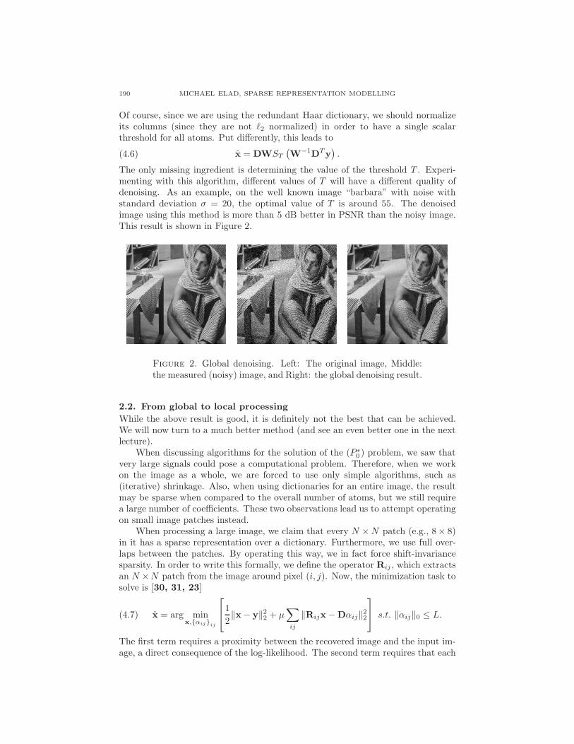
Of course, since we are using the redundant Haar dictionary, we should normalizeits columns (since they are not ℓ2 normalized) in order to have a single scalarthreshold for all atoms. Put differently, this leads to
(4.6) x = DWST
(W−1DTy
).
The only missing ingredient is determining the value of the threshold T . Experi-menting with this algorithm, different values of T will have a different quality ofdenoising. As an example, on the well known image “barbara” with noise withstandard deviation σ = 20, the optimal value of T is around 55. The denoisedimage using this method is more than 5 dB better in PSNR than the noisy image.This result is shown in Figure 2.
Figure 2. Global denoising. Left: The original image, Middle:the measured (noisy) image, and Right: the global denoising result.
2.2. From global to local processing
While the above result is good, it is definitely not the best that can be achieved.We will now turn to a much better method (and see an even better one in the nextlecture).
When discussing algorithms for the solution of the (P ǫ
0 ) problem, we saw thatvery large signals could pose a computational problem. Therefore, when we workon the image as a whole, we are forced to use only simple algorithms, such as(iterative) shrinkage. Also, when using dictionaries for an entire image, the resultmay be sparse when compared to the overall number of atoms, but we still requirea large number of coefficients. These two observations lead us to attempt operatingon small image patches instead.
When processing a large image, we claim that every N ×N patch (e.g., 8× 8)in it has a sparse representation over a dictionary. Furthermore, we use full over-laps between the patches. By operating this way, we in fact force shift-invariancesparsity. In order to write this formally, we define the operator Rij , which extractsan N ×N patch from the image around pixel (i, j). Now, the minimization task tosolve is [30, 31, 23]
(4.7) x = arg minx,{αij}ij
1
2‖x− y‖2
2 + µ∑
ij
‖Rijx − Dαij‖22
s.t. ‖αij‖0 ≤ L.
The first term requires a proximity between the recovered image and the input im-age, a direct consequence of the log-likelihood. The second term requires that each

LECTURE 4. FIRST STEPS IN IMAGE PROCESSING 191
patch in the reconstructed image can be represented well as a linear combination ofatoms from the dictionary D. The constraint forces all of these linear combinationsto be sparse.
At this stage, the dictionary we will be using for this algorithm is the over-complete DCT dictionary with 256 atoms, each representing an 8 × 8 patch. Thisdictionary is separable, allowing it so be applied efficiently.
How can we perform the minimization in (4.7)? We will take a coordinatedescent approach. First, we will fix x = y, and solve for {αij}
ij. The first term
disappears, and we are left with M · N different minimization tasks:
(4.8) αij = argminα
‖Rijx− Dα‖ s.t. ‖α‖0 ≤ L.
We have seen this problem before - this is the sparse coding problem, and can besolved by any pursuit algorithm (e.g., OMP). Once we have found {αij}
ij, we fix
them, and recover x. This is a least-squares problem and a little bit of algebraleads to a closed-form solution
(4.9) x =
I + µ
∑
ij
RT
ijRij
−1
y + µ∑
ij
RT
ijDαij
.
While this expression seems complicated, it is actually simple to implement. Whilethe operator Rij extracts a patch around the pixel (i, j), the operator RT
ijreturns
a patch to the location (i, j). Therefore, the left matrix is in fact a diagonal one,indicating for each pixel the amount of patches it belongs in, serving as normaliza-tion.
Therefore, the entire denoising process is done by extracting each patch, per-forming sparse coding, and getting a denoised patch instead. The denoised patch isreturned to its original position, with aggregation performed in the overlaps area.Then, each pixel is normalized by the number of patches it belongs too (which isgenerally N2, apart from the borders of the image).
It turns out that this very simple method performs about 2.5dB better thanthe global thresholding show previously. Furthermore, this algorithm can be im-plemented very efficiently on parallel processors. We will see this local processingapproach in several more applications. The result obtained is shown in Figure 3.
Figure 3. Local denoising. Left: The original image, Middle: themeasured (noisy) image, and Right: the local denoising result.

192 MICHAEL ELAD, SPARSE REPRESENTATION MODELLING
3. Image inpainting
Assume that a signal has been created as x = Dα0 using a very sparse vector ofcoefficients α0. Unfortunately, we do not get x directly, but rather obtain x, whichis the same signal x, but with some samples removed. We shall assume that weknow which samples are missing. Each missing sample from x implies one lostequation in the system x = Dα0. Therefore, we remove these corresponding rowsfrom the dictionary D, obtaining the dictionary D. Now, we may try to solve
(4.10) α = argminα
‖α‖0 s.t. x = Dα.
If α0 was sparse enough, it will also be the solution of this modified problem. Then,by computing Dα we will recover the original signal completely.
Using the above intuition, we now turn to extend the local denoising algorithminto an inpainting one. The minimization task here is very similar to the one wehad for the denoising (4.7), with the needed modification to take into account themasking operator [30, 31, 36],
(4.11) x = arg minx,{αij}ij
1
2‖Mx− y‖2
2 + µ∑
ij
‖Rijx − Dαij‖22
s.t. ‖αij‖0 ≤ L,
where we now require that x is close to y only in the locations of un-masked pixels.Again this minimization will be done using the coordinate descent approach.
First, we compute X = MTy (e.g., by zero filling), and do sparse coding for eachpatch, using the matching pursuit
(4.12) αij = argminα
‖Mij (Rijx − Dα) ‖ s.t. ‖α‖0 ≤ L,
with Mij the appropriate masking for each patch. Once the sparse coding is fin-ished, the result image is again reconstructed by aggregating the patches in theoverlaps area, normalizing by the number of patches in each pixel,
(4.13) x =
MT M + µ
∑
ij
RT
ijRij
−1
MT y + µ∑
ij
RT
ijDαij
.
Figure 4 presents inpainting results obtained using this algorithm.
Figure 4. Local inpainting. Left: The original image, Middle:the measured image with 50% missing pixels, and Right: the in-painting result.

LECTURE 4. FIRST STEPS IN IMAGE PROCESSING 193
4. Dictionary learning
4.1. General dictionary learning
Our entire model and applications rely on having a suitable dictionary. A gooddictionary would be one that sparsifies our data. The question we aim look at nowis how to construct such dictionaries. We have already seen one possible solution– we can choose a dictionary from an existing family of transforms, such as DCT,curvelets, contourlets, wavelets and so on. This approach has its benefits, as usuallythese transforms can be applied rather efficiently. However, a dictionary selectedthis way is typically not the best fit for the actual data.
A better approach is to train a dictionary from examples. The core idea isto collect a set of representative examples of the images we work with, and traina dictionary so that the examples can be sparsely represented over it. Such adictionary will be better suited for our data, therefore leading to better performancein various tasks.
Let us collect all the examples {xj} into a matrix X, where each column is oneexample. Then, we can write the decomposition as X ≈ DA, where each columnof A contains the coefficients for the representation of the corresponding example.A good dictionary is therefore one that is able to adequately represent each of theexamples, while the representation for each example in indeed sparse, i.e., eachcolumn in A has only a small number of non-zeros. Formally, we would like tosolve
(4.14) D, A = argminD,A
P∑
j=1
‖Dαj − xj‖ s.t. ∀j, ‖αj‖0 ≤ L.
This problem will be handled as follows: The first stage is sparse-coding, assumingD is fixed, and only the representation vectors are sought. In this stage we shouldsolve for each example
(4.15) minα
‖Dα − xj‖22 s.t. ‖α‖0 ≤ L.
We have seen in the first lecture several ways to perform this minimization, viapursuit algorithms. The second stage of dictionary training is the update of thedictionary, once the representation vectors A have been recovered. There are twomain methods to do so: the Method of Optimal Directions (MOD) method [32]and the K-SVD method [2].
4.2. MOD dictionary update
One option is to try and update the dictionary at once. The goal is minimizing
(4.16) minD
‖DA − X‖2F,
with X and A fixed. Note the use of the Frobenius norm, as both DA and X arematrices. Few simple linear algebra steps lead to
(4.17) D = XAT
(AAT
)−1= XA†.
Once the dictionary is found this way, its columns need to be re-normalized.

194 MICHAEL ELAD, SPARSE REPRESENTATION MODELLING
4.3. K-SVD dictionary learning
Another option to train the dictionary is imitating the K-means algorithm in thedictionary update stage. This means that we process one atom at a time andattempt to optimally replace it.
For processing the i-th atom, the first stage is collecting only those examplesthat use it into the matrix Xi. Then, the dictionary D and coefficient matrix A
are all fixed apart from the i-th column in D and the i-th row in A. Denotingby Di and Ai these matrices with the i-th column/row removed respectively, thefollowing residual is computed
Ei = Xi − DiAi = Xi − DA + diαi.
This is the residual matrix for all the examples that use the i-th atom, withouttaking into account the i-th atom itself. The new atom is the one that is best ableto reduce the mean residual, i.e., the result of the minimization problem
(4.18) mindi,αi
‖αidT
i− Ei‖2
F.
The vector αi is the optimal set of coefficients for this atom in each example. The
resulting atom di is inserted into the dictionary, and the new vector of coefficientsαk replaces the i-th row in A (only in the columns relevant to the examples usingthis atom).
The optimization task in (4.18) is in fact a rank-1 approximation, which canbe solved directly using the SVD decomposition. As every atom is updated usingan SVD operation, this algorithm is appropriately named K-SVD. Note, that inthe MOD training stage, the matrix of coefficients A is held constant, and thedictionary D is adapted to it. In the K-SVD algorithm, on the other hand, theatom update stage also optimizes for the k’th row of A at the same time.
LECTURE 5
Image processing - more practice
In the previous lecture we saw how to denoise and inpaint an image based onlocal, patch-processing. However, in both this cases, we used a fixed dictionary – thelocal DCT. In this lecture we shall revisit these two applications, and incorporateinto them the K-SVD, in an attempt to improve their performance. We shall alsodemonstrate the capabilities of the Sparseland model in handling image processingtasks by considering two new applications – an image scale-up process based on apair of trained dictionaries, and a facial image compression algorithm that performsbetter than JPEG-2000. More details on the applications presented here can befound in [22, 3].
1. Image denoising with a learned dictionary
When thinking about dictionary learning, both the MOD and the K-SVD are notable to process signals with large dimensions. The reason is obvious – a high dimen-sional signal implies a dictionary held as a very large explicit matrix, intolerableamounts of computations, both for the training and for using this dictionary, anda huge amount of examples to learn from, in order to avoid over-fitting. Thus,learned dictionaries are naturally used for low-dimensional signals.
We have already seen in the previous lecture that denoising (and inpainting)can be done very effectively by operating on small (e.g., 8 × 8) patches. Theprocessing is then done on local blocks of images, using a dictionary that handleslow-dimensional signals. Formally, the denoising we have proposed is written as
(5.1) x = arg minx,{αij}ij
1
2‖x− y‖2
2 + µ∑
ij
‖Rijx − Dαij‖22
s.t. ‖αij‖0 ≤ L.
The second term is the prior, expressing our belief that every patch in the imageshould have a sparse representation over the dictionary D. Our objective is tointroduce a learned dictionary into the above paradigm. One option is collecting aset of high-quality images, extract patches from them, and use these examples totrain a dictionary. This dictionary will be a “universal dictionary”, as it is trainedon general content images. This option is useful, and brings reasonably good results- about 0.5-1dB below the state of the art.
An interesting alternative is to use patches from the corrupted image itself forthe training process. Suppose an image of 1000 × 1000 is to be denoised. Such animage contains nearly 106 patches, which are more than enough to allow trainingthe dictionary. Furthermore, since the dictionary training process contains somesort of averaging, the resulting dictionary will actually be (almost) noise free, andcan thus be used for denoising.
195

196 MICHAEL ELAD, SPARSE REPRESENTATION MODELLING
This option works much better than using the “universal dictionary”, and leadsto state-of-the-art results [23]. In fact, going back to the penalty term in (5.1), wecan bring about this option by minimizing over D as well. Again, a coordinatedescent approach is used. First, the image x = y is fixed, and the dictionaryD is fixed on some initialization (e.g., the redundant DCT). Each patch in theimage undergoes sparse coding. Freezing the representations, the dictionary isupdated. All the patches then undergo sparse coding with the new dictionary, andso. Iterating several times between sparse coding and dictionary update is exactlythe training procedure we have seen in the previous lecture, performed over thepatches in the image. After several such training iterations, the final dictionaryis used for one last sparse-coding stage. Then, the sparse representations andthe dictionary are fixed, and the result image is recovered, using the same simpleaggregation method shown in the previous lecture,
(5.2) x =
I + µ
∑
ij
RT
ijRij
−1
y + µ∑
ij
RT
ijDαij
.
Figure 1 presents the result obtained using this algorithm, for the same test shown inLecture 4. The obtained image has PSNR = 31dB, which is 1dB higher comparedto the DCT-based outcome.
Figure 1. Local denoising with a trained dictionary. Left: Theoriginal image, Middle: the noisy image (σ = 20), and Right: thedenoising result.
This denoising algorithm has been applied to many variation of the denoisingproblem. One is of course the denoising of gray-scale images. When published, thismethod led to state-of-the-art results. Later, it was extended by Mairal et. al. byusing joint sparsity (i.e., sparse coding similar patches together) [37]. This methodis currently the best performing denoising algorithm.
The denoising algorithm could also be applied to denoising of color images.Usually, there is a sensitivity in how the relationships between the color channelsshould be handled. In this algorithm, the solution is simple – the training is per-formed on 8×8×3 patches, i.e., on colored patches extracted from the image. Thedictionary contains color atoms, and the rest of the algorithm remains the same.This method is also the state-of-the-art in color image denoising [36].
Video sequences can also be handled by this method. When processing imagesequences, the redundancy between frames can and should be used in order toachieve better denoising. While most video denoising algorithms require motion

LECTURE 5. IMAGE PROCESSING - MORE PRACTICE 197
estimation (which is error-prone), the suggested method can simply train on space-time patches extracted from the video. Therefore, the dictionary is also constructedof “movielets”, as each atom is a very short, very small (e.g., 8× 8× 5) space-timepatch. Furthermore, since consecutive images are very similar, it is not necessaryto retrain a dictionary for each image. Instead, it can be propagated from oneframe to the next, only requiring fine tuning (1 K-SVD iteration) for each one.This method’s performance is equivalent to the state-of-the-art [43].
2. Image inpainting with dictionary learning
Turning to image inpainting, we would like to apply dictionary learning here aswell, for handling the local patches. The process is very similar to the one donein denoising. The algorithm starts with dictionary training using the K-SVD, byperforming alternating steps between sparse coding and dictionary update. Duringthe sparse coding stage, only the un-masked (i.e., known) pixels in each patchare used. This is similar to the sparse coding undertaken in the fixed dictionaryscenario. Once the sparse coding is done, each atom is updated using the SVDoperation, just like the K-SVD method.
This dictionary training is repeated for several (e.g., 10) iterations. Then, theimage is reconstructed from the final sparse coding using the same formula we haveseen:
(5.3) x = arg minx,{αij}ij
1
2‖Mx− y‖2
2 + µ∑
ij
‖Rijx − Dαij‖22
s.t. ‖αij‖0 ≤ L,
Of course, just like in the denoising case, this method can be easily generalizedto inpainting of color images and inpainting of video sequences using the sameextensions as in the denoising case. Figure 2 presents the results obtained with thisalgorithm, showing the benefit of using learned dictionary.
This approach to inpainting works well when the missing pixels are in (near-random) locations, or organized in small groups. If the missing pixels form a largearea to reconstruct, the local approach will not work, and an alternative, global,approach will be needed.
Another problem could arise if the missing pixels create a periodic mask, forexample, when every other pixel is missing. In this case, the dictionary will notbe able to learn the relationship between neighboring pixels, because it has noinformation about such neighbors. Such is the case, for example, in image single-image scale-up and demosaicing. The periodic nature of the mask pattern may causethe learned dictionary to absorb this pattern into its atoms. In order to preventthat, the dictionary should trained while allowing only a very small number of non-zeros, and furthermore, only few training iterations in order to avoid over-fitting.Such a solution leads to state of the art results, which can be seen in [36].
3. Image scale-up with a pair of dictionaries
We turn to describe an image scale-up algorithm that uses trained dictionaries.The method described here follows the work of Yang et. al. [54], with severalimportant modifications that lead to a simpler and more efficient algorithm, withbetter results [22].

198 MICHAEL ELAD, SPARSE REPRESENTATION MODELLING
Figure 2. Image inpainting with the K-SVD. Top-Left: The orig-inal image, Top-Right: the measured image (masked with missingpixels), Bottom Left: DCT-based inpainting, and Bottom Right:the proposed K-SVD inpainting result.
3.1. Preliminaries
The image scale-up problem is defined as follows. A high-quality (high-resolution)image yh is blurred, decimated, and contaminated by additive noise, obtaining theimage zl,
(5.4) zl = SHyl + v,
with H a blur operation, S the decimation operator, and v the noise. We assumethat the decimation S and blur H operators, and the statistical properties of thenoise v, are known.
We would like to reverse this process and recover the high quality image fromthe given low quality one. This is a severely ill-posed inverse problem, and thereforewe shall need an image model for its regularization – we shall use the Sparselandmodel.
In order to simplify notations, we will assume the the low resolution imagehas undergone simple interpolation (such as bicubic) to the same size as the targetimage
(5.5) yl = Qzl,

LECTURE 5. IMAGE PROCESSING - MORE PRACTICE 199
with Q being the interpolation operator. This initialization step will save us thetechnicalities of handling two scales in our formulation.
The algorithm we suggest relies on two core ideas. The first is operating locally,in the sense that each patch in the low-quality image will undergo resolution en-hancement on its own. Then, the improved patches will be merged (using averagingin the overlap areas, just as in the previously described denoising and inpainting)in order to create the final output image.
How each patch is enhanced? This enhancement requires two dictionaries, Al
and Ah for the low and high quality patches respectively. Each atom in Ah shouldbe the high-quality counterpart of the corresponding low quality atom in Al. Inorder to enhance a low-quality patch, its sparse representation over the low-qualitydictionary Al is found. This sparse representation is then used to reconstruct apatch from the high-quality dictionary, which is the enhancement result for thelow-quality patch. We will now go into further details of this algorithm, and focuson learning these two dictionaries.
3.2. The core idea
As we have been practicing throughout this course, we assume that every√
n×√n
patch extracted from location k in the high-quality image through pk
h= Rkyh,
can be represented sparsely over a high-quality dictionary Ah, i.e., for every patchpk
hwe assume that there exists a very sparse representation vector qk such that
pk
h
∼= Ahqk.
Next, we aim to find a connection between a high-quality patch in yh and apatch in the same location in yl. We can use our knowledge of the creation processof zl from yh through blur, decimation and the addition of noise, with interpolationused to create yl. Therefore,
(5.6) yl = Q (DHyh + v) .
Combining all operators into one LALL = QDH, we come to the relationship foreach patch
(5.7) ‖Lpk
h− pk
l‖2 ≤ ǫ,
with L a local portion of LALL. This expression ties the low-quality patch and thehigh-quality patch in the same location. Using our assumption that the high qualitypatch can be sparsely represented over the high quality dictionary pk
h
∼= Ahqk, we
obtain the relationship ‖LAhqk −pk
l‖2 ≤ ǫ. Defining a new dictionary, Al = LAh,
we obtain
(5.8) ‖Alqk − pk
l‖2 ≤ ǫ.
This observation leads to the conclusion that the sparse representation qk is alsothe representation of the low quality patch pk
lover the low quality dictionary Al.
3.3. Dictionary training
Since we want to use trained dictionaries, the obvious question is what do we trainthem on. One option is obtaining one (or more) high quality images. The high-quality image is then blurred and down-sampled it using the known (expected)operators. The low-resolution image is then interpolated back to the size of thehigh-quality image. Then, all the patches from each image are extracted, withpatches in the same location in the original and interpolated image being paired.
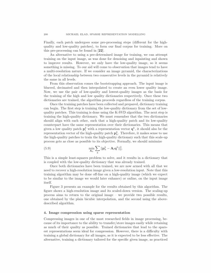
200 MICHAEL ELAD, SPARSE REPRESENTATION MODELLING
Finally, each patch undergoes some pre-processing steps (different for the high-quality and low-quality patches), to form our final corpus for training. More onthis pre-processing can be found in [22].
An alternative to using a pre-determined image for training, we can attempttraining on the input image, as was done for denoising and inpainting and shownto improve results. However, we only have the low-quality image, so it seemssomething is missing. To our aid will come to observation that images tend to havea multi-resolution nature. If we consider an image pyramid, the characterizationsof the local relationship between two consecutive levels in the pyramid is relativelythe same in all levels.
From this observation comes the bootstrapping approach. The input image isblurred, decimated and then interpolated to create an even lower quality image.Now, we use the pair of low-quality and lowest-quality images as the basis forthe training of the high and low quality dictionaries respectively. Once these twodictionaries are trained, the algorithm proceeds regardless of the training corpus.
Once the training patches have been collected and prepared, dictionary trainingcan begin. The first step is training the low-quality dictionary from the set of low-quality patches. This training is done using the K-SVD algorithm. The next step istraining the high-quality dictionary. We must remember that the two dictionariesshould align with each other, such that a high-quality patch and its low-qualitycounterpart have the same representation over their dictionaries. This means thatgiven a low quality patch pk
lwith a representation vector qk, it should also be the
representation vector of the high-quality patch pk
h. Therefore, it makes sense to use
the high-quality patches to train the high-quality dictionary such that this scale-upprocess gets as close as possible to its objective. Formally, we should minimize
(5.9) minAh
∑
k
‖pk
h− Alq
k‖22.
This is a simple least-squares problem to solve, and it results in a dictionary thatis coupled with the low-quality dictionary that was already trained.
Once both dictionaries have been trained, we are now armed with all that weneed to recover a high-resolution image given a low-resolution input. Note that thistraining algorithm may be done off-line on a high-quality image (which we expectto be similar to the image we would later enhance) or online, on the input imageitself.
Figure 3 presents an example for the results obtained by this algorithm. Thefigure shows a high-resolution image and its scaled-down version. The scaling-upprocess aims to return to the original image – we provide two possible results,one obtained by the plain bicubic interpolation, and the second using the above-described algorithm.
4. Image compression using sparse representation
Compressing images in one of the most researched fields in image processing, be-cause of its importance to the ability to transfer/store images easily while retainingas much of their quality as possible. Trained dictionaries that lead to the spars-est representations seem ideal for compression. However, there is a difficulty withtraining a global dictionary for all images, as it is expected to be less effective. Thealternative, training a dictionary tailored for the specific given image, as practiced

LECTURE 5. IMAGE PROCESSING - MORE PRACTICE 201
Figure 3. Image Scale-Up. Top-Left: The original image, Top-Right: the measured image (blurred, decimated, and noisy), Bot-tom Left: Bicubic scaled-up image, and Bottom Right: the pro-posed scale-up result.
in denoising and inpainting, is also difficult, as it requires allocated bits for thedictionary, which may compromise the success of the compression algorithm.
When turning to a specific family of images, the story changes, as it is nowpossible to tailor specific dictionaries to the task, while not actually needing tosend them. One example for such a problem is the compression of high-quality(e.g., 500 × 400) facial ID images, to put on biometric identity cards or creditcards. It is possible to use general purpose compression algorithms, such as JPEGand JPEG2000 for this purpose, but a specifically trained algorithm is expected todo much better.
The proposed algorithm we describe here [4] has two stages – first, trainingappropriate dictionaries, and then, applying the trained dictionaries to compress(and decompress) the facial images.
4.1. Facial image compression algorithm - training
For training, a set of high-quality facial images are collected. This set is then usedfor training a dictionary for each portion of the image. The stages are as following:

202 MICHAEL ELAD, SPARSE REPRESENTATION MODELLING
(1) Key points in each image are detected (e.g., eyes, nose). These locationsare used to transform each image (using a piece-wise affine transform) suchthat these key points are in exactly the same coordinates in all images.
(2) Each image is divided into non-overlapping 15× 15 patches. Overlaps areavoided as redundancy will only worsen the compression rate.
(3) All patches in the same location are collected into a set.(4) The mean of each set of patches is computed, stored, and removed from
each patch.(5) For each set, a dictionary is trained, either using a linear approximation
(i.e., PCA) or non-linear approximation (i.e., K-SVD).(6) Each patch location is assigned a constant number of atoms to use, and
quantization levels to use, both varying from location to location. Thisassignment is done by minimizing the mean error on the training set whileachieving the desired compression rate.
Once the training procedure ends, for each patch location, its mean patch,dictionary, number of allotted atoms and quantization levels are stored both in theencoder and decoder.
4.2. Compressing and decompressing
When a new image is to be compressed, it undergoes the following stages (similarto the training stage):
(1) The same key points in the image are detected and the image is warped.(2) The (warped) image is divided into non-overlapping 15× 15 patches.(3) For each patch, the mean of this location is removed.(4) Sparse coding over this location’s dictionary (or projection onto the PCA)
is carried out, using the number of atoms allotted to this location.(5) The values of the coefficients selected are quantized.(6) Entropy coding is used to further compress the sent values.
Note that if K-SVD is used, when sending the atoms’ coefficients their indicesare sent as well, while in PCA, only the coefficients are sent. The recovery algorithmis the exact opposite. Entropy de-coding is performed on the sent data, and eachpatch is then reconstructed from the send coefficients (and indices if K-SVD isused). The inverse transform is applied to the image, returning to an image that isas close as possible to the original. Figure 4 presents the obtained results for 550Bytes per image.
5. Summary
The field of sparse and redundant representation modeling offers a new model, andthis can be brought to various problems in image processing, often leading to state-of-the-art results. We have seen in these lecture-notes a partial list of these successstories, and many more have been introduced to the scientific community in thepast few years. More applications, and more details in general about this field andits impact to image processing, can be found in my book:
M. Elad, Sparse and Redundant Representations:From Theory to Applications in Signal and ImageProcessing, Springer, New-York, 2010.

LECTURE 5. IMAGE PROCESSING - MORE PRACTICE 203
Figure 4. Facial image compression. From left to right: the orig-inal image, JPEG results, JPEG-2000 results, local-PCA, and K-SVD. The numbers represent the mean-squared-error per pixel af-ter compression and decompression with 550 Bytes.


Bibliography
[1] Z. Ben-Haim, Y.C. Eldar, and M. Elad, Coherence-based performance guarantees
for estimating a sparse vector under random noise, to appear in IEEE Trans. onSignal Processing.
[2] M. Aharon, M. Elad, and A.M. Bruckstein. K-SVD: An algorithm for designing of
overcomplete dictionaries for sparse representation, IEEE Trans. on Signal Pro-cessing, 54(11):4311–4322, November 2006.
[3] A.M. Bruckstein, D. L. Donoho, and M. Elad, From sparse solutions of systems
of equations to sparse modeling of signals and images, SIAM Review, 51(1):34-81,
2009.
[4] O. Bryt and M. Elad, Compression of facial images using the K-SVD algorithm,
Journal of Visual Communication and Image Representation, 19(4):270–283, May
2008.
[5] E.J. Candes, J. Romberg, and T. Tao, Robust uncertainty principles: Exact signal
reconstruction from highly incomplete frequency information, IEEE Trans. Inform.Theory, 52:489-509, 2006.
[6] E.J. Candes and T. Tao, The Dantzig selector: Statistical estimation when p is
much larger than n, Annals of Statistics, 35(6):2313–2351, June 2007.
[7] S.S. Chen, D.L. Donoho, and M.A. Saunders, Atomic decomposition by basis pur-
suit, SIAM Journal on Scientific Computing, 20(1):33–61 (1998).
[8] I. Daubechies, M. Defrise, and C. De-Mol, An iterative thresholding algorithm for
linear inverse problems with a sparsity constraint, Communications on Pure andApplied Mathematics, LVII:1413–1457, 2004.
[9] G. Davis, S. Mallat, and M. Avellaneda, Adaptive greedy approximations, Journalof Constructive Approximation, 13:57–98, 1997.
[10] M.N. Do and M. Vetterli, The contourlet transform: an efficient directional
multiresolution image representation, IEEE Trans. Image on Image Processing,14(12):2091–2106, 2005.
[11] D.L. Donoho, De-noising by soft thresholding, IEEE Trans. on Information The-ory, 41(3):613–627, 1995.
[12] D.L. Donoho, For most large underdetermined systems of linear equations, the
minimal ℓ1-norm solution is also the sparsest solution, Communications On PureAnd Applied Mathematics, 59(6):797–829, June 2006.
[13] D.L. Donoho, For most large underdetermined systems of linear equations, the
minimal ℓ1-norm near-solution approximates the sparsest near-solution, Commu-nications On Pure And Applied Mathematics, 59(7):907–934, July 2006.
[14] D.L. Donoho and M. Elad, Optimally sparse representation in general (non-
orthogonal) dictionaries via l1 minimization, Proc. of the National Academy ofSciences, 100(5):2197–2202, 2003.
[15] D.L. Donoho and M. Elad, On the stability of the basis pursuit in the presence of
noise, Signal Processing, 86(3):511–532, March 2006.
[16] D.L. Donoho, M. Elad, and V. Temlyakov, Stable recovery of sparse overcomplete
representations in the presence of noise, IEEE Trans. On Information Theory,52(1):6–18, 2006.
[17] D.L. Donoho and I.M. Johnstone, Ideal denoising in an orthonormal basis chosen
from a library of bases, Comptes Rendus del’Academie des Sciences, Series A,
319:1317–1322, 1994.
205

206 MICHAEL ELAD, SPARSE REPRESENTATION MODELLING
[18] D.L. Donoho and J. Tanner, Neighborliness of randomly-projected Simplices in
high dimensions, Proceedings Of The National Academy Of Sciences, 102(27):9452–
9457, July 2005.
[19] D.L. Donoho and J. Tanner, Sparse nonnegative solutions of underdetermined lin-
ear equations by linear programming, Proc. Natl. Acad. Sci., 102:9446-9451 , 2005.
[20] B. Efron, T. Hastie, I.M. Johnstone, and R. Tibshirani, Least angle regression, TheAnnals of Statistics, 32(2):407–499, 2004.
[21] M. Elad, Why simple shrinkage is still relevant for redundant representations?, to
appear in the IEEE Trans. On Information Theory.[22] M. Elad, Sparse and Redundant Representations: From Theory to Applications in
Signal and Image Processing, Springer New-York, 2010.
[23] M. Elad and M. Aharon, Image denoising via sparse and redundant representations
over learned dictionaries, IEEE Trans. on Image Processing 15(12):3736–3745, De-
cember 2006.
[24] M. Elad, B. Matalon, and M. Zibulevsky, Coordinate and subspace optimization
methods for linear least squares with non-quadratic regularization, Applied andComputational Harmonic Analysis, 23:346–367, November 2007.
[25] M. Elad and M. Zibulevsky, Iterative shrinkage algorithms and their acceleration for
l1-l2 signal and image processing applications”, IEEE Signal Processing Magazine,
27(3):78–88, May 2010.
[26] M.A. Figueiredo and R.D. Nowak, An EM algorithm for wavelet-based image
restoration, IEEE Trans. Image Processing, 12(8):906–916, 2003.
[27] M.A. Figueiredo, and R.D. Nowak, A bound optimization approach to wavelet-
based image deconvolution, IEEE International Conference on Image Processing -
ICIP 2005, Genoa, Italy, 2:782–785, September 2005.
[28] I.F. Gorodnitsky and B.D. Rao, Sparse signal reconstruction from limited data
using FOCUSS: A re-weighted norm minimization algorithm, IEEE Trans. OnSignal Processing, 45(3):600–616, 1997.
[29] R. Gribonval and M. Nielsen, Sparse decompositions in unions of bases, IEEETrans. on Information Theory, 49(12):3320–3325, 2003.
[30] O.G. Guleryuz, Nonlinear approximation based image recovery using adaptive
sparse reconstructions and iterated denoising - Part I: Theory, IEEE Trans. onImage Processing, 15(3):539–554, 2006.
[31] O.G. Guleryuz, Nonlinear approximation based image recovery using adaptive
sparse reconstructions and iterated denoising - Part II: Adaptive algorithms, IEEETrans. on Image Processing, 15(3):555–571, 2006.
[32] K. Kreutz-Delgado, J.F. Murray, B.D. Rao, K. Engan, T-W, Lee, and T.J. Se-
jnowski, Dictionary learning algorithms for sparse representation, Neural Compu-tation, 15(2)349–396, 2003.
[33] S.-J. Kim, K. Koh, M. Lustig, S. Boyd, and D. Gorinevsky, A method for large-
scale ,1-regularized least squares problems with applications in signal processing
and statistics, IEEE J. Selected Topics Signal Processing, 1(4):606-617, Dec. 2007.
[34] J.B. Kruskal, Three-way arrays: rank and uniqueness of trilinear decompositions,
with application to arithmetic complexity and statistics, Linear Algebra and itsApplications, 18(2):95–138, 1977.
[35] X. Liu and N.D. Sidiropoulos, Cramer-Rao lower bounds for low-rank decompo-
sition of multidimensional arrays, IEEE Trans. on Signal Processing, 49(9):2074–
2086, 2001.
[36] J. Mairal, M. Elad, and G. Sapiro, Sparse representation for color image restoration,
IEEE Trans. on Image Processing, 17(1):53–69, January 2008.
[37] J. Mairal, F. Bach, J. Ponce, G. Sapiro and A. Zisserman, Non-local sparse mod-
els for image restoration, International Conference on Computer Vision (ICCV),
Tokyo, Japan, 2009.
[38] S. Mallat, A Wavelet Tour of Signal Processing, Academic-Press, Second-Edition,
2009.
[39] S. Mallat and E. LePennec, Sparse geometric image representation with bandelets,
IEEE Trans. on Image Processing, 14(4):423–438, 2005.

207 BIBLIOGRAPHY
[40] S. Mallat and Z. Zhang, Matching pursuits with time-frequency dictionaries, IEEETrans. Signal Processing, 41(12):3397–3415, 1993.
[41] B.K. Natarajan, Sparse approximate solutions to linear systems, SIAM Journal onComputing, 24:227–234, 1995.
[42] Y.C. Pati, R. Rezaiifar, and P.S. Krishnaprasad, Orthogonal matching pursuit:
recursive function approximation with applications to wavelet decomposition, the
twenty seventh Asilomar Conference on Signals, Systems and Computers, 1:40–44,
1993.
[43] M. Protter and Michael Elad, Image sequence denoising via sparse and redundant
representations, IEEE Trans. on Image Processing, 18(1):27–36, January 2009.
[44] L. Rudin, S. Osher, and E. Fatemi, Nonlinear total variation based noise removal
algorithms, Physica D, 60:259–268, 1992
[45] E.P. Simoncelli, W.T. Freeman, E.H. Adelsom, and D.J. Heeger, Shiftable multi-
scale transforms, IEEE Trans. on Information Theory, 38(2):587–607, 1992.
[46] J.-L. Starck, E.J. Candes, and D.L. Donoho, The curvelet transform for image
denoising, IEEE Trans. on Image Processing, 11:670–684, 2002.
[47] J.-L. Starck, M. Elad, and D.L. Donoho, Redundant multiscale transforms and
their application for morphological component separation, Advances in ImagingAnd Electron Physics, 132:287–348, 2004.
[48] J.-L. Starck, M. Elad, and D.L. Donoho, Image decomposition via the combina-
tion of sparse representations and a variational approach. IEEE Trans. On ImageProcessing, 14(10):1570–1582, 2005.
[49] T. Strohmer and R. W. Heath, Grassmannian frames with applications to coding
and communication, Applied and Computational Harmonic Analysis, 14:257–275,
2004.
[50] J.A. Tropp, Greed is good: Algorithmic results for sparse approximation, IEEETrans. On Information Theory, 50(10):2231–2242, October 2004.
[51] J.A. Tropp, Just relax: Convex programming methods for subset selection and
sparse approximation, IEEE Trans. On Information Theory, 52(3):1030–1051,
March 2006.
[52] J.A. Tropp, I.S. Dhillon, R.W. Heath Jr., and T. Strohmer, Designing struc-
tured tight frames via alternating projection, IEEE Trans. Information Theory,51(1):188–209, January 2005.
[53] J.A. Tropp and A.A. Gilbert, Signal recovery from random measurements via or-
thogonal matching pursuit, Submitted for publication, April 2005.
[54] J. Yang, J. Wright, T. Huang, and Y. Ma, Image super-resolution via sparse rep-
resentation, to appear in PIEEE Trans. on Image Processing.
