lecturer: mcgreevy these lecture notes livehere. please...
TRANSCRIPT
Physics 215C: Particles and Fields
Spring 2017
Lecturer: McGreevy
These lecture notes live here. Please email corrections to mcgreevy at physics dot
ucsd dot edu.
Last updated: 2018/10/11, 17:37:18
1
Contents
0.1 Introductory remarks for the third quarter . . . . . . . . . . . . . . . . 3
0.2 Sources . . . . . . . . . . . . . . . . . . . . . . . . . . . . . . . . . . . . 6
0.3 Conventions . . . . . . . . . . . . . . . . . . . . . . . . . . . . . . . . . 8
11 Resolving the identity 9
11.1 Quantum-classical correspondence . . . . . . . . . . . . . . . . . . . . . 9
11.2 Interlude on differential forms and algebraic topology . . . . . . . . . . 24
11.3 Coherent state path integrals for spin systems . . . . . . . . . . . . . . 27
11.4 Coherent state path integrals for fermions . . . . . . . . . . . . . . . . 53
11.5 Coherent state path integrals for bosons . . . . . . . . . . . . . . . . . 61
12 Anomalies 68
13 Saddle points, non-perturbative field theory and resummations 79
13.1 Instantons in the Abelian Higgs model in D = 1 + 1 . . . . . . . . . . . 79
13.2 Blobology (aka Large Deviation Theory) . . . . . . . . . . . . . . . . . 83
13.3 Coleman-Weinberg potential . . . . . . . . . . . . . . . . . . . . . . . . 96
14 Duality 109
14.1 XY transition from superfluid to Mott insulator, and T-duality . . . . . 109
14.2 (2+1)-d XY is dual to (2+1)d electrodynamics . . . . . . . . . . . . . . 119
14.3 Deconfined Quantum Criticality . . . . . . . . . . . . . . . . . . . . . . 132
15 Effective field theory 139
15.1 Fermi theory of Weak Interactions . . . . . . . . . . . . . . . . . . . . . 142
15.2 Loops in EFT . . . . . . . . . . . . . . . . . . . . . . . . . . . . . . . . 143
15.3 The Standard Model as an EFT. . . . . . . . . . . . . . . . . . . . . . 149
15.4 Pions . . . . . . . . . . . . . . . . . . . . . . . . . . . . . . . . . . . . . 152
15.5 Quantum Rayleigh scattering . . . . . . . . . . . . . . . . . . . . . . . 158
15.6 Superconductors . . . . . . . . . . . . . . . . . . . . . . . . . . . . . . 160
15.7 Effective field theory of Fermi surfaces . . . . . . . . . . . . . . . . . . 164
2
0.1 Introductory remarks for the third quarter
Last quarter, we grappled with the Wilsonian perspective on the RG, which (among
many other victories) provides an explanation of the totalitarian principle of physics,
that anything that can happen must happen. More precisely, this means that the
Hamiltonian should contain all terms consistent with symmetries, organized according
to an expansion in decreasing relevance to low energy physics.
This leads directly to the idea of effective field theory, or, how to do physics without
a theory of everything. (You may notice that all the physics that has been done has
been done without a theory of everything.) It is a weaponized version of selective
inattention.
So here are some goals, both practical and philosophical:
• We’ll continue our study of coarse-graining in quantum systems with extensive
degrees of freedom, aka the RG in QFT.
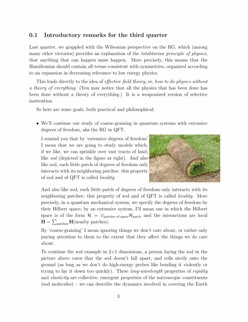
I remind you that by ‘extensive degrees of freedom’
I mean that we are going to study models which,
if we like, we can sprinkle over vast tracts of land,
like sod (depicted in the figure at right). And also
like sod, each little patch of degrees of freedom only
interacts with its neighboring patches: this property
of sod and of QFT is called locality.
And also like sod, each little patch of degrees of freedom only interacts with its
neighboring patches: this property of sod and of QFT is called locality. More
precisely, in a quantum mechanical system, we specify the degrees of freedom by
their Hilbert space; by an extensive system, I’ll mean one in which the Hilbert
space is of the form H = ⊗patches of spaceHpatch and the interactions are local
H =∑
patches H(nearby patches).
By ‘coarse-graining’ I mean ignoring things we don’t care about, or rather only
paying attention to them to the extent that they affect the things we do care
about.
To continue the sod example in 2+1 dimensions, a person laying the sod in the
picture above cares that the sod doesn’t fall apart, and rolls nicely onto the
ground (as long as we don’t do high-energy probes like bending it violently or
trying to lay it down too quickly). These long-wavelength properties of rigidity
and elasticity are collective, emergent properties of the microscopic constituents
(sod molecules) – we can describe the dynamics involved in covering the Earth
3
with sod (never mind whether this is a good idea in a desert climate) without
knowing the microscopic theory of the sod molecules (‘grass’). Our job is to think
about the relationship between the microscopic model (grassodynamics) and its
macroscopic counterpart (in this case, suburban landscaping). In my experience,
learning to do this is approximately synonymous with understanding.
• I would like to convince you that “non-renormalizable” does not mean “not worth
your attention,” and explain the incredibly useful notion of an Effective Field
Theory.
• There is more to QFT than perturbation theory about free fields in a Fock vac-
uum. In particular, we will spend some time thinking about non-perturbative
physics, effects of topology, solitons. Topology is one tool for making precise
statements without perturbation theory (the basic idea: if we know something is
an integer, it is easy to get many digits of precision!).
• I will try to resist making too many comments on the particle-physics-centric
nature of the QFT curriculum, since the curriculum this year has been largely
up to me. (In previous years when I’ve taught 215C, other folks taught 215A
and 215B, but this time I have no one but myself to blame for misinforming you
about how to think about quantum fields.) But I want to emphasize that QFT
is also quite central in many aspects of condensed matter physics, and we will
learn about this. From the point of view of someone interested in QFT, high
energy particle physics has the severe drawback that it offers only one example!
(OK, for some purposes we can think about QCD and the electroweak theory
separately...)
From the high-energy physics point of view, we could call this the study of reg-
ulated QFT, with a particular kind of lattice regulator. Why make a big deal
about ‘regulated’? Besides the fact that this is how QFT comes to us (when it
does) in condensed matter physics, such a description is required if we want to
know what we’re talking about. For example, we need it if we want to know
what we’re talking about well enough to explain it to a computer. Many QFT
problems are too hard for our brains. A related but less precise point is that I
would like to do what I can to erase the problematic perspective on QFT which
‘begins from a classical lagrangian and quantizes it’ etc, and leads to a term like
‘anomaly’. (We will talk about what is ‘anomaly’ this quarter.)
• There is more to QFT than the S-matrix. In a particle-physics QFT course (like
this year’s 215A!) you learn that the purpose in life of correlation functions or
green’s functions or off-shell amplitudes is that they have poles (at pµpµ−m2 = 0)
4
whose residues are the S-matrix elements, which are what you measure (or better,
are the distribution you sample) when you scatter the particles which are the
quanta of the fields of the QFT. I want to make two extended points about this:
1. In many physical contexts where QFT is relevant, you can actually measure
the off-shell stuff. This is yet another reason why including condensed matter
in our field of view will deepen our understanding of QFT.
2. This is good, because the Green’s functions don’t always have simple poles!
There are lots of interesting field theories where the Green’s functions in-
stead have power-law singularities, like G(p) ∼ 1p2∆ . If you Fourier trans-
form this, you don’t get an exponentially-localized packet. The elementary
excitations created by a field whose two point function does this are not
particles. (Any conformal field theory (CFT) is an example of this.) The
theory of particles (and their dance of creation and annihilation and so on)
is an important but proper subset of QFT.
• The crux of many problems in physics is the correct choice of variables with
which to label the degrees of freedom. Often the best choice is very different
from the obvious choice; a name for this phenomenon is ‘duality’. We will study
many examples of it (Kramers-Wannier, Jordan-Wigner, bosonization, Wegner,
particle-vortex, perhaps others). This word is dangerous (at one point it was one
of the forbidden words on my blackboard) because it is about ambiguities in our
(physics) language. I would like to reclaim it.
An important bias in deciding what is meant by ‘correct’ or ‘best’ in the previous
paragraph is: we will be interested in low-energy and long-wavelength physics,
near the groundstate. For one thing, this is the aspect of the present subject which
is like ‘elementary particle physics’; the high-energy physics of these systems is
of a very different nature and bears little resemblance to the field often called
‘high-energy physics’ (for example, there is volume-law entanglement).
• We’ll be interested in models with a finite number of degrees of freedom per
unit volume. This last is important, because we are going to be interested in the
thermodynamic limit. Questions about a finite amount of stuff (this is sometimes
called ‘mesoscopics’) tend to be much harder.
• An important goal for the course is demonstrating that many fancy phenomena
precious to particle physicists can emerge from very humble origins in the kinds of
(completely well-defined) local quantum lattice models we will study. Here I have
in mind: fermions, gauge theory, photons, anyons, strings, topological solitons,
CFT, and many other sources of wonder I’m forgetting right now.
5
Here is a confession, related to several of the points above: The following comment
in the book Advanced Quantum Mechanics by Sakurai had a big effect on my education
in physics: ... we see a number of sophisticated, yet uneducated, theoreticians who
are conversant in the LSZ formalism of the Heisenberg field operators, but do not know
why an excited atom radiates, or are ignorant of the quantum-theoretic derivation of
Rayleigh’s law that accounts for the blueness of the sky. I read this comment during
my first year of graduate school and it could not have applied more aptly to me. I
have been trying to correct the defects in my own education which this exemplifies ever
since. I bet most of you know more about the color of the sky than I did when I was
your age, but we will come back to this question. (If necessary, we will also come back
to the radiation from excited atoms.)
So I intend that there will be two themes of this course: coarse-graining and topol-
ogy. Both of these concepts are important in both hep-th and in cond-mat. Topics
which I hope to discuss include:
• the uses and limitations of path integrals of various kinds
• some illustrations of effective field theory (perhaps cleverly mixed in with the
other subjects)
• effects of topology in QFT (this includes anomalies, topological solitons and
defects, topological terms in the action)
• more deep mysteries of gauge theory and its emergence in physical systems.
• If there is demand for it, we will discuss non-abelian gauge theory, in perturbation
theory: Fadeev-Popov ghosts, and the sign of the Yang-Mills beta function. Sim-
ilarly, we can talk about other topics relevant to the Standard Model of particle
physics if there is demand.
• Large-N expansions?
• duality.
I welcome your suggestions regarding which subjects in QFT we should study.
0.2 Sources
The material in these notes is collected from many places, among which I should
mention in particular the following:
Peskin and Schroeder, An introduction to quantum field theory (Wiley)
6
Zee, Quantum Field Theory (Princeton, 2d Edition)
Banks, Modern Quantum Field Theory: A Concise Introduction (Cambridge)
Schwartz, Quantum field theory and the standard model (Cambridge)
Coleman, Aspects of Symmetry (Cambridge)
Polyakov, Gauge Field and Strings (Harwood)
Wen, Quantum field theory of many-body systems (Oxford)
Sachdev, Quantum Phase Transitions (Cambridge, 2d Edition)
Many other bits of wisdom come from the Berkeley QFT courses of Prof. L. Hall
and Prof. M. Halpern.
7
0.3 Conventions
Following most QFT books, I am going to use the + − −− signature convention for
the Minkowski metric. I am used to the other convention, where time is the weird one,
so I’ll need your help checking my signs. More explicitly, denoting a small spacetime
displacement as dxµ ≡ (dt, d~x)µ, the Lorentz-invariant distance is:
ds2 = +dt2 − d~x · d~x = ηµνdxµdxν with ηµν = ηµν =
+1 0 0 0
0 −1 0 0
0 0 −1 0
0 0 0 −1
µν
.
(spacelike is negative). We will also write ∂µ ≡ ∂∂xµ
=(∂t, ~∇x
)µ, and ∂µ ≡ ηµν∂ν . I’ll
use µ, ν... for Lorentz indices, and i, k, ... for spatial indices.
The convention that repeated indices are summed is always in effect unless otherwise
indicated.
A consequence of the fact that english and math are written from left to right is
that time goes to the left.
A useful generalization of the shorthand ~ ≡ h2π
is
dk ≡ dk
2π.
I will also write /δd(q) ≡ (2π)dδ(d)(q). I will try to be consistent about writing Fourier
transforms as ∫ddk
(2π)deikxf(k) ≡
∫ddk eikxf(k) ≡ f(x).
IFF ≡ if and only if.
RHS ≡ right-hand side. LHS ≡ left-hand side. BHS ≡ both-hand side.
IBP ≡ integration by parts. WLOG ≡ without loss of generality.
+O(xn) ≡ plus terms which go like xn (and higher powers) when x is small.
+h.c. ≡ plus hermitian conjugate.
We work in units where ~ and the speed of light, c, are equal to one unless otherwise
noted. When I say ‘Peskin’ I usually mean ‘Peskin & Schroeder’.
Please tell me if you find typos or errors or violations of the rules above.
8
11 Resolving the identity
The following is an advertisement: When studying a quantum mechanical system, isn’t
it annoying to have to worry about the order in which you write the symbols? What
if they don’t commute?! If you have this problem, too, the path integral is for you. In
the path integral, the symbols are just integration variables – just ordinary numbers,
and you can write them in whatever order you want. You can write them upside down
if you want. You can even change variables in the integral (Jacobian not included).
(What order do the operators end up in? As we showed last quarter, in the kinds of
path integrals we’re thinking about, they end up in time-order. If you want a different
order, you will want to use the Schwinger-Keldysh extension package, sold separately.)
This section is about how to go back and forth from Hilbert space to path integral
representations, aka Hamiltonian and Lagrangian descriptions of QFT. You make a
path integral representation of some physical quantity by sticking lots of 1s in there,
and then resolving each of the identity operators in some basis that you like. Different
bases, different integrals. Some are useful, mostly because we have intuition for the
behavior of integrals.
11.1 Quantum-classical correspondence
[Kogut, Sachdev chapter 5, Goldenfeld §3.2]
Let me say a few introductory words about quantum spin systems, the flagship
family of examples of well-regulated QFTs. Such a thing is a collection of two-state
systems (aka qbits)Hj = span|↑j〉 , |↓j〉 distributed over space and coupled somehow:
H =⊗j
Hj , dim (H) = 2N
where N is the number of sites.
One qbit: To begin, consider just one two-state system. There are four independent
hermitian operators acting on this Hilbert space. Besides the identity, there are the
three Paulis, which I will denote by X,Y,Z instead of σx,σy,σz:
X ≡ σx =
(0 1
1 0
), Y ≡ σy =
(0 −i
i 0
), Z ≡ σz =
(1 0
0 −1
)This notation (which comes to us from the quantum information community) makes
the important information larger and is therefore better, especially for those of us with
limited eyesight.
9
They satisfy
XY = iZ, XZ = −ZX, X2 = 1,
and all cyclic permutations X→ Y → Z→ X of these statements.
Multiple qbits: If we have more than one site, the paulis on different sites commute:
[σj,σl] = 0, j 6= l i .e. XjZl = (−1)δjlZlXj,
where σj is any of the three paulis acting on Hj.
In this section we’re going to study the ‘path integral’ associated with the Z-basis
resolution, 1 = |+〉 〈+| + |−〉 〈−|. The labels on the states are classical spins ±1 (or
equivalently, classical bits). I put ‘path integral’ in quotes because it is instead a ‘path
sum’, since the integration variables are discrete. This discussion will allow us to further
harness our knowledge of stat mech for QFT purposes. An important conclusion at
which we will arrive is the (inverse) relationship between the correlation length and
the energy gap above the groundstate.
One qbit from classical Ising chain. Let’s begin with the classical ising model
in a (longitudinal) magnetic field:
Z =∑sj
e−K∑〈jl〉 sjsl−h
∑j sj . (11.1)
Here I am imagining we have classical spins sj = ±1 at each site of some graph, and
〈jl〉 denotes pairs of sites which share a link in the graph. You might be tempted to call
K the inverse temperature, which is how we would interpret if we were doing classical
stat mech; resist the temptation.
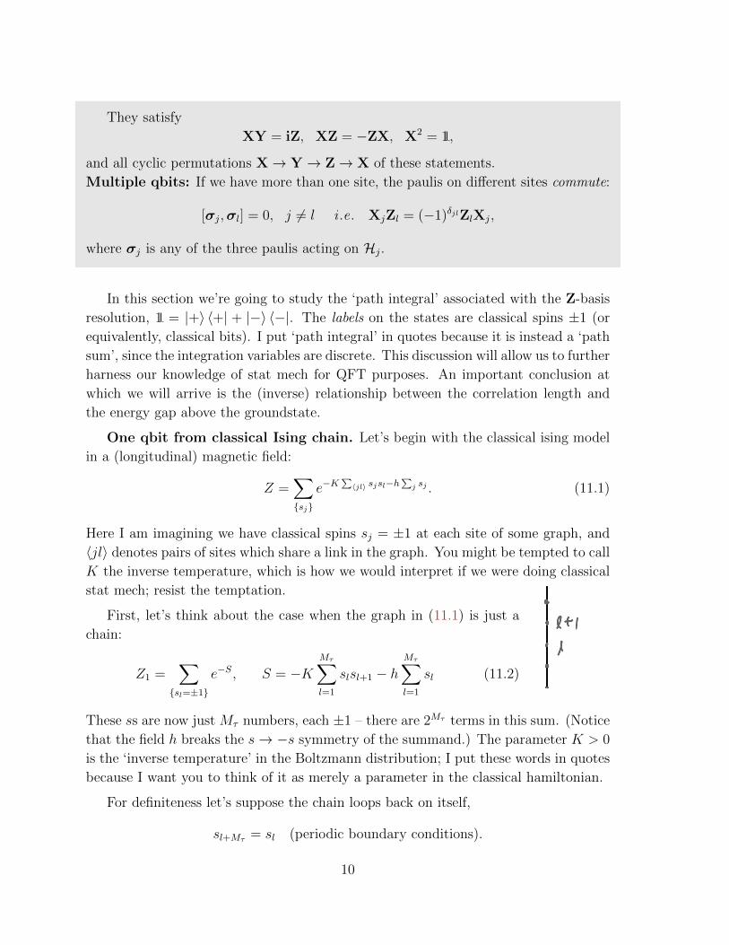
First, let’s think about the case when the graph in (11.1) is just a
chain:
Z1 =∑sl=±1
e−S, S = −KMτ∑l=1
slsl+1 − hMτ∑l=1
sl (11.2)
These ss are now just Mτ numbers, each ±1 – there are 2Mτ terms in this sum. (Notice
that the field h breaks the s→ −s symmetry of the summand.) The parameter K > 0
is the ‘inverse temperature’ in the Boltzmann distribution; I put these words in quotes
because I want you to think of it as merely a parameter in the classical hamiltonian.
For definiteness let’s suppose the chain loops back on itself,
sl+Mτ = sl (periodic boundary conditions).
10
Using the identity e∑l(...)l =
∏l e
(...)l ,
Z1 =∑sl
Mτ∏l=1
T1(sl, sl+1)T2(sl)
where
T1(s1, s2) ≡ eKs1s2 , T2(s) ≡ ehs .
What are these objects? The conceptual leap is to think of T1(s1, s2) as a 2×2 matrix:
T1(s1, s2) =
(eK e−K
e−K eK
)s1s2
= 〈s1|T1 |s2〉 ,
which we can then regard as matrix elements of an operator T1 acting on a 2-state
quantum system (hence the boldface). And we have to think of T2(s) as the diagonal
elements of the same kind of matrix:
δs1,s2T2(s1) =
(eh 0
0 e−h
)s1s2
= 〈s1|T2 |s2〉 .
So we have
Z1 = tr
(T1T2)(T1T2) · · · (T1T2)︸ ︷︷ ︸Mτ times
= trTMτ (11.3)
where I’ve written
T ≡ T122 T1T
122 = T† = Tt
for convenience (so it’s symmetric). This object is the transfer matrix. What’s the
trace over in (11.3)? It’s a single two-state system – a single qbit (or quantum spin)
that we’ve constructed from this chain of classical two-valued variables.
Even if we didn’t care about quantum spins, this way of organizing the partition
sum of the Ising chain does the sum for us (since the trace is basis-independent, and
so we might as well evaluate it in the basis where T is diagonal):
Z1 = trTMτ = λMτ+ + λMτ
−
where λ± are the two eigenvalues of the transfer matrix, λ+ ≥ λ−:
λ± = eK coshh±√e2K sinh2 h+ e−2K h→0→
2 coshK
2 sinhK.(11.4)
In the thermodynamic limit, Mτ 1, the bigger one dominates the free energy
e−F = Z1 = λMτ+
(1 +
(λ−λ+
)Mτ)∼ λMτ
+ .
11
Now I command you to think of the transfer matrix as
T = e−∆τH
the propagator in euclidean time (by an amount ∆τ), where H is the quantum hamil-
tonian operator for a single qbit (note the boldface to denote quantum operators). So
what’s H? To answer this, let’s rewrite the parts of the transfer matrix in terms of
paulis, thinking of s = ± as Z-eigenstates. For T2, which is diagonal in the Z basis,
this is easy:
T2 = ehZ.
To write T1 this way, stare at its matrix elements in the Z basis:
〈s1|T1 |s2〉 =
(eK e−K
e−K eK
)s1s2
and compare them to those of
eaX+b1 = ebeaX = eb (cosh a+ X sinh a)
which are
〈s1| eaX+b1 |s2〉 = eb(
cosh a sinh a
sinh a cosh a
)s1,s2
So we want eb sinh a = e−K , eb cosh a = eK which is solved by
e−2K = tanh a . (11.5)
So we want to identify
T1T2 = eb1+aXehZ ≡ e−∆τH
for small ∆τ . This requires that a, b, h scale like ∆τ , and so we can combine the
exponents. Assuming that ∆τ E−10 , h−1, the result is
H = E0 −∆
2X− hZ .
Here E0 = b∆τ, h = h
∆τ,∆ = 2a
∆τ. (Note that it’s not surprising that the Hamiltonian
for an isolated qbit is of the form H = d01 + ~d · ~σ, since these operators span the set
of hermitian operators on a qbit; but the relation between the parameters that we’ve
found will be important.)
To recap, let’s go backwards: consider the quantum system consisting of a single
spin with H = E0 − ∆2X + hZ . Set h = 0 for a moment. Then ∆ is the energy gap
12
between the groundstate and the first excited state (hence the name). The thermal
partition function is
ZQ(T ) = tre−H/T =∑s=±
〈s| e−βH |s〉 , (11.6)
where we’ve evaluated the trace in the Z basis, Z |s〉 = s |s〉. I emphasize that T here
is the temperature to which we are subjecting our quantum spin; β = 1T
is the length
of the euclidean time circle. Break up the euclidean time circle into Mτ intervals of size
∆τ = β/Mτ . Insert many resolutions of unity (this is called ‘Trotter decomposition’)
ZQ =∑
s1...sMτ
〈sMτ | e−∆τH |sMτ−1〉 〈sMτ−1| e−∆τH |sMτ−2〉 · · · 〈s1| e−∆τH |sMτ 〉 .
The RHS is the partition function of a classical Ising chain, Z1 in (11.2), with h = 0
and K given by (11.5), which in the present variables is:
e−2K = tanh
(β∆
2Mτ
). (11.7)
Notice that if our interest is in the quantum model with couplings E0,∆, we can use
any Mτ we want – there are many classical models we could use1. For given Mτ , the
couplings we should choose are related by (11.7).
A quantum system with just a single spin (for any H not proportional to 1) clearly
has a unique groundstate; this statement means the absence of a phase transition in
the 1d Ising chain.
More than one spin.2 Let’s do that procedure again, this time supposing the
graph in question is a cubic lattice with more than one dimension, and let’s think of
one of the directions as euclidean time, τ . We’ll end up with more than one spin.
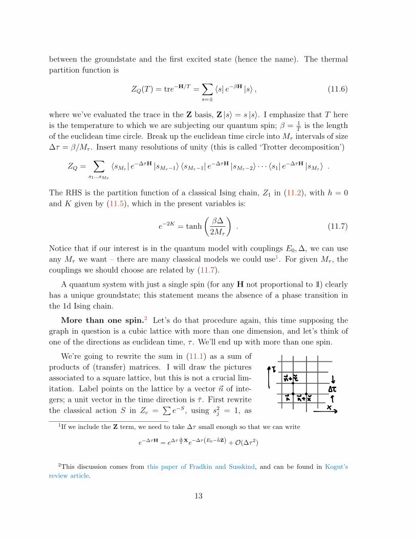
We’re going to rewrite the sum in (11.1) as a sum of
products of (transfer) matrices. I will draw the pictures
associated to a square lattice, but this is not a crucial lim-
itation. Label points on the lattice by a vector ~n of inte-
gers; a unit vector in the time direction is τ . First rewrite
the classical action S in Zc =∑e−S, using s2
j = 1, as
1If we include the Z term, we need to take ∆τ small enough so that we can write
e−∆τH = e∆τ ∆2 Xe−∆τ(E0−hZ) +O(∆τ2)
2This discussion comes from this paper of Fradkin and Susskind, and can be found in Kogut’s
review article.
13
S = −∑~n
(Ks(~n+ τ)s(~n) +Kxs(~n+ x)s(~n))
= K∑~n
(1
2(s(~n+ τ)− s(~n))2 − 1
)−Kx
∑~n
s(~n+ x)s(~n)
= const +∑
rows at fixed time, l
L(l + 1, l) (11.8)
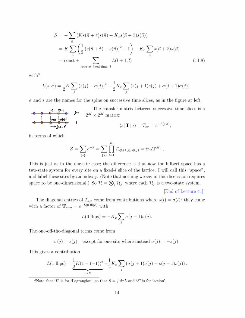
with3
L(s, σ) =1
2K∑j
(s(j)− σ(j))2 − 1
2Kx
∑j
(s(j + 1)s(j) + σ(j + 1)σ(j)) .
σ and s are the names for the spins on successive time slices, as in the figure at left.
The transfer matrix between successive time slices is a
2M × 2M matrix:
〈s|T |σ〉 = Tsσ = e−L(s,σ),
in terms of which
Z =∑s
e−S =∑s
Mτ∏l=1
Ts(l+1,j),s(l,j) = trHTMτ .
This is just as in the one-site case; the difference is that now the hilbert space has a
two-state system for every site on a fixed-l slice of the lattice. I will call this “space”,
and label these sites by an index j. (Note that nothing we say in this discussion requires
space to be one-dimensional.) So H =⊗
jHj, where each Hj is a two-state system.
[End of Lecture 41]
The diagonal entries of Ts,σ come from contributions where s(l) = σ(l): they come
with a factor of Ts=σ = e−L(0 flips) with
L(0 flips) = −Kx
∑j
σ(j + 1)σ(j).
The one-off-the-diagonal terms come from
σ(j) = s(j), except for one site where instead σ(j) = −s(j).
This gives a contribution
L(1 flips) =1
2K(1− (−1))2︸ ︷︷ ︸
=2K
−1
2Kx
∑j
(σ(j + 1)σ(j) + s(j + 1)s(j)) .
3Note that ‘L’ is for ‘Lagrangian’, so that S =∫dτL and ‘S’ is for ‘action’.
14
Similarly,
L(n flips) = 2nK − 1
2Kx
∑j
(σ(j + 1)σ(j) + s(j + 1)s(j)) .
Now we need to figure out who is H, as defined by
T = e−∆τH ' 1−∆τH ;
we want to consider ∆τ small and must choose Kx, K to make it so. We have to match
the matrix elements 〈s|T |σ〉 = Tsσ:
T (0 flips)sσ = δsσeKx∑j s(j)s(j+1) ' 1 −∆τH|0 flips
T (1 flip)sσ = e−2Ke12Kx∑j(σ(j+1)σ(j)+s(j+1)s(j)) ' −∆τH|1 flip
T (n flips)sσ = e−2nKe12Kx∑j(σ(j+1)σ(j)+s(j+1)s(j)) ' −∆τH|n flips (11.9)
From the first line, we learn that Kx ∼ ∆τ ; from the second we learn e−2K ∼ ∆τ ; we’ll
call the ratio which we’ll keep finite g ≡ K−1x e−2K . To make τ continuous, we take
K →∞, Kx → 0, holding g fixed. Then we see that the n-flip matrix elements go like
e−nK ∼ (∆τ)n and can be ignored – the hamlitonian only has 0- and 1-flip terms.
To reproduce (11.9), we must take
HTFIM = −J
(g∑j
Xj +∑j
Zj+1Zj
).
Here J is a constant with dimensions of energy that we pull out of ∆τ . The first term
is the ‘one-flip’ term; the second is the ‘zero-flips’ term. The first term is a ‘transverse
magnetic field’ in the sense that it is transverse to the axis along which the neighboring
spins interact. So this is called the transverse field ising model. In D = 1 + 1 it can be
understood completely, and I hope to say more about it later this quarter. As we’ll see,
it contains the universal physics of the 2d Ising model, including Onsager’s solution.
The word ‘universal’ requires some discussion.
Symmetry of the transverse field quantum Ising model: HTFIM has a Z2
symmetry, generated by S =∏
j Xj, which acts by
SZj = −ZjS, SXj = +XjS, ∀j;
On Z eigenstates it acts as:
S |sjj〉 = |−sjj〉 .
15
It is a symmetry in the sense that:
[HTFIM,S] = 0.
Notice that S2 =∏
j X2j = 1,, and S = S† = S−1.
By ‘a Z2 symmetry,’ I mean that the symmetry group consists of two elements
G = 1,S, and they satisfy S2 = 1, just like the group 1,−1 under multiplication.
This group is G = Z2. (For a bit of context, the group ZN is realized by the Nth roots
of unity, under multiplication.)
The existence of this symmetry of the quantum model is a direct consequence of the
fact that the hamiltonian of the classical system (the action S[s]) was invariant under
the operation sj → −sj,∀j. This meant that the matrix elements of the transfer matrix
satisfy Ts,s′ = T−s,−s′ which implies the symmetry of H. (Note that symmetries of the
classical action do not so immediately imply symmetries of the associated quantum
system if the system is not as well-regulated as ours is. This is the phenomenon called
‘anomaly’.)
Quantum Ising in d space dimensions to classical Ising in d+ 1 dims
[Sachdev, 2d ed p. 75] Just to make sure it’s nailed down, let’s go backwards again.
The partition function of the quantum Ising model at temperature T is
ZQ(T ) = tr⊗Mj=1Hj
e−1T
HI = tr(e−∆τHI
)Mτ
The transfer matrix here e−∆τHI is a 2M × 2M matrix. We’re going to take ∆τ →0,Mτ →∞, holding 1
T= ∆Mτ fixed. Let’s use the usual4 ‘split-step’ trick of breaking
up the non-commuting parts of H:
e−∆τHI ≡ TxTz +O(∆τ 2).
Tx ≡ eJg∆τ∑j Xj , Tz ≡ eJ∆τ
∑j ZjZj+1 .
Now insert a resolution of the identity in the Z-basis,
1 =∑sjMj=1
|sj〉 〈sj| , Zj |sj〉 = sj |sj〉 , sj = ±1.
4By ‘usual’ I mean that this is just like in the path integral of a 1d particle, when we write
e−∆τH = e−∆τ2mp2
e−∆τV (q) +O(∆τ2).
16
many many times, one between each pair of transfer operators; this turns the transfer
operators into transfer matrices. The Tz bit is diagonal, by design:
Tz |sj〉 = eJ∆τ∑j sjsj+1 |sj〉 .
The Tx bit is off-diagonal, but only on a single spin at a time:⟨s′j
∣∣Tx |sj〉 =∏j
⟨s′j∣∣ eJg∆τXj |sj〉︸ ︷︷ ︸
2×2
Acting on a single spin at site j, this 2 × 2 matrix is just the one from the previous
discussion:⟨s′j∣∣ eJg∆τXj |sj〉 = e−beKs
′jsj , e−b =
1
2cosh (2Jg∆τ) , e−2K = tanh (Jg∆τ) .
Notice that it wasn’t important to restrict to 1 + 1 dimensions here. The only differ-
ence is in the Tz bit, which gets replaced by a product over all neighbors in higher
dimensions: ⟨s′j
∣∣Tz |sj〉 = δs,s′eJ∆τ
∑〈jl〉 sjsl
where 〈jl〉 denotes nearest neighbors, and the innocent-looking δs,s′ sets the spins
sj = s′j equal for all sites.
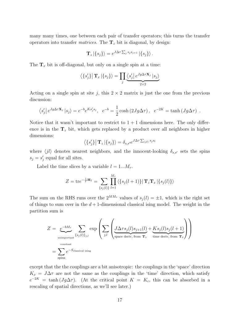
Label the time slices by a variable l = 1...Mτ .
Z = tre−1T
HI =∑sj(l)
Mτ∏l=1
〈sj(l + 1)|TzTx |sj(l)〉
The sum on the RHS runs over the 2MMτ values of sj(l) = ±1, which is the right set
of things to sum over in the d+ 1-dimensional classical ising model. The weight in the
partition sum is
Z = e−bMτ︸ ︷︷ ︸unimportant
constant
∑sj(l)j,l
exp
∑j,l
J∆τsj(l)sj+1(l)︸ ︷︷ ︸space deriv, from Tz
+Ksj(l)sj(l + 1)︸ ︷︷ ︸time deriv, from Tx
=∑spins
e−Sclassical ising
except that the the couplings are a bit anisotropic: the couplings in the ‘space’ direction
Kx = J∆τ are not the same as the couplings in the ‘time’ direction, which satisfy
e−2K = tanh (Jg∆τ). (At the critical point K = Kc, this can be absorbed in a
rescaling of spatial directions, as we’ll see later.)
17
Dictionary. So this establishes a mapping between classical systems in d + 1 di-
mensions and quantum systems in d space dimensions. Here’s the dictionary:
statistical mechanics in d+ 1 dimensions quantum system in d space dimensions
transfer matrix euclidean-time propagator, e−∆τH
statistical ‘temperature’ (lattice-scale) coupling K
free energy in infinite volume groundstate energy: e−F = Z = tre−βH β→0→ e−βE0
periodicity of euclidean time Lτ temperature: β = 1T
= ∆τMτ
statistical averagesgroundstate expectation values
of time-ordered operators
Note that this correspondence between classical and quantum systems is not an iso-
morphism. For one thing, we’ve seen that many classical systems are related to the
same quantum system, which does not care about the lattice spacing in time. There is
a set of physical quantities which agree between these different classical systems, called
universal, which is the information in the quantum system. More on this below.
Consequences for phase transitions and quantum phase transitions.
One immediate consequence is the following. Think about what happens at a
phase transition of the classical problem. This means that the free energy F (K, ...)
has some kind of singularity at some value of the parameters, let’s suppose it’s the
statistical temperature, i.e. the parameter we’ve been calling K. ‘Singularity’ means
breakdown of the Taylor expansion, i.e. a disagreement between the actual behavior
of the function and its Taylor series – a non-analyticity. First, this can only happen in
the thermodynamic limit (at the very least Mτ → ∞), since otherwise there are only
a finite number of terms in the partition sum and F is an analytic function of K (it’s
a polynomial in e−K).
An important dichotomy is between continuous phase transitions (also called second
order or higher) and first-order phase transitions; at the latter, ∂KF is discontinous at
the transition, at the former it is not. This seems at first like an innocuous distinction,
but think about it from the point of view of the transfer matrix for a moment. In the
thermodynamic limit, Z = λ1(K)Mτ , where λ1(K) is the largest eigenvalue of T(K).
How can this have a singularity in K? There are two possibilities:
18
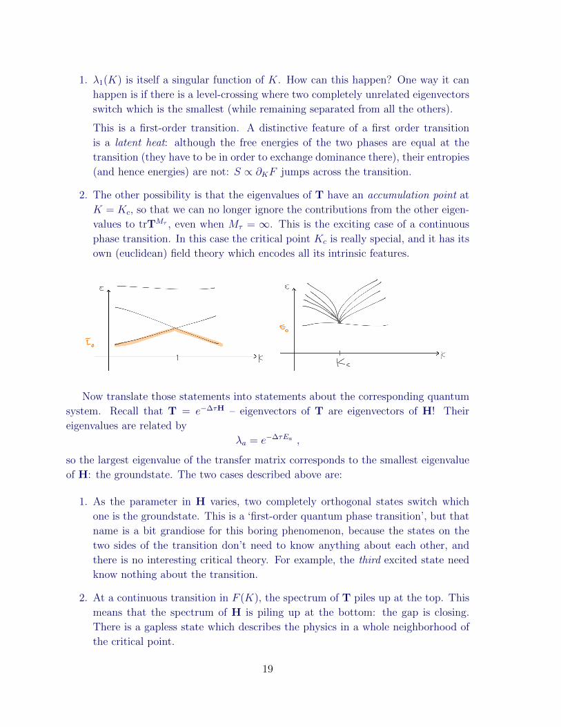
1. λ1(K) is itself a singular function of K. How can this happen? One way it can
happen is if there is a level-crossing where two completely unrelated eigenvectors
switch which is the smallest (while remaining separated from all the others).
This is a first-order transition. A distinctive feature of a first order transition
is a latent heat: although the free energies of the two phases are equal at the
transition (they have to be in order to exchange dominance there), their entropies
(and hence energies) are not: S ∝ ∂KF jumps across the transition.
2. The other possibility is that the eigenvalues of T have an accumulation point at
K = Kc, so that we can no longer ignore the contributions from the other eigen-
values to trTMτ , even when Mτ = ∞. This is the exciting case of a continuous
phase transition. In this case the critical point Kc is really special, and it has its
own (euclidean) field theory which encodes all its intrinsic features.
Now translate those statements into statements about the corresponding quantum
system. Recall that T = e−∆τH – eigenvectors of T are eigenvectors of H! Their
eigenvalues are related by
λa = e−∆τEa ,
so the largest eigenvalue of the transfer matrix corresponds to the smallest eigenvalue
of H: the groundstate. The two cases described above are:
1. As the parameter in H varies, two completely orthogonal states switch which
one is the groundstate. This is a ‘first-order quantum phase transition’, but that
name is a bit grandiose for this boring phenomenon, because the states on the
two sides of the transition don’t need to know anything about each other, and
there is no interesting critical theory. For example, the third excited state need
know nothing about the transition.
2. At a continuous transition in F (K), the spectrum of T piles up at the top. This
means that the spectrum of H is piling up at the bottom: the gap is closing.
There is a gapless state which describes the physics in a whole neighborhood of
the critical point.
19
Using the quantum-to-classical dictionary, the groundstate energy of the TFIM at
the transition reproduces Onsager’s tour-de-force free energy calculation.
Another failure mode of this correspondence: there are some quantum systems
which when Trotterized produce a stat mech model with non-positive Boltzmann
weights, i.e. e−S < 0 for some configurations; this requires the classical hamilto-
nian S to be complex. These models are less familiar! An example where this happens
is the spin-12
Heisenberg (≡ SU(2)-invariant) chain, as you’ll see on the homework. This
is a manifestation of a sign problem, which is a general term for a situation requiring
adding up a bunch of numbers which aren’t all positive, and hence may involve large
cancellations. Sometimes such a problem can be removed by cleverness, sometimes it
is a fundamental issue of computational complexity.
The quantum phase transitions of such quantum systems are not just ordinary finite-
temperature transitions of familiar classical stat mech systems. So for the collector of
QFTs, there is something to be gained by studying quantum phase transitions.
Correlation functions. [Sachdev, 2d ed p. 69] For now, let’s construct correlation
functions of spins in the classical Ising chain, (11.2), using the transfer matrix. (We’ll
study correlation functions in the TFIM later, I think.) Let
C(l, l′) ≡ 〈slsl′〉 =1
Z1
∑sll
e−Hcslsl′
By translation invariance, this is only a function of the difference C(l, l′) = C(l − l′).For simplicity, set the external field h = 0. Also, assume that l′ > l (as we’ll see, this
is time-ordering of the correlation function). In terms of the transfer matrix, it is:
C(l − l′) =1
Ztr(TMτ−l′ZTl′−lZTl
). (11.10)
Notice that there is only one operator Z = σz here; it is the matrix
Zss′ = δss′s .
All the information about the index l, l′ is encoded in the location in the trace.
Let’s evaluate this trace in the basis of T eigenstates. When h = 0, we have
T = eK1 + e−KX, so these are X eigenstates:
T |→〉 = λ+ |→〉 , T |←〉 = λ− |→〉 .
Here |→〉 ≡ 1√2
(|↑〉+ |↓〉).
20
In this basis
〈α|Z |β〉 =
(0 1
1 0
)αβ
, α, β =→ or ← .
So the trace (aka path integral) has two terms: one where the system spends l′ − l
steps in the state |→〉 (and the rest in |←〉), and one where it spends l′− l steps in the
state |→〉. The result (if we take Mτ →∞ holding fixed l′ − l) is
C(l′ − l) =λMτ−l′+l
+ λl′−l− + λMτ−l′+l
− λl′−l
+
λMτ+ + λMτ
−
Mτ→∞→ tanhl′−lK . (11.11)
You should think of the insertions as
sl = Z(τ), τ = ∆τ l.
So what we’ve just computed is
C(τ) = 〈Z(τ)Z(0)〉 = tanhlK = e−|τ |/ξ (11.12)
where the correlation time ξ satisfies
1
ξ=
1
∆τln cothK . (11.13)
Notice that this is the same as our formula for the gap, ∆, in (11.7).5 This connection
between the correlation length in euclidean time and the energy gap is general and
important.
For large K, ξ is much bigger than the lattice spacing:
ξ
∆τ
K1' 1
2e2K 1.
This is the limit we had to take to make the euclidean time continuous.
5Seeing this requires the following cool hyperbolic trig fact:
If e−2K = tanhX then e−2X = tanhK (11.14)
(i.e. this equation is ‘self-dual’) which follows from algebra. Here (11.7) says X = ∆TMτ
= ∆τ∆ while
(11.13) says X = ∆τ/ξ. Actually this relation (11.14) can be made manifestly symmetric by writing
it as
1 = sinh 2X sinh 2K .
(You may notice that this is the same combination that appears in the Kramers-Wannier self-duality
condition.) I don’t know a slick way to show this, but if you just solve this quadratic equation for
e−2K and boil it enough, you’ll find tanhX.
21
Notice that if we had taken l < l′ instead, we would have found the same answer
with l′ − l replaced by l − l′.
[End of Lecture 42]
Continuum scaling limit and universality
[Sachdev, 2d ed §5.5.1, 5.5.2] Now we are going to grapple with the term ‘universal’.
Let’s think about the Ising chain some more. We’ll regard Mτ∆τ as a physical quantity,
the proper length of the chain. We’d like to take a continuum limit, where Mτ →∞ or
∆τ → 0 or maybe both. Such a limit is useful if ξ ∆τ . This decides how we should
scale K,h in the limit. More explicitly, here is the prescription: Hold fixed physical
quantities (i.e. eliminate the quantities on the RHS of these expressions in favor of
those on the LHS):
the correlation length, ξ ' ∆τ1
2e2K ,
the length of the chain, Lτ = ∆τMτ ,
physical separations between operators, τ = (l − l′)∆τ,the applied field in the quantum system, h = h/∆τ. (11.15)
while taking ∆τ → 0, K →∞,Mτ →∞.
What physics of the various chains will agree? Certainly only quantities that don’t
depend explicitly on the lattice spacing; such quantities are called universal.
Consider the thermal free energy of the single quantum spin (11.6)6: The energy
spectrum of our spin is E± = E0 ±√
(∆/2)2 + h2, which means
F = −T logZQ = E0 − T ln
(2 cosh
(β√
(∆/2)2 + h2
))(just evaluate the trace in the energy eigenbasis). In fact, this is just the behavior of
the ising chain partition function in the scaling limit (11.15), since, in the limit (11.4)
becomes
λ± '√
2ξ
∆τ
(1± ∆τ
2ξ
√1 + 4h2ξ2
)and so in the scaling limit (11.15)
F ' Lτ
− K
∆τ︸ ︷︷ ︸cutoff-dependent vac. energy
− 1
Lτln
(2 cosh
Lτ2
√ξ−2 + 4h2
) ,
which is the same (up to an additive constant) as the quantum formula under the
previously-made identifications T = 1Lτ, ξ−1 = ∆.
6[Sachdev, 1st ed p. 19, 2d ed p. 73]
22
We can also use the quantum system to compute the correlation functions of the
classical chain in the scaling limit (11.11). They are time-ordered correlation functions:
C(τ1 − τ2) = Z−1Q tre−βH (θ(τ1 − τ2)Z(τ1)Z(τ2) + θ(τ2 − τ1)Z(τ2)Z(τ1))
where
Z(τ) ≡ eHτZe−Hτ .
This time-ordering is just the fact that we had to decide whether l′ or l was bigger in
(11.10).
For example, consider what happens to this when T → 0. Then (inserting 1 =∑n |n〉 〈n|, in an energy eigenbasis H |n〉 = En |n〉),
C(τ)|T=0 =∑n
| 〈0|Z |n〉 |2e−(En−E0)|τ |
where the |τ | is taking care of the time-ordering. This is a spectral representation of the
correlator. For large τ , the contribution of |n〉 is exponentially suppressed by its energy,
so the sum is approximated well by the lowest energy state for which the matrix element
is nonzero. Assuming this is the first excited state (which in our two-state system it
has no choice!), we have
C(τ)|T=0τ→∞' e−τ/ξ, ξ = 1/∆,
where ∆ is the energy gap.
In these senses, the quantum theory of a single qbit is the universal theory of the
Ising chain. For example, if we began with a chain that had in addition next-nearest-
neighbor interactions, ∆Hc = K ′∑
j s(j)s(j + 2), we could redo the procedure above.
The scaling limit would not be exactly the same; we would have to scale K ′ somehow
(it would also have to grow in the limit). But we would find the same 2-state quantum
system, and when expressed in terms of physical variables, the ∆τ -independent terms
in F would be identical, as would the form of the correlation functions, which is
C(τ) = 〈Z(τ)Z(0)〉 =e−|τ |/ξ + e−(Lτ−|τ |)/ξ
1 + e−Lτ/ξ.
(Note that in this expression we did not assume |τ | Lτ as we did before in (11.12),
to which this reduces in that limit.)
23
11.2 Interlude on differential forms and algebraic topology
The next item of business is coherent state path integrals of all kinds. We are going to
make a sneak attack on them.
[Zee section IV.4] We interrupt this physics discussion with a message from our
mathematical underpinnings. This is nothing fancy, mostly just some book-keeping.
It’s some notation that we’ll find useful. As a small payoff we can define some simple
topological invariants of smooth manifolds.
Suppose we are given a smooth manifold X on which we can do calculus. For now,
we don’t even need a metric on X.
A p-form on X is a completely antisymmetric p-index tensor,
A ≡ 1
p!Am1...mpdx
m1 ∧ ... ∧ dxmp .
The coordinate one-forms are fermionic objects in the sense that dxm1∧dxm2 = −dxm2∧dxm1 and (dx)2 = 0. The point in life of a p-form is that it can be integrated over
a p-dimensional space. The order of its indices keeps track of the orientation (and it
saves us the trouble of writing them). It is a geometric object, in the sense that it is
something that can be (wants to be) integrated over a p-dimensional subspace of X,
and its integral will only depend on the subspace, not on the coordinates we use to
describe it.
Familiar examples include the gauge potential A = Aµdxµ, and its field strength
F = 12Fµνdx
µ ∧ dxν . Given a curve C in X parameterized as xµ(s), we have∫C
A ≡∫C
dxµAµ(x) =
∫dsdxµ
dsAµ(x(s))
and this would be the same if we chose some other parameterization or some other
local coordinates.
The wedge product of a p-form A and a q-form B is a p+ q form
A ∧B = Am1..mpBmp+1...mp+qdxm1 ∧ ... ∧ dxmq ,
7 The space of p-forms on a manifold X is sometimes denoted Ωp(X), especially when
7The components of A ∧B are then
(A ∧B)m1...mp+q =(p+ q)!
p!q!A[m1...mpBmp+1...mp+q ]
where [..] means sum over permutations with a −1 for odd permutations. Try not to get caught up
in the numerical prefactors.
24
it is to be regarded as a vector space (let’s say over R).
The exterior derivative d acts on forms as
d : Ωp(X) → Ωp+1(X)
A 7→ dA
by
dA = ∂m1 (A)m2...mp+1dxm1 ∧ ... ∧ dxmp+1
1
(p+ 1)!.
You can check that
d2 = 0
basically because derivatives commute. Notice that F = dA in the example above.
Denoting the boundary of a region D by ∂D, Stokes’ theorem is∫D
dα =
∫∂D
α.
And notice that Ωp>dim(X)(X) = 0 – there are no forms of rank larger than the
dimension of the space.
A form ωp is closed if it is killed by d: dωp = 0.
A form ωp is exact if it is d of something: ωp = dαp−1. That something must be a
(p− 1)-form.
Because of the property d2 = 0, it is possible to define cohomology – the image of
one d : Ωp → Ωp+1 is in the kernel of the next d : Ωp+1 → Ωp+2 (i.e. the Ωps form a
chain complex). The pth de Rham cohomology group of the space X is defined to be
Hp(X) ≡ closed p-forms on X
exact p-forms on X=
ker (d) ∈ Ωp
Im (d) ∈ Ωp.
That is, two closed p-forms are equivalent in cohomology if they differ by an exact
form:
[ωp]− [ωp + dαp−1] = 0 ∈ Hp(X),
where [ωp] denotes the equivalence class. The dimension of this group is bp ≡ dimHp(X)
called the pth betti number and is a topological invariant of X. The euler characteristic
of X, which you can get by triangulating X and counting edges and faces and stuff is
χ(X) =
d=dim(X)∑p=0
(−1)pbp(X).
25

Here’s a very simple example, where X = S1 is a circle. x ' x+ 2π is a coordinate;
the radius will not matter since it can be varied continuously. An element of Ω0(S1) is
a smooth periodic function of x. An element of Ω1(S1) is of the form A1(x)dx where
A1 is a smooth periodic function. Every such element is closed because there are no
2-forms on a 1d space. The exterior derivative on a 0-form is
dA0(x) = A′0dx
Which 0-forms are closed? A′0 = 0 means A0 is a constant. Which 1-forms can we
make this way? The only one we can’t make is dx itself, because x is not a periodic
function. Therefore b0(S1) = b1(S1) = 1.
Now suppose we have a volume element on X, i.e. a way of integrating d-forms.
This is guaranteed if we have a metric, since then we can integrate∫ √
det g..., but is
less structure. Given a volume form, we can define the Hodge star operation ? which
maps a p-form into a (d− p)-form:
? : Ωp → Ωd−p
by (?A(p)
)µ1...µd−p
≡ εµ1...µdA(p) µd−p+1...µd
An application: consider the Maxwell action, 14FµνF
µν . You can show that this is
the same as S[A] =∫F ∧ ?F . (Don’t trust my numerical prefactor.) You can derive
the Maxwell EOM by 0 = δSδA
.∫F ∧F is the θ term. The magnetic dual field strength
is F = ?F . Many generalizations of duality can be written naturally using the Hodge
? operation.
As you can see from the Maxwell example, the Hodge star gives an inner product
on Ωp: for two p-forms α, β (α, β) =∫α ∧ ?β), (α, α) ≥ 0. We can define the adjoint
of d with respect to the inner product by∫d†α ∧ ?β = (d†α, β) ≡ (α, dβ) =
∫α ∧ ?dβ
Combining this relation with integration by parts, we find d† = ± ? d?.
We can make a Laplacian on forms by
∆ = dd† + d†d.
This is a supersymmetry algebra, in the sense that d, d† are grassmann operators.
26
Any cohomology class [ω] has a harmonic representative, [ω] = [ω] where in addition
to being closed dω = dω = 0, it is co-closed, 0 = d†ω, and hence harmonic ∆ω = 0.
I mention this because it implies Poincare duality: bp(X) = bd−p(X) if X has a
volume form. This follows because the mapHp → Hd−p [ωp] 7→ [?ωp] is an isomorphism.
(Choose the harmonic representative, it has d ? ωp = 0.)
The de Rham complex of X can be realized as the groundstates of a physical system,
namely the supersymmetric nonlinear sigma model with target space X. The fermions
play the role of the dxµs. The states are of the form
|A〉 =d∑p=1
Aµ1···µp(x)ψµ1ψµ2 · · ·ψµp |0〉
where ψ are some fermion creation operators. This shows that the hilbert space is the
space of forms on X, that is H ' Ω(X) = ⊕pΩp(X). The supercharges act like d and
d† and therefore the supersymmetric groundstates are (harmonic representatives of)
cohomology classes.
This machinery will be very useful to us. I use it all the time.
[End of Lecture 43]
11.3 Coherent state path integrals for spin systems
11.3.1 Geometric quantization and coherent state quantization of spin sys-
tems
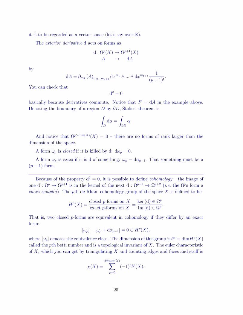
[Zinn-Justin, Appendix A3; XGW §2.3] We’re go-
ing to spend some time talking about QFT in
D = 0+1, then we’ll work our way up to D = 1+1,
and beyond. Consider the nice, round two-sphere.
It has an area element which can be written
ω = sd cos θ ∧ dϕ and satisfies
∫S2
ω = 4πs.
s is a number. Suppose we think of this sphere as the phase space of some dynamical
system. We can use ω as the symplectic form. What is the associated quantum
mechanics system?
27
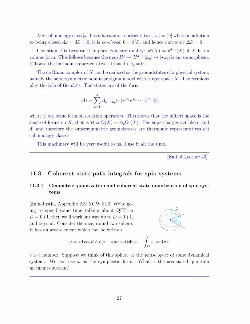
Let me remind you what I mean by ‘the sym-
plectic form’. Recall the phase space formulation
of classical dynamics. The action associated to a
trajectory is
A[x(t), p(t)] =
∫ t2
t1
dt (px−H(x, p)) =
∫γ
p(x)dx−∫Hdt
where γ is the trajectory through the phase space. The first term is the area ‘under
the graph’ in the classical phase space – the area between (p, x) and (p = 0, x). We
can rewrite it as ∫p(t)x(t)dt =
∫∂D
pdx =
∫D
dp ∧ dx
using Stokes’ theorem; here ∂D is the closed curve made by the classical trajectory and
some reference trajectory (p = 0) and it bounds some region D. Here ω = dp ∧ dx is
the symplectic form. More generally, we can consider an 2n-dimensional phase space
with coordinates uα, α = 1..2n and symplectic form
ω = ωαβduα ∧ duβ
and action
A[u] =
∫D
ω −∫∂D
dtH(u, t).
The symplectic form says who is canonically conjugate to whom. It’s important that
dω = 0 so that the equations of motion resulting from A depend only on the trajectory
γ = ∂D and not on the interior of D. The equations of motion from varying u are
ωαβuβ =
∂H
∂uα.
Locally, we can find coordinates p, x so that ω = d(pdx). Globally on the phase
space this is not guaranteed – the symplectic form needs to be closed, but need not be
exact.
So the example above of the two-sphere is one where the symplectic form is closed
(there are no three-forms on the two sphere, so dω = 0 automatically), but is not exact.
One way to see that it isn’t exact is that if we integrate it over the whole two-sphere,
we get the area: ∫S2
ω = 4πs .
On the other hand, the integral of an exact form over a closed manifold (meaning a
manifold without boundary, like our sphere) is zero:∫C
dα =
∫∂C
α = 0.
28
So there can’t be a globally defined one-form α such that dα = ω. Locally, we can find
one; for example:
α = s cos θdϕ ,
but this is singular at the poles, where ϕ is not a good coordinate.
So: what I mean by “what is the associated quantum system...” is the following:
let’s construct a system whose path integral is
Z =
∫[dθdϕ]e
i~A[θ,ϕ] (11.16)
with the action above, and where [dx] denotes the path integral measure:
[dx] ≡ ℵN∏i=1
dx(ti)
where ℵ involves lots of awful constants that drop out of ratios. It is important that
the measure does not depend on our choice of coordinates on the sphere.
• Hint 1: the model has an action of O(3), by rotations of the sphere.
• Hint 2: We actually didn’t specify the model yet, since we didn’t choose the
Hamiltonian. For definiteness, let’s pick the hamiltonian to be
H = −s~h · ~n
where ~n ≡ (sin θ cosϕ, sin θ sinϕ, cos θ). WLOG, we can take the polar axis to
be along the ‘magnetic field’: ~h = zh. The equations of motion are then
0 =δAδθ(t)
= −s sin θ (ϕ− h) , 0 =δAδϕ(t)
= −∂t (s cos θ)
which by rotation invariance can be written better as
∂t~n = ~h× ~n. (11.17)
This is a big hint about the answer to the question.
• Hint 3: Semiclassical expectations. Semiclassically, each patch of phase space
of area ~ contributes one quantum state. Therefore we expect that if our whole
phase space has area 4πs, we should get approximately 4πs2π~ = 2s
~ states, at least
at large s/~. (Notice that s appears out front of the action.) This will turn out
to be very close – the right answer is 2s+ 1 (when the spin is measured in units
with ~ = 1)!
29
[from Witten]
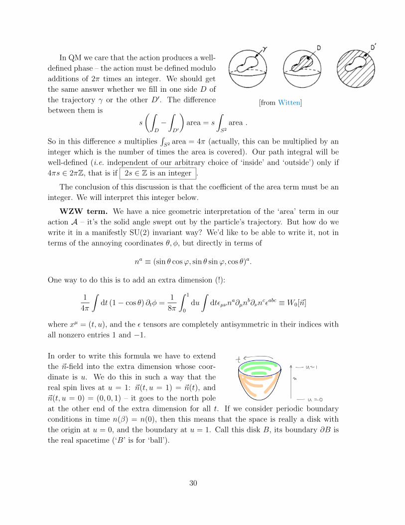
In QM we care that the action produces a well-
defined phase – the action must be defined modulo
additions of 2π times an integer. We should get
the same answer whether we fill in one side D of
the trajectory γ or the other D′. The difference
between them is
s
(∫D
−∫D′
)area = s
∫S2
area .
So in this difference s multiplies∫S2 area = 4π (actually, this can be multiplied by an
integer which is the number of times the area is covered). Our path integral will be
well-defined (i.e. independent of our arbitrary choice of ‘inside’ and ‘outside’) only if
4πs ∈ 2πZ, that is if 2s ∈ Z is an integer .
The conclusion of this discussion is that the coefficient of the area term must be an
integer. We will interpret this integer below.
WZW term. We have a nice geometric interpretation of the ‘area’ term in our
action A – it’s the solid angle swept out by the particle’s trajectory. But how do we
write it in a manifestly SU(2) invariant way? We’d like to be able to write it, not in
terms of the annoying coordinates θ, φ, but directly in terms of
na ≡ (sin θ cosϕ, sin θ sinϕ, cos θ)a.
One way to do this is to add an extra dimension (!):
1
4π
∫dt (1− cos θ) ∂tφ =
1
8π
∫ 1
0
du
∫dtεµνn
a∂µnb∂νn
cεabc ≡ W0[~n]
where xµ = (t, u), and the ε tensors are completely antisymmetric in their indices with
all nonzero entries 1 and −1.
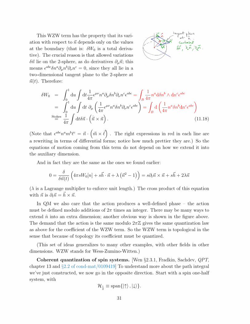
In order to write this formula we have to extend
the ~n-field into the extra dimension whose coor-
dinate is u. We do this in such a way that the
real spin lives at u = 1: ~n(t, u = 1) = ~n(t), and
~n(t, u = 0) = (0, 0, 1) – it goes to the north pole
at the other end of the extra dimension for all t. If we consider periodic boundary
conditions in time n(β) = n(0), then this means that the space is really a disk with
the origin at u = 0, and the boundary at u = 1. Call this disk B, its boundary ∂B is
the real spacetime (‘B’ is for ‘ball’).
30
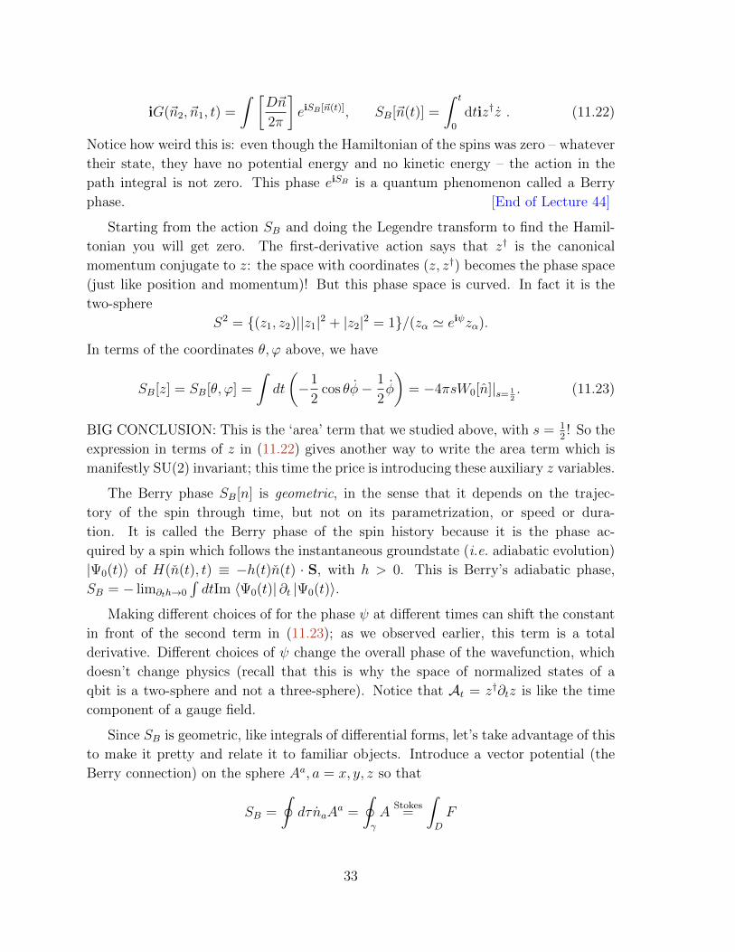
This WZW term has the property that its vari-
ation with respect to ~n depends only on the values
at the boundary (that is: δW0 is a total deriva-
tive). The crucial reason is that allowed variations
δ~n lie on the 2-sphere, as do derivatives ∂µ~n; this
means εabcδna∂µnb∂νn
c = 0, since they all lie in a
two-dimensional tangent plane to the 2-sphere at
~n(t). Therefore:
δW0 =
∫ 1
0
du
∫dt
1
4πεµνna∂µδn
b∂νncεabc =
∫B
1
4πnadδnb ∧ dncεabc
=
∫ 1
0
du
∫dt ∂µ
(1
4πεµνnaδnb∂νn
cεabc)
=
∫B
d
(1
4πnaδnbdncεabc
)Stokes
=1
4π
∫dtδ~n ·
(~n× ~n
). (11.18)
(Note that εabcnamb`c = ~n ·(~m× ~
). The right expressions in red in each line are
a rewriting in terms of differential forms; notice how much prettier they are.) So the
equations of motion coming from this term do not depend on how we extend it into
the auxiliary dimension.
And in fact they are the same as the ones we found earlier:
0 =δ
δ~n(t)
(4πsW0[n] + s~h · ~n+ λ
(~n2 − 1
))= s∂t~n× ~n+ s~h+ 2λ~n
(λ is a Lagrange multiplier to enforce unit length.) The cross product of this equation
with ~n is ∂t~n = ~h× ~n.
In QM we also care that the action produces a well-defined phase – the action
must be defined modulo additions of 2π times an integer. There may be many ways to
extend n into an extra dimension; another obvious way is shown in the figure above.
The demand that the action is the same modulo 2πZ gives the same quantization law
as above for the coefficient of the WZW term. So the WZW term is topological in the
sense that because of topology its coefficient must be quantized.
(This set of ideas generalizes to many other examples, with other fields in other
dimensions. WZW stands for Wess-Zumino-Witten.)
Coherent quantization of spin systems. [Wen §2.3.1, Fradkin, Sachdev, QPT,
chapter 13 and §2.2 of cond-mat/0109419] To understand more about the path integral
we’ve just constructed, we now go in the opposite direction. Start with a spin one-half
system, with
H 12≡ span|↑〉 , |↓〉.
31

Define spin coherent states |~n〉 by8:
~σ · ~n |~n〉 = |~n〉 .
These states form another basis for H 12; they are related to the basis where σz is
diagonal by:
|~n〉 = z1 |↑〉+ z2 |↓〉 ,(z1
z2
)=
(eiϕ/2 cos θ
2eiψ/2
e−iϕ/2 sin θ2eiψ/2
)(11.19)
as you can see by diagonalizing ~n · ~σ in the σz basis. Notice that
~n = z†~σz, |z1|2 + |z2|2 = 1
and the phase of zα does not affect ~n (this is the Hopf fibration S3 → S2). In (11.19) I
chose a representative of the phase. The space of independent states is a two-sphere:
S2 = (z1, z2)||z1|2 + |z2|2 = 1/(zα ' eiχzα).
It is just the ordinary Bloch sphere of pure states of a qbit.
These states are not orthogonal (there are infinitely many of them and the Hilbert
space is only 2-dimensional!):
〈n1|n2〉 = z†1z2
as you can see using the σz-basis representation (11.19). The (over-)completeness
relation in this basis is: ∫d2~n
2π|~n〉 〈~n| = 12×2. (11.20)
As always, we can construct a path integral representation of any amplitude by
inserting many copies of 1 in between successive time steps. For example, we can
construct such a representation for the propagator using (11.20) many times:
iG(~nf , ~n1, t) ≡ 〈~nf | e−iHt |~n1〉
=
∫ N≡ tdt∏
i=1
d2~n(ti)
2πlimdt→0〈~n(t)|~n(tN)〉 ... 〈~n(t2)|~n(t1)〉 〈~n(t1)|~n(0)〉 . (11.21)
(Notice that H = 0 here, so U ≡ e−iHt is actually the identity.) The crucial ingredient
is
〈~n(t+ ε)|~n(t)〉 = z†(dt)z(0) = 1− z†(dt) (z(dt)− z(0)) ≈ e−z†∂tzdt.
8For more general spin representation with spin s > 12 , and spin operator ~S, we would generalize
this equation to~S · ~n |~n〉 = s |~n〉 .
32
iG(~n2, ~n1, t) =
∫ [D~n
2π
]eiSB [~n(t)], SB[~n(t)] =
∫ t
0
dtiz†z . (11.22)
Notice how weird this is: even though the Hamiltonian of the spins was zero – whatever
their state, they have no potential energy and no kinetic energy – the action in the
path integral is not zero. This phase eiSB is a quantum phenomenon called a Berry
phase. [End of Lecture 44]
Starting from the action SB and doing the Legendre transform to find the Hamil-
tonian you will get zero. The first-derivative action says that z† is the canonical
momentum conjugate to z: the space with coordinates (z, z†) becomes the phase space
(just like position and momentum)! But this phase space is curved. In fact it is the
two-sphere
S2 = (z1, z2)||z1|2 + |z2|2 = 1/(zα ' eiψzα).
In terms of the coordinates θ, ϕ above, we have
SB[z] = SB[θ, ϕ] =
∫dt
(−1
2cos θφ− 1
2φ
)= −4πsW0[n]|s= 1
2. (11.23)
BIG CONCLUSION: This is the ‘area’ term that we studied above, with s = 12! So the
expression in terms of z in (11.22) gives another way to write the area term which is
manifestly SU(2) invariant; this time the price is introducing these auxiliary z variables.
The Berry phase SB[n] is geometric, in the sense that it depends on the trajec-
tory of the spin through time, but not on its parametrization, or speed or dura-
tion. It is called the Berry phase of the spin history because it is the phase ac-
quired by a spin which follows the instantaneous groundstate (i.e. adiabatic evolution)
|Ψ0(t)〉 of H(n(t), t) ≡ −h(t)n(t) · S, with h > 0. This is Berry’s adiabatic phase,
SB = − lim∂th→0
∫dtIm 〈Ψ0(t)| ∂t |Ψ0(t)〉.
Making different choices of for the phase ψ at different times can shift the constant
in front of the second term in (11.23); as we observed earlier, this term is a total
derivative. Different choices of ψ change the overall phase of the wavefunction, which
doesn’t change physics (recall that this is why the space of normalized states of a
qbit is a two-sphere and not a three-sphere). Notice that At = z†∂tz is like the time
component of a gauge field.
Since SB is geometric, like integrals of differential forms, let’s take advantage of this
to make it pretty and relate it to familiar objects. Introduce a vector potential (the
Berry connection) on the sphere Aa, a = x, y, z so that
SB =
∮dτnaA
a =
∮γ
AStokes
=
∫D
F
33
where γ = ∂D is the trajectory. (F = dA is the Berry curvature.) What is the correct
form? We must have (∇× A) · n = εabc∂naAbnc = 1 (for spin half). This is a monopole
field. Two choices which work are
A(1) = − cos θdϕ, and A(2) = (1− cos θ)dϕ.
These two expressions differ by the gauge transformation dϕ, which is locally a total
derivative. The first is singular at the N and S poles, n = ±z. The second is singular
only at the S pole. Considered as part of a 3d field configuration, this codimension
two singularity is the ‘Dirac string’. The demand of invisibility of the Dirac string
quantizes the Berry flux.
If we redo the above coherent-state quantization for a spin-s system we’ll get the
expression with general s (see below). Notice that this only makes sense when 2s ∈ Z.
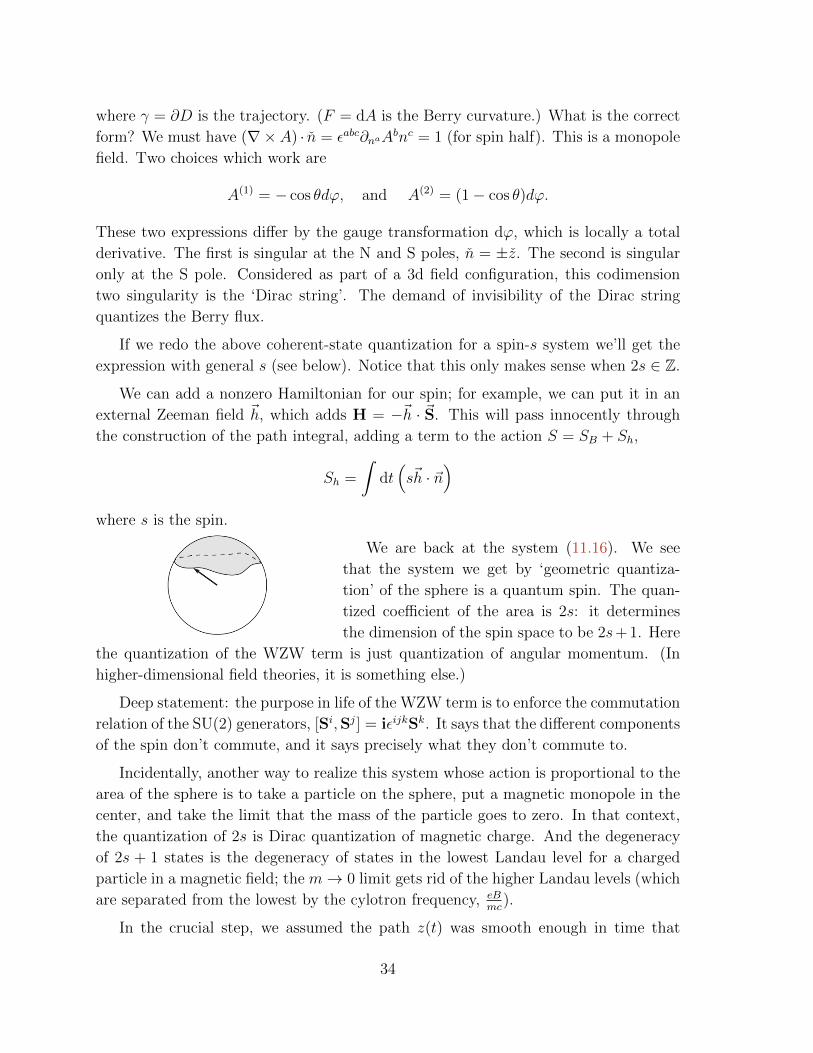
We can add a nonzero Hamiltonian for our spin; for example, we can put it in an
external Zeeman field ~h, which adds H = −~h · ~S. This will pass innocently through
the construction of the path integral, adding a term to the action S = SB + Sh,
Sh =
∫dt(s~h · ~n
)where s is the spin.
We are back at the system (11.16). We see
that the system we get by ‘geometric quantiza-
tion’ of the sphere is a quantum spin. The quan-
tized coefficient of the area is 2s: it determines
the dimension of the spin space to be 2s+ 1. Here
the quantization of the WZW term is just quantization of angular momentum. (In
higher-dimensional field theories, it is something else.)
Deep statement: the purpose in life of the WZW term is to enforce the commutation
relation of the SU(2) generators, [Si,Sj] = iεijkSk. It says that the different components
of the spin don’t commute, and it says precisely what they don’t commute to.
Incidentally, another way to realize this system whose action is proportional to the
area of the sphere is to take a particle on the sphere, put a magnetic monopole in the
center, and take the limit that the mass of the particle goes to zero. In that context,
the quantization of 2s is Dirac quantization of magnetic charge. And the degeneracy
of 2s + 1 states is the degeneracy of states in the lowest Landau level for a charged
particle in a magnetic field; the m→ 0 limit gets rid of the higher Landau levels (which
are separated from the lowest by the cylotron frequency, eBmc
).
In the crucial step, we assumed the path z(t) was smooth enough in time that
34
we could do calculus, z(t + ε) − z(t) = εz(t) + O(ε2). Is this true of the important
contributions to the path integral? Sometimes not, and we’ll come back to this later.
Digression on s > 12. [Auerbach, Interacting Electrons and Quantum Magnetism]
I want to say something about larger-spin representations of SU(2), partly to verify
the claim above that it results in a factor of 2s in front of the Berry phase term. Also,
large s allows us to approximate the integral by stationary phase.
In general, a useful way to think about the coherent state |n〉 is to start with the
maximal-spin eigenstate |s, s〉 of Sz (the analog of spin up for general s), and rotate it
by the rotation that takes Sz to S · n:
|n〉 = R(χ, θ, ϕ) |s, s〉 = eiSzϕeiSyθeiSzψ |s, s〉 = eisψeiSzϕeiSyθ |s, s〉 .
Schwinger bosons. The following is a helpful device for spin matrix elements.
Consider two copies of the harmonic oscillator algebra, with modes a, b satisfing [a, a†] =
1 = [b, b†], [a, b] = [a, b†] = 0. Then
S+ = a†b, S− = b†a, Sz = a†a− b†b
satisfy the SU(2) algebra. The no-boson state |0〉 is a singlet of this SU(2), and the
one-boson states
(a† |0〉b† |0〉
)form a spin-half doublet.
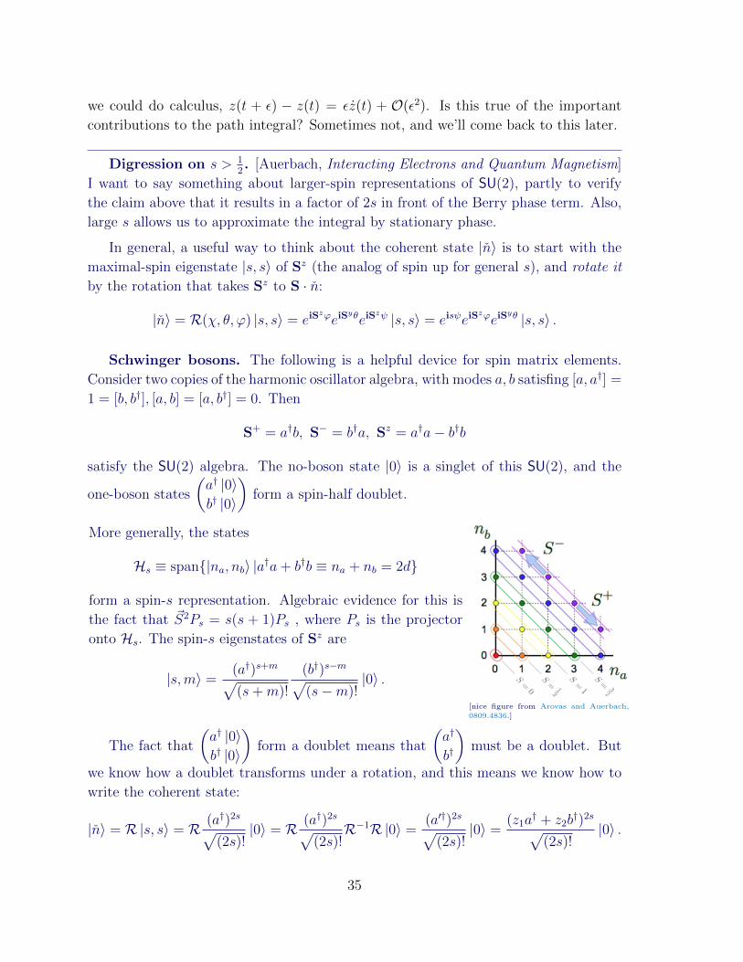
More generally, the states
Hs ≡ span|na, nb〉 |a†a+ b†b ≡ na + nb = 2d
form a spin-s representation. Algebraic evidence for this is
the fact that ~S2Ps = s(s + 1)Ps , where Ps is the projector
onto Hs. The spin-s eigenstates of Sz are
|s,m〉 =(a†)s+m√(s+m)!
(b†)s−m√(s−m)!
|0〉 .
[nice figure from Arovas and Auerbach,
0809.4836.]
The fact that
(a† |0〉b† |0〉
)form a doublet means that
(a†
b†
)must be a doublet. But
we know how a doublet transforms under a rotation, and this means we know how to
write the coherent state:
|n〉 = R|s, s〉 = R (a†)2s√(2s)!
|0〉 = R (a†)2s√(2s)!
R−1R|0〉 =(a′†)2s√
(2s)!|0〉 =
(z1a† + z2b
†)2s√(2s)!
|0〉 .
35

Here
(z1
z2
)=
(eiϕ/2 cos θ
2eiψ/2
e−iϕ/2 sin θ2eiψ/2
)as above9.
But now we can compute the crucial ingredient in the coherent state path integral,
the overlap of successive coherent states:
〈n|n′〉 =e−is(ψ−ψ′)
(2s)!〈0| (z?1a+ z?2b)
2s(z′1a† + z′2b
†)2s |0〉︸ ︷︷ ︸Wick
= (2s)!([z?1a+z?2b,z′1a†+z′2b
†])2s
= e−is(ψ−ψ′)(z?1z′1+z?2z
′2)2s =
(e−i(ψ−ψ′)/2z† · z′
)2s
.
Here’s the point: this is the same as the spin-half answer, raised to the 2s power.
This means that the Berry phase just gets multiplied by 2s, S(s)B [n] = 2sS
( 12)
B [n], as we
claimed.
Semi-classical spectrum. Above we found a path integral representation for the
Green’s function of a spin as a function of time, G(nt, n0; t). The information this con-
tains about the spectrum of the hamiltonian can be extracted by Fourier transforming
G(nt, n0;E) ≡ −i
∫ ∞0
dtG(nt, n0; t)ei(E+iε)t
and taking the trace
Γ(E) ≡∫d2n0
2πG(n0, n0;E) = tr
1
E −H + iε.
This function has poles at the eigenvalues of H. Its imaginary part is the spectral
density, ρ(E) = 1πImΓ(E) =
∑α δ(E − Eα).
The path integral representation is
Γ(E) = −i
∫dt
∮Dn ei((E+iε)t+sS[n]).
The∮
indicates periodic boundary conditions, n(0) = n(t), and S[n] = SB[n] −∫ tdt′Hcl[n]/s. Here Hcl[n] ≡ 〈n|H |n〉.
At large s, field configurations which vary too much in time are cancelled out by the
rapidly oscillating phase, that is: we can try to do these integrals by stationary phase.
The stationarity condition for the n integral is the equations of motion 0 = n×n−∂nHcl.
If H = ~h·S, this gives the Landau-Lifshitz equation (11.17) for precession. We keep only
solutions periodic with t = nT an integer multiple of the period T . The stationarity
condition for the t integral is
0 = E + ∂tS[n] = E −Hcl[n].
9Sometimes (such as in lecture) you may see the notation z1 ≡ u, z2 ≡ v.
36
In the second equality we used the fact that the Berry phase is geometric, it depends
only on the trajectory, not on t (how long it takes to get there). So the semiclassical
trajectories are periodic solutions to the EOM with energy E = Hcl[nE]. The exponent
evaluated on such a trajectory is then just the Berry term. Denoting by nE1 such
trajectories which traverse once (‘prime’ orbits),
Γ(E) ∼∑nE1
∞∑n=0
einsSB [n] =∑nE1
einsSB [n]
1− einsSB [n].
This is an instance of the Gutzwiller trace formula. The locations of poles of this func-
tion approximate the eigenvalues of H. They occur at E = Emsc such that SB[~nEm ] =
2πms. The actual eigenvalues are Em = Em
sc +O(1/s).
If the path integral in question were a 1d particle in a potential, with SB =∫pdx,
and Hcl = p2 + V (x), the semiclassical condition would reduce to
2πm =
∮xEm
p(x)dx =
∫turning points
√Em − V (x)
the Bohr-Sommerfeld condition.
[End of Lecture 45]
11.3.2 Ferromagnets and antiferromagnets.
[Zee §6.5] Now we’ll try D ≥ 1 + 1. Consider a chain of spins, each of spin s ∈ Z/2,
interacting via the Heisenberg hamiltonian:
H =∑j
J~Sj · ~Sj+1.
This hamiltonian is invariant under global spin rotations, Saj → RSajR−1 = RabS
bj for
all j. For J < 0, this interaction is ferromagnetic, so it favors a state like⟨~Sj
⟩= sz.
For J > 0, the neighboring spins want to anti-align; this is an antiferromagnet:⟨~Sj
⟩=
(−1)jsz. Note that I am lying about there being spontaneous breaking of a continuous
symmetry in 1+1 dimensions. Really there is only short-range order because of the
Coleman-Mermin-Wagner theorem. But that is enough for the calculation we want to
do.10
10Even more generally, the consequence of short-range interactions of some particular sign for the
groundstate is not so obvious. For example, antiferromagnetic interactions may be frustrated: If I
want to disagree with both Kenenisa and Lasse, and Kenenisa and Lasse want to disagree with each
other, then some of us will have to agree, or maybe someone has to withhold their opinion, 〈S〉 = 0.
37
We can write down the action that we get by coherent-state quantization – it’s just
many copies of the above, where each spin plays the role of the external magnetic field
for its neighbors:
L = is∑j
z†j∂tzj − Js2∑j
~nj · ~nj+1.
Spin waves in ferromagnets. Let’s use this to find the equation of motion for
small fluctuations δ~ni = ~Si − sz about the ferromagnetic state. Once we recognize
the existence of the Berry phase term, this is the easy case. In fact the discussion is
not restricted to D = 1 + 1. Assume the system is translation invariant, so we should
Fourier transform. The condition that ~n2j = 1 means that δnz(k) = 0.11 Linearizing in
δ~n (using (11.18)) and fourier transforming, we find
0 =
(h(k) − i
2ω
i2ω h(k)
)(δnx(k)
δny(k)
)with h(k) determined by the exchange (J) term. It is the lattice laplacian in k-
space. For example for the square lattice, it is h(k) = 4s|J | (2− cos kxa− cos kya)k→0'
2s|J |a2k2, with a the lattice spacing. For small k, the eigenvectors have ω ∼ k2, a
z = 2 dispersion (meaning that there is scale invariance near ω = k = 0, but space
and time scale differently: k → λk, ω → λ2ω. The two spin polarizations have their
relative phases locked δnx(k) = iδny(k)/hk, and so these modes describe precession
of the spin about the ordering vector. These low-lying spin excitations are visible in
neutron scattering and they dominate the low-temperature thermodynamics. Their
thermal excitations produce a version of the blackbody spectrum with z = 2. We can
determine the generalization of the Stefan-Boltzmann law by dimensional analysis: the
free energy (or the energy itself) is extensive, so F ∝ Ld, but it must have dimensions
of energy, and the only other scale available is the temperature. With z 6= 1, temper-
ature scales like [T ] = [L−z]. Therefore F = cLdTd+1z . (For z = 1 this is the ordinary
Stefan-Boltzmann law).
Notice that a ferromagnet is a bit special because the order parameter Qz =∑
i Szi
is actually conserved, [Qz,H] = 0. This is actually what’s responsible for the funny
z = 2 dispersion of the goldstones, and the fact that although the groundstate breaks
two generators Qx and Qy, there is only one gapless mode. If you are impatient to
understand this connection, take a look at this paper.
111 = n2j∀j =⇒ nj · δnj = 0,∀j which means that for any k,
0 =∑j
eikjanj · δnj =∑q
nz(k − q)δnz(q) = δnzk.
38
Antiferromagnets. [Fradkin, 2d ed, p. 203] Now, let’s study instead the equation
of motion for small fluctuations about the antiferromagnetic state. The conclusion will
be that there is a linear dispersion relation. This would be the conclusion we came
to if we simply erased the WZW/Berry phase term and replaced it with an ordinary
kinetic term1
2g2
∑j
∂t~nj · ∂t~nj .
How this comes about is actually a bit more involved! An important role will be
played12 by the ferromagnetic fluctuation ~j in
~nj = (−1)j ~mj + a~j .
~mj is the AF fluctuation; a is the lattice spacing; s ∈ Z/2 is the spin. The constraint
~n2 = 1 tells us that ~m2 = 1 and ~m · ~= 0.
Why do we have to include both variables? Because ~m are the AF order-parameter
fluctuations, but the total spin is conserved, and therefore its local fluctuations ~ still
constitute a slow mode. This is an illustration of a general point: amongst the low-
energy modes in our effective field theory, we should make sure we keep track of the
conserved quantities, which can often move around but can never disappear. The name
for this principle is hydrodynamics.
The exchange (J) term in the action is (using ~n2r−~n2r−1 ≈ a (∂x ~m2r + 2`2r)+O(a2))
SJ [~nj = (−1)j ~mj + a~j] = −aJs2
∫dxdt
(1
2(∂x ~m)2 + 2`2
).
The WZW terms evaluate to13
SW = sN∑j=1
W0[(−1)jmj+`j]N→∞,a→0,Na fixed
'∫
dxdt(s
2~m · (∂t ~m× ∂x ~m) + s~ · (~m× ∂t ~m)
).
12A pointer to the future: this story is very similar to the origin of the second order kinetic term for
the Goldstone mode in a superfluid arises. The role of ~ there is played by ρ, the density. Naturally,
we will discuss this when we do coherent state quantization of bosons in §11.5.13The essential ingredient is
δW0[n] =
∫dtδ~n · (~n× ∂t~n) .
So
W0[n2r]−W [n2r−1] = −1
2
dx
a
δW0
δni∂xn
ia = −1
2dxn× ∂tn · ∂xn.
39
Altogether, we find that ` is an auxiliary field with no time derivative:
L[m, `] = −2aJs2~2 + s~ · (~m× ∂t ~m) + L[m]
so we can integrate out ` (this is the step analogous to what we’ll do for ρ in the EFT
of SF in §11.5) to find
S[~m] =
∫dxdt
(1
2g2
(1
vs(∂t ~m)2 − vs (∂x ~m)2
)+
θ
8πεµν ~m · (∂µ ~m× ∂ν ~m)
), (11.24)
with g2 = 2s
and vs = 2aJs, and θ = 2πs. The equation of motion for small fluctuations
of ~m therefore gives linear dispersion with velocity vs. Notice that there are two
independent gapless modes. Some of these fluctuations have wavenumber k close to
π, since they are fluctuations of the AF order (k = π means changing sign between
each site), that is, ω ∼ |k − π|. (For a more microscopic treatment, see the book by
Auerbach.)
The last (‘theta’) term in (11.24) is a total derivative. This means it doesn’t affect
the EOM, and it doesn’t affect the Feynman rules. It is even more topological than
the WZW term – its value only depends on the topology of the field configuration,
and not on local variations. It is like the θF ∧ F term in 4d gauge theory. You might
think then that it doesn’t matter. Although it doesn’t affect small fluctuations of the
fields, it does affect the path integral. Where have we seen this functional before? The
integrand is the same as in our 2d representation of the WZW term in 0+1 dimensions:
the object multiplying theta counts the winding number of the field configuration ~m,
the number of times Q the map ~m : R2 → S2 covers its image (we can assume that the
map ~m(|x| → ∞) approaches a constant, say the north pole). We can break up the
path integral into sectors, labelled by this number Q ≡ 18π
∫dxdt εµν ~m · (∂µ ~m× ∂ν ~m) :
Z =
∫[D~m]eiS =
∑Q∈Z
∫[D~m]Qe
iSθ=0eiθQ .
θ determines the relative phase of different topological sectors (for θ = π, this a minus
sign for odd Q).
Actually, the theta term makes a huge difference. (Perhaps it is not so surprising
if you think about the quantum mechanics of a particle constrained to move on a ring
with magnetic flux through it?) The model with even s flows to a trivial theory in the
IR, while the model with odd s flows to a nontrivial fixed point, called the SU(2)1 WZW
model. It can be described in terms of one free relativistic boson. If you are impatient
to understand more about this, the 2nd edition of the book by Fradkin continues this
discussion. Perhaps I can be persuaded to say more.
[End of Lecture 46]
40
Nonlinear sigma models in perturbation theory. Let us discuss what happens
in perturbation theory in small g. A momentum-shell calculation integrating out fast
modes (see the next subsection, §11.3.3) shows that
dg2
d`= (D − 2)g2 + (n− 2)KDg
4 +O(g3) (11.25)
where ` is the logarithmic RG time, and `→∞ is the IR. n is the number of components
of n, here n = 3, and KD = ΩD−1
(2π)Das usual. Cultural remark: the second term
is proportional to the curvature of the target space, here Sn−1, which has positive
curvature for n > 1. For n = 2, we get S1 which is one-dimensional and hence flat and
there is no perturbative beta function. In fact, for n = 2, it’s a free massless scalar.
(But there is more to say about this innocent-looking scalar!)
The fact that the RHS of (11.25) is positive in D = 2 says that this model is
asymptotically free – the coupling is weak in the UV (though this isn’t so important if
we are starting from a lattice model) and becomes strong in the IR. This is opposite
what happens in QED; the screening of the charge in QED makes sense in terms of
polarization of the vacuum by virtual charges. Why does this antiscreening happen
here? There’s a nice answer: the effect of the short-wavelength fluctuations is to make
the spin-ordering vector ~n effectively smaller. It is like what happens when you do
the block spin procedure, only this time don’t use majority rule, but just average the
spins. But rescaling the variable ~n → a~n with a <∼ 1 is the same as rescaling the
coupling g → g/a – the coupling gets bigger. (Beware Peskin’s comments about the
connection between this result and the Coleman-Mermin-Wagner theorem: it’s true
that the logs in 2d enhance this effect, but in fact the model can reach a fixed point at
finite coupling; in fact, this is what happens when θ = π.)
Beyond perturbation theory. Like in QCD, this infrared slavery (the dark side
of asymptotic freedom) means that we don’t really know what happens in the IR from
this calculation. From other viewpoints (Bethe ansatz solutions, many other methods),
we know that (for integer s) there is an energy gap above the groundstate (named after
Haldane) of order
ΛH ∼ Λ0e− c
g20 ,
analogous to the QCD scale. Here g0 is the value of g at the scale Λ0; so ΛH is roughly
the energy scale where g becomes large. This is dimensional transmutation again.
For s ∈ Z, for studying bulk properties like the energy gap, we can ignore the theta
term since it only appears as e2πin, with n ∈ Z in the path integral. 14 For half-integer
14θ = 2πn does, however, affect other properties, such as the groundstate wavefunction and the
behavior in the presence of a boundary. θ = 2π is actually a different phase of matter than θ = 0.
It is an example of a SPT (symmetry-protected topological) phase, the first one discovered. See the
homework for more on this.
41
s, there is destructive interference between the topological sectors. Various results
(such as the paper by Read and Shankar, Nuclear Physics B336 (1990) 457-474, which
contains an amazingly apt Woody Allen joke) show that this destroys the gap. This last
sentence was a bit unsatisfying; more satisfying would be to understand the origin of
the gap in the θ = 2πn case, and show that this interference removes that mechanism.
This strategy is taken in this paper by Affleck.
11.3.3 The beta function for 2d non-linear sigma models
[Polyakov §3.2; Peskin §13.3; Auerbach chapter 13] I can’t resist explaining the result
(11.25). Consider this action for a D = 2 non-linear sigma model with target space
Sn+1, of radius R:
S =
∫d2xR2∂µn · ∂µn ≡
∫d2xR2dn2.
Notice that R is a coupling constant (it’s what I called 1/g earlier). In the second step
I made some compact notation.
Since not all of the components of n are independent (recall that n · n = 1!),
the expansion into slow and fast modes here is a little trickier than in our previous
examples. Following Polyakov, let
ni(x) ≡ ni<(x)√
1− φ2> +
n−1∑a=1
φ>a (x)eia(x). (11.26)
Here the slow modes are represented by the unit vector ni<(x), n< ·n< = 1; the variables
eia are a basis of unit vectors spanning the n− 1 directions perpendicular to ~n<(x)
n< · ea = 0, ea · ea = 1; (11.27)
they are not dynamical variables and how we choose them does not matter.
The fast modes are encoded in φ>a (x) ≡∫ Λ
Λ/sdkeikxφk, which only has fourier modes
in a shell of momenta, and φ2> ≡
∑n−1a=1 φ
>a φ
>a . Notice that differentiating the relations
in (11.27) gives
n< · dn< = 0, n< · dea + dn< · ea = 0. (11.28)
Below when I write φs, the > symbol is implicit.
We need to plug the expansion (11.26) into the action, whose basic ingredient is
dni = dni<(1− φ2
) 12 − ni<
φ · dφ√1− φ2
+ dφ · ei + φ · dei.
42
So Seff =∫d2x L with
L =1
2g2(d~n)2
=1
2g2
(dn<)2 (1− φ2)
+ dφ2︸︷︷︸kinetic term for φ
+2φadφb~ea · d~eb
+ dφad~n< · ~ea︸ ︷︷ ︸source for φ
+φaφbd~ea · d~eb +O(φ3)
(11.29)
So let’s do the integral over φ, by treating the dφ2 term as the kinetic term in a gaussian
integral, and the rest as perturbations:
e−Seff[n<] =
∫[Dφ>]ΛΛ/se
−∫L =
∫[Dφ>]ΛΛ/se
− 12g2
∫(dφ)2
(all the rest) ≡ 〈all the rest〉>,0 Z>,0 .
The 〈...〉>,0s that follow are with respect to this measure.
=⇒ Leff[n<] =1
2g2(dn<)2
(1−
⟨φ2⟩>,0
)+〈φaφb〉>,0 d~ea·d~eb+terms with more derivatives
〈φaφb〉>,0 = δabg2
∫ Λ
Λ/s
d2k
k2= g2K2 log(s)δab, K2 =
1
2π.
What to do with this d~ea · d~eb nonsense? Remember, ~ea are just some arbitrary
basis of the space perpendicular to n<; its variation can be expanded in our ON basis
at x, (n<, ec) as
d~ea = (dea · n<) n< +n−1∑c=1
(d~ea · ~ec)︸ ︷︷ ︸(11.28)
= −dn<·~ea
~ec
Therefore
d~ea · d~ea = + (dn<)2 +∑c,a
(~ec · d~ea)2
where the second term is a higher-derivative operator that we can ignore for our present
purposes. Therefore
Leff[n] =1
2g2(dn<)2 (1− ((N − 1)− 1) g2K2 log s
)+ ...
' 1
2
(g2 +
g4
4π(N − 2) log s+ ...
)−1
(dn<)2 + ... (11.30)
Differentiating this running coupling with respect to s gives the one-loop term in
the beta function quoted above. The tree-level (order g2) term comes from engineering
dimensions.
43
11.3.4 CP1 representation and Large-N
[Auerbach, Interacting Electrons and Quantum Magnetism, Polyakov, Gauge fields and
strings] Above we used large spin as our small parameter to try to control the con-
tributions to the path integral. Here we describe another route to a small parameter,
which can be just as useful if we’re interested in small spin (like spin-12).
Recall the relationship between the coherent state vector n and the spinor compo-
nents z: na = z†σaz. Imagine doing this at each point in space and time:
na(x) = z†(x)σaz(x). (11.31)
We saw that the Berry phase term could be written nicely in terms of z as iz†z, what
about the rest of the path integral?
First, some counting: 1 = n2 ⇔ 1 = z† · z =∑
m=↑,↓ |zm|2. But this leaves only two
components of n, and three components of zm. The difference is made up by the fact
that the rephasing
zm(x)→ eiχ(x)zm(x) (11.32)
doesn’t change n. So it can’t act on the physical Hilbert space. This is a (local, since
χ(x) depends on x) U(1) gauge redundancy of the description in terms of z.
There two ways to proceed from here. One is via exact path integral tricks which
are relatively straightforward in this case, but generally unavailable. The second is by
the Landau method of knowing the answer: what else could it be.
Path integral manipulations. [Auerbach, chapter 14] First notice that the AF
kinetic term is
∂µna∂µna = 4
(∂µz
†∂µz −AµAµ)
= 4(∂µz
†∂µz −AµAµz†z). (11.33)
where Aµ ≡ − i2
(z†∂µz − ∂µz†z
)is a connection one-form made from z itself. Notice
that Aµ → Aµ−∂χ and the BHS of (11.33) is gauge invariant under (11.32). We must
impose the constraint |z(x)|2 = 1 at each site, which let’s do it by a lagrange muliptlier
δ[|z|2 − 1] =∫Dλ ei
∫ddxλ(x)(|z|2−1). In the action, the A2 term is a self-interaction of
the zs, which makes it difficult to do the integral. The standard trick for ameliorating
this problem is the Hubbard-Stratonovich identity:
ecA2µ =
√c
π
∫dAµ e
−cA2µ+2cAµAµ .
The saddle point value of A is A. This gives
e−#∫dn2
=
∫[dA]e−#
∫|(∂−iA)z|2 .
44
Finally, let’s think about the measure at each point:∫d2nδ(n2−1)... =
∫ π0
sin θdθ∫ 2π
0dϕ....
Compare this to the integral over zs, parametrized as z =
(ρ1e
iφ1
ρ2eiφ2
)=
(cos θ
2eiϕ/2eiχ/2
sin θ2e−iϕ/2eiχ/2
):
∫dzdz†δ(|z|2 − 1)... =
∫ ∏m=1,2
ρmdρmdφmδ(ρ1 + ρ2 − 1)...
= c
∫dρρ√
1− ρ2dϕdχ... = c′∫
sinθ
2cos
θ
2dθdϕdχ...
which is the same as∫dn except for the extra integral over χ: that’s the gauge di-
rection. The integral over χ is just a number at each point, as long as we integrate
invariant objects (otherwise, it gives zero). Thinking of z as parametrizing an arbitrary
normalized spinor z = R(θ, ϕ, χ)
(1
0
), so thatR is an arbitrary element of SU(2), we’ve
just shown the geometric equivalence between the round S2 and CP1 = SU(2)/U(1).
ZS2 '∫
[dzdz†dAdλ]e−∫dDx
(2ΛD−2
g2|(∂−iA)z|2−λ(|z|2−1)
). (11.34)
This is a U(1) gauge theory with N = 2 charged scalars. It is called the CP1 sigma
model. There are two slightly funny things: (1) the first is that the gauge field A lacks a
kinetic term: in the microscopic description we are making here, it is infinitely strongly
coupled. We’ll see what the interactions with matter have to say about the coupling
in the IR. (2) The second funny thing is that the scalars z have a funny interaction
with this field λ which only appears linearly. If we add a λ2/κ quadratic term, we can
do the lambda integral and find V (|z|2) = κ(|z|2 − 1)2, an ordinary quartic potential
for |z|. This has the effect of replacing the delta function imposition with an energetic
recommendation that |z|2 = 1. This is called a soft constraint, and it shouldn’t change
the universal physics.
Alternatively, we could have arrived at this point
ZS2 '∫
[dzdz†dA]e−∫dDx
(2ΛD−2
g2|(∂−iA)z|2−κ(|z|2−1)
2)
by regarding (11.31) as a slave-particle or parton ansatz for a new set of variables.
The demand of gauge invariance (11.32) is a strong constraint on the form of the
interactions, and requires the inclusion of the gauge field A.
Other such ansatze are possible, such as one in terms of slave fermions ~S = ψ†~σψ.
In this case, this turns out to be also correct. (More later, after we discuss anomalies.)
More generally, any given ansatz may not be useful to describe the relevant physics.
[End of Lecture 47]
45
Large N . This representation allows the introduction of another possible small
parameter, namely the number of components of z. Suppose instead of two components,
it has NN∑m=1
|zm|2 =N
2,
and let’s think about the resulting CPN−1 sigma model (notice that CPN−1 and SN
are different generalizations of S2, in the sense that for N → 1 they are both S2):
ZCPN−1 =
∫[dzdz†dAdλ]e
−∫dDx
(2ΛD−2
g2|(∂−iA)z|2−λ(|z|2−N/2)
)
=
∫[dAdλ]e−NS[A,λ] N1' Z ′e−NS[A,λ].
The z-integral is gaussian in the representation (11.34) even forN = 2, but the resulting
integrals over A, λ are then horrible, with action
S[A, λ] = tr ln(− (∂ − iA)2 + λ
)− iΛD−2
g2
∫λ.
The role of large N is to make those integrals well-peaked about their saddle point.
The saddle point equations are solved by A = 0 (though there may sometimes be other
saddles where A 6= 0, which break various discrete symmetries). This leaves us with
S[0, λ] =
∫dDk ln(k2 + λ)− i
g2V λ
(where V is the number of sites, the volume of space, and I’ve assumed constant λ),
which is solved by λ = −iλ satisfying∫dDk
k2 + λ=
1
g2.
The solution of this equation depends on the number of dimensions D.
D = 1 :1
g2Λ=
∫dk
k2 + λ=
1√λ
∫dk
k2 + 1=⇒ λ = g4Λ2 .
This says that the mass of the excitations is m = g2. Where did that come from?
D = 1 means we are studying the quantum mechanics of a particle contrained to move
on CPN−1:
H =1
2g2Λ∂z∂z +
(|z|2 −N/2
)2.
The groundstate is the uniform state 〈z|groundstate〉 = Ψ(z) = 1vol
. QM of finite
number of degrees of freedom on a compact space has a gap above the groundstate.
This gap is determined by the kinetic energy and naturally goes like g2Λ.
46
D = 2 : g−2 =
∫d2k
k2 + λ= − 1
4πln
λ
Λ2=⇒ λ = Λ2e
− 4πg2 .
This is the case with asymptotic freedom; here we see again that asymptotic freedom
is accompanied by dimensional transmutation: the interactions have generated a mass
scale
m = Λe− 2πg2
which is parametrically (in the bare coupling g) smaller than the cutoff.
D = 3 :Λ
g2=
∫d3k
k2 + λ=⇒ |
√λ| = Λ
2
(2
π− 4π
g2
).
Notice that for D ≥ 3 there is a critical value of g below which there is no solution.
That means symmetry breaking: the saddle point is at λ = m2 = 0, and the z-fields
are gapless Goldstone modes. This doesn’t happen in D ≤ 2. The critical coupling
occurs when g−2c =
∫dDkk2 ' ΛD−2
D−2. The rate at which the mass goes to zero as g → gc
from above is
m2 ' Λ2
(g2 − g2
c
g2c
) 2D−2
.
This is a universal exponent. (For more on critical exponents from large-N calculations,
see Peskin p. 464-465.)
A quantity we’d like to be able to compute for N = 2 is S+−(x) ≡ 〈S+(0)S−(x)〉.We can write this in terms of the coherent state variables using the identity
Sa = Ns∫dn |n〉 〈n|na, (Ns =
(s+ 1)(2s+ 1)
4π).
(Up to the constant factor, this identity follows from SU(2) invariance. The constant
can be checked by looking at a convenient matrix element of the BHS.) Then:
S+−(x) = 〈(nx + iny)(0)(nx − iny)(x)〉 .
Recalling that nx + iny = z†σ+z = z?1z2, we can generalize this to large N as the
four-point function
Sm6=m′(x) = 〈z?m(0)zm′(0)z?m(x)zm′(x)〉 N1' |G(x)|2
which factorizes at leading order in large N . This phenomenon (large-N factorization)
that at large-N the correlations are dominated by the disconnected bits is general. (Let
me postpone the diagrammatic argument for a bit.) The factors are:
G(x) =1
Z
∫[dz]z†(0)z(x)e
− 2Λd−2
g2
∫ddk(|k|2+λ)z†kzk−
NV Λd−2
g2λ
47
=
∫ddk
e−ikx
|k|2 + λ' 1
|x| d−12
e−|x|√λ.
This says that the correlation length for the spins in Sm6=m′(x)
x>ξ' 1|x|d−1 e
−ξ|x| is ξ = 1
2√λ
depends variously on d. In D = 1, it is ξ = Λ/g2, so large-N predicts a gap, growing
with g. In D = 2, the correlation length is ξ = Λ−1e+ 2πg2 In D = 3, the correlation
length diverges as g → gc ξ = Λ−1(
2π− 4π
g2
)−1
, signaling the presence of gapless modes,
which we interpret as Goldstones.
Exercise. Check that the other components of the spin such as Sz = |zm|2−|zm′ |2have the same falloff, as they must by SU(N) symmetry.
A dynamical gauge field emerges. Finally, let me show you that a gauge field
emerges. Let’s expand the action Seff[A, λ] about the saddle point at A = 0, λ = λ ≡m2:
S[A = 0 + a, λ = m2 + v] = W0 + W0︸︷︷︸=0by def
+W2 +O(δ3)
where the interesting bit is the terms quadratic in the fluctuations:
W2 =N
2
∫dDq (v(q)Π(q)v(−q) + Aµ(q)Πµν(q)Aν(−q))
where
Π(q) = ... =
∫dDk
1
(k2 +m2)((k + q)2 +m2)(11.35)
Πµν = +diamagnetic diagram =
∫dDk
(2k + q)µ(2k + q)ν(k2 +m2)((k + q)2 +m2)
−2gµν
∫dDk
k2 +m2.
(11.36)
Familiarly, gauge invariance implies that qµΠµν(q) = 0 – it prevents a mass for the
gauge field. For example, in D = 2, the long wavelength behavior is
Πµν(q)q→0∼ c
m2
(q2gµν − qµqν
)which means that the effective action for the gauge fluctuation is
W2 ∼N
m2
∫d2xFµνF
µν + more derivatives.
It is a dynamical gauge field.
Another term we can add to the action for a 2d gauge field is
θ
∫F
2π
48

where we regard F = dA as a two-form. This is the 2d theta term, analogous to∫F ∧ F in D = 4 in that F = dA is locally a total derivative, it doesn’t affect the
equations of motion, and it integrates to an integer on smooth configurations (we will
show this when we study anomalies). This integer is called the Chern number of the
gauge field configuration. What integer is it? On the homework you’ll show that
F ∝ εabcnadnbdnc. It’s the skyrmion number! So the coefficient is θ = 2πs.
11.3.5 Large-N diagrams.
I think it will help to bring home some of the previous ideas by rederiving them using
diagrams in a familiar context. So let’s study the O(N) model:
L =1
2∂~ϕ · ∂~ϕ+
g
4N(~ϕ · ~ϕ)2 +
m2
2~ϕ · ~ϕ. (11.37)
Let’s do euclidean spacetime, D dimensions. The bare propagator is
〈ϕb(x)ϕa(0)〉 =
∫dDk
e−ikx
k2 +m2≡∫
dDk ∆0(k).
The bare vertex is −2gN
(δabδcd + δacδbd + δadδbc). With this normalization, the leading
correction to the propagator is
= − g
4N(4N + 8)δab
∫dq
q2 +m2
N1' −gδab∫
dq∆0(q)
of order N0. This is the motivation for the normalization of the coupling in (11.37).
Which diagrams dominate at large N (and fixed g)? Compare two diagrams at
the same order in λ with different topology of the index flow: eyeball and
cactus . The former has one index loop, and the latter has two, and therefore
dominates. The general pattern is that: at large N cacti dominate the 1PI self-energy.
Each extra pod we add to the cactus costs a factor of g/N but gains an index loop N .
So the sum of cacti is a function of gN0.
The full propagator, by the usual geometric series, is then
∆F (k) =1
k2 +m2 + Σ(k). (11.38)
We can sum all the cacti by noticing that cacti are self-similar: if we replace ∆0 by ∆F
in the propagator:
Σ(p) = g
∫dDk∆F (k) +O(1/N). (11.39)
49
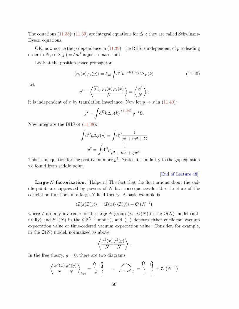
The equations (11.38), (11.39) are integral equations for ∆F ; they are called Schwinger-
Dyson equations,
OK, now notice the p-dependence in (11.39): the RHS is independent of p to leading
order in N , so Σ(p) = δm2 is just a mass shift.
Look at the position-space propagator
〈ϕb(x)ϕa(y)〉 = δab
∫dDke−ik(x−y)∆F (k). (11.40)
Let
y2 ≡⟨∑
a ϕa(x)ϕa(x)
N
⟩=
⟨ϕ2
N
⟩;
it is independent of x by translation invariance. Now let y → x in (11.40):
y2 =
∫dDk∆F (k)
(11.39)= g−1Σ.
Now integrate the BHS of (11.38):∫dDp∆F (p) =
∫dD
1
p2 +m2 + Σ
y2 =
∫dDp
1
p2 +m2 + gy2.
This is an equation for the positive number y2. Notice its similarity to the gap equation
we found from saddle point.
[End of Lecture 48]
Large-N factorization. [Halpern] The fact that the fluctuations about the sad-
dle point are suppressed by powers of N has consequences for the structure of the
correlation functions in a large-N field theory. A basic example is
〈I(x)I(y)〉 = 〈I(x)〉 〈I(y)〉+O(N−1
)where I are any invariants of the large-N group (i.e. O(N) in the O(N) model (nat-
urally) and SU(N) in the CPN−1 model), and 〈...〉 denotes either euclidean vacuum
expectation value or time-ordered vacuum expectation value. Consider, for example,
in the O(N) model, normalized as above⟨ϕ2(x)
N
ϕ2(y)
N
⟩.
In the free theory, g = 0, there are two diagrams⟨ϕ2(x)
N
ϕ2(y)
N
⟩free
= = +O(N−1
)50
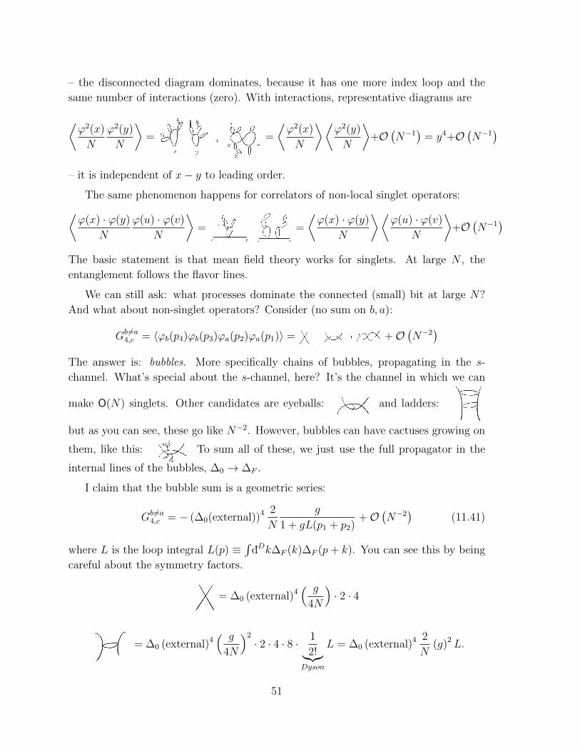
– the disconnected diagram dominates, because it has one more index loop and the
same number of interactions (zero). With interactions, representative diagrams are
⟨ϕ2(x)
N
ϕ2(y)
N
⟩= =
⟨ϕ2(x)
N
⟩⟨ϕ2(y)
N
⟩+O
(N−1
)= y4+O
(N−1
)– it is independent of x− y to leading order.
The same phenomenon happens for correlators of non-local singlet operators:⟨ϕ(x) · ϕ(y)
N
ϕ(u) · ϕ(v)
N
⟩= =
⟨ϕ(x) · ϕ(y)
N
⟩⟨ϕ(u) · ϕ(v)
N
⟩+O
(N−1
)The basic statement is that mean field theory works for singlets. At large N , the
entanglement follows the flavor lines.
We can still ask: what processes dominate the connected (small) bit at large N?
And what about non-singlet operators? Consider (no sum on b, a):
Gb 6=a4,c = 〈ϕb(p4)ϕb(p3)ϕa(p2)ϕa(p1)〉 = +O
(N−2
)The answer is: bubbles. More specifically chains of bubbles, propagating in the s-
channel. What’s special about the s-channel, here? It’s the channel in which we can
make O(N) singlets. Other candidates are eyeballs: and ladders:
but as you can see, these go like N−2. However, bubbles can have cactuses growing on
them, like this: To sum all of these, we just use the full propagator in the
internal lines of the bubbles, ∆0 → ∆F .
I claim that the bubble sum is a geometric series:
Gb6=a4,c = − (∆0(external))4 2
N
g
1 + gL(p1 + p2)+O
(N−2
)(11.41)
where L is the loop integral L(p) ≡∫
dDk∆F (k)∆F (p+ k). You can see this by being
careful about the symmetry factors.
= ∆0 (external)4( g
4N
)· 2 · 4
= ∆0 (external)4( g
4N
)2
· 2 · 4 · 8 · 1
2!︸︷︷︸Dyson
L = ∆0 (external)4 2
N(g)2 L.
51
Similarly, the chain of two bubbles is 2Ng3L2, etc.
Here’s how we knew this had to work without worrying about the damn symmetry
factors: the bubble chain is the σ propagator! At the saddle, σ ' ϕaϕa, which is
what is going in and out of this amplitude. And the effective action for sigma (after
integrating out ϕ) is
Seff[σ] =
∫σ2
g+ tr ln
(∂2 +m2 + σ
).
The connected two-point function means we subract of 〈σ〉 〈σ〉, which is the same as
considering the two point function of the deviation from saddle value. This is
〈σ1σ2〉 =
(δ2
δσ1δσ2
Seff[σ]
)−1
=
(1
g−1 +(
1∂2+m2+σ
)2
)−1
which becomes exactly the expression above if we write it in momentum space.
Two comments: (1) We were pretty brash in integrating out all the ϕ variables and
keeping the σ variable: how do we know which are the slow ones and which are the
fast ones? This sort of non-Wilsonian strategy is common in the literature on large-N ,
where physicists are so excited to see an integral that they can actually do that they
don’t pause to worry about slow and fast. But if we did run afoul of Wilson, at least
we’ll know it, because the action for σ will be nonlocal.
(2) σ ∼ ϕ2 is a composite operator. Nevertheless, the sigma propagator we’ve just
derived can have poles at some p2 = m2 (likely with complex m). These would produce
particle-like resonances in a scattering experiment (such as 2−2 scattering of ϕs of the
same flavor) which involved sigmas propagating in the s-channel. Who is to say what
is fundamental.
Now that you believe me, look again at (11.41); it is of the form
Gb 6=a4,c = − (∆0(external))4 2
Ngeff(p1 + p2) +O
(N−2
)where now
geff(p) =g
1 + g∫
dDk∆F (k)∆F (p+ k))
is a momentum-dependent effective coupling, just like one dreams of when talking
about the RG.
52
11.4 Coherent state path integrals for fermions
We’ll need these for our discussion of anomalies, and if we ever get to perturbative
QCD (which differs from Yang-Mills theory by the addition of fermionic quarks).
[Shankar, Principles of QM, path integrals revisited. In this chapter of his great
QM textbook, Shankar sneaks in lots of insights useful for modern condensed matter
physics]
Consider the algebra of a single fermion mode operator15:
c, c = 0, c†, c† = 0, c, c† = 1 .
With a single mode, the general Hamiltonian is
H = c†c (ω0 − µ)
(ω0 and µ are (redundant when there is only one mode) constants). This algebra is
represented on a two-state system |1〉 = c† |0〉. We might be interested in its thermal
partition function
Z = tr e−HT .
(In this example, it happens to equal Z = 1 + e−ω0−µT , as you can see by computing the
trace in the eigenbasis of n = c†c. But never mind that; the one mode is a proxy for
many, where it’s not quite so easy to sum.) How do we trotterize this? That is, what
is ‘the’ corresponding classical system? (One answer is to use the (0d) Jordan-Wigner
map which relates spins and fermions. Perhaps more about that later. Here’s another,
different, answer.) We can do the Trotterizing using any resolution of the identity on
H, so there can be many very-different-looking answers to this question.
Let’s define coherent states for fermionic operators:
c |ψ〉 = ψ |ψ〉 . (11.42)
Here ψ is a c-number (not an operator), but acting twice with c we see that we must
have ψ2 = 0. ψ is a grassmann number. These satisfy
ψ1ψ2 = −ψ2ψ1, ψc = −cψ (11.43)
– they anticommute with each other and with fermionic operators, and commute with
ordinary numbers and bosons. They seem weird but they are easy. We’ll need to
15For many modes,
ci, cj = 0, c†j , c†j = 0, cj , c†j = 1δij .
53
consider multiple grassmann numbers when we have more than one fermion mode,
where c1, c2 = 0 will require that they anticommute ψ1, ψ2 = 0 (as in the def-
inition (11.43)); note that we will be simultaneously diagonalizing operators which
anticommute.
The solution to equation (11.42) is very simple:
|ψ〉 = |0〉 − ψ |1〉
where as above |0〉 is the empty state (c |0〉 = 0) and |1〉 = c† |0〉 is the filled state.
(Check: c |ψ〉 = c |0〉 − cψ |1〉 = +ψc |1〉 = ψ |0〉 = ψ |ψ〉 .)
Similarly, the left-eigenvector of the creation operator is⟨ψ∣∣ c† =
⟨ψ∣∣ ψ, ⟨
ψ∣∣ = 〈0| − 〈1| ψ = 〈0|+ ψ 〈1| .
Notice that these states are weird in that they are elements of an enlarged hilbert space
with grassmann coefficients (usually we just allow complex numbers). Also, ψ is not
the complex conjugate of ψ and⟨ψ∣∣ is not the adjoint of |ψ〉. Rather, their overlap is⟨
ψ|ψ⟩
= 1 + ψψ = eψψ.
Grassmann calculus summary. In the last expression we have seen an example
of the amazing simplicity of Taylor’s theorem for grassmann functions:
f(ψ) = f0 + f1ψ .
Integration is just as easy and its the same as taking derivatives:∫ψdψ = 1,
∫1dψ = 0.
With more than one grassmann we have to worry about the order:
1 =
∫ψψdψdψ = −
∫ψψdψdψ.
The only integral, really, is the gaussian integral:∫e−aψψdψdψ = a.
Many of these give ∫e−ψ·A·ψdψdψ = detA.
54
Here ψ ·A · ψ ≡(ψ1, · · · , ψM
)A11 A12 · · ·A21
. . . · · ·...
.... . .
ψ1
...
ψM
. One way to get this expression
is to change variables to diagonalize the matrix A.
⟨ψψ⟩≡∫ψψe−aψψdψdψ∫e−aψψdψdψ
= −1
a= −
⟨ψψ⟩.
If for many grassman variables we use the action S =∑
i aiψiψi (diagonalize A
above) then ⟨ψiψj
⟩=δijai≡ 〈ij〉 (11.44)
and Wick’s theorem here is⟨ψiψjψkψl
⟩= 〈il〉 〈jk〉 − 〈ik〉 〈jl〉 .
Back to quantum mechanics: The resolution of 1 in this basis is
1 =
∫dψdψ e−ψψ |ψ〉
⟨ψ∣∣ (11.45)
And if A is a bosonic operator (made of an even number of grassmann operators),
trA =
∫dψdψ e−ψψ
⟨−ψ∣∣A |ψ〉 .
(Note the minus sign; it will lead to a deep statement.) So the partition function is:
Z =
∫dψ0dψ0 e
−ψ0ψ0⟨−ψ0
∣∣ e−HT︸︷︷︸
=(1−∆τH) · · · (1−∆τH)︸ ︷︷ ︸M times
|ψ0〉
Now insert (11.45) in between each pair of Trotter factors to get
Z =
∫ M−1∏l=0
dψldψle−ψlψl
⟨ψl+1
∣∣ (1−∆τH) |ψl〉 .
Because of the −ψ in (11.45), to get this nice expression we had to define an extra
letter
ψM = −ψ0, ψM = −ψ0 (11.46)
so we could replace⟨−ψ0
∣∣ =⟨ψM∣∣. [End of Lecture 49]
55
Now we use the coherent state property to turn the matrix elements into grassmann-
valued functions:⟨ψl+1
∣∣ (1−∆τH(c†, c))|ψl〉 =
⟨ψl+1
∣∣ (1−∆τH(ψl+1, ψl))|ψl〉
∆τ→0= eψl+1ψle−∆τH(ψl+1,ψl).
It was important that in H all cs were to the right of all c†s, i.e. that H was normal
ordered.)
So we have
Z =
∫ M−1∏l=0
dψldψle−ψlψleψl+1ψle−∆τH(ψl+1,ψl)
=
∫ M−1∏l=0
dψldψl exp
∆τ
ψl+1 − ψl∆τ︸ ︷︷ ︸
=∂τ ψ
ψl −H(ψl+1, ψl)
'∫
[DψDψ] exp
(∫ 1/T
0
dτ ψ(τ) (−∂τ − ω0 + µ)ψ(τ)
)=
∫[DψDψ]e−S[ψ,ψ]. (11.47)
Points to note:
• In the penultimate step we defined, as usual, continuum fields
ψ(τl = ∆τ l) ≡ ψl, ψ(τl = ∆τ l) ≡ ψl.
• We elided the difference H(ψl+1, ψl) = H(ψl, ψl) +O(∆τ) in the last expression.
This difference is usually negligible and sometimes helpful (an example where it’s
helpful is the discussion of the number density below).
• The APBCs (11.46) on ψ(τ+ 1T
) = −ψ(τ) mean that in its fourier representation16
ψ(τ) = T∑n
ψ(ω)e−iωnτ , ψ(τ) = T∑n
ψ(ω)eiωnτ (11.48)
the Matsubara frequencies
ωn = (2n+ 1)πT, n ∈ Z
are half-integer multiples of πT .
• The measure [DψDψ] is defined by this equation, just as in the bosonic path
integral.
16ψ is still not the complex conjugate of ψ but the relative sign is convenient.
56
• The derivative of a grassmann function is also defined by this equation; note that
ψl+1 − ψl is not ‘small’ in any sense.
• In the last step we integrated by parts, i.e. relabeled terms in the sum, so∑l
(ψl+1 − ψl
)ψl =
∑l
ψl+1ψl−∑l
ψlψl =∑l′=l−1
ψl′ψl−1−∑l
ψlψl = −∑l
ψl (ψl − ψl−1) .
Note that no grassmanns were moved through each other in this process.
The punchline of this discussion for now is that the euclidean action is
S[ψ, ψ] =
∫dτ(ψ∂τψ +H(ψ, ψ)
).
The first-order kinetic term we’ve found ψ∂τψ is sometimes called a ‘Berry phase term’.
Note the funny-looking sign.
Continuum limit warning (about the red ' in (11.47)). The Berry phase term
is actuallyN−1∑l=0
ψl+1 (ψl+1 − ψl) = T∑ωn
ψ(ωn)(1− eiωnτ
)ψ(ωn)
and in (11.47) we have kept only the leading nonzero term:(1− eiωnτ
)→ iωnτ.
Clearly this replacement is just fine if
ωnτ 1
for all ωn which matter. Which ωn contribute? I claim that if we use a reasonable
H = Hquadratic+Hint, reasonable quantities like Z,⟨O†O
⟩, are dominated by ωn τ−1.
There’s more we can learn from what we’ve done here that I don’t want to pass up.
Let’s use this formalism to compute the fermion density at T = 0:
〈N〉 =1
Ztre−H/Tc†c.
This is an example where the annoying ∆τs in the path integral not only matter, but
are extremely friendly to us.
Frequency space, T → 0.
57
Let’s change variables to frequency-space fields, which diagonalize S. The Jacobian
is 1 (since fourier transform is unitary):
Dψ(τ)Dψ(τ) =∏n
dψ(ωn)dψ(ωn)T→0→ Dψ(ω)Dψ(ω).
The partition function is
Z =
∫Dψ(ω)Dψ(ω) exp
(T∑ωn
ψ(ωn) (iωn − ω0 + µ)ψ(ωn)
).
Notice that in the zero-temperature limit
T∑ωn
7→∫dω
2π≡∫
dω.
(This is the same fact as V∑
k 7→∫
ddk in the thermodynamic limit.) So the zero-
temperature partition function is
ZT→0=
∫Dψ(ω)Dψ(ω) exp
(∫ ∞−∞
dωψ(ω) (iω − ω0 + µ)ψ(ω)
).
Using the gaussian-integral formula (11.44) you can see that the propagator for ψ is
⟨ψ(ω1)ψ(ω2)
⟩=
δω1,ω2
T︸ ︷︷ ︸T→0→ δ(ω1−ω2)
2π
iω1 − ω0 + µ. (11.49)
In particular⟨ψ(ω)ψ(ω)
⟩= 2π/T
iω−ω0+µ. δ(ω = 0) = 1/T is the ‘volume’ of the time
direction.
Back to the number density. Using the same strategy as above, we have
〈N〉 =1
Z
∫ M−1+1∏l=0
(dψldψle
−ψlψl)M−1∏
l=1
⟨ψl+1|(1−∆τH(c†c))|ψl
⟩ ⟨ψN+1
∣∣ c†c |ψN〉︸ ︷︷ ︸=ψN+1ψN=ψ(τN+∆τ)ψ(τN )
,
where τN is any of the time steps. This formula has a built-in point-splitting of the
operators!
〈N〉 =1
Z
∫DψDψ e−S[ψ,ψ]ψ(τN + ∆τ)ψ(τN)
=
∫ ∞−∞
dωeiω∆τ
iω − ω0 + µ= θ(µ− ω0). (11.50)
58
Which is the right answer: the mode is occupied in the groundstate only if ω0 < µ.
In the last step we used the fact that ∆τ > 0 to close the contour in the UHP; so
we only pick up the pole if it is in the UHP. Notice that this quantity is very UV
sensitive: if we put a frequency cutoff on the integral,∫ Λ dω
ω∼ log Λ, the integral
diverges logarithmically. For most calculations the ∆τ can be ignored, but here it told
us the right way to treat the divergence. 17
Where do topological terms come from? [Abanov ch 7] Here is a quick ap-
plication of fermionic path integrals related to the previous subsection §11.3. Consider
a 0+1 dimensional model of spinful fermions cα, α =↑, ↓ coupled to a single spin s, ~S.
Let’s couple them in an SU(2)-invariant way:
HK = M(c†~σc
)· ~S
by coupling the spin of the fermion c†α~σαβcβ to the spin. ‘K’ is for ‘Kondo’. Notice
that M is an energy scale. (Ex: find the spectrum of HK .)
Now apply both of the previous coherent state path integrals that we’ve learned to
write the (say euclidean) partition sum as
Z =
∫[DψDψD~n]e−S0[n]−
∫ T0 dtψ(∂t−M~n·~σ)ψ
where ψ = (ψ↑, ψ↓) is a two-component Grassmann spinor, and ~σ are Pauli matrices
acting on its spinor indices. ~n2 = 1. Let S0[n] =∫Kn2 − (2s + 1)πiW0[n], where I’ve
added a second-order kinetic term for fun.
First of all, consider a fixed, say static, configuration of n. What does this do to
the propagation of the fermion? I claim that it gaps out the fermion excitations, in
the sense that ⟨c†α(t)cβ(0)
⟩≡⟨ψα(t)ψβ(0)
⟩will be short-ranged in time. Let’s see this using the path integral.
We can do the (gaussian) integral over the fermion:
Z =
∫[D~n]e−Seff[~n]
17The calculation between the first and second lines of (11.50) is familiar to us – it is a single Wick
contraction, and can be described as a feynman diagram with one line between the two insertions.
More prosaically, it is
⟨ψ(τN + ∆τ)ψ(τN )
⟩ (11.48)= T 2
∑nm
ei(ωn−ωm)τ+iωn∆τ⟨ψ(ωn)ψ(ωm)
⟩ (11.49)= T
∑m
eiωn∆τ
iωn − ω0 + µ
T→0→∫
dωeiω∆τ
iω − ω0 + µ.
59
with
Seff[~n] = S0[~n]− log det (∂t −M~n · ~σ) ≡ − log detD.
The variation of the effective action under a variation of ~n is:
δSeff = −tr(δDD−1
)= −tr
(δDD†
(DD†
)−1)
where D† = −∂t +M~n · ~σ. This is
δSeff = Mtr
δ~n · ~σ (∂t +M~n · ~σ)
−∂2t +M2 −M~n · ~σ︸ ︷︷ ︸
=DD†
−1 . (11.51)
We can expand the denominator in ~n/M (and use n2 = 1) to get
δSeff =
∫dt
(− M
|M |1
2δ~n ·
(~n× ~n
)+
1
4Mδ~n~n+ ....
)where ... is higher order in the expansion and we ignore it. But we know this is the
variation of
Seff = −2πM
|M |W0 +
∫ T
0
dt
(1
8M~n2
)+O
(n
M
)2
where W0 is the WZW term. Integrating out the fermions has shifted the coefficient of
the WZW term from s→ s∓ 12
depending on the sign of M . This is satisfying: we are
adding angular momenta, s⊗ 12
=(s− 1
2
)⊕(s+ 1
2
). If M > 0, it is an antiferromagnetic
interaction whose groundstates will be the ones with smaller eigenvalue of ~S2. If M < 0,
it is ferromagnetic, and the low-energy manifold grows.
The second term in Seff is a shift of K. Higher-order terms are suppressed by more
powers of nM
, so for nM , this is a local action. That means that the coupling to n
must have gapped out the fermions. That the term proportional to M is a funny mass
term for the fermions is clear from the expression for DD† in (11.51): when n is static,
DD† = −∂2t +M2, so that the fermion propagator is⟨
ψα(t)ψβ(0)⟩
=
(1
D
)t
=
(D
DD†
)t
=
∫dω
eiωt (ω + iM~n · σαβ)
ω2 +M2∼ e−Mt
which is short-ranged in time. So indeed the fermions are fast modes in the presence
of the coupling to the n-field.
Such topological terms are one way in which some (topological) information from
short distances can persist in the low energy effective action. Being quantized, they
can’t change under the continuous RG evolution. Here the WZW term manages to be
independent of M , the mass scale of the fermions. Here the information is that the
system is made of fermions (or at least a half-integer spin representation of SU(2)).
The above calculation generalizes well to higher dimensions. For many examples of
its application, see this paper (the context for this paper will become clearer in §14.3).
60
11.5 Coherent state path integrals for bosons
[Wen §3.3] We can do the same thing for bosons, using ordinary SHO (simple harmonic
oscillator) coherent states. What I mean by ‘bosons’ is a many-body system whose
Hilbert space can be written as H = ⊗kHk where k is a label (could be real space,
could be momentum space) and
Hk = span|0〉k , a†k |0〉k ,
1
2
(a†k
)2
|0〉k , ... = span|n〉~k , n = 0, 1, 2...
is the SHO Hilbert space. Assume the modes satisfy
[a~k, a†~k′
] = δd(~k − ~k′).
A good example hamiltonian to keep in mind is the free one,
H0 =∑~k
(ε~k − µ
)a†~ka~k .
The object ε~k − µ determines the energy of the state with one boson of momentum~k: a†~k |0〉. The chemical potential µ shifts the energy of any state by an amount
proportional to ⟨∑~k
a†~ka~k
⟩= N
the number of bosons.
For each normal mode a, coherent states are18
a |φ〉 = φ |φ〉 ; |φ〉 = N eφa† |0〉 .
The eigenbra of a† is 〈φ|, with
〈φ| a† = 〈φ|φ?, 〈φ| = 〈0| e+φ?aN .
(In this case, this equation is the adjoint of the previous one.) Their overlap is19:
〈φ1|φ2〉 = eφ?1φ2 .
18The right equation is true because
aeφa†|0〉 =
∞∑n=0
φn
n!a(a†)n |0〉︸ ︷︷ ︸
n(a†)n−1|0〉
=∑
m=n−1
φm+1
m!
(a†)m |0〉 .
So, as Jonathan Lam points out, a better name for these would be Hilbert hotel states.19Check this by expanding the coherent states in the number basis and doing the integrals∫
dφdφ?
πe−φφ
?
φn (φ?)n′
=
∫ 2π
0
dθ
2πei(n−n
′)θ
∫ ∞0
due−uun+n′
2
to get 1 =∑n |n〉 〈n|.
61
If we choose N = e−|φ|2/2, they are normalized, but it is more convenient to set N = 1.
The overcompleteness relation on Hk is
1k =
∫dφdφ?
πe−|φ|
2 |φ〉 〈φ| .
It will be convenient to arrange all our operators into sums of normal-ordered operators:
: aka†l :=: a†lak := a†lak
with all annihilation operators to the right of all creation operators. Coherent state
expectation values of such operators can be built from the monomials
〈φ|∏k
(a†k
)Mk
(ak)Nk |φ〉 =
∏k
(φ?k)Mk (φk)
Nk .
[End of Lecture 50]
Let the Hamiltonian be H = H(a†k, ak) =: H :, normal ordered. By now you
know how to derive the path integral using this resolution of the identity 1 =∏~k 1~k,
Z = tre−H/T
=
∫φN+1=φ0
N∏l=0
dφl e−∑Nl=0(φl+1(φl+1−φl)−∆τH(φ?l+1φl))
'∫φ(0)=φ(1/T )
[Dφ] e−∫ 1/T0 dτ(φ?∂τφ+H(φ?,φ)). (11.52)
Putting back the mode labels, this is
Z =
∫[Da]e
∫dt∑~k(
12(a?~ka~k−a~ka
?~k)−(ε~k−µ)a?~ka~k).
In real space a~k ≡∫
dD−1xei~k·~xψ(~x), Taylor expanding ε~k −µ = −µ+~k2
2m+O(k4), this
is
Z =
∫[Dψ]e
∫dd~xdt( 1
2(ψ?∂tψ−ψ∂tψ?)− 1
2m~∇ψ?·~∇ψ−µψ?ψ).
Real time. If you are interested in real-time propagation, rather than euclidean
time, just replace the euclidean propagator e−τH 7→ e−itH. The result, for example, for
the amplitude to propagate from one bose coherent state to another is
〈φf , tf | e−itH |ψ0, t0〉 =
∫ φ(tf )=φf
φ(t0)=φ0
Dφ?Dφ ei~∫ tft0
dt(i~φ?∂tφ−H(φ,φ?)).
Note a distinguishing feature of the Berry phase term that it produces a complex term
in the real-time action.
62
This is the non-relativistic field theory we found in 215A by taking the E m
limit of a relativistic scalar field. Notice that the field ψ is actually the coherent state
eigenvalue!
If instead we had an interaction term inH, say ∆H =∫ddx
∫ddy 1
2ψ?(x, t)ψ(x, t)V (x−
y)ψ?(y, t)ψ(y, t), it would lead to a term in the path integral action
Si = −∫
dt
∫ddx
∫ddy
1
2ψ?(x, t)ψ(x, t)V (x− y)ψ?(y, t)ψ(y, t) .
In the special case V (x − y) = V (x)δd(x − y), this is the local quartic interaction we
considered briefly earlier.
Non-relativistic scalar fields
[Zee §III.5, V.1, Kaplan nucl-th/0510023 §1.2.1] In the previous discussion of the
EFT for a superconductor (at the end of 215B), I spoke as if the complex scalar were
relativistic.
In superconducting materials, it is generally not. In real superconductors, at least.
How should we think about a non-relativistic field? A simple answer comes from
realizing that a relativistic field which can make a boson of mass m can certainly make
a boson of mass m which is moving slowly, with v c. By taking a limit of the
relativistic model, then, we can make a description which is useful for describing the
interactions of an indefinite number of bosons moving slowly in some Lorentz frame.
A situation that calls for such a description is a large collection of 4He atoms.
Reminder: non-relativistic limit of a relativistic scalar field. A non-
relativistic particle in a relativistic theory (consider massive φ4 theory) has energy
E =√p2 +m2 if v c
= m+p2
2m+ ...
This means that the field that creates and annihilates it looks like
φ(~x, t) =∑~k
1√2E~k
(a~ke−iE~kt−i~k·~x + h.c.
)In particular, we have
φ2 ' m2φ2
and the BHS of this equation is large. To remove this large number let’s change
variables:
φ(x, t) ≡ 1√2m
e−imt Φ(x, t)︸ ︷︷ ︸complex,ΦmΦ
+h.c.
.
63
Notice that Φ is complex, even if φ is real.
Let’s think about the action governing this NR sector of the theory. We can drop
terms with unequal numbers of Φ and Φ? since such terms would come with a factor
of eimt which gives zero when integrated over time. Starting from (∂φ)2 −m2φ2 − λφ4
we get:
Lreal time = Φ?
(i∂t +
~∇2
2m
)Φ− g2 (Φ?Φ)2 + ... (11.53)
with g2 = λ4m2 .
Notice that Φ is a complex field and its action has a U(1) symmetry, Φ → eiαΦ,
even though the full theory did not. The associated conserved charge is the number of
particles:
j0 = Φ?Φ, ji =i
2m(Φ?∂iΦ− ∂iΦ?Φ) , ∂tj0 −∇ ·~j = 0 .
Notice that the ‘mass term’ Φ?Φ is then actually the chemical potential term, which
encourages a nonzero density of particles to be present.
This is an example of an emergent symmetry: a symmetry of an EFT that is not
a symmetry of the microscopic theory. The ... in (11.53) include terms which break
this symmetry, but they are irrelevant. (Particle physics folks sometimes call such a
symmetry ‘accidental’, which is a terrible name. An example of an emergent symmetry
in the Standard Model is baryon number.)
To see more precisely what we mean by irrelevant, let’s think about scaling. To
keep this kinetic term fixed we must scale time and space differently:
x→ x = sx, t→ t = s2t, Φ→ Φ(x, t) = ζΦ(sx, s2t) .
A fixed point with this scaling rule has dynamical exponent z = 2. The scaling of the
bare action (with no mode elimination step) is
S(0)E =
∫dtdd~x︸ ︷︷ ︸
=sd+zdtddx
Φ?(sx, s2t
)(∂t −
~∇2
2m
)︸ ︷︷ ︸=s−2
(∂t−
~∇2
2m
)Φ(sx, s2t)− g2
(Φ?Φ(sx, s2t)
)2+ ...
= sd+z−2ζ−2︸ ︷︷ ︸
!=1 =⇒ ζ=s−3/2
∫dtddx
(Φ?
(∂t −
~∇2
2m
)Φ− ζ−2g2
(Φ?Φ(x, t)
)2
+ ...
)(11.54)
From this we learn that g = s−3+2=−1g → 0 in the IR – the quartic term is irrelevant
in D = d + 1 = 3 + 1 with nonrelativistic scaling! Where does it become marginal?
Recall the delta function potential for a particle in two dimensions.
64
Number and phase angle. In the NR theory, the canonical momentum for Φ is
just ∂L∂Φ∼ Φ?, with no derivatives. This statement becomes more shocking if we change
variables to Φ =√ρeiθ. This is a useful change of variables, if for example we knew
ρ didn’t want to be zero, as would happen if we add to (11.53) a term of the form
−µΦ?Φ. So consider the action density
L = Lreal time = Φ?
(i∂t +
~∇2
2m
)Φ− V (Φ?Φ), V (Φ?Φ) ≡ g2 (Φ?Φ)2 − µΦ?Φ.
In polar coordinates this is
L =i
2∂tρ− ρ∂tθ −
1
2m
(ρ (∇θ)2 +
1
4ρ(∇ρ)2
)− V (ρ). (11.55)
The first term is a total derivative. The second term says that the canonical momentum
for the phase variable θ is ρ = Φ?Φ = j0, the particle number density. Quantumly,
then:
[ρ(~x, t), θ(~x′, t)] = iδd(~x− ~x′). (11.56)
Number and phase are canonically conjugate variables. If we fix the phase, the ampli-
tude is maximally uncertain.
If we integrate over space, N ≡∫ddxρ(~x, t) gives the total number of particles,
which is time independent, and satisfies [N, θ] = i.
What is the term µΦ?Φ = µρ? It is a chemical potential for the boson number.
This relation (11.56) explains why there’s no Higgs boson in most non-relativistic
superconductors and superfluids (in the absence of some extra assumption of particle-
hole symmetry). In the NR theory with first order time derivative, the would-be ampli-
tude mode which oscillates about the minimum of V (ρ) is actually just the conjugate
momentum for the goldstone boson!
Superfluids. [Zee §V.1] Let me amplify the previous remark. A superconductor is
just a superfluid coupled to an external U(1) gauge field, so we’ve already understood
something about superfluids.
The effective field theory has the basic lagrangian (11.55), with 〈ρ〉 = ρ 6= 0. This
nonzero density can be accomplished by adding an appropriate chemical potential to
(11.55); up to an uninteresting constant, this is
L =i
2∂tρ− ρ∂tθ −
1
2m
(ρ (∇θ)2 +
1
4ρ(∇ρ)2
)− g2 (ρ− ρ)2 .
Expand around such a condensed state in small fluctuations√ρ =√ρ+h, h
√ρ:
L = −2√ρh∂tθ −
ρ
2m
(~∇θ)2
− 1
2m
(~∇h)2
− 4g2ρh2 + ...
65
Notice that h, the fluctuation of the amplitude mode, is playing the role of the canonical
momentum of the goldstone mode θ. The effects of the fluctuations can be incorporated
by doing the gaussian integral over h (What suppresses self-interactions of h?), and
the result is
L =√ρ∂tθ
1
4g2ρ− ∇2
2m
√ρ∂tθ −
ρ
2m
(~∇θ)2
=1
4g2(∂tθ)
2 − ρ
2m(∇θ)2 + ... (11.57)
where in the second line we are expanding in the small wavenumber k of the modes,
that is, we are constructing an action for Goldstone modes whose wavenumber is k √9g2ρm so we can ignore higher gradient terms.
The linearly dispersing mode in this superfluid that we have found is sometimes
called the phonon. This is a good name because the wave involves oscillations of the
density:
h =1
4g2ρ− ∇2
2m
√ρ∂tθ
is the saddle point solution for h. The phonon has dispersion relation
ω2 =2g2ρ
m~k2.
This mode has an emergent Lorentz symmetry with a lightcone with velocity vc =
g√
2ρ/m. The fact that the sound velocity involves g – which determined the steepness
of the walls of the wine-bottle potential – is a consequence of the non-relativistic dis-
persion of the bosons. In the relativistic theory, we have L = ∂µΦ?∂µΦ− g (Φ?Φ− v2)2
and we can take g → ∞ fixing v and still get a linearly dispersing mode by plugging
in Φ = eiθv.
The importance of the linearly dispersing phonon mode of the superfluid is that
there is no other low energy excitation of the fluid. With a classical pile of (e.g. non
interacting) bosons, a chunk of moving fluid can donate some small momentum ~k to a
single boson at energy cost (~~k)2
2m. A quadratic dispersion means more modes at small
k than a linear dispersion (the density of states is N(E) ∝ kD−1 dkdE
). With only a
linearly dispersing mode at low energies, there is a critical velocity below which a
non-relativistic chunk of fluid cannot give up any momentum [Landau]: conserving
momentum M~v = M~v′ + ~~k says the change in energy (which must be negative for
this to happen on its own) is
1
2M(v′)2 + ~ω(k)− 1
2Mv2 = −~kv +
(~k)2
2m+ ~ω(k) = (−v + vc)~k +
(~k)2
2m.
For small k, this is only negative when v > vc = ∂kω|k=0.
66
You can ask: an ordinary liquid also has a linearly dispersing sound mode; why
doesn’t Landau’s argument mean that it has superfluid flow? The answer is that it has
other modes with softer dispersion (so more contribution at low energies), in particular
diffusion modes, with ω ∝ k2 (there is an important factor of i in there).
The Goldstone boson has a compact target space, θ(x) ≡ θ(x) + 2π, since, after all,
it is the phase of the boson field. This is significant because it means that as the phase
wanders around in space, it can come back to its initial value after going around the
circle – such a loop encloses a vortex. Somewhere inside, we must have Φ = 0. There
is much more to say about this.
67
12 Anomalies
[Zee §IV.7; Polyakov, Gauge Fields and Strings, §6.3; K. Fujikawa, Phys. Rev. Lett. 42
(1979) 1195; Argyres, 1996 lectures on supersymmetry §14.3; Peskin, chapter 19]
Topology means the study of quantities which can’t vary smoothly, but can only
jump. Like quantities which must be integers. But the Wilson RG is a smooth process.
Therefore topological information in a QFT is something the RG can’t wash away –
information which is RG invariant. An example we’ve seen already is the integer
coefficients of WZW terms, which encode commutation relations. Another class of
examples (in fact they are related) is anomalies.
Suppose we have in our hands a classical field theory in the continuum which
has some symmetry. Is there a well-defined QFT whose classical limit produces this
classical field theory and preserves that symmetry? The path integral construction of
QFT offers some insight here. The path integral involves two ingredients: (1) an action,
which is shared with the classical field theory, and (2) a path integral measure. It is
possible that the action is invariant but the measure is not. This is called an anomaly.
It means that the symmetry is broken, and its current conservation is violated by a
known amount, and this often has many other consequences that can be understood
by humans. [End of Lecture 51]
Notice that here I am speaking about actual, global symmetries. I am not talking
about gauge redundancies. If you think that two field configurations are equivalent but
the path integral tells you that they would give different contributions, you are doing
something wrong. An anomaly in a ‘gauge symmetry’ means that the system has more
degrees of freedom than you thought. (In particular, it does not mean that the world
is inconsistent. For a clear discussion of this, please see Preskill, 1990.)
We have already seen a dramatic example of an anomaly: the violation of classical
scale invariance (e.g. in massless φ4 theory, or in massless QED) by quantum effects.
Notice that the name ‘anomaly’ betrays the bias that we construct a QFT by
starting with a continuum action for a classical field theory; you would never imagine
that e.g. scale invariance was an exact symmetry if you started from a well-defined
quantum lattice model.
The example we will focus on here is the chiral anomaly. This is an equation for the
violation of the chiral (aka axial) current for fermions coupled to a background gauge
field. The chiral anomaly was first discovered in perturbation theory, by computing
a certain Feynman diagram with a triangle; the calculation was motivated by the
experimental observation of the process π0 → γγ, which would not happen if the chiral
current were conserved.
68
I will outline a derivation of this effect which is more illuminating than the triangle
diagram. It shows that the one-loop result is exact – there are no other corrections.
It shows that the quantity on the right hand side of the continuity equation for the
would-be current integrates to an integer. It gives a proof of the index theorem, relating
numbers of solutions to the Dirac equation in a background field configuration to a
certain integral of field strengths. It butters your toast.
12.0.1 Chiral anomaly
Chiral symmetries. In even-dimensional spacetimes, the Dirac representation of
SO(D − 1, 1) is reducible. This is because
γ5 ≡D−1∏µ=0
γµ 6= 1, satisfies γ5, γµ = 0, ∀µ
which means that γ5 commutes with the Lorentz generators
[γ5,Σµν ] = 0, Σµν ≡ 1
2[γµ, γν ].
A left- or right-handed Weyl spinor is an irreducible representation of SO(D − 1, 1),
ψL/R ≡ 12
(1± γ5)ψ. This allows the possibility that the L and R spinors can transform
differently under a symmetry; such a symmetry is a chiral symmetry.
Note that in D = 4k dimensions, if ψL is a left-handed spinor in representation r
of some group G, then its image under CPT, ψCPTL (t, ~x) ≡ iγ0 (ψL(−t,−~x))?, is right-
handed and transforms in representation r of G. Therefore chiral symmetries arise
when the Weyl fermions transform in complex representations of the symmetry group,
where r 6= r. (In D = 4k + 2, CPT maps left-handed fields to left-handed fields. For
more detail on discrete symmetries and Dirac fields, see Peskin §3.6.)
Some more explicit words about chiral fermions in D = 3 + 1, mostly notation. Re-
call Peskin’s Weyl basis of gamma matrices in 3+1 dimensions, in which γ5 is diagonal:
γµ =
(0 σµ
σµ 0
), σµ ≡ (1, ~σ)µ, σµ ≡ (1,−~σ)µ, γ5 =
(1 0
0 −1
).
This makes the reducibility of the Dirac representation of SO(3, 1) manifest, since the
Lorentz generators are ∝ [γµ, γν ] block diagonal in this basis. The gammas are a map
from the (1,2R) representation to the (2L,1) representation. It is sometimes useful to
denote the 2R indices by α, β = 1, 2 and the 2L indices by α, β = 1, 2. Then we can
define two-component Weyl spinors ψL/R = PL/Rψ ≡ 12
(1± γ5)ψ by simply forgetting
69
about the other two components. The conjugate of a L spinor χ = ψL (L means
γ5χ = χ) is right-handed:
χ = χ†γ0, χγ5 = χ†γ0γ5 = −χ†γ5γ0 = −χ†γ0 = −χ.
We can represent any system of Dirac fermions in terms of a collection of twice as many
Weyl fermions.
For a continuous symmetry G, we can be more explicit about the meaning of a
complex representation. The statement that ψ is in representation r means that its
transformation law is
δψa = iεA(tAr)abψb
where tA, A = 1.. dimG are generators of G in representation r; for a compact lie group
G, we may take the tA to be Hermitian. The conjugate representation, by definition,
is one with which you can make a singlet of G – it’s the way ψ?T transforms:
δψ?Ta = −iεA(tAr)Tabψ?Tb .
So:
tAr = −(tAr)T.
The condition for a complex representation is that this is different from tAr (actually
we have to allow for relabelling of the generators). The simplest case is G = U(1),
where t is just a number indicating the charge. In that case, any nonzero charge gives
a complex representation.
Consider the effective action produced by integrating out Dirac fermions coupled
to a background gauge field (the gauge field is just going to sit there for this whole
calculation):
eiSeff[A] ≡∫
[DψDψ] eiS[ψ,ψ,A] .
We must specify how the fermions coupled to the gauge field. The simplest example is
if A is a U(1) gauge field and ψ is minimally coupled:
S[ψ, ψ, A] =
∫dDxψi /Dψ, /Dψ ≡ γµ (∂µ + iAµ)ψ.
We will focus on this example, but you could imagine instead that Aµ is a non-
Abelian gauge field for the group G, and ψ is in a representation R, with gauge gener-
ators TA(R) (A = 1...dimG), so the coupling would be
ψi /Dψ = ψaγµ(∂µδab + iAAµT
A(R)ab)ψb . (12.1)
70
Much of the discussion below applies for any even D.
In the absence of a mass term, the action (in the Weyl basis) involves no coupling
between L and R:
S[ψ, ψ, A] =
∫dDx
(ψ†LiσµDµψL + ψ†RiσµDµψR
)and therefore is invariant under the global chiral rotation
ψ → eiαγ5
ψ, ψ† → ψ†e−iαγ5
, ψ → ψe+iαγ5
. That is: ψL → eiαψL, ψR → e−iαψR.
(The mass term couples the two components
Lm = ψ(Rem+ Immγ5
)ψ = mψ†LψR + h.c.;
notice that the mass parameter is complex.) The associated Noether current is j5µ =
ψγ5γµψ, and it seems like we should have ∂µj5µ
?= 0. This follows from the massless
(classical) Dirac equation 0 = γµ∂µψ. (With the mass term, we would have instead
∂µj5µ
?= 2iψ (Remγ5 + Imm)ψ. )
Notice that there is another current jµ = ψγµψ. jµ is the current which is coupled
to the gauge field, L 3 Aµjµ. The conservation of this current is required for gauge
invariance of the effective action
Seff[Aµ]!
= Seff[Aµ + ∂µλ] ∼ log⟨ei∫λ(x)∂µjµ
⟩+ Seff[Aµ].
No matter what happens we can’t find an anomaly in jµ. The anomalous one is the
other one, the axial current.
To derive the conservation law we can use the Noether method. This amounts to
substituting ψ′(x) ≡ eiα(x)γ5ψ(x) into the action:
SF [ψ′] =
∫dDxψe+iαγ5
i /Deiαγ5
ψ =
∫dDx
(ψi /Dψ + ψiγ5 (/∂α)ψ
) IBP= SF [ψ]−i
∫α(x)∂µtrψγ5γµψ.
Then we can completely get rid of α(x) if we can change integration variables, i.e. if
[Dψ′]?= [Dψ]. Usually this is true, but here we pick up an interesting Jacobian.
Claim:
eiSeff[A] =
∫[Dψ′Dψ′]eiSF [ψ′] =
∫[DψDψ]eiSF [ψ]+
∫dDxα(x)(∂µjµ5−A(x))
where
A(x) =∑n
trξnγ5ξn (12.2)
71
where ξn are a basis of eigenspinors of the Dirac operator. The contribution to A can
be attributed to zeromodes of the Dirac operator.
The expression above is actually independent of α, since the path integral is in-
variant under a change of variables. For a conserved current, α would multiply the
divergence of the current and this demand would imply current conservation. Here
this implies that instead of current conservation we have a specific violation of the
current:
∂µj5µ = A(x).
What is the anomaly. [Polyakov §6.3] An alternative useful (perhaps more ef-
ficient) perspective is that the anomaly arises from trying to define the axial current
operator, which after all is a composite operator. Thus we should try to compute
〈∂µjµ5 〉 = ∂µ⟨ψ(x)γµγ5ψ(x)
⟩– the coincident operators on the RHS need to be regulated.
Consider Dirac fermions coupled to a background gauge field configuration Aµ(x),
with action
S =
∫dDxψ (iγµ (∂µ + iAµ))ψ.
For a while the discussion works in any even dimension, where γ5 =∏D−1
µ=0 γµ satisfies
γµ, γ5 = 0 and is not the identity. (The discussion that follows actually works also
for non-Abelian gauge fields.) The classical Dirac equation immediately implies that
the axial current is conserved
∂µ(iψγµγ5ψ
) ?= 0.
Consider, on the other hand, the (Euclidean vacuum) expectation value
J5µ ≡
⟨iψ(x)γµγ
5ψ(x)⟩≡ Z−1[A]
∫[DψDψ]e−SF [ψ]j5
µ
=
= −iTr γγµγ5G[A](x, x) (12.3)
where G is the Green’s function of the Dirac operator in the gauge field background
(and the figure is from Polyakov’s book). We can construct it out of eigenfunctions of
i /D:
i /Dξn(x) = εnξn(x), ξn(x)iγµ(−←∂ µ + iAµ
)= εnξn (12.4)
72
in terms of which20
G(x, x′) =∑n
1
εnξn(x)ξn(x′). (12.5)
(I am suppressing spinor indices all over the place, note that here we are taking the
outer product of the spinors.)
We want to define the coincidence limit, as x′ → x. The problem with this limit
arises from the large |εn| eigenvalues; the contributions of such short-wavelength modes
are local and most of them can be absorbed in renormalization of couplings. It should
not (and does not) matter how we regulate them, but we must pick a regulator. A
convenient choice here is heat-kernel regulator:
Gs(x, x′) ≡
∑n
e−sε2n
1
εnξn(x)ξn(x′)
and
J5µ(x) =
∑n
e−sε2n
1
εnξn(x)γ5γµξn(x) .
The anomaly is
∂µJ5µ = ∂µ
⟨j5µ
⟩=∑n
i∂µ(ξnγµγ
5ξn) e−sε2n
εn.
The definition (12.4) says
i∂µ(ξnγµγ
5ξn)
= −2εnξnγ5ξn
using γ5, γµ = 0. (Notice that the story would deviate dramatically here if we were
studying the vector current which lacks the γ5.) This gives
∂µJ5µ = 2Tr αγ
5e−s(i /D)2
with
(i /D)2 = − (γµ (∂µ + iAµ))2 = − (∂µ + Aµ)2 − i
2ΣµνF
µν
where Σµν ≡ 12[γµ, γν ] is the spin Lorentz generator. This is (12.2), now better defined
by the heat kernel regulator. We’ve shown that in any even dimension,
∂µ⟨j5µ(x)
⟩= 2Tr αγ
5es /D2
(12.6)
This can now be expanded in small s, which amounts to an expansion in powers of
A,F . If there is no background field, A = 0, we get⟨x|e−s
(i/∂)2
|x⟩
=
∫dDp e−sp
2
= KD︸︷︷︸=
ΩD−1
(2π)Das before
1
sD/2D=4=
1
16π2s2. (12.7)
20Actually, this step is full of danger. (Polyakov has done it to me again. Thanks to Sridip Pal for
discussions of this point.) See §12.0.2 below.
73
This term will renormalize the charge density
ρ(x) =⟨ψ†ψ(x)
⟩= trγ0G(x, x),
for which we must add a counterterm (in fact, it is accounted for by the counterterm
for the gauge field kinetic term, i.e. the running of the gauge coupling). But it will not
affect the axial current conservation which is proportional to
tr(γ5G(x, x)
)|A=0 ∝ trγ5 = 0.
Similarly, bringing down more powers of (∂ + A)2 doesn’t give something nonzero
since the γ5 remains.
In D = 4, the first term from expanding ΣµνFµν is still zero from the spinor trace.
(Not so in D = 2.) The first nonzero term comes from the next term:
tr
(γ5e−s(i /D)2)xx
=⟨x|e−s(iD)2
|x⟩
︸ ︷︷ ︸(12.7)
= 116π2s2
+O(s−1)
·s2
8· (i2) tr
(γ5ΣµνΣρλ
)︸ ︷︷ ︸=4εµνρλ
· trc︸︷︷︸color
(FµνFρλ) +O(s1) .
In the abelian case, just ignore the trace over color indices, trc. The terms that go like
positive powers of s go away in the continuum limit. Therefore
∂µJµ5 = −2 · 1
16πs2· s
2
8· 4εµνρλtrcFµνFρλ +O(s1) = − 1
8π2trFµν (?F )µν . (12.8)
(Here (?F )µν ≡ 18εµνρλFρλ.) This is the chiral anomaly formula. It can also be usefully
written as:
∂µJµ5 = − 1
8π2trF ∧ F = − 1
32π2~E · ~B.
• This object on the RHS is a total derivative. In the abelian case it is
F ∧ F = d (A ∧ F ) .
Its integral over spacetime is a topological (in fact 16π2 times an integer) char-
acterizing the gauge field configuration. How do I know it is an integer? The
anomaly formula! The change in the number of left-handed fermions minus the
number of right-handed fermions during some time interval is:
∆QA ≡ ∆ (NL −NR) =
∫dt∂tJ
50 =
∫M4
∂µJ5µ = 2
∫M4
F ∧ F16π2
where M4 is the spacetime region under consideration. If nothing is going on at
the boundaries of this spacetime region (i.e. the fields go to the vacuum, or there
is no boundary, so that no fermions are entering or leaving), we can conclude
that the RHS is an integer.
74
• Look back at the diagrams in (12.3). Which term in that expansion gave the
nonzero contribution to the axial current violation? In D = 4 it is the diagram
with three current insertions, the ABJ triangle diagram. So in fact we did end
up computing the triangle diagram. But this calculation also shows that nothing
else contributes, even non-perturbatively. [End of Lecture 52]
• We chose a particular regulator above. The answer we got did not depend on the
cutoff; in fact whatever regulator we used, we would get this answer.
• Consider what happens if we redo this calculation in other dimensions. We only
consider even dimensions because in odd dimensions there is no analog of γ5 – the
Dirac spinor representation is irreducible. In 2n dimensions, we need n powers
of F to soak up the indices on the epsilon tensor.
• If we had kept the non-abelian structure in (12.1) through the whole calculation,
the only difference is that the trace in (12.8) would have included a trace over
representations of the gauge group; and we could have considered also a non-
abelian flavor transformation
ψI →(eiγ5gaτa
)IJψJ
for some flavor rotation generator τa. Then we would have found:
∂µj5aµ =
1
16π2εµνρλFA
µνFBρλtrc,a
(TATBτa
).
A similar statement applies to the case of multiple species of fermion fields: their
contributions to the anomaly add. Sometimes they can cancel; the Electroweak
gauge interactions are an example of this.
12.0.2 Zeromodes of the Dirac operator
Do you see now why I said that the step involving the fermion Green’s function was full
of danger? The danger arises because the Dirac operator (whose inverse is the Green’s
function) can have zeromodes, eigenspinors with eigenvalue εn = 0. In that case, i /D is
not invertible, and the expression (12.5) for G is ambiguous. This factor of εn is about
to be cancelled when we compute the divergence of the current and arrive at (12.2).
Usually this kind of thing is not a problem because we can lift the zeromodes a little
and put them back at the end. But here it is actually hiding something important. The
zeromodes cannot just be lifted. This is true because nonzero modes of i /D must come
in left-right pairs: this is because γ5, i /D = 0, so i /D and γ5 cannot be simultaneously
diagonalized in general. That is: if i /Dξ = εξ then (γ5ξ) is also an eigenvector of i /Dξ,
75
with eigenvalue −ε. Only for ε = 0 does this fail, so zeromodes can come by themselves.
So you can’t just smoothly change the eigenvalue of some ξ0 from zero unless it has a
partner with whom to pair up. By taking linear combinations
χL/Rn =1
2
(1± γ5
)ξn
these two partners can be arranged into a pair of simultaneous eigenvectors of (i /D)2
(with eigenvalue ε2n) and of γ5 with γ5 = ± respectively.
This leads us to a deep fact, called the (Atiyah-Singer) index theorem: only zero-
modes can contribute to the anomaly. Any mode ξn with nonzero eigenvalue has a
partner with the opposite sign of γ5; hence they cancel exactly in∑n
ξnγ5ξne
−sε2n !
So the anomaly equation tells us that the number of zeromodes of the Dirac operator,
weighted by handedness (i.e. with a + for L and - for R) is equal to
NL −NR =
∫dDxA(x) =
∫1
16π2F ∧ F.
A practical consequence for us is that it makes manifest that the result is indepen-
dent of the regulator s.
12.0.3 The physics of the anomaly
[Polyakov, page 102; Kaplan 0912.2560 §2.1; Alvarez-Gaume] Consider non-relativistic
free (i.e. no 4-fermion interactions) fermions in 1+1 dimensions, e.g. with 1-particle
dispersion ωk = 12m~k2. The groundstate of N such fermions is described by filling the
N lowest-energy single particle levels, up the Fermi momentum: |k| ≤ kF are filled.
We must introduce an infrared regulator so that the levels are discrete – put them in a
box of length L, so that kn = 2πnL
. (In Figure 1, the red circles are possible 1-particle
states, and the green ones are the occupied ones.) The lowest-energy excitations of
this groundstate come from taking a fermion just below the Fermi level |k1| <∼ kF and
putting it just above |k2| >∼ kF ; the energy cost is
Ek1−k2 =1
2m(kF + k1)2 − 1
2m(kF − k2)2 ' kF
m(k1 − k2)
– we get relativistic dispersion with velocity vF = kFm
. The fields near these Fermi
points in k-space satisfy the Dirac equation21:
(ω − δk)ψL = 0, (ω + δk)ψR = 0.
21This example is worthwhile for us also because we see the relativistic Dirac equation is emerging
from a non-relativistic model; in fact we could have started from an even more distant starting point
76
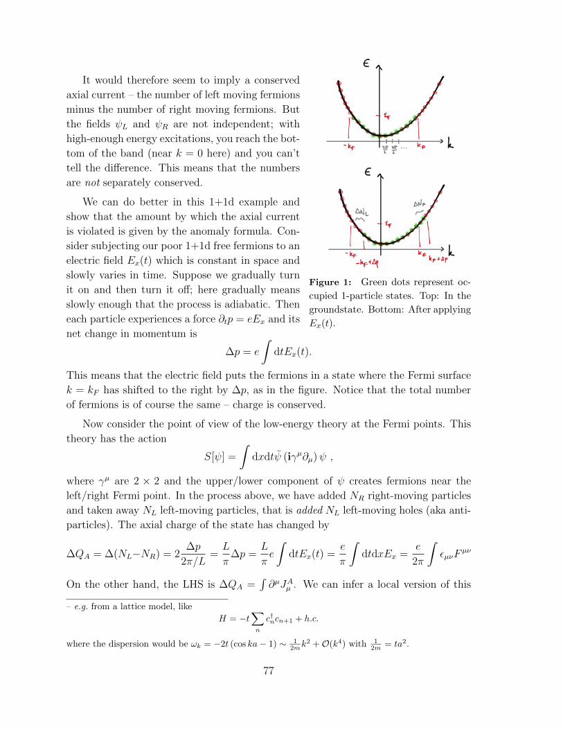
Figure 1: Green dots represent oc-
cupied 1-particle states. Top: In the
groundstate. Bottom: After applying
Ex(t).
It would therefore seem to imply a conserved
axial current – the number of left moving fermions
minus the number of right moving fermions. But
the fields ψL and ψR are not independent; with
high-enough energy excitations, you reach the bot-
tom of the band (near k = 0 here) and you can’t
tell the difference. This means that the numbers
are not separately conserved.
We can do better in this 1+1d example and
show that the amount by which the axial current
is violated is given by the anomaly formula. Con-
sider subjecting our poor 1+1d free fermions to an
electric field Ex(t) which is constant in space and
slowly varies in time. Suppose we gradually turn
it on and then turn it off; here gradually means
slowly enough that the process is adiabatic. Then
each particle experiences a force ∂tp = eEx and its
net change in momentum is
∆p = e
∫dtEx(t).
This means that the electric field puts the fermions in a state where the Fermi surface
k = kF has shifted to the right by ∆p, as in the figure. Notice that the total number
of fermions is of course the same – charge is conserved.
Now consider the point of view of the low-energy theory at the Fermi points. This
theory has the action
S[ψ] =
∫dxdtψ (iγµ∂µ)ψ ,
where γµ are 2 × 2 and the upper/lower component of ψ creates fermions near the
left/right Fermi point. In the process above, we have added NR right-moving particles
and taken away NL left-moving particles, that is added NL left-moving holes (aka anti-
particles). The axial charge of the state has changed by
∆QA = ∆(NL−NR) = 2∆p
2π/L=L
π∆p =
L
πe
∫dtEx(t) =
e
π
∫dtdxEx =
e
2π
∫εµνF
µν
On the other hand, the LHS is ∆QA =∫∂µJAµ . We can infer a local version of this
– e.g. from a lattice model, like
H = −t∑n
c†ncn+1 + h.c.
where the dispersion would be ωk = −2t (cos ka− 1) ∼ 12mk
2 +O(k4) with 12m = ta2.
77
equation by letting E vary slowly in space as well, and we conclude that
∂µJµA =
e
2πεµνF
µν .
This agrees exactly with the anomaly equation in D = 1+1 produced by the calculation
above in (12.6) (see the homework).
78
13 Saddle points, non-perturbative field theory and
resummations
13.1 Instantons in the Abelian Higgs model in D = 1 + 1
[Coleman p. 302-307] Consider the CPN−1 model in D = 1 + 1 again. What is the
force between two distant (massive) z-particles? According to (11.35), the force from
σ exchange is short-ranged: Π(q → 0) = 4πN
. But the Coulomb force, from A in
D = 1 + 1 is independent of separation (i.e. the potential∫
dp eipx
p2 ∼ x is linear). This
means confinement.
Let’s think more about abelian gauge theory in D = 1 + 1. Consider the case of
N = 1. This could be called the CP0 model, but it is usually called the Abelian Higgs
model.
L =1
4e2F 2 +Dµz
†Dµz +κ
4(z†z)2 +
µ2
2z†z + θ
F
2π.
What would a classical physicist say is the phase diagram of this model as we vary
µ2? For µ2 > 0, it is 2d scalar QED. There is no propagating photon, but (as we just
discussed) the model confines because of the Coulomb force. The spectrum is made
of boundstates of zs and z†s, which are stable because there is no photon for them
to decay into. For µ2 < 0, it looks like the potential wants |z|2 = µ2/κ ≡ v2 in the
groundstate. This would mean that Aµ eats the phase of z, gets a mass (a massive
vector in D = 1 + 1 has a propagating component); the radial excitation of z is also
massive. In such a Higgs phase, external charges don’t care about each other, the force
is short-ranged.
Not all of the statements in the classical, shaded box are correct quantumly. In
fact, even at µ2 < 0, external charges are still confined (but with a different string
tension than µ2 > 0). Non-perturbative physics makes a big difference here.
Let’s try to do the euclidean path integral at µ2 < 0 by saddle point. This means
we have to find minima of
S0E ≡
∫ (1
4e2F 2 +Dµz
†Dµz +κ
4(z†z − v2)2
)d2x.
(Ignore θ for now, since it doesn’t affect the EOM.) Where have you seen this before?
This is exactly the functional we had to minimize in §10.1 to find the (Abrikosov-
Nielsen-Olesen) vortex solution of the Abelian Higgs model. There we were thinking
about a 3+1 D field theory, and we found a static configuration, translation invariant
79
in one spatial direction, localized in the two remaining directions. Here we have only
two dimensions. The same solution of the equations now represents an instanton – a
solution of the euclidean equations of motion, localized in euclidean spacetime. Here’s
a quick review of the solution: Choosing polar coordinates about some origin (more on
this soom), the solution has (in order that V (ρ) goes to zero at large r)
z(r, θ)r→∞→ g(θ)v,
where g(θ) is a phase. We can make the |Dz|2 term happy by setting
Ar→∞→ −ig∂µg +O(r−2).
Then the F 2 term is automatically happy.
What are the possible g(θ)? g is a map from the circle at infinity to the circle
of phases g : S1 → S1. Such maps are classified by a winding number, Q ∈ Z. A
representative of each class is g(θ) = eiQθ. This function gives∫spacetime
F
2π=
∮A
2π= −i
∫ 2π
0
dθe−iQθ(+iQ)eiQθ = Q.
The winding number determines the flux.
This means the partition function is
Z =
∫[dAdz]e−S[A,z] =
∑QT∈Z
eiθQTZQT '∑QT
eiθQT e−SQT0
1
detS ′′QT.
In the last step I made a caricature of the saddle point approximation. Notice the
dependence of the instanton (Q 6= 0) contributions: if we scale out an overall coupling
(by rescaling fields) and write the action as S[φ] = 1g2S[φ, ratios of couplings], then
e−S0 = e− 1g2S[φ,ratios]
is non-analytic at g = 0 – all the terms of its taylor expansion
vanish at g = 0. This is not something we could ever produce by perturbation series, it
is non-perturbative. Notice that it is also small at weak coupling. However, sometimes
it is the leading contribution, e.g. to the energy of a metastable vacuum. (For more on
this, see Coleman.)
To do better, we need to understand the saddle points better.
1. First, in the instanton solution we found, we picked a center, the location of the
core of the vortex. But in fact, there is a solution for any center xµ0 , with the same
action. This means the determinant of S ′′ actually has a zero! The resolution is
simple: There is actually a family of saddles, labelled by the collective coordinate
xµ0 . We just have to do the integral over these coordinates. The result is simple:
80
it produces a factor of∫dDx0 = V T where V T is the volume of spacetime. The
contribution of one instanton to the integral is then
Ke−S0eiθV T
for some horrible constant K.
2. Second, since the vortex solution is localized, we can make arbitrarily-close-to-
solutions by introducing multiple vortices with their respective centers arbitrarily
far from each other. The QT is actually the sum of the instanton numbers. If they
are far enough apart, their actions also add. Each center has its own collective
coordinate and produces its own factor of V T .
3. We can also have anti-instantons. This just means that individual Qs can be
negative.
So we are going to approximate our integral by a dilute gas of instantons and anti-
instantons. Their actions add. A necessary condition for this to be a good idea is that
V T (core size)2. eiθ is the instanton fugacity.
Z = Tr e−THT→∞'
∑n,n
(Ke−S0
)n+n(V T )n+nei(n−n)θ 1
n!n!
=
(∑n
1
n!
(Ke−S0V T
)neinθ
)× (h.c.)
= eV TKe−S0eiθ+h.c. = eV T2Ke−S0 cos θ. (13.1)
We should be happy about this answer. Summing over the dilute gas of instantons
gives an extensive contribution to the free energy. The free energy per unit time in the
euclidean path integral is the groundstate energy density:
Z = Tr e−THT→∞' e−TV E(θ), =⇒ E(θ) = −2K cos θe−S0 .
[End of Lecture 53]
We can also calculate the expected flux:⟨∫F
2π
⟩=∑Q
QeiθQe−S∑Q
eiθQe−S = −i∂θ lnZ(θ) = 2KV sin θe−S0 .
Therefore, when θ 6= 0 mod π, there is a nonzero electric field in the vacuum: 〈F01〉 =
E 6= 0. It is uniform.
81
A small variation of this calculation gives the force between external charges:⟨W
2 l T ′↔L′
⟩ =⟨ei qe
∮2 Aµdx
µ⟩
=⟨ei qe
∫ F⟩
This has the effect of shifting the value of θ on the inside of the loop to θin ≡ θ+ qe2π.
So the answer in the dilute instanton gas approximation is
⟨W
2 l T ′↔L′
⟩ =
exp
2KeS0
(LT − L′T ′) cos θ︸ ︷︷ ︸inside
+L′T ′ cos θin︸ ︷︷ ︸outside
e2Ke−S0LT cos θ
= e−T′V (L′)
with
V (L′) = L′2Ke−S0
(cos θ − cos
(θ + 2π
q
e
))which is linear in the separation between the charges – linear confinement, except when
q = ne, n ∈ Z.
Here’s how to think about this result. For small θ, q/e, the potential between
charges is
V (L′)θ1' L′Ke−S0
((θ + 2π
q
e
)2
− θ2
)and the energy and flux are
E(θ)θ1' 2Ke−S0θ2 + const, 〈F 〉 θ1' 4πKe−S0θ.
θ is like the charge on a pair of parallel capacitor plates at x =∞. Adding charge and
anticharge changes the electric field in between, and the energy density is quadratic
in the field, U ∝ E2. But what happens when q = ne? Notice that the potential is
actually periodic in q → q+ne. If L′ > 12µ
(µ is the mass of the z excitations), then the
energy can be decreased by pair-creating a z and z†, which then fly to the capacitor
plates and discharge them, changing θ → θ − 2π.
Comments about D = 4. Some of the features of this story carry over to gauge
theory in D = 3 + 1. Indeed there is a close parallel between the θ∫
2F term and the
θ∫
4F ∧F term. In 4d, too, there are solutions of the euclidean equations (even in pure
Yang-Mills theory) which are localized in spacetime. (The word instanton is sometimes
used to refer to these solutions, even when they appear in other contexts than euclidean
saddle points. These solutions were found by Belavin, Polyakov, Schwartz and Tyupin.)
Again, the gauge field looks like a gauge transformation at ∞:
Ar→∞→ −ig∂µg +O(r−#).
82
Now g is a map from the 3-sphere at infinity (in euclidean 4-space) to the gauge group,
g : S3 → G. Any simple Lie group has an SU(2) ' S3 inside, and there is an integer
classification of such maps. So again there is a sum over Q ∈ Z. However: the
calculation leading to confinement does not go through so simply. The 4d θ term does
not produce a nonzero electric field in the vacuum, and an external charge isn’t like
a capacitor plate. As Coleman says, whatever causes confinement in 4d gauge theory,
it’s not instantons.
13.2 Blobology (aka Large Deviation Theory)
Many bits of the following discussion are already familiar, but I like the organization.
Feynman diagrams from the path integral. Now that we are using path
integrals all the time, the diagrammatic expansion is much less mysterious (perhaps
we should have started here, like Zee does? maybe next time). Much of what we have
to say below is still interesting for QFT in 0 + 0 dimensions, which means integrals. If
everything is positive, this is probability theory. Suppose we want to do the integral
Z(J) =
∫ ∞−∞
dq e−12m2q2− g
4!q4+Jq ≡
∫dq e−S(q) . (13.2)
It is the path integral for φ4 theory with fewer labels. For g = 0, this is a gaussian
integral which we know how to do. For g 6= 0 it’s not an elementary function of its
arguments. We can develop a (non-convergent!) series expansion in g by writing it as
Z(J) =
∫ ∞−∞
dq e−12m2q2+Jq
(1− g
4!q4 +
1
2
(− g
4!q4)2
+ · · ·)
and integrating term by term. And the term with q4n (that is, the coefficient of gn) is∫ ∞−∞
dq e−12m2q2+Jqq4n =
(∂
∂J
)4n ∫ ∞−∞
dq e−12m2q2+Jq =
(∂
∂J
)4n
e12J 1m2 J
√2π
m2.
So:
Z(J) =
√2π
m2e−
g4!(
∂∂J )
4
e12J 1m2 J .
This is a double expansion in powers of J and powers of g. The process of computing
the coefficient of Jngm can be described usefully in terms of diagrams. There is a factor
of 1/m2 for each line (the propagator), and a factor of (−g) for each 4-point vertex
(the coupling), and a factor of J for each external line (the source). For example, the
coefficient of gJ4 comes from:
∼(
1
m2
)4
gJ4.
83
There is a symmetry factor which comes from expanding the exponential: if the
diagram has some symmetry preserving the external labels, the multiplicity of diagrams
does not completely cancel the 1/n!.
As another example, consider the analog of the two-point function:
G ≡⟨q2⟩|J=0 =
∫dq q2 e−S(q)∫dq e−S(q)
= −2∂
∂m2logZ(J = 0).
In perturbation theory this is:
G '
= m−2
(1 − 1
2gm−2 +
2
3g2m−4 +O(g3)
)(13.3)
Brief comments about large orders of perturbation theory.
• How do I know the perturbation series about g = 0 doesn’t converge? One way to
see this is to notice that if I made g even infinitesimally negative, the integral itself
would not converge (the potential would be unbounded below), and Zg=−|ε| is not
defined. Therefore Zg as a function of g cannot be analytic in a neighborhood of
g = 0. This argument is due to Dyson.
• The expansion of the exponential in the integrand is clearly convergent for each
q. The place where we went wrong is exchanging the order of integration over q
and summation over n.
• The integral actually does have a name – it’s a Bessel function:
Z(J = 0) =2√m2
√ρeρK 1
4(ρ), ρ ≡ 3m4
4g
(for Re√ρ > 0), as Mathematica will tell you. Because we know about Bessel
functions, in this case we can actually figure out what happens at strong coupling,
when g m4, using the asymptotics of the Bessel function.
84
• In this case, the perturbation expansion too can be given a closed form expression:
Z(0) '√
2π
m2
∑n
(−1)n
n!
22n+ 12
(4!)nΓ
(2n+
1
2
)( g
m4
)n. (13.4)
• The expansion for G is of the form
G ' m−2
∞∑n=0
cn
( g
m4
)n.
When n is large, the coefficients satisfy cn+1n1' −2
3ncn (you can see this by
looking at the coefficients in (13.4)) so that |cn| ∼ n!. This factorial growth of
the number of diagrams is general in QFT and is another way to see that the
series does not converge.
• The fact that the coefficients cn grow means that there is a best number of orders
to keep. The errors start getting bigger when cn+1
(gm4
)∼ cn, that is, at order
n ∼ 3m4
2g. So if you want to evaluate G at this value of the coupling, you should
stop at that order of n.
• A technique called Borel resummation can sometimes produce a well-defined func-
tion of g from an asymptotic series whose coefficients diverge like n!. The idea is
to make a new series
B(z) ≡∑m=0
cmn!zm
whose coefficients are ensmallened by n!. Then to get back Z(g) we use the
identity
1 =1
n!
∫ ∞0
dze−zzn
and do the Laplace transform of B(z):∫ ∞0
dzB(z)e−z/g =∑m=0
cm
∫∞0dze−z/gzm
m!= g
∞∑m=0
cmgm = gZ(g).
This procedure requires both that the series in B(z) converges and that the
Laplace transform can be done. In fact this procedure works in this case.
The existence of saddle-point contributions to Z(g) which go like e−a/g imply
that the number of diagrams at large order grows like n!. This is because they
are associated with singularities of B(z) at z = a; such a singularity means the
sum of cnn!zn must diverge at z = a. (More generally, non-perturbative effects
which go like e−a/g1/p
(larger if p > 1) are associated with (faster) growth like
(pn)!. See this classic work.)
85
• The function G(g) can be analytically continued in g away from the real axis,
and can in fact be defined on the whole complex g plane. It has a branch cut on
the negative real axis, across which its discontinuity is related to its imaginary
part. The imaginary part goes like e−a|g| near the origin and can be computed by
a tunneling calculation.
How did we know Z has a branch cut? One way is from the asymptotics of the
Bessel function. But, better, why does Z satisfy the Bessel differential equation
as a function of the couplings? The answer, as you’ll check on the homework, is
that the Bessel equation is a Schwinger-Dyson equation,
0 =
∫ ∞−∞
∂
∂q
(somethinge−S(q)
)which results from demanding that we can change integration variables in the
path integral.
For a bit more about this, you might look at sections 3 and 4 of this recent paper from
which I got some of the details here. See also the giant book by Zinn-Justin. There is a
deep connection between the large-order behavior of the perturbation series about the
trivial saddle point and the contributions of non-trivial saddle points. The keywords
for this connection are resurgence and trans-series and a starting references is here.
The Feynman diagrams we’ve been drawing all along are the same but with more
labels. Notice that each of the qs in our integral could come with a label, q → qa. Then
each line in our diagram would be associated with a matrix (m−2)ab which is the inverse
of the quadratic term qam2abqb in the action. If our diagrams have loops we get free
sums over the label. If that label is conserved by the interactions, the vertices will have
some delta functions. In the case of translation-invariant field theories we can label
lines by the conserved momentum k. Each comes with a factor of the free propagatori
k2+m2+iε, each vertex conserves momentum, so comes with igδD (
∑k) (2π)D, and we
must integrate over momenta on internal lines∫
dDk.
Next, three general organizing facts about the diagrammatic expansion, two already
familiar. In thinking about the combinatorics below, we will represent collections of
Feynman diagrams by blobs with legs sticking out, and think about how the blobs
combine. Then we can just renormalize the appropriate blobs and be done.
The following discussion will look like I am talking about a field theory with a single
scalar field. But really each of the φs is a collection of fields and all the indices are too
small to see. This is yet another example of coarse-graining.
86
1. Disconnected diagrams exponentiate. [Zee, I.7, Banks, chapter 3] Recall
that the Feynman rules come with a (often annoying, here crucial) statement
about symmetry factors: we must divide the contribution of a given diagram
by the order of the symmetry group of the diagram (preserving various external
labels). For a diagram with k identical disconnected pieces, this symmetry group
includes the permutation group Sk which permutes the identical pieces and has
k! elements. (Recall that the origin of the symmetry factors is that symmetric
feynman diagrams fail to completely cancel the 1/n! in the Dyson formula. For
a reminder about this, see e.g. Peskin p. 93.) Therefore:
Z =∑
(all diagrams) = e∑
(connected diagrams) = eiW .
You can go a long way towards convincing yourself of this by studying the case
where there are only two connected diagrams A+B (draw whatever two squiggles
you want) and writing out eA+B in terms of disconnected diagrams with symmetry
factors.
Notice that this relationship is just like that of the partition function to the
(Helmholtz) free energy Z = e−βF (modulo the factor of i) in statistical me-
chanics (and is the same as that relationship when we study the euclidean path
integral with periodic boundary conditions in euclidean time). This statement is
extremely general. It remains true if we include external sources:
Z[J ] =
∫[Dφ]eiS[φ]+i
∫φJ = eiW [J ].
Now the diagrams have sources J at which propagator lines can terminate; (the
perturbation theory approximation to) W [J ] is the sum of all connected such
diagrams. For example
〈φ(x)〉 =1
Z
δ
iδJ(x)Z =
δ
iδJ(x)logZ =
δ
δJ(x)W
〈T φ(x)φ(y)〉 =δ
iδJ(x)
δ
iδJ(y)logZ =
δ
iδJ(x)
δ
iδJ(y)iW .
(Note that here 〈φ〉 ≡ 〈φ〉J depends on J . You can set it to zero if you want, but
the equation is true for any J .) If you forget to divide by the normalization Z,
and instead look at just δδJ(x)
δδJ(y)
Z, you get disconnected quantities like 〈φ〉 〈φ〉(the terminology comes from the diagrammatic representation). 22 The point in
life of W is that by differentiating it with respect to J we can construct all the
connected Green’s functions.22More precisely: δ
δJ(x)δ
δJ(y)Z = δδJ(x) (〈φ(x)〉J Z) = 〈φ(x)〉J 〈φ(y)〉J Z + 〈φ(x)φ(y)〉J Z.
87
2. Propagator corrections form a geometric series. This one I don’t need to
say more about:
3. The sum of all connected diagrams is the Legendre transform of the
sum of the 1PI diagrams.
[Banks, 3.8; Zee IV.3; Schwarz §34, Srednicki §21] A simpler way to say our third
fact is∑(connected diagrams) =
∑(connected tree diagrams with 1PI vertices)
where a tree diagram is one with no loops. But the description in terms of
Legendre transform will be extremely useful. Along the way we will show that
the perturbation expansion is a semi-classical expansion. And we will construct
a useful object called the 1PI effective action Γ. The basic idea is that we can
construct the actual correct correlation functions by making tree diagrams (≡diagrams with no loops) using the 1PI effective action as the action.
Notice that this is a very good reason to care about the notion of 1PI: if we
sum all the tree diagrams using the 1PI blobs, we clearly are including all the
diagrams. Now we just have to see what machinery will pick out the 1PI blobs.
The answer is: Legendre transform. There are many ways to go about showing
this, and all involve a bit of complication. Bear with me for a bit; we will learn
a lot along the way.
Def’n of φc, the ‘classical field’. Consider the functional integral for a scalar
field theory:
Z[J ] = eiW [J ] =
∫[Dφ]ei(S[φ]+
∫Jφ) . (13.5)
Define
φc(x) ≡ δW [J ]
δJ(x)=
1
Z
∫[Dφ]ei(S[φ]+
∫Jφ)φ(x) = 〈0| φ(x) |0〉 . (13.6)
This is the vacuum expectation value of the field operator, in the presence of the
source J . Note that φc(x) is a functional of J .
88
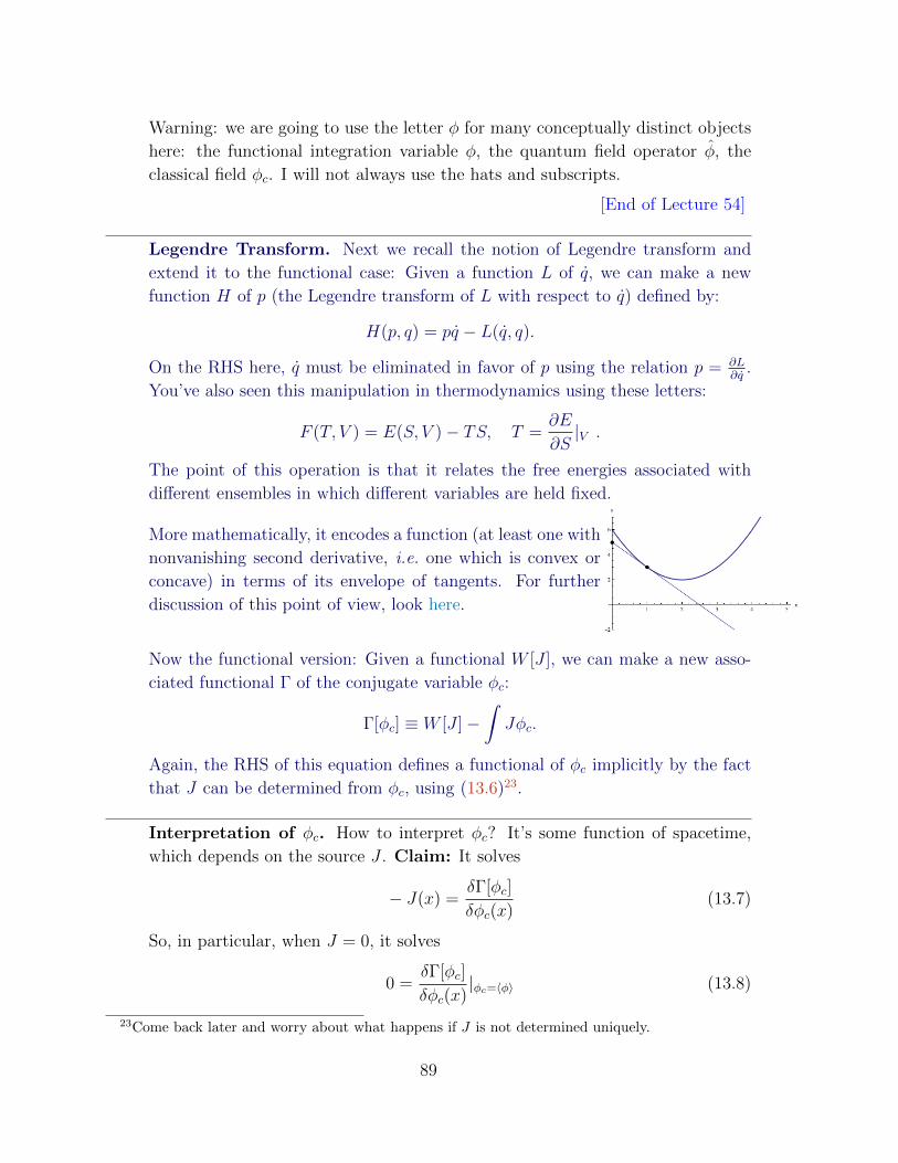
Warning: we are going to use the letter φ for many conceptually distinct objects
here: the functional integration variable φ, the quantum field operator φ, the
classical field φc. I will not always use the hats and subscripts.
[End of Lecture 54]
Legendre Transform. Next we recall the notion of Legendre transform and
extend it to the functional case: Given a function L of q, we can make a new
function H of p (the Legendre transform of L with respect to q) defined by:
H(p, q) = pq − L(q, q).
On the RHS here, q must be eliminated in favor of p using the relation p = ∂L∂q.
You’ve also seen this manipulation in thermodynamics using these letters:
F (T, V ) = E(S, V )− TS, T =∂E
∂S|V .
The point of this operation is that it relates the free energies associated with
different ensembles in which different variables are held fixed.
More mathematically, it encodes a function (at least one with
nonvanishing second derivative, i.e. one which is convex or
concave) in terms of its envelope of tangents. For further
discussion of this point of view, look here.
Now the functional version: Given a functional W [J ], we can make a new asso-
ciated functional Γ of the conjugate variable φc:
Γ[φc] ≡ W [J ]−∫Jφc.
Again, the RHS of this equation defines a functional of φc implicitly by the fact
that J can be determined from φc, using (13.6)23.
Interpretation of φc. How to interpret φc? It’s some function of spacetime,
which depends on the source J . Claim: It solves
− J(x) =δΓ[φc]
δφc(x)(13.7)
So, in particular, when J = 0, it solves
0 =δΓ[φc]
δφc(x)|φc=〈φ〉 (13.8)
23Come back later and worry about what happens if J is not determined uniquely.
89
– the extremum of the effective action is 〈φ〉. This gives a classical-like equation
of motion for the field operator expectation value in QFT.
Proof of (13.7):δΓ[φc]
δφc(x)=
δ
δφc(x)
(W [J ]−
∫dyJ(y)φc(y)
)What do we do here? We use the functional product rule – there are three places
where the derivative hits:
δΓ[φc]
δφc(x)=δW [J ]
δφc(x)− J(x)−
∫dy
δJ(y)
δφc(x)φc(y)
In the first term we must use the functional chain rule:
δW [J ]
δφc(x)=
∫dy
δJ(y)
δφc(x)
δW [J ]
δJ(y)=
∫dy
δJ(y)
δφc(x)φc(y).
So we have:
δΓ[φc]
δφc(x)=
∫dy
δJ(y)
δφc(x)φc(y)− J(x)−
∫dy
δJ(y)
δφc(x)φc(y) = −J(x). (13.9)
Now φc|J=0 = 〈φ〉. So if we set J = 0, we get the equation (13.8) above. So (13.8)
replaces the action principle in QFT – to the extent that we can calculate Γ[φc].
(Note that there can be more than one extremum of Γ. That requires further
examination.)
Next we will build towards a demonstration of the diagrammatic interpretation
of the Legendre transform; along the way we will uncover important features of
the structure of perturbation theory.
Semiclassical expansion of path integral. Recall that the Legendre trans-
form in thermodynamics is the leading term you get if you compute the partition
function by saddle point – the classical approximation. In thermodynamics, this
comes from the following manipulation: the thermal partition function is:
Z = e−βF = tre−βH =
∫dE Ω(E)︸ ︷︷ ︸
(density of states with energy E) = eS(E)
e−βEsaddle≈ eS(E?)−βE?|E? solves ∂ES=β .
The log of this equation then says F = E−TS with S eliminated in favor of T by
T = 1∂ES|V = ∂SE|V , i.e. the Legendre transform we discussed above. In simple
thermodynamics the saddle point approx is justified by the thermodynamic limit:
the quantity in the exponent is extensive, so the saddle point is well-peaked.
This part of the analogy will not always hold, and we will need to think about
fluctuations about the saddle point.
90
Let’s go back to (13.5) and think about its semiclassical expansion. If we were
going to do this path integral by stationary phase, we would solve
0 =δ
δφ(x)
(S[φ] +
∫φJ
)=
δS
δφ(x)+ J(x) . (13.10)
This determines some function φ which depends on J ; let’s denote it here as
φ[J ](x). In the semiclassical approximation to Z[J ] = eiW [J ], we would just plug
this back into the exponent of the integrand:
Wc[J ] =1
g2~
(S[φ[J ]] +
∫Jφ[J ]
).
So in this approximation, (13.10) is exactly the equation determining φc. This
is just the Legendre transformation of the original bare action S[φ] (I hope this
manipulation is also familiar from stat mech, and I promise we’re not going in
circles).
Let’s think about expanding S[φ] about such a saddle point φ[J ] (or more cor-
rectly, a point of stationary phase). The stationary phase (or semi-classical)
expansion familiar from QM is an expansion in powers of ~ (WKB):
Z = eiW/~ =
∫dx e
i~S(x) =
∫dxe
i~
S(x0)+(x−x0)S ′(x0)︸ ︷︷ ︸=0
+ 12
(x−x0)2S′′(x0)+...
= eiW0/~+iW1+i~W2+...
with W0 = S(x0), and Wn comes from (the exponentiation of) diagrams involving
n contractions of δx = x−x0, each of which comes with a power of ~: 〈δxδx〉 ∼ ~.
Expansion in ~ = expansion in coupling. Is this semiclassical expansion the
same as the expansion in powers of the coupling? Yes, if there is indeed a notion
of “the coupling”, i.e. only one for each field. Then by a rescaling of the fields
we can put all the dependence on the coupling in front:
S =1
g2s[φ]
so that the path integral is ∫[Dφ] e
is[φ]
~g2 +∫φJ.
(It may be necessary to rescale our sources J , too.) For example, suppose we are
talking about a QFT of a single field φ with action
S[φ] =
∫ ((∂φ)2
− λφp).
91
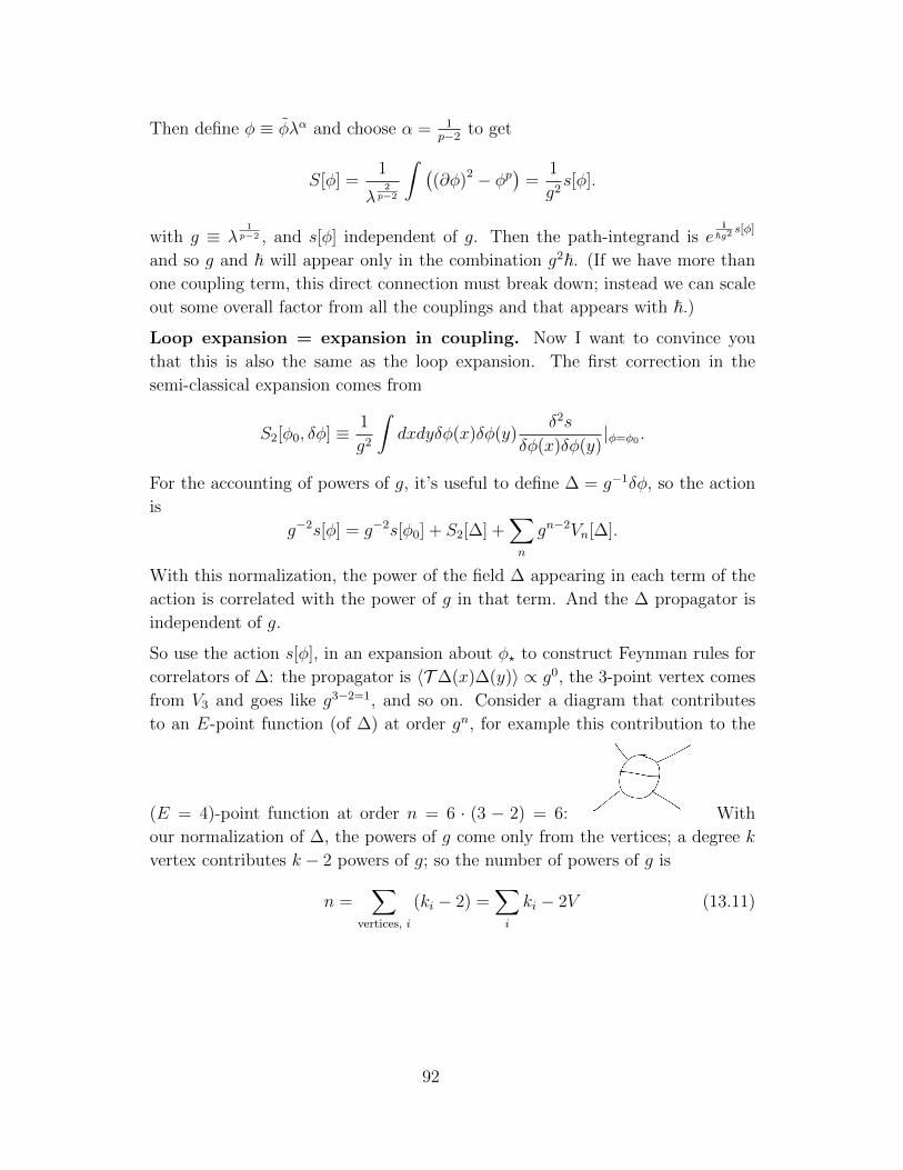
Then define φ ≡ φλα and choose α = 1p−2
to get
S[φ] =1
λ2p−2
∫ ((∂φ)2 − φp
)=
1
g2s[φ].
with g ≡ λ1p−2 , and s[φ] independent of g. Then the path-integrand is e
i~g2 s[φ]
and so g and ~ will appear only in the combination g2~. (If we have more than
one coupling term, this direct connection must break down; instead we can scale
out some overall factor from all the couplings and that appears with ~.)
Loop expansion = expansion in coupling. Now I want to convince you
that this is also the same as the loop expansion. The first correction in the
semi-classical expansion comes from
S2[φ0, δφ] ≡ 1
g2
∫dxdyδφ(x)δφ(y)
δ2s
δφ(x)δφ(y)|φ=φ0 .
For the accounting of powers of g, it’s useful to define ∆ = g−1δφ, so the action
is
g−2s[φ] = g−2s[φ0] + S2[∆] +∑n
gn−2Vn[∆].
With this normalization, the power of the field ∆ appearing in each term of the
action is correlated with the power of g in that term. And the ∆ propagator is
independent of g.
So use the action s[φ], in an expansion about φ? to construct Feynman rules for
correlators of ∆: the propagator is 〈T ∆(x)∆(y)〉 ∝ g0, the 3-point vertex comes
from V3 and goes like g3−2=1, and so on. Consider a diagram that contributes
to an E-point function (of ∆) at order gn, for example this contribution to the
(E = 4)-point function at order n = 6 · (3 − 2) = 6: With
our normalization of ∆, the powers of g come only from the vertices; a degree k
vertex contributes k − 2 powers of g; so the number of powers of g is
n =∑
vertices, i
(ki − 2) =∑i
ki − 2V (13.11)
92
where
V = # of vertices (This does not include external vertices.)
We also define:
n = # of powers of g
L = # of loops = #of independent internal momentum integrals
I = # of internal lines = # of internal propoagators
E = # of external lines
Facts about graphs:
• The total number of lines leaving all the vertices is equal to the total number
of lines: ∑vertices, i
ki = E + 2I. (13.12)
So the number of internal lines is
I =1
2
( ∑vertices, i
ki − E
). (13.13)
• For a connected graph, the number of loops is
L = I − V + 1 (13.14)
since each loop is a sequence of internal lines interrupted by vertices. (This
fact is probably best proved inductively. The generalization to graphs with
multiple disconnected components is L = I − V + C.)
We conclude that24
L(13.14)
= I − V + 1(13.13)
=1
2
(∑i
ki − E
)− V + 1 =
n− E2
+ 1(13.11)
=n− E
2+ 1.
This equation says:
L = n−E2
+ 1: More powers of g means (linearly) more loops.
24You should check that these relations are all true for some random example, like the one above,
which has I = 7, L = 2,∑ki = 18, V = 6, E = 4. You will notice that Banks has several typos in his
discussion of this in §3.4. His Es should be E/2s in the equations after (3.31).
93
Diagrams with a fixed number of external lines and more loops are suppressed
by more powers of g. (By rescaling the external field, it is possible to remove the
dependence on E.)
We can summarize what we’ve learned by writing the sum of connected graphs
as
W [J ] =∞∑L=0
(g2~)L−1
WL
where WL is the sum of connected graphs with L loops. In particular, the order-
~−1 (classical) bit W0 comes from tree graphs, graphs without loops. Solving the
classical equations of motion sums up the tree diagrams.
Diagrammatic interpretation of Legendre transform. Γ[φ] is called the 1PI
effective action25. And as its name suggests, Γ has a diagrammatic interpretation:
it is the sum of just the 1PI connected diagrams. (Recall that W [J ] is the sum
of all connected diagrams.) Consider the (functional) Taylor expansion Γn in φ
Γ[φ] =∑n
1
n!
∫Γn(x1...xn)φ(x1)...φ(xn)dDx1 · · · dDxn .
The coefficients Γn are called 1PI Green’s functions (we will justify this name
presently). To get the full connected Green’s functions, we sum all tree diagrams
with the 1PI Green’s functions as vertices, using the full connected two-point
function as the propagators.
Perhaps the simplest way to arrive at this result is to consider what happens if
we try to use Γ as the action in the path integral instead of S.
ZΓ,~[J ] ≡∫
[Dφ]ei~(Γ[φ]+
∫Jφ)
By the preceding arguments, the expansion of logZΓ[J ] in powers of ~, in the
limit ~→ 0 is
lim~→0
logZΓ,~[J ] =∑L
(g2~)L−1
W ΓL .
The leading, tree level term in the ~ expansion, is obtained by solving
δΓ
δφ(x)= −J(x)
25The 1PI effective action Γ must be distinguished from the Wilsonian effective action – the dif-
ference is that here we integrated over everybody, whereas the Wilsonian action integrates only high-
energy modes. The different effective actions correspond to different choices about what we care about
and what we don’t, and hence different choices of what modes to integrate out.
94
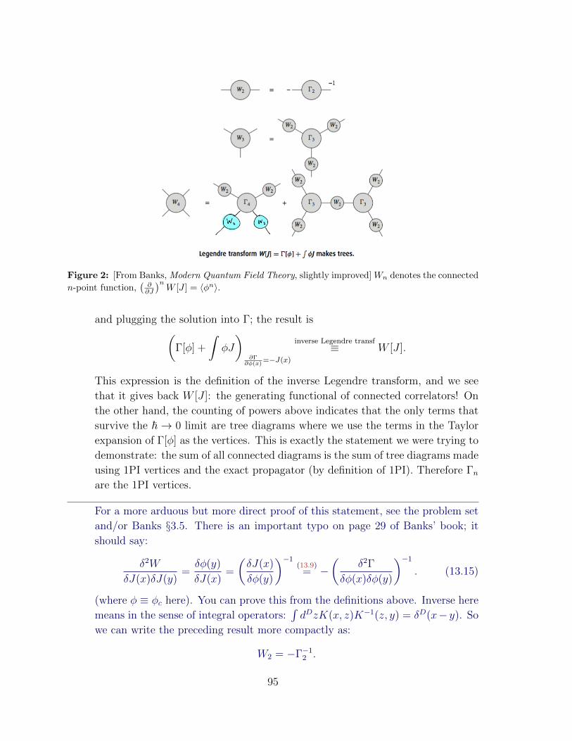
Figure 2: [From Banks, Modern Quantum Field Theory, slightly improved] Wn denotes the connected
n-point function,(∂∂J
)nW [J ] = 〈φn〉.
and plugging the solution into Γ; the result is(Γ[φ] +
∫φJ
)∂Γ
∂φ(x)=−J(x)
inverse Legendre transf≡ W [J ].
This expression is the definition of the inverse Legendre transform, and we see
that it gives back W [J ]: the generating functional of connected correlators! On
the other hand, the counting of powers above indicates that the only terms that
survive the ~ → 0 limit are tree diagrams where we use the terms in the Taylor
expansion of Γ[φ] as the vertices. This is exactly the statement we were trying to
demonstrate: the sum of all connected diagrams is the sum of tree diagrams made
using 1PI vertices and the exact propagator (by definition of 1PI). Therefore Γnare the 1PI vertices.
For a more arduous but more direct proof of this statement, see the problem set
and/or Banks §3.5. There is an important typo on page 29 of Banks’ book; it
should say:
δ2W
δJ(x)δJ(y)=δφ(y)
δJ(x)=
(δJ(x)
δφ(y)
)−1(13.9)= −
(δ2Γ
δφ(x)δφ(y)
)−1
. (13.15)
(where φ ≡ φc here). You can prove this from the definitions above. Inverse here
means in the sense of integral operators:∫dDzK(x, z)K−1(z, y) = δD(x− y). So
we can write the preceding result more compactly as:
W2 = −Γ−12 .
95
Here’s two ways to think about why we get an inverse here: (1) diagrammatically,
the 1PI blob is defined by removing the external propagators; but these external
propagators are each W2; removing two of them from one of them leaves −1 of
them. You’re on your own for the sign. (2) In the expansion of Γ =∑
n
∫Γnφ
n
in powers of the field, the second term is∫ ∫
φΓ2φ, which plays the role of the
kinetic term in the effective action (which we’re instructed to use to make tree
diagrams). The full propagator is then the inverse of the kinetic operator here,
namely Γ−12 . Again, you’re on your own for the sign.
The idea to show the general case in Fig. 2 is to just compute Wn by taking the
derivatives starting from (13.15): Differentiate again wrt J and use the matrix
differentiation formula dK−1 = −K−1dKK−1 and the chain rule to get
W3(x, y, z) =
∫dw1
∫dw2
∫dw3W2(x,w1)W2(y, w2)W2(z, w3)Γ3(w1, w2, w3) .
To get the rest of the Wn requires an induction step.
This business is useful in at least two ways. First it lets us focus our attention
on a much smaller collection of diagrams when we are doing our perturbative
renormalization.
Secondly, this notion of effective action is extremely useful in thinking about the
vacuum structure of field theories, and about spontaneous symmetry breaking.
In particular, we can expand the functional in the form
Γ[φc] =
∫dDx
(−Veff(φc) + Z(φc) (∂φc)
2 + ...)
(where the ... indicate terms with more derivatives of φ). In particular, in the
case where φc is constant in spacetime we can minimize the function Veff(φc) to
find the vacuum. This is a lucrative endeavor which you get to do for homework.
13.3 Coleman-Weinberg potential
[Zee §IV.3, Xi Yin’s notes §4.2] Let us now take seriously the lack of indices on our
field φ, and see about actually evaluating more of the semiclassical expansion of the
path integral of a scalar field (eventually we will specify D = 3 + 1):
Z[J ] = ei~W [J ] =
∫[Dφ]e
i~(S[φ]+
∫Jφ) . (13.16)
To add some drama to this discussion consider the following: if the potential V in
S =∫ (
12
(∂φ)2 − V (φ))
has a minimum at the origin, then we expect that the vacuum
96
has 〈φ〉 = 0. If on the other hand, the potential has a maximum at the origin, then
the field will find a minimum somewhere else, 〈φ〉 6= 0. If the potential has a discrete
symmetry under φ→ −φ (no odd powers of φ in V ), then in the latter case (V ′′(0) < 0)
this symmetry will be broken. If the potential is flat (V ′′(0) = 0) near the origin, what
happens? Quantum effects matter.
The configuration of stationary phase is φ = φ?, which satisfies
0 =δ(S +
∫Jφ)
δφ(x)|φ=φ? = −∂2φ?(x)− V ′(φ?(x)) + J(x) . (13.17)
Change the integration variable in (13.16) to φ = φ? +ϕ, and expand in powers of the
fluctuation ϕ:
Z[J ] = ei~(S[φ?]+
∫Jφ?)
∫[Dϕ]e
i~∫dDx 1
2((∂ϕ)2−V ′′(φ?)ϕ2+O(ϕ3))
IBP= e
i~(S[φ?]+
∫Jφ?)
∫[Dϕ]e−
i~∫dDx 1
2(ϕ(∂2+V ′′(φ?))ϕ+O(ϕ3))
≈ ei~(S[φ?]+
∫Jφ?) 1√
det (∂2 + V ′′(φ?))
= ei~(S[φ?]+
∫Jφ?)e−
12
tr log(∂2+V ′′(φ?)).
In the second line, we integrated by parts to get the ϕ integral to look like a souped-up
version of the fundamental formula of gaussian integrals – just think of ∂2 + V ′′ as a
big matrix – and in the third line, we did that integral. In the last line we used the
matrix identity tr log = log det. Note that all the φ?s appearing in this expression are
functionals of J , determined by (13.17).
So taking logs of the BHS of the previous equation we have the generating func-
tional:
W [J ] = S[φ?] +
∫Jφ? +
i~2
tr log(∂2 + V ′′(φ?)
)+O(~2) .
To find the effective potential, we need to Legendre transform to get a functional of φc:
φc(x) =δW
δJ(x)chain rule
=
∫dDz
δ(S[φ?] +
∫Jφ?
)δφ?(z)
δφ?(z)
δJ(x)+φ?(x)+O(~)
(13.17)= φ?(x)+O(~) .
The 1PI effective action is then:
Γ[φc] ≡ W −∫Jφc = S[φc] +
i~2
tr log(∂2 + V ′′(φc)
)+O(~2).
To leading order in ~, we just plug in the solution; to next order we need to compute
the sum of the logs of the eigenvalues of a differential operator. This is challenging in
97
general. In the special case that we are interested in φc which is constant in spacetime,
it is doable. This case is also often physically relevant if our goal is to solve (13.8)
to find the groundstate, which often preserves translation invariance (gradients cost
energy). If φc(x) = φ is spacetime-independent then we can write
Γ[φc(x) = φ] ≡∫dDx Veff(φ).
The computation of the trace-log is doable in this case because it is translation invari-
ant, and hence we can use fourier space. We do this next.
13.3.1 The one-loop effective potential
The tr in the one-loop contribution is a trace over the space on which the differential
operator (≡big matrix) acts; it acts on the space of scalar fields ϕ:((∂2 + V ′′(φ)
)ϕ)x
=∑y
(∂2 + V ′′(φ)
)xyϕy ≡
(∂2x + V ′′(φ)
)ϕ(x)
with matrix element (∂2 + V ′′)xy = δD(x − y) (∂2x + V ′′). (Note that in these expres-
sions, we’ve assumed φ is a background field, not the same as the fluctuation ϕ – this
operator is linear. Further we’ve assumed that that background field φ is a constant,
which greatly simplifies the problem.) The trace can be represented as a position
integral:
tr• =
∫dDx 〈x| • |x〉
so
tr log(∂2 + V ′′(φ)
)=
∫dDx 〈x| log
(∂2 + V ′′
)|x〉
=
∫dDx
∫dDk
∫dDk′ 〈x|k′〉 〈k′| log
(∂2 + V ′′
)|k〉 〈k|x〉 (1 =
∫dDk |k〉 〈k|)
=
∫dDx
∫dDk
∫dDk′ 〈x|k′〉 〈k′| log
(−k2 + V ′′
)|k〉 〈k|x〉
(〈k′| log(−k2 + V ′′
)|k〉 = δD(k − k′) log
(−k2 + V ′′
))
=
∫dDx
∫dDk log
(−k2 + V ′′
), (|| 〈x|k〉 ||2 = 1)
The∫dDx goes along for the ride and we conclude that
Veff(φ) = V (φ)− i~2
∫dDk log
(k2 − V ′′(φ)
)+O(~2).
98
What does it mean to take the log of a dimensionful thing? It means we haven’t been
careful about the additive constant (constant means independent of φ). And we don’t
need to be (unless we’re worried about dynamical gravity); so let’s choose the constant
so that
Veff(φ) = V (φ)− i~2
∫dDk log
(k2 − V ′′(φ)
k2
)+O(~2). (13.18)
[End of Lecture 55]
V1 loop =∑~k
1
2~ω~k . Here’s the interpretation of the 1-loop potential: V ′′(φ) is the
mass2 of the field when it has the constant value φ; the one-loop term V1 loop is the
vacuum energy∫dD−1~k 1
2~ω~k from the gaussian fluctuations of a field with that mass2;
it depends on the field because the mass depends on the field.
[Zee II.5.3] Why is V1 loop the vacuum energy? Recall that k2 ≡ ω2 − ~k2 and
dDk = dωdD−1~k. Consider the integrand of the spatial momentum integrals: V1 loop =
−i~2
∫dD−1~kI, with
I ≡∫
dω log
(k2 − V ′′(φ) + iε
k2 + iε
)=
∫dω log
(ω2 − ω2
k + iε
ω2 − ω2k′ + iε
)
with ωk =
√~k2 + V ′′(φ), and ωk′ = |~k|. The iε prescription is as usual inherited from
the euclidean path integral. Notice that the integral is convergent – at large ω, the
integrand goes like
log
(ω2 − Aω2 −B
)= log
(1− A
ω2
1− Bω2
)= log
(1− A−B
ω2+O
(1
ω4
))' A−B
ω2.
Integrate by parts:
I =
∫dω log
(k2 − V ′′(φ) + iε
k2 + iε
)= −
∫dωω∂ω log
(ω2 − ω2
k
ω − ωk′
)= −2
∫dωω
(ω
ω2 − ω2k + iε
− (ωk → ωk′)
)= −i2ω2
k
(1
−2ωk
)− (ωk → ωk′) = i (ωk − ωk′) .
This is what we are summing (times −i12~) over all the modes
∫dD−1~k.
99
13.3.2 Renormalization of the effective action
So we have a cute expression for the effective potential (13.18). Unfortunately it seems
to be equal to infinity. The problem, as usual, is that we assumed that the parameters in
the bare action S[φ] could be finite without introducing any cutoff. Let us parametrize
(following Zee §IV.3) the action as S =∫dDxL with
L =1
2(∂φ)2 − 1
2µ2φ2 − 1
4!λφ4 − A (∂φ)2 −Bφ2 − Cφ4
and we will think of A,B,C as counterterms, in which to absorb the cutoff dependence.
So our effective potential is actually:
Veff(φ) =1
2µ2φ2 +
1
4!λφ4 +B(Λ)φ2 + C(Λ)φ4 +
~2
∫ Λ
dDkE log
(k2E + V ′′(φ)
k2E
),
(notice that A drops out in this special case with constant φ). We rotated the integra-
tion contour to euclidean space. This permits a nice regulator, which is just to limit
the integration region to kE|k2E ≤ Λ2 for some big (Euclidean) wavenumber Λ.
Now let us specify to the case of D = 4, where the model with µ = 0 is classically
scale invariant. The integrals are elementary26
Veff(φ) =1
2µ2φ2 +
1
4!λφ4 +B(Λ)φ2 + C(Λ)φ4 +
Λ2
32π2V ′′(φ)− (V ′′(φ))2
64π2log
√eΛ2
V ′′(φ).
Notice that the leading cutoff dependence of the integral is Λ2, and there is also a
subleading logarithmically-cutoff-dependent term. (“log divergence” is certainly easier
to say.)
Luckily we have two counterterms. Consider the case where V is a quartic poly-
nomial; then V ′′ is quadratic, and (V ′′)2 is quartic. In that case the two counterterms
are in just the right form to absorb the Λ dependence. On the other hand, if V were
sextic (recall that this is in the non-renormalizable category according to our dimen-
sional analysis), we would have a fourth counterterm Dφ6, but in this case (V ′′)2 ∼ φ8,
and we’re in trouble (adding a bare φ8 term would produce (V ′′)2 ∼ φ12... and so
on). We’ll need a better way to think about such non-renormalizable theories. The
better way (which we will return to in the next section) is simply to recognize that in
non-renormalizable theories, the cutoff is real – it is part of the definition of the field
theory. In renormalizable theories, we may pretend that it is not (though it usually is
real there, too).
26This is not the same as ‘easy’. The expressions here assume that Λ V ′′.
100
Renormalization conditions. Return to the renormalizable case, V = λφ4 where
we’ve found
Veff = φ2
(1
2µ2 +B + λ
Λ2
64π2
)+ φ4
(1
4!λ+ C +
λ2
16π2log
φ2
Λ2
)+O(λ3) .
(I’ve absorbed an additive log√e in C.) The counting of counterterms works out, but
how do we determine them? We need to impose renormalization conditions, i.e. spec-
ify some observable quantities to parametrize our model, in terms of which we can
eliminate the silly letters in the lagrangian. We need two of these. Of course, what is
observable depends on the physical system at hand. Let’s suppose that we can measure
some properties of the effective potential. For example, suppose we can measure the
mass2 when φ = 0:
µ2 =∂2Veff
∂φ2|φ=0 =⇒ we should set B = −λ Λ2
64π2.
For example, we could consider the case µ = 0, when the potential is flat at the origin.
With µ = 0, have
Veff(φ) =
(1
4!λ+
λ2
(16π)2 logφ2
Λ2+ C(Λ)
)φ4 +O(λ3) .
And for the second renormalization condition, suppose we can measure the quartic
term
λM =∂4Veff
∂φ4|φ=M . (13.19)
Here M is some arbitrarily chosen quantity with dimensions of mass. We run into
trouble if we try to set it to zero because of ∂4φ (φ4 log φ) ∼ log φ. So the coupling
depends very explicitly on the value ofM at which we set the renormalization condition.
Let’s use (13.19) to eliminate C:
λ(M)!
= 4!
(λ
4!+ C +
(λ
16π
)2(log
φ2
Λ2+ c1
))|φ=M (13.20)
(where c1 is a numerical constant that you should determine) to get
Veff(φ) =1
4!λ(M)φ4 +
(λ(M)
16π
)2(log
φ2
M2− c1
)φ4 +O(λ(M)3).
Here I used the fact that we are only accurate toO(λ2) to replace λ = λ(M)+O(λ(M)2)
in various places. We can feel a sense of victory here: the dependence on the cutoff
101
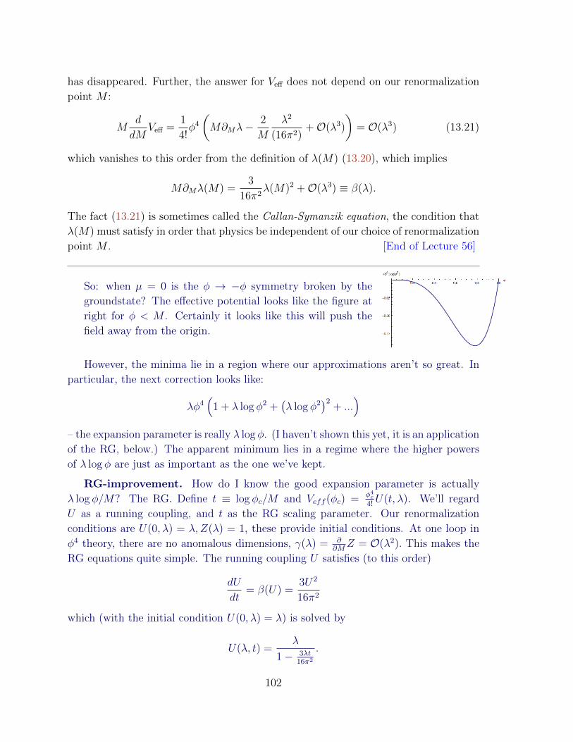
has disappeared. Further, the answer for Veff does not depend on our renormalization
point M :
Md
dMVeff =
1
4!φ4
(M∂Mλ−
2
M
λ2
(16π2)+O(λ3)
)= O(λ3) (13.21)
which vanishes to this order from the definition of λ(M) (13.20), which implies
M∂Mλ(M) =3
16π2λ(M)2 +O(λ3) ≡ β(λ).
The fact (13.21) is sometimes called the Callan-Symanzik equation, the condition that
λ(M) must satisfy in order that physics be independent of our choice of renormalization
point M . [End of Lecture 56]
So: when µ = 0 is the φ → −φ symmetry broken by the
groundstate? The effective potential looks like the figure at
right for φ < M . Certainly it looks like this will push the
field away from the origin.
However, the minima lie in a region where our approximations aren’t so great. In
particular, the next correction looks like:
λφ4(
1 + λ log φ2 +(λ log φ2
)2+ ...
)– the expansion parameter is really λ log φ. (I haven’t shown this yet, it is an application
of the RG, below.) The apparent minimum lies in a regime where the higher powers
of λ log φ are just as important as the one we’ve kept.
RG-improvement. How do I know the good expansion parameter is actually
λ log φ/M? The RG. Define t ≡ log φc/M and Veff (φc) = φ4c
4!U(t, λ). We’ll regard
U as a running coupling, and t as the RG scaling parameter. Our renormalization
conditions are U(0, λ) = λ, Z(λ) = 1, these provide initial conditions. At one loop in
φ4 theory, there are no anomalous dimensions, γ(λ) = ∂∂MZ = O(λ2). This makes the
RG equations quite simple. The running coupling U satisfies (to this order)
dU
dt= β(U) =
3U2
16π2
which (with the initial condition U(0, λ) = λ) is solved by
U(λ, t) =λ
1− 3λt16π2
.
102
Therefore, the RG-improved effective potential is
Veff (φc) =φ4c
4!U(t, λ) =
1
4!
λφ4c
1− 3λ32π2 log φ2
c
M2
.
The good news: this is valid as long as U is small, and it agrees with our previous
answer, which was valid as long as λ 1 and λt 1. The bad news is that there is
no sign of the minimum we saw in the raw one-loop answer.
By the way, in nearly every other example, there will be wavefunction renormaliza-
tion. In that case, the Callan-Syzmanzik (CS) equation we need to solve is
(−∂t + β∂λ + 4γ)U(t, λ) = 0
whose solution is
U(t, λ) = f(U(t, λ)) exp
(∫ t
0
dt′4γ(U(t′, λ))
), ∂tU(t, λ) = β(U), U(0, λ) = λ.
f can be determined by studying the CS equation at t = 0. For more detail, see
E. Weinberg’s thesis.
We can get around this issue by studying a system where the fluctuations producing
the extra terms in the potential for φ come from some other field whose mass depends
on φ. For example, consider a fermion field whose mass depends on φ:
S[ψ, φ] =
∫dDxψ (i/∂ −m− gφ)ψ
– then mψ = m + gφ. The∑
12~ωs from the fermion will now depend on φ (the also
have the opposite sign because they come from fermions), and we get a reliable answer
for 〈φ〉 6= 0 from this phenomenon of radiative symmetry breaking. In D = 1 + 1 this is
a field theory description of the Peierls instability of a 1d chain of fermions (ψ) coupled
to phonons (ψ). Notice that when φ gets an expectation value it gives a mass to the
fermions. The microscopic picture is that the translation symmetry is spontaneously
broken to a twice-as-big lattice spacing, alternating between strong and weak hopping
matrix elements. This produces a gap in the spectrum of the tight-binding model. (For
a little more, see Zee page 300.)
A second example where radiative symmetry breaking happens is scalar QED. There
we can play the gauge coupling and the scalar self-coupling off each other. I’ll say a
bit more about this example as it’s realized in condensed matter below.
Another example which has attracted a lot of attention is the Standard Model Higgs.
Its expectation value affects the masses of many fields, and you might imagine this
might produce features in its effective potential. Under various (strong) assumptions
about what lies beyond the Standard Model, there is some drama here; I recommend
Schwarz’s discussion on page 748-750.
103
13.3.3 Useful properties of the effective action
[For a version of this discussion which is better in just about every way, see Coleman,
Aspects of Symmetry §5.3.7. I also highly recommend all the preceding sections! And
the ones that come after. This book is available electronically from the UCSD library.]
Veff as minimum energy with fixed φ. Recall that 〈φ〉 is the configuration
of φc which extremizes the effective action Γ[φc]. Even away from its minimum, the
effective potential has a useful physical interpretation. It is the natural extension of
the interpretation of the potential in classical field theory, which is: V (φ) = the value
of the energy density if you fix the field equal to φ everywhere. Consider the space of
states of the QFT where the field has a given expectation value:
|Ω〉 such that 〈Ω|φ(x) |Ω〉 = φ0(x) ; (13.22)
one of them has the smallest energy. I claim that its energy is Veff(φ0). This fact, which
we’ll show next, has some useful consequences.
Let |Ωφ0〉 be the (normalized) state of the QFT which minimizes the energy subject
to the constraint (13.22). The familiar way to do this (familiar from QM, associated
with Rayleigh and Ritz)27 is to introduce Lagrange multipliers to impose (13.22) and
the normalization condition and extremize without constraints the functional
〈Ω|H |Ω〉 − α (〈Ω|Ω〉 − 1)−∫dD−1~xβ(~x) (〈Ω|φ(~x, t) |Ω〉 − φ0(~x))
with respect to |Ω〉 and the functions on space α, β. 28
27 The more familiar thing is to find the state which extremizes 〈a|H |a〉 subject to the normalization
condition 〈a|a〉 = 1. To do this, we vary 〈a|H |a〉 − E (〈a|a〉 − 1) with respect to both |a〉 and
the Lagrange multiplier E. The equation from varying |a〉 says that the extremum occurs when
(H− E) |a〉 = 0, i.e. |a〉 is an energy eigenstate with energy E. Notice that we could just as well have
varied the simpler thing
〈a| (H− E) |a〉
and found the same answer.28 Here is the QM version (i.e. the same thing without all the labels): we want to find the extremum
of 〈a|H|a〉 with |a〉 normalized and 〈a|A|a〉 = Ac some fixed number. Then we introduce two Lagrange
multipliers E, J and vary without constraint the quantity
〈a| (H− E − JA) |a〉
(plus irrelevant constants). The solution satisfies
(H− E − JA) |a〉 = 0
so |a〉 is an eigenstate of the perturbed hamiltonian H− JA, with energy E. J is an auxiliary thing,
104

Clearly the extremum with respect to α, β imposes the desired constraints. Ex-
tremizing with respect to |Ω〉 gives:
H |Ω〉 = α |Ω〉+
∫dD−1~xβ(~x)φ(~x, t) |Ω〉 (13.23)
or (H−
∫dD−1~xβ(~x)φ(~x, t)
)|Ω〉 = α |Ω〉 (13.24)
Note that α, β are functionals of φ0. We can interpret the operator Hβ ≡ H −∫dD−1~xβ(~x)φ(~x, t) on the LHS of (13.24) as the hamiltonian with a source β; and
α is the groundstate energy in the presence of that source. (Note that that source is
chosen so that 〈φ〉 = φ0 – it is a functional of φ0.)
This groundstate energy is related to the generating functional W [J = β] as we’ve
seen several times – eiW [β] is the vacuum persistence amplitude in the presence of the
source
eiW [β] =⟨
0|T ei∫βφ|0
⟩= 〈0β| e−iTHβ |0β〉 = e−iαT (13.25)
where T is the time duration. (If you want, you could imagine that we are adiabatically
turning on the interactions for a time duration T .)
The actual extremal energy (of the unperturbed hamiltonian, with constrained
expectation value of φ) is obtained by taking the overlap of (13.23) with 〈Ω| (really all
the Ωs below are Ωφ0s):
〈Ω|H |Ω〉 = α 〈Ω|Ω〉+
∫dD−1~xβ(~x) 〈Ω|φ(~x, t)|Ω〉
= α +
∫dD−1~xβ(~x)φ0(~x)
(13.25)=
1
T
(−W [β] +
∫dDxβ(~x)φ0(~x)
)Legendre
= − 1
TΓ[φ0]
φ = φ0, const=
∫dD−1~xVeff(φ0).
Cluster decomposition. The relationship (13.25) between the generating func-
tional W [J ] (for time-independent J) and the energy in the presence of the source is
which really depends on our choice Ac, via
Ac = 〈a|A|a〉 = −dEdJ
.
(If you like, we used the Feynman-Hellmann theorem, dEdJ =⟨dHdJ
⟩.) The quantity we extremized is
〈a|H|a〉 = E + JAc = E − J dEdJ
.
This Legendre transform is exactly (the QM analog of) the effective potential.
105
very useful. (You’ve previously used it on the homework to compute the potential
between static sources, and to calculate the probability for pair creation in an electric
field.) Notice that it gives an independent proof that W only gets contributions from
connected amplitudes. Amplitudes with n connected components, 〈....〉 〈...〉 〈...〉︸ ︷︷ ︸n of these
, go
like T n (where T is the time duration) at large T . Since W = −EJT goes like T 1,
we conclude that it has one connected component (terms that went like T n>1 would
dominate at large T and therefore must be absent). This extensivity of W in T is of
the same nature as the extensivity in volume of the free energy in thermodynamics.
[Brown, 6.4.2] Another important reason why W must be connected is called
the cluster decomposition property. Consider a source which has the form J(x) =
J1(x) + J2(x) where the two parts have support in widely-separated (spacelike sepa-
rated) spacetime regions. If all the fields are massive, ‘widely-separated’ means pre-
cisely that the distance between the regions is R 1/m, much larger than the range
of the interactions mediated by φ. In this case, measurements made in region 1 can-
not have any effect on those in region 2, and they should be uncorrelated. If so, the
probability amplitude factorizes
Z[J1 + J2] = Z[J1]Z[J2]
which by the magic of logs is the same as
W [J1 + J2] = W [J1] +W [J2].
If W were not connected, it would not have this additive property.
There are actually some exceptions to cluster decomposition arising from situations
where we prepare an initial state (it could be the groundstate for some hamiltonian) in
which there are correlations between the excitations in the widely separated regions.
Such a thing happens in situations with spontaneous symmetry breaking, where the
value of the field is the same everywhere in space, and therefore correlates distant
regions.
Convexity of the effective potential. Another important property of the ef-
fective potential is V ′′eff(φ) > 0 – the effective potential is convex (sometimes called
‘concave up’). We can see this directly from our previous work. Most simply, recall
that the functional Taylor coefficients of Γ[φ] are the 1PI Green’s functions; Veff is just
Γ evaluated for constant φ, i.e. zero momentum; therefore the Taylor coefficients of Veff
are the 1PI Green’s functions at zero momentum. In particular, V ′′eff(φ) = 〈φk=0φk=0〉:the ground state expectation value of the square of a hermitian operator, which is
106
positive.29 30
On the other hand, it seems that if V (φ) has a maximum, or even any region of
field space where V ′′(φ) < 0, we get a complex one-loop effective potential (from the
log of a negative V ′′). What gives? One resolution is that in this case the minimum
energy state with fixed 〈φ〉 is not a φ eigenstate.
For example, consider a quartic potential 12m2φ2 + g
4!φ4 with m2 < 0, with minima
at φ± ≡ ±√
6|m|2g
. Then for 〈φ〉 ∈ (φ−, φ+), rather we can lower the energy below V (φ)
by considering a state
|Ω〉 = c+ |Ω+〉+ c− |Ω−〉 , 〈Ω|φ|Ω〉 = |c+|2φ+ + |c−|2φ−.
The one-loop effective potential at φ only knows about some infinitesimal neighborhood
of the field space near φ, and fails to see this non-perturbative stuff. In fact, the correct
effective potential is exactly flat in between the two minima. More generally, if the two
minima have unequal energies, we have
Veff = 〈Ω|H |Ω〉 = |c+|2V (φ+) + |c−|2V (φ−)
– the potential interpolates linearly between the energies of the two surrounding min-
ima.
The imaginary part of V1 loop is a decay rate. If we find that the (pertur-
bative approximation to) effective potential E ≡ V1 loop is complex, it means that the
amplitude for our state to persist is not just a phase:
A ≡ 〈0| e−iTH |0〉 = e−iEVT
29More explicitly: Begin from Veff = − ΓV .
∂
∂φ0Veff(φ0) = −
∫dDx
Vδ
δφ(x)
Γ[φ]
V|φ(x)=φ0
(13.7)= − 1
V
∫dDx
V(−J(x)) |φ(x)=φ0
.
In the first expression here, we are averaging over space the functional derivative of Γ. The second
derivative is then(∂
∂φ0
)2
Veff(φ0) =1
V
∫dDy
Vδ
δφ(y)
∫dDx
V(J(x)) |φ(x)=φ0
= +1
V3
∫y
∫x
δJ(x)
δφ(y)|φ(x)=φ0
Using (13.15), this is
V ′′eff = +1
V3
∫y
∫x
(W−1
2
)xy
– the inverse is in a matrix sense, with x, y as matrix indices. But W2 is a positive operator – it is
the groundstate expectation value of the square of a hermitian operator.30In fact, the whole effective action Γ[φ] is a convex functional: δ2Γ
δφ(x)δφ(y) is a positive integral
operator. For more on this, I recommend Brown, Quantum Field Theory, Chapter 6.
107
has a modulus different from one (V is the volume of space). Notice that the |0〉 here
is our perturbative approximation to the groundstate of the system, which is wrong in
the region of field space where V ′′ < 0. The modulus of this object is
Pno decay = ||A ||2 = e−VT2ImE
– we can interpret 2ImE as the (connected!) decay probability of the state in question
per unit time per unit volume. (Notice that this relation means that the imaginary
part of V1-loop had better be positive, so that the probability stays less than one! In the
one-loop approximation, this is guaranteed by the correct iε prescription.)
For more on what happens when the perturbative answer becomes complex and
non-convex, and how to interpret the imaginary part, see this paper by E. Weinberg
and Wu.
108
14 Duality
14.1 XY transition from superfluid to Mott insulator, and T-
duality
In this subsection and the next we’re going to think about ways to think about bosonic
field theories with a U(1) symmetry, and dualities between them, in D = 1 + 1 and
D = 2 + 1.
[This discussion is from Ashvin Vishwanath’s lecture notes.] Consider the Bose-
Hubbard model (in any dimension, but we’ll specify to D = 1 + 1 at some point)
HBH = −J∑〈ij〉
(b†ibj + h.c.
)+U
2
∑i
ni (ni − 1)− µ∑i
ni
where the b†s and b are bosonic creation and annihilation operators at each site:
[bi,b†j] = δij. ni ≡ b†ibi counts the number of bosons at site i. The last Hubbard-U
term is zero if nbj = 0, 1, but exacts an energetic penalty ∆E = U if a single site j is
occupied by two bosons.
The Hilbert space which represents the boson algebra has a useful number-phase
representation in terms of
[ni, φj] = −iδij, φi ≡ φi + 2π, ni ∈ Z
(where the last statement pertains to the eigenvalues of the operator). The bosons are
bi = e−iφi√
ni, b†i =√
nie+iφi ;
these expressions have the same algebra as the original bs. In terms of these operators,
the hamiltonian is
HBH = −J∑〈ij〉
(√nie
i(φi−φj)√nj + h.c.)
+U
2
∑i
ni (ni − 1)− µ∑i
ni.
If 〈ni〉 = n0 1, so that ni = n0 + ∆ni,∆ni n0 then bi = e−iφ√ni ' e−iφi√n0
and
HBH ' − 2Jn0︸ ︷︷ ︸≡J
∑〈ij〉
cos (φi − φj) +U
2
∑i
(∆ni)2 ≡ Hrotors
where we set n0 ≡ µ/U 1. This is a rotor model.
This model has two phases:
U J : then we must satisfy the U term first and the number is locked, ∆n = 0 in
109
the groundstate. This is a Mott insulator, with a gap of order U . Since n and φ are
conjugate variables, definite number means wildly fluctuating phase.
U J : then we must satisfy the J term first and the phase is locked, φ = 0 in
the groundstate, or at least it will try. This is the superfluid (SF). That is, we can try
to expand the cosine potential31
Hrotors = U∑i
n2i − J
∑〈ij〉
cos (φi − φj) ' U∑i
n2i − J
∑〈ij〉
(1− 1
2(φi − φj)2 + ...
)(14.1)
which is a bunch of harmonic oscillators and can be solved by Fourier: φi = 1√Nd
∑i e−ik·xiφk,
so
H '∑k
(Uπkπ−k + J (1− cos ka)φkφ−k)
This has gapless phonon modes at k = 0, whose existence is predicted by Nambu-
Goldstone. I have written the hamiltonian in 1d notation but nothing has required it
so far. The low energy physics is described by the continuum lagrangian density
Leff =ρs2
((∂τφ)2
c+ c(~∇φ)2)
(14.2)
with ρs =√J/U, c =
√JU . ρs is called the superfluid stiffness. This is a free massless
scalar theory. The demand of the U(1) symmetry φ→ φ+α forbids interactions which
would be relevant; the only allowed interactions are derivative interactions (as you can
see by keeping more terms in the Taylor expansion (14.1)) such as (∂φ)4.
Now 1d comes in: In d > 1, there is long range order – the bosons condense and
spontaneously break the phase rotation symmetry φ → φ + α; the variable φ is a
Goldstone boson. In 1d there is no long-range order. The two phases are still distinct
however, since one has a gap and the other does not. The correlators of the boson
operator bi ∼ eiφi diagnose the difference. In the Mott phase they have exponential
decay. In the “SF” they have⟨eiφ(x)e−iφ(y)
⟩=c0
rη, η =
1
2πρs=
1
2K.
This is algebraic long range order. This is a sharp distinction between the two phases
we’ve discussed, even though the IR fluctuations destroy the 〈b〉.
[End of Lecture 57]
31From now on the background density n0 will not play a role and I will write ni for ∆ni.
110
Massless scalars in D = 1 + 1 and T -duality-invariance of the spectrum.
A lot of physics is hidden in the innocent-looking theory of the superfluid goldstone
boson. Consider the following (real-time) continuum action for a free massless scalar
field in 1+1 dimensions:
S[φ] =T
2
∫dt
∫ L
0
dx((∂0φ)2 − (∂xφ)2) = 2T
∫dxdt∂+φ∂−φ . (14.3)
I have set the velocity of the bosons to c = 1 by rescaling t. Here x± ≡ t ± x are
lightcone coordinates; the derivatives are ∂± ≡ 12
(∂t ± ∂x). Space is a circle: the point
labelled x is the same as the point labelled x+ L.
We will assume that the field space of φ itself is periodic:
φ(x, t) ≡ φ(x, t) + 2π, ∀x, t .
So the field space is a circle S1 with (angular) coordinate φ. It can be useful to think
of the action (14.3) as describing the propagation of a string, since a field configuration
describes an embedding of the real two dimensional space into the target space, which
here is a circle. This is a simple special case of a nonlinear sigma model. The name
T-duality comes from the literature on string theory. The worldsheet theory of a string
propagating on a circle of radius R =√ρs is governed by the Lagrangian (14.2). To
see this, recall that the action of a 2d nonlinear sigma model with target space metric
gµνφµφν is 1
α′
∫d2σgµν∂φ
µ∂φν . Here 1α′
is the tension (energy per unit length) of the
string; work in units where this disappears from now on. Here we have only one
dimension, with gφφ = ρs.
Notice that we could rescale φ→ λφ and change the radius; but this would change
the periodicity of φ ≡ φ+ 2π. The proper length of the period is 2πR and is invariant
under a change of field variables. This proper length distinguishes different theories
because the operators : eαφ : (which you saw on a previous homework were good
operators of definite scaling dimension in the theory of the free boson (unlike φ itself))
must be periodic; this determines the allowed values of α.
First a little bit of classical field theory. The equations of motion for φ are
0 =δS
δφ(x, t)∝ ∂µ∂µφ ∝ ∂+∂−φ
which is solved by
φ(x, t) ≡ φL(x+) + φR(x−) .
In euclidean time, φL,R depend (anti-)holomorphically on the complex coordinate z ≡12(x+ iτ) and the machinery of complex analysis becomes useful.
111
Symmetries: Since S[φ] only depends on φ through its derivatives, there is a
simple symmetry φ→ φ+ ε. By the Nother method the associated current is
jµ = T∂µφ . (14.4)
This symmetry is translations in the target space, and I will sometimes call the asso-
ciated conserved charge ‘momentum’.
There is another symmetry which is less obvious. It comes about because of the
topology of the target space. Since φ(x, t) ≡ φ(x, t) + 2πm,m ∈ Z describe the same
point (it is a redundancy in our description, in fact a discrete gauge redundancy), we
don’t need φ(x+ L, t) = φ(x, t). It is enough to have
φ(x+ L, t) = φ(x, t) + 2πm, m ∈ Z
The number m cannot change without the string breaking: it is a topological charge,
a winding number:
m =1
2πφ(x, t)|x=L
x=0FTC=
1
2π
∫ L
0
dx∂xφ . (14.5)
The associated current whose charge density is 1π∂xφ (which integrates over space to
the topological charge) is
jµ =1
2π(∂xφ,−∂0φ)µ =
1
2πεµν∂νφ.
This is conserved because of the equality of the mixed partials: εµν∂µ∂ν = 0.
Let’s expand in normal modes: φ = φL + φR with
φL(t+ x) = qL + (p+ w)︸ ︷︷ ︸≡ 1
2TpL
(t+ x)− i
√L
4πT
∑n6=0
ρnnein(t+x) 2π
L ,
φR(t− x) = qR + (p− w)︸ ︷︷ ︸≡ 1
2TpR
(t− x)− i
√L
4πT
∑n6=0
ρnnein(t−x) 2π
L , (14.6)
The factor of 1n
is a convention whose origin you will appreciate below, as are the other
normalization factors. Real φ means ρ†n = ρ−n (If we didn’t put the i it would have
been −ρ−n).
Here q ≡ 1L
∫ L0dxφ(x, t) = qL − qR is the center-of-mass position of the string. The
canonical momentum for φ is π(x, t) = T∂0φ(x, t) = T (∂+φL + ∂−φR).
QM. Now we’ll do quantum mechanics. Recall that a quantum mechanical particle
on a circle has momentum quantized in units of integers over the period. Since φ is
112
periodic, the wavefunction(al)s must be periodic in the center-of-mass coordinate q
with period 2π, and this means that the total (target-space) momentum must be an
integer
Z 3 j = π0 ≡∫ L
0
dxπ(x, t) = T
∫ L
0
dx∂tφ(14.6)= LT2p
So our conserved charges are quantized according to
p =j
2LT, w
(14.6)(14.5)=
πm
L, j,m ∈ Z .
(Don’t confuse the target-space momentum j with the ‘worldsheet momentum’ n!)
(Note that this theory is scale-free. We could use this freedom to choose units where
L = 2π.)
Now I put the mode coefficients in boldface:
φL(x+) = qL +1
2TpLx
+ − i
√L
4πT
∑n 6=0
ρnnei 2π
Lnx+
,
φR(x−) = qR +1
2TpRx
− − i
√L
4πT
∑n6=0
ρnnei 2π
Lnx− , (14.7)
The nonzero canonical equal-time commutators are
[φ(x),π(x′)] = −iδ(x− x′)
which determines the commutators of the modes (this was the motivation for the weird
normalizations)
[qL,pL] = [qR,pR] = i, [ρn,ρ†n′ ] = nδn,n′ , or [ρn,ρn′ ] = nδn+n′ ,
and the same for the rightmovers with twiddles. This is one simple harmonic oscillator
for each n ≥ 1 (and each chirality); the funny normalization is conventional.
H =
∫dx(π(x)φ(x)− L
)=
1
2
∫dx
(π2
T+ T (∂xφ)2
)= L
1
4T
(p2L + p2
R
)︸ ︷︷ ︸π2
02T
+T2
w2
+π∞∑n=1
(ρ−nρn + ρ−nρn) + a
=1
2L
(j2
T+ T (2πm)2
)+ π
∞∑n=1
n(Nn + Nn
)+ a (14.8)
Here a is a (UV sensitive) constant which will not be important for us (it is very
important in string theory), which is the price we pay for writing the hamiltonian as
113
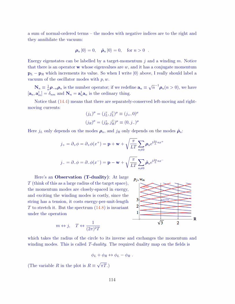
a sum of normal-ordered terms – the modes with negative indices are to the right and
they annihilate the vacuum:
ρn |0〉 = 0, ρn |0〉 = 0, for n > 0 .
Energy eigenstates can be labelled by a target-momentum j and a winding m. Notice
that there is an operator w whose eigenvalues are w, and it has a conjugate momentum
pL − pR which increments its value. So when I write |0〉 above, I really should label a
vacuum of the oscillator modes with p, w.
Nn ≡ 1nρ−nρn is the number operator; if we redefine an ≡
√n−1ρn(n > 0), we have
[an, a†m] = δnm and Nn = a†nan is the ordinary thing.
Notice that (14.4) means that there are separately-conserved left-moving and right-
moving currents:
(jL)µ = (jzL, jzL)µ ≡ (j+, 0)µ
(jR)µ = (jzR, jzR)µ ≡ (0, j−)µ
Here jL only depends on the modes ρn, and jR only depends on the modes ρn:
j+ = ∂+φ = ∂+φ(x+) = p + w +
√π
LT
∑n6=0
ρnei 2πLnx+
j− = ∂−φ = ∂−φ(x−) = p−w +
√π
LT
∑n6=0
ρnei 2πLnx−
Here’s an Observation (T-duality): At large
T (think of this as a large radius of the target space),
the momentum modes are closely-spaced in energy,
and exciting the winding modes is costly, since the
string has a tension, it costs energy-per-unit-length
T to stretch it. But the spectrum (14.8) is invariant
under the operation
m↔ j, T ↔ 1
(2π)2T
which takes the radius of the circle to its inverse and exchanges the momentum and
winding modes. This is called T-duality. The required duality map on the fields is
φL + φR ↔ φL − φR .
(The variable R in the plot is R ≡√πT .)
114
T-duality says string theory on a large circle is the same as string theory on a
small circle. On the homework you’ll get to see a derivation of this statement in the
continuum which allows some generalizations.
Vertex operators. It is worthwhile to pause for another moment and think about
the operators which create the winding modes. They are like vortex creation operators.
Since φ has logarithmic correlators, you might think that exponentiating it is a good
idea. First let’s take advantage of the fact that the φ correlations split into left and
right bits to write φ(z, z) = φL(z) + φR(z):
〈φL(z)φL(0)〉 = − 1
πTlog
z
a, 〈φR(z)φR(0)〉 = − 1
πTlog
z
a, 〈φL(z)φR(0)〉 = 0 .
(14.9)
A set of operators with definite scaling dimension is:
Vα,β(z, z) =: ei(αφL(z)+βφR(z)) : .
This is a composite operator which we have defined by normal-ordering. The normal
ordering prescription is: q, p,−,+ , that is: positive-momentum modes (lowering op-
erators) go on the right, and p counts as a lowering operator, so in particular using the
expansion (please beware my factors here): φL(z) = qL + pLz + i∑
n6=0ρnnwn, we have
: eiαφL(z) :≡ eiαqLeiαpLzeiα∑n<0
ρnnwneiα
∑n>0
ρnnwn
(I used the definition w ≡ e2πiz/L.)
How should we think about this operator ? In the QM of a free particle, the operator
eipx inserts momentum p – it takes a momentum-space wavefunction ψ(p0) = 〈p0|ψ〉and gives
〈p0| eipx |ψ〉 = ψ(p0 + p).
It’s the same thing here, with one more twist.
In order for Vα,β to be well-defined under φ→ φ+2π, we’d better have α+β ∈ Z –
momentum is quantized, just like for the particle (the center of mass is just a particle).
Let’s consider what the operator Vα,β does to a winding and momentum eigenstate
|w, p〉 (with no oscillator excitations, ρn |p, w〉 = 0, n < 0):
Vαβ(0) |w, p〉 = ei(α+β)q0ei(α−β)φ0eiα∑n<0 ρneiα
∑n>0 ρn |w, p〉 = eiα
∑n<0 ρn |w + α− β, p+ α + β〉
(14.10)
The monster in front here creates oscillator excitations. I wrote q0 ≡ qL + qR and
φ0 ≡ qL−qR. The important thing is that the winding number has been incremented
by α− β; this means that α− β must be an integer, too. We conclude that
α + β ∈ Z, α− β ∈ Z (14.11)
115
so they can both be half-integer, or they can both be integers.
By doing the gaussian integral (or moving the annihilation operators to the right)
their correlators are
〈Vα,β(z, z)Vα′,β′(0, 0)〉 =D0
zα2
πT zβ2
πT
. (14.12)
The zeromode prefactor D0 is:
D0 =⟨ei((α+α′)qL+(β+β′)qR)
⟩0
= δα+α′δβ+β′ .
This is charge conservation.
We conclude that the operator Vα,β has scaling dimension
(hL, hR) =1
2πT(α2, β2).
Notice the remarkable fact that the exponential of a dimension-zero operator manages
to have nonzero scaling dimension. This requires that the multiplicative prefactor
depend on the cutoff a to the appropriate power (and it is therefore nonuniversal). We
could perform a multiplicative renormalization of our operators V to remove this cutoff
dependence from the correlators.
The values of α, β allowed by single-valuedness of φ and its wavefunctional are
integers. We see (at least) three special values of the parameter T :
• The SU(2) radius: When 2πT = 1, the operators with (n,m) = 1 are marginal.
Also, the operators with (n,m) = (1, 0) and (n,m) = (0, 1) have the scaling
behavior of currents, and by holomorphicity are in fact conserved.
• The free fermion radius: when 2πT = 2, V1,0 has dimension (12, 0), which is
the dimension of a left-moving free fermion, with action∫dtdxψ∂+ψ. In fact the
scalar theory with this radius is equivalent to a massless Dirac fermion! This
equivalence is an example of bosonization. In particular, the radius-changing de-
formation of the boson maps to a marginal four-fermion interaction: by studying
free bosons we can learn about interacting fermions. Should I say more about
this?
• The supersymmetric radius: when 2πT = 23, V1,0 has dimension (3
2, 0) and
represents a supersymmetry current.
After this detour, let’s turn to the drama of the bose-Hubbard model. Starting
from large J/U , where we found a superfluid, what happens as U grows and makes
116
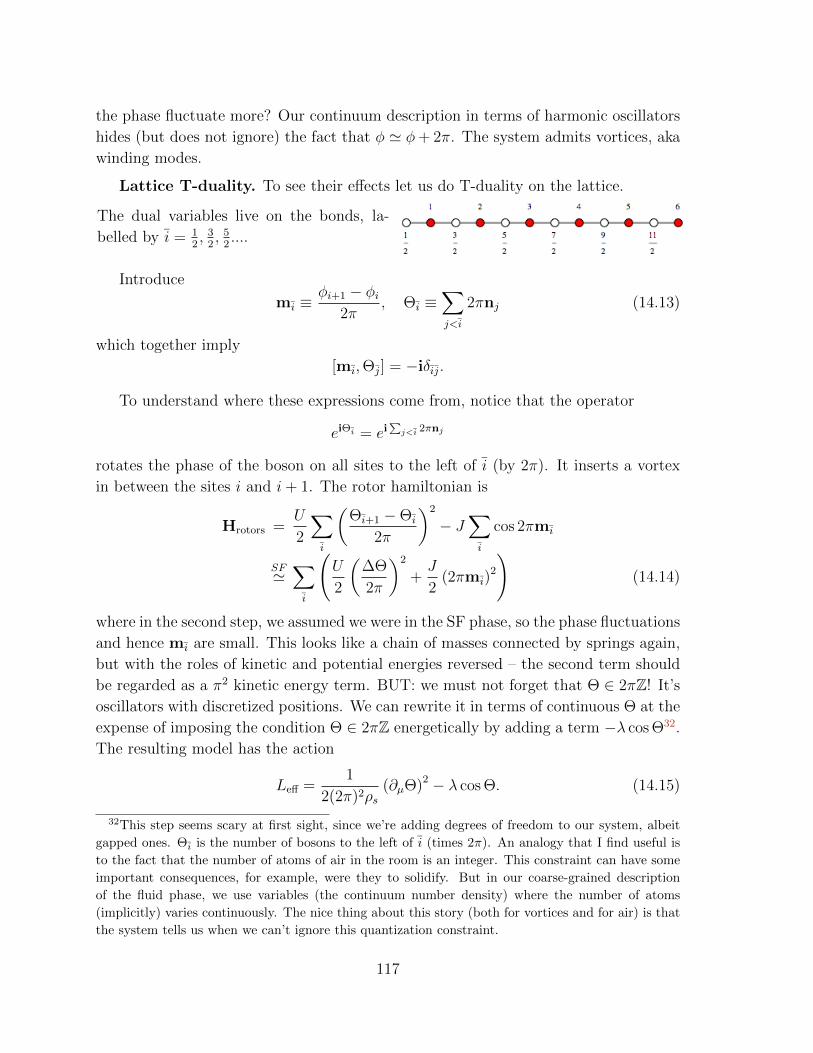
the phase fluctuate more? Our continuum description in terms of harmonic oscillators
hides (but does not ignore) the fact that φ ' φ+ 2π. The system admits vortices, aka
winding modes.
Lattice T-duality. To see their effects let us do T-duality on the lattice.
The dual variables live on the bonds, la-
belled by i = 12, 3
2, 5
2....
Introduce
mi ≡φi+1 − φi
2π, Θi ≡
∑j<i
2πnj (14.13)
which together imply
[mi,Θj] = −iδij.
To understand where these expressions come from, notice that the operator
eiΘi = ei∑j<i 2πnj
rotates the phase of the boson on all sites to the left of i (by 2π). It inserts a vortex
in between the sites i and i+ 1. The rotor hamiltonian is
Hrotors =U
2
∑i
(Θi+1 −Θi
2π
)2
− J∑i
cos 2πmi
SF'∑i
(U
2
(∆Θ
2π
)2
+J
2(2πmi)
2
)(14.14)
where in the second step, we assumed we were in the SF phase, so the phase fluctuations
and hence mi are small. This looks like a chain of masses connected by springs again,
but with the roles of kinetic and potential energies reversed – the second term should
be regarded as a π2 kinetic energy term. BUT: we must not forget that Θ ∈ 2πZ! It’s
oscillators with discretized positions. We can rewrite it in terms of continuous Θ at the
expense of imposing the condition Θ ∈ 2πZ energetically by adding a term −λ cos Θ32.
The resulting model has the action
Leff =1
2(2π)2ρs(∂µΘ)2 − λ cos Θ. (14.15)
32This step seems scary at first sight, since we’re adding degrees of freedom to our system, albeit
gapped ones. Θi is the number of bosons to the left of i (times 2π). An analogy that I find useful is
to the fact that the number of atoms of air in the room is an integer. This constraint can have some
important consequences, for example, were they to solidify. But in our coarse-grained description
of the fluid phase, we use variables (the continuum number density) where the number of atoms
(implicitly) varies continuously. The nice thing about this story (both for vortices and for air) is that
the system tells us when we can’t ignore this quantization constraint.
117
Ignoring the λ term, this is the T-dual action, with ρs replaced by 1(2π)2ρs
. The coupling
got inverted here because in the dual variables it’s the J term that’s like the π2 inertia
term, and the U term is like the restoring force. This Θ = φL− φR is therefore T-dual
variable, with ETCRs
[φ(x),Θ(y)] = 2πisign(x− y). (14.16)
This commutator follows directly from the definition of Θ (14.13). (14.16) means that
the operator cos Θ(x) jumps the SF phase variable φ by 2π – it inserts a 2π vortex, as
we designed it to do. So λ is like a chemical potential for vortices.
This system has two regimes, depending on the scaling dimension of the vortex
insertion operator:
• If λ is an irrelevant coupling, we can ignore it in the IR and we get a superfluid,
with algebraic LRO.
• If the vortices are relevant, λ → ∞ in the IR, and we pin the dual phase, Θi =
0,∀i. This is the Mott insulator, since Θi = 0 means ni = 0 – the number fluctuations
are frozen.
When is λ relevant? Expanding around the free theory,⟨eiΘ(x)e−iΘ(0)
⟩=
c
x2πρs
this has scaling dimension ∆ = πρs which is relevant if 2 > ∆ = πρs. Since the bose
correlators behave as⟨b†b⟩∼ x−η with η = 1
2πρs, we see that only if η < 1
4do we
have a stable SF phase. (Recall that ρs =√J/U .) If η > 1
4, the SF is unstable to
proliferation of vortices and we end up in the Mott insulator, where the quantization of
particle number matters. A lesson: we can think of the Mott insulator as a condensate
of vortices. [End of Lecture 58]
Note: If we think about this euclidean field theory as a 2+0 dimensional stat-mech
problem, the role of the varying ρs is played by temperature, and this transition we’ve
found of the XY model, where by varying the radius the vortices become relevant, is
the Kosterlitz-Thouless transition. Most continuous phase transitions occur by tuning
the coefficient of a relevant operator to zero (recall the general O(n) transition, where
we have to tune r → rc to get massless scalars). This is not what happens in the 2d
XY model; rather, we are varying a marginal parameter and the dimensions of other
operators depend on it and become relevant at some critical value of that marginal
parameter. This leads to very weird scaling near the transition, of the form e− a√
K−Kc
(for example, in the correlation length, the exponential arises from inverting expres-
sions involving GR(z) = − 14πK
log z) – it is sometimes called an ‘infinite order’ phase
transition, because all derivatives of such a function are continuous.
118
14.2 (2+1)-d XY is dual to (2+1)d electrodynamics
14.2.1 Mean field theory
Earlier (during our discussion of boson coherent states) I made some claims about the
phase diagram of the Bose-Hubbard model
HBH =∑i
(−µni + Uni(ni − 1)) +∑ij
b†iwijbj
which I would like to clarify.
[Sachdev] Consider a variational approach to the BH model. We’ll find the best
product-state wavefunction |Ψvar〉 = ⊗i |ψi〉, and minimize the BH energy 〈Ψvar|HBH |Ψvar〉over all ψi. We can parametrize the single-site states as the groundstates of the mean-
field hamiltonian:
HMF =∑i
hi =∑i
(−µni + Uni(ni − 1)−Ψ?bi −Ψb†i
).
Here Ψ is an effective field which incorporates the effects of the neighboring sites.
Notice that nonzero Ψ breaks the U(1) boson number conservation: particles can hop
out of the site we are considering. This also means that nonzero Ψ will signal SSB.
What does this simple approximation give up? For one, it assumes the ground-
state preserves the lattice translation symmetry, which doesn’t always happen. More
painfully, it also gives up on any entanglement at all in the groundstate. Phases for
which entanglement plays an important role will not be found this way.
We want to minimize over Ψ the quantity
E0 ≡1
M〈Ψvar|HBH |Ψvar〉 =
1
M
〈Ψvar|
HBH −HMF︸ ︷︷ ︸=w
∑b†b+Ψb+h.c.
+HMF
|Ψvar〉
=
1
MEMF (Ψ)− zw
⟨b†⟩〈b〉+ 〈b〉Ψ? +
⟨b†⟩
Ψ. (14.17)
Here z is the coordination number of the lattice (the number of neighbors of a site,
which we assume is the same for every site), and 〈..〉 ≡ 〈Ψvar| .. |Ψvar〉.First consider w = 0, no hopping. Then ΨB = 0 (neighbors
don’t matter), and the single-site state is a number eigenstate
|ψi〉 = |n0(µ/U)〉, where n0(x) = 0 for x < 0, and n0(x) =
dxe, (the ceiling of x, i.e. , the next integer larger than x), for
x > 0. Precisely when µ/U is an integer, there is a twofold
degeneracy per site.
119
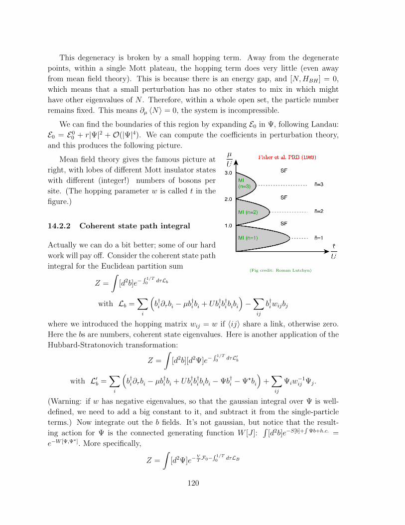
This degeneracy is broken by a small hopping term. Away from the degenerate
points, within a single Mott plateau, the hopping term does very little (even away
from mean field theory). This is because there is an energy gap, and [N,HBH ] = 0,
which means that a small perturbation has no other states to mix in which might
have other eigenvalues of N . Therefore, within a whole open set, the particle number
remains fixed. This means ∂µ 〈N〉 = 0, the system is incompressible.
We can find the boundaries of this region by expanding E0 in Ψ, following Landau:
E0 = E00 + r|Ψ|2 + O(|Ψ|4). We can compute the coefficients in perturbation theory,
and this produces the following picture.
(Fig credit: Roman Lutchyn)
Mean field theory gives the famous picture at
right, with lobes of different Mott insulator states
with different (integer!) numbers of bosons per
site. (The hopping parameter w is called t in the
figure.)
14.2.2 Coherent state path integral
Actually we can do a bit better; some of our hard
work will pay off. Consider the coherent state path
integral for the Euclidean partition sum
Z =
∫[d2b]e−
∫ 1/T0 dτLb
with Lb =∑i
(b†i∂τbi − µb
†ibi + Ub†ib
†ibibi
)−∑ij
b†iwijbj
where we introduced the hopping matrix wij = w if 〈ij〉 share a link, otherwise zero.
Here the bs are numbers, coherent state eigenvalues. Here is another application of the
Hubbard-Stratonovich transformation:
Z =
∫[d2b][d2Ψ]e−
∫ 1/T0 dτL′b
with L′b =∑i
(b†i∂τbi − µb
†ibi + Ub†ib
†ibibi −Ψb†i −Ψ?bi
)+∑ij
Ψiw−1ij Ψj.
(Warning: if w has negative eigenvalues, so that the gaussian integral over Ψ is well-
defined, we need to add a big constant to it, and subtract it from the single-particle
terms.) Now integrate out the b fields. It’s not gaussian, but notice that the result-
ing action for Ψ is the connected generating function W [J ]:∫
[d2b]e−S[b]+∫
Ψb+h.c. =
e−W [Ψ,Ψ?]. More specifically,
Z =
∫[d2Ψ]e−
VTF0−
∫ 1/T0 dτLB
120
with LB = K1Ψ?∂τΨ +K2|∂τΨ|2 +K3|~∇Ψ|2 + r|Ψ|2 + u|Ψ|4 + · · ·
Here V = Mad is the volume of space, and F0 is the mean-field free energy. The
coefficients K etc are connected Green’s functions of the bs. The choice of which terms
I wrote was dictated by Landau, and the order in which I wrote them should have been
determined by Wilson. The Mott-SF transition occurs when r changes sign, that is,
the condition r = 0 determines the location of the Mott-SF boundaries. You can see
that generically we have z = 2 kinetic terms. Less obvious is that r is proportional to
the mean field coefficient r.
Here’s the payoff. I claim that the coefficients in the action for Ψ are related by
K1 = −∂µr. (14.18)
This means that K1 = 0 precisely when the boundary of the lobe has a vertical tangent.
This means that right at those points (the ends of the dashed lines in the figure) the
second-order kinetic term is the leading one, and we have z = 1.
Here’s the proof of (14.18). LB must have the same symmetries as Lb. One such
invariance is
bi → bieiφ(τ), Ψi → Ψie
iφ(τ), µ→ µ+ i∂τφ.
This is a funny transformation which acts on the couplings, so doesn’t produce Noether
currents. It is still useful though, because it implies
0 = δφ(K1Ψ?∂τΨ + r|Ψ|2 + ...
)= K1|Ψ|2i∂τφ+ ∂µri∂φ|Ψ|2 + ...
14.2.3 Duality
We have seen above (in §14.1) that the prevention of vortices is essential to superfluidity,
which is the condensation of bosons. In D = 1 + 1, vortices are events in spacetime.
In D = 2 + 1, vortices are actual particles, i.e. localizable objects, around which the
superfluid phase variable winds by 2π (times an integer).
More explicitly, if the boson field which condenses is b(x) = veiφ, and we choose
polar coordinates in space x+ iy ≡ Reiϕ, then a vortex is a configuration of the order
parameter field of the form b(x) = f(R)eiϕ, where f(R)R→∞→ v far away: the phase
of the order parameter winds around. Notice that the phase is ill-defined in the core
of the vortex where f(R)R→0→ 0. (This is familiar from our discussion of the Abelian
Higgs model.)
To see the role of vortices in destroying superfluidity more clearly, consider super-
fluid flow in a 2d annulus geometry, with the same polar coordinates x+ iy = Reiϕ. If
121
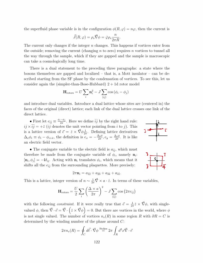
the superfluid phase variable is in the configuration φ(R,ϕ) = nϕ, then the current is
~J(R,ϕ) = ρs~∇φ = ϕρsn
2πR.
The current only changes if the integer n changes. This happens if vortices enter from
the outside; removing the current (changing n to zero) requires n vortices to tunnel all
the way through the sample, which if they are gapped and the sample is macroscopic
can take a cosmologically long time.
There is a dual statement to the preceding three paragraphs: a state where the
bosons themselves are gapped and localized – that is, a Mott insulator – can be de-
scribed starting from the SF phase by the condensation of vortices. To see this, let us
consider again the (simpler-than-Bose-Hubbard) 2 + 1d rotor model
Hrotors = U∑i
n2i − J
∑〈ij〉
cos (φi − φj)
and introduce dual variables. Introduce a dual lattice whose sites are (centered in) the
faces of the original (direct) lattice; each link of the dual lattice crosses one link of the
direct lattice.
• First let eij ≡φi−φj
2π. Here we define ij by the right hand rule:
ij× ij = +z (ij denotes the unit vector pointing from i to j). This
is a lattice version of ~e = z × ~∇φ 12π
. Defining lattice derivatives
∆xφi ≡ φi − φi+x, the definition is ex = −∆yφ
2π, ey = ∆xφ
2π. It is like
an electric field vector.
• The conjugate variable to the electric field is aij, which must
therefore be made from the conjugate variable of φi, namely ni:
[ni, φj] = −iδij. Acting with ni translates φi, which means that it
shifts all the eij from the surrounding plaquettes. More precisely:
2πni = a12 + a23 + a34 + a41.
This is a lattice, integer version of n ∼ 12π~∇× a · z. In terms of these variables,
Hrotors =U
2
∑i
(∆× a
2π
)2
− J∑〈ij〉
cos(2πeij
)with the following constraint. If it were really true that ~e = 1
2πz × ~∇φ, with single-
valued φ, then ~∇ · ~e = ~∇ ·(z × ~∇φ
)= 0. But there are vortices in the world, where φ
is not single valued. The number of vortices nv(R) in some region R with ∂R = C is
determined by the winding number of the phase around C:
2πnv(R) =
∮C
d~ · ~∇φ Stokes= 2π
∫R
d2x~∇ · ~e
122
(More explicitly, 2π~∇ · ~e = εzij∂i∂jφ = [∂x, ∂y]φ clearly vanishes if φ is single-valued.)
Since this is true for any region R, we have
~∇ · ~e = 2πδ2(vortices).
Actually, the lattice version of the equation has more information (and is true) because
it keeps track of the fact that the number of vortices is an integer:
∆xex + ∆yey ≡ ~∆ · ~e(i) = 2πnv (i), nv (i) ∈ Z.
It will not escape your notice that this is Gauss’ law, with the density of vortices playing
the role of the charge density.
Phases of the 2d rotors. Since ~e ∼ ~∇φ varies continuously, i.e. electric flux
is not quantized, this is called noncompact electrodynamics. Again we will impose
the integer constraint a ∈ 2πZ energetically, i.e. let a ∈ R and add (something like)
∆H?= −t cos a and see what happens when we make t finite. The expression in the
previous sentence is not quite right, yet, however: This operator does not commute
with our constraint ~∆ · ~e− 2πnv = 0 – it jumps ~e but not nv33.
We can fix this by introducing explicitly the variable which creates vortices, e−iχ,
with:
[nv (i), χ(j)] = −iδij .
Certainly our Hilbert space contains states with different number of vortices, so we
can introduce an operator which maps these sectors. Its locality might be an issue:
certainly it is nonlocal with respect to the original variables, but we will see that we
can treat it as a local operator (except for the fact that it carries gauge charge) in the
dual description. Since nv ∈ Z, χ ' χ+ 2π lives on a circle. So:
H ∼∑i
(U
2
(∆× a
2π
)2
+J
2(2πe)2 − t cos (∆χ− a)
)
still subject to the constraint ~∆ · ~e = 2πnv.
Two regimes:
J U, t : This suppresses e and its fluctuations, which means a fluctuates. The
fluctuating a is governed by the gaussian hamiltonian
H ∼∑(
~e2 +~b2)
33A set of words which has the same meaning as the above: cos a is not gauge invariant. Under-
standing these words requires us to think of the operator G(i) ≡ ~∆ · ~e − 2πnv as the generator of a
transformation,
δO =∑i
s(i)[G(i),O].
It can be a useful picture.
123
with b ≡ ∆×a2π
, which should look familiar. This deconfined phase has a gapless photon;
a 2 + 1d photon has a single polarization state. This is the goldstone mode, and this
regime describes the superfluid phase (note that the parameters work out right in the
original variables). The relation between the photon a and the original phase variable,
in the continuum is
εµνρ∂νaρ = ∂µφ.
t U, J : In this regime we must satisfy the cosine first. Like in D = 1 + 1,
this can be described as the statement that vortices condense. Expanding around its
minimum, the cosine term is
h 3 t (a− ∂χ)2
– the photon gets a mass by eating the phase variable χ. There is an energy gap. This
is the Mott phase.
If the vortices carry other quantum numbers, the (analog of the) Mott phase can
be more interesting, as we’ll see in section 14.3.
Compact electrodynamics in D = 2 + 1. Note that this free photon phase
of D = 2 + 1 electrodynamics is not accessible if e is quantized (so-called compact
electrodynamics) where monopole instantons proliferate and gap out the photon. This
is the subject of §14.2.5.
14.2.4 Particle-vortex duality in the continuum
The above is easier to understand (but a bit less precise) in the continuum. Consider a
quantum system of bosons in D = 2 + 1 with a U(1) particle-number symmetry (a real
symmetry, not a gauge redundancy). Let’s focus on a complex, non-relativistic bose
field b with action
S[b] =
∫dtd2x
(b†(i∂t − ~∇2 − µ
)b− U(b†b)2
). (14.19)
By Noether’s theorem, the symmetry b→ eiθb implies that the current
jµ = (jt,~j)µ = (b†b, ib†~∇b+ h.c.)µ
satisfies the continuity equation ∂µjµ = 0.
This system has two phases of interest here. In the ordered/broken/superfluid
phase, where the groundstate expectation value 〈b〉 =√ρ0 spontaneously breaks the
U(1) symmetry, the goldstone boson θ in b ≡ √ρ0eiθ is massless
Seff[θ] =ρ0
2
∫ (θ2 −
(~∇θ)2)
d2xdt, jµ = ρ0∂θ .
124
In the disordered/unbroken/Mott insulator phase, 〈b〉 = 0, and there is a mass gap. A
dimensionless parameter which interpolates between these phases is g = µ/U ; large g
encourages condensation of b.
We can ‘solve’ the continuity equation by writing
jµ = εµ··∂·a· (14.20)
where a· is a gauge potential. The time component of this equation says that the
boson density is represented by the magnetic flux of a. The spatial components relate
the boson charge current to the electric flux of a. The continuity equation for j is
automatic – it is the Bianchi identity for a – as long as a is single-valued. That is:
as long as there is no magnetic charge present. A term for this condition which is
commonly used in the cond-mat literature is: “a is non-compact.” (More on the other
case below.)
The relation (14.20) is the basic ingredient of the duality, but it is not a complete
description: in particular, how do we describe the boson itself in the dual variables?
In the disordered phase, adding a boson is a well-defined thing which costs a definite
energy. The boson is described by a localized clump of magnetic flux of a. Such a
configuration is energetically favored if a participates in a superconductor – i.e. if a is
coupled to a condensate of a charged field. The Meissner effect will then ensure that
its magnetic flux is bunched together. So this suggests that we should introduce into
the dual description a scalar field, call it Φ, minimally coupled to the gauge field a:
S[b]! Sdual[a,Φ] .
And the disordered phase should be dual to a phase where 〈Φ〉 6= 0, which gives a mass
to the gauge field by the Anderson-Higgs mechanism.
Who is Φ? More precisely, what is the identity in terms of the original bosons of
the particles it creates? When Φ is not condensed and its excitations are massive, the
gauge field is massless. This the Coulomb phase of the Abelian Higgs model S[a,Φ];
at low energies, it is just free electromagnetism in D = 2 + 1. These are the properties
of the ordered phase of b. (This aspect of the duality is explained in Wen, §6.3.) The
photon has one polarization state in D = 2 + 1 and is dual to the goldstone boson.
This is the content of (14.20) in the ordered phase: εµ··∂·a· = ρ0∂µθ or ?da = ρ0dθ.
Condensing Φ gives a mass to the Goldstone boson whose masslessness is guaranteed
by the broken U(1) symmetry. Therefore Φ is a disorder operator: its excitations
are vortices in the bose condensate, which are gapped in the superfluid phase. The
transition to the insulating phase can be described as a condensation of these vortices.
125
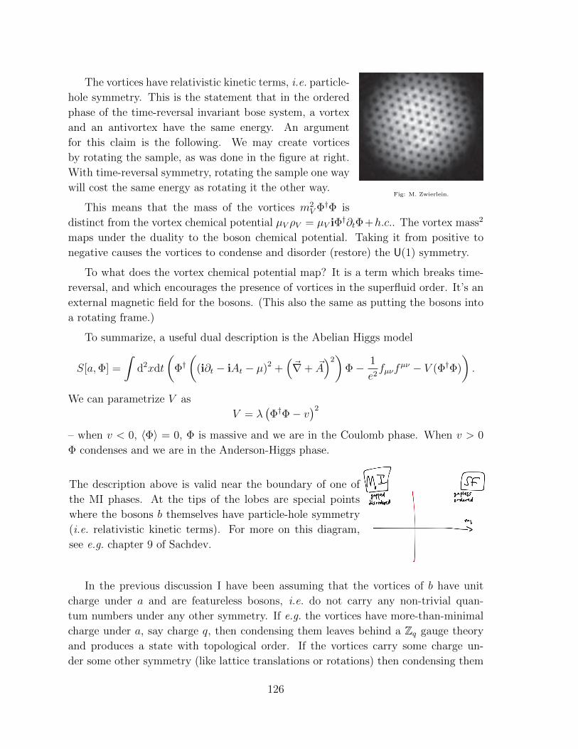
Fig: M. Zwierlein.
The vortices have relativistic kinetic terms, i.e. particle-
hole symmetry. This is the statement that in the ordered
phase of the time-reversal invariant bose system, a vortex
and an antivortex have the same energy. An argument
for this claim is the following. We may create vortices
by rotating the sample, as was done in the figure at right.
With time-reversal symmetry, rotating the sample one way
will cost the same energy as rotating it the other way.
This means that the mass of the vortices m2V Φ†Φ is
distinct from the vortex chemical potential µV ρV = µV iΦ†∂tΦ+h.c.. The vortex mass2
maps under the duality to the boson chemical potential. Taking it from positive to
negative causes the vortices to condense and disorder (restore) the U(1) symmetry.
To what does the vortex chemical potential map? It is a term which breaks time-
reversal, and which encourages the presence of vortices in the superfluid order. It’s an
external magnetic field for the bosons. (This also the same as putting the bosons into
a rotating frame.)
To summarize, a useful dual description is the Abelian Higgs model
S[a,Φ] =
∫d2xdt
(Φ†(
(i∂t − iAt − µ)2 +(~∇+ ~A
)2)
Φ− 1
e2fµνf
µν − V (Φ†Φ)
).
We can parametrize V as
V = λ(Φ†Φ− v
)2
– when v < 0, 〈Φ〉 = 0, Φ is massive and we are in the Coulomb phase. When v > 0
Φ condenses and we are in the Anderson-Higgs phase.
The description above is valid near the boundary of one of
the MI phases. At the tips of the lobes are special points
where the bosons b themselves have particle-hole symmetry
(i.e. relativistic kinetic terms). For more on this diagram,
see e.g. chapter 9 of Sachdev.
In the previous discussion I have been assuming that the vortices of b have unit
charge under a and are featureless bosons, i.e. do not carry any non-trivial quan-
tum numbers under any other symmetry. If e.g. the vortices have more-than-minimal
charge under a, say charge q, then condensing them leaves behind a Zq gauge theory
and produces a state with topological order. If the vortices carry some charge un-
der some other symmetry (like lattice translations or rotations) then condensing them
126
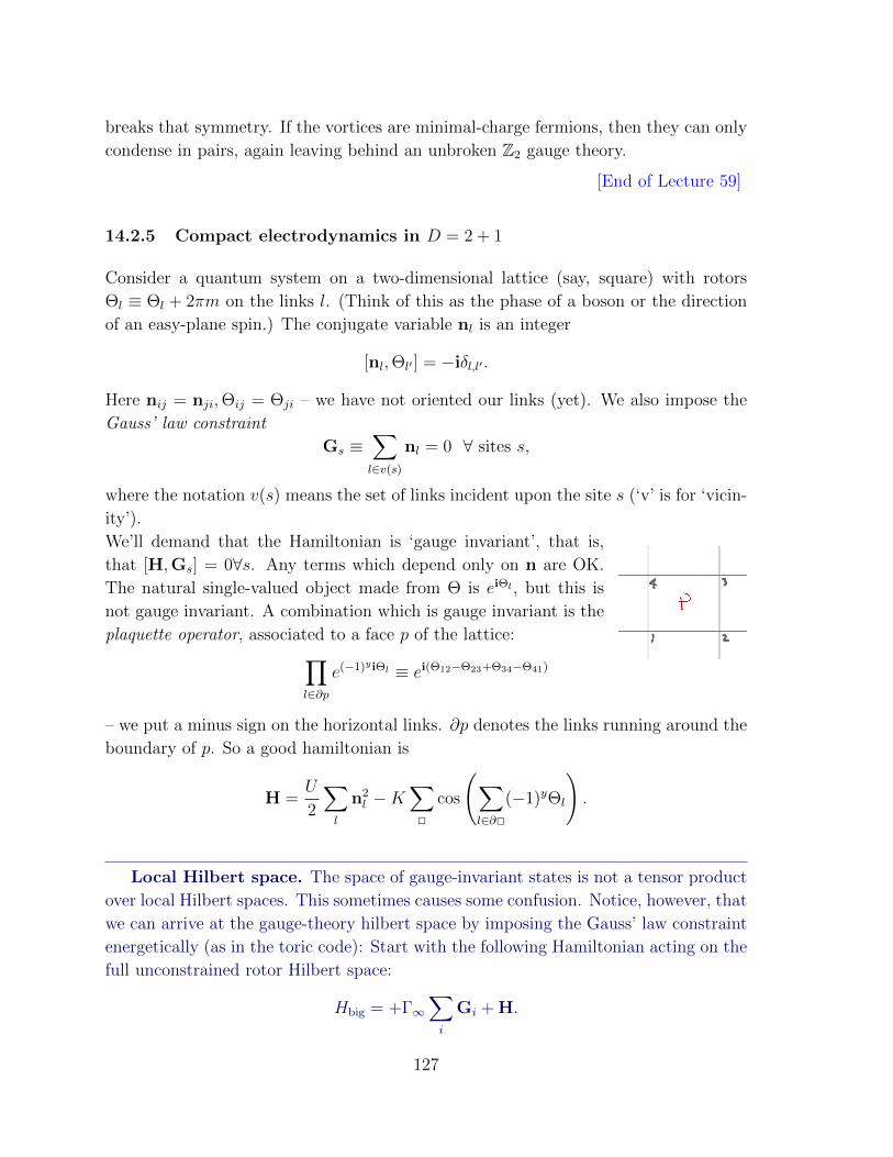
breaks that symmetry. If the vortices are minimal-charge fermions, then they can only
condense in pairs, again leaving behind an unbroken Z2 gauge theory.
[End of Lecture 59]
14.2.5 Compact electrodynamics in D = 2 + 1
Consider a quantum system on a two-dimensional lattice (say, square) with rotors
Θl ≡ Θl + 2πm on the links l. (Think of this as the phase of a boson or the direction
of an easy-plane spin.) The conjugate variable nl is an integer
[nl,Θl′ ] = −iδl,l′ .
Here nij = nji,Θij = Θji – we have not oriented our links (yet). We also impose the
Gauss’ law constraint
Gs ≡∑l∈v(s)
nl = 0 ∀ sites s,
where the notation v(s) means the set of links incident upon the site s (‘v’ is for ‘vicin-
ity’).
We’ll demand that the Hamiltonian is ‘gauge invariant’, that is,
that [H,Gs] = 0∀s. Any terms which depend only on n are OK.
The natural single-valued object made from Θ is eiΘl , but this is
not gauge invariant. A combination which is gauge invariant is the
plaquette operator, associated to a face p of the lattice:∏l∈∂p
e(−1)yiΘl ≡ ei(Θ12−Θ23+Θ34−Θ41)
– we put a minus sign on the horizontal links. ∂p denotes the links running around the
boundary of p. So a good hamiltonian is
H =U
2
∑l
n2l −K
∑2
cos
(∑l∈∂2
(−1)yΘl
).
Local Hilbert space. The space of gauge-invariant states is not a tensor product
over local Hilbert spaces. This sometimes causes some confusion. Notice, however, that
we can arrive at the gauge-theory hilbert space by imposing the Gauss’ law constraint
energetically (as in the toric code): Start with the following Hamiltonian acting on the
full unconstrained rotor Hilbert space:
Hbig = +Γ∞∑i
Gi + H.
127
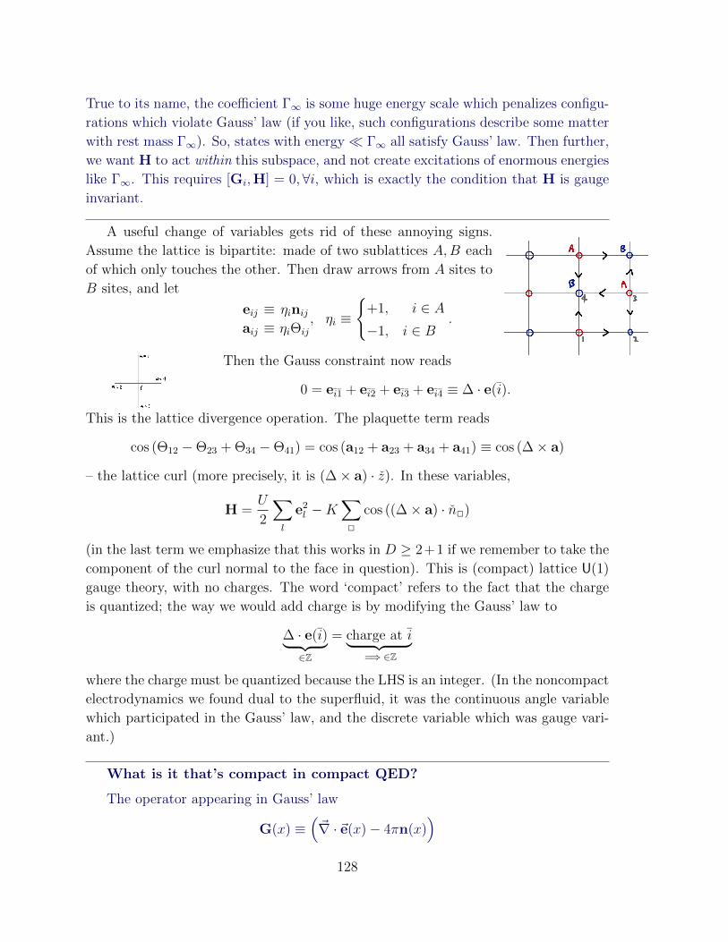
True to its name, the coefficient Γ∞ is some huge energy scale which penalizes configu-
rations which violate Gauss’ law (if you like, such configurations describe some matter
with rest mass Γ∞). So, states with energy Γ∞ all satisfy Gauss’ law. Then further,
we want H to act within this subspace, and not create excitations of enormous energies
like Γ∞. This requires [Gi,H] = 0,∀i, which is exactly the condition that H is gauge
invariant.
A useful change of variables gets rid of these annoying signs.
Assume the lattice is bipartite: made of two sublattices A,B each
of which only touches the other. Then draw arrows from A sites to
B sites, and let
eij ≡ ηinijaij ≡ ηiΘij
, ηi ≡
+1, i ∈ A−1, i ∈ B
.
Then the Gauss constraint now reads
0 = ei1 + ei2 + ei3 + ei4 ≡ ∆ · e(i).
This is the lattice divergence operation. The plaquette term reads
cos (Θ12 −Θ23 + Θ34 −Θ41) = cos (a12 + a23 + a34 + a41) ≡ cos (∆× a)
– the lattice curl (more precisely, it is (∆× a) · z). In these variables,
H =U
2
∑l
e2l −K
∑2
cos ((∆× a) · n2)
(in the last term we emphasize that this works in D ≥ 2+1 if we remember to take the
component of the curl normal to the face in question). This is (compact) lattice U(1)
gauge theory, with no charges. The word ‘compact’ refers to the fact that the charge
is quantized; the way we would add charge is by modifying the Gauss’ law to
∆ · e(i)︸ ︷︷ ︸∈Z
= charge at i︸ ︷︷ ︸=⇒ ∈Z
where the charge must be quantized because the LHS is an integer. (In the noncompact
electrodynamics we found dual to the superfluid, it was the continuous angle variable
which participated in the Gauss’ law, and the discrete variable which was gauge vari-
ant.)
What is it that’s compact in compact QED?
The operator appearing in Gauss’ law
G(x) ≡(~∇ · ~e(x)− 4πn(x)
)128
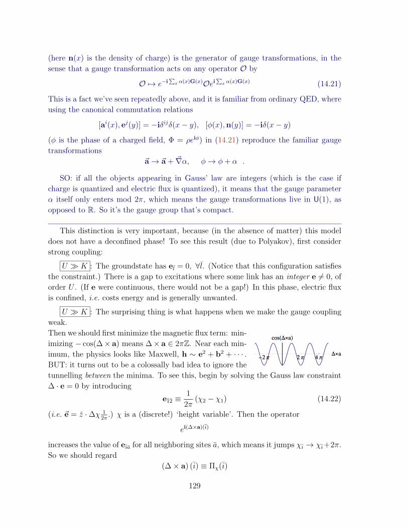
(here n(x) is the density of charge) is the generator of gauge transformations, in the
sense that a gauge transformation acts on any operator O by
O 7→ e−i∑x α(x)G(x)Oei
∑x α(x)G(x) (14.21)
This is a fact we’ve seen repeatedly above, and it is familiar from ordinary QED, where
using the canonical commutation relations
[ai(x), ej(y)] = −iδijδ(x− y), [φ(x),n(y)] = −iδ(x− y)
(φ is the phase of a charged field, Φ = ρeiφ) in (14.21) reproduce the familiar gauge
transformations
~a→ ~a + ~∇α, φ→ φ+ α .
SO: if all the objects appearing in Gauss’ law are integers (which is the case if
charge is quantized and electric flux is quantized), it means that the gauge parameter
α itself only enters mod 2π, which means the gauge transformations live in U(1), as
opposed to R. So it’s the gauge group that’s compact.
This distinction is very important, because (in the absence of matter) this model
does not have a deconfined phase! To see this result (due to Polyakov), first consider
strong coupling:
U K : The groundstate has el = 0, ∀l. (Notice that this configuration satisfies
the constraint.) There is a gap to excitations where some link has an integer e 6= 0, of
order U . (If e were continuous, there would not be a gap!) In this phase, electric flux
is confined, i.e. costs energy and is generally unwanted.
U K : The surprising thing is what happens when we make the gauge coupling
weak.
Then we should first minimize the magnetic flux term: min-
imizing − cos(∆× a) means ∆× a ∈ 2πZ. Near each min-
imum, the physics looks like Maxwell, h ∼ e2 + b2 + · · · .BUT: it turns out to be a colossally bad idea to ignore the
tunnelling between the minima. To see this, begin by solving the Gauss law constraint
∆ · e = 0 by introducing
e12 ≡1
2π(χ2 − χ1) (14.22)
(i.e. ~e = z ·∆χ 12π
.) χ is a (discrete!) ‘height variable’. Then the operator
ei(∆×a)(i)
increases the value of eia for all neighboring sites a, which means it jumps χi → χi+2π.
So we should regard
(∆× a) (i) ≡ Πχ(i)
129
as the conjugate variable to χ, in the sense that
[Πχ(r), χ(r′)] = −iδrr′ .
Notice that this is consistent with thinking of χ as the dual scalar related to the
gauge field by our friend the (Hodge) duality relation
∂µχ = εµνρ∂νaρ.
The spatial components i say ∂iχ = εijf0j, which is the continuum version of (14.22).
The time component says χ = εijfij = ∇×a, which indeed says that (if χ has quadratic
kinetic terms), the field momentum of χ is the magnetic flux. So χ is the would-be
transverse photon mode.
The hamiltonian is now
H =U
2
∑l
(∆χ)2 −K∑r
cos Πχ(r)
with no constraint. In the limit U K, the spatial gradients of χ are forbidden –
χ wants to be uniform. From the definition (14.22), uniform χ means there are no
electric field lines, this is the confined phase. Deconfinement limit should be K U ,
in which case it looks like we can Taylor expand the cosine cos Πχ ∼ 1− 12Π2χ about one
of its minima, and get harmonic oscillators. But: tunneling between the neighboring
vacua of ∆× a is accomplished by the flux-insertion operator (or monopole operator)
eiχ, which satisfies [eiχ(r), (∆× a) (r′)] = eiχ(r)δrr′
– that is, eiχ is a raising operator for ∆ × a. To analyze whether the Maxwell limit
survives this, let’s go to the continuum and study perturbations of the free hamiltonian
H0 =
∫ (U
2
(~∇χ)2
+K
2Π2χ
)by
H1 = −∫V0 cosχ .
This operator introduces tunneling events by Πχ → Φχ±2π with rate V0. Alternatively,
notice that again we can think of the addition of this term as energetically imposing
the condition that χ ∈ 2πZ.
So: is V0 irrelevant? Very much no. In fact
〈cosχ(r) cosχ(0)〉0 ∼ const (14.23)
130
has constant amplitude at large r! That means that the operator has dimension zero,
and the perturbation in the action has [S1 = −∫V0 cosχd2xdτ ] ∼ L3, very relevant.
The result is that it pins the χ field (the would-be photon mode) to an integer, from
which it can’t escape. This result is due to Polyakov.
To see (14.23) begin with the gaussian identity⟨eisχ(x)eis′χ(0)
⟩= e−
ss′2〈χ(x)χ(0)〉 ,
with s, s′ = ±. The required object is
〈χ(x)χ(0)〉 =i
T
∫d3p
ei~p·~x
p2= i
2π
(2π)3T
∫ ∞0
dp
∫ 1
−1
d cos θeipx cos θ︸ ︷︷ ︸= 2 sin px
px
= i2
(2π)2T
∫ ∞0
dpsin px
px
= i2
2πT
1
x
1
2
∫ ∞−∞
dpsin p
p︸ ︷︷ ︸=π
=i
2Tx. (14.24)
(I have set the velocity of propagation to 1, and T ≡ U/K is the coefficient in front of
the Lagrangian, S = T∫d3x∂µχ∂
µχ.) So⟨eisχ(x)eis′χ(0)
⟩= e−i ss
′4xT .
And
〈cosχ(x) cosχ(0)〉 = cos1
4Txwhich does not decay at long distance, and in fact approaches a constant.
• The fact that the would-be-transverse-photon χ is massive means confinement of
the gauge theory. To see that external charge is confined, think as usual about
the big rectangular Wilson loop 〈W (2)〉 =⟨ei∮
2 A⟩ euclidean∼ e−E(R)T as an order
parameter for confinement. In term of χ,∮2A =
∫F12 =
∫gχ
(I’ve absorbed a factor of the gauge coupling into χ to make the dimensions work
nicely, εµνρ∂νAρ = g∂µχ) and the expectation is
〈W (2)〉 = Z−1
∫[dχ]e−Sχ+gi
∫ χ ∼ e−cg
2mχ·area().
131
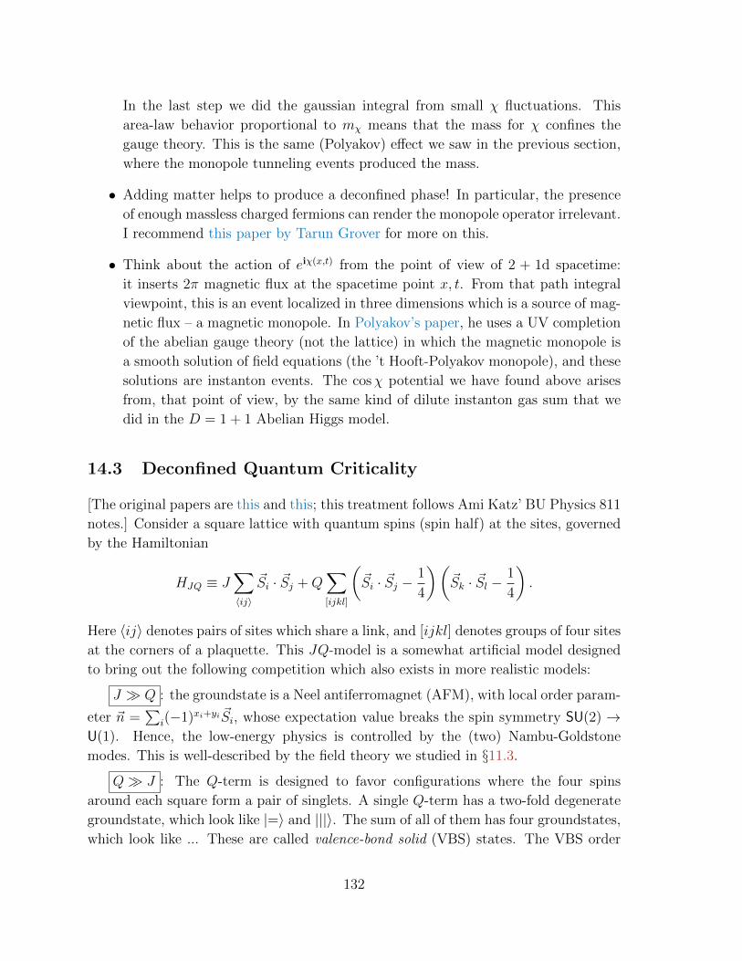
In the last step we did the gaussian integral from small χ fluctuations. This
area-law behavior proportional to mχ means that the mass for χ confines the
gauge theory. This is the same (Polyakov) effect we saw in the previous section,
where the monopole tunneling events produced the mass.
• Adding matter helps to produce a deconfined phase! In particular, the presence
of enough massless charged fermions can render the monopole operator irrelevant.
I recommend this paper by Tarun Grover for more on this.
• Think about the action of eiχ(x,t) from the point of view of 2 + 1d spacetime:
it inserts 2π magnetic flux at the spacetime point x, t. From that path integral
viewpoint, this is an event localized in three dimensions which is a source of mag-
netic flux – a magnetic monopole. In Polyakov’s paper, he uses a UV completion
of the abelian gauge theory (not the lattice) in which the magnetic monopole is
a smooth solution of field equations (the ’t Hooft-Polyakov monopole), and these
solutions are instanton events. The cosχ potential we have found above arises
from, that point of view, by the same kind of dilute instanton gas sum that we
did in the D = 1 + 1 Abelian Higgs model.
14.3 Deconfined Quantum Criticality
[The original papers are this and this; this treatment follows Ami Katz’ BU Physics 811
notes.] Consider a square lattice with quantum spins (spin half) at the sites, governed
by the Hamiltonian
HJQ ≡ J∑〈ij〉
~Si · ~Sj +Q∑[ijkl]
(~Si · ~Sj −
1
4
)(~Sk · ~Sl −
1
4
).
Here 〈ij〉 denotes pairs of sites which share a link, and [ijkl] denotes groups of four sites
at the corners of a plaquette. This JQ-model is a somewhat artificial model designed
to bring out the following competition which also exists in more realistic models:
J Q : the groundstate is a Neel antiferromagnet (AFM), with local order param-
eter ~n =∑
i(−1)xi+yi ~Si, whose expectation value breaks the spin symmetry SU(2) →U(1). Hence, the low-energy physics is controlled by the (two) Nambu-Goldstone
modes. This is well-described by the field theory we studied in §11.3.
Q J : The Q-term is designed to favor configurations where the four spins
around each square form a pair of singlets. A single Q-term has a two-fold degenerate
groundstate, which look like |=〉 and |||〉. The sum of all of them has four groundstates,
which look like ... These are called valence-bond solid (VBS) states. The VBS order
132
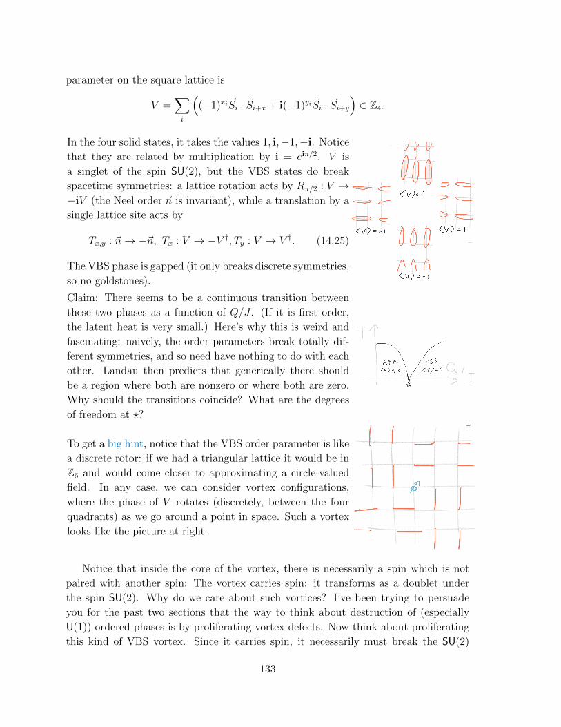
parameter on the square lattice is
V =∑i
((−1)xi ~Si · ~Si+x + i(−1)yi ~Si · ~Si+y
)∈ Z4.
In the four solid states, it takes the values 1, i,−1,−i. Notice
that they are related by multiplication by i = eiπ/2. V is
a singlet of the spin SU(2), but the VBS states do break
spacetime symmetries: a lattice rotation acts by Rπ/2 : V →−iV (the Neel order ~n is invariant), while a translation by a
single lattice site acts by
Tx,y : ~n→ −~n, Tx : V → −V †, Ty : V → V †. (14.25)
The VBS phase is gapped (it only breaks discrete symmetries,
so no goldstones).
Claim: There seems to be a continuous transition between
these two phases as a function of Q/J . (If it is first order,
the latent heat is very small.) Here’s why this is weird and
fascinating: naively, the order parameters break totally dif-
ferent symmetries, and so need have nothing to do with each
other. Landau then predicts that generically there should
be a region where both are nonzero or where both are zero.
Why should the transitions coincide? What are the degrees
of freedom at ??
To get a big hint, notice that the VBS order parameter is like
a discrete rotor: if we had a triangular lattice it would be in
Z6 and would come closer to approximating a circle-valued
field. In any case, we can consider vortex configurations,
where the phase of V rotates (discretely, between the four
quadrants) as we go around a point in space. Such a vortex
looks like the picture at right.
Notice that inside the core of the vortex, there is necessarily a spin which is not
paired with another spin: The vortex carries spin: it transforms as a doublet under
the spin SU(2). Why do we care about such vortices? I’ve been trying to persuade
you for the past two sections that the way to think about destruction of (especially
U(1)) ordered phases is by proliferating vortex defects. Now think about proliferating
this kind of VBS vortex. Since it carries spin, it necessarily must break the SU(2)
133
symmetry, as the Neel phase does. This is why the transitions happen at the same
point.
To make this more quantitative, let’s think about it from the AFM side: how do
we make V from the degrees of freedom of the low energy theory? It’s not made from
n since it’s a spin singlet which isn’t 1 (spin singlets made from n are even under a
lattice translation). What about the CP1 version, aka the Abelian Higgs model, aka
scalar QED (now in D = 2 + 1)?
L = − 1
4g2F 2 + |Dz|2 −m2|z|2 − λ
4|z|4
where z =
(z↑z↓
), and Dµz = (∂µ− iAµ)z as usual. Let’s think about the phases of this
model.
m2 < 0 : Here z condenses and breaks SU(2)→ U(1), and Aµ is higgsed. A gauge
invariant order parameter is ~n = z†~σz, and there are two goldstones associated with
its rotations. This is the AFM. The cautionary tale I told you about this phase in
D = 1 + 1 doesn’t happen because now the vortices are particles rather than instanton
events. More on these particles below.
m2 > 0 : Naively, in this phase, z are uncondensed and massive, leaving at low
energies only Llow-E?= − 1
4g2F2, Maxwell theory in D = 2 + 1. This looks innocent
but it will occupy us for quite a few pages starting now. This model has a conserved
current (conserved by the Bianchi identity)
JµF ≡ εµνρFνρ.
The thing that’s conserved is the lines of magnetic flux. We can follow these more
effectively by introducing the dual scalar field by a by-now-familiar duality relation:
JµF ≡ εµνρFνρ ≡ g∂µχ. (14.26)
You can think of the last equation here as a solution of the conservation law ∂µJµF = 0.
The symmetry acts on χ by shifts: χ → χ + constant. In terms of χ, the Maxwell
action is
Llow-E?= − 1
4g2F 2 =
1
2∂µχ∂
µχ.
But this is a massless scalar, a gapless theory. And what is the χ → χ + c symmetry
in terms of the spin system? I claim that it’s the rotation of the phase of the VBS
order parameter, which is explicitly broken by the squareness of the square lattice. An
improvement would then be
Llow-E =1
2∂µχ∂
µχ− 1
2m2χχ
2 + · · ·
134
where mχ ∼ 1a2 comes from the lattice breaking the rotation invariance (a is the lattice
spacing).
To see that shifts of χ are VBS rotations, let’s reproduce the lattice symmetries in
the Abelian Higgs model. Here’s the action of lattice translations T ≡ Tx or Ty (take
a deep breath.): T : na → −na but na = z†σaz, so on z we must have T : z → iσ2z?.
The gauge current is jµ = iz†∂µz + h.c.→ −jµ which means we must have Aµ → −Aµand Fµν → −Fµν . Therefore by (14.26) we must have T : ∂χ → −∂χ which means
that
Tx,y : χ→ −χ+ gαx,y
where αx,y are some so-far-undetermined numbers, and g is there on dimensional
grounds. Therefore, by choosing Tx,yχ → −χ ± gπ/2, Rπ/2 : χ → χ − gπ/2 we can
reproduce the transformation (14.25) by identifying
V = ceiχ/g
(up to an undetermined overall complex number). Notice for future reference the
canonical commutation relation between the flux current density (J0F = gχ = g
iδδχ
) and
V :
[J0F (x), V (0)] = V (0)δ2(x). (14.27)
It creates flux.
So χ is like the phase of the bosonic operator V which is condensed in the VBS
phase; lattice effects break the U(1) symmetry down to some discrete subgroup (Z4 for
the square lattice, Z6 for triangular, Z3 for honeycomb), with a potential of the form
V(V k) = m3χ cos(4χ/g) + · · · , where k = 4, 6, 3... depends on the lattice, which has k
minima, corresponding to the k possible VBS states. By (14.27), such a potential has
charge k under JF .
Consider this phase from the point of view of the gauge theory now. Notice that χ
is the same (up to a factor) dual variable we introduced in our discussion of compact
QED, and the Wilson loop will again produce an area law if χ is massive, as with the
Polyakov effect.
In order for this story to make sense, we need that M, g2 1a2 , so that χ is actually
a low-energy degree of freedom. The idea is that the critical point from tuning J/Q
to the critical value is reached by taking mχ → 0. What is the nature of this critical
theory? It has emergent deconfined gauge fields, even though the phases on either side
of the critical point do not (they are confined m > 0 and Higgsed m < 0 respectively).
Hence the name deconfined quantum criticality.
The conjecture (which would explain the phase diagram above) is that this gauge
theory is a critical theory (in fact a conformal field theory) with only one relevant
135
operator (the one which tunes us through the phase transition, the mass for χ) which
is a singlet under all the symmetries. Recall that eikχ has charge k under the JFsymmetry, and the square lattice preserves a Z4 ⊂ U(1) subgroup, so only allows the 4-
vortex-insertion operator ei4χ. What is the dimension of this operator? The conjecture
is that it has dimension larger than 3.
[End of Lecture 60]
Insanely brief sketch of a check at large N . Actually, this can be checked very
explicitly in a large-N version of the model, with N component z fields, so that the spin
is φA = z†TAz, A = 1..N2 − 1. This has SU(N) symmetry. When m2 < 0, it is broken
to SU(N − 1), with 2(N − 1) goldstone bosons. (Actually there is a generalization of
the lattice model which realizes this – just make the spins into N ×N matrices.)
Introducing an H-S field σ to decouple the |z|4 interaction, we can make the z
integrals gaussian, and find (this calculation is just like our earlier analysis in §11.3.4)
S[A, σ] =
∫dp
(1
4Fµν(p)
(1
g2UV
+c1N
iplog
2m+ ip
2m− ip
)F µν(−p) + σ(p)
(−1
λ+c2N
iplog
2m+ ip
2m− ip
)σ(−p)
)In the IR limit, m p g2
UVN, λN , this is a scale-invariant theory with 〈FF 〉 ∼p, 〈σσ〉 ∼ p so that both F and σ have dimension near 2. (Actually the dimension of F
is fixed at 2 by flux conservation.) z doesn’t get any anomalous dimension at leading
order in N .
This is all consistent with the claim so far. What is the dimension of V4 = ei4χ?
To answer this question, we use a powerful tool of conformal field theory called radial
quantization. Consider the theory on a cylinder, S2 × R, where the last factor we can
interpret as time. In a conformal field theory there is a one-to-one map between local
operators and states of the theory on Sd ×R. The state corresponding to an operator
O is just O(0) |0〉. The energy of the state on the sphere is the scaling dimension of
the operator. (For an explanation of this, I refer to §4 of these notes.)
The state created by acting with Vk(0) on the vacuum maps by this transformation
to an initial state with flux k spread over the sphere (think of it as the 2-sphere
surrounding the origin in spacetime): this state has charge k under QF =∫S2 J
0F =∫
S2 F12. The dimension of Vk is the energy of the lowest-energy state with QF = k. We
can compute this by euclidean-time path integral:
Zk = trQF=ke−THcyl
T→∞→ e−T∆k .
This is
Zk =
∫[dA]δ
(∫F − k
)∫[dzdz†]e−S[z,A] ≡ e−Fk
136
which at large-N we can do by saddle point. The dominant configuration of the gauge
field is the charge-k magnetic monopole Aϕ = k2(1− cosϕ), and we must compute∫
[d2z]ez†(−D†ADA+m2)z = det
(−D†ADA +m2
)−N/2= e−
N2
tr log(−D†ADA+m2)
The free energy is then a sum over eigenstates of this operator(−∂2
τ − ~D2A
)f`e
iωτ =(ω2 + λ`(k)
)f`e
iωτ
Fk = NT
∫dω∑`
(2`+ 1) log(ω2 + λ`(k) +m2).
The difference Fk − F0 is UV finite and gives ∆k = Nck, c1 ∼ .12, c4 ∼ .82. Unitary
requires ∆1 ≥ 12
(= the free scalar dimension), so don’t trust this for N < 4.
Pure field theory description. We’ve been discussing a theory with U(1)VBS ×SU(2)spin symmetry. Lattice details aside, how can we encode the way these two
symmetries are mixed up which forces the order parameter of one to be the disor-
der operator for the other? To answer this, briefly consider enlarging the symmetry
to SO(5) ⊂ U(1)VBS × SU(2)spin, and organize (ReV, ImV, n1, n2, n3) ≡ na into a 5-
component mega-voltron-spin vector. We saw that in D = 0 + 1, we could make a
WZW term with a 3-component spin
W0[(n1, n2, n3)] =
∫B2
εabcnadnb ∧ dnc.
Its point in life was to impose the spin commutation relations at spin s when the
coefficient is 2s. In D = 1 + 1, we can make a WZW term with a 4-component spin,
which can have SO(4) symmetry
W1[(n1, n2, n3, n4)] =
∫B3
εabcdnadnb ∧ dnc ∧ dnd.
34 Once we’ve got this far, how can you resist considering
W2[(n1, n2, n3, n4, n5)] =
∫B4
εabcdenadnb ∧ dnc ∧ dnd ∧ dne.
34In fact the D = 1 + 1 version of this is extremely interesting. A few brief comments: (1) involves
a real VBS order parameter n4.) (2) The D = 1 + 1 term has the same number of derivatives (in
the EOM) as the kinetic term ∂na∂na. This means they can compete at a fixed point. The resulting
CFTs are called WZW models. (3) The above is in fact a description of the spin-half chain, which
previously we’ve described by an O(3) sigma model at θ = π.
137
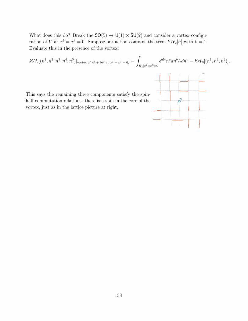
What does this do? Break the SO(5) → U(1) × SU(2) and consider a vortex configu-
ration of V at x2 = x3 = 0. Suppose our action contains the term kW2[n] with k = 1.
Evaluate this in the presence of the vortex:
kW2[(n1, n2, n3, n4, n5)|vortex of n1 + in2 at x2 = x3 = 0] =
∫B2|x2=x3=0
εabcnadnb∧dnc = kW0[(n1, n2, n3)].
This says the remaining three components satisfy the spin-
half commutation relations: there is a spin in the core of the
vortex, just as in the lattice picture at right.
138
15 Effective field theory
[Some nice lecture notes on effective field theory can be found here: J. Polchinski,
A. Manohar, D. B. Kaplan, H. Georgi.]
Diatribe about ‘renormalizability’. Having internalized Wilson’s perspective
on renormalization – namely that we should include all possible operators consistent
with symmetries and let the dynamics decide which are important at low energies – we
are led immediately to the idea of an effective field theory (EFT). There is no reason to
demand that a field theory that we have found to be relevant for physics in some regime
should be a valid description of the world to arbitrarily short (or long!) distances. This
is a happy statement: there can always be new physics that has been so far hidden
from us. Rather, an EFT comes with a regime of validity, and with necessary cutoffs.
As we will discuss, in a useful implementation of an EFT, the cutoff implies a small
parameter in which we can expand (and hence compute).
Caring about renormalizibility is pretending to know about physics at arbitrarily
short distances. Which you don’t.
Even when theories are renormalizable, this apparent victory is often false. For
example, QED requires only two independent counterterms (mass and charge of the
electron), and is therefore by the old-fashioned definition renormalizable, but it is
superseded by the electroweak theory above 80GeV. Also: the coupling in QED actually
increases logarithmically at shorter distances, and ultimately reaches a Landau pole
at SOME RIDICULOUSLY HIGH ENERGY (of order e+ cα where α ∼ 1
137is the fine
structure constant (e.g. at the scale of atomic physics) and c is some numerical number.
Plugging in numbers gives something like 10330 GeV, which is quite a bit larger than the
Planck scale). This is of course completely irrelevant for physics and even in principle
because of the previous remark about electroweak unification. And if not because of
that, because of the Planck scale. A heartbreaking historical fact is that Landau and
many other smart people gave up on QFT as a whole because of this silly fantasy about
QED in an unphysical regime.
We will see below that even in QFTs which are non-renormalizable in the strict
sense, there is a more useful notion of renormalizability: effective field theories come
with a parameter (often some ratio of mass scales), in which we may expand the action.
A useful EFT requires a finite number of counterterms at each order in the expansion.
Furthermore, I claim that this is always the definition of renormalizability that
we are using, even if we are using a theory which is renormalizable in the traditional
sense, which allows us to pretend that there is no cutoff. That is, there could always
be corrections of order(
EEnew
)nwhere E is some energy scale of physics that we are
139
doing and Enew is some UV scale where new physics might come in; for large enough
n, this is too small for us to have seen. The property of renormalizibility that actually
matters is that we need a finite number of counterterms at each order in the expansion
in EEnew
.
Renormalizable QFTs are in some sense less powerful than non-renormalizable ones
– the latter have the decency to tell us when they are giving the wrong answer! That
is, they tell us at what energy new physics must come in; with a renormalizable theory
we may blithely pretend that it is valid in some ridiculously inappropriate regime like
10330 GeV.
Notions of EFT. There is a dichotomy in the way EFTs are used. Sometimes one
knows a lot about the UV theory (e.g.
• electroweak gauge theory,
• QCD,
• electrons in a solid,
• water molecules
...) but it is complicated and unwieldy for the questions one wants to answer, so instead
one develops an effective field theory involving just the appropriate and important dofs
(e.g., respectively,
• Fermi theory of weak interactions,
• chiral lagrangian (or HQET or SCET or ...),
• Landau Fermi liquid theory (or the Hubbard model or a topological field theory
or ...),
• hydrodynamics (or some theory of phonons in ice or ...)
...). As you can see from the preceding lists of examples, even a single UV theory
can have many different IR EFTs depending on what phase it is in, and depending on
what question one wants to ask. The relationship between the pairs of theories above
is always coarse-graining from the UV to the IR, though exactly what plays the role
of the RG parameter can vary wildly. For example, in the example of the Fermi liquid
theory, the scaling is ω → 0, and momenta scale towards the Fermi surface, not ~k = 0.
A second situation is when one knows a description of some low-energy physics up
to some UV scale, and wants to try to infer what the UV theory might be. This is a
140
common situation in physics! Prominent examples include: the Standard Model, and
quantized Einstein gravity. Occasionally we (humans) actually learn some physics and
an example of an EFT from the second category moves to the first category.
Summary of basic EFT logic. Answer the following questions:
1. what are the dofs?
2. what are the symmetries?
3. where is the cutoff on its validity?
Then write down all interactions between the dofs which preserve the symmetry in an
expansion in derivatives, with higher-dimension operators suppressed by more powers
of the UV scale.
I must also emphasize two distinct usages of the term ‘effective field theory’ which
are common, and which the discussion above is guilty of conflating (this (often slip-
pery) distinction is emphasized in the review article by Georgi linked at the beginning
of this subsection). The Wilsonian perspective advocated above produces a low-energy
description of the physics which is really just a way of solving (if you can) the original
model; very reductively, it’s just a physically well-motivated order for doing the inte-
grals. If you really integrate out the high energy modes exactly, you will get a non-local
action for the low energy modes. This is to be contrasted with the local actions one
uses in practice, by truncating the derivative expansion. It is the latter which is really
the action of the effective field theory, as opposed to the full theory, with some of the
integrals done already. The latter will give correct answers for physics below the cutoff
scale, and it will give them much more easily.
Some interesting and/or important examples of EFT that we will not discuss ex-
plicitly, and where you can learn about them:
• Hydrodynamics [Kovtun]
• Fermi liquid theory [J. Polchinski, R. Shankar, Rev. Mod. Phys. 66 (1994) 129]
• chiral perturbation theory [D. B. Kaplan, §4]
• heavy quark effective field theory [D. B. Kaplan, §1.3]
• random surface growth (KPZ) [Zee, chapter VI]
141
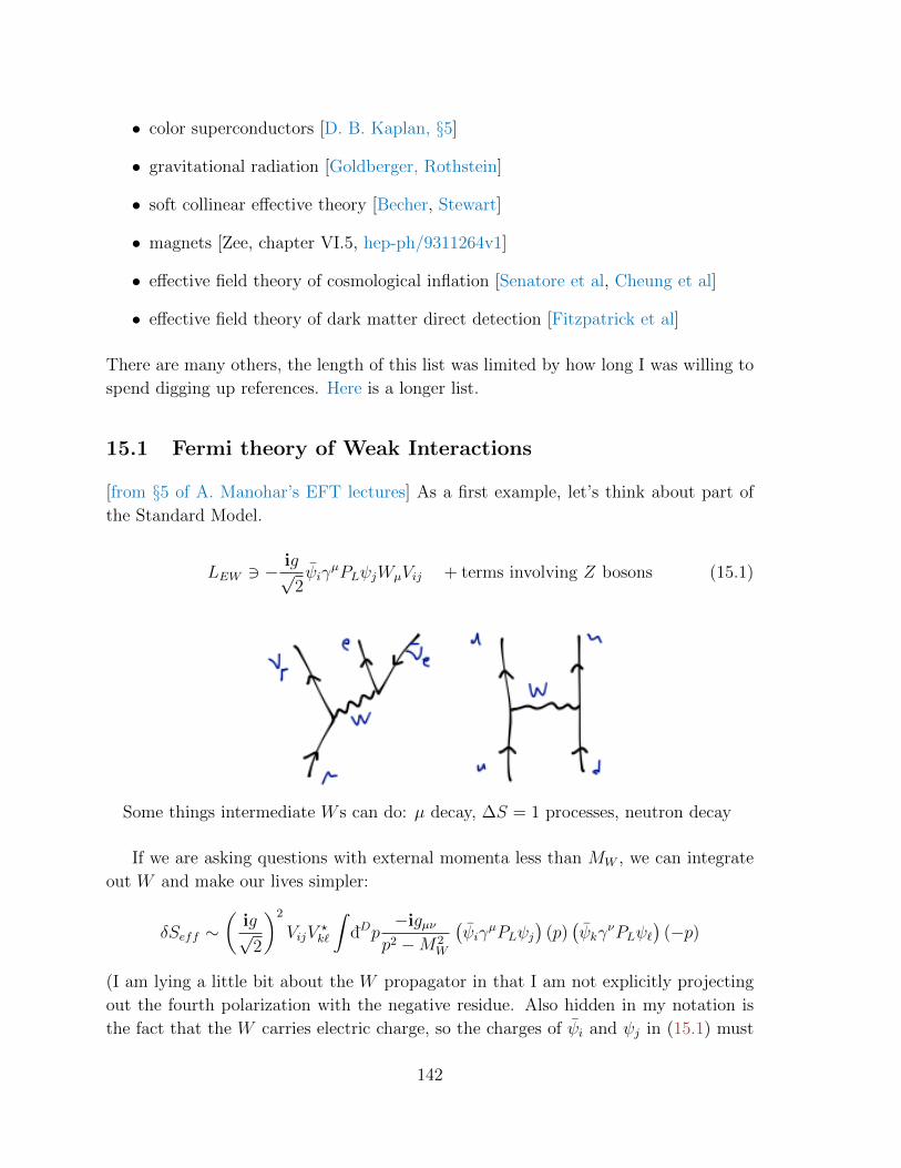
• color superconductors [D. B. Kaplan, §5]
• gravitational radiation [Goldberger, Rothstein]
• soft collinear effective theory [Becher, Stewart]
• magnets [Zee, chapter VI.5, hep-ph/9311264v1]
• effective field theory of cosmological inflation [Senatore et al, Cheung et al]
• effective field theory of dark matter direct detection [Fitzpatrick et al]
There are many others, the length of this list was limited by how long I was willing to
spend digging up references. Here is a longer list.
15.1 Fermi theory of Weak Interactions
[from §5 of A. Manohar’s EFT lectures] As a first example, let’s think about part of
the Standard Model.
LEW 3 −ig√
2ψiγ
µPLψjWµVij + terms involving Z bosons (15.1)
Some things intermediate W s can do: µ decay, ∆S = 1 processes, neutron decay
If we are asking questions with external momenta less than MW , we can integrate
out W and make our lives simpler:
δSeff ∼(
ig√2
)2
VijV?k`
∫dDp
−igµνp2 −M2
W
(ψiγ
µPLψj)
(p)(ψkγ
νPLψ`)
(−p)
(I am lying a little bit about the W propagator in that I am not explicitly projecting
out the fourth polarization with the negative residue. Also hidden in my notation is
the fact that the W carries electric charge, so the charges of ψi and ψj in (15.1) must
142
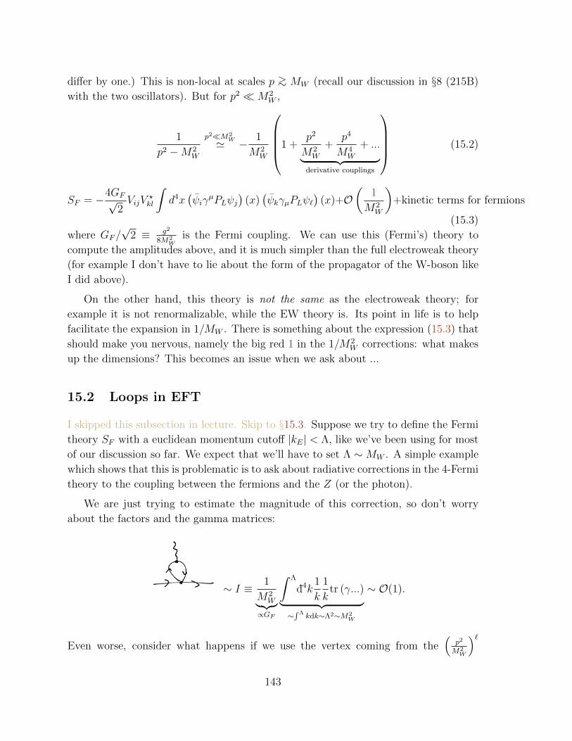
differ by one.) This is non-local at scales p >∼ MW (recall our discussion in §8 (215B)
with the two oscillators). But for p2 M2W ,
1
p2 −M2W
p2M2W' − 1
M2W
1 +p2
M2W
+p4
M4W
+ ...︸ ︷︷ ︸derivative couplings
(15.2)
SF = −4GF√2VijV
?kl
∫d4x
(ψiγ
µPLψj)
(x)(ψkγµPLψ`
)(x)+O
(1
M2W
)+kinetic terms for fermions
(15.3)
where GF/√
2 ≡ g2
8M2W
is the Fermi coupling. We can use this (Fermi’s) theory to
compute the amplitudes above, and it is much simpler than the full electroweak theory
(for example I don’t have to lie about the form of the propagator of the W-boson like
I did above).
On the other hand, this theory is not the same as the electroweak theory; for
example it is not renormalizable, while the EW theory is. Its point in life is to help
facilitate the expansion in 1/MW . There is something about the expression (15.3) that
should make you nervous, namely the big red 1 in the 1/M2W corrections: what makes
up the dimensions? This becomes an issue when we ask about ...
15.2 Loops in EFT
I skipped this subsection in lecture. Skip to §15.3. Suppose we try to define the Fermi
theory SF with a euclidean momentum cutoff |kE| < Λ, like we’ve been using for most
of our discussion so far. We expect that we’ll have to set Λ ∼MW . A simple example
which shows that this is problematic is to ask about radiative corrections in the 4-Fermi
theory to the coupling between the fermions and the Z (or the photon).
We are just trying to estimate the magnitude of this correction, so don’t worry
about the factors and the gamma matrices:
∼ I ≡ 1
M2W︸︷︷︸
∝GF
∫ Λ
d4k1
k
1
ktr (γ...)︸ ︷︷ ︸
∼∫ Λ kdk∼Λ2∼M2
W
∼ O(1).
Even worse, consider what happens if we use the vertex coming from the(
p2
M2W
)`143
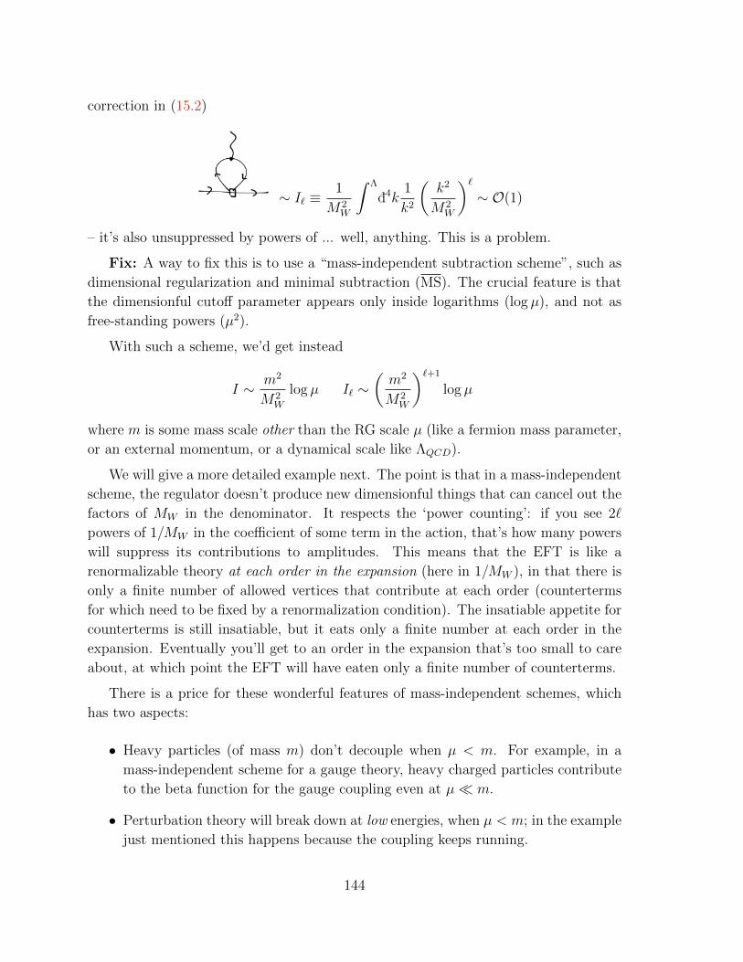
correction in (15.2)
∼ I` ≡1
M2W
∫ Λ
d4k1
k2
(k2
M2W
)`∼ O(1)
– it’s also unsuppressed by powers of ... well, anything. This is a problem.
Fix: A way to fix this is to use a “mass-independent subtraction scheme”, such as
dimensional regularization and minimal subtraction (MS). The crucial feature is that
the dimensionful cutoff parameter appears only inside logarithms (log µ), and not as
free-standing powers (µ2).
With such a scheme, we’d get instead
I ∼ m2
M2W
log µ I` ∼(m2
M2W
)`+1
log µ
where m is some mass scale other than the RG scale µ (like a fermion mass parameter,
or an external momentum, or a dynamical scale like ΛQCD).
We will give a more detailed example next. The point is that in a mass-independent
scheme, the regulator doesn’t produce new dimensionful things that can cancel out the
factors of MW in the denominator. It respects the ‘power counting’: if you see 2`
powers of 1/MW in the coefficient of some term in the action, that’s how many powers
will suppress its contributions to amplitudes. This means that the EFT is like a
renormalizable theory at each order in the expansion (here in 1/MW ), in that there is
only a finite number of allowed vertices that contribute at each order (counterterms
for which need to be fixed by a renormalization condition). The insatiable appetite for
counterterms is still insatiable, but it eats only a finite number at each order in the
expansion. Eventually you’ll get to an order in the expansion that’s too small to care
about, at which point the EFT will have eaten only a finite number of counterterms.
There is a price for these wonderful features of mass-independent schemes, which
has two aspects:
• Heavy particles (of mass m) don’t decouple when µ < m. For example, in a
mass-independent scheme for a gauge theory, heavy charged particles contribute
to the beta function for the gauge coupling even at µ m.
• Perturbation theory will break down at low energies, when µ < m; in the example
just mentioned this happens because the coupling keeps running.
144
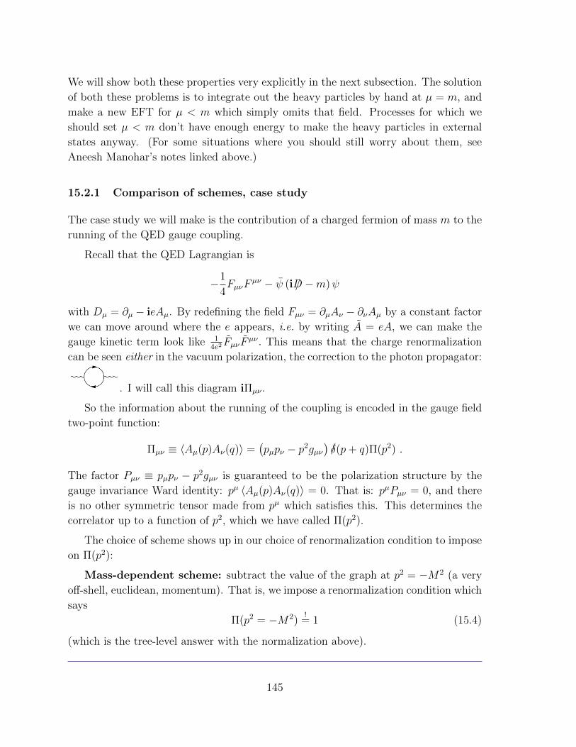
We will show both these properties very explicitly in the next subsection. The solution
of both these problems is to integrate out the heavy particles by hand at µ = m, and
make a new EFT for µ < m which simply omits that field. Processes for which we
should set µ < m don’t have enough energy to make the heavy particles in external
states anyway. (For some situations where you should still worry about them, see
Aneesh Manohar’s notes linked above.)
15.2.1 Comparison of schemes, case study
The case study we will make is the contribution of a charged fermion of mass m to the
running of the QED gauge coupling.
Recall that the QED Lagrangian is
−1
4FµνF
µν − ψ (i /D −m)ψ
with Dµ = ∂µ − ieAµ. By redefining the field Fµν = ∂µAν − ∂νAµ by a constant factor
we can move around where the e appears, i.e. by writing A = eA, we can make the
gauge kinetic term look like 14e2FµνF
µν . This means that the charge renormalization
can be seen either in the vacuum polarization, the correction to the photon propagator:
. I will call this diagram iΠµν .
So the information about the running of the coupling is encoded in the gauge field
two-point function:
Πµν ≡ 〈Aµ(p)Aν(q)〉 =(pµpν − p2gµν
)/δ(p+ q)Π(p2) .
The factor Pµν ≡ pµpν − p2gµν is guaranteed to be the polarization structure by the
gauge invariance Ward identity: pµ 〈Aµ(p)Aν(q)〉 = 0. That is: pµPµν = 0, and there
is no other symmetric tensor made from pµ which satisfies this. This determines the
correlator up to a function of p2, which we have called Π(p2).
The choice of scheme shows up in our choice of renormalization condition to impose
on Π(p2):
Mass-dependent scheme: subtract the value of the graph at p2 = −M2 (a very
off-shell, euclidean, momentum). That is, we impose a renormalization condition which
says
Π(p2 = −M2)!
= 1 (15.4)
(which is the tree-level answer with the normalization above).
145
The contribution of a fermion of massm and charge e is (factoring out the momentum-
conserving delta function):
p,µ p,ν = −∫
dDktr
((−ieγµ)
−i (/k +m)
k2 −m2(−ieγν)
−i(/p+ /k +m
)(p+ k)2 −m2
)The minus sign out front is from the fermion loop. Some boiling, which you can find
in Peskin (page 247) or Zee (§III.7), reduces this to something manageable. The steps
involved are: (1) a trick to combine the denominators, like the Feynman trick 1AB
=∫ 1
0dx(
1(1−x)A+xB
)2
. (2) some Dirac algebra, to turn the numerator into a polynomial
in k, p. As Zee says, our job in this course is not to train to be professional integrators.
The result of this boiling can be written
iΠµν = −e2
∫dD`
∫ 1
0
dxNµν
(`2 −∆)2
with ` = k+xp is a new integration variable, ∆ ≡ m2−x(1−x)p2, and the numerator
is
Nµν = 2`µ`ν − gµν`2 − 2x(1− x)pµpν + gµν(m2 + x(1− x)p2
)+ terms linear in `µ .
In dim reg, the one-loop vacuum polarization correction satisfies the gauge in-
varaince Ward identity Πµν = P µνδΠ2 (unlike the euclidean momentum cutoff which
is not gauge invariant). A peek at the tables of dim reg integrals shows that δΠ2 is:
δΠ2(p2)Peskin p. 252
= − 8e2
(4π)D/2
∫ 1
0
dxx(1− x)Γ(2−D/2)
∆2−D/2 µε
D→4= − e2
2π2
∫ 1
0
dxx(1− x)
(2
ε− log
(∆
µ2
))(15.5)
where we have introduced the heralded µ:
µ2 ≡ 4πµ2e−γE
where γE is the Euler-Mascheroni constant. In the second line of (15.5), we expanded
the Γ-function about D = 4; there are other singularities at other integer dimensions.
Mass-dependent scheme: Now back to our discussion of schemes. I remind you
that in a mass-independent scheme, we demand that the counterterm cancels δΠ2 when
we set the external momentum to p2 = −M2, so that the whole contribution at order
e2 is :
0(15.4)!
= Π(M)2 (p2 = −M2) = δ
(M)
F 2︸︷︷︸counterterm coefficient for 1
4FµνFµν
+δΠ2
146
=⇒ Π(M)2 (p2) =
e2
2π2
∫dxx(1− x) log
(m2 − x(1− x)p2
m2 + x(1− x)M2
).
Notice that the µs go away in this scheme.
Mass-Independent scheme: This is to be contrasted with what we get in a mass-
independent scheme, such as MS, in which Π is defined by the rule that we subtract
the 1/ε pole. This means that the counterterm is
δ(MS)
F 2 = − e2
2π2
2
ε
∫ 1
0
dxx(1− x)︸ ︷︷ ︸=1/6
.
(Confession: I don’t know how to state this in terms of a simple renormalization
condition on Π2. Also: the bar in MS refers to the (not so important) distinction
between µ and µ.) The resulting vacuum polarization function is
Π(MS)2 (p2) =
e2
2π2
∫ 1
0
dxx(1− x) log
(m2 − x(1− x)p2
µ2
).
Next we will talk about beta functions, and verify the claim above about the failure
of decoupling. First let me say some words about what is failing. What is failing – the
price we are paying for our power counting – is the basic principle of the RG, namely
that physics at low energies shouldn’t care about physics at high energies, except for
small corrections to couplings. An informal version of this statement is: you don’t need
to know about nuclear physics to make toast. A more formal version is the Appelquist-
Carazzone Decoupling Theorem, which I will not state (Phys. Rev. D11, 28565 (1975)).
So it’s something we must and will fix.
Beta functions. M : First in the mass-dependent scheme. Demanding that
physics is independent of our made-up RG scale, we find
0 = Md
dMΠ
(M)2 (p2) =
(M
∂
∂M+ β(M)
e e∂
∂e
)Π
(M)2 (p2) =
(M
∂
∂M+ β(M)
e ·2︸︷︷︸to this order
)Π
(M)2 (p2)
where I made the high-energy physics definition of the beta function35:
β(M)e ≡ 1
e(M∂Me) = −∂`e
e, M ≡ e−`M0 .
Here ` is the RG time again, it grows toward the IR. So we find
β(M)e = −1
2
(e2
2π
)∫ 1
0
dxx(1− x)
(−2M2x(1− x)
m2 +M2x(1− x)
)+O(e3)
35I’ve defined these beta functions to be dimensionless, i.e. they are ∂logM log(g); this convention
is not universally used.
147
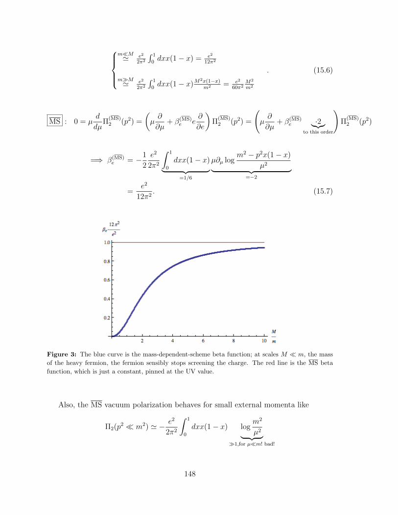
mM' e2
2π2
∫ 1
0dxx(1− x) = e2
12π2
mM' e2
2π2
∫ 1
0dxx(1− x)M
2x(1−x)m2 = e2
60π2M2
m2
. (15.6)
MS : 0 = µd
dµΠ
(MS)2 (p2) =
(µ∂
∂µ+ β(MS)
e e∂
∂e
)Π
(MS)2 (p2) =
(µ∂
∂µ+ β(MS)
e ·2︸︷︷︸to this order
)Π
(MS)2 (p2)
=⇒ β(MS)e = −1
2
e2
2π2
∫ 1
0
dxx(1− x)︸ ︷︷ ︸=1/6
µ∂µ logm2 − p2x(1− x)
µ2︸ ︷︷ ︸=−2
=e2
12π2. (15.7)
Figure 3: The blue curve is the mass-dependent-scheme beta function; at scales M m, the mass
of the heavy fermion, the fermion sensibly stops screening the charge. The red line is the MS beta
function, which is just a constant, pinned at the UV value.
Also, the MS vacuum polarization behaves for small external momenta like
Π2(p2 m2) ' − e2
2π2
∫ 1
0
dxx(1− x) logm2
µ2︸ ︷︷ ︸1,for µm! bad!
148
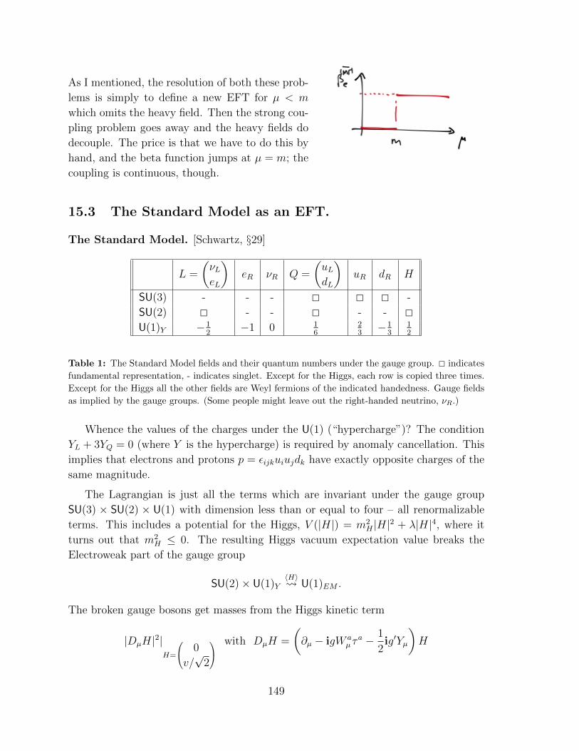
As I mentioned, the resolution of both these prob-
lems is simply to define a new EFT for µ < m
which omits the heavy field. Then the strong cou-
pling problem goes away and the heavy fields do
decouple. The price is that we have to do this by
hand, and the beta function jumps at µ = m; the
coupling is continuous, though.
15.3 The Standard Model as an EFT.
The Standard Model. [Schwartz, §29]
L =
(νLeL
)eR νR Q =
(uLdL
)uR dR H
SU(3) - - - 2 2 2 -
SU(2) 2 - - 2 - - 2U(1)Y −1
2−1 0 1
623−1
312
Table 1: The Standard Model fields and their quantum numbers under the gauge group. 2 indicates
fundamental representation, - indicates singlet. Except for the Higgs, each row is copied three times.
Except for the Higgs all the other fields are Weyl fermions of the indicated handedness. Gauge fields
as implied by the gauge groups. (Some people might leave out the right-handed neutrino, νR.)
Whence the values of the charges under the U(1) (“hypercharge”)? The condition
YL + 3YQ = 0 (where Y is the hypercharge) is required by anomaly cancellation. This
implies that electrons and protons p = εijkuiujdk have exactly opposite charges of the
same magnitude.
The Lagrangian is just all the terms which are invariant under the gauge group
SU(3) × SU(2) × U(1) with dimension less than or equal to four – all renormalizable
terms. This includes a potential for the Higgs, V (|H|) = m2H |H|2 + λ|H|4, where it
turns out that m2H ≤ 0. The resulting Higgs vacuum expectation value breaks the
Electroweak part of the gauge group
SU(2)× U(1)Y〈H〉 U(1)EM .
The broken gauge bosons get masses from the Higgs kinetic term
|DµH|2|H=
0
v/√
2
with DµH =
(∂µ − igW a
µ τa − 1
2ig′Yµ
)H
149
where Yµ is the hypercharge gauge boson, and W a, a = 1, 2, 3 are the SU(2) gauge
bosons. The photon and Z boson are(AµZµ
)=
(cos θw sin θw− sin θw cos θw
)(W 3µ
Yµ
).
There are also two massive W -bosons with electric charge ±1.
Fermion masses come from Yukawa couplings
LYukawa = −Y `ijLiHe
jR − Y
uij Q
iHdjR − YdijQ
i(iτ 2H?
)ujR + h.c.
The contortion with the τ 2 is required to make a hypercharge invariant. Plugging in
the Higgs vev to e.g. the lepton terms gives −meeLeR+h.c. with me = yev/√
2. There’s
lots of drama about the matrices Y which can mix the generations. the mass for the
νR (which maybe could not exist – it doesn’t have any charges at all) you’ll figure out
on the homework.
Here is a useful mnemonic for remembering the table of quantum numbers (possibly
it is more than that): There are larger simple Lie groups that contain the SM gauge
group as subgroups:
SU(3)× SU(2)× U(1)Y ⊂ SU(5) ⊂ SO(10)
one generation = 10⊕ 5⊕ 1 = 16
The singlet of SU(5) is the right-handed neutrino, but if we include it, one generation is
an irreducible (spinor) representation of SO(10). This idea is called grand unification.
It is easy to imagine that another instance of the Higgs mechanism accomplishes the
breaking down to the Standard Model. Notice that this means leptons and quarks are
in the same representations – they can turn into each other. This predicts that the
proton should not be perfectly stable. Next we’ll say more about this.
Beyond the Standard Model with EFT. At what energy does the Standard
Model stop working? Because of the annoying feature of renormalizibility, it doesn’t
tell us. However, we have experimental evidence against a cutoff on the Standard
Model (SM) at energies less than something like 10 TeV. The evidence I have in mind
is the absence of interactions of the form
δL =1
M2
(ψAψ
)·(ψBψ
)(where ψ represent various SM fermion fields and A,B can be various gamma and
flavor matrices) with M <∼ 10 TeV. Notice that I am talking now about interactions
other than the electroweak interactions, which as we’ve just discussed, for energies
150
above MW ∼ 80GeV cannot be treated as contact interactions – you can see the W s
propagate!
If such operators were present, we would have found different answers for exper-
iments at LEP. But such operators would be present if we consider new physics in
addition to the Standard Model (in most ways of doing it) at energies less than 10
TeV. For example, many interesting ways of coupling in new particles with masses
that make them accessible at the LHC would have generated such operators.
A little more explicitly: the Standard Model Lagrangian L0 contains all the renor-
malizable (i.e. engineering dimension ≤ 4) operators that you can make from its fields
(though the coefficients of the dimension 4 operators do vary through quite a large
range, and the coefficients of the two relevant operators – namely the identity operator
which has dimension zero, and the Higgs mass, which has engineering dimension two,
are strangely small, and so is the QCD θ angle).
To understand what lies beyond the Standard Model, we can use our knowledge
that whatever it is, it is probably heavy (it could also just be very weakly coupled,
which is a different story), with some intrinsic scale Λnew, so we can integrate it out
and include its effects by corrections to the Standard Model:
L = L0 +1
Λnew
O(5) +1
Λ2new
∑i
ciO(6)i
where the Os are made of SM fields, and have the indicated engineering dimensions,
and preserve the necessary symmetries of the SM.
In fact there is only one kind of operator of dimension 5:
O(5) = c5εij(Lc)iHjεklL
kH l
where H i = (h+, h0)i is the SU(2)EW Higgs doublet and Li = (νL, eL)i is an SU(2)EWdoublet of left-handed leptons, and Lc ≡ LTC where C is the charge conjugation
matrix. (I say ‘kind of operator’ because we can have various flavor matrices in here.)
On the problem set you get to see from whence such an operator might arise, and what
it does if you plug in the higgs vev 〈H〉 = (0, v). This term violates lepton number.
At dimension 6, there are operators that directly violate baryon number, such as
εαβγ(uR)cα(uR)β (uR)cγ eR.
You should read the above tangle of symbols as ‘qqq`’ – it turns three quarks into a
lepton. The epsilon tensor makes a color SU(3) singlet; this thing has the quantum
numbers of a baryon. The long lifetime of the proton (you can feel it in your bones –
see Zee p. 413) then directly constrains the scale of new physics appearing in front of
this operator.
151
Two more comments about this:
• If we didn’t know about the Standard Model, (but after we knew about QM and
GR and EFT (the last of which people didn’t know before the SM for some rea-
son)) we should have made the estimate that dimension-5 Planck-scale-suppressed
operators like 1MPlanck
pO would cause proton decay (into whatever O makes). This
predicts Γp ∼m3p
M2Planck
∼ 10−13s−1 which is not consistent with our bodies not glow-
ing. Actually it is a remarkable fact that there are no gauge-invariant operators
made of SM fields of dimension less than 6 that violate baryon number. This is
an emergent symmetry, expected to be violated by the UV completion.
• Surely nothing can prevent ∆L ∼(
1MPlanck
)2
qqq`. Happily, this is consistent
with the observed proton lifetime.
There are ∼ 102 dimension 6 operators that preserve baryon number, and therefore
are not as tightly constrained36 (Those that induce flavor-changing processes in the
SM are more highly constrained and must have Λnew > 104 TeV.) Two such operators
are considered equivalent if they differ by something which vanishes by the tree-level
SM equations of motion. This is the right thing to do, even for off-shell calculations
(like green’s functions and for fields running in loops). You know this from a previous
problem set: the EOM are true as operator equations – Ward identities resulting from
being free to change integration variables in the path integral37.
15.4 Pions
[Schwartz §28.1] Below the scale of electroweak symmetry breaking, we can forget the
W and Z bosons. Besides the 4-Fermi interactions, the remaining drama is QCD and
electromagnetism:
LQCD2 = −1
4F 2µν + i
∑α=L,R
∑f
qαf /Dqαf −mqMq.
Here f is a sum over quark flavors, which includes the electroweak doublets, u and
d. Let’s focus on just these two lightest flavors, u and d. We can diagonalize the
36Recently, humans have gotten better at counting these operators. See this paper.37 There are a few meaningful subtleties here, as you might expect if you recall that the Ward
identity is only true up to contact terms. The measure in the path integral can produce a Jacobian
which renormalizes some of the couplings; the changes in source terms will drop out of S-matrix
elements (recall our discussion of changing field variables in the Consequences of Unitarity section.)
but can change the form of Green’s functions. For more information on the use of eom to eliminate
redundant operators in EFT, see Arzt, hep-ph/9304230 and Georgi, “On-Shell EFT”.
152
mass matrix by a field redefinition (this is what makes the CKM matrix meaningful):
M =
(mu 0
0 md
). If it were the case that mu = md, we would have isospin symmetry
(u
d
)→ U
(u
d
), U ∈ SU(Nf = 2).
If, further, there were no masses m = 0, then L and R decouple and we also have chiral
symmetry, q → eiγ5αq, i.e.
qL → V qL, qR → V −1qR, V ∈ SU(Nf = 2).
Why do I restrict to SU(2) and not U(2)? The central bit of the axial symmetry
U(1)A is anomalous – it’s divergence is proportional to the gluon F ∧ F , which has all
kinds of nonzero matrix elements. It’s not a symmetry (see Peskin page 673 for more
detail). The central bit of the vectorlike transformation q → eiαq is baryon number, B.
(Actually this is anomalous under the full electroweak symmetry, but B − L is not).
The vacuum of QCD is mysterious, because of infrared slavery. Apparently it is the
case that
〈qfqf〉 = V 3
independent of flavor f . This condensate breaks
SU(2)L × SU(2)R → SU(2)isospin, (15.8)
the diagonal combination.
(u
d
)is a doublet. Since p = uαuβdγεαβγ, n = uαdβdγεαβγ,
this means that
(p
n
)is also a doublet. This symmetry is weakly broken by the dif-
ference of the masses md = 4.7MeV 6= mu = 2.15MeV and by the electromagnetic
interactions, since qd = −1/3 6= qu = 2/3.
This symmetry-breaking structure enormously constrains the dynamics of the color
singlets which are the low-energy excitations above the QCD vacuum (hadrons). Let
us use the EFT strategy. We know that the degrees of freedom must include (pseudo-
)Goldstone bosons for the symmetry breaking (15.8) (‘pseudo’ because of the weak
explicit breaking).
Effective field theory. Since QCD is strongly coupled in this regime, let’s use
the knowing-the-answer trick: the low energy theory must include some fields which
represent the breaking of the symmetry (15.8). One way to do this is to introduce a
field Σ which transforms like
SU(2)L × SU(2)R : Σ→ gLΣg†R, Σ† → gRΣ†g†L
153
(this will be called a linear sigma model, because Σ transforms linearly) and we can
make singlets (hence an action) out of |Σ|2 = ΣijΣ†ji = trΣΣ†:
L = |∂µΣ|2 +m2|Σ|2 − λ
4|Σ|4 + · · · (15.9)
which is designed to have a minimum at 〈Σ〉 = V√2
(1 0
0 1
), with V = 2m/
√λ, which
preserves SU(2)isospin. We can parametrize the fluctuations about this configuration as
Σ(x) =V + σ(x)√
2e
2iπa(x)τa
Fπ
where Fπ will be chosen to give πa(x) canonical kinetic terms. Under gL/R = eiθL/Rτa,
the pion field transforms as
πa → πa +Fπ2
(θaL − θaR)︸ ︷︷ ︸nonlinear realization of SU(2)axial
− 1
2fabc (θaL + θaR) πc︸ ︷︷ ︸
linear realiz’n (adj rep) of SU(2)isospin
.
The fields π±, π0 create pions, they transform in the adjoint representation of the
diagonal SU(2)isospin, and they shift under the broken symmetry. This shift symmetry
forbids mass terms π2. The radial excitation σ, on the other hand, is a fiction which
we’ve introduced in (15.9), and which has no excuse to stick around at low energies
(and does not). We can put it out of its misery by taking m → ∞, λ → ∞ fixing Fπ.
In the limit, the useful field to use is
U(x) ≡√
2
VΣ(x)|σ=0 = e
2iπaτa
Fπ
which is unitary UU † = U †U = 1. This last identity means that all terms in an action
for U require derivatives, so (again) no mass for π. The most general Lagrangian for
U can be written as an expansion in derivatives, and is called the chiral Lagrangian:
Lχ =F 2π
4trDµUD
µU †+L1tr(DµUD
µU †)2
+L2trDµUDνU†trDνU †DµU+L3trDµUD
µU †DνUDνU †+· · ·
(15.10)
In terms of π, the leading terms are
Lχ =1
2∂µπ
a∂µπa+1
F 2π
(−1
3π0π0Dµπ
+Dµπ− + · · ·)
+1
F 4π
(1
18
(π−π+
)2Dµπ
0Dµπ0 + · · ·)
This fixes the relative coefficients of many irrelevant interactions, all with two deriva-
tives, suppressed by powers of Fπ. The expansion of the Li terms have four derivatives,
and are therefore suppressed by further powers of E/Fπ.
154
Pion masses. The pions aren’t actually massless: mπ± ∼ 140MeV. In terms of
quarks, one source for such a thing is the quark mass term L 3 qMq. This breaks the
isospin symmetry if the eigenvalues of M aren’t equal. But an invariance of L is
qL/R → gL/RqL/R, M → gLMg†R. (15.11)
Think of M as a background field (such a thing is sometimes called a spurion). If M
were an actual dynamical field, then (15.11) would be a symmetry. In the effective
action which summarizes all the drama of strong-coupling QCD in terms of pions, the
field M should still be there, and if we transform it as in (15.11), it should still be an
invariance. Maybe we’re going to do the path integral over M later. (This is the same
strategy we used when deriving the vertical-tangents condition in the Bose-Hubbard
phase diagram.)
So the chiral lagrangian Lχ should depend on M and (15.11) should be an invari-
ance. This determines
∆Lχ =V 3
2tr(MU +M †U †
)+ · · · = V 3(mu +md)−
V 3
2F 2π
(mu +md)∑a
π2a +O(π2).
The coefficient V 3 is chosen so that the first term matches 〈qMq〉 = V 3(mu+md). The
second term then gives
m2π '
V 3
F 2π
(mu +md)
which is called the Gell-Mann Oakes Renner relation.
Electroweak interactions. You may have noticed that I used covariant-looking
Ds in (15.10). That’s because the SU(2)L symmetry we’ve been speaking about is
actually gauged by W aµ . (The electroweak gauge boson kinetic terms are in the · · · of
(15.10).) Recall that
LWeak 3g
2W aµ
Jaµ − J5aµ︸ ︷︷ ︸
‘V’ - ‘A’
= W aµ
(VijQiγ
µ(1− γ5)τaQj + Liγµτa(1− γ5)Li
)
where Q1 =
(u
d
), L1 =
(e
νe
)are doublets of SU(2)L.
Now, in equations, the statement “a pion is a Goldstone boson for the axial SU(2)”
is:
〈0| J5aµ (x)
∣∣πb(p)⟩ = ipµFπe−ip·xδab.
If the vacuum were invariant under the symmetry transformation generated by Jµ, the
BHS would vanish. The momentum dependence implements the fact that a global
155
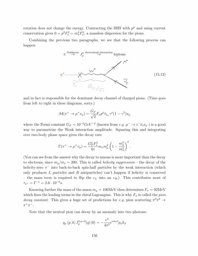
rotation does not change the energy. Contracting the BHS with pµ and using current
conservation gives 0 = p2F 2π = m2
πF2π , a massless dispersion for the pions.
Combining the previous two paragraphs, we see that the following process can
happen
πGoldstone→ J5
µelectroweak interaction→ leptons
(15.12)
and in fact is responsible for the dominant decay channel of charged pions. (Time goes
from left to right in these diagrams, sorry.)
M(π+ → µ+νµ) =GF√
2Fπp
µvνµγµ(1− γ5)uµ
where the Fermi constant GF ∼ 10−5GeV −2 (known from e.g. µ− → e−νeνµ ) is a good
way to parametrize the Weak interaction amplitude. Squaring this and integrating
over two-body phase space gives the decay rate
Γ(π+ → µ+νµ) =G2FF
2π
4πmπm
2µ
(1−
m2µ
m2π
)2
.
(You can see from the answer why the decay to muons is more important than the decay
to electrons, since mµ/me ∼ 200. This is called helicity suppression – the decay of the
helicity-zero π− into back-to-back spin-half particles by the weak interaction (which
only produces L particles and R antiparticles) can’t happen if helicity is conserved
– the mass term is required to flip the eL into an eR.) This contributes most of
τπ+ = Γ−1 = 2.6 · 10−8s.
Knowing further the mass of the muon mµ = 106MeV then determines Fπ = 92MeV
which fixes the leading terms in the chiral Lagrangian. This is why Fπ is called the pion
decay constant. This gives a huge set of predictions for e.g. pion scattering π0π0 →π+π−.
Note that the neutral pion can decay by an anomaly into two photons:
qµ 〈p, k| J5,a=3µ (q) |0〉 = − e2
4π2ενλαβpαkβ
156
where 〈p, k| is a state with two photons, and this is a matrix element of the JeJeJisospin
anomaly,
∂µJµ5a = − e2
16π2ενλαβFνλFαβtr
(τaQ2
)where Q =
(2/3 0
0 −1/3
)is the quark charge matrix.
SU(3) and baryons. The strange quark mass is also pretty small ms ∼ 95MeV,
and 〈ss〉 ∼ V 3. This means the approximate invariance and symmetry breaking pattern
is actually SU(3)L × SU(3)R → SU(3)diag, meaning that there are 16 − 8 = 8 pseudo
NGBs. Besides π±,0, the others are the kaons K±,0 and η. It’s still only the SU(2)Lthat’s gauged.
We can also include baryons B = εαβγqαqβqγ. Since q ∈ 3 of SU(3), the baryons are
in the representation
3⊗ 3⊗ 3 = (6⊕ 3)⊗ 3 = 10⊕ 8⊕ 8⊕ 1
⊗ ⊗ = ( ⊕ )⊗ = ⊕ ⊕ ⊕ (15.13)
The proton and neutron are in one of the octets. This point of view brought some
order (and some predictions) to the otherwise-bewildering zoo of hadrons.
Returning to the two-flavor SU(2) approximation, We can include the nucleons
NL/R =
(p
n
)L/R
and couple them to pions by the symmetric coupling
L 3 λNNπNLΣNR.
The expectation value for Σ gives a nucleon mass: mN = λNNπFπ. This is a cheap
version of the Goldberger-Treiman relation; for a better one see Peskin pp. 670-672.
WZW terms in the chiral Lagrangian. Finally, I would be remiss not to
mention that the chiral Lagrangian must be supplemented by WZW terms to have the
right realization of symmetries (in order to encode all the effects of anomalies, and in
order to violate π → −π which is not a symmetry of QCD). This is where those terms
were first discovered, and where it was realized that their coefficients are quantized.
In particular the coefficient of the WZW term W4[U ] here is Nc, the number of colors,
as Witten shows by explicitly coupling to electromagnetism, and finding the term that
encodes π0 → γγ. One dramatic consequence here is that the chiral Lagrangian (with
some higher-derivative terms) has a topological soliton solution (the skyrmion) which is
a fermion if the number of colors of QCD is odd. It is a fermion because the WZW term
evaluates to π on a spacetime trajectory where the soliton makes a 2π rotation. The
baryon number of this configuration comes from the anomalous (WZW) contribution
157
to the baryon number current Bµ =εµναβ24π2 trU−1∂νUU
−1∂αUU−1∂βU whose conserved
charge∫
spaceB0 is the winding number of the map from space (plus the point at infinity)
to the space of goldstones S3 → SU(3)× SU(3)/SU(3)preserved ' SU(3)broken.
[End of Lecture 61]
15.5 Quantum Rayleigh scattering
We didn’t have lecture time for the remaining sections, but you might still enjoy them.
[from hep-ph/9606222 and nucl-th/0510023] Why is the sky blue? Basically, it’s
because the blue light from the sun scatters in the atmosphere more than the red light,
and you (I hope) only look at the scattered light.
Here is an understanding of this fact using the EFT logic. Consider the scattering
of photons off atoms at low energies. Low energy means that the photon does not have
enough energy to probe the substructure of the atom – it can’t excite the electrons or
the nuclei. This means that the atom is just a particle, with some mass M .
The dofs are just the photon field and the field that creates an atom.
The symmetries are Lorentz invariance and charge conjugation invariance and par-
ity. We’ll use the usual redundant description of the photon which has also gauge
invariance.
The cutoff is the energy ∆E that it takes to excite atomic energy levels we’ve left
out of the discussion. We allow no inelastic scattering. This means we require
Eγ ∆E ∼ α
a0
a−10 Matom
Because of this separation of scales, we can also ignore the recoil of the atom, and treat
it as infinitely heavy.
Since there are no charged objects in sight – atoms are neutral – gauge invariance
means the Lagrangian can depend on the field strength Fµν . Let’s call the field which
destroys an atom with velocity v φv. vµvµ = 1 and vµ = (1, 0, 0, 0)µ in the atom’s rest
frame. The Lagrangian can depend on vµ. We can write a Lagrangian for the free
atoms as
Latom = φ†vivµ∂µφv .
This action is related by a boost to the statement that the atom at rest has zero energy
– in the rest frame of the atom, the eom is just ∂tφv=(1,~0) = 0.
So the Lagrangian density is
LMaxwell[A] + Latom[φv] + Lint[A, φv]
158
and we must determine Lint. It is made from local, Hermitian, gauge-invariant, Lorentz
invariant operators we can construct out of φv, Fµν , vµ, ∂µ (It can only depend on Fµν =
∂µAν−∂νAµ, and not Aµ directly, by gauge invariance.). It should actually only depend
on the combination φ†vφv since we will not create and destroy atoms. Therefore
Lint = c1φ†vφvFµνF
µν + c2φ†vφvv
σFσµvλFλµ + c3φ
†vφv(vλ∂λ
)FµνF
µν + . . .
. . . indicates terms with more derivatives and more powers of velocity (i.e. an expansion
in ∂ · v). Which are the most important terms at low energies? Demanding that the
Maxwell term dominate, we get the power counting rules (so time and space should
scale the same way):
[∂µ] = 1, [Fµν ] = 2
This then implies [φv] = 3/2, [v] = 0 and therefore
[c1] = [c2] = −3, [c3] = −4 .
Terms with more partials are more irrelevant.
What makes up these dimensions? They must come from the length scales that we
have integrated out to get this description – the size of the atom a0 ∼ αme and the
energy gap between the ground state and the electronic excited states ∆E ∼ α2me.
For Eγ ∆E, a−10 , we can just keep the two leading terms.
In the rest frame of the atom, these two leading terms c1,2 represent just the scat-
tering of E and B respectively. To determine their coefficients one would have to do
a matching calculation to a more complete theory (compute transition rates in a the-
ory that does include extra energy levels of the atom). But a reasonable guess is just
that the scale of new physics (in this case atomic physics) makes up the dimensions:
c1 ' c2 ' a30. (In fact the magnetic term c2 comes with extra factor of v/c which
suppresses it.) The scattering cross section then goes like σ ∼ c2i ∼ a6
0; dimensional
analysis ([σ] = −2 is an area, [a60] = −6) then tells us that we have to make up four
powers with the only other scale around:
σ ∝ E4γa
60.
(The factor of E2γ in the amplitude arises from ~E ∝ ∂t ~A.) Blue light, which has about
twice the energy of red light, is therefore scattered 16 times as much.
The leading term that we left out is the one with coefficient c3. The size of this
coefficient determines when our approximations break down. We might expect this to
come from the next smallest of our neglected scales, namely ∆E. That is, we expect
σ ∝ E4γa
60
(1 +O
(Eγ∆E
)).
The ratio in the correction terms is appreciable for UV light.
159
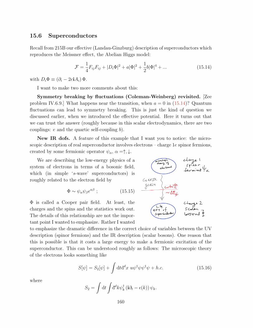
15.6 Superconductors
Recall from 215B our effective (Landau-Ginzburg) description of superconductors which
reproduces the Meissner effect, the Abelian Higgs model:
F =1
4FijFij + |DiΦ|2 + a|Φ|2 +
1
2b|Φ|4 + ... (15.14)
with DiΦ ≡ (∂i − 2eiAi) Φ.
I want to make two more comments about this:
Symmetry breaking by fluctuations (Coleman-Weinberg) revisited. [Zee
problem IV.6.9.] What happens near the transition, when a = 0 in (15.14)? Quantum
fluctuations can lead to symmetry breaking. This is just the kind of question we
discussed earlier, when we introduced the effective potential. Here it turns out that
we can trust the answer (roughly because in this scalar electrodynamics, there are two
couplings: e and the quartic self-coupling b).
New IR dofs. A feature of this example that I want you to notice: the micro-
scopic description of real superconductor involves electrons – charge 1e spinor fermions,
created by some fermionic operator ψα, α =↑, ↓.
We are describing the low-energy physics of a
system of electrons in terms of a bosonic field,
which (in simple ‘s-wave’ superconductors) is
roughly related to the electron field by
Φ ∼ ψαψβεαβ ; (15.15)
Φ is called a Cooper pair field. At least, the
charges and the spins and the statistics work out.
The details of this relationship are not the impor-
tant point I wanted to emphasize. Rather I wanted
to emphasize the dramatic difference in the correct choice of variables between the UV
description (spinor fermions) and the IR description (scalar bosons). One reason that
this is possible is that it costs a large energy to make a fermionic excitation of the
superconductor. This can be understood roughly as follows: The microscopic theory
of the electrons looks something like
S[ψ] = S2[ψ] +
∫dtddx uψ†ψψ†ψ + h.c. (15.16)
where
S2 =
∫dt
∫ddkψ†k (i∂t − ε(k))ψk.
160
Notice the strong similarity with the XY model action in our discussion of the RG (in
fact this similarity was Shankar’s motivation for explaining the RG for the XY model in
the (classic) paper I cited there). A mean field theory description of the condensation of
Cooper pairs (15.15) is obtained by replacing the quartic term in (15.16) by expectation
values:
SMFT [ψ] = S2[ψ] +
∫dtddx u 〈ψψ〉ψ†ψ† + h.c.
= S2[ψ] +
∫dtddx uΦψ†ψ† + h.c. (15.17)
So an expectation value for Φ is a mass for the fermions. It is a funny kind of symmetry-
breaking mass, but if you diagonalize the quadratic operator in (15.17) (actually it is
done below) you will find that it costs an energy of order ∆Eψ = u 〈Φ〉 to excite a
fermion. That’s the cutoff on the LG EFT.
A general lesson from this example is: the useful degrees of freedom at low energies
can be very different from the microscopic dofs.
15.6.1 Lightning discussion of BCS.
I am sure that some of you are nervous about the step from S[ψ] to SMFT [ψ] above. To
make ourselves feel better about it, I will say a few more words about the steps from
the microscopic model of electrons (15.16) to the LG theory of Cooper pairs (these
steps were taken by Bardeen, Cooper and Schreiffer (BCS)).
First recall the Hubbard-Stratonovich transformation aka completing the square. in
0+0 dimensional field theory:
e−iux4
=√
2πu
∫ ∞−∞
dσ e−1iuσ2−2ix2σ . (15.18)
At the cost of introducing an extra field σ, we turn a quartic term in x into a quadratic
term in x. The RHS of (15.18) is gaussian in x and we know how to integrate it over
x. (The version with i is relevant for the real-time integral.) Notice the weird extra
factor of i lurking in (15.18). This can be understood as arising because we are trying
to use a scalar field σ, to mediate a repulsive interaction (which it is, for positive u)
(see Zee p. 193, 2nd Ed).
Actually, we’ll need a complex H-S field:
e−iux2x2
= 2πu2
∫ ∞−∞
dσ
∫ ∞−∞
dσ e−1iu|σ|2−ix2σ−ix2σ . (15.19)
(The field-independent prefactor is, as usual, not important for path integrals.)
161
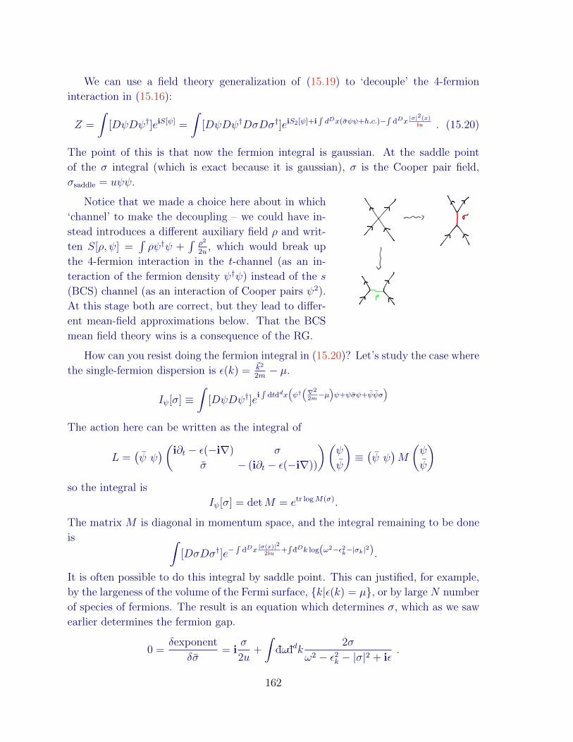
We can use a field theory generalization of (15.19) to ‘decouple’ the 4-fermion
interaction in (15.16):
Z =
∫[DψDψ†]eiS[ψ] =
∫[DψDψ†DσDσ†]eiS2[ψ]+i
∫dDx(σψψ+h.c.)−
∫dDx
|σ|2(x)iu . (15.20)
The point of this is that now the fermion integral is gaussian. At the saddle point
of the σ integral (which is exact because it is gaussian), σ is the Cooper pair field,
σsaddle = uψψ.
Notice that we made a choice here about in which
‘channel’ to make the decoupling – we could have in-
stead introduces a different auxiliary field ρ and writ-
ten S[ρ, ψ] =∫ρψ†ψ +
∫ρ2
2u, which would break up
the 4-fermion interaction in the t-channel (as an in-
teraction of the fermion density ψ†ψ) instead of the s
(BCS) channel (as an interaction of Cooper pairs ψ2).
At this stage both are correct, but they lead to differ-
ent mean-field approximations below. That the BCS
mean field theory wins is a consequence of the RG.
How can you resist doing the fermion integral in (15.20)? Let’s study the case where
the single-fermion dispersion is ε(k) =~k2
2m− µ.
Iψ[σ] ≡∫
[DψDψ†]ei∫
dtddx(ψ†(∇2
2m−µ)ψ+ψσψ+ψψσ
)
The action here can be written as the integral of
L =(ψ ψ
)(i∂t − ε(−i∇) σ
σ − (i∂t − ε(−i∇))
)(ψ
ψ
)≡(ψ ψ
)M
(ψ
ψ
)so the integral is
Iψ[σ] = detM = etr logM(σ).
The matrix M is diagonal in momentum space, and the integral remaining to be done
is ∫[DσDσ†]e−
∫dDx
|σ(x)|22iu
+∫
dDk log(ω2−ε2k−|σk|2).
It is often possible to do this integral by saddle point. This can justified, for example,
by the largeness of the volume of the Fermi surface, k|ε(k) = µ, or by large N number
of species of fermions. The result is an equation which determines σ, which as we saw
earlier determines the fermion gap.
0 =δexponent
δσ= i
σ
2u+
∫dωddk
2σ
ω2 − ε2k − |σ|2 + iε.
162

We can do the frequency integral by residues:∫dω
1
ω2 − ε2k − |σ|2 + iε=
1
2π2πi
1
2√ε2k + |σ|2
.
The resulting equation is naturally called the gap equation:
1 = −2u
∫ddp′
1√ε(p′)2 + |σ|2
(15.21)
which you can imagine solving self-consistently for σ. Plugging back into the action
(15.20) says that σ determines the energy cost to have electrons around; more precisely,
σ is the energy required to break a Cooper pair.
Comments:
• If we hadn’t restricted to a delta-function 4-fermion interaction u(p, p′) = u0 at
the outset, we would have found a more general equation like
σ(~p) = −1
2
∫ddp′
u(p, p′)σ(~p′)√ε(p′)2 + |σ(p′)|2
.
• Notice that a solution of (15.21) requires u < 0, an attractive interaction. Super-
conductivity happens because the u that appears here is not the bare interaction
between electrons, which is certainly repulsive (and long-ranged). This is where
the phonons come in in the BCS discussion.
• I haven’t included here effects of the fluctuations of the fermions. In fact, they
make the four-fermion interaction which leads to Cooper pairing marginally rel-
evant. This breaks the degeneracy in deciding how to split up the ψψψ†ψ† into
e.g. ψψσ or ψ†ψρ. BCS wins. This is explained beautifully in Polchinski, lecture
2, and R. Shankar. If there were time, I would summarize the EFT framework
for understanding this in §15.7.
• A conservative perspective on the preceding calculation is that we have made a
variational ansatz for the groundstate wavefunction, and the equation we solve
for σ is minimizing the variational energy – finding the best wavefunction within
the ansatz.
• I’ve tried to give the most efficient introduction I could here. I left out any
possibility of k-dependence or spin dependence of the interactions or the pair
field, and I’ve conflated the pair field with the gap. In particular, I’ve been
sloppy about the dependence on k of σ above.
163
• You studied very closely related manipulation on a previous problem set, in an
example (the Gross-Neveu model) where the saddle point is justified by large N .
15.7 Effective field theory of Fermi surfaces
[Polchinski, lecture 2, and R. Shankar] Electrically conducting solids are a remarkable
phenomenon. An arbitrarily small electric field ~E leads to a nonzero current ~j = σ ~E.
This means that there must be gapless modes with energies much less than the natural
cutoff scale in the problem.
Scales involved: The Planck scale of solid state physics (made by the logic by
which Planck made his quantum gravity energy scale, namely by making a quantity
with dimensions of energy out of the available constants) is
E0 =1
2
e4m
~2=
1
2
e2
a0
∼ 13eV
(where m ≡ me is the electron mass and the factor of 2 is an abuse of outside informa-
tion) which is the energy scale of chemistry. Chemistry is to solids as the melting of
spacetime is to particle physics. There are other scales involved however. In particular
a solid involves a lattice of nuclei, each with M m (approximately the proton mass).
So m/M is a useful small parameter which controls the coupling between the electrons
and the lattice vibrations. Also, the actual speed of light c vF can generally also
be treated as ∞ to first approximation. vF/c suppresses spin orbit couplings (though
large atomic numbers enhance them: λSO ∝ ZvF/c).
Let us attempt to construct a Wilsonian-natural effective field theory of this phe-
nomenon. The answer is called Landau Fermi Liquid Theory. What are the right low-
energy degrees of freedom? Let’s make a guess that they are like electrons – fermions
with spin and electric charge. They will not have exactly the properties of free elec-
trons, since they must incorporate the effects of interactions with all their friends. The
‘dressed’ electrons are called quasielectrons, or more generally quasiparticles.
Given the strong interactions between so many particles, why should the dofs have
anything at all to do with electrons? Landau’s motivation for this description (which
is not always correct) is that we can imagine starting from the free theory and adia-
batically turning up the interactions. If we don’t encounter any phase transition along
the way, we can follow each state of the free theory, and use the same labels in the
interacting theory.
164
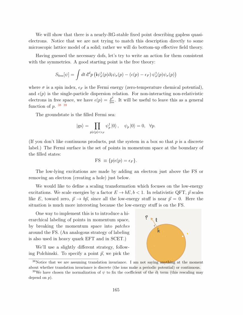
We will show that there is a nearly-RG-stable fixed point describing gapless quasi-
electrons. Notice that we are not trying to match this description directly to some
microscopic lattice model of a solid; rather we will do bottom-up effective field theory.
Having guessed the necessary dofs, let’s try to write an action for them consistent
with the symmetries. A good starting point is the free theory:
Sfree[ψ] =
∫dt ddp
(iψ†σ(p)∂tψσ(p)− (ε(p)− εF )ψ†σ(p)ψσ(p)
)where σ is a spin index, εF is the Fermi energy (zero-temperature chemical potential),
and ε(p) is the single-particle dispersion relation. For non-interacting non-relativistic
electrons in free space, we have ε(p) = p2
2m. It will be useful to leave this as a general
function of p. 38 39
The groundstate is the filled Fermi sea:
|gs〉 =∏
p|ε(p)<εF
ψ†p |0〉 , ψp |0〉 = 0, ∀p.
(If you don’t like continuous products, put the system in a box so that p is a discrete
label.) The Fermi surface is the set of points in momentum space at the boundary of
the filled states:
FS ≡ p|ε(p) = εF.
The low-lying excitations are made by adding an electron just above the FS or
removing an electron (creating a hole) just below.
We would like to define a scaling transformation which focuses on the low-energy
excitations. We scale energies by a factor E → bE, b < 1. In relativistic QFT, ~p scales
like E, toward zero, ~p → b~p, since all the low-energy stuff is near ~p = 0. Here the
situation is much more interesting because the low-energy stuff is on the FS.
One way to implement this is to introduce a hi-
erarchical labeling of points in momentum space,
by breaking the momentum space into patches
around the FS. (An analogous strategy of labeling
is also used in heavy quark EFT and in SCET.)
We’ll use a slightly different strategy, follow-
ing Polchinski. To specify a point ~p, we pick the
38Notice that we are assuming translation invariance. I am not saying anything at the moment
about whether translation invariance is discrete (the ions make a periodic potential) or continuous.39We have chosen the normalization of ψ to fix the coefficient of the ∂t term (this rescaling may
depend on p).
165
nearest point ~k on the FS, ε(~k) = εF (draw a line
perpendicular to the FS from ~p), and let
~p = ~k + ~.
So d− 1 of the components are determined by ~k and one is determined by `. (Clearly
there are some exceptional cases if the FS gets too wiggly. Ignore these for now.)
ε(p)− εF = `vF (~k) +O(`2), vF ≡ ∂pε|p=k.
So a scaling rule which accomplishes our goal of focusing on the FS is
E → bE, ~k → ~k, ~l→ b~.
This implies
dt→ b−1dt, dd−1~k → dd−1~k, d~→ bd~, ∂t → b∂t
Sfree =
∫dt dd−1~k d~︸ ︷︷ ︸
∼b0
iψ†(p) ∂t︸︷︷︸∼b1
ψ(p)− `vF (k)︸ ︷︷ ︸∼b1
ψ†(p)ψ(p)
In order to make this go like b0 we require ψ → b−
12ψ near the free fixed point.
Next we will play the EFT game. To do so we must enumerate the symmetries we
demand of our EFT:
1. Particle number, ψ → eiθψ
2. Spatial symmetries: either (a) continuous translation invariance and rotation
invariance (as for e.g. liquid 3He) or (b) lattice symmetries. This means that
momentum space is periodically identified, roughly p ' p + 2π/a where a is the
lattice spacing (the set of independent momenta is called the Brillouin zone (BZ))
and p is only conserved modulo an inverse lattice vector 2π/a; the momentum
There can also be some remnant of rotation invariance preserved by the lattice.
Case (b) reduces to case (a) if the Fermi surface does not go near the edges of
the BZ.
3. Spin rotation symmetry, SU(n) if σ = 1..n. In the limit with c → ∞, this is an
internal symmetry, independent of rotations.
4. Let’s assume that ε(p) = ε(−p), which is a consequence of e.g. parity invariance.
Now we enumerate all terms analytic in ψ (since we are assuming that there are no
other low-energy operators integrating out which is the only way to get non-analytic
166

terms in ψ) and consistent with the symmetries; we can order them by the number of
fermion operators involved. Particle number symmetry means every ψ comes with a
ψ†. The possible quadratic terms are:∫dt dd−1~k d~︸ ︷︷ ︸
∼b0µ(k)ψ†σ(p)ψσ(p)︸ ︷︷ ︸
∼b−1
∼ b−1
is relevant. This is like a mass term. But don’t panic: it just shifts the FS around. The
existence of a Fermi surface is Wilson-natural; any precise location or shape (modulo
something enforced by symmetries, like roundness) is not.
Adding one extra ∂t or factor of ` costs a b1 and makes the operator marginal; those
terms are already present in Sfree. Adding more than one makes it irrelevant.
Quartic terms:
S4 =
∫dt
4∏i=1
dd−1~kid~i︸ ︷︷ ︸∼b−1+4−4/2
u(4 · · · 1)ψ†σ(p1)ψσ(p3)ψ†σ′(p2)ψσ′(p4)δd(~p1 + ~p2 − ~p3 − ~p4)
Note the similarity with the discussion of the XY model in §??. The minus signs on
p3,4 is because ψ(p) removes a particle with momentum p. We assume u depends only
on k, σ, so does not scale – this will give the most relevant piece. How does the delta
function scale?
δd (~p1 + ~p2 − ~p3 − ~p4) = δd (k1 + k2 − k3 − k4 + `1 + `2 − `3 − `4)?' δd (k1 + k2 − k3 − k4)
In the last (questioned) step, we used the fact that ` k to ignore the contributions
of the `s. If this is correct then the delta function does not scale (since ks do not),
and S4 ∼ b1 is irrelevant (and quartic interactions with derivatives are moreso). If this
were correct, the free-fixed point would be exactly stable.
There are two important subtleties: (1) there exist phonons. (2) the questioned
equality above is questionable because of kinematics of the Fermi surface. We will
address these two issues in reverse order.
The kinematic subtlety in the treatment of the
scaling of δ(p1 + p2 − p3 − p4) arises because of the
geometry of the Fermi surface. Consider scattering
between two points on the FS, where (in the labeling
convention above)
p3 = p1 + δk1 + δ`1, p4 = p2 + δk2 + δ`2,
167
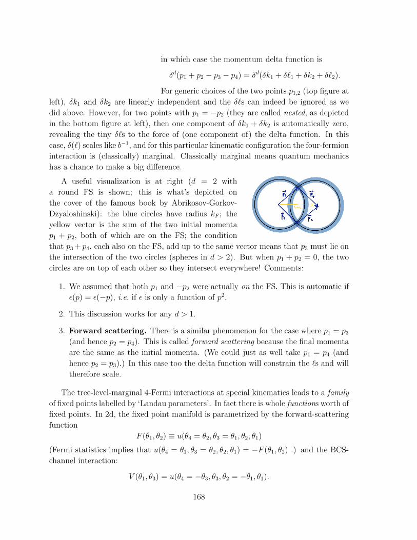
in which case the momentum delta function is
δd(p1 + p2 − p3 − p4) = δd(δk1 + δ`1 + δk2 + δ`2).
For generic choices of the two points p1,2 (top figure at
left), δk1 and δk2 are linearly independent and the δ`s can indeed be ignored as we
did above. However, for two points with p1 = −p2 (they are called nested, as depicted
in the bottom figure at left), then one component of δk1 + δk2 is automatically zero,
revealing the tiny δ`s to the force of (one component of) the delta function. In this
case, δ(`) scales like b−1, and for this particular kinematic configuration the four-fermion
interaction is (classically) marginal. Classically marginal means quantum mechanics
has a chance to make a big difference.
A useful visualization is at right (d = 2 with
a round FS is shown; this is what’s depicted on
the cover of the famous book by Abrikosov-Gorkov-
Dzyaloshinski): the blue circles have radius kF ; the
yellow vector is the sum of the two initial momenta
p1 + p2, both of which are on the FS; the condition
that p3 + p4, each also on the FS, add up to the same vector means that p3 must lie on
the intersection of the two circles (spheres in d > 2). But when p1 + p2 = 0, the two
circles are on top of each other so they intersect everywhere! Comments:
1. We assumed that both p1 and −p2 were actually on the FS. This is automatic if
ε(p) = ε(−p), i.e. if ε is only a function of p2.
2. This discussion works for any d > 1.
3. Forward scattering. There is a similar phenomenon for the case where p1 = p3
(and hence p2 = p4). This is called forward scattering because the final momenta
are the same as the initial momenta. (We could just as well take p1 = p4 (and
hence p2 = p3).) In this case too the delta function will constrain the `s and will
therefore scale.
The tree-level-marginal 4-Fermi interactions at special kinematics leads to a family
of fixed points labelled by ‘Landau parameters’. In fact there is whole functions worth of
fixed points. In 2d, the fixed point manifold is parametrized by the forward-scattering
function
F (θ1, θ2) ≡ u(θ4 = θ2, θ3 = θ1, θ2, θ1)
(Fermi statistics implies that u(θ4 = θ1, θ3 = θ2, θ2, θ1) = −F (θ1, θ2) .) and the BCS-
channel interaction:
V (θ1, θ3) = u(θ4 = −θ3, θ3, θ2 = −θ1, θ1).
168
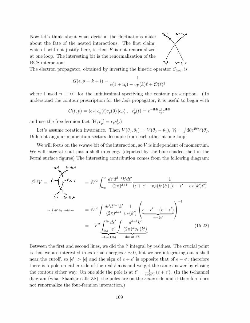
Now let’s think about what decision the fluctuations make
about the fate of the nested interactions. The first claim,
which I will not justify here, is that F is not renormalized
at one loop. The interesting bit is the renormalization of the
BCS interaction:
The electron propagator, obtained by inverting the kinetic operator Sfree, is
G(ε, p = k + l) =1
ε(1 + iη)− vF (k)`+O(`)2
where I used η ≡ 0+ for the infinitesimal specifying the contour prescription. (To
understand the contour prescription for the hole propagator, it is useful to begin with
G(t, p) = 〈εF | c†p(t)cp(0) |εF 〉 , c†p(t) ≡ e−iHtc†peiHt
and use the free-fermion fact [H, c†p] = εpc†p.)
Let’s assume rotation invariance. Then V (θ3, θ1) = V (θ3 − θ1), Vl =∫
dθeilθV (θ).
Different angular momentum sectors decouple from each other at one loop.
We will focus on the s-wave bit of the interaction, so V is independent of momentum.
We will integrate out just a shell in energy (depicted by the blue shaded shell in the
Fermi surface figures) The interesting contribution comes from the following diagram:
δ(1)V = = iV 2
∫ ε0
bε0
dε′dd−1k′d`′
(2π)d+1
1
(ε+ ε′ − vF (k′)`′) (ε− ε′ − vF (k′)`′)
do
∫d`′
by residues = iV 2
∫dε′dd−1k′
(2π)d+1
1
vF (k′)
ε− ε′ − (ε+ ε′)︸ ︷︷ ︸=−2ε′
−1
= −V 2
∫ ε0
bε0
dε′
ε′︸ ︷︷ ︸=log(1/b)
∫dd−1k′
(2π)dvF (k′)︸ ︷︷ ︸dos at FS
(15.22)
Between the first and second lines, we did the `′ integral by residues. The crucial point
is that we are interested in external energies ε ∼ 0, but we are integrating out a shell
near the cutoff, so |ε′| > |ε| and the sign of ε + ε′ is opposite that of ε − ε′; therefore
there is a pole on either side of the real ` axis and we get the same answer by closing
the contour either way. On one side the pole is at `′ = 1vF (k′)
(ε+ ε′). (In the t-channel
diagram (what Shankar calls ZS), the poles are on the same side and it therefore does
not renormalize the four-fermion interaction.)
169
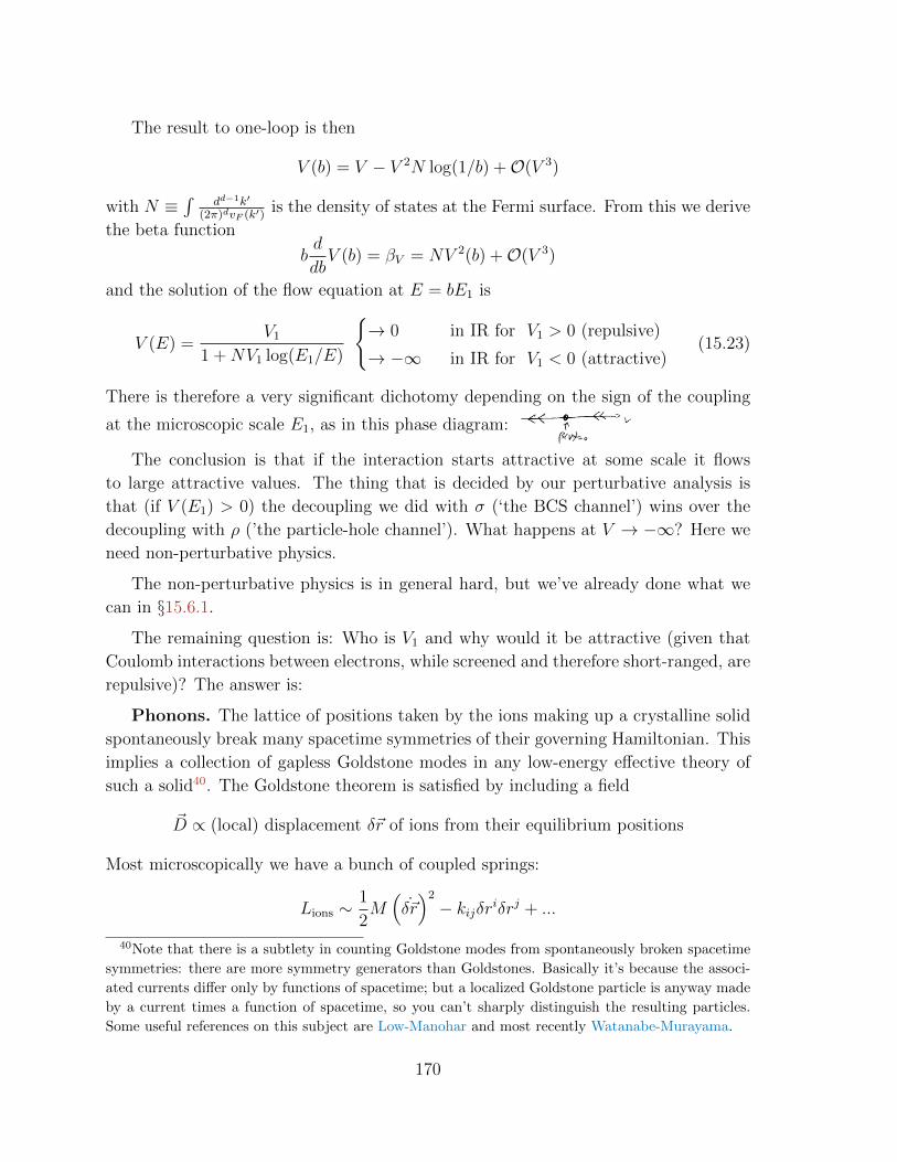
The result to one-loop is then
V (b) = V − V 2N log(1/b) +O(V 3)
with N ≡∫
dd−1k′
(2π)dvF (k′)is the density of states at the Fermi surface. From this we derive
the beta function
bd
dbV (b) = βV = NV 2(b) +O(V 3)
and the solution of the flow equation at E = bE1 is
V (E) =V1
1 +NV1 log(E1/E)
→ 0 in IR for V1 > 0 (repulsive)
→ −∞ in IR for V1 < 0 (attractive)(15.23)
There is therefore a very significant dichotomy depending on the sign of the coupling
at the microscopic scale E1, as in this phase diagram:
The conclusion is that if the interaction starts attractive at some scale it flows
to large attractive values. The thing that is decided by our perturbative analysis is
that (if V (E1) > 0) the decoupling we did with σ (‘the BCS channel’) wins over the
decoupling with ρ (’the particle-hole channel’). What happens at V → −∞? Here we
need non-perturbative physics.
The non-perturbative physics is in general hard, but we’ve already done what we
can in §15.6.1.
The remaining question is: Who is V1 and why would it be attractive (given that
Coulomb interactions between electrons, while screened and therefore short-ranged, are
repulsive)? The answer is:
Phonons. The lattice of positions taken by the ions making up a crystalline solid
spontaneously break many spacetime symmetries of their governing Hamiltonian. This
implies a collection of gapless Goldstone modes in any low-energy effective theory of
such a solid40. The Goldstone theorem is satisfied by including a field
~D ∝ (local) displacement δ~r of ions from their equilibrium positions
Most microscopically we have a bunch of coupled springs:
Lions ∼1
2M(
˙δ~r)2
− kijδriδrj + ...
40Note that there is a subtlety in counting Goldstone modes from spontaneously broken spacetime
symmetries: there are more symmetry generators than Goldstones. Basically it’s because the associ-
ated currents differ only by functions of spacetime; but a localized Goldstone particle is anyway made
by a current times a function of spacetime, so you can’t sharply distinguish the resulting particles.
Some useful references on this subject are Low-Manohar and most recently Watanabe-Murayama.
170
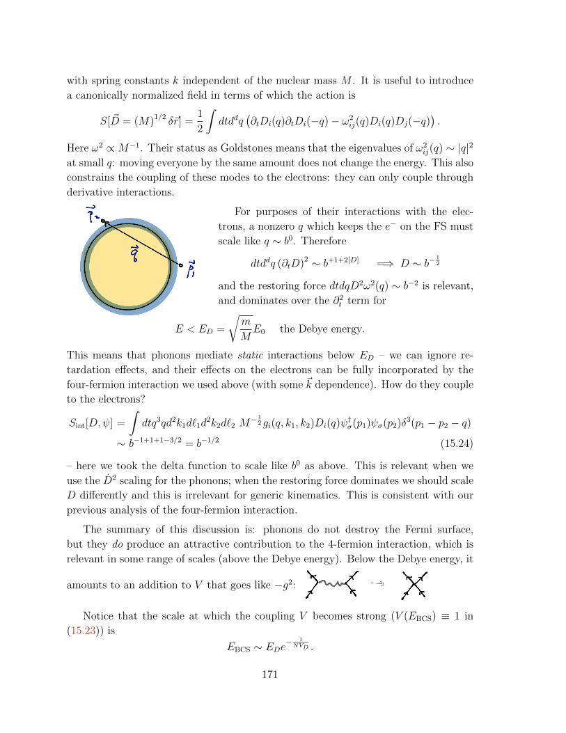
with spring constants k independent of the nuclear mass M . It is useful to introduce
a canonically normalized field in terms of which the action is
S[ ~D = (M)1/2 δ~r] =1
2
∫dtddq
(∂tDi(q)∂tDi(−q)− ω2
ij(q)Di(q)Dj(−q)).
Here ω2 ∝M−1. Their status as Goldstones means that the eigenvalues of ω2ij(q) ∼ |q|2
at small q: moving everyone by the same amount does not change the energy. This also
constrains the coupling of these modes to the electrons: they can only couple through
derivative interactions.
For purposes of their interactions with the elec-
trons, a nonzero q which keeps the e− on the FS must
scale like q ∼ b0. Therefore
dtddq (∂tD)2 ∼ b+1+2[D] =⇒ D ∼ b−12
and the restoring force dtdqD2ω2(q) ∼ b−2 is relevant,
and dominates over the ∂2t term for
E < ED =
√m
ME0 the Debye energy.
This means that phonons mediate static interactions below ED – we can ignore re-
tardation effects, and their effects on the electrons can be fully incorporated by the
four-fermion interaction we used above (with some ~k dependence). How do they couple
to the electrons?
Sint[D,ψ] =
∫dtq3qd2k1d`1d
2k2d`2 M− 1
2 gi(q, k1, k2)Di(q)ψ†σ(p1)ψσ(p2)δ3(p1 − p2 − q)
∼ b−1+1+1−3/2 = b−1/2 (15.24)
– here we took the delta function to scale like b0 as above. This is relevant when we
use the D2 scaling for the phonons; when the restoring force dominates we should scale
D differently and this is irrelevant for generic kinematics. This is consistent with our
previous analysis of the four-fermion interaction.
The summary of this discussion is: phonons do not destroy the Fermi surface,
but they do produce an attractive contribution to the 4-fermion interaction, which is
relevant in some range of scales (above the Debye energy). Below the Debye energy, it
amounts to an addition to V that goes like −g2:
Notice that the scale at which the coupling V becomes strong (V (EBCS) ≡ 1 in
(15.23)) is
EBCS ∼ EDe− 1NVD .
171
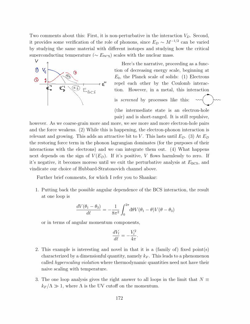
Two comments about this: First, it is non-perturbative in the interaction VD. Second,
it provides some verification of the role of phonons, since ED ∼ M−1/2 can be varied
by studying the same material with different isotopes and studying how the critical
superconducting temperature (∼ EBCS) scales with the nuclear mass.
Here’s the narrative, proceeding as a func-
tion of decreasing energy scale, beginning at
E0, the Planck scale of solids: (1) Electrons
repel each other by the Coulomb interac-
tion. However, in a metal, this interaction
is screened by processes like this:
(the intermediate state is an electron-hole
pair) and is short-ranged. It is still repulsive,
however. As we coarse-grain more and more, we see more and more electron-hole pairs
and the force weakens. (2) While this is happening, the electron-phonon interaction is
relevant and growing. This adds an attractive bit to V . This lasts until ED. (3) At EDthe restoring force term in the phonon lagrangian dominates (for the purposes of their
interactions with the electrons) and we can integrate them out. (4) What happens
next depends on the sign of V (ED). If it’s positive, V flows harmlessly to zero. If
it’s negative, it becomes moreso until we exit the perturbative analysis at EBCS, and
vindicate our choice of Hubbard-Stratonovich channel above.
Further brief comments, for which I refer you to Shankar:
1. Putting back the possible angular dependence of the BCS interaction, the result
at one loop is
dV (θ1 − θ3)
d`= − 1
8π2
∫ 2π
0
dθV (θ1 − θ)V (θ − θ3)
or in terms of angular momentum components,
dVld`
= −V2l
4π.
2. This example is interesting and novel in that it is a (family of) fixed point(s)
characterized by a dimensionful quantity, namely kF . This leads to a phenomenon
called hyperscaling violation where thermodynamic quantities need not have their
naive scaling with temperature.
3. The one loop analysis gives the right answer to all loops in the limit that N ≡kF/Λ 1, where Λ is the UV cutoff on the momentum.
172
4. The forward scattering interaction (for any choice of function F (θ13)) is not renor-
malized at one loop. This means it is exactly marginal at leading order in N .
5. Like in φ4 theory, the sunrise diagram at two loops is the first appearance of
wavefunction renormalization. In the context of the Fermi liquid theory, this
leads to the renormalization of the effective mass which is called m?.
Another consequence of the FS kinematics which I should emphasize more: it allows
the quasiparticle to be stable. The leading contribution to the decay rate of a one-
quasiparticle state with momentum k can be obtained applying the optical theorem to
the following process.
The intermediate state is two electrons with momenta k′ + q and k − q, and one
hole with momentum k′. The hole propagator has the opposite iη prescription. After
doing the frequency integrals by residues, we get
Σ(k, ε) =
∫dq dk′
|uq|2
D − iη
D ≡ εk(1 + iη) + εk′(1− iη)− εk′+q(1 + iη)− εk−q(1 + iη)
(Notice that this is the eyeball diagram which gives the lowest-order contribution to
the wavefunction renormalization of a field with quartic interactions.) By the optical
theorem, its imaginary part is the (leading contribution to the) inverse-lifetime of the
quasiparticle state with fixed k:
τ−1(k) = ImΣ(k, ε) = π
∫dq dk′δ(D)|uq|2f(−εk′)f(εk′+q)f(εk−q)
where
f(ε) = limT→0
1
eε−εFT + 1
= θ(ε < εF )
is the Fermi function. This is just the demand that a particle can only scatter into
an empty state and a hole can only scatter into a filled state. These constraints imply
that all the energies are near the Fermi energy: both εk′+q and εk′ lie in a shell of radius
ε about the FS; the answer is proportional to the density of possible final states, which
is thus
τ−1 ∝(ε
εF
)2
.
So the width of the quasiparticle resonance is
τ−1 ∝ ε2 ε
much smaller than its frequency – it is a sharp resonance, a well-defined particle.
173