IMM - DTU 02407 Stochastic Processes2017-10-30BFN/bfn

Lecture notes on phase–type distributions for 02407Stochastic Processes

Bo Friis Nielsen

October 2017

Contents

1 Phase–type distributions . . . . . . . . . . . . . . . . . . . . . . . . . . . . . . . . . . . . . . . . . . . . . . . . . . . . . . . . . . . . . . . 5

1.1 Notation . . . . . . . . . . . . . . . . . . . . . . . . . . . . . . . . . . . . . . . . . . . . . . . . . . . . . . . . . . . . . . . . . . . . . . . . . 5

1.2 Matrix results . . . . . . . . . . . . . . . . . . . . . . . . . . . . . . . . . . . . . . . . . . . . . . . . . . . . . . . . . . . . . . . . . . . . . 5

1.2.1 The Kronecker product . . . . . . . . . . . . . . . . . . . . . . . . . . . . . . . . . . . . . . . . . . . . . . . . . . . . . . 6

1.3 Discrete phase–type distributions . . . . . . . . . . . . . . . . . . . . . . . . . . . . . . . . . . . . . . . . . . . . . . . . . . . . 7

1.3.1 Cumulative distribution and probability mass function . . . . . . . . . . . . . . . . . . . . . . . . . . . . 8

1.3.2 The generating function . . . . . . . . . . . . . . . . . . . . . . . . . . . . . . . . . . . . . . . . . . . . . . . . . . . . . . 8

1.3.3 Moments . . . . . . . . . . . . . . . . . . . . . . . . . . . . . . . . . . . . . . . . . . . . . . . . . . . . . . . . . . . . . . . . . . 9

1.3.4 Closure properties . . . . . . . . . . . . . . . . . . . . . . . . . . . . . . . . . . . . . . . . . . . . . . . . . . . . . . . . . . 9

1.3.5 Non–uniqueness of representations . . . . . . . . . . . . . . . . . . . . . . . . . . . . . . . . . . . . . . . . . . . . 12

1.4 Continuous phase–type distributions . . . . . . . . . . . . . . . . . . . . . . . . . . . . . . . . . . . . . . . . . . . . . . . . . . 13

1.4.1 Probability functions . . . . . . . . . . . . . . . . . . . . . . . . . . . . . . . . . . . . . . . . . . . . . . . . . . . . . . . . 13

1.4.2 The Laplace-transform . . . . . . . . . . . . . . . . . . . . . . . . . . . . . . . . . . . . . . . . . . . . . . . . . . . . . . . 14

1.4.3 Moments . . . . . . . . . . . . . . . . . . . . . . . . . . . . . . . . . . . . . . . . . . . . . . . . . . . . . . . . . . . . . . . . . . 14

1.4.4 Evaluation of continuous phase–type distributions . . . . . . . . . . . . . . . . . . . . . . . . . . . . . . . . 15

1.4.5 Properties of continuous phase–type distributions . . . . . . . . . . . . . . . . . . . . . . . . . . . . . . . . 15

1.4.6 Phase–type renewal process . . . . . . . . . . . . . . . . . . . . . . . . . . . . . . . . . . . . . . . . . . . . . . . . . . 18

1.4.7 Non–uniqueness of continuous phase–type distributions . . . . . . . . . . . . . . . . . . . . . . . . . . . 19

3

4

References . . . . . . . . . . . . . . . . . . . . . . . . . . . . . . . . . . . . . . . . . . . . . . . . . . . . . . . . . . . . . . . . . . . . . . . . . . . . . . . . 21

Chapter 1

Phase–type distributions

1.1 Notation

We will use 1 to denote a column vector of ones of appropriate dimension.

1 =

11...1

.

Correspondingly we will let 000 denote the vector of zeros.

Matrices is represented by capital primarily roman letters like TTT and AAA. The symbol III will be used for a unitymatrix of appropriate dimension while, while 000 is a matrix of zero’s of appropriate dimension.

1.2 Matrix results

In this section we have collected a few slightly specialized matrix results.

Lemma 1. The inverse of the block Matrix �AAA BBB000 CCC

�(1.1)

is �AAA−1 −AAA−1BBBCCC−1

000 CCC−1

�(1.2)

whenever AAA and CCC are invertible.

Proof. By direct verification.

5

6

1.2.1 The Kronecker product

Many operations with phase–distributions are conveniently expressed using the Kronecker product. For twomatrices AAA with dimension �× k and BBB with dimension n×m we define the Kroneckerproduct ⊗ by

AAA⊗BBB =

a11BBB a12BBB . . . a1kBBBa21BBB a22BBB . . . a2kBBB

... . . ....

...a�1BBB a�2BBB . . . a�kBBB

(1.3)

Example 1. Consider the matrices AAA, BBB, and III given by:

AAA =

�2 7 13 5 11

�, BBB =

�13 40 17

�, III =

1 0 00 1 00 0 1

.

Then AAA⊗BBB, AAA⊗ III and III ⊗BBB is given by

AAA⊗BBB =

2 ·13 2 ·4 7 ·13 7 ·4 1 ·13 1 ·42 ·0 2 ·17 7 ·0 7 ·17 1 ·0 1 ·17

3 ·13 3 ·4 5 ·13 5 ·4 11 ·13 11 ·43 ·0 3 ·17 5 ·0 5 ·17 11 ·0 11 ·17

AAA⊗ III =

2 0 0 7 0 0 1 0 00 2 0 0 7 0 0 1 00 0 2 0 0 7 0 0 13 0 0 5 0 0 11 0 00 3 0 0 5 0 0 11 00 0 3 0 0 5 0 0 11

III ⊗BBB =

13 4 0 0 0 00 17 0 0 0 00 0 13 4 0 00 0 0 17 0 00 0 0 0 13 40 0 0 0 0 17

.

The following rule is very convenient. If the usual matrix products LLLUUU and MMMVVV exist, then

(LLL⊗MMM)(U⊗V) = LLLUUU ⊗MMMVVV . (1.4)

A natural operation for continuous time phase–type distributions is AAA⊗ III+ III⊗BBB, thus motivating the definitionof the Kronecker sum defined by the symbol ⊕.

AAA⊕BBB = AAA⊗ III + III ⊗BBB (1.5)

7

1.3 Discrete phase–type distributions

Definition 1. A discrete phase–type distribution is the distribution of the time to absorption in a finite discretetime Markov chain with transition matrix PPP of dimension m+ 1 is given by 1.6. The Markov chain has mtransient and 1 absorbing state.

PPP =

�TTT ttt000 1

�. (1.6)

The initial probability vector is denoted by (ααα,αm+1). The pair (ααα,TTT ) is called a representation for the phase–type distribution.

The matrix (III−TTT ) is non–singular (i.e. the only solution to xxx = xxxTTT is xxx = 000). One consequence is, that at leastone of the row sums of TTT is strictly less than 1. As PPP is a stochastic matrix it satisfies equation 1.7.

PPP1 = 1 (1.7)

and we haveTTT 1+ttt = 1 or ttt = (III −TTT )1 . (1.8)

It follows from

PPPn =

�TTT n (III −TTT n)1000 1

�

thatP(X > n) =αααTTT n1 .

ThusP(X ≤ n) = 1−αααTTT n1 . (1.9)

Example 2. The simplest possible discrete phase–type distribution is obtained, when the dimension of TTT ism=1. In this case we have

PPP =

�p 1− p0 1

�

ααα = (1). As will be clear later this phase–type distribution is simply a geometric distribution with parameter1− p. A sum of geometrically distributed random variables has a negative binomial distribution. The negativebinomial distribution can be expressed as a phase–type distribution by

PPP =

p 1− p 0 0 . . . 0 0 00 p 1− p 0 . . . 0 0 00 0 p 1− p . . . 0 0 0...

......

......

......

0 0 0 0 . . . p 1− p 00 0 0 0 . . . 0 p 1− p

000 1

ααα = (1,0, . . . ,0).

8

1.3.1 Cumulative distribution and probability mass function

We will now give the argument leading to formula (1.9) in more detail. We first consider the probabilities forthe transient states after n transitions. That is p(n)i = Prob(Xn = i). We collect these probabilities in a vector toget ppp(n) = (p(n)1 , . . . , p(n)m ). Using standard arguments for discrete time Markov chains we get

ppp(n) = ppp(n−1)TTT =αααTTT n . (1.10)

The event that absorption occurs at time x can be partitioned using the union of the events that the chain is instate i (i = 1, . . . ,m) at time x− 1, and that absorption happens at i at time x. The probability of the former isp(x−1)

i while the probability of the latter event is ti. Thus the probability mass function can be expressed as

f (x) =m

∑i=1

p(x−1)i ti = ppp(x−1)ttt =αααTTT x−1ttt, x > 0 . (1.11)

The cumulative probability function can now be find by summation of f (x) or by noting the absorption hasoccurred if the process is no longer in one of the transient states at time x. The probability of being in one ofthe transient states is ∑m

i=1 p(x)i = ppp(x)1 =αααTTT x1. Thus, the cumulative distribution function is given by

F(x) = 1−αααTTT x1, x ≥ 0 (1.12)

Example 3. For the geometric distribution in Example 2 we find using (1.11) and (1.12):

f (x) = 1 · px−1(1− p) (1.13)

F(x) = 1−1 · px (1.14)

(1.15)

1.3.2 The generating function

The generating function for a non–negative discrete random variable X is given by (1.16)

H(z) = E�zX�=

∞

∑x=0

zx f (x) (1.16)

For a discrete phase–type random variable we find

H(z) =∞

∑x=0

zx f (x) = αm+1 +∞

∑x=1

zxαααTTT x−1ttt = αm+1 + zααα(III − zTTT )−1ttt (1.17)

Here we have used the geometric series ∑∞i=0 xi = 1

1−x for matrices. (see e.g. [2] Theorem 28.1). The result is∑∞

i=0 AAAi = (III −AAA)−1 whenever |λi|< 1 for all i, where λi are the eigenvalues of AAA.

Example 4. For the geometric distribution we get the well–known result

9

H(z) = z(1− pz)−1(1− p) =z(1− p)1− zp

(1.18)

1.3.3 Moments

The factorial moments for a discrete random variable can be obtained by successive differentiation of thegenerating function.

E(X(X −1) . . .(X − (k−1)) =dH(z)k

dzk

�����z=1

.

Thus for a discrete phase–type variable with representation (ααα,TTT ) we get

E(X(X −1) . . .(X − (k−1))) = k!ααα(III −TTT )−kTTT k−11 .

The matrix UUU = (III −TTT )−1 is of special importance as the i, j’th element has an important probabilistic inter-pretation as the expected time spent in state j before absorption conditioned on starting in state i. By a little bitof matrix calculation we can express the generating function using UUU rather than TTT to get

H(z) = αm+1 +ααα�

UUU1− z

z+ III

�−1

1 ,

(where the latter expression obviously is not defined for z = 0).

1.3.4 Closure properties

One of the appealing features of phase–type distributions is that the class is closed under a number of oper-ations. The closure properties are a main contributing factor to the popularity of phase–type distributions inprobabilistic modeling of technical systems. In particular we will see the that the class is closed under addition,finite mixtures, and finite order statistics.

Theorem 1. [Sum of two independent PH variables] Consider to discrete random variables X and Y withrepresentation (ααα,TTT ) and (βββ ,SSS) respectively. Then the random variable Z = X +Y follows a discrete phase–type distribution with representation (γγγ,L) given by 1.19.

�LLL lll000 1

�=

T11 T12 . . . T1m t1β1 t1β2 . . . t1βk t1βk+1T21 T22 . . . T2m t2β1 t2β2 . . . t2βk t2βk+1

......

......

......

......

...Tm1 Tm2 . . . Tmm tmβ1 tmβ2 . . . tmβk tmβk+10 0 . . . 0 S11 S12 . . . S1k s10 0 . . . 0 S21 S22 . . . S2k s2...

......

......

......

......

0 0 . . . 0 Sk1 Sk2 . . . Skk sk0 0 . . . 0 0 0 . . . 0 1

, (1.19)

γγγ = (α1,α2, . . . ,αm,αm+1β1,αm+1β2, . . . ,αm+1βk). In matrix notation

10

�LLL lll000 1

�=

TTT tttβββ βk+1ttt0 SSS sss

000 1

(1.20)

γγγ = (ααα,αm+1βββ ),γm+k+1 = αm+1βk+1.

Proof. The probabilistic proof is straightforward by concatenating the transition matrices for the transient statesof the Markov chains related to X and Y . We interpret the random variables Z, X , and Y as time variables. Inorder to get the random variable Z we first start a Markov chain related to X given by (ααα,TTT ). Immediately uponabsorption from X we start the Markov chain related to Y given by (βββ ,SSS). The terms tiβ j ensures that the initialprobability distribution of the Y chain is indeed βββ .

One can alternatively proceed entirely analytically by manipulations with generating functions.

Hz(z) = Hx(z)Hy(z) = (αm+1 + zααα(III − zTTT )−1ttt)(βk+1 + zβββ (III − zSSS)−1sss) (1.21)

After some straightforward but tedious calculations, we omit the details for now, one obtains

Hz(z) = γm+1 + zγγγ(III − zL)−1lll (1.22)

Remark 1. An important implication is that the representation for a phase–type distribution can not be uniqueas the representation for Z = X +Y is not in general symmetric in the parameters of the X and Y chains.Thus, typically the L matrix will be different depending on which chain we choose to represent X while theexpressions for the distribution like F(x), f (x) or H(z) will be identical. See Section 1.3.5 for a somewhatdeeper discussion of this and some supplementary examples.

1.3.4.1 Finite mixtures of phase–type distributions

Given Xi phase–type distributed with representation (αiαiαi,TTT i) we have Z = IiXi with ∑ki=1 Ii = 1 and P(Ii = 1) =

pi). It is easy to see that the random variable Z is itself phase–type distributed with representation (γγγ,L) givenby 1.23:

L =

TTT 1 0 . . . 00 TTT 2 . . . 0...

......

...0 0 . . . TTT k

(1.23)

γγγ = (p1α1α1α1, p2α2α2α2, . . . , pkαkαkαk).

Example 5. For two geometric distributions with parameters px and py we have the representation

L =

�px 00 py

�

with γγγ = (p0x, p0y) = (p0x,1− p0x), where p0x is the probability of choosing the first respectively the secondgeometric distribution.

11

1.3.4.2 Order statistics

Initially we focus on the distribution of the smallest U and the largest V of two independent variables X and Y .Thus U = min(X ,Y ) and V = max(X ,Y ). First we will consider the following basic example.

Example 6. Let X be negative binomially distributed with parameters kx = 2, px and let Y be negative binomiallydistributed with parameters ky = 2, py. The matrix TTT x is given by

TTT x =

�px 1− px0 px

�TTT y =

�py 1− py0 py

�

with αxαxαx = (1,0) and αyαyαy = (1,0). We define Z = min(X ,Y ) and proceed by creating a Markov chain thatdescribes the simultaneous evolution of the X and the Y chains and thus the evolution of the Z chain. Theprocess will have 4 transient states corresponding to all possible combinations of the X and Y chains. Wedenote the four states by (1,1),(1,2),(2,1),(2,2). The transition from (1,1) to (1,2) occurs whenever we haveno state change in the X chain (probability px) and the Y chain changes state (probability 1− py). In summarythe final Markov chain tracks the time until the first of the two original chains reaches the absorbing state. Thus,

TTT min(X ,Y ) =

px py px(1− py) (1− px)py (1− px)(1− py)0 px py 0 (1− px)py0 0 px py px(1− py)0 0 0 px py

and we have that αmin(X ,Y )αmin(X ,Y )αmin(X ,Y ) = (1,0,0,0). Further, we see that we can write TTT min(X ,Y ) = TTT x ⊗TTT y and αmin(X ,Y )αmin(X ,Y )αmin(X ,Y ) =αxαxαx ⊗αyαyαy.With respect to the distribution of Z2 = max(X ,Y ) we need to include 4 more states (1,3),(2,3),(3,1),(3,2)corresponding to the possibility that one of the two chains survives the absorption of the other. It is convenientto order the state space as (1,1),(1,2),(2,1),(2,2),(1,3),(2,3),(3,1),(3,2). And we obtain the phase typegenerator TTT max(X ,Y )

TTT max(X ,Y ) =

px py px(1− py) (1− px)py (1− px)(1− py) 0 0 0 00 px py 0 (1− px)py px(1− py) (1− px)(1− py) 0 00 0 px py px(1− py) 0 0 (1− px)py (1− px)(1− py)0 0 0 px py 0 px(1− py) 0 (1− px)py)0 0 0 0 px 1− px 0 00 0 0 0 0 px 0 00 0 0 0 0 0 py 1− py0 0 0 0 0 0 0 py

The general result is that for X phase–type distributed with (TTT x,αxαxαx) and Y phase–type distributed with (TTT y,αyαyαy)is min(X ,Y ) phase–type distributed with representation (L,γγγ) given by 1.24:

L = TTT x ⊗TTT y , (1.24)

where γγγ =αxαxαx ⊗αyαyαy. Further max(X ,Y ) is phase–type distributed with representation (L,γγγ) given by 1.25:

L =

TTT x ⊗TTT y TTT x ⊗ttty tttx ⊗TTT y0 TTT x 00 0 TTT y

(1.25)

med γγγ = (αxαxαx ⊗αyαyαy,αxαxαxαy,m+1,αx,k+1αyαyαy). Here the dimension of TTT x is k and the dimension of TTT y is m. We writelll explicitly:

12

lll =

tttx ⊗tttytttxttty

(1.26)

1.3.4.3 Other properties

We briefly mention that all discrete probability distribution functions with finite support (i.e. f (x) = 0 for allx ≥ x0) are of phase–type.

Random sum of independent discrete phase–type variables where the number of terms in the random sum isitself phase–type distributed is phase type distributed with representation.

(ααα ⊗βββ ,TTT ⊗ III +tttααα ⊗SSS)

1.3.5 Non–uniqueness of representations

A main drawback when modeling with phase–type distributions is the non–uniqueness of their representations.Thus in most cases a number of different representations will give rise to the same distribution. Thus, only invery special cases will a representation be unique.

Example 7. The distribution with representation ((1,0),TTT ) with TTT given by

TTT =

�p1 p2 − p10 p2

�(1.27)

is simply a geometric distribution with f (x) = px−12 (1− p2).

. This can be seen by deriving the generating function for the distribution. Alternatively it is seen that ttt =�1− p21− p2

�, thus there is a constant probability 1− p2 of absorption not dependent on the state of the chain and

thus independent of.

13

1.4 Continuous phase–type distributions

Many definitions and results regarding discrete time phase–type distributions carry over verbatim to the con-tinuous time case, other need minor modifications. We first extend Definition 1 in.

Definition 2. A phase–type distribution is the distribution of the time to absorption in a finite Markov chain ofdimension m+1, where one state is absorbing and the remaining m states are transient. A phase type distributionis uniquely given by an m dimensional row vector ααα and an m×m matrix TTT . We call the the pair (ααα,TTT )arepresentation for the phase type distribution. The vector ααα can be interpreted as the initial probability vectoramong the m transient states, while the the matrix TTT can be interpreted as the one step transition probabilitymatrix among the transient states in the discrete case and as the infinitesimal generator matrix among thetransient states in the continuous case. A phase–type distribution is uniquely given by any representation.However, several representations can lead to the same phase–type distribution. We will elaborate a little bit onthis in Section 1.4.7.

The generator matrix for the Markov chain in the continuous case for a given representation is given by (1.28)

Q =

�TTT ttt000 0

�(1.28)

This section will be quite repetitive restating a number of results now for the continuous case. In some case theexact formulation of results and properties will vary slightly.

1.4.1 Probability functions

Once again the most apparent result regards the survival function.

As in Section 1.3.1 we will consider the probabilities pi(t)(i = 1, . . . ,m) of the Markov chain being intransient state i at time t. We collect these probabilities in the vector ppp(t). Further we define the vectorp+p+p+(t) = (ppp(t), pm+1(t)), which can be found as the standard solution to the Chapman-Kolmogorov equations

p+p+p+�(t) = p+p+p+(t)Q , (1.29)

such that ppp(t) satisfies:ppp�(t) = ppp(t)TTT . (1.30)

The solution to this system is ppp(t) =αααetTTT ([1] page 182). Thus the probability that the chain is not yet absorbedat time t is ppp(t)1 =αααetTTT = P(X > t). We get

P{X ≤ x}= F(x) = 1−αααeTTT x1 . (1.31)

Now using exTTT = ∑∞i=0

(xTTT )i

i! we find f (x) = F �(x) =−αααeTTT xTTT 1. Finally using TTT 1+ttt = 000 we get

f (x) =αααeTTT xttt . (1.32)

Example 8. Choosing the dimension of TTT to be 1 we find the

14

Q =

�−λ λ0 0

�

corresponding to the phase–type representation ((1), [−λ ]). We find F(t) = 1− e−λ t and f (t) = λe−λ t - anexponential distribution.

1.4.2 The Laplace-transform

The Laplace transform of a continuous probability distribution for the random variable X is defined by E(e−sX .For the continuous part of a phase type distribution we need to evaluate

� ∞0 e−st f (t)dt =ααα(sIII−TTT )−1ttt, and we

getE(e−sX = H(s) = αm+1 +ααα(sIII −TTT )−1ttt (1.33)

Theorem 2. Let UUU = (−TTT )−1, then the (i, j)th element ui j is the expected time spent in state j given initiationin state i prior to absorption.

Proof. Let Z j denote the time spent in state j prior to absorption. Then

Ei(Z j) = Ei

�� τ

0δX(t)= jdt

�

=� ∞

0Ei

�δX(t)= jδτ≥t

�dt

=� ∞

0¶i�δX(t)= jδτ≥t

�dt

=� ∞

0

�eTTTt

�i j

dt

= (−TTT )−1

1.4.3 Moments

We now have

Corollary 1. The mean of a PH(ααα,TTT ) distributed random variable is αααUUU1.

Proof. Just notice that UUU1 is the vector which i’th element is the expected time the process spends in any stateprior to absorption given initiation in state i.

We can alternatively get mean and the all non–central moments by successive differentiation of the Laplacetransform. Doing this yields

µi = i!ααα(−TTT )−i1 (1.34)

15

1.4.4 Evaluation of continuous phase–type distributions

Phase–type distributions have a rational Laplace transform. The cumulative distribution function and the prob-ability density function will thus consist of terms of the form

ticos(ωt)e−λ t ,

where i or ω could be 0 leading to simpler expressions.

In order to get such explicit (scalar) expressions one can use the following approach.

• Calculate eTTTt by deriving the first terms in the series ∑∞i=0

(TTTt)i

i! and then prove a general result by induction.However, this approach is usually quite cumbersome and difficult. Generally the TTT matrix should be upperor lower diagonal for this approach to be viable.

• Alternatively one can determine the Laplace transform, find the roots of the denominator, and then use apartial fraction expansion. Inversion of each term in the fractional expansion is now straightforward. How-ever, to find the roots of the denominator is equivalent to finding the root of an m’th order polynomial whichis non–trivial in general.

The numerical evaluation is straightforward if one of the two above mentioned methods works. In general onemust resort to numerical solution of the linear equation system governing the probabilities ppp(t), i.e. solvingthe Chapman Kolmogorov equations numerically. There is a very efficient method called uniformization forcalculating this solution. Introducing the quantity θ =−min(Tii) one rewrites TTT = θ(KKK − III). The matrix KKK isa sub-stochastic matrix such that KKK = III +θ−1TTT . Now

αααeTTTt1 = e−θ t∞

∑i=0

αααθ iKKKi1i!

ti .

This formula is very well suited for numerical evaluation as all terms in the series are non–negative and sincean appropriate level for truncation of the sum can be derived from the Poisson distribution.

1.4.5 Properties of continuous phase–type distributions

As for discrete phase–type distribution the class of phase–type distributions is closed under a number of stan-dard operations occurring frequently in probability theory.

1.4.5.1 Addition of two random variables

Theorem 3. For X ∈PH(ααα,TTT ) and Y ∈PH(βββ ,SSS) and independent Z =X +Y ∈PH(γγγ,LLL) with γγγ = (ααα,αm+1βββ )and �

LLL lll000 0

�=

TTT tttβββ βk+1ttt0 SSS sss

000 0

(1.35)

16

�LLL lll000 0

�=

T11 T12 . . . T1m t1β1 t1β2 . . . t1βk t1βk+1T21 T22 . . . T2m t2β1 t2β2 . . . t2βk t2βk+1

......

......

......

......

...Tm1 Tm2 . . . Tmm tmβ1 tmβ2 . . . tmβk tmβk+10 0 . . . 0 S11 S12 . . . S1k s10 0 . . . 0 S21 S22 . . . S2k s2...

......

......

......

......

0 0 . . . 0 Sk1 Sk2 . . . Skk sk0 0 . . . 0 0 0 . . . 0 0

(1.36)

γγγ = (α1,α2, . . . ,αm,αm+1β1,αm+1β2, . . . ,αm+1βk). In matrix notation γγγ = (ααα,αm+1βββ ).

Example 9. Consider the sum Z = ∑ki=1 Xi with Xi ∈ exp(λi). Using 1.35 we get

TTT =

−λ1 λ1 0 0 . . . 0 0 00 −λ2 λ2 0 . . . 0 0 00 0 −λ3 λ3 . . . 0 0 00 0 0 −λ4 . . . 0 0 0...

......

......

......

...0 0 0 0 . . . −λk−2 λk−2 00 0 0 0 . . . 0 −λk−1 λk−10 0 0 0 . . . 0 0 −λk

ααα = (1,0, . . . ,0). With λi = λ we get a sum of identically distributed exponential random variables, referredto as an Erlang–distribution. These distributions are special cases of the gamma distribution with integer shapeparameter. We have

f (x) = λ (λx)k−1

(k−1)! e−λx (1.37)

F(x) = ∑∞i=k

(λx)i

i! e−λx = 1−k−1

∑i=0

(λx)i

i!e−λx (1.38)

H(s) =�

λs+λ

�k(1.39)

µi =(i+k−1)!(k−1)!λ i (1.40)

1.4.5.2 Finite mixtures

We restate a result which is identical to the discrete case even in formulation

Theorem 4. Any finite convex mixture of phase–type distribution is a phase type distribution. Let Xi ∈PH(ααα i,TTT i) i= 1, . . . ,k such that Z =Xi with probability pi Then Z ∈PH(γγγ,LLL) where γγγ =(p1α1α1α1, p2α2α2α2, . . . , pkαkαkαk)and

17

LLL =

TTT 1 0 . . . 00 TTT 2 . . . 0...

......

...0 0 . . . TTT k

(1.41)

Proof. Directly using the probabilistic interpretation of (γγγ,LLL).

Example 10. Consider the k random variables Xi ∈ exp(λi) and assume that Z takes the value of Xi with prob-ability pi. The distribution of Z can be expressed as a proper mixture of the Xi’s. fz(x) = ∑k

i=1 piλie−λix. Thedistribution of Z is called a hyper exponential distribution. using 1.41 we find a phase–type representation (γγγ,LLL)for Z. γγγ = (p1, p2, . . . , pk).

LLL =

−λ1 0 . . . 00 −λ2 . . . 0...

......

...0 0 . . . −λk

(1.42)

The hyper-exponential distribution is quite important and we mention its characteristics explicitly.

f (x) = ∑ki=1 piλie−λix (1.43)

F(x) = 1−∑ki=1 pie−λix (1.44)

H(s) = ∑ki=1

piλis+λi

(1.45)

µi = i!∑ki=1

piλ i

i(1.46)

1.4.5.3 Order statistics

The order statistic of a finite number of independent discrete phase–type distributed variables is itself phase–type distributed. We will focus on the distribution of the smallest and the largest of two independent variablesX with representation (αααx,TTT x) and Y with representation (αααy,TTT y). We motivate the derivation with a smallexample.

Example 11. Let X be generalized Erlang distributed with parameters λx,1,λx,2 and let Y be hyper-exponentiallydistributed with parameters py,λy,1,λy,2. We will first investigate the distribution of min(X ,Y ). We have

TTT x =

�−λx,1 λx,1

0 −λx,2

�TTT y =

�−λy,1 0

0 −λy,2

�

with αxαxαx = (1,0) and αyαyαy = (py,1− py). We can now construct a Markov chain that simultaneously describesthe evolution of the two chains related to X and Y respectively. As for Example 6 the chain will have 4 statescorresponding to the all possible combinations of the states of the two original chains.

We denote the four states by (1,1),(1,2),(2,1),(2,2). The transitions from (1,1) to (2,1), and from (1,2) to(2,2) occur with intensity λx,1, while no other transitions are possible from these two states. The remainingtransitions are found similarly. In summary we get a Markov chain that describes the time until the first of thetwo chain get absorbed (min(X ,Y )). This time is obviously then phase–type distributed with generator

18

TTT min(X ,Y ) =

−(λx,1 +λy,1) 0 λx,1 00 −(λx,1 +λy,2) 0 λx,10 0 −(λx,2 +λy,1) 00 0 0 −(λx,2 +λy,2)

and with initial probability vector αmin(X ,Y )αmin(X ,Y )αmin(X ,Y ) = (py,1− py,0,0). Further we have TTT min(X ,Y ) = TTT x ⊗ III + III ⊗TTT yand αmin(X ,Y )αmin(X ,Y )αmin(X ,Y ) =αxαxαx ⊗αyαyαy.

To get the distribution of max(X ,Y ) we need additionally to consider the states (1,3),(2,3),(3,1),(3,2) corre-sponding to the event that one of the chains has reached the absorbing state. It is convenient to use the ordering(1,1),(1,2),(2,1),(2,2),(1,3),(2,3),(3,1),(3,2). And we find TTT max(X ,Y ) to be

TTT max(X ,Y ) =

−(λx,1 +λy,1) 0 λx,1 0 λy,1 0 0 00 −(λx,1 +λy,2) 0 λx,1 λy,2 0 0 00 0 −(λx,2 +λy,1) 0 0 λy,1 λx,2 00 0 0 −(λx,2 +λy,2) 0 λy,2 0 λx,20 0 0 0 −λx,1 λx,1 0 00 0 0 0 0 −λx,2 0 00 0 0 0 0 0 −λy,1 00 0 0 0 0 0 0 −λy,2

Theorem 5. For X ∈ PH(TTT x,αxαxαx) and Y ∈ PH(TTT y,αyαyαy) is min(X ,Y ) phase distributed with representation (LLL,γγγ)given by 1.47:

LLL = TTT x ⊗ IIIy + IIIx ⊗TTT y , (1.47)

where γγγ =αxαxαx ⊗αyαyαy. and max(X ,Y ) is phase type distributed with representation (LLL,γγγ) given by 1.48:

LLL =

TTT x ⊗ IIIy + IIIx ⊗TTT y IIIx ⊗ttty tttx ⊗ IIIy0 TTT x 00 0 TTT y

(1.48)

med γγγ = (αxαxαx ⊗αyαyαy,αxαxαxαy,m+1,αx,k+1αyαyαy). where the dimension of TTT x is k and the dimension of TTT y is m. We give lllexplicitly

lll =

000tttxttty

(1.49)

1.4.6 Phase–type renewal process

A phase–type renewal process is a point process, were the distance between two points can be described byindependent and identically distributed phase–type distributed random variables. The stationary version is ofspecial interest. The age of the process at time t is defined to be the time since the last event - or point - whilethe residual life time at time t is the time to the next event - or point. We have the following important result.

Theorem 6. In a stationary phase–type renewal process the distribution of age and residual life time are phase–type distributed with representation (πππ,TTT ) where πππ = αααUUU

αααUUU1 .

19

Proof. The phase process J(t) is a finite continuous time Markov chain with generator matrix QQQ = TTT + tttαααof dimension m. The stationary probability vector πππ for this chain satisfies πππ(TTT + tttααα) = 000 or equivalentlyπππ = πππtttαααUUU . By probabilistic reasoning or by post-multiplying with 1 we see that πππttt = 1

αααUUU1 . At an arbitraryepoch the probabilistic distribution among the states in the Markov chain is given by πππ . From this point thetime to absorption will be phase type distributed with the representation of the theorem. The distribution of agemust be the same by symmetry.

Corollary 2. The moments of the residual life time distribution is given by. Der gælder følgende formel formomenterne af restlevetidsfordelingen:

µ�i = i!

αααUUU−i+11αααUUU1

. (1.50)

Proof. The corollary follows directly from Theorem 6 and the equation for the moments of a phase–typedistribution as given in Section 1.4.3.

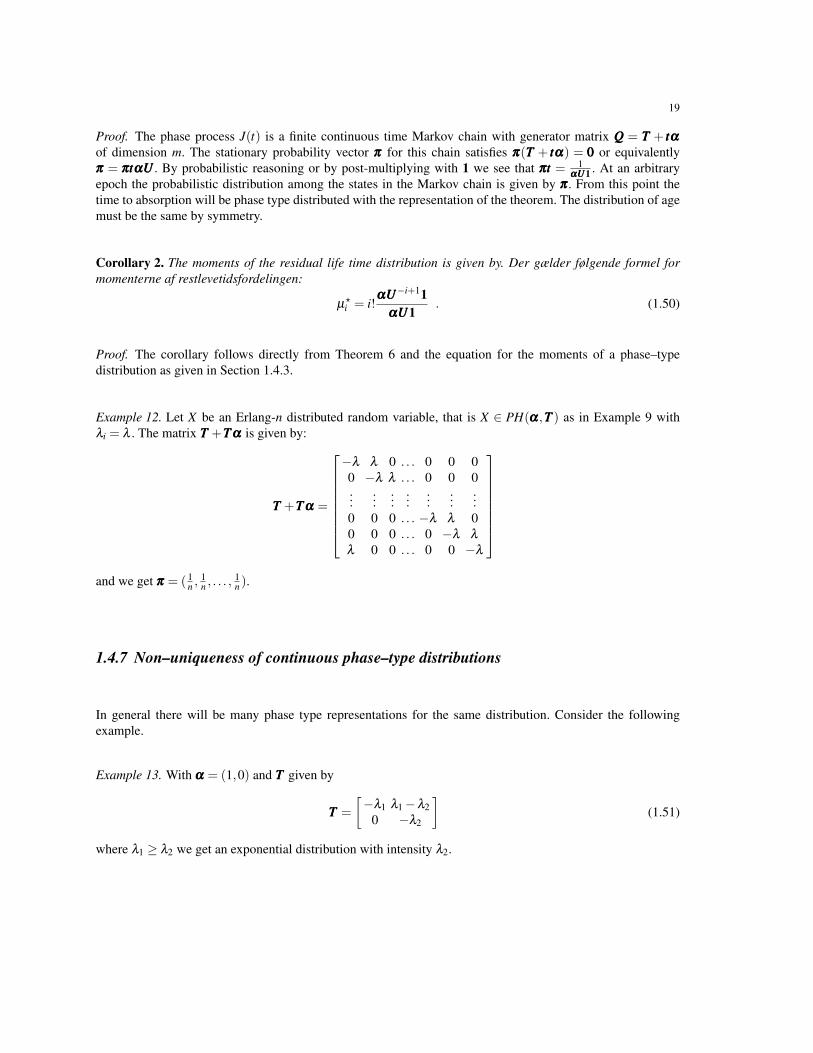
Example 12. Let X be an Erlang-n distributed random variable, that is X ∈ PH(ααα,TTT ) as in Example 9 withλi = λ . The matrix TTT +TTTααα is given by:

TTT +TTTααα =

−λ λ 0 . . . 0 0 00 −λ λ . . . 0 0 0...

......

......

......

0 0 0 . . . −λ λ 00 0 0 . . . 0 −λ λλ 0 0 . . . 0 0 −λ

and we get πππ = ( 1n ,

1n , . . . ,

1n ).

1.4.7 Non–uniqueness of continuous phase–type distributions

In general there will be many phase type representations for the same distribution. Consider the followingexample.

Example 13. With ααα = (1,0) and TTT given by

TTT =

�−λ1 λ1 −λ2

0 −λ2

�(1.51)

where λ1 ≥ λ2 we get an exponential distribution with intensity λ2.

References

1. D. R. Cox and H. D. Miller. The Theory of Stochastic Processes. Chapman and Hall, 1980.2. Ole Groth Jørsboe. Funktionalanalyse. Matematisk Institut. Danmarks Tekniske Højskole, 1987.

21